routing in data networks - mit
TRANSCRIPT
MIT
Routing in Data Networks
Muriel MedardEECSLIDS
MIT
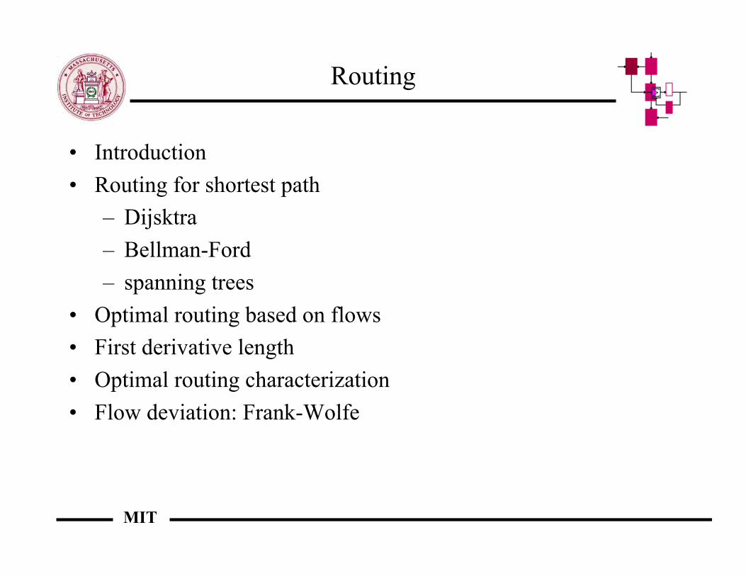
Routing
• Introduction• Routing for shortest path
– Dijsktra– Bellman-Ford– spanning trees
• Optimal routing based on flows• First derivative length• Optimal routing characterization• Flow deviation: Frank-Wolfe
MIT
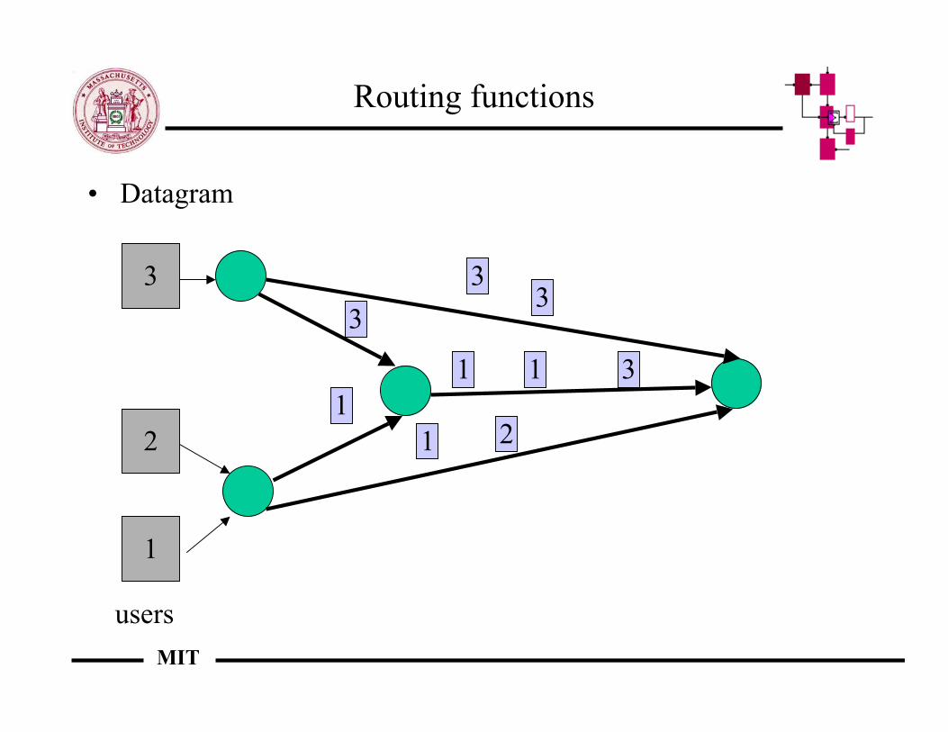
Routing functions
• Datagram
3
2
1
users
11
1
1
2
33
3
3
MIT
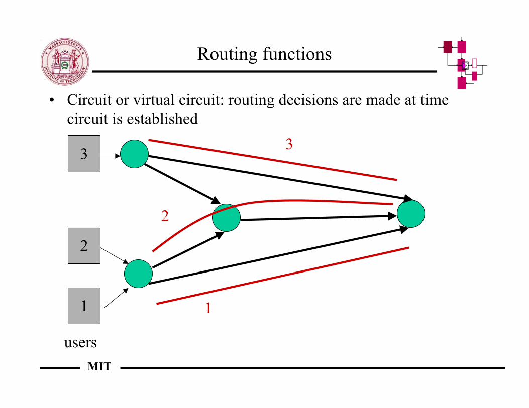
Routing functions
3
2
1
users
• Circuit or virtual circuit: routing decisions are made at timecircuit is established
1
3
2
MIT
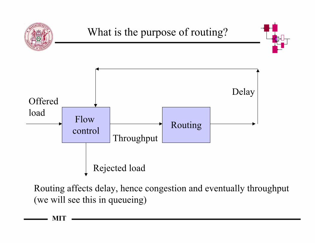
What is the purpose of routing?
Flow control Routing
Offeredload
Throughput
Rejected load
Delay
Routing affects delay, hence congestion and eventually throughput(we will see this in queueing)
MIT
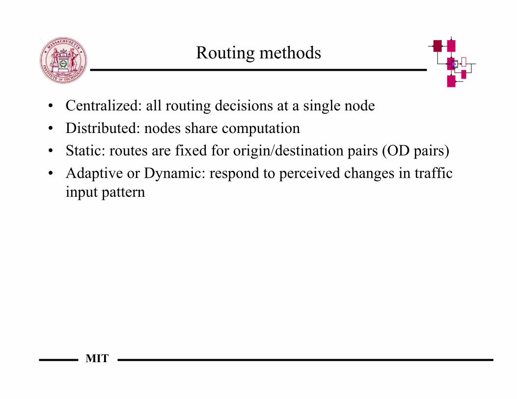
Routing methods
• Centralized: all routing decisions at a single node• Distributed: nodes share computation• Static: routes are fixed for origin/destination pairs (OD pairs)• Adaptive or Dynamic: respond to perceived changes in traffic
input pattern
MIT
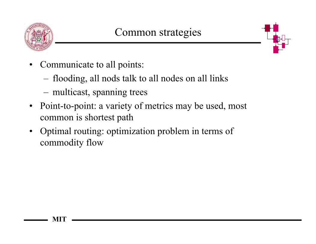
Common strategies
• Communicate to all points:– flooding, all nods talk to all nodes on all links– multicast, spanning trees
• Point-to-point: a variety of metrics may be used, mostcommon is shortest path
• Optimal routing: optimization problem in terms ofcommodity flow
MIT
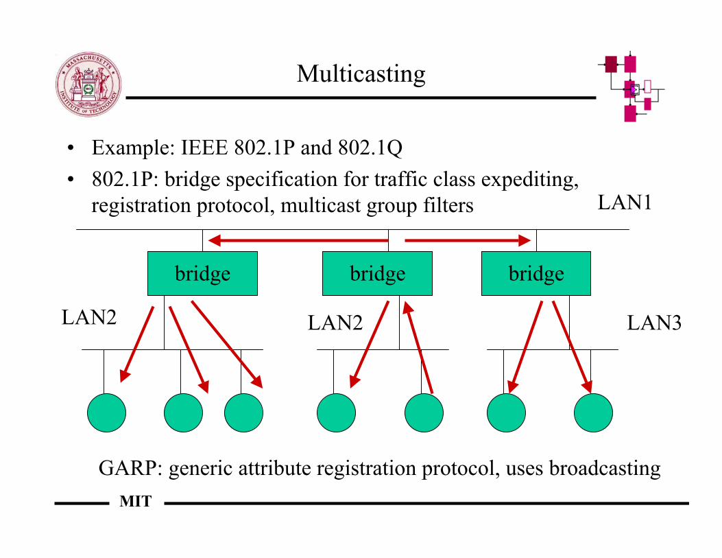
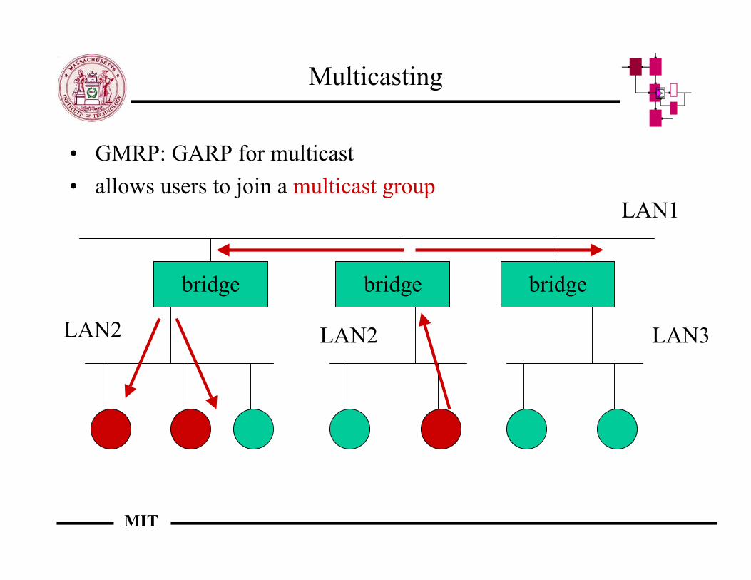
Multicasting
• Example: IEEE 802.1P and 802.1Q• 802.1P: bridge specification for traffic class expediting,
registration protocol, multicast group filters
bridge bridge bridge
GARP: generic attribute registration protocol, uses broadcasting
LAN2
LAN1
LAN2 LAN3
MIT
Multicasting
• GMRP: GARP for multicast• allows users to join a multicast group
bridge bridge bridge
LAN2
LAN1
LAN2 LAN3
MIT
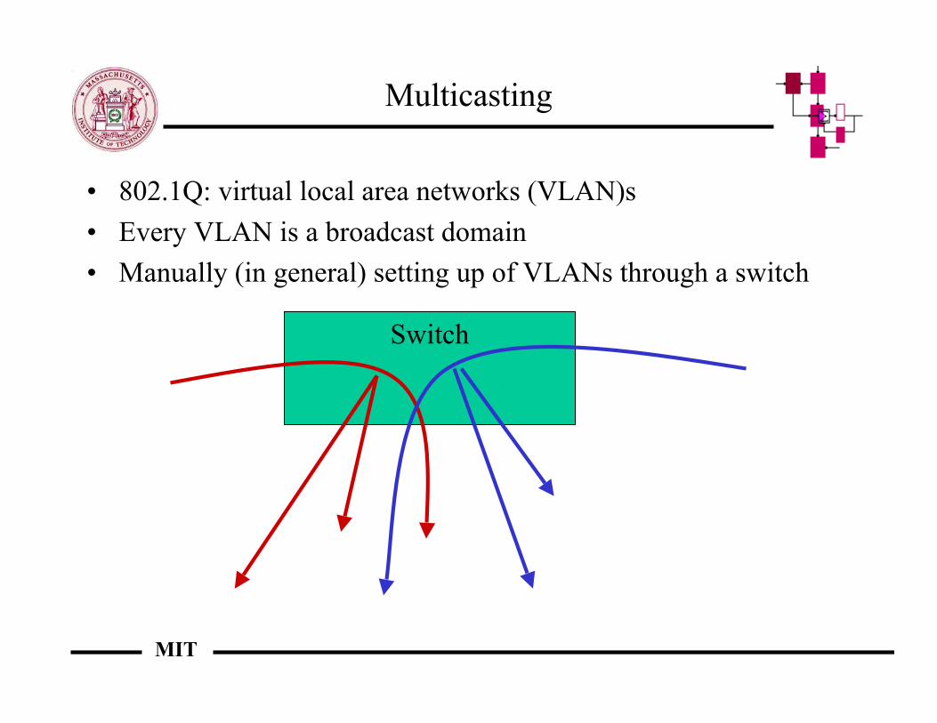
Multicasting
• 802.1Q: virtual local area networks (VLAN)s• Every VLAN is a broadcast domain• Manually (in general) setting up of VLANs through a switch
Switch
MIT
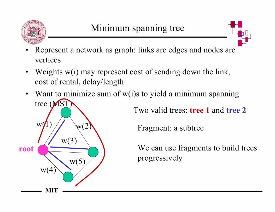
Minimum spanning tree
• Represent a network as graph: links are edges and nodes arevertices
• Weights w(i) may represent cost of sending down the link,cost of rental, delay/length
• Want to minimize sum of w(i)s to yield a minimum spanningtree (MST)
w(1) w(2)
w(3)
w(4)w(5)
Two valid trees: tree 1 and tree 2
Fragment: a subtree
We can use fragments to build trees progressively
root
MIT
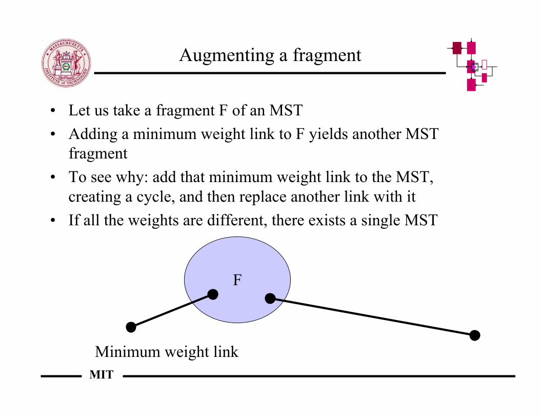
Augmenting a fragment
• Let us take a fragment F of an MST• Adding a minimum weight link to F yields another MST
fragment• To see why: add that minimum weight link to the MST,
creating a cycle, and then replace another link with it• If all the weights are different, there exists a single MST
F
Minimum weight link
MIT
Algorithms relying on augmenting fragments
• Prim-Dijkstra: start from the root node and graduallyaugment it until all nodes are in the MST
• Kruskal: every node is a fragment and fragments aresuccessively joined
• Example:
• The problem of multicast rather than broadcast is difficult -Steiner tree problem, NP-complete
1 2
4 6
7
3
8
910

MIT
Shortest Paths
• Interior gateway protocol• Option 1 (routing information protocol (RIP)):
– vector distance protocol: each gateway propagates a list of thenetworks it can reach and the distance to each network
– gateways use the list to compute new routes, then propagatetheir list of reachable networks
• Option 2 (open shortest path first (OSPF)):– link-state protocol: each gateway propagates status of its
individual connections to networks– protocol delivers each link state message to all other
participating gateways– if new link state information arrives, then gateway recomputes
next-hop along shortest path to each destination
MIT
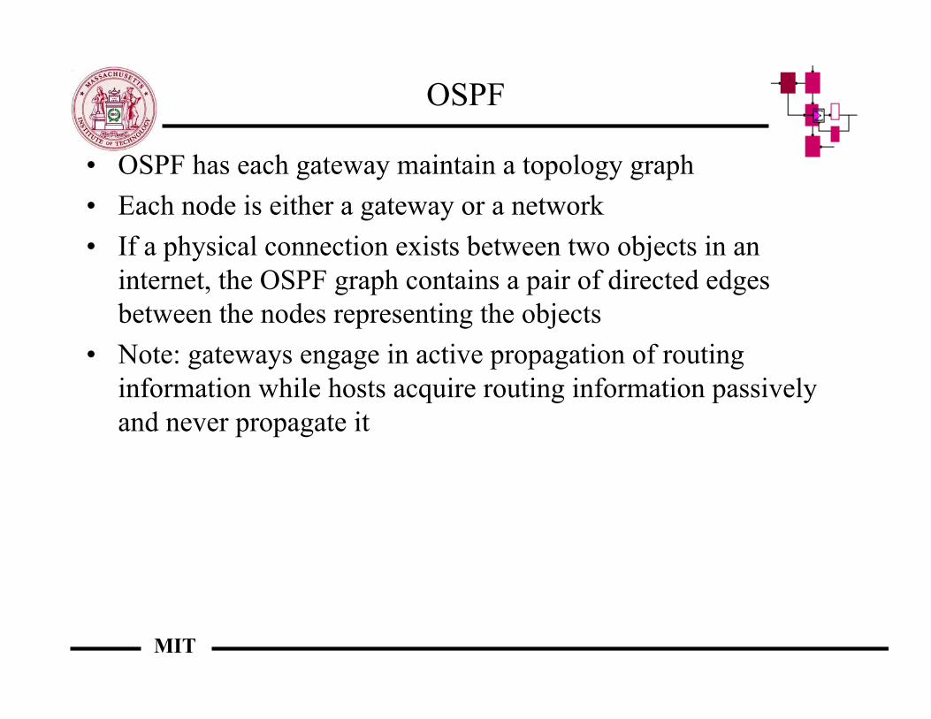
OSPF
• OSPF has each gateway maintain a topology graph• Each node is either a gateway or a network• If a physical connection exists between two objects in an
internet, the OSPF graph contains a pair of directed edgesbetween the nodes representing the objects
• Note: gateways engage in active propagation of routinginformation while hosts acquire routing information passivelyand never propagate it
MIT
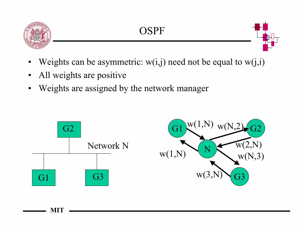
OSPF
• Weights can be asymmetric: w(i,j) need not be equal to w(j,i)• All weights are positive• Weights are assigned by the network manager
G1
G2
G3
Network N N
G2G1
G3
w(1,N)
w(1,N) w(N,2)
w(2,N)w(N,3)
w(3,N)
MIT
Shortest Path Algorithms
• Shortest path between two nodes: length = weight• Directed graphs (digraphs) (recall that MSTs were on undirected
graphs), edges are called arcs and have a direction (i,j) ≠ (j,i)• Shortest path problem: a directed path from A to B is a sequence of
distinct nodes A, n1, n2, …, nk, B, where (A, n1), (n1, n2), …,(nk, B) are directed arcs - find the shortest such path
• Variants of the problem: find shortest path from an origin to allnodes or from all nodes to an origin
• Assumption: all cycles have non-negative length• Three main algorithms:
– Dijsktra– Bellman-Ford– Floyd-Warshall
MIT
Dijkstra’s algorithm
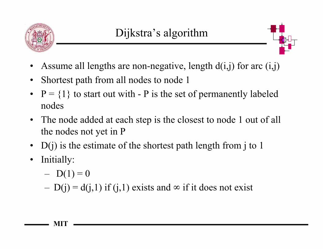
• Assume all lengths are non-negative, length d(i,j) for arc (i,j)• Shortest path from all nodes to node 1• P = {1} to start out with - P is the set of permanently labeled
nodes• The node added at each step is the closest to node 1 out of all
the nodes not yet in P• D(j) is the estimate of the shortest path length from j to 1• Initially:
– D(1) = 0– D(j) = d(j,1) if (j,1) exists and ∞ if it does not exist
MIT
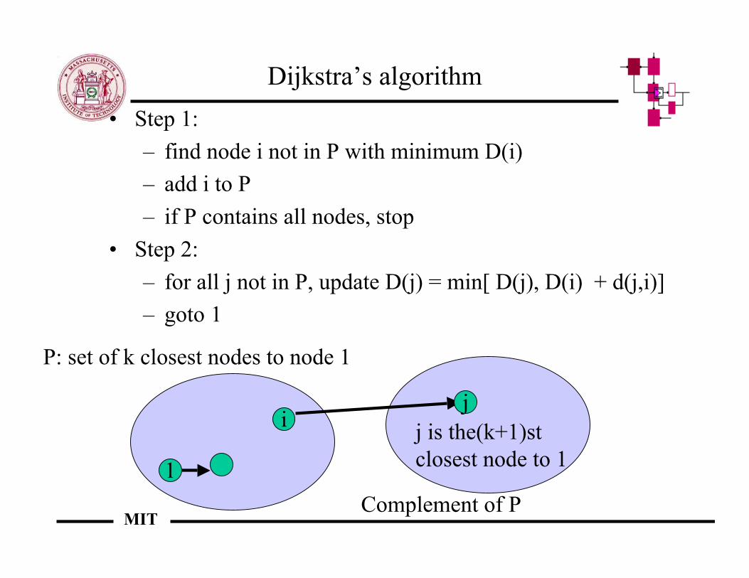
Dijkstra’s algorithm• Step 1:
– find node i not in P with minimum D(i)– add i to P– if P contains all nodes, stop
• Step 2:– for all j not in P, update D(j) = min[ D(j), D(i) + d(j,i)]– goto 1
1
ij
P: set of k closest nodes to node 1
Complement of P
j is the(k+1)st closest node to 1
MIT
Dijkstra
• At the beginning of each step 1,– D(j) is the shortest distance from j to 1 using nodes in 1
only (except j may possibly be outside P)– D(i) ≤ D(j) when i is on p and j is not in P
• How long does is take to run?– We go through step 1and 2 roughly N times, where N is
the number of nodes– we go through roughly N computations at each step 2– time complexity is thus O(N2)– Note: to be more precise, we would have to take into
account the maximum size d of the lengths and the timecomplexity would depend on log(d)
MIT
Bellman-Ford
• Allows negative lengths, but not negative cycles• B-F works at looking at negative lengths from every node to
node 1• If arc (i,j) does not exist, we set d(i,j) to infinity• We look at walks: consider the shortest walk from node i to 1
after at most h arcs• Algorithm:
– Dh+1(i) = minover all j[d(i,j) + Dh(i)]for all i other than 1– we terminate when Dh+1(i) = Dh(i)
• The Dh+1(i) are the lengths of the shortest path from i to 1with no more than h arcs in it

MIT
Bellman-Ford
• Let us show this by induction– D1(i) = d(i,1)for every i other than 1, since one hop corresponds
to having a single arc– now suppose this holds for some h, let us show it for h+1: we
assume that for all k ≤ h, Dk(i) is the length of the shortest walkfrom i to 1 with k arcs or fewer
– minover all j[d(i,j) + Dh(i)] allows up to h+1 arcs, but Dh(i) wouldhave fewer than h arcs, so min[Dh(i), minover all j[d(i,j) + Dh(i)]]= Dh+1(i)
• Time complexity: A, where A is the number of arcs, for at most N-1 nodes (note: A can be up to (N-1)2 )
• In practice, B-F still often performs better than Dijkstra
MIT
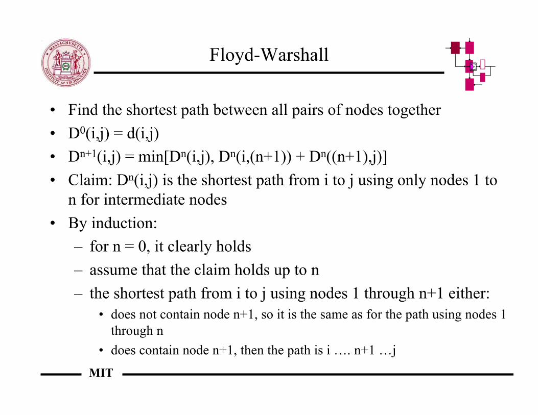
Floyd-Warshall
• Find the shortest path between all pairs of nodes together• D0(i,j) = d(i,j)• Dn+1(i,j) = min[Dn(i,j), Dn(i,(n+1)) + Dn((n+1),j)]• Claim: Dn(i,j) is the shortest path from i to j using only nodes 1 to
n for intermediate nodes• By induction:
– for n = 0, it clearly holds– assume that the claim holds up to n– the shortest path from i to j using nodes 1 through n+1 either:
• does not contain node n+1, so it is the same as for the path using nodes 1through n
• does contain node n+1, then the path is i …. n+1 …j
MIT
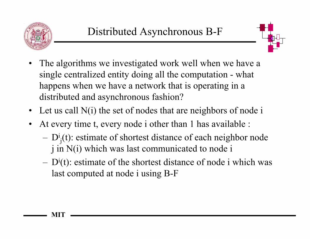
Distributed Asynchronous B-F
• The algorithms we investigated work well when we have asingle centralized entity doing all the computation - whathappens when we have a network that is operating in adistributed and asynchronous fashion?
• Let us call N(i) the set of nodes that are neighbors of node i• At every time t, every node i other than 1 has available :
– Dij(t): estimate of shortest distance of each neighbor node
j in N(i) which was last communicated to node i– Di(t): estimate of the shortest distance of node i which was
last computed at node i using B-F
MIT
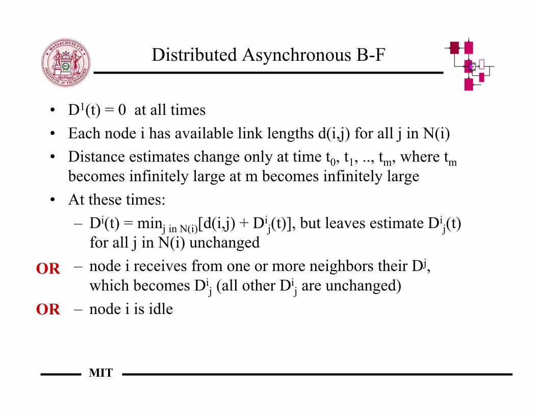
Distributed Asynchronous B-F
• D1(t) = 0 at all times• Each node i has available link lengths d(i,j) for all j in N(i)• Distance estimates change only at time t0, t1, .., tm, where tm
becomes infinitely large at m becomes infinitely large• At these times:
– Di(t) = minj in N(i)[d(i,j) + Dij(t)], but leaves estimate Di
j(t)for all j in N(i) unchanged
– node i receives from one or more neighbors their Dj,which becomes Di
j (all other Dij are unchanged)
– node i is idle
OR
OR
MIT
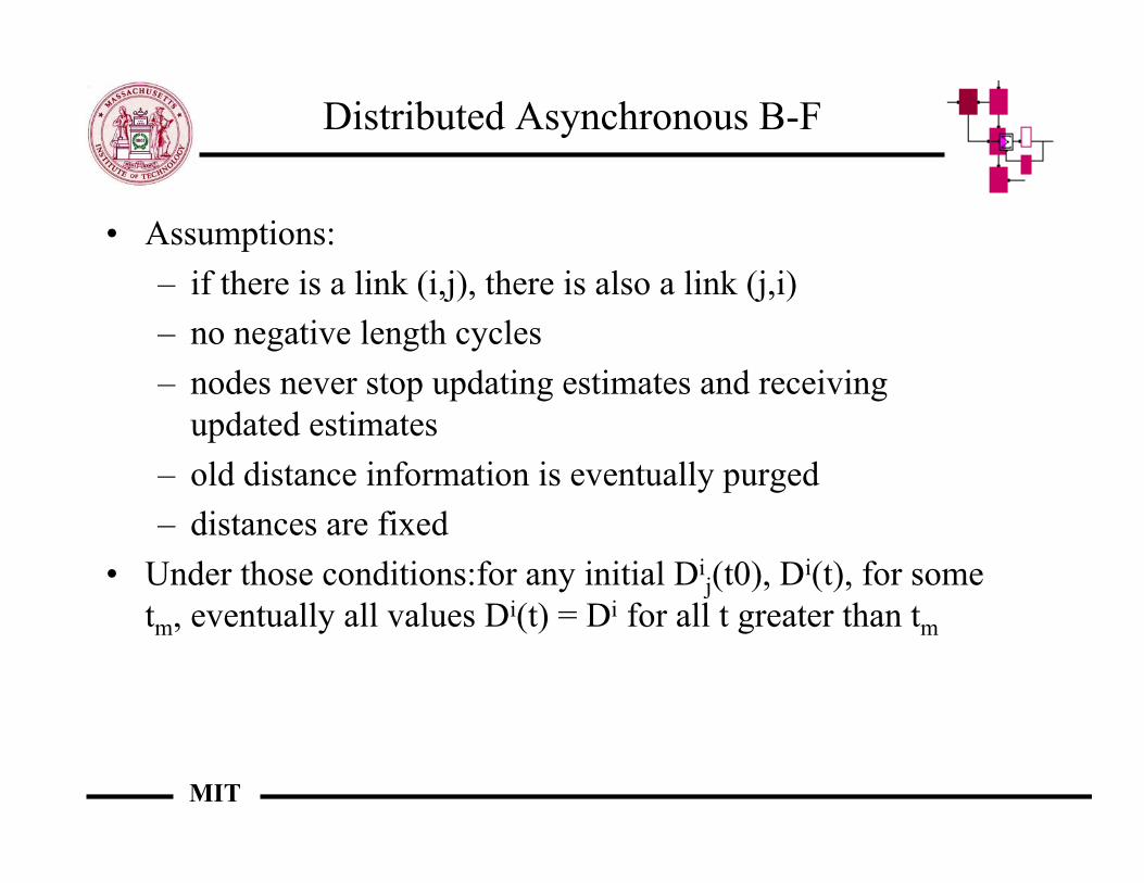
Distributed Asynchronous B-F
• Assumptions:– if there is a link (i,j), there is also a link (j,i)– no negative length cycles– nodes never stop updating estimates and receiving
updated estimates– old distance information is eventually purged– distances are fixed
• Under those conditions:for any initial Dij(t0), Di(t), for some
tm, eventually all values Di(t) = Di for all t greater than tm
MIT
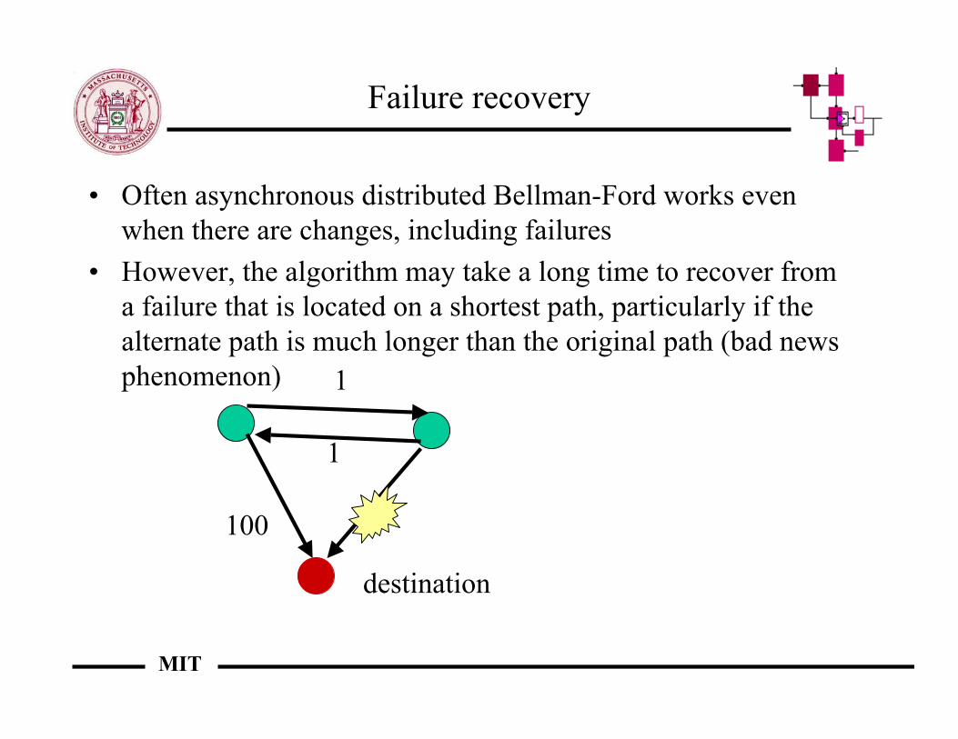
Failure recovery
• Often asynchronous distributed Bellman-Ford works evenwhen there are changes, including failures
• However, the algorithm may take a long time to recover froma failure that is located on a shortest path, particularly if thealternate path is much longer than the original path (bad newsphenomenon)
destination
1
1
100
MIT
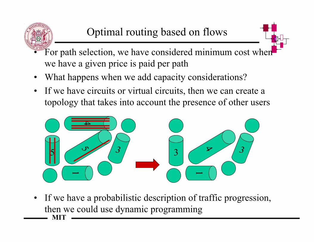
Optimal routing based on flows
• For path selection, we have considered minimum cost whenwe have a given price is paid per path
• What happens when we add capacity considerations?• If we have circuits or virtual circuits, then we can create a
topology that takes into account the presence of other users
• If we have a probabilistic description of traffic progression,then we could use dynamic programming
5 3
14
5
3 3
14
MIT
Routing based on flows
• When we have packets or fine granularity virtual circuits(VCs), we can assume that we have roughly fluid flows
• We will try to optimize a cost function related to the flowF(i,j) (arrival rate in terms of of what we may be considering)on the link (i,j)
• A reasonable metric is
where D is some monotonically increasing function thatgrows very sharply when F(i,j) approaches the link capacity
• These type of models are called flow models - they look onlyat mean flow, they do not consider higher moments
j))D(F(i,j)(i,!
MIT
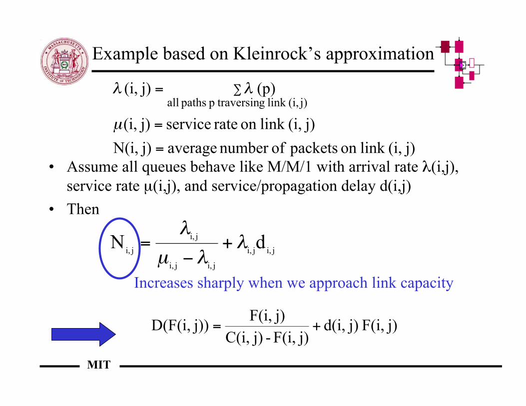
Example based on Kleinrock’s approximation
• Assume all queues behave like M/M/1 with arrival rate λ(i,j),service rate µ(i,j), and service/propagation delay d(i,j)
• Then
ji,ji,
ji,ji,
ji,
ji,dN !
!µ
!+
"=
j)F(i, j)d(i,j)F(i,-j)C(i,
j)F(i,j))D(F(i, +=
Increases sharply when we approach link capacity
j)(i,link on packets ofnumber averagej)N(i,
j)(i,link on rate servicej)(i,
(p)j)(i,j)(i,link g traversinp paths all
=
=
= !
µ
""
MIT
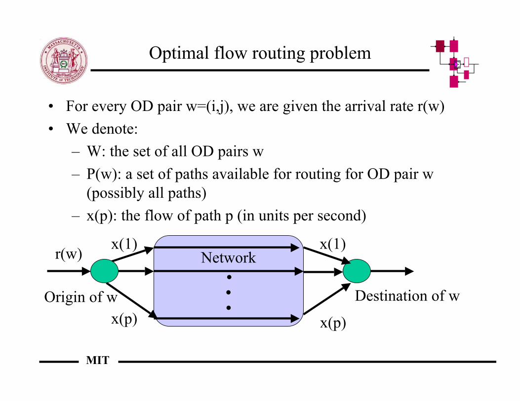
Optimal flow routing problem
• For every OD pair w=(i,j), we are given the arrival rate r(w)• We denote:
– W: the set of all OD pairs w– P(w): a set of paths available for routing for OD pair w
(possibly all paths)– x(p): the flow of path p (in units per second)
..
.Networkr(w)
Origin of w Destination of w
x(1)
x(p)
x(1)
x(p)
MIT
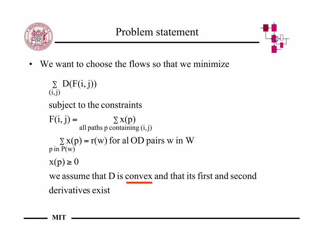
Problem statement
• We want to choose the flows so that we minimize
exist sderivative
second andfirst its that andconvex is D that assume we
0 x(p)
in W wpairs OD alfor r(w) x(p)
x(p) j)F(i,
sconstraint thesubject to
j))D(F(i,
P(w)in p
j)(i, containing p paths all
j)(i,
!
=
=
"
"
"
MIT
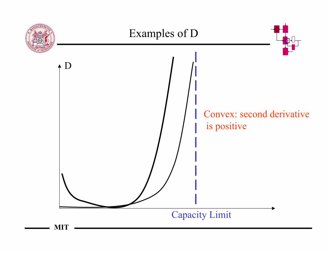
Examples of D
Capacity Limit
D
Convex: second derivative is positive
MIT
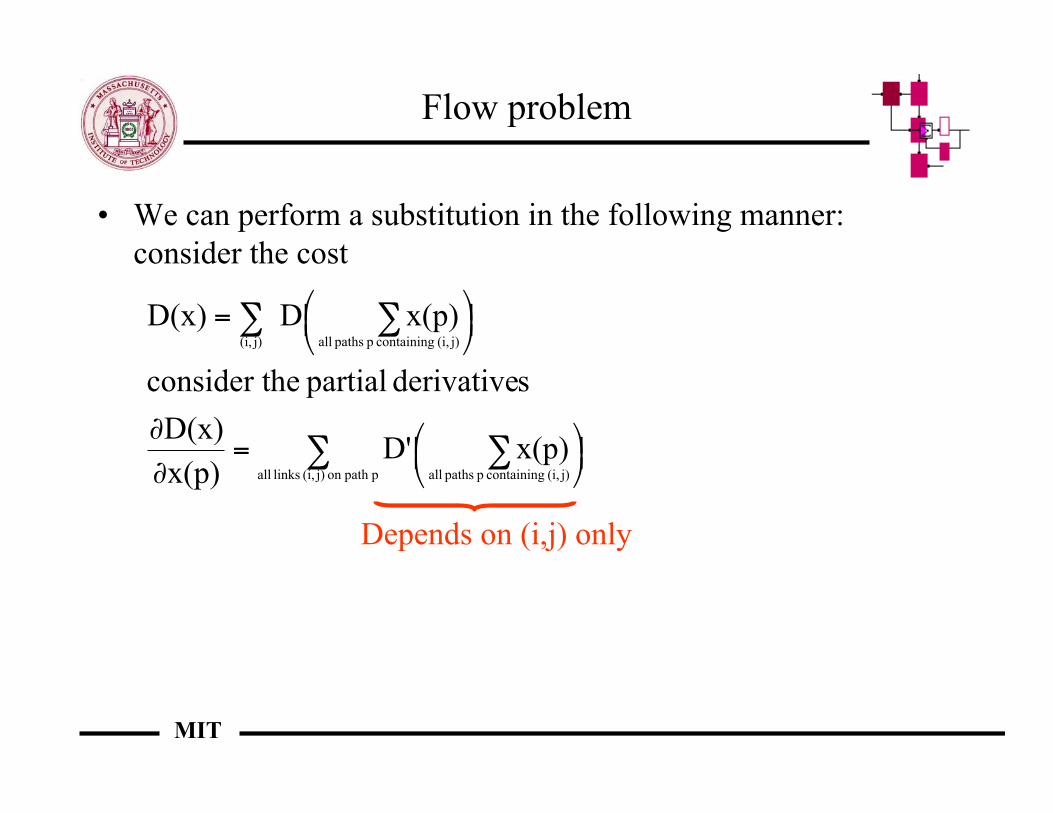
Flow problem
• We can perform a substitution in the following manner:consider the cost
! !
!!
"#$%
&'=
(
(
"#$%
&'=
ppath on j)(i, links all j)(i, containing p paths all
j)(i, containing p paths allj)(i,
x(p)D'x(p)
D(x)
sderivative partial heconsider t
x(p)DD(x)
Depends on (i,j) only
MIT
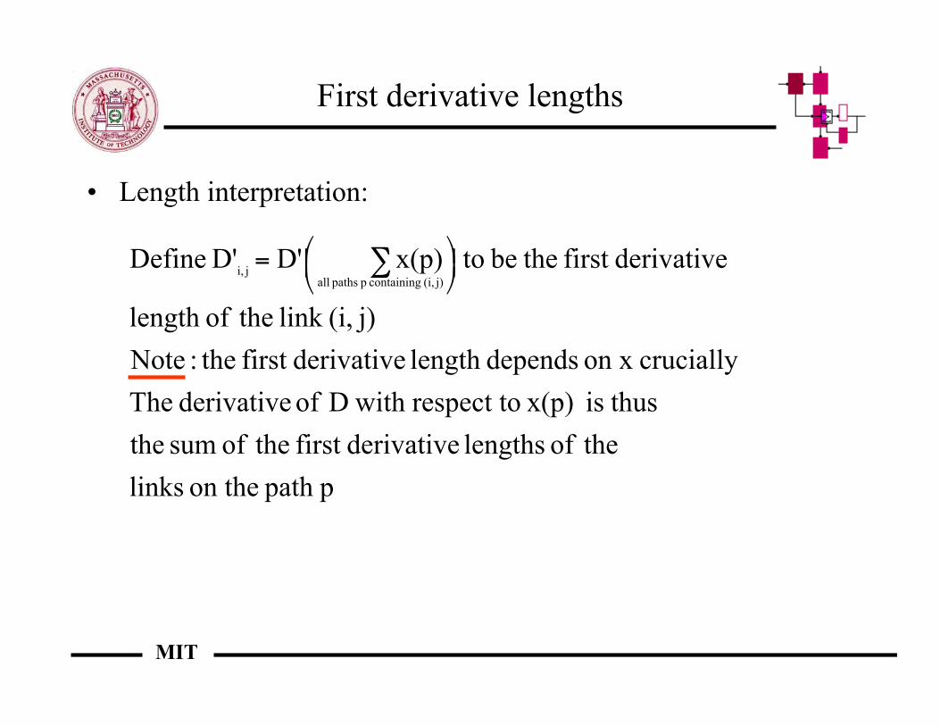
First derivative lengths
• Length interpretation:
ppath on the links
theof lengths derivativefirst theof sum the
thusis x(p)respect to with D of derivative The
cruciallyon x dependslength derivativefirst the:Note
j)(i,link theoflength
derivativefirst thebe tox(p)D'D' Definej)(i, containing p paths all
ji, !"#$
%&= '
MIT
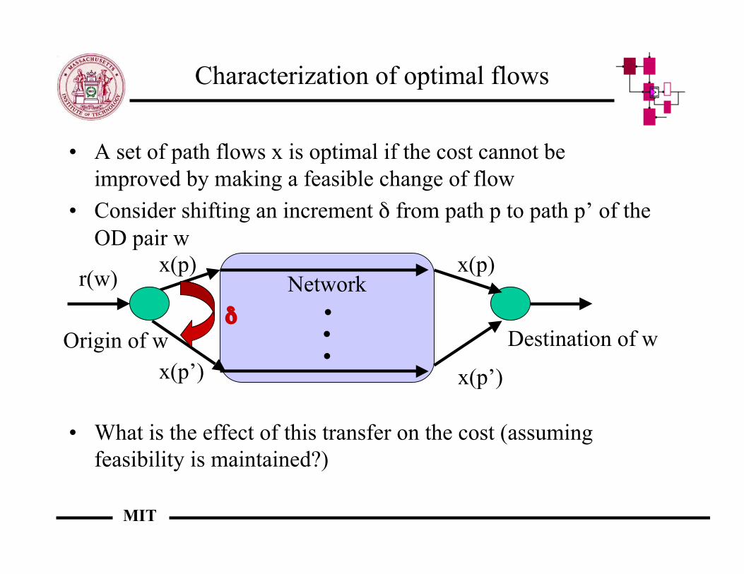
Characterization of optimal flows
• A set of path flows x is optimal if the cost cannot beimproved by making a feasible change of flow
• Consider shifting an increment δ from path p to path p’ of theOD pair w
• What is the effect of this transfer on the cost (assumingfeasibility is maintained?)
..
.Networkr(w)
Origin of w Destination of w
x(p)
x(p’)
x(p)
x(p’)
δ
MIT
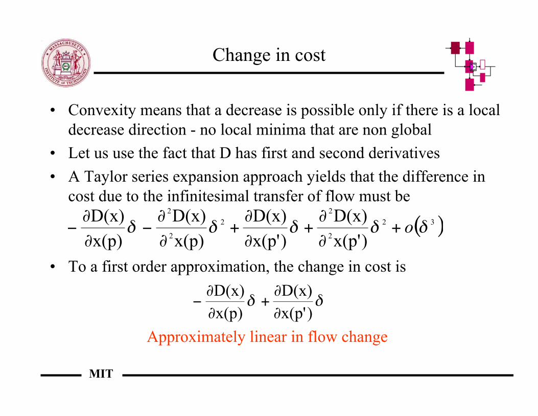
Change in cost
• Convexity means that a decrease is possible only if there is a localdecrease direction - no local minima that are non global
• Let us use the fact that D has first and second derivatives• A Taylor series expansion approach yields that the difference in
cost due to the infinitesimal transfer of flow must be
• To a first order approximation, the change in cost is
!!)x(p'
D(x)
x(p)
D(x)
"
"+
"
"#
( )32
2
2
2
2
2
)x(p'
D(x)
)x(p'
D(x)
x(p)
D(x)
x(p)
D(x)!!!!! o+
"
"+
"
"+
"
"#
"
"#
Approximately linear in flow change
MIT
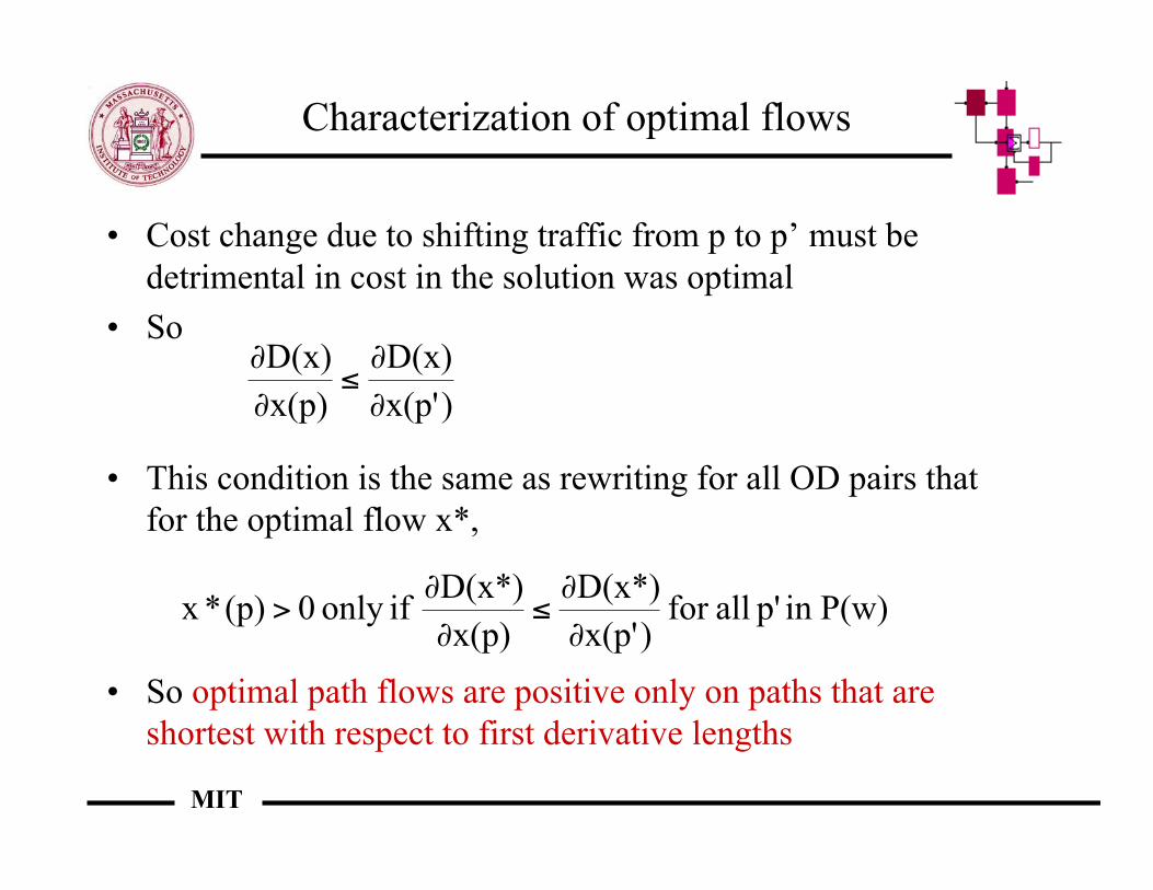
Characterization of optimal flows
• Cost change due to shifting traffic from p to p’ must bedetrimental in cost in the solution was optimal
• So
• This condition is the same as rewriting for all OD pairs thatfor the optimal flow x*,
• So optimal path flows are positive only on paths that areshortest with respect to first derivative lengths
)x(p'
D(x)
x(p)
D(x)
!
!"
!
!
P(w)in p' allfor )x(p'
D(x*)
x(p)
D(x*) ifonly 0 (p)*x
!
!"
!
!>
MIT
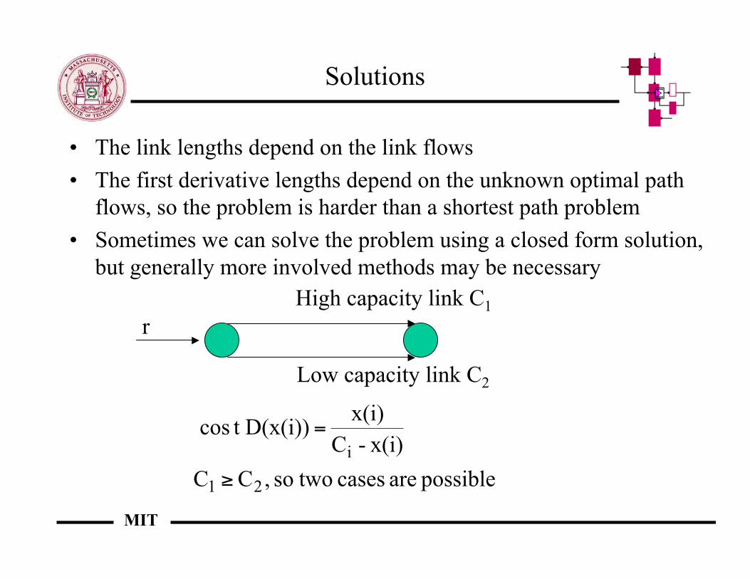
Solutions
• The link lengths depend on the link flows• The first derivative lengths depend on the unknown optimal path
flows, so the problem is harder than a shortest path problem• Sometimes we can solve the problem using a closed form solution,
but generally more involved methods may be necessary
rHigh capacity link C1
Low capacity link C2
possible are cases twoso ,C C
x(i)- C
x(i) D(x(i))t cos
21
i
!
=
MIT
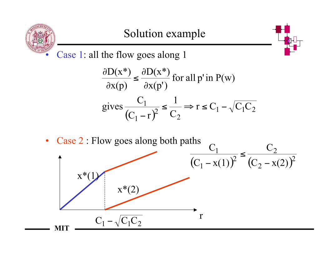
Solution example
• Case 1: all the flow goes along 1
• Case 2 : Flow goes along both paths
( )211
22
1
1 CCCrC
1
rC
C gives
P(w)in p' allfor )x(p'
D(x*)
x(p)
D(x*)
!"#"!
$
$"
$
$
( ) ( )22
22
1
1
x(2)C
C
x(1)C
C
!"
!
211 CCC !r
x*(1)x*(2)
MIT
Solution methods
• In general finding solutions may be difficult and differenttypes of methods may need to be applied
• Reduce cost while maintaining feasibility• A common theme in the methods for improving solutions is
to perturb current solution in a way that is feasible andreduces cost
• Why not just use minimum first derivative lengths (MFDLs)?• Lengths are dependent on flow values x, so search is in
general difficult and can lead to instability
MIT
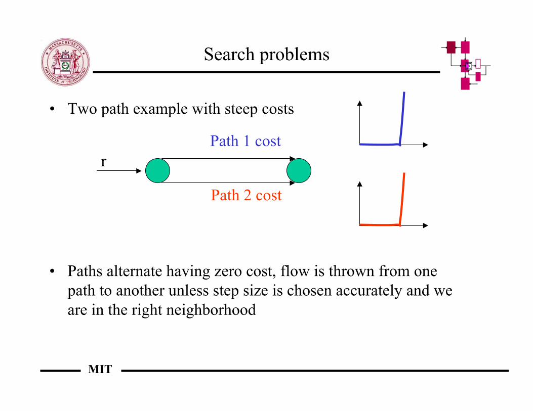
Search problems
• Two path example with steep costs
• Paths alternate having zero cost, flow is thrown from onepath to another unless step size is chosen accurately and weare in the right neighborhood
rPath 1 cost
Path 2 cost
MIT
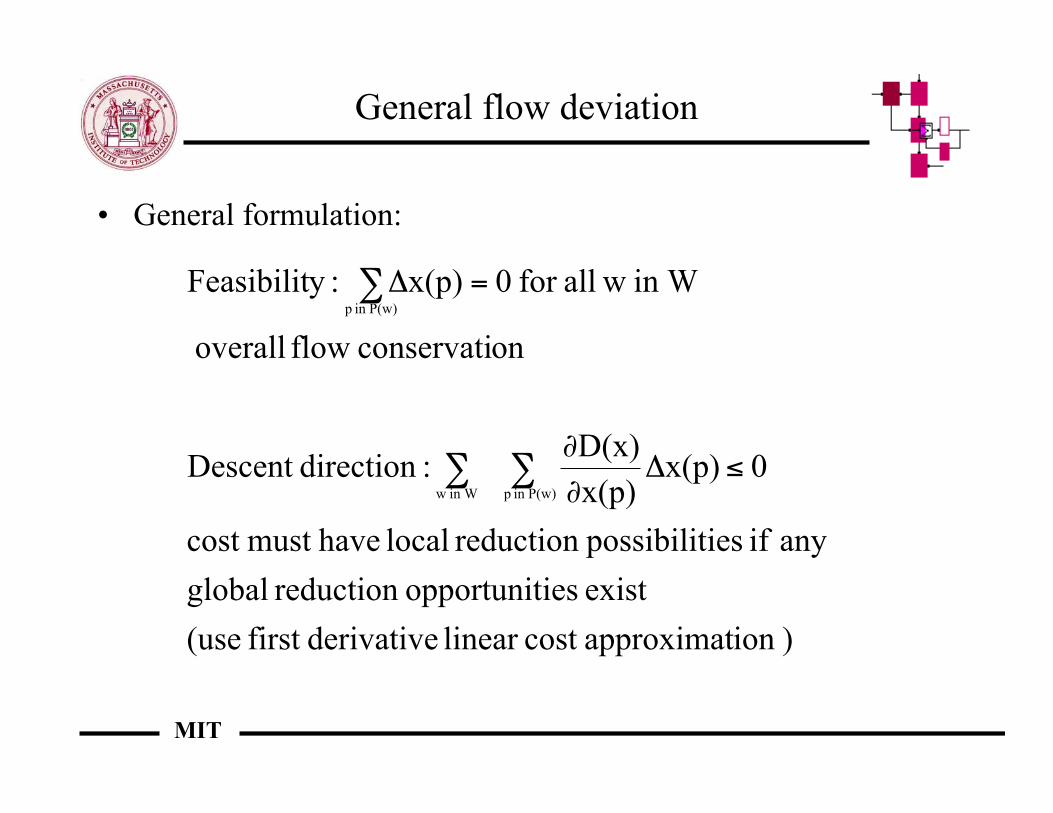
General flow deviation
• General formulation:
)ion approximatcost linear derivativefirst (use
exist iesopportunitreduction global
any if iespossibilitreduction local havemust cost
0 x(p)x(p)
D(x) :directionDescent
onconservati flow overall
in W wallfor 0x(p):yFeasibilit
P(w)in p in W w
P(w)in p
!"#
#
="
$$
$
MIT
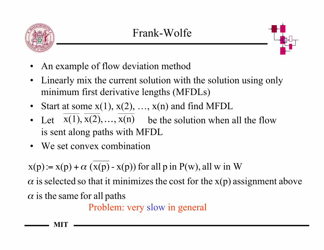
Frank-Wolfe
• An example of flow deviation method• Linearly mix the current solution with the solution using only
minimum first derivative lengths (MFDLs)• Start at some x(1), x(2), …, x(n) and find MFDL• Let be the solution when all the flow
is sent along paths with MFDL• We set convex combination
x(n) , ,x(2) ,x(1) …
paths allfor same theis
above assignment x(p)for thecost theminimizesit that so selected is
in W wall P(w),in p allfor x(p))- x(p)( x(p): x(p)
!
!
!+=
Problem: very slow in general
MIT
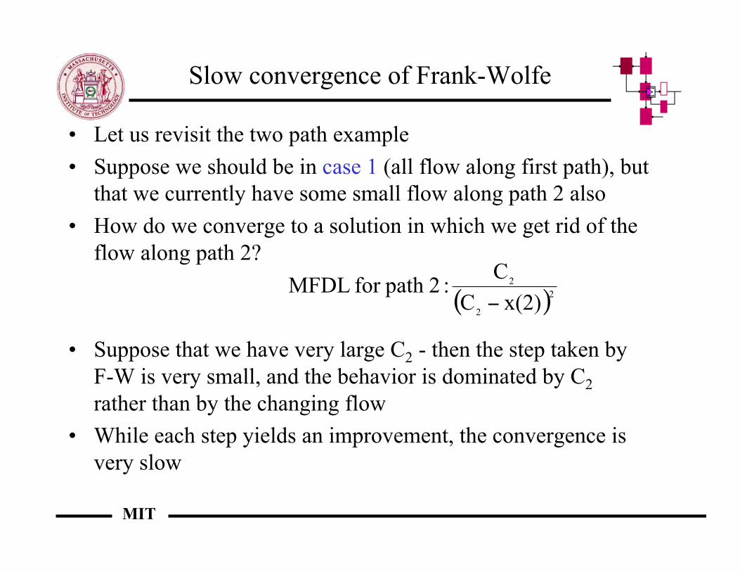
Slow convergence of Frank-Wolfe
• Let us revisit the two path example• Suppose we should be in case 1 (all flow along first path), but
that we currently have some small flow along path 2 also• How do we converge to a solution in which we get rid of the
flow along path 2?
• Suppose that we have very large C2 - then the step taken byF-W is very small, and the behavior is dominated by C2rather than by the changing flow
• While each step yields an improvement, the convergence isvery slow
( )22
2
x(2)C
C :2path for MFDL
!
MIT
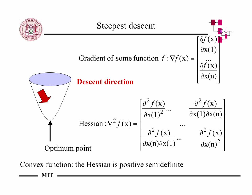
Steepest descent
Optimum point
Convex function: the Hessian is positive semidefinite
!!!!!!
"
#
$$$$$$
%
&
'
'
''
'
''
'
'
'
=(
!!!!!
"
#
$$$$$
%
&
'
'
'
'
=(
2
22
2
2
2
2
x(n)
)x(...
x(1)x(n)
)x(
...
x(n)x(1)
)x(...
x(1)
)x(
)x( :Hessian
x(n)
)x(...
x(1)
)x(
)x( :function some ofGradient
ff
ff
f
f
f
ff
Descent direction
MIT
Outline
• Rerouting• Path-based recovery• Rings• Beyond rings• Beyond rerouting : codes
MIT
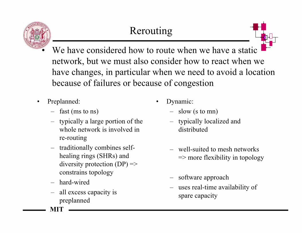
Rerouting
• We have considered how to route when we have a staticnetwork, but we must also consider how to react when wehave changes, in particular when we need to avoid a locationbecause of failures or because of congestion
• Preplanned:– fast (ms to ns)– typically a large portion of the
whole network is involved inre-routing
– traditionally combines self-healing rings (SHRs) anddiversity protection (DP) =>constrains topology
– hard-wired– all excess capacity is
preplanned
• Dynamic:– slow (s to mn)– typically localized and
distributed
– well-suited to mesh networks=> more flexibility in topology
– software approach– uses real-time availability of
spare capacity
MIT
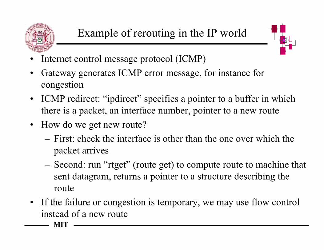
Example of rerouting in the IP world
• Internet control message protocol (ICMP)• Gateway generates ICMP error message, for instance for
congestion• ICMP redirect: “ipdirect” specifies a pointer to a buffer in which
there is a packet, an interface number, pointer to a new route• How do we get new route?
– First: check the interface is other than the one over which thepacket arrives
– Second: run “rtget” (route get) to compute route to machine thatsent datagram, returns a pointer to a structure describing theroute
• If the failure or congestion is temporary, we may use flow controlinstead of a new route

MIT
Rerouting for ATM
• ATM is part datagram, part circuit oriented, so recoverymethods span many different types
• Dynamic methods release connections and then seek ways ofre-establishing them: not necessarily per VP or VC approach– private network to network interface (PNNI) crankback– distributed restoration algorithms (DRAs)
• Circuit-oriented methods often have preplanned componentand work on a per VC, VP basis– dedicated shared VPs, VCs or soft VPs, VCs
MIT
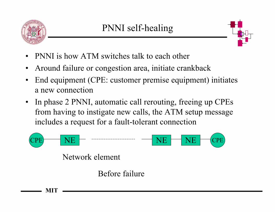
PNNI self-healing
• PNNI is how ATM switches talk to each other• Around failure or congestion area, initiate crankback• End equipment (CPE: customer premise equipment) initiates
a new connection• In phase 2 PNNI, automatic call rerouting, freeing up CPEs
from having to instigate new calls, the ATM setup messageincludes a request for a fault-tolerant connection
NE NE NECPE CPE
Network element
Before failure
MIT
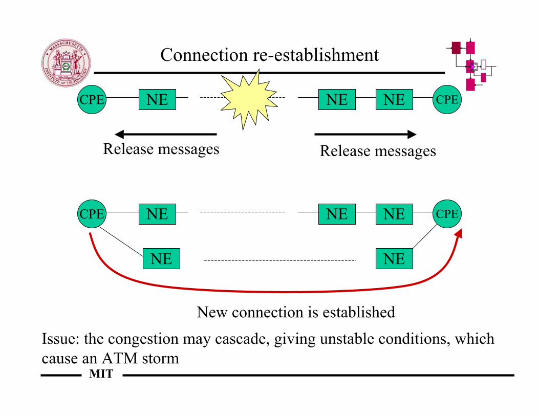
Connection re-establishment
NE NE NECPE CPE
Release messages Release messages
NE NE NECPE CPE
NE NE
New connection is establishedIssue: the congestion may cascade, giving unstable conditions, whichcause an ATM storm
MIT
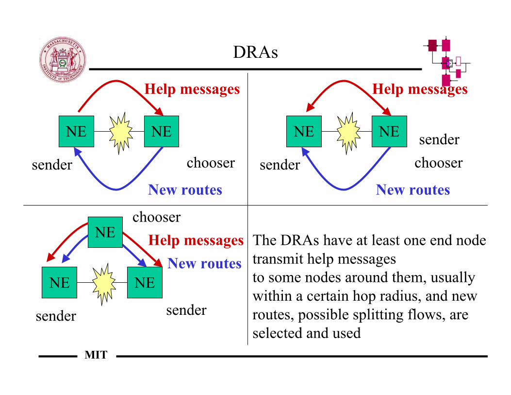
DRAs
NE NE
sender chooser
Help messages
New routes
NE NE
sender chooser
Help messages
New routes
sender
NE NE
sender
New routes
sender
chooserHelp messagesNE The DRAs have at least one end node
transmit help messagesto some nodes around them, usuallywithin a certain hop radius, and new routes, possible splitting flows, are selected and used
MIT
Circuit-oriented methods
• Circuit-oriented methods seek to replace a route with anotherone, whether end-to-end or over some portion that is affectedby a failure
• Several issues arise:– How do we perform recovery in a bandwidth-efficient
manner– How does recovery interface with network management– What sort of granularity do we need– What happens when a node rather than a link fails
MIT
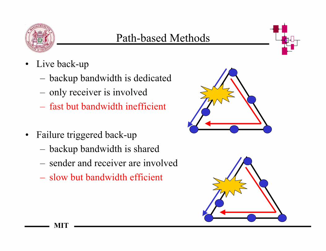
Path-based Methods
• Live back-up– backup bandwidth is dedicated– only receiver is involved– fast but bandwidth inefficient
• Failure triggered back-up– backup bandwidth is shared– sender and receiver are involved– slow but bandwidth efficient
MIT
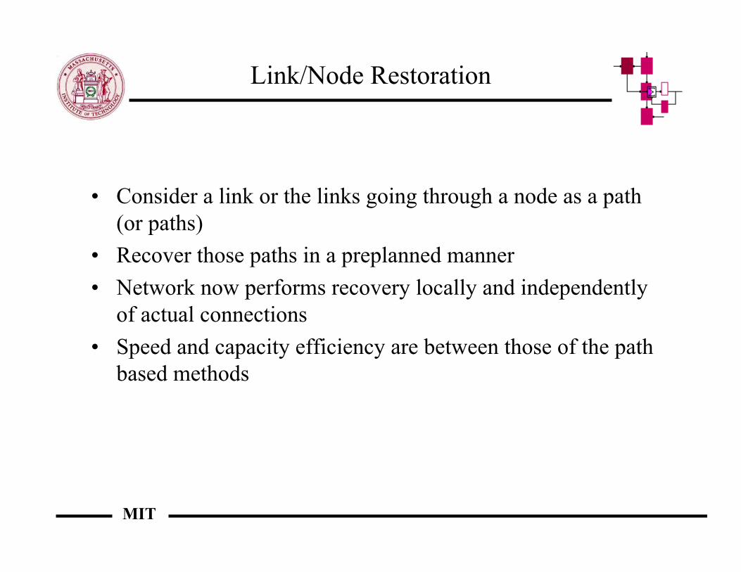
Link/Node Restoration
• Consider a link or the links going through a node as a path(or paths)
• Recover those paths in a preplanned manner• Network now performs recovery locally and independently
of actual connections• Speed and capacity efficiency are between those of the path
based methods
MIT
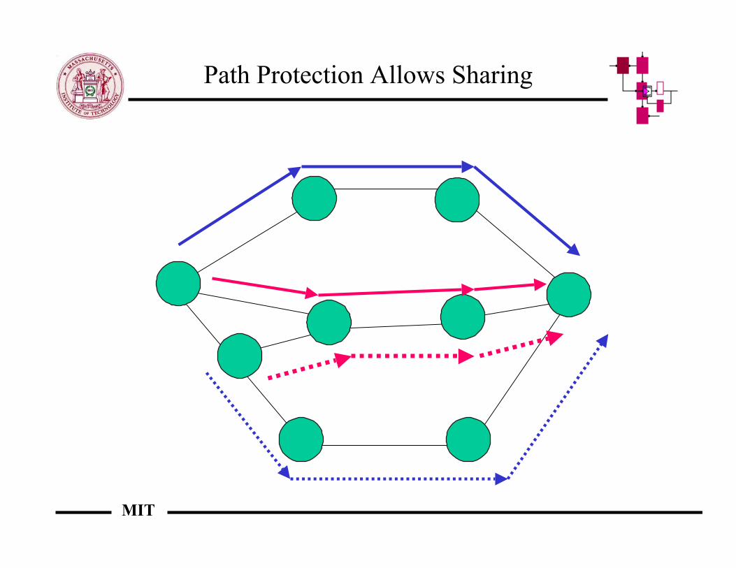
Path Protection Allows Sharing
MIT
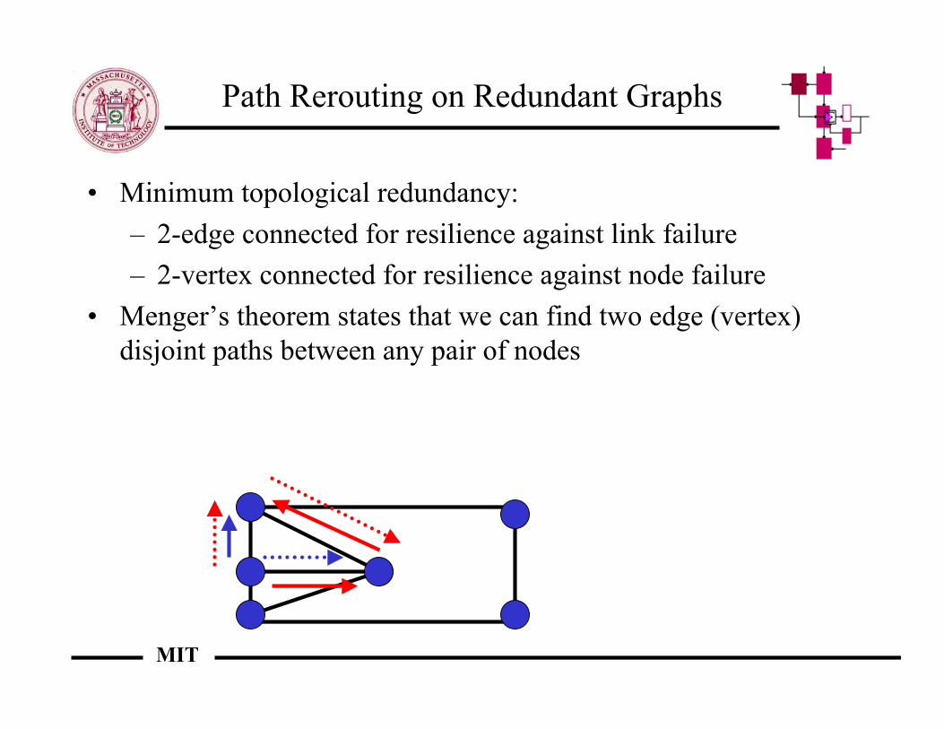
Path Rerouting on Redundant Graphs
• Minimum topological redundancy:– 2-edge connected for resilience against link failure– 2-vertex connected for resilience against node failure
• Menger’s theorem states that we can find two edge (vertex)disjoint paths between any pair of nodes
MIT
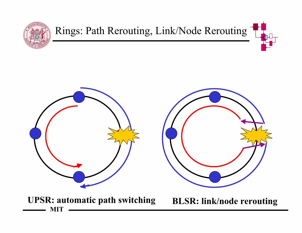
Rings: Path Rerouting, Link/Node Rerouting
UPSR: automatic path switching BLSR: link/node rerouting
MIT
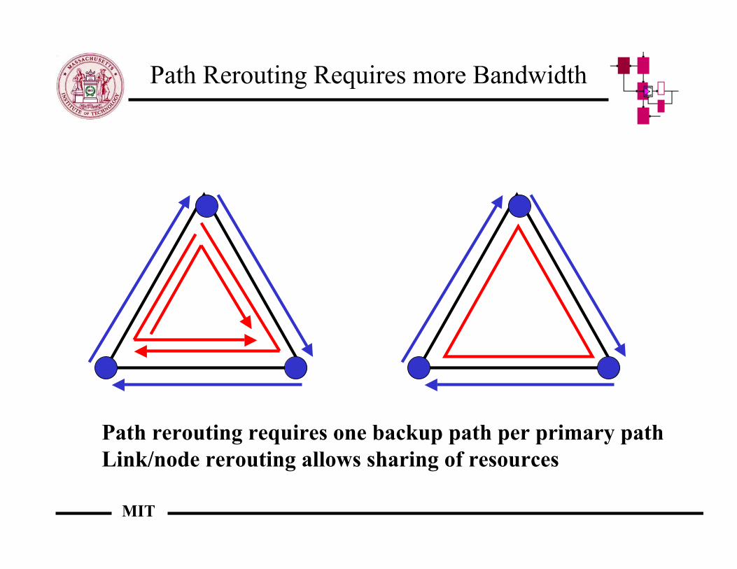
Path Rerouting Requires more Bandwidth
Path rerouting requires one backup path per primary pathLink/node rerouting allows sharing of resources
MIT
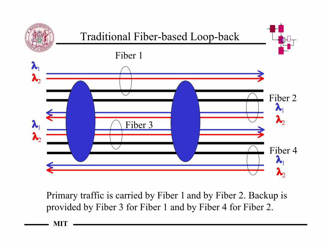
Traditional Fiber-based Loop-back
λ1λ2
λ1λ2
Fiber 1
Fiber 2
Primary traffic is carried by Fiber 1 and by Fiber 2. Backup isprovided by Fiber 3 for Fiber 1 and by Fiber 4 for Fiber 2.
λ1λ2
λ1λ2
Fiber 3
Fiber 4
MIT
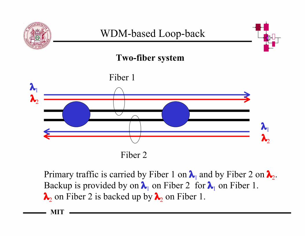
WDM-based Loop-back
λ1λ2
λ1λ2
Fiber 1
Fiber 2
Primary traffic is carried by Fiber 1 on λ1 and by Fiber 2 on λ2.Backup is provided by on λ1 on Fiber 2 for λ1 on Fiber 1. λ2 on Fiber 2 is backed up by λ2 on Fiber 1.
Two-fiber system
MIT
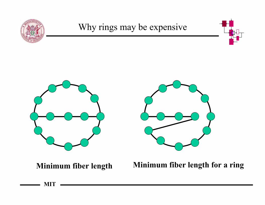
Why rings may be expensive
Minimum fiber length Minimum fiber length for a ring
MIT
Covers of Rings
• Usual method for applying preplanned recovery to meshnetworks
• UPSR style covers: minimum cycle cover is NP completeproblem (conjectured by Itai, Lipton, Papadimitriou andRodeh, shown by Thomassen)
• BLSR style covers: double cycle cover conjecture (seeJaeger, applied to restoration by Ellinas, Stern andHailemariam)
• Hierarchical Rings (Shi and Fonseka)• Is there a fundamental reason for rings?
MIT
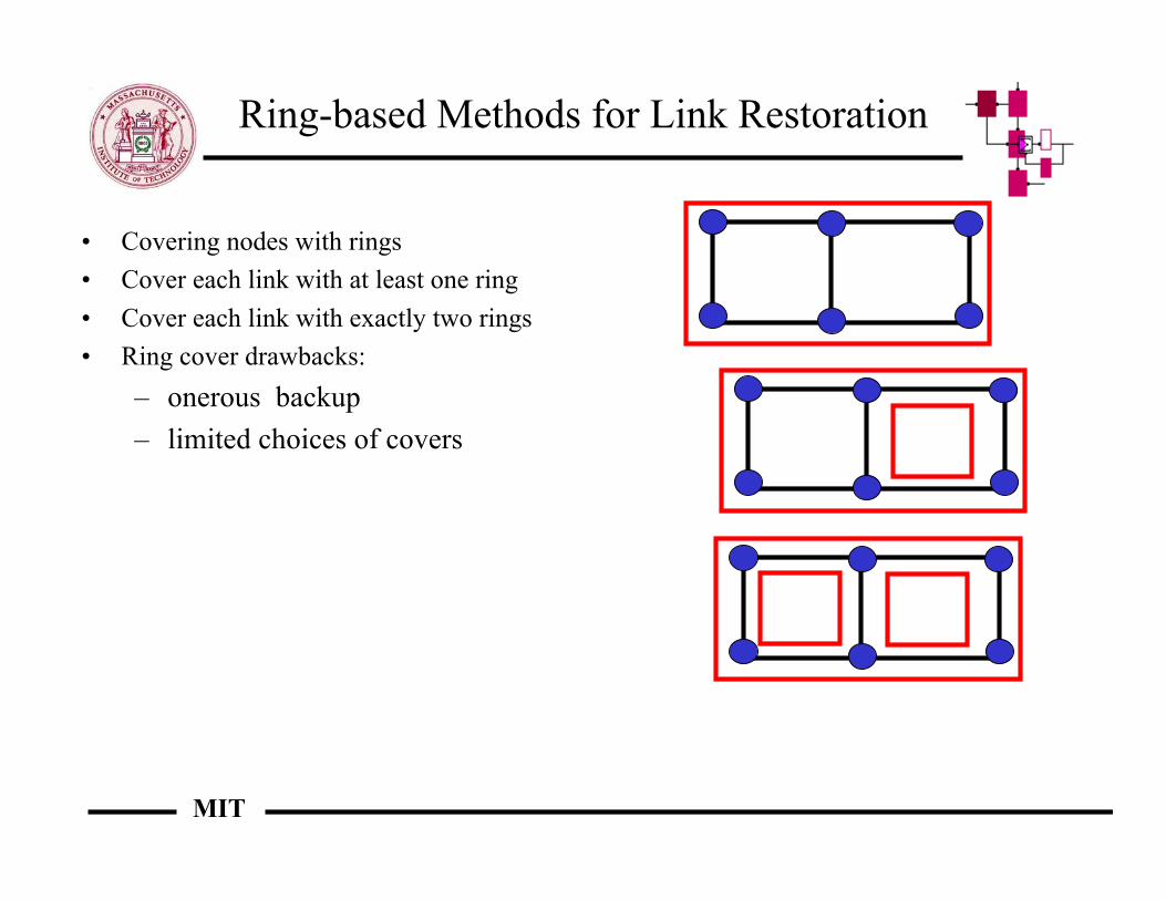
Ring-based Methods for Link Restoration
• Covering nodes with rings• Cover each link with at least one ring• Cover each link with exactly two rings• Ring cover drawbacks:
– onerous backup– limited choices of covers
MIT
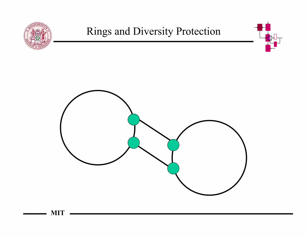
Rings and Diversity Protection
MIT
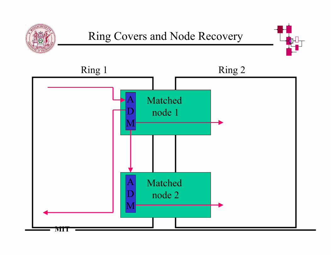
Ring Covers and Node Recovery
Matched node 1
Matched node 2
ADM
ADM
Ring 2Ring 1
MIT
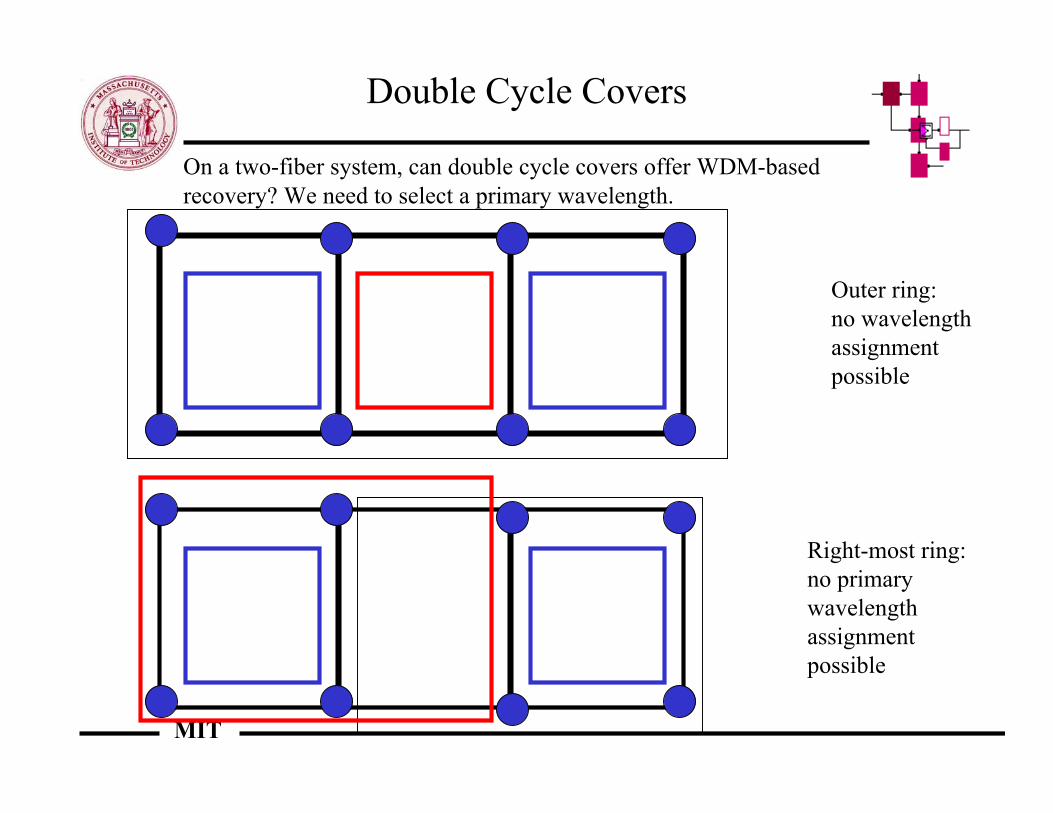
Double Cycle Covers
Outer ring:no wavelengthassignmentpossible
Right-most ring:no primarywavelength assignment possible
On a two-fiber system, can double cycle covers offer WDM-basedrecovery? We need to select a primary wavelength.
MIT
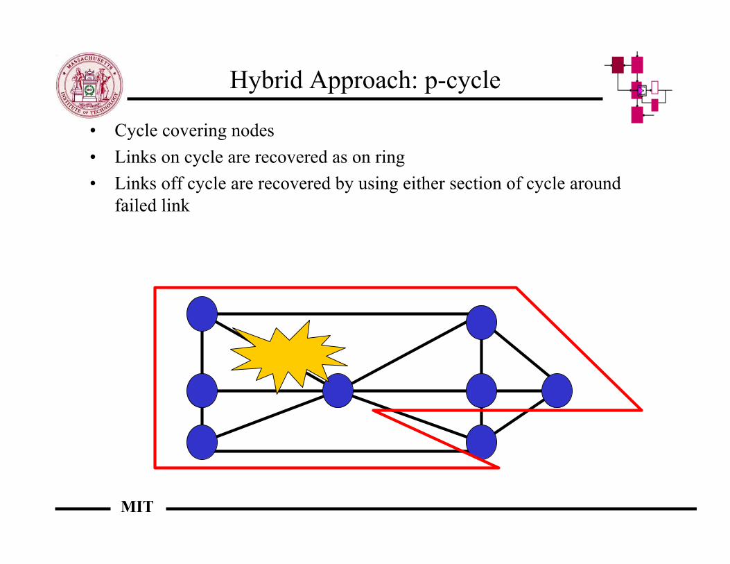
Hybrid Approach: p-cycle
• Cycle covering nodes• Links on cycle are recovered as on ring• Links off cycle are recovered by using either section of cycle around
failed link
MIT
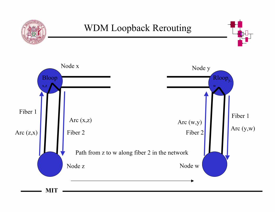
WDM Loopback Rerouting
Node z
Node x Node y
Node w
Fiber 2
Fiber 1
Bloopx,z
Rloopy,w
Fiber 1
Fiber 2Arc (z,x)
Arc (x,z) Arc (w,y)Arc (y,w)
Path from z to w along fiber 2 in the network
MIT
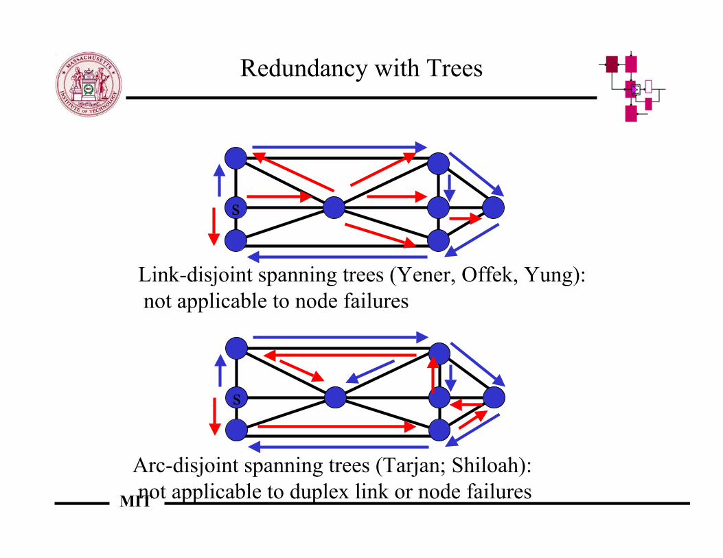
Redundancy with Trees
s
Link-disjoint spanning trees (Yener, Offek, Yung): not applicable to node failures
s
Arc-disjoint spanning trees (Tarjan; Shiloah): not applicable to duplex link or node failures
MIT
Advantages of Trees
• Trees are good for many applications:– multicast and incast applications– hierarchical network management
• The problem of minimum cost multicast tree is NP-complete (Steiner tree problem)
• How to construct 2 trees which allow path rerouting forlink and node failure:– algorithm by Itai and Rodeh based upon a labeling by
Tarjan and Even
MIT
Beyond rerouting
• In rerouting, the source and the destination remain the same,but we change the route between them
• Often rerouting is needed because of congestion rather thanbecause of outright failures and rerouting may not be veryuseful if we have portions of the network around the origin ordestination backed up
• Two new approaches go beyond rerouting:– Change one of the nodes to be in a less congested portion
of the network– Do not reroute, but instead make use of randomness in the
packet losses to code over packet losses
MIT
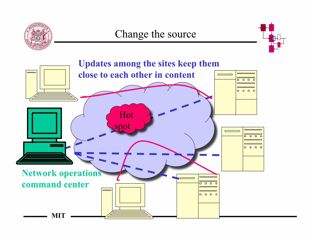
Change the source
• If there is heavy demand at one location, then there will bedelay in that location
• Change to another site that has better characteristics for aparticular user’s location
• Several sites located at the edge of the network can supporta particular request
• A central controller keeps a weathermap of the Internetand assigns the best location for requests – this reduces theload on the individual sites
• Every appears to be request is served as though it wasserved from a single location
MIT
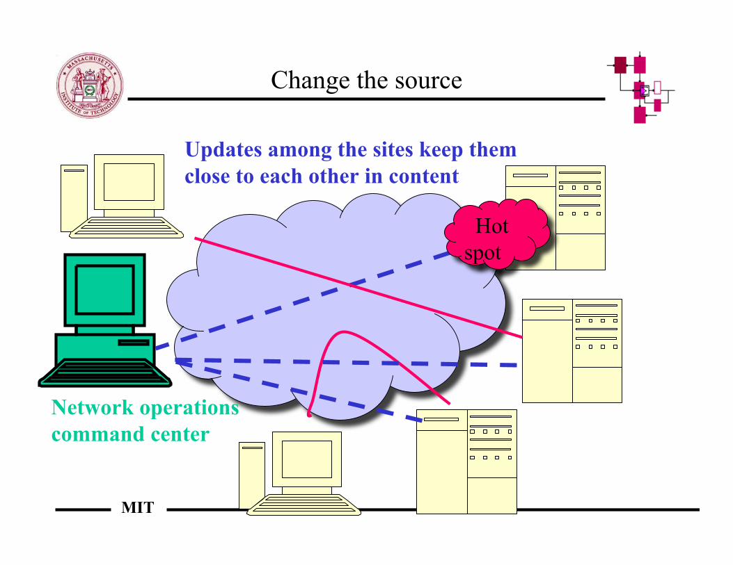
Change the source
Hotspot
Network operationscommand center
Updates among the sites keep them close to each other in content
MIT
Change the source
Hotspot
Network operationscommand center
Updates among the sites keep them close to each other in content
MIT
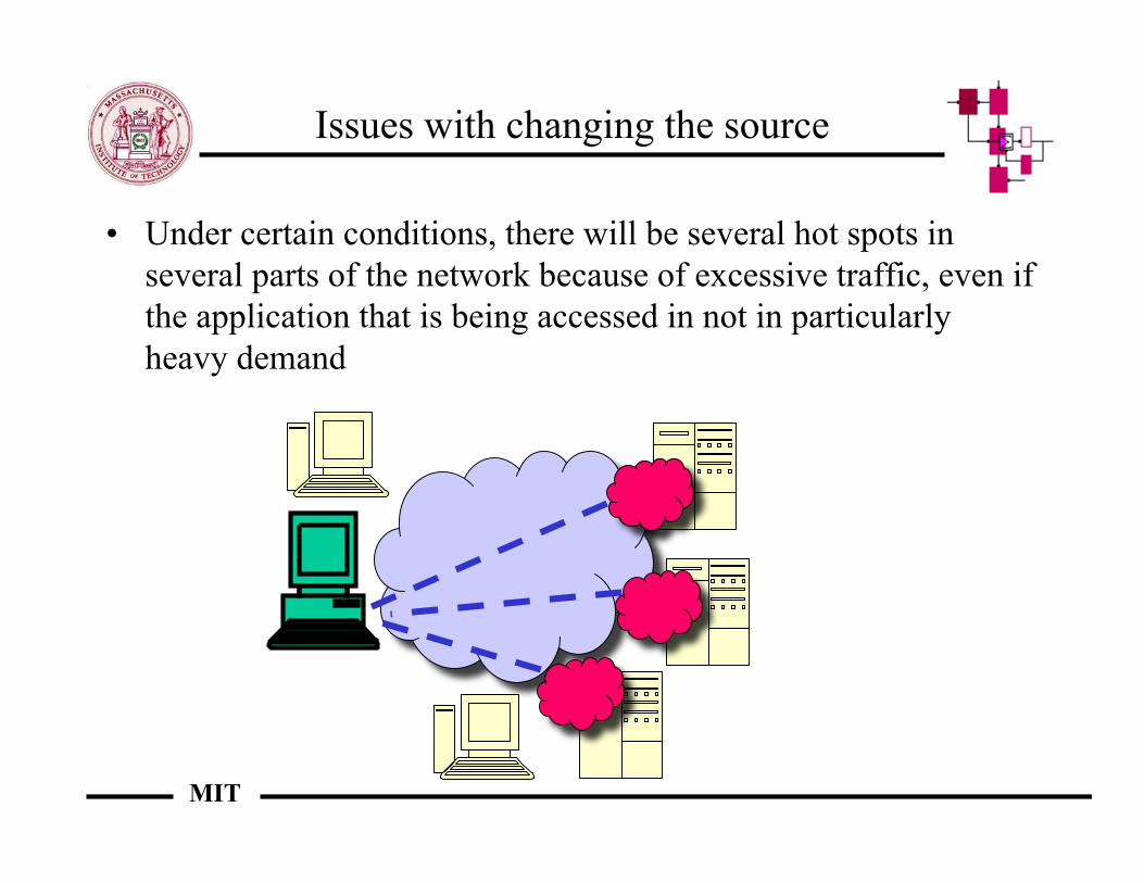
Issues with changing the source
• Under certain conditions, there will be several hot spots inseveral parts of the network because of excessive traffic, even ifthe application that is being accessed in not in particularlyheavy demand
MIT
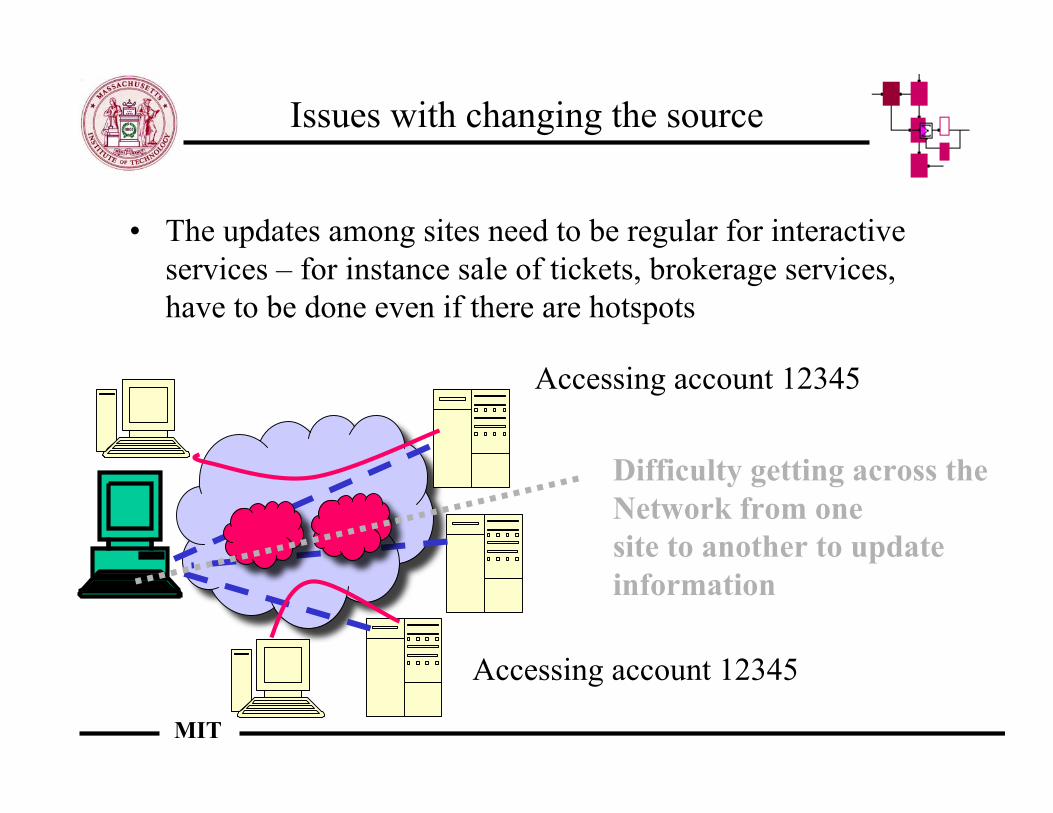
Issues with changing the source
• The updates among sites need to be regular for interactiveservices – for instance sale of tickets, brokerage services,have to be done even if there are hotspots
Difficulty getting across the Network from one site to another to updateinformation
Accessing account 12345
Accessing account 12345
MIT
Coding across the network
• Routing diversity to average out the loss of packets overthe network
• Access several mirror sites rather than single one• The data is then coded across packets in order to withstand
the loss of packets without incurring the loss of all packets• Rather than select the “best” route, we want routes to be
diverse enough that congestion in one location will notbring down a whole stream
• This may be done with traditional Reed-Solomon erasurecodes or with Tornado codes
MIT
Tornado codes
• Use a computationally inexpensive forward erasure-correction code• For every k packets, you create parity and stop after receiving any
distinct k out of (k+l) packets to reconstruct the original data.• Packets are scheduled to minimize the number of duplicate packets
received before getting k distinct ones• Encoding/decoding time is O((l+k)P) for a P-sized packet• For other codes such as Reed-Solomon, typically O(lkP)• See A Digital Fountain Approach to Reliable Distribution of Bulk
Data by John Byers, Michael Luby, Michael Mitzenmacher,Ashutosh Rege
MIT
The digital fountain approach
• Idea: have users tune in whenever they want, and receive dataaccording to the bandwidth that is available at their location inthe network – “fountain” because the data stream is always on
• Create multicast layers: each layer has twice the bandwidth of thelower layer (think of progressively better resolution on images,for instance), except for the first two layers
• If receiver stays at same layer throughout, and packet loss rate islow enough, then receiver can reconstruct source data beforereceiving any duplicate packets : "One-level property"
• Receivers can only subscribe to higher layer after seeingasynchronization point (SP) in their own layer
• The frequency of SPs is inversely proportional to layer BW,
MIT
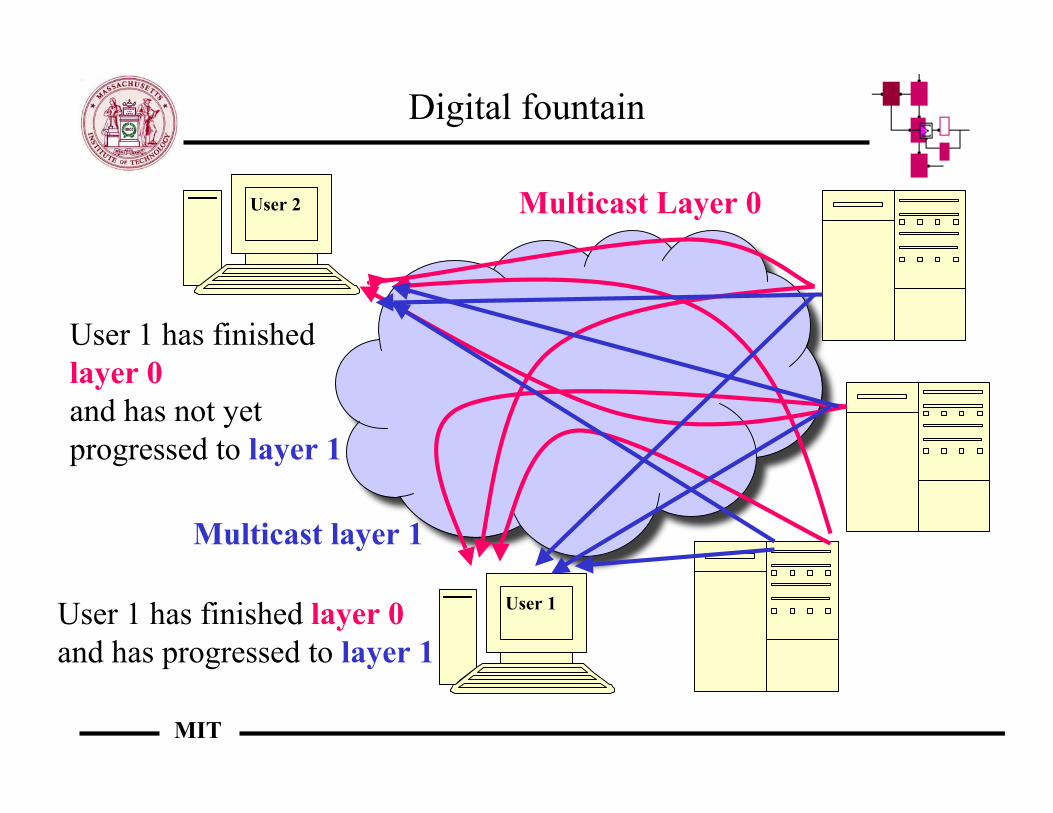
Digital fountain
User 2
User 1
Multicast Layer 0
User 1 has finished layer 0 and has progressed to layer 1
Multicast layer 1
User 1 has finished layer 0 and has not yet progressed to layer 1
MIT
Issues
• The open-loop multicast aspect is attractive – no central nodekeeping track of the network
• The coding seems to be fast• Many questions remain:
– How much delay is induced because of the SPs and how doesthis compare to whatever coding gains may be obtained?
– What is the effect on the higher layer of these delays?– How much network congestion is generated by having the
fountain on at all times and at all points?– How do we do proper interleaving of the data and how do codes
for such interleaving interact with Tornado codes?

MIT
Rerouting as a code
s
t u
b1
b1
b1
b1
w
s . dt,w + s . d u,w = b1
s
t u
b1
w
dt,w + du,w = b1
a. Live path protection b. Link recovery
b1 b1
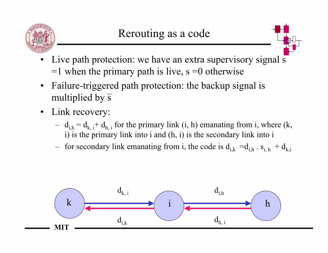
MIT
Rerouting as a code
• Live path protection: we have an extra supervisory signal s=1 when the primary path is live, s =0 otherwise
• Failure-triggered path protection: the backup signal ismultiplied by s
• Link recovery:– di,h = dk, i+ dh, i for the primary link (i, h) emanating from i, where (k,
i) is the primary link into i and (h, i) is the secondary link into i– for secondary link emanating from i, the code is di,k =di,h . si, h + dk,i
di,h
idk, i
k hdi,k dh, i
MIT
Codes and routes
• In effect, every routing and rerouting scheme can be mappedto some type of code, which may involve the presence of anetwork management component
• Thus, removing the restrictions of routing can only improveperformance - can we actively make use of this generality?
MIT
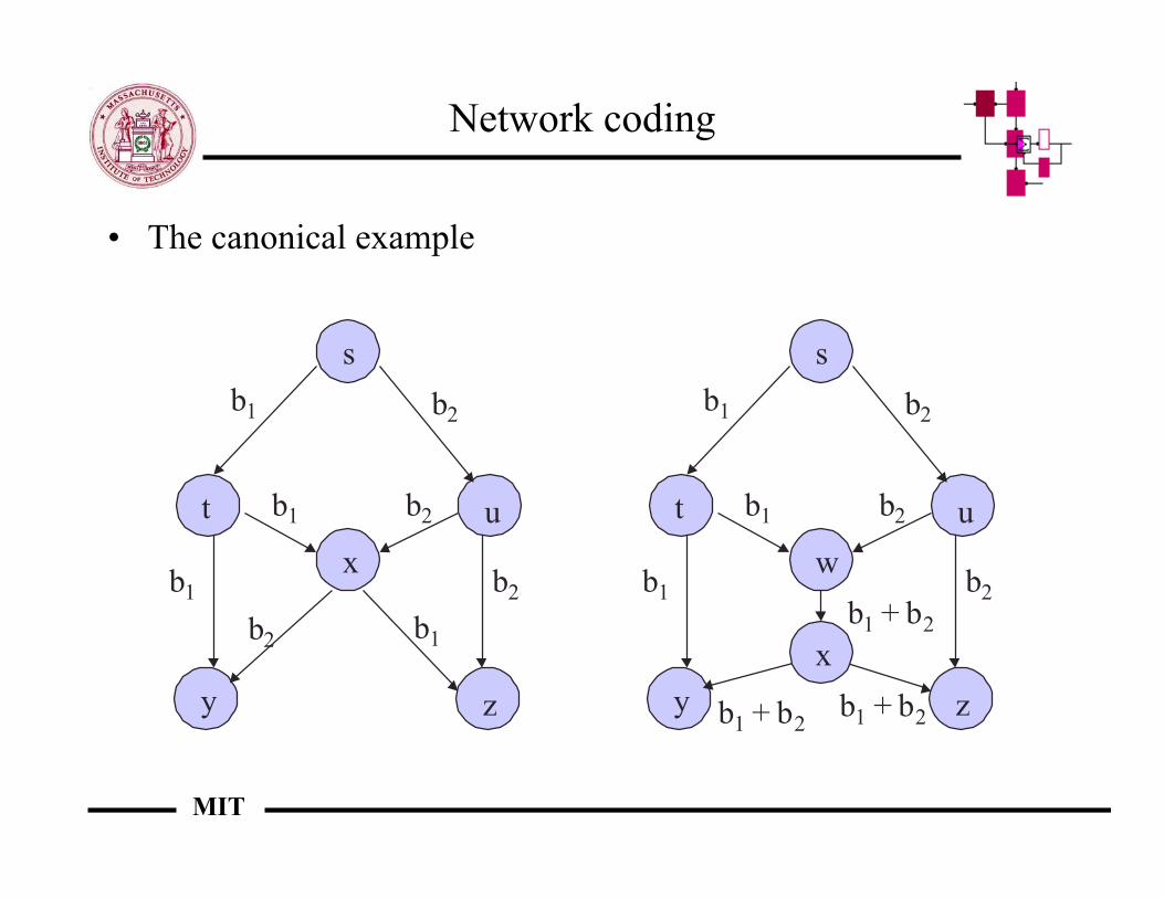
Network coding
• The canonical example
s
t u
y z
x
b1
b1
b1
b1
b2
b2
b2
b2
s
t u
y z
w
b1
b1
b1
b1 + b2
b2
b2
b2
xb1 + b2b1 + b2
MIT
Network coding vs. Coding for networks
• The source-based approaches consider the networks as ineffect channels with ergodic erasures or errors, and code overthem, attempting to reduce excessive redundancy
• The data is expanded, not combined to adapt to topology andcapacity
• Underlying coding for networks, traditional routing problemsremain, which yield the virtual channel over which codingtakes place
• Network coding subsumes all functions of routing - algebraicdata manipulation and forwarding are fused
MIT
Reliable multicast using network codes
• Nodes in networks can randomly select the codes to mixtraffic in the network
• This choice is entirely distributed without any coordinationamong nodes
• There is not need for any node to have information about thenetwork topology, there are no routing tables
• For any general multi-input multicast network, a singlerandomly chosen code can recover from all recoverablefailures - this is not possible with routing (Ho, Koetter,Medard, Karger, Effros, 2003)
• Network recovery in multicast networks can always be donesolely by the receivers, using the knowledge of the compositeeffect of the network (by sending of a canonical basis)
MIT
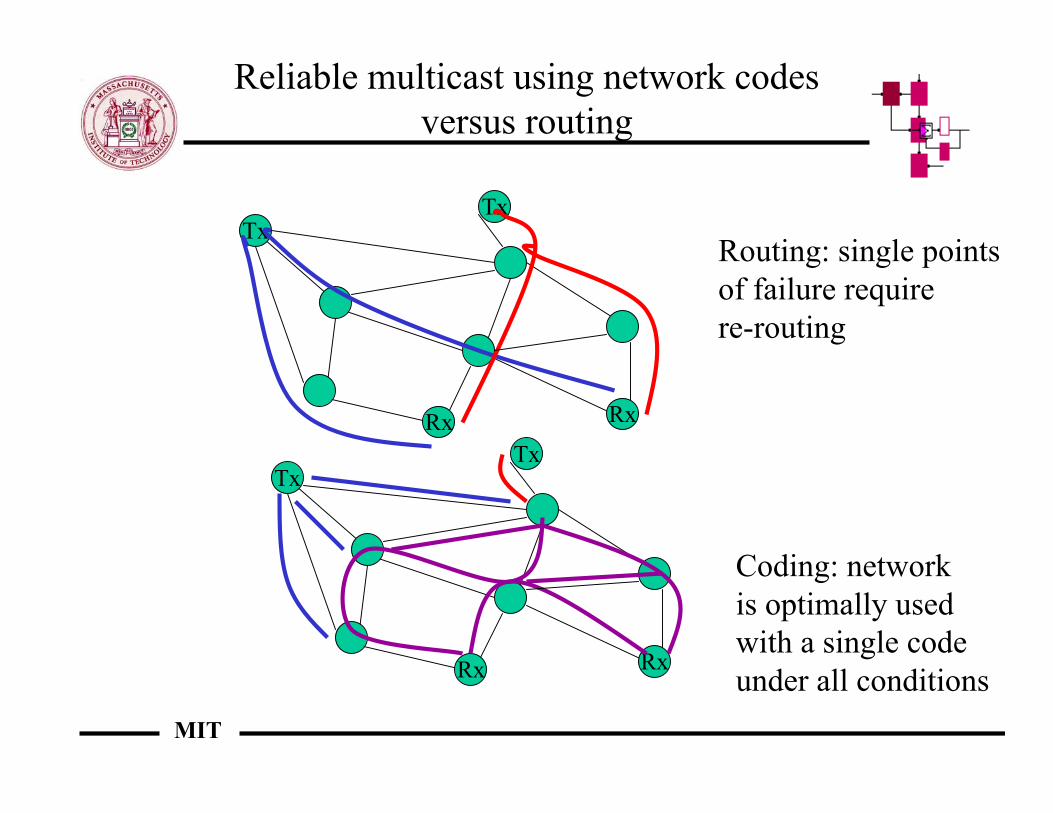
Reliable multicast using network codesversus routing
TxTx
Rx Rx
TxTx
Rx Rx
Routing: single pointsof failure require re-routing
Coding: networkis optimally used with a single codeunder all conditions
Laboratory for Information and Decision SystemsEytan Modiano
Slide 1
LIDS
Flow and congestion control
Eytan Modiano
Laboratory for Information and Decision SystemsEytan Modiano
Slide 2
LIDS
FLOW CONTROL
• Flow control: end-to-end mechanism for regulating traffic between sourceand destination
• Congestion control: Mechanism used by the network to limit congestion
• The two are not really separable, and I will refer to both as flow control
• In either case, both amount to mechanisms for limiting the amount oftraffic entering the network
– Sometimes the load is more than the network can handle
Laboratory for Information and Decision SystemsEytan Modiano
Slide 3
LIDS
WITHOUT FLOW CONTROL
• When overload occurs– queues build up– packets are discarded– Sources retransmit messages– congestion increases => instability
• Flow control prevents network instability by keeping packetswaiting outside the network rather than in queues inside thenetwork
– Avoids wasting network resources– Prevent “disasters”
Laboratory for Information and Decision SystemsEytan Modiano
Slide 4
LIDS
OBJECTIVES OF FLOW CONTROL
• Maximize network throughput
• Reduce network delays
• Maintain quality-of-service parameters– Fairness, delay, etc..
• Tradeoff between fairness, delay, throughput…
Laboratory for Information and Decision SystemsEytan Modiano
Slide 5
LIDS
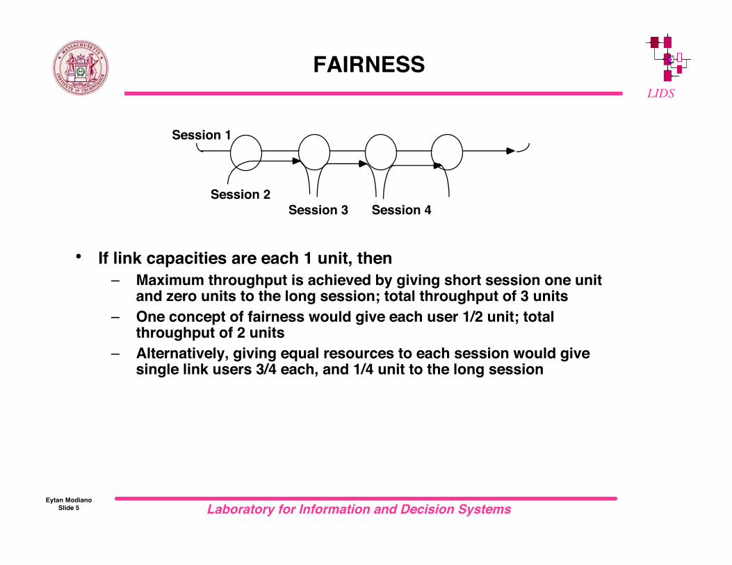
FAIRNESS
• If link capacities are each 1 unit, then– Maximum throughput is achieved by giving short session one unit
and zero units to the long session; total throughput of 3 units– One concept of fairness would give each user 1/2 unit; total
throughput of 2 units– Alternatively, giving equal resources to each session would give
single link users 3/4 each, and 1/4 unit to the long session
Session 1
Session 2
Session 3 Session 4
Laboratory for Information and Decision SystemsEytan Modiano
Slide 6
LIDS
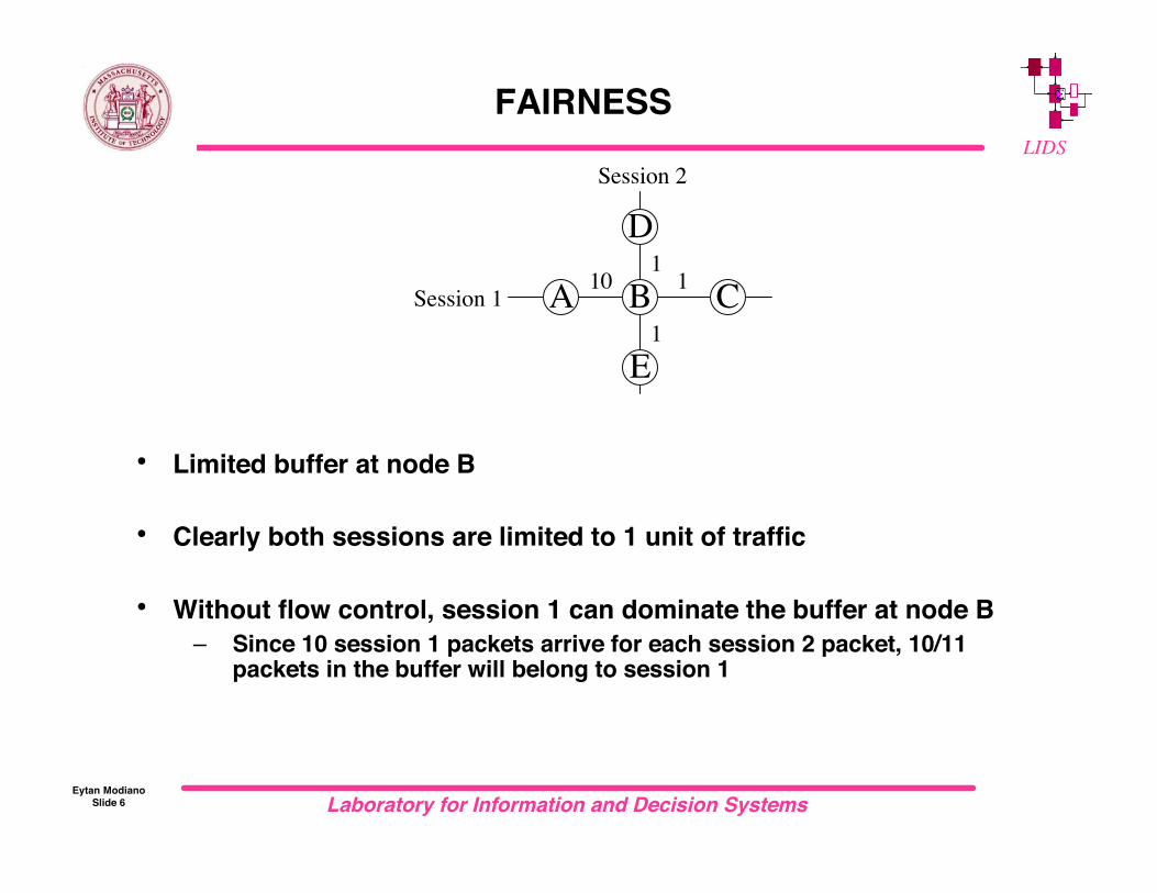
FAIRNESS
• Limited buffer at node B
• Clearly both sessions are limited to 1 unit of traffic
• Without flow control, session 1 can dominate the buffer at node B– Since 10 session 1 packets arrive for each session 2 packet, 10/11
packets in the buffer will belong to session 1
Session 1 CB
D
E
A1
1
110
Session 2
Laboratory for Information and Decision SystemsEytan Modiano
Slide 7
LIDS
A B
A B
C
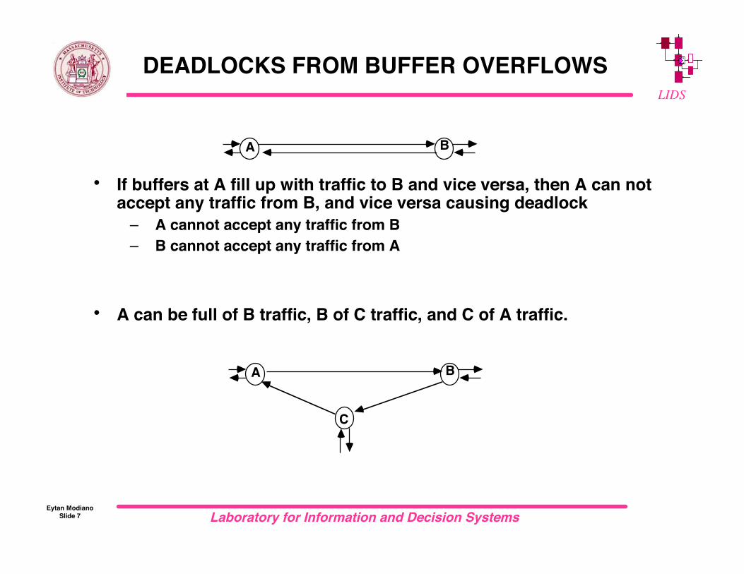
DEADLOCKS FROM BUFFER OVERFLOWS
• If buffers at A fill up with traffic to B and vice versa, then A can notaccept any traffic from B, and vice versa causing deadlock
– A cannot accept any traffic from B– B cannot accept any traffic from A
• A can be full of B traffic, B of C traffic, and C of A traffic.
Laboratory for Information and Decision SystemsEytan Modiano
Slide 8
LIDS
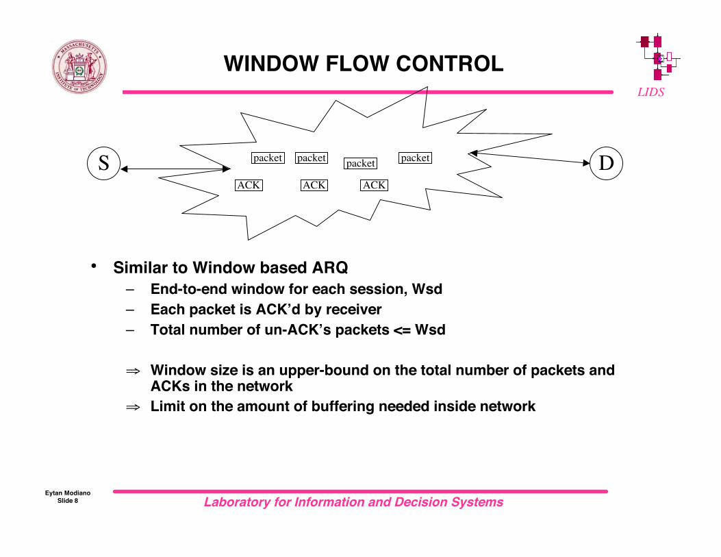
WINDOW FLOW CONTROL
• Similar to Window based ARQ– End-to-end window for each session, Wsd– Each packet is ACK’d by receiver– Total number of un-ACK’s packets <= Wsd
⇒ Window size is an upper-bound on the total number of packets andACKs in the network
⇒ Limit on the amount of buffering needed inside network
S Dpacket packet packet packet
ACK ACK ACK
Laboratory for Information and Decision SystemsEytan Modiano
Slide 9
LIDS
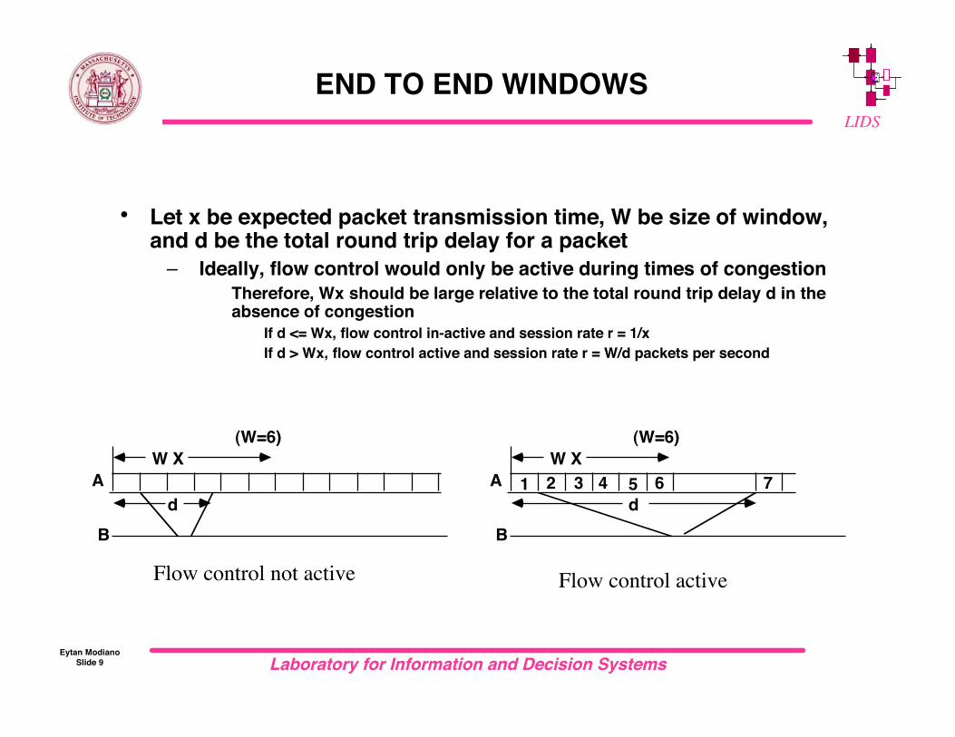
END TO END WINDOWS
• Let x be expected packet transmission time, W be size of window,and d be the total round trip delay for a packet
– Ideally, flow control would only be active during times of congestion Therefore, Wx should be large relative to the total round trip delay d in the
absence of congestion If d <= Wx, flow control in-active and session rate r = 1/x If d > Wx, flow control active and session rate r = W/d packets per second
A
B
(W=6)
W X
d
A
B
(W=6)
W X
d
1 2 3 64 5 7
Flow control not active Flow control active
Laboratory for Information and Decision SystemsEytan Modiano
Slide 10
LIDS
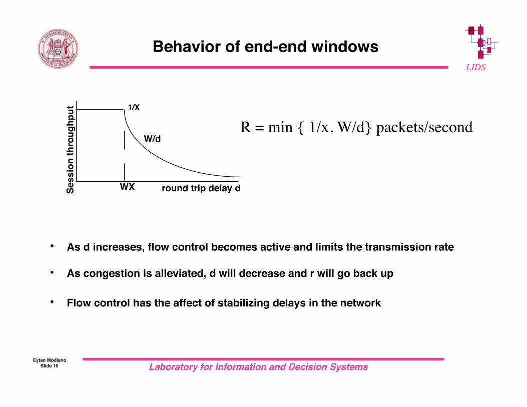
Behavior of end-end windows
• As d increases, flow control becomes active and limits the transmission rate
• As congestion is alleviated, d will decrease and r will go back up
• Flow control has the affect of stabilizing delays in the network
1/X
WX
W/d
round trip delay dSe
ss
ion
th
rou
gh
pu
t
R = min { 1/x, W/d} packets/second
Laboratory for Information and Decision SystemsEytan Modiano
Slide 11
LIDS
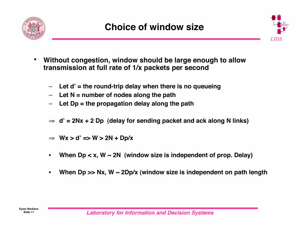
Choice of window size
• Without congestion, window should be large enough to allowtransmission at full rate of 1/x packets per second
– Let d’ = the round-trip delay when there is no queueing– Let N = number of nodes along the path– Let Dp = the propagation delay along the path
⇒ d’ = 2Nx + 2 Dp (delay for sending packet and ack along N links)
⇒ Wx > d’ => W > 2N + Dp/x
• When Dp < x, W ~ 2N (window size is independent of prop. Delay)
• When Dp >> Nx, W ~ 2Dp/x (window size is independent on path length
Laboratory for Information and Decision SystemsEytan Modiano
Slide 12
LIDS
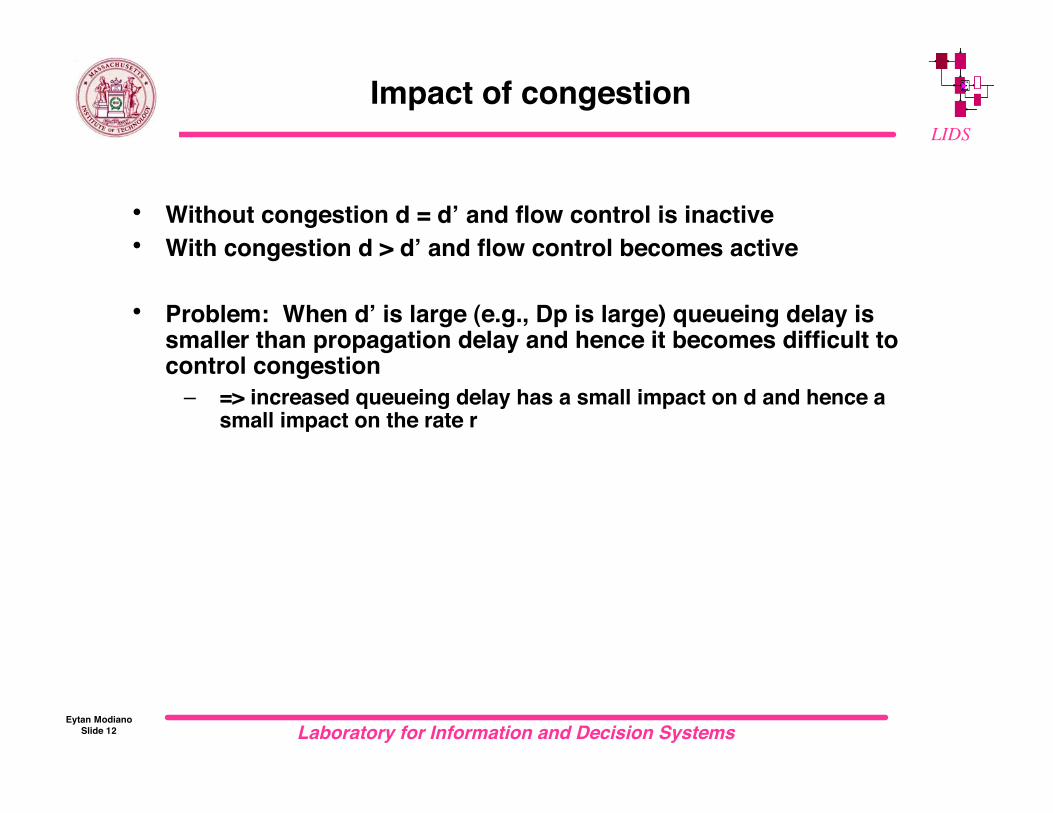
Impact of congestion
• Without congestion d = d’ and flow control is inactive• With congestion d > d’ and flow control becomes active
• Problem: When d’ is large (e.g., Dp is large) queueing delay issmaller than propagation delay and hence it becomes difficult tocontrol congestion
– => increased queueing delay has a small impact on d and hence asmall impact on the rate r
Laboratory for Information and Decision SystemsEytan Modiano
Slide 13
LIDS
PROBLEMS WITH WINDOWS
• Window size must change with congestion level• Difficult to guarantee delays or data rate to a session• For high speed sessions on high speed networks, windows must
be very large– E.g., for 1 Gbps cross country each window must exceed 60Mb– Window flow control becomes in-effective– Large windows require a lot of buffering in the network
• Sessions on long paths with large windows are better treated thanshort path sessions. At a congestion point, large window fills upbuffer and hogs service (unless round robin service used)
Laboratory for Information and Decision SystemsEytan Modiano
Slide 14
LIDS
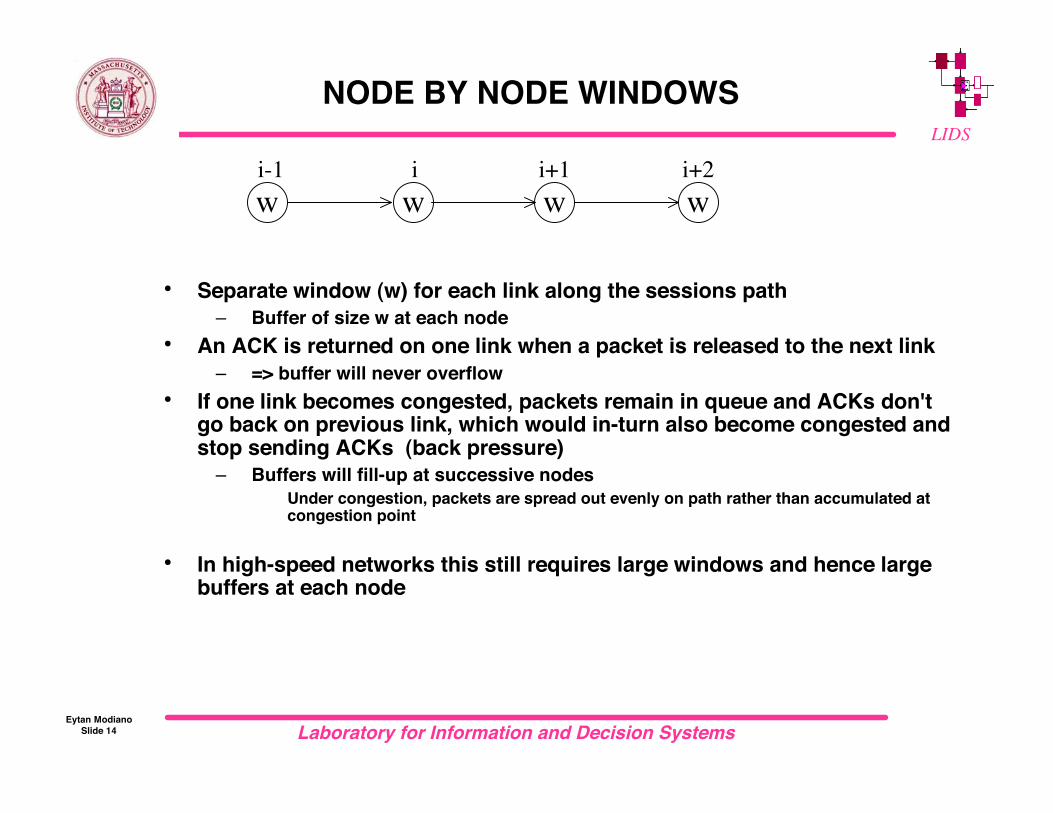
NODE BY NODE WINDOWS
• Separate window (w) for each link along the sessions path– Buffer of size w at each node
• An ACK is returned on one link when a packet is released to the next link– => buffer will never overflow
• If one link becomes congested, packets remain in queue and ACKs don'tgo back on previous link, which would in-turn also become congested andstop sending ACKs (back pressure)
– Buffers will fill-up at successive nodes Under congestion, packets are spread out evenly on path rather than accumulated at
congestion point
• In high-speed networks this still requires large windows and hence largebuffers at each node
w w wwi-1 i i+1 i+2
Laboratory for Information and Decision SystemsEytan Modiano
Slide 15
LIDS
RATE BASED FLOW CONTROL
• Window flow control cannot guarantee rate or delay
• Requires large windows for high (delay * rate) links
• Rate control schemes provide a user a guaranteed rate and some limitedability to exceed that rate
– Strict implementation: for a rate of r packets per second allow exactly onepacket every 1/r seconds
=> TDMA => inefficient for bursty traffic
– Less-strict implementation: Allow W packets every W/r seconds Average rate remains the same but bursts of up to W packets are allowed
Typically implemented using a “leaky bucket” scheme
Laboratory for Information and Decision SystemsEytan Modiano
Slide 16
LIDS
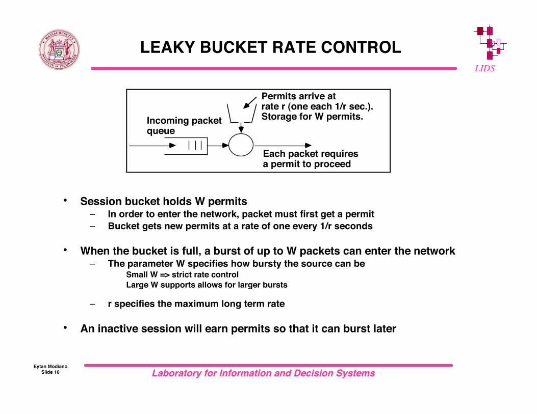
Permits arrive atrate r (one each 1/r sec.).Storage for W permits.Incoming packet
queue
Each packet requiresa permit to proceed
LEAKY BUCKET RATE CONTROL
• Session bucket holds W permits– In order to enter the network, packet must first get a permit– Bucket gets new permits at a rate of one every 1/r seconds
• When the bucket is full, a burst of up to W packets can enter the network– The parameter W specifies how bursty the source can be
Small W => strict rate control Large W supports allows for larger bursts
– r specifies the maximum long term rate
• An inactive session will earn permits so that it can burst later
Laboratory for Information and Decision SystemsEytan Modiano
Slide 17
LIDS
Leaky bucket flow control
• Leaky bucket is a traffic shaping mechanism
• Flow control schemes can adjust the values of W and r inresponse to congestion
– E.g., ATM networks use RM (resource management) cells to tellsources to adjust their rates based on congestion
Laboratory for Information and Decision SystemsEytan Modiano
Slide 18
LIDS
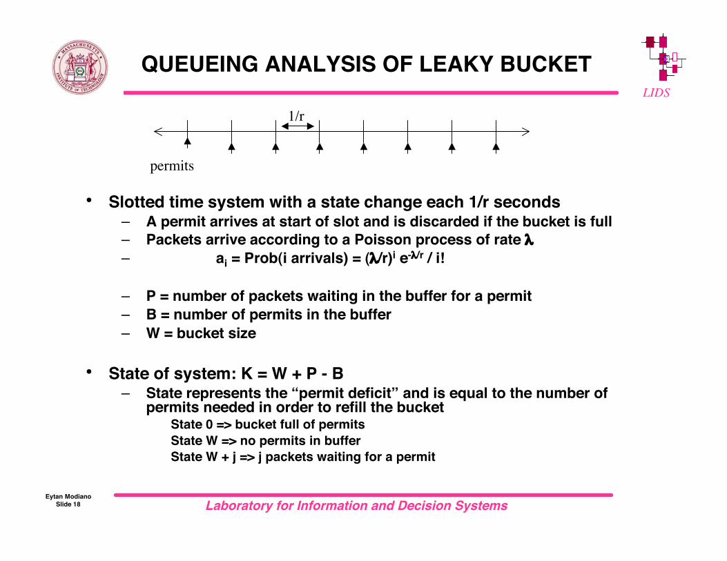
QUEUEING ANALYSIS OF LEAKY BUCKET
• Slotted time system with a state change each 1/r seconds– A permit arrives at start of slot and is discarded if the bucket is full– Packets arrive according to a Poisson process of rate λ– ai = Prob(i arrivals) = (λ/r)i e-λ/r / i!
– P = number of packets waiting in the buffer for a permit– B = number of permits in the buffer– W = bucket size
• State of system: K = W + P - B– State represents the “permit deficit” and is equal to the number of
permits needed in order to refill the bucket State 0 => bucket full of permits State W => no permits in buffer State W + j => j packets waiting for a permit
1/r
permits
Laboratory for Information and Decision SystemsEytan Modiano
Slide 19
LIDS
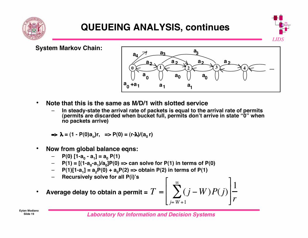
QUEUEING ANALYSIS, continues
System Markov Chain:
• Note that this is the same as M/D/1 with slotted service– In steady-state the arrival rate of packets is equal to the arrival rate of permits
(permits are discarded when bucket full, permits don’t arrive in state “0” whenno packets arrive)
=> λ = (1 - P(0)ao)r, => P(0) = (r-λ)/(a0 r)
• Now from global balance eqns:– P(0) [1-a0 - a1] = a0 P(1)– P(1) = [(1-a0-a1)/a0]P(0) => can solve for P(1) in terms of P(0)– P(1)[1-a1] = a2P(0) + a0P(2) => obtain P(2) in terms of P(1)– Recursively solve for all P(i)’s
• Average delay to obtain a permit =
0 1 2 3 4 ....
a
a
a
a
a
a
aaa
0
1
2
3
0
1
3
2a 2a 2a
0
4
a0+a1
!
T = ( j "W )P( j)j=W +1
#
$%
& ' '
(
) * * 1
r
Laboratory for Information and Decision SystemsEytan Modiano
Slide 20
LIDS
Choosing a value for r
• How do we decide on the rate allocated to a session?
• Approaches
1. Optimal routing and flow control• Tradeoff between delay and throughput
2. Max-Min fairness• Fair allocation of resources
3. Contract based• Rate negotiated for a price (e.g., Guaranteed rate, etc.)

Laboratory for Information and Decision SystemsEytan Modiano
Slide 21
LIDS
Max-Min Fairness
• Treat all sessions as being equal
• Example:
• Sessions S0, S1, S2 share link AB and each gets a fair share of 1/3
• Sessions S3 and S0 share link BC, but since session S0 is limited to 1/3 bylink AB, session S3 can be allocated a rate of 2/3
CA BC = 1 C = 1
S0
S1 S2 S3
Laboratory for Information and Decision SystemsEytan Modiano
Slide 22
LIDS
Max-min notion
• The basic idea behind max-min fairness is to allocate eachsession the maximum possible rate subject to the constraint thatincreasing one session’s rate should not come at the expense ofanother session whose allocated rate is not greater than the givensession whose rate is being increased
– I.e, if increasing a session’s rate comes at the expense of anothersession that already has a lower rate, don’t do it!
• Given a set of session requests P and an associated set of ratesRP, RP is max-min fair if,
– For each session p, rp cannot be increased without decreasing rp’ forsome session p’ for which rp’ <= rp
Laboratory for Information and Decision SystemsEytan Modiano
Slide 23
LIDS
Max-Min fair definition
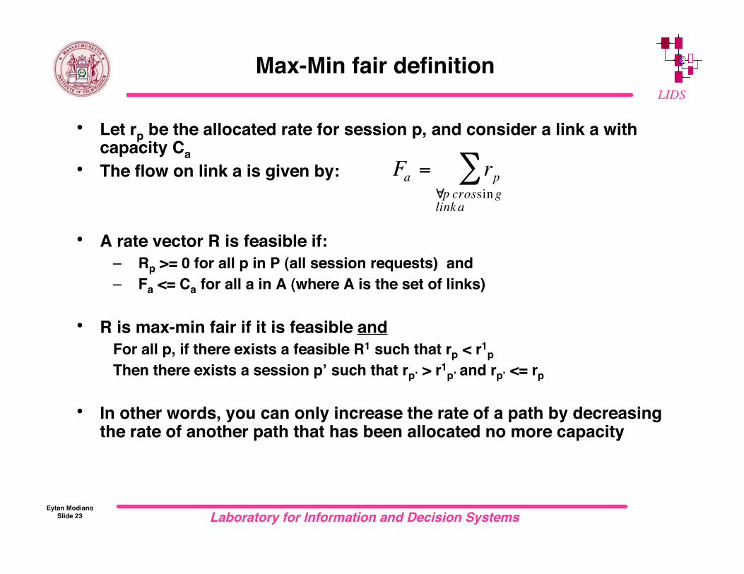
• Let rp be the allocated rate for session p, and consider a link a withcapacity Ca
• The flow on link a is given by:
• A rate vector R is feasible if:– Rp >= 0 for all p in P (all session requests) and– Fa <= Ca for all a in A (where A is the set of links)
• R is max-min fair if it is feasible andFor all p, if there exists a feasible R1 such that rp < r1
pThen there exists a session p’ such that rp’ > r1
p’ and rp’ <= rp
• In other words, you can only increase the rate of a path by decreasingthe rate of another path that has been allocated no more capacity
!
Fa = rp"p crossinglink a
#
Laboratory for Information and Decision SystemsEytan Modiano
Slide 24
LIDS
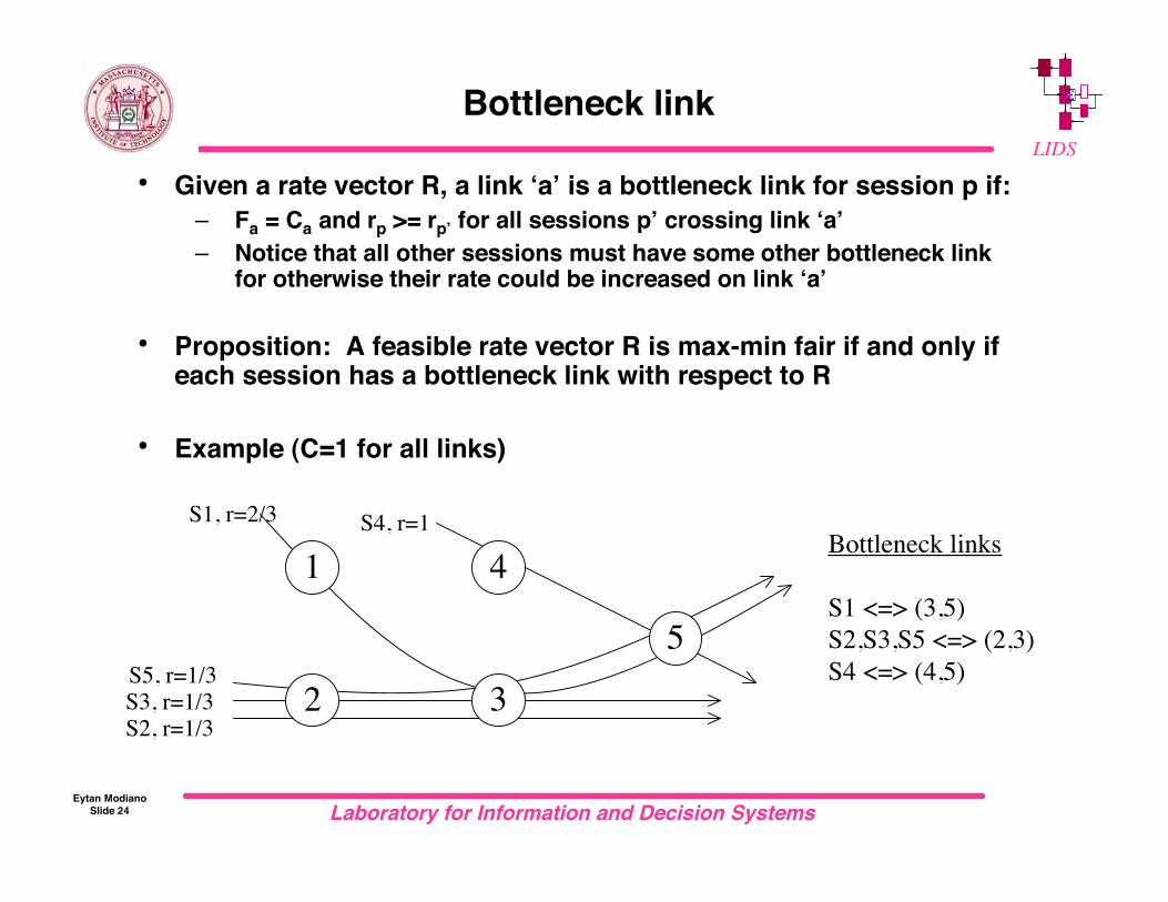
Bottleneck link
• Given a rate vector R, a link ‘a’ is a bottleneck link for session p if:– Fa = Ca and rp >= rp’ for all sessions p’ crossing link ‘a’– Notice that all other sessions must have some other bottleneck link
for otherwise their rate could be increased on link ‘a’
• Proposition: A feasible rate vector R is max-min fair if and only ifeach session has a bottleneck link with respect to R
• Example (C=1 for all links)
S1, r=2/3 S4, r=1
S5, r=1/3S3, r=1/3S2, r=1/3
Bottleneck links
S1 <=> (3,5)S2,S3,S5 <=> (2,3)S4 <=> (4,5)
1 4
5
32
Laboratory for Information and Decision SystemsEytan Modiano
Slide 25
LIDS
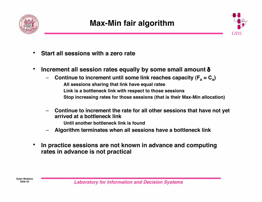
Max-Min fair algorithm
• Start all sessions with a zero rate
• Increment all session rates equally by some small amount δ– Continue to increment until some link reaches capacity (Fa = Ca)
All sessions sharing that link have equal rates Link is a bottleneck link with respect to those sessions Stop increasing rates for those sessions (that is their Max-Min allocation)
– Continue to increment the rate for all other sessions that have not yetarrived at a bottleneck link
Until another bottleneck link is found– Algorithm terminates when all sessions have a bottleneck link
• In practice sessions are not known in advance and computingrates in advance is not practical
Laboratory for Information and Decision SystemsEytan Modiano
Slide 26
LIDS
Generalized processor sharing(AKA fair queueing)
• Serve session in round-robin order– If sessions always have a packet to send they each get an equal
share of the link– If some sessions are idle, the remaining sessions share the capacity
equally
• Processor sharing usually refers to a “fluid” model where sessionrates can be arbitrarily refined
• Generalized processor sharing is a packet based approximationwhere packets are served from each session in a round-robinorder