RoxAnn Measurements and Video based Mussel Mappingfrom Øresund, Denmark: Data Report

Allan Aasbjerg NielsenRasmus LarsenKnut Conradsen

Department of Mathematical ModellingTechnical University of Denmark

Building 321, DK-2800 Lyngby, Denmarke-mail aa,rl,kc@imm.dtu.dk

Internet http://www.imm.dtu.dk

31 August 1996

1 Data

Work is done on two historical datasets from Øresund, the sound between Denmark andSweden.

One data set consists of video based ground truth information on the degree of musselcoverage. This data covers an area of approximately 31 by 19 km

�(the rectangle described

by �������� ��� ����������������������������and �������� ������� � ����! �����������"� ���"����#�

). The original dataset has 30,134 observations. However, some observations a copied in the original dataset. When copies are removed we are left with 29,058 observations. The original valuesin the data have been transformed according to this table

Original value Approximate coverage0 0 %4 15 %3 35 %2 65 %1 90 %

These data are shown in Figure 1.

The other data set consists of RoxAnn measurements (E1,E2) from a smaller area ofapproximately 1.5 by 2.0 km

�. The E1 and E2 values lie between 0 and 2. Also these data

contain copies, and in this case the removal of these reduces the number of observationsfrom 20,478 to 17,292. Figures 2 and 3 show the RoxAnn data.

In the region of overlap between the two data sets ( �$����� � ��� �"������������������������#�and

�����%�&� ����������������������������� ��' ������) we have 842 observations in the mussel coverage data.

Figure 4 shows the mussel coverage in the region covered by RoxAnn data. The positionof the region of overlap between the two data sets is shown with a rectangle in Figure 1.

Figure 5 shows 2-D histograms of E2 and E1 values before (left) and after logarithmtransformations.

2 Spatial Structure

Figure 6 shows the 1-D isotropic semivariogram of the mussel coverage in the region ofoverlap before (left) and after logarithm transformation (before taking logs 0 % coverageis replaced by 1 % coverage). The lag distance is 5 m.

Figure 7 shows the 2-D semivariogram of the mussel coverage in the region of overlap be-fore (left) and after logarithm transformation. The lag distance in both x- and y-directionsis 50 m.

2

Figure 1. Mussel coverage

3

Figure 2. RoxAnn, E1

Figure 3. RoxAnn, E2

4

Figure 4. Mussel coverage in RoxAnn data region

Figure 5. 2-D histograms of (E2,E1) (left) and ln(E2,E1)

5

0

100

200

300

400

500

600

700

0 50 100 150 200 250

Isotropic semivariogram for mussel coverage

0

0.5

1

1.5

2

2.5

3

3.5

0 50 100 150 200 250

Isotropic semivariogram for mussel coverage, ln

Figure 6. 1-D semivariograms of mussel coverage before (left) and after taking logarithms

Figure 7. 2-D semivariograms of mussel coverage before (left) and after taking loga-rithms, 21 ( 21 50 ( 50 m

�pixels

Figure 8 shows 1-D isotropic indicator semivariograms of the mussel coverage in theregion of overlap. The lag distance is 5 m.

Figures 9 and 10 shows 2-D semivariograms of the mussel coverage in the region ofoverlap. In Figure 9 individual stretching is used, In Figure 10 a common stretch is used.The lag distance in both x- and y-directions is 50 m.

Figures 11 and 12 show 1-D isotropic semivariograms of E1 and E2 before (left) and afterlogarithm transformation. The lag distance is 5 m.

Figures 13 and 14 show 2-D semivariograms of E1 and E2 before (left) and after logarithmtransformation. The lag distance in both x- and y-directions is 50 m.

The following table shows parameters for double spheric semivariogram models for theln-transformed variables. The models are based on sample semivariograms with lag val-ues up to 500 m.

Short Range Long Range Nugget Low Sill High Sill[m] [m] [unit

�] [unit

�] [unit

�]

E1 8.882 539.5 0.03419 0.04243 0.08920E2 18.95 6.896 10 )+* 0.02429 0.01844 4.152 10 ,Mussel 7.562 10780 0.000 2.545 10.88

6

0

0.05

0.1

0.15

0.2

0.25

0.3

0 50 100 150 200 250

Isotropic indicator semivariogram for mussel coverage, 1%

0

0.05

0.1

0.15

0.2

0.25

0.3

0 50 100 150 200 250

Isotropic indicator semivariogram for mussel coverage, 25%

0

0.05

0.1

0.15

0.2

0.25

0.3

0 50 100 150 200 250

Isotropic indicator semivariogram for mussel coverage, 50%

0

0.05

0.1

0.15

0.2

0.25

0.3

0 50 100 150 200 250

Isotropic indicator semivariogram for mussel coverage, 75%

Figure 8. 1-D indicator semivariograms of mussel coverage, 1% cutoff (top-left), 25%cutoff (top-right), 50% cutoff (bottom-left), and 75% cutoff (bottom-right)

Figure 9. 2-D indicator semivariograms of mussel coverage, 1% cutoff (top-left), 25%cutoff (top-right), 50% cutoff (bottom-left), and 75% cutoff (bottom-right); 21 ( 21 50 ( 50m�

pixels, individual streching

7

Figure 10. 2-D indicator semivariograms of mussel coverage, 1% cutoff (top-left), 25%cutoff (top-right), 50% cutoff (bottom-left), and 75% cutoff (bottom-right); 21 ( 21 50 ( 50m�

pixels, common streching

0

0.001

0.002

0.003

0.004

0.005

0.006

0.007

0.008

0 50 100 150 200 250

Isotropic semivariogram for E1

0

0.02

0.04

0.06

0.08

0.1

0.12

0.14

0 50 100 150 200 250

Isotropic semivariogram for ln(E1)

Figure 11. 1-D semivariograms of E1 (left) and ln(E1)

0

0.005

0.01

0.015

0.02

0.025

0 50 100 150 200 250

Isotropic semivariogram for E2

0

0.01

0.02

0.03

0.04

0.05

0.06

0 50 100 150 200 250

Isotropic semivariogram for ln(E2)

Figure 12. 1-D semivariograms of E2 (left) and ln(E2)

8

Figure 13. 2-D semivariograms of E1 (left) and ln(E1), 31 ( 41 50 ( 50 m�

pixels

Figure 14. 2-D semivariograms of E2 (left) and ln(E2), 31 ( 41 50 ( 50 m�

pixels

All subsequent work is done on logarithms of both RoxAnn and mussel coveragedata.

3 Interpolation

A 10 meter grid is used for all interpolation schemes applied.

3.1 Weighted Means

Figure 15 shows interpolation of the mussel coverage, E1 and E2 by means of inversedistance weighting. The search radius is 1000 m and a maximum of 50 nearest neighboursare used.

3.2 Kriging

Kriged versions of the mussel coverage, E1 and E2 are shown in Figure 16. The semi-variogram models used are the ones listed above. The search radius is 1000 m and a

9

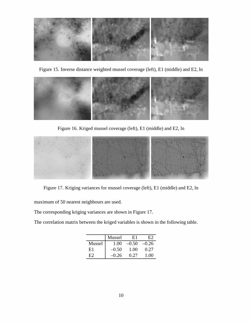
Figure 15. Inverse distance weighted mussel coverage (left), E1 (middle) and E2, ln

Figure 16. Kriged mussel coverage (left), E1 (middle) and E2, ln

Figure 17. Kriging variances for mussel coverage (left), E1 (middle) and E2, ln

maximum of 50 nearest neighbours are used.

The corresponding kriging variances are shown in Figure 17.

The correlation matrix between the kriged variables is shown in the following table.

Mussel E1 E2Mussel 1.00 –0.50 –0.26E1 –0.50 1.00 0.27E2 –0.26 0.27 1.00

10

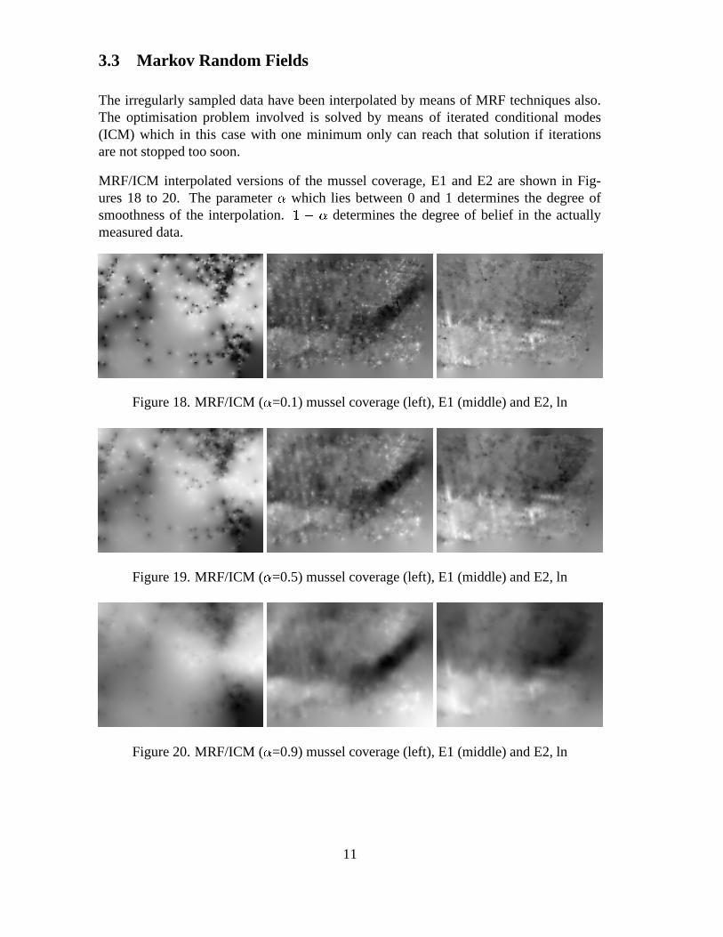
3.3 Markov Random Fields

The irregularly sampled data have been interpolated by means of MRF techniques also.The optimisation problem involved is solved by means of iterated conditional modes(ICM) which in this case with one minimum only can reach that solution if iterationsare not stopped too soon.

MRF/ICM interpolated versions of the mussel coverage, E1 and E2 are shown in Fig-ures 18 to 20. The parameter - which lies between 0 and 1 determines the degree ofsmoothness of the interpolation.

�/. - determines the degree of belief in the actuallymeasured data.

Figure 18. MRF/ICM ( - =0.1) mussel coverage (left), E1 (middle) and E2, ln

Figure 19. MRF/ICM ( - =0.5) mussel coverage (left), E1 (middle) and E2, ln

Figure 20. MRF/ICM ( - =0.9) mussel coverage (left), E1 (middle) and E2, ln

11

Figure 21. Tophat transformations of MRF/ICM ( - =0.9) mussel coverage

4 Patchiness

As a first attempt to visualise patchiness in the mussel coverage a white tophat transforma-tion is applied to the MRF/ICM ( -10 ��23�

) interpolated image. The (negated) results areshown for ever increasing structural elements in Figure 21. The basic structural elementis a 3 ( 3 box.

5 Prediction of Mussel Coverage

As an example of prediction of mussel coverage from RoxAnn data a regression analysisbased on the above kriged version of data is performed. This table summarises the results

12

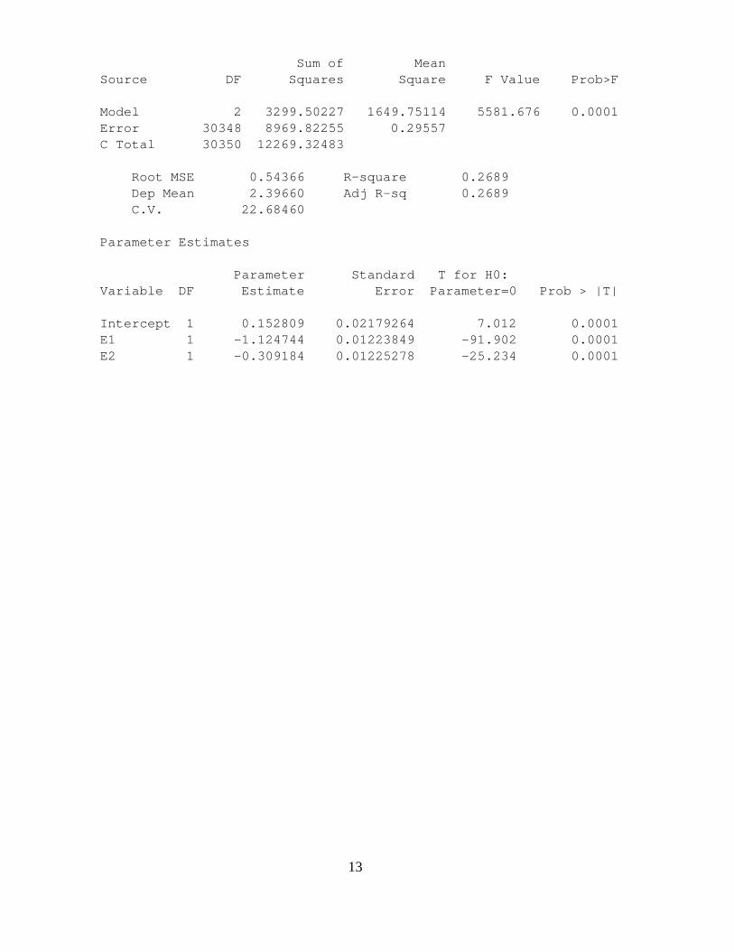
Sum of MeanSource DF Squares Square F Value Prob>F

Model 2 3299.50227 1649.75114 5581.676 0.0001Error 30348 8969.82255 0.29557C Total 30350 12269.32483

Root MSE 0.54366 R-square 0.2689Dep Mean 2.39660 Adj R-sq 0.2689C.V. 22.68460

Parameter Estimates

Parameter Standard T for H0:Variable DF Estimate Error Parameter=0 Prob > |T|

Intercept 1 0.152809 0.02179264 7.012 0.0001E1 1 -1.124744 0.01223849 -91.902 0.0001E2 1 -0.309184 0.01225278 -25.234 0.0001

13

This colour plate shows the the results from the different interpolation techniques as RGBplots. Mussel coverage is shown in red, E1 in green and E2 in blue (after taking loga-rithms). All left plots are scaled linearly between minimum and maximum. All middleplots are scaled linearly between mean value minus three standard deviations and meanvalue plus three standard deviations. All right plots are histogram equalised.

Figure 22. Inverse distance weighted mussel coverage, E1 and E2 as RGB, ln

Figure 23. Kriged mussel coverage, E1 and E2 as RGB, ln

Figure 24. MRF/ICM ( - =0.5) mussel coverage, E1 and E2 as RGB, ln