1

RPR Fairness AlgorithmsNarcıs Puig Camara

puig.camara@gmail.com

Abstract—Resilient Packet Ring (RPR) access method needsfairness algorithms to ensure all stations can transmit without be-ing starved by the ones upstream. This paper tries to summarizethe two standard fairness algorithms and the different proposalsto improve their performance. The RIAS fairness definition isseen. The proposals DVSR, VQ, and Enhanced AM (which tryto get the RIAS solution in a better way than the standard one)are commented. Also the non-RIAS proposals Equal Opportunityfairness and Weighted fairness are exposed.

Index Terms—RPR fairness, Virtual Queuing, DVSR, EqualOpportunity fairness, Enhanced AM, Weighted Fairness.

I. INTRODUCTION

Resilient Packet Ring [1], or RPR, is standardized as IEEE802.17 (June 2004). This standard defines a packet accessprotocol addressed to fit in high rate metropolitan and widearea optical networks which are configured in a ring topology.

The optical ring consists of bidirectional point to pointlinks, which results in a double-ringlet topology. This allowsresilience, which is supposed to provide SONET/SDHprotection features (50ms of maximum recovery time) ina packet based transmission while being physical layerindependent.

In the normal case, only one of the rings is used to transmituser traffic. The other one is a backup ring to make thesystem capable of reaching any point even in case of one linkfailure.

RPR improves SONET/SDH bandwidth allocation, whichis dynamic instead of being static. It also provides auto-restoration and fairness, which the dynamic bandwidthallocation competitor Gigabite Ethernet fails to.

In section II the basic concepts of RPR such as the trafficcategories defined and their priorities are explained. SectionIII states the need of a fairness algorithm. In section IV theRIAS fairness definition is seen and in section V the two RPRstandard fairness algorithms are exposed. In the followingsections, DVSR, Virtual Queuing, Enhanced AggressiveMode, Equal Opportunity and Weighted fairness algorithmsare summarized. Finally, some conclusions and personalopinion are given.

II. RPR BASIC CONCEPTS

The two ringlets are called ringlet 0 and ringlet 1. Only oneof them is used for user traffic when in a normal situation.When a station wants to send a packet, it inserts the data into

Figure 1. RPR network and spatial reuse schema. Source: [2].

the proper ringlet. When the frame reaches the next station,it’s removed from the ringlet if the destination direction isrecognised to be part of the network of that node (outside ofthe ring), or it’s forwarded to the next node if it isn’t. Thisprocess can be done either in a store-and-forward mode orin a cut-through mode – start forwarding the packet whenit hasn’t been completely received yet. To avoid a frame toinfinitely go through the ring, each frame contains a finiteTTL field.

It’s important to note that when a station routes a frameto outside of the ring, it isn’t forwarded inside the ringanymore to allow spatial reuse. That’s freeing the bandwidthof this packet in the rest of the ring where it hasn’t to betransmitted. This allows, as a simple example, simultaneouscommunication between 4 stations (two by two) with all thecapacity available for each group of them if both paths don’tshare any link (as shown in Figure 1, the two flows 1 → i,i+ 1→ n).

A. Access method and traffic categories

As RPR is designed for ring networks, the traffic has tofollow the only path, node over node, until it reaches itsdestination. So, two kinds of traffic can be distinguished ineach node depending on its input.

On the one hand, the node receives traffic from the previousnode in the ring, which can be addressed to this node andwill be taken out of the ring, or can follow the ring. If the

2

Figure 2. Node structure to combine add and transit traffic. Source: [3].

second case occurs, it’s stored into the transit queue untilit can be transmitted to the next node. This is called transittraffic. On the other hand, the traffic input can be the ownnode. In this case, it’s stored in the add queue and willcompete with the transit traffic for being allocated into thelink. The basic behaviour of RPR states that there’s only anadd traffic packet inserted in the ring if the transit queue isempty. A schema of this structure is shown in Figure 2.

The design explained just above doesn’t contain any consid-eration about priorities and it should be improved. That’s whyRPR, a part of his basic behaviour, also defines three classesof traffic. Here are the three classes with its own particularitiesand the subclasses defined for them:

• Class A: low-latency, low-jitter.– A0: reserved bandwidth, only used by the station who

applied for it.– A1: reclaimable bandwidth, if it’s not used, can be

temporally reallocated to other traffic.• Class B: predictable latency, low-jitter.

– B-CIR: committed information rate, also reclaimablebandwidth

– B-EIR: excess information rate. <FE>.• Class C: best effort traffic. <FE>.

The classes labelled with < FE > are called FairnessEligible traffic, which means that they can be controlled bythe fairness algorithms shown later in this paper. It’s alsoimportant to note that the A1 and B-CIR reservations are calledreclaimable bandwidth, so when they are not used FE trafficcan be allocated using these resources.

The reservation of the A0 traffic is done by broadcastover the full ring. After having received all the reservationsfrom all the stations, each of them calculates the quantity ofbandwidth to be permanently allocated for A0 traffic, andthen they know the remaining capacity for reclaimable orFair Eligible traffic.

Linked to the classes of traffic, there are several trafficshapers. Each node has one particular traffic shaper foreach of the A0, A1, B-CIR and FE add traffics, whichcontrols they don’t exceed their limitations. There’s also thedownstream shaper, which manages all the traffic except forA0, and verifies it doesn’t go beyond the unreserved rate limit.

Figure 3. Two queue node structure and priority scheduling. Source: [3].

Figure 4. Two queue nodes simulation latency of the three types of traffic.Source: [3].

As a difference between ATM and other systems, no frameis going to be dropped to solve congestion problems. RPRdoesn’t provide the option to mark exceeded traffic as discard-able in case of congestion. So, all packets will arrive (sooneror later) to its destiny except for errors in their transmission.

To allow A traffic achieve its low-latency and low-jitterproperties, transit queues should be almost always empty.That’s why transit traffic has a higher priority than add traffic,B transit traffic also has more priority than C add traffic, andboth add an transit C traffics compete at the same level.

B. Two transit queues

A more sophisticated structure to reach each traffic classfeatures more accurately, consists of equipping each nodewith two transit queues: Primary Transit Queue (PTQ) andSecondary Transit Queue (STQ). Class A traffic will be storedin the PTQ while classes B and C will be redirected to theSTQ. When choosing the packets to transmit over the link,PTQ frames are the first option. If this queue is empty, thereis a chance for class A add traffic.

The next option is class B add traffic and finally, the lastoption is shared between class C add traffic and STQ frames.This hierarchy is shown in Figure 3. Figure 4 shows the latencyin a simulation of a two queue nodes ring network, wherethe extremely constant latency of A traffic stands out, and Btraffic’s latency is predictable compared to the C one’s. Detailsabout the scenario of this simulation can be found in [3].

3

III. RPR FAIRNESS

At the moment, FE traffic has been seen but it’s stillto comment how this Fairness Eligible traffic is managed.Moreover, it hasn’t been clearly explained how the nodeselects between transmitting C class add traffic or STQtransit traffic. These points are kept on control by the fairnessalgorithm, which is now going to be commented and severalalternatives are discussed in the following.

As explained before, each station transmits an add frameonly if the transit queue is empty – in the simplified case. Inthis situation it’s usual that a station becomes starved by theupstream ones (the ones that fill it with transit traffic). So,if a station received a C rate transit traffic, it couldn’t havesent any add traffic. Hence, the fairness algorithm prevents thedownstream station from this situation.

It’s important to clarify that the rates obtained from thefairness algorithm are only valid for the FE traffic. In theseveral studies to improve these algorithms, FE traffic isalways supposed to be the only one transmitted throughthe ring. Other classes of traffic are omitted because of thebandwidth reservation they dispose of.

But first of all, to be able to implement different alternativesfor a fairness algorithm, the concept of fairness has to bedefined. Several definitions can be found but the RPR standardclarifies that the appropriate fairness definition is the RIASone, which will be summarized at section IV.

As notation remarks, let the node origin of the congestedlink be called the head node, while the more upstream nodetransmitting through this link the tail node. The group of activenodes from the head to the tail one transmitting through thecongested link is called congestion domain.

IV. RIAS FAIRNESS DEFINITION

The Ring Ingress Aggregated with Spatial Reuse (RIAS) issuitable for the RPR scenario. It defines two statements toclarify what can be understood as fair.

1) The granularity level is set to ingress-aggregated flows(IA). This is, all the flows originated at the same nodethat transit through the station running the fairnessalgorithm are treated as an only entity, without matteringits destination.

2) Extra bandwidth can be applied by IA flows when it’snot used. This is used to reach a maximum profit of thespatial reuse.

This algorithm can be generalized to obtain weightedfairness, which is later discussed.

Using the following notation,• f(i, j) flows which go from i to j.• Ri,j : candidate RIAS fair rate for f(i, j).• Fn: allocated rate on link n.

R matrix is said to be feasible if

Ri,j > 0 ∀f(i, j)Fn ≤ C ∀link n (1)

It’s easy to understand that the allocated rate on a link can’tbe greater than this link’s capacity, and that any existing flowshould have an assigned fair rate greater than 0.

Then, n is called a bottleneck link with respect to R forf(i, j) crossing n, denoted by Bn(i, j) if these two conditionsare satisfied:

1) Fn = C2) If IA(i) is the only IA at n,

• Ri,j ≥ Ri,j′ .• If isn’t,

IA(i) ≥ IA(i′) ∀i = i′

and inside this IA(i), Ri,j ≥ Ri,j′ .for all flows crossing link n in each case. Then, the RIAS fairproposition is stated as:

Proposition 1 (RIAS fair): R is RIAS fair if it is feasibleand for each f(i, j), Ri,j can’t be incremented while keepingfeasibility without having to reduce Ri′,j′ for any other flowwhich satisfies Ri,j′ ≤ Ri,j or IA(i′) ≤ IA(i) at the commonlink.

The former condition is to introduce intra-station fairness,while the latter to inter-station. No flow can improve its rateby gaining it against other flows with a lower rate. Intra-station does it by considering all flows coming from the samesource station while inter-station just considers the ingress-aggregates. This behaviour is equivalent to the max-min buthere it’s applied to two different granularities.

As a result, each IA flow will have at it’s disposal no lessthan C

N , but only if has enough add traffic to fill it – N isthe number of active nodes at the selected link n.

To summarize, using this idea of fairness, only one fair rateFn has to be imposed by the congested node n to the othernodes contributing to the congestion. The ones that have loweradd traffic rates will only use part of their rate, while the onesexceeding will have to limit their output rate. As node n isn’tclear about the real requested rate of each node, Fn could bedifficult to calculate and could lead to oscillating estimations.

V. RPR STANDARD FAIRNESS ALGORITHMS

The IEEE 802.17 standard defines two fairness algorithms.Both aim to converge to the RIAS fair solution, but they doit in different ways.

A link is considered as congested when its transit queueoccupation reaches a previously configured threshold. Themain idea, then, is to share the bandwidth between thestations interested in it when demand can’t be afforded. Thecongested station will determine a fair rate for the stationstransmitting through it, which will be communicated by afairness message using the backup ringlet. The reason whythis message goes upstream is to reach as soon as possiblethe stations causing the congestion, which usually are theones immediately before the congested one.

The fair rate is calculated (in a different way depending onRPR-AM or RPR-CM) without having to measure each flow

4

Figure 5. Simulation scenario with two state on/off sources (dynamic trafficapproximation). Source: [4].

Figure 6. RPR-CM link utilization in the simulation result. Source: [4].

rate. This fair rate value will be only estimated because there’seven no way to know the exact required rate for each IA in theactual RPR standardization. As not all of the active stationsmight fully use the fair rate, link n capacity might not befilled even with node n’s add traffic. Then, the fair rate wouldbe increased to reach the RIAS result. Note that this wouldproduce some oscillation before reaching the theoretical value.The way of calculating and updating this rate for new moreaccurate ones is the difference between the two standardizedfairness modes.

A. Conservative mode: RPR-CM

The fair rate is initially established as

BW

N

where N is the number of stations transmitting framesthrough the congested link. This rate is applied only to theFE traffic.

Then, it’s sent to the upstream stations contributing to thecongestion and it’s not updated until all the stations haveadopted their new rate. This adoption is detected by measuringthe congestion state. We can see that in a simulation using thescenario of Figure 5 it results in the oscillation shown in Figure6 where 27% of the capacity is lost at the head node. Thisbehaviour is due to the slow convergence of this algorithm.The simulation considers a dynamic traffic produced by twostate sources.

So, some kind of improvement should be done to avoid thisquite high link usage loss.

B. Aggressive mode: RPR-AM

The fair rate estimation is calculated by low-pass filteringthe add rate of the congestion station — an exponentialaveraging filter. This algorithm continuously transmits thenew fresh estimated fair rates, by default every 100µs. When

Figure 7. RPR-AM schema. Source: [2].

Figure 8. RPR-AM fair rate result over time. Source: [4].

the congestion has already been solved, a fair messageindicating no congestion is sent upwards. Then the previouslyfair rate advised nodes will start to rise gradually their addrates and the head node will become congested again. Atthis time, the average will be more accurate to the RIASsolution and slightly greater than the previous one. Figure 7summarises this process and illustrates where bandwidth losshappens.

In case of static traffic —where changes are due only tothe fairness algorithm not to variable rates of the sourcetraffic— when the STQ gets empty, there’s a lack of amessage to tell the upstream nodes that there are not enoughpackets in the STQ to completely fill up the outgoing frames.At this moment, they keep gradually increasing their ratesaccording to the expression in the same schema, while afaster increase process would reach a better bandwidth usage.This possibility is studied at section VIII.

The simulation in the Figure 5 scenario with the samedynamic traffic as before is shown in Figure 8. In this case,a 16% of usage loss is given due to the same oscillation alsopresent here.

VI. DVSR

The Distributed Virtual time Scheduling in Rings (DVSR)[5] fairness algorithm tries to reach the theoretical RIAS resultnot by oscillating around it by using estimations based on theunused capacity of the congested link, but measuring eachIA rate and defining the fair rate as a function of these. Ofcourse, it requires much more computing resources because

5

of the separate measurement of each IA. But, in contrast, itconverges faster than the previously commented algorithms.

Let the congested node be called node n, and rni the rate

of traffic arriving at node n originated at node i, which has tobe forwarded to the next node. The fair rate for node n, Fn

is calculated as:

Fn =

maxi

{rin

}+(C −

∑i r

in

)if∑

i rin ≤ C

C−∑∀rn

i<Fn

rni

I otherwise(2)

where I = ‖{i : rni ≥ Fn}‖.

So, in the first case,∑

i rin ≤ C includes the case i = n,

which is the n add traffic. Then, this sum takes into accountall the traffic to be transmitted through the congested link, andthe inequality means that the link capacity is not exceeded. Inthis case, the fair rate is set as the maximum IA rate plus theleft capacity.

In the second case, the rate to be transmitted by the link(including node n’s add traffic) exceeds the link capacity. Inthe formula there, the sum takes into account only the alreadyfair IA rates. The capacity not used by these fair IA rates isshared between all the unfair rates. This will reduce the fairrate to fit in C.

As seen in eq. (2), the previous Fn is used to calculate thefair rate Fn (in the sum of the fair IA rates). This makes thatthe algorithm being iterative what requires a loop. Moreover, asort operation has to be performed. That’s why the computingrequirements of this algorithm are important. Its complexityrises at O(N log2N) where N is the number of IA flowsactive at n, while RPR-CM and RPR-AM complexity doesn’tdepend on N .

DVSR algorithm is compared to other proposals in sectionVII-C.

VII. VIRTUAL QUEUING ALGORITHM (VQ)

The Virtual Queuing (VQ) algorithm [4] tries to reach theRIAS fair solution converging faster than RPR-AM and RPR-CM modes while being less costly than DVSR.

A. The main idea

Let rni (k) be the rate of traffic arriving at node n originated

at node i, which has to be forwarded to the next nodeduring the control time interval k. Other notation like previoussections might be used by adding (k) to indicate the k controltime interval instance. Then, the rate of traffic arriving to noden is

rn(k) =∑

i

rni (k) =

∑i 6=n

rni (k)︸ ︷︷ ︸≤C

+ rnn(k)︸ ︷︷ ︸≤Fn(k)

≤ C + Fn(k)

The sum ∑i 6=n

rni (k)

has to be lower than C because, in fact, it comes from then − 1 link which has, in principle, the same capacity as link

Figure 9. Virtual Queuing interpretation of an RPR network. Source: [4].

n. The remaining term rnn(k) represents the congested node

n add traffic. If the previous sum is equal but not less thanC, then node n can’t fairly send its own traffic. Of course,n node add traffic should be lower or equal than its own fairrate Fn.

As the traffic that exceeds the C rate is stored in a queuebefore being transmitted, [4] compares each node to a virtualqueue which service rate is C and its arrivals rate is rn(k).Then, the congestion domain results as shown in Figure 9.

B. The VQ algorithm

In this section the algorithm used by VQ to reach the RIASfair solution is exposed and briefly commented. Let’s commentit’s code, which is in Algorithm 1. Let n indicate the congestednode and Fn(k) the fair rate just previously advertised, whichwill be used to calculate Fn(k+1). Some of the values in thealgorithm are:• Ni(k): Traffic received at n from node i.• Ei: Total quantity of traffic originated at i going throughn, according to the last Fn(k).

• ES : Total traffic quantity of rate-limited nodes.• EU : Total traffic quantity of input-limited nodes — this

is, nodes that can’t fill up their fair rate because their addtraffic rate is lower.

• f : coefficient to multiply to Fn(k) to get the updatedvalue.

1: Ni(k)← rni (k) · T

2: Nn(k)← max {rnn · T, local queue size}

3: Ei ← min {Ni, T · Fn(k)} , ∀i4: ES ←

∑i∈S Ei

5: EU ←∑

i∈U Ei

6: if ES 6= 0 && EU < C · T then7: f ← C·T−EU

ES

8: end if9: if EU ≥ C · T then

10: f ← C·TEU+ES

11: end if12: if ES = 0 &&EU < C · T then13: f ← 114: end if15: Fn(k + 1)← min {f · Fn(k), C}

Algorithm 1: VQ fair rate calculation

The aim of line 3 is to avoid having used old data if the nodei wouldn’t have applied Fn(k) yet. So, the minimum of bothpossible rates is stored in Ei. From line 6, this is equivalent

6

Figure 10. DVSR and VQ ATT upper bounds. Source: [4].

to a max min* algorithm but written quite efficiently. If line6 condition is satisfied, f should be greater than 1 to alleviatethe fair rate because all the capacity isn’t been used. Note thatwhat’s done in this case is to share the total amount of trafficthat can be transmitted without the one transmitted by theinput-limited nodes, between the rate-limited ndoes — in factit’s a way to grant input-limited node rates and distribute thesparse bandwidth between the rate-limited ones (which willhave a greater rate).

On the other hand, line 9 results in f ≤ 1, as max minwould also do because input-limited rates already fill up allthe available bandwidth (including n’s add rate). Finally, inthe last case at line 12, the same fair rate is kept becausethere are only input-limited flows and they don’t need the fullbandwidth, this means that the congestion has been controlled.

C. Simulation and comparison

In the paper, it’s stated that the head node of the congestiondomain is the worst hit one. Therefore, the Accumulatedthrottled traffic (ATT) of this head node is considered a rightfigure of merit to characterize how good is the fair behaviour ofeach algorithm. It’s defined as follows, where < ·> representsthe mean value over a time interval and ATT (L) means totake into account the L control intervals K = 1 . . . L.

ATT (L) =∑

k=1...L

(F (k)− r(k)) · T

<ATT > (L) =∑

k=1...L

F (k)− r(k)L

<ATT > % = 100 · <ATT >∑f=1...L r(k)

· L

In regard to the simulation and comparison, despite alsohaving to measure each IA rate, VQ presentation paper boastsabout having lower computational complexity while betterfairness properties and the same convergence speed as DVSR.Figure 10 shows the analytical comparison of ATT at the headnode upper bound between DVSR and VQ, depending on theon-of ratio for the dynamic traffic two-state sources. It showsthat VQ analytically gives better fairness performance thanDVSR. Figure 11 compares this bound to a simulation and theupper bound is correctly greater than the simulation results. It’salso clear that VQ behaviour is better at the ATT simulation.

Figure 11. Analytical bounds and simulation ATT for DVSR and VQ. Source:[4].

Figure 12. Convergence time comparison between RPR-X and VQ overnumber of nodes in the congestion domain. Source: [4].

Figure 12 compares the convergence time between RPR-AM, RPR-CM and VQ depending on the number of nodes inthe congestion domain. As RPR-CM is better for few nodesthan RPR-AM, VQ shows an incredibly better performance atall scales.

Finally, Figure 13 shows the throughput loss depending onthe off-time to on-time ratio of the two-state traffic sources.Here, VQ is also shown as a better alternative.

DVSR isn’t shown at these last pictures because it’s sup-posed to behave similarly to VQ compared to RPR-X algo-rithms. But what the paper doesn’t speak about is how muchcomputational requirements does VQ use compared to DVSRand RPR-X. It’s said to cost less than DVSR but no idea isshown about how significantly less to be implemented to thenodes. How far is it from DVSR and near to RPR-X? It doesn’tseem to provide such an improvement to this point becauseit’s also based in measuring IA rates and an iterative process

Figure 13. Throughput loss comparison between RPR-X and VQ over on-time to off-time ratio of the two-state sources. Source: [4].

7

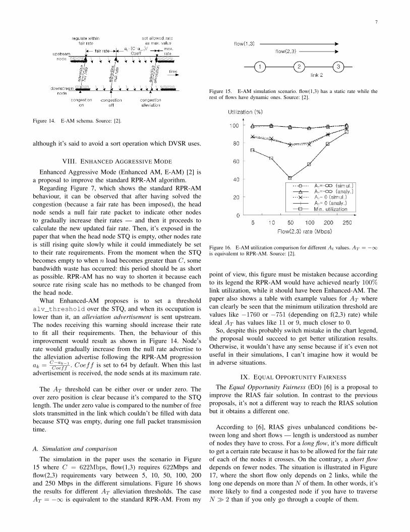
Figure 14. E-AM schema. Source: [2].

although it’s said to avoid a sort operation which DVSR uses.

VIII. ENHANCED AGGRESSIVE MODE

Enhanced Aggressive Mode (Enhanced AM, E-AM) [2] isa proposal to improve the standard RPR-AM algorithm.

Regarding Figure 7, which shows the standard RPR-AMbehaviour, it can be observed that after having solved thecongestion (because a fair rate has been imposed), the headnode sends a null fair rate packet to indicate other nodesto gradually increase their rates — and then it proceeds tocalculate the new updated fair rate. Then, it’s exposed in thepaper that when the head node STQ is empty, other nodes rateis still rising quite slowly while it could immediately be setto their rate requirements. From the moment when the STQbecomes empty to when n load becomes greater than C, somebandwidth waste has occurred: this period should be as shortas possible. RPR-AM has no way to shorten it because eachsource rate rising scale has no methods to be changed fromthe head node.

What Enhanced-AM proposes is to set a thresholdalv_threshold over the STQ, and when its occupation islower than it, an alleviation advertisement is sent upstream.The nodes receiving this warning should increase their rateto fit all their requirements. Then, the behaviour of thisimprovement would result as shown in Figure 14. Node’srate would gradually increase from the null rate advertise tothe alleviation advertise following the RPR-AM progressionak = C−ak−1

Coeff . Coeff is set to 64 by default. When this lastadvertisement is received, the node sends at its maximum rate.

The AT threshold can be either over or under zero. Theover zero position is clear because it’s compared to the STQlength. The under zero value is compared to the number of freeslots transmitted in the link which couldn’t be filled with databecause STQ was empty, during one full packet transmissiontime.

A. Simulation and comparison

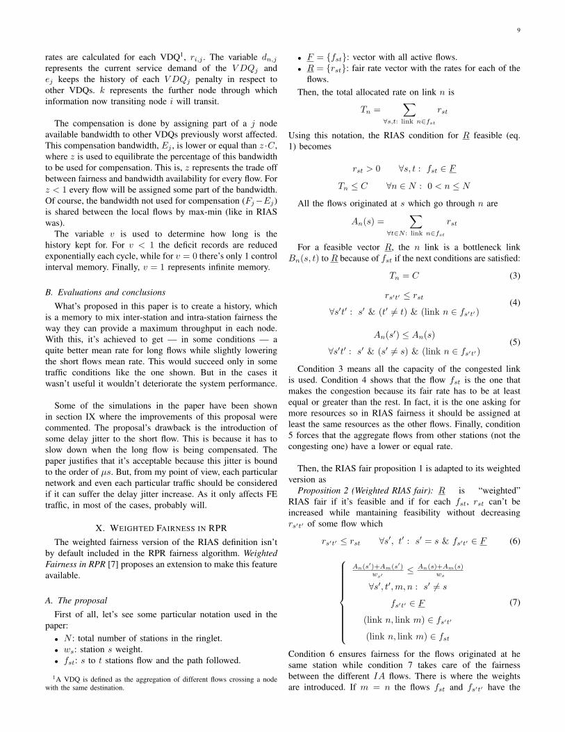
The simulation in the paper uses the scenario in Figure15 where C = 622Mbps, flow(1,3) requires 622Mbps andflow(2,3) requirements vary between 5, 10, 50, 100, 200and 250 Mbps in the different simulations. Figure 16 showsthe results for different AT alleviation thresholds. The caseAT = −∞ is equivalent to the standard RPR-AM. From my

Figure 15. E-AM simulation scenario. flow(1,3) has a static rate while therest of flows have dynamic ones. Source: [2].

Figure 16. E-AM utilization comparison for different At values. AT = −∞is equivalemt to RPR-AM. Source: [2].

point of view, this figure must be mistaken because accordingto its legend the RPR-AM would have achieved nearly 100%link utilization, while it should have been Enhanced-AM. Thepaper also shows a table with example values for AT wherecan clearly be seen that the minimum utilization threshold arevalues like −1760 or −751 (depending on f(2,3) rate) whileideal AT has values like 11 or 9, much closer to 0.

So, despite this probably switch mistake in the chart legend,the proposal would succeed to get better utilization results.Otherwise, it wouldn’t have any sense because if it’s even notuseful in their simulations, I can’t imagine how it would bein adverse situations.

IX. EQUAL OPPORTUNITY FAIRNESS

The Equal Opportunity Fairness (EO) [6] is a proposal toimprove the RIAS fair solution. In contrast to the previousproposals, it’s not a different way to reach the RIAS solutionbut it obtains a different one.

According to [6], RIAS gives unbalanced conditions be-tween long and short flows — length is understood as numberof nodes they have to cross. For a long flow, it’s more difficultto get a certain rate because it has to be allowed for the fair rateof each of the nodes it crosses. On the contrary, a short flowdepends on fewer nodes. The situation is illustrated in Figure17, where the short flow only depends on 2 links, while thelong one depends on more than N of them. In other words, it’smore likely to find a congested node if you have to traverseN � 2 than if you only go through a couple of them.

8

Figure 17. EO long flow and short flow definition. Also EO simulationsscenario. Source: [6].

Figure 18. First link instant rates comparison between RIAS and EO fairnessin Figure 17 scenario and R = 0.5 for short flow. Source: [6].

Still refering to Figure 17, the nodes inside the congestionare modelled as two-state nodes switching between C =100Mbps and 0.2C in periods of T much greater than theconvergence time (to avoid discussing about convergence andkeep the interest in final solutions). The short and long flows,which are the case of study, have both the same demand 0.5Cso that they can completely use the first link equally.

Figure 18 (a) shows the simulation results (for N=7 nodesin the congestion domain) comparing the RIAS model (aand b) and de EO fairness (c and d). As we can see in (b),the short flow is assigned 50% of the full capacity (let R bethe short flow rate requirements, R = 0.5C), while the longflow oscillates depending on the head node congestion. It’smaximum rate (when there’s no congestion at node n) is 0.5C.

What EO fairness tries to improve is this punctual issuein RIAS inter-station fairness. It tries to keep some kind ofhistory of the penalization a flow gets and compensate it whenthe downstream congestion allows it.

In the example, when nodes {2 . . . N − 1} are in high state,there’s no choice for the long flow to reduce its speed underthe fair rate it’s been assigned, while the short flow is freeto transmit its required 0.5C. But, when nodes {2 . . . N − 1}are in low state, RIAS would allow the long flow to share thefirst link bandwidth with the short flow in equal parts: 0.5Cfor each.

What EO fairness would do in that case is to compensatethe previous penalty for the long one and let it transmit asmuch as the N node fair rate permits. Moreover, when thelong flow was limited by the N node fair rate, the short flowwould be capable to send the previously throttled traffic, now

Figure 19. First link average utilization when R = 0.8 for short flow.Comparison between RIAS and EO fairness in Figure 17 scenario.

Figure 20. EO algorithm to find the non-RIAS solution.

faster than 0.5C.The normalized mean rates of the example and R = 0.8

(short flow rate requirements), for the RIAS case are r1,2 =0.650 and r1,7 = 0.333. In the case of EO fairness, they wouldimprove to r1,2 = 0.517 and r1,7 = 0.483 as seen in Figure19.

This behaviour would increase the long flow mean ratewhile slightly decreasing the short flow one, but the first link(1 → 2) total throughput would be kept near 100%. In thisscenario, RIAS results in a 17% throughput loss in link 1→ 2.

A. The proposed algorithm

The concrete proposed algorithm is shown in Figure 20.Let’s see what some of the variables are used for.

After each control interval, the fair rates Fi of thedownstream nodes are received. Then, the EO fair service

9

rates are calculated for each VDQ1, ri,j . The variable dn,j

represents the current service demand of the V DQj andej keeps the history of each V DQj penalty in respect toother VDQs. k represents the further node through whichinformation now transiting node i will transit.

The compensation is done by assigning part of a j nodeavailable bandwidth to other VDQs previously worst affected.This compensation bandwidth, Ej , is lower or equal than z ·C,where z is used to equilibrate the percentage of this bandwidthto be used for compensation. This is, z represents the trade offbetween fairness and bandwidth availability for every flow. Forz < 1 every flow will be assigned some part of the bandwidth.Of course, the bandwidth not used for compensation (Fj−Ej)is shared between the local flows by max-min (like in RIASwas).

The variable v is used to determine how long is thehistory kept for. For v < 1 the deficit records are reducedexponentially each cycle, while for v = 0 there’s only 1 controlinterval memory. Finally, v = 1 represents infinite memory.

B. Evaluations and conclusions

What’s proposed in this paper is to create a history, whichis a memory to mix inter-station and intra-station fairness theway they can provide a maximum throughput in each node.With this, it’s achieved to get — in some conditions — aquite better mean rate for long flows while slightly loweringthe short flows mean rate. This would succeed only in sometraffic conditions like the one shown. But in the cases itwasn’t useful it wouldn’t deteriorate the system performance.

Some of the simulations in the paper have been shownin section IX where the improvements of this proposal werecommented. The proposal’s drawback is the introduction ofsome delay jitter to the short flow. This is because it has toslow down when the long flow is being compensated. Thepaper justifies that it’s acceptable because this jitter is boundto the order of µs. But, from my point of view, each particularnetwork and even each particular traffic should be consideredif it can suffer the delay jitter increase. As it only affects FEtraffic, in most of the cases, probably will.

X. WEIGHTED FAIRNESS IN RPR

The weighted fairness version of the RIAS definition isn’tby default included in the RPR fairness algorithm. WeightedFairness in RPR [7] proposes an extension to make this featureavailable.

A. The proposal

First of all, let’s see some particular notation used in thepaper:• N : total number of stations in the ringlet.• ws: station s weight.• fst: s to t stations flow and the path followed.

1A VDQ is defined as the aggregation of different flows crossing a nodewith the same destination.

• F = {fst}: vector with all active flows.• R = {rst}: fair rate vector with the rates for each of the

flows.Then, the total allocated rate on link n is

Tn =∑

∀s,t: link n∈fst

rst

Using this notation, the RIAS condition for R feasible (eq.1) becomes

rst > 0 ∀s, t : fst ∈ F

Tn ≤ C ∀n ∈ N : 0 < n ≤ N

All the flows originated at s which go through n are

An(s) =∑

∀t∈N : link n∈fst

rst

For a feasible vector R, the n link is a bottleneck linkBn(s, t) to R because of fst if the next conditions are satisfied:

Tn = C (3)

rs′t′ ≤ rst

∀s′t′ : s′ & (t′ 6= t) & (link n ∈ fs′t′)(4)

An(s′) ≤ An(s)

∀s′t′ : s′ & (s′ 6= s) & (link n ∈ fs′t′)(5)

Condition 3 means all the capacity of the congested linkis used. Condition 4 shows that the flow fst is the one thatmakes the congestion because its fair rate has to be at leastequal or greater than the rest. In fact, it is the one asking formore resources so in RIAS fairness it should be assigned atleast the same resources as the other flows. Finally, condition5 forces that the aggregate flows from other stations (not thecongesting one) have a lower or equal rate.

Then, the RIAS fair proposition 1 is adapted to its weightedversion as

Proposition 2 (Weighted RIAS fair): R is “weighted”RIAS fair if it’s feasible and if for each fst, rst can’t beincreased while mantaining feasibility without decreasingrs′t′ of some flow which

rs′t′ ≤ rst ∀s′, t′ : s′ = s & fs′t′ ∈ F (6)

An(s′)+Am(s′)ws′

≤ An(s)+Am(s)ws

∀s′, t′,m, n : s′ 6= s

fs′t′ ∈ F

(link n, link m) ∈ fs′t′

(link n, link m) ∈ fst

(7)

Condition 6 ensures fairness for the flows originated at hesame station while condition 7 takes care of the fairnessbetween the different IA flows. There is where the weightsare introduced. If m = n the flows fst and fs′t′ have the

10

Figure 21. Weighted fairness scenario. Source: [7].

same bottleneck — they are both to blame for the congestionthere. If m 6= n both flows don’t have any common bottleneckbut one goes though the other’s bottleneck.

Note that this proposal requires measuring the rate of eachparticular ingress aggregated flow, operation not performed bythe two standard algorithms and which significantly increasesthe computational complexity of the process.

B. Example scenario

The paper [7] proposes an example scenario where touse weighted fairness. This same scenario is also used forsimulations in section X-C. Figure 21 shows the way thenodes are connected. Node 5 is a video server with a 400Mbpsupload rate (50 TV channels), which is sent to the nodes 6, 7and 8 (video customers). Moreover, node 4 is the gateway tothe internet while nodes 6, 7 and 8 download 300Mbps fromthere (an aggregated of 200 connections of 1.5Mbps per finaluser). The link capacity is C = 600Mbps.

If the RIAS fair solution is applied to this scenario, node 4and node 5 get the same rate (the link 5 → 6 is supposed tobe congested (400Mbps + 300Mbps > C). In this case, only37 of the 50 TV channels could be transmitted.

The weighted RIAS solution would allow assigning ahigher weight to the video traffic so that all the TV channelscould be transmitted. To determine the weight to assign, the400Mbps of video have to be taken into account. Then, fornode 4 should remain 600− 400 = 200. From this result,

w5 =400Mbps200Mbps

= 2

w4 = 1

From my point of view, this scenario is not really typicalbecause what I would do to combine both internet and videotraffic is establish a different class for the video one. If ithad been class A or class B-CIR it wouldn’t have neededsuch weights to ensure its required rate. So, concept of thescenario may be a little bit unrealistic but, of course, the needof weights could be applied to other situations more credible.

C. Simulation results

The results show that the previous scenario doesn’t work asexpected: they get the bandwidth shared 50%-50% betweenthe nodes 4 and 5, despite their different weights. Moreover,there’s a quite big amplitude undesired oscillation. Theproblem is that the highest weighted node selects to transmita packet from the STQ than the add traffic queue too often.That’s why if the nodes 4 and 5 positions are switched, theresults are the ones expected.

To definitively solve this issue, the selection algorithm ofthe RPR has to be modified by inserting the local weightwhen choosing between STQ or add traffic. It’s necessary todivide the add rate or to multiply the forward rate with thelocal weight. This increments the computational requirementsof the algorithm but the paper suggests to assign the weightsas power of 2 because then the new multiplication is just ashift right operation.

This solution works properly and the results are the onesexpected without such a big oscillation.

XI. CONCLUSIONS

There are several proposals to improve the RPR-AMalgorithm which mostly try to address the oscillation and thespeed of convergence. As there are such proposals trying tosolve the same two problems, they can be understood as themain standard fairness algorithms weaknesses.

There’s the trade off between speed of convergence andcomputing requirements. From my point of view, the bestequilibrated one for this seems to be the VQ proposal, but it’sjust an opinion because there aren’t many details about thecomplexity reducement of this proposal against DVSR. Alsothe Enhanced-AM is a nice way to improve the throughputwithout too many changes.

There are also a few algorithms that discuss the possibilityof changing the RIAS solution. The first of them is the EqualOpportunity fairness. It could be a good idea in some casesbut the delay jitter introduced could be a problem. The otherone is the Weighted extension of the RIAS solution, whichin my opinion could be introduced in the standard becauseit hasn’t any important drawback (a part from a probableincrease of computing requirements which isn’t detailed).

Finally, just saying that these are some examples of lots ofimprovements published which were selected to get an ideaabout what are the weak points in RPR fairness algorithmsand different aproaches for solving them.

REFERENCES

[1] IEEE, IEEE Standard 802.17: Resilient Packet Ring,http://www.ieee802.org/17, 2004.

[2] T. J. Kim, “Design of an enhanced fairness algorithm for the IEEE 802.17resilient packet ring,” pp. 1–4, 2005.

11

[3] F. Davik, M. Yilmaz, S. Gjessing, and N. Uzun, “IEEE 802.17 resilientpacket ring tutorial,” Communications Magazine, IEEE, vol. 42, no. 3,pp. 112–118, 2004.

[4] A. Shokrani, S. Khorsandi, I. Lambadaris, and L. Khan, “Virtual queuing:an efficient algorithm for bandwidth management in resilient packetrings,” pp. 982–988 Vol. 2, 2005.

[5] V. Gambiroza, P. Yuan, L. Balzano, Y. Liu, S. Sheafor, and E. Knightly,“Design, analysis, and implementation of DVSR: a fair high-performanceprotocol for packet rings,” IEEE/ACM Transactions on Networking,vol. 12, no. 1, pp. 85–102, 2004.

[6] S. Khorsandi, A. Shokrani, and I. Lambadaris, “Equal opportunity fairnessin resilient packet rings,” pp. 994–1001, 2006.

[7] M. Yilmaz and N. Ansari, “Weighted fairness in resilient packet rings,”pp. 2192–2197, 2007.