rpsea final report - national energy technology … library/research/oil-gas/07121-1901... ·...
TRANSCRIPT

RPSEA
Final Report 07121-1901.FINAL
Subsea Processing Simulator
07121-1901
July 15, 2011
Chris Wolfe Manager, Seals Lab
General Electric Global Research 1 Research Circle
Niskayuna, NY 12309
Subsea Processing Simulator – 07121-1901 Final Report 2
LEGAL NOTICE
This report was prepared by General Electric Global Research as an account of work sponsored by the Research Partnership to Secure Energy for America, RPSEA. Neither RPSEA members of RPSEA, the National Energy Technology Laboratory, the U.S. Department of Energy, nor any person acting on behalf of any of the entities:
a. MAKES ANY WARRANTY OR REPRESENTATION, EXPRESS OR IMPLIED WITH RESPECT TO ACCURACY, COMPLETENESS, OR USEFULNESS OF THE INFORMATION CONTAINED IN THIS DOCUMENT, OR THAT THE USE OF ANY INFORMATION, APPARATUS, METHOD, OR PROCESS DISCLOSED IN THIS DOCUMENT MAY NOT INFRINGE PRIVATELY OWNED RIGHTS, OR
b. ASSUMES ANY LIABILITY WITH RESPECT TO THE USE OF, OR FOR ANY AND ALL
DAMAGES RESULTING FROM THE USE OF, ANY INFORMATION, APPARATUS, METHOD, OR PROCESS DISCLOSED IN THIS DOCUMENT.
THIS IS A FINAL REPORT. THE DATA, CALCULATIONS, INFORMATION, CONCLUSIONS, AND/OR RECOMMENDATIONS REPORTED HEREIN ARE THE PROPERTY OF THE U.S. DEPARTMENT OF ENERGY. REFERENCE TO TRADE NAMES OR SPECIFIC COMMERCIAL PRODUCTS, COMMODITIES, OR SERVICES IN THIS REPORT DOES NOT REPRESENT OR CONSTIITUTE AND ENDORSEMENT, RECOMMENDATION, OR FAVORING BY RPSEA OR ITS CONTRACTORS OF THE SPECIFIC COMMERCIAL PRODUCT, COMMODITY, OR SERVICE.
Subsea Processing Simulator – 07121-1901 Final Report 3
ABSTRACT The RPSEA Simulator is a general purpose process simulator featuring minimal architectural overhead that puts all the functionality in user developed unit models. The underlying goal is to remove all unnecessary impediments to allow the user full modeling license. Hierarchical modeling is enabled by standardized unit model interfaces, arbitrarily expandable data structures, tag-based calls, and an organization that aids, if not enforces, documentation. Pre- and post-processing statistics modules were developed. For validation a flow loop with a three-phase gravity separator was built, and a test matrix was executed with fresh and salt water, model oil and air. The RPSEA Simulator was used to develop a separation simulator, the results of which were compared to test results from an experimental flow loop.

Subsea Processing Simulator – 07121-1901 Final Report 4

Subsea Processing Simulator – 07121-1901 Final Report 5
THIS PAGE INTENTIONALLY LEFT BLANK

Subsea Processing Simulator – 07121-1901 Final Report 6
Subsea Processing Simulator
Final Report
RPSEA Project No. 07121-1901
David Anderson Chris Wolfe Mahadevan Balasubramaniam Luciano Patruno Ryan Qi
July 15, 2011

Subsea Processing Simulator – 07121-1901 Final Report 7
TABLE OF CONTENTS TABLE OF CONTENTS ............................................................................................................ 7
List of Acronyms ........................................................................................................................ 9
1 Project Overview ............................................................................................................10
1.1 Objectives ...................................................................................................................10
1.2 Simulator Development Approach ..................................................................................13
1.3 Experimental Validation ................................................................................................14
2 MATLAB Simulator Version ..........................................................................................14
2.1 Objectives ...................................................................................................................14
2.2 Simulator Infrastructure ................................................................................................14
2.2.1 Simulator Code ....................................................................................................................... 14
2.2.2 Unit Models ............................................................................................................................ 15
2.2.3 Control File ............................................................................................................................. 15
2.2.4 Run Script ............................................................................................................................... 15
2.3 RPSEA Simulator Architecture ......................................................................................16
2.3.1 Data Structure ......................................................................................................................... 16
2.3.2 Unit Models ............................................................................................................................ 16
2.4 Comments ...................................................................................................................16
3 NPSS Simulator Version .................................................................................................17
3.1 Objectives ...................................................................................................................17
3.1.1 Criterion for selecting the Platform......................................................................................... 17
3.2 What is NPSS (Numerical Propulsion System Simulation)? ...............................................17
3.3 Simulation Structure .....................................................................................................18
3.3.1 Hierarchical Units with Embedded Physics ............................................................................ 18
3.3.2 Stream Definition & Manipulation ......................................................................................... 19
3.3.3 Assembly of Units into a System ........................................................................................... 20
3.3.4 Library Management ............................................................................................................... 21
3.3.5 Wrapping of External Modules into NPSS Framework .......................................................... 21
3.3.6 Integration of NPSS within other frameworks ........................................................................ 21
3.4 Flashing of Fluid Properties ...........................................................................................22
3.5 Interface with HYSYS Process Simulator ........................................................................23
3.6 Summary .....................................................................................................................24
4 Statistical Package ..........................................................................................................24
4.1 Pre-Processor ...............................................................................................................25

Subsea Processing Simulator – 07121-1901 Final Report 8
4.2 Batch Execution ...........................................................................................................28
4.3 Post-processor ..............................................................................................................28
4.4 Model Tuning ..............................................................................................................33
5 Experimental Validation .................................................................................................35
5.1 Test Objectives ............................................................................................................35
5.2 Flow Loop Design ........................................................................................................35
5.2.1 Specifications .......................................................................................................................... 35
5.2.2 Control System and Instrumentation ....................................... Error! Bookmark not defined.
5.3 Test Separator ..............................................................................................................40
5.4 Test Program ...............................................................................................................41
5.5 Test Results .................................................................................................................44
5.6 Simulation Setup ..........................................................................................................45
5.7 Tuning Process .............................................................................................................53
5.8 Simulation Results ........................................................................................................55
5.9 Data Post-Processing ....................................................................................................60
6 Conclusions ....................................................................................................................61
6.1 Future work .................................................................................................................62
6.2 Technology Transfer .....................................................................................................62
Appendices ................................................................................................................................63
A. M ATLAB Simulator Tutorial ...............................................................................................63
A.1 A control valve ............................................................................................................................. 63
A.1.1 Control File ............................................................................................................................... 63
A.1.2 Unit Models ............................................................................................................................... 64
A.1.3 Run File ..................................................................................................................................... 66
A.2 Time for a Transient Run ........................................................................................................... 666
A.2.1 Valve Upgrade......................................................................................................................... 666

Subsea Processing Simulator – 07121-1901 Final Report 9
List of Acronyms CDF cumulative distribution function CORBA Common Object Request Broker Architecture DLL Dynamic Link Library DLM Dynamically Loadable Module DOE Design of Experiments GOM Gulf of Mexico NPSS Numerical Propulsion System Simulation NPV Net Present Value OiW Oil-in-Water PDF probability distribution function RPSEA Research Partnership to Secure Energy for America SSP Subsea Processing Systems TRL Technical Readiness Level WiO Water-in-Oil

Subsea Processing Simulator – 07121-1901 Final Report 10
1 Project Overview
1.1 Objectives
The objective of this program is to produce a process simulation tool (Simulator) suitable for modeling Subsea Processing Systems (SPS) for oil and gas. The intent is to 1) provide an industry standard to evaluate SPSs performance, and 2) help bridge TRL gaps between operation engineers and facility suppliers. The program deliverables include simulation architecture, functional simulator, procedures & documentation, experimental validation, and experimental facility availability.
Figure 1: Program Overview
The program can be divided into six objectives:
Objective 1: Develop a library of robust analytical models for compact separation devices operating in a subsea multi-phase flow environment.
Objective 2: Develop a robust process simulator combining the analytical models from Objective 1 in such a fashion to provide for the following major features: • Prediction of both steady-state and transient performance • Expandability at the component level to accept more accurate analytical component descriptions as they become available from ongoing research and experience • User configurability • Interface with existing upstream industry-standard production simulators
Objectives 1 and 2 are accomplished by having unit models with standardized interfaces. Unit models capture all aspects of modeling including hardware (demisters, coalescers, pipes, flow splitters, gravity / cyclonic separation spaces, valves, sensors, controls, etc.), physics (fluid and droplet behavior, emulsions, etc.) simulation controls, etc.—in fact these entities are not generally separable.

Subsea Processing Simulator – 07121-1901 Final Report 11
Standardized unit models accommodate this fact in how they allow the buildup of complex systems. Unit models can be employed at the root level or as sub-models within other unit models. Hierarchical deployment facilitates simulation development and evolution, and zooming in complexity. Figure 2 depicts the development of component models from various sub-models. They can utilize any combination of physics, empiricism, calls to external packages, etc. Figure 3 shows the assembly of components into a SPS system. In practice the definition of scope for unit models and their collections is arbitrary and can be done at the simulation developer’s convenience. The core framework of the Simulator is minimal—the guts of the simulation and its operation reside in the unit models where the modeler has dominion.
Figure 2: Unit Model Hierarchy

Subsea Processing Simulator – 07121-1901 Final Report 12
Figure 3: Assembly of models into a SSP system
Objective 3: Develop a lab-scale test facility and testing protocols for the validation of both the analytical models and the simulator performance. This objective has importance for both developing unit models and validating the resulting system models, as well as the processes and methods used therein. This objective has been accomplished through the creation of a test loop facility and its exercise. The chosen test case is a horizontal three-phase (saltwater / oil / gas) gravity separator.
Objective 4: Develop a methodology and associated procedures for using the Simulator to determine the operational envelope for various process designs. This has been achieved through the development of a statistical methodology and toolkit in MATLAB that is described below in Section 4.
Figure 4: System performance characterization
Objective 5: Using the lab-scale test facility and protocol, validate the simulator performance by executing a test plan to evaluate over a wide range of conditions: • Operating envelopes • Transient stability
Subsea Processing Simulator – 07121-1901 Final Report 13
• Process control logic The experimental campaign, methods, and results are documented in Sections 5.
Objective 6: Develop a technology transfer plan that will provide for rapid dissemination of the simulator including a plan to improve the simulator by incorporation of end-user feedback. This is discussed in Section 6.
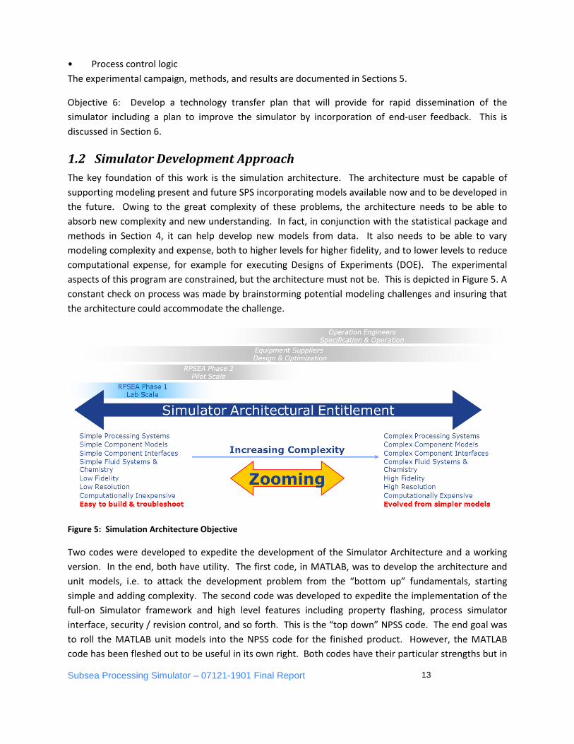
1.2 Simulator Development Approach The key foundation of this work is the simulation architecture. The architecture must be capable of supporting modeling present and future SPS incorporating models available now and to be developed in the future. Owing to the great complexity of these problems, the architecture needs to be able to absorb new complexity and new understanding. In fact, in conjunction with the statistical package and methods in Section 4, it can help develop new models from data. It also needs to be able to vary modeling complexity and expense, both to higher levels for higher fidelity, and to lower levels to reduce computational expense, for example for executing Designs of Experiments (DOE). The experimental aspects of this program are constrained, but the architecture must not be. This is depicted in Figure 5. A constant check on process was made by brainstorming potential modeling challenges and insuring that the architecture could accommodate the challenge.
Figure 5: Simulation Architecture Objective
Two codes were developed to expedite the development of the Simulator Architecture and a working version. In the end, both have utility. The first code, in MATLAB, was to develop the architecture and unit models, i.e. to attack the development problem from the “bottom up” fundamentals, starting simple and adding complexity. The second code was developed to expedite the implementation of the full-on Simulator framework and high level features including property flashing, process simulator interface, security / revision control, and so forth. This is the “top down” NPSS code. The end goal was to roll the MATLAB unit models into the NPSS code for the finished product. However, the MATLAB code has been fleshed out to be useful in its own right. Both codes have their particular strengths but in

Subsea Processing Simulator – 07121-1901 Final Report 14
practice the concepts and models are portable between the two, and there are ways to implement most of the features of each into the other.
1.3 Experimental Validation A horizontal three-phase gravity separator and a saltwater / oil / gas flow loop were built and used 1) to develop and tune unit models and 2) validate the overall simulation and associated methods. The model development was done using steady operating states. With these steady state models and additional models based on first principles, the Simulator ran transient cases which are compared to experimental data. The experimental campaign is described in Section 5.
2 MATLAB Simulator Version
2.1 Objectives As mentioned above, the MATLAB code was developed to attack the simulation problem from the bottom up. Particular needs were the architecture for the models and data structures—how they are created, how they interact, and how they are solved. As this architecture was created, a development effort was made on how to model the horizontal three-phase separator, and later the test loop and separator as a whole.
What follows is a documentation of the MATLAB architecture, which is more or less the same as is employed in the full-on NPSS version. A simple tutorial that gives examples of the key features can be found in Appendix 0. All required MATLAB files are embedded therein. The three phase separator & test loop files are found embedded in Section 5, also as a complete package, along with description.
Often it is the case that there are many ways to achieve the same purpose, including how best to divide the simulation problem into pieces, how to define unit models, when to create sub-models, how to solve systems, and so forth. The nomenclature is fairly well developed at this point, as this code has been used not only for RPSEA work but for some key GE internal programs. It is not always easy, particularly in the scripts, so tell what a set “tool” is and what custom code is. This is to be taken as a show of flexibility and capability to evolve. Code segments and model combinations that are useful can be pulled into new unit models and tools. It is anticipated as user groups develop and libraries are built, useful tools, conventions, and routines will emerge.
2.2 Simulator Infrastructure There are four things needed to run a MATLAB simulation: 1) The simulator code, 2) unit models, 3) a control file, and 4) a run script. Each of these is described below.
2.2.1 Simulator Code The first is the simulator code itself which is organized in several m-files. MATLAB needs to have a path set to these files for execution. They include a collection of files named Stat_*.m which are useful for

Subsea Processing Simulator – 07121-1901 Final Report 15
batch runs and statistical analyses and are discussed in Section 4. The remaining files are named Tool_*.m of which only the following are essential:
• Tool_BuildModel.m calls Tool_Read_Ctrl.m to load the Control File which contains the assembly of the model (more on this later) and then initializes the MATLAB data structures.
• Tool_RunCase.m executes the top level Unit Models as using default settings, what is specified in the Control File, what is specified in the run script, or what is directed in a unit model, whichever occurs latest. (As mentioned earlier, there are many ways to do the same thing. This is a feature!) It can be directed to iterate over the Unit Models or a subset thereof until convergence is obtained, or execute them once. It also sets up next-step working space in the data structures for transient and batch simulations.
The other tools are MATLAB code snippets that perform useful functions:
• Tool_RunCases.m takes a list of cases typically generated using the statistics package preprocessor and feeds them to Tool_RunCase.m for execution.
• Tool_PlotRun2D.m makes it easy to plot simulation results.
• Tool_PlotSlice.m also makes plots and is of particular use with batch runs / statistical package post-processing.
2.2.2 Unit Models Unit models are implemented as MATLAB functions. They exist to retrieve relevant information from the data structures, perform some computation, lookup, or call to an external program, etc., and then return their output in the correct locations in the data structures. With the use of standardized interfaces, the possibility of replacing, updating, enhancing models is easy. They can also be deployed hierarchically, i.e., a unit model can be used as a sub-model within another unit model. Unit models can be instanced. Tag based nomenclature is used to locate data for storage or retrieval. This can make the calls long, but easily decipherable.
2.2.3 Control File The control file contains the information for assembling the Unit Models into simulations. It contains a list of top level Unit Models and how they are connected. It contains a list of variables and their initial values as needed in the different structures. Finally, it can contain the methodology of executing the models.
2.2.4 Run Script The run script is a MATLAB m-file whose execution launches the building and execution of the simulation. This can be augmented to include any other operations deemed useful, such as code to implement various simulation cases or post-processing. If the MATLAB tools are used to set up batches and perform complex post-processing analyses, the script can be quite complex but very useful. Script segments can be relegated to m-files as is useful for organizational or sharing purposes.

Subsea Processing Simulator – 07121-1901 Final Report 16
2.3 RPSEA Simulator Architecture The fundamental building blocks of the RPSEA Simulator architecture are the Data Structure and Unit Models.
2.3.1 Data Structure At present the Data Structure contains four sub-structures organized by what they store:
The GB sub-structure is for constants. They can be modified, but only the last value is stored.
The Global sub-structure is for storing things that may vary with time.
The Stream sub-structure is for storing things that may vary with time and location, i.e., at the connections between top level unit models.
The Fluid sub-structure stores things that may vary with time, location, and by fluid.
These structures are convenient because they facilitate location of data using tags and minimize memory use while keeping the workplace clean and organized. Experience exists with adding and tracking data outside these structures. For example, custom structures are used in the three phase horizontal test separator simulations to track the motions of droplets and bubbles (and perhaps in the future, sand).
2.3.2 Unit Models Unit models start with a standard MATLAB function declaration. It is highly recommended that this is followed with documentation which states the model’s function, methodology, and variables that need to have been defined in the Control File. It should also document what unit models are employed as sub-models and define what the various outputs are. It is recommended that the documentation is followed with some boilerplate code that first copies the stream and fluid data entering the unit model to their corresponding locations on the unit model output. Otherwise stream components on which the unit model does not operate will be lost, having not been propagated downstream. Finally, the calculation block follows. This may be equations, look up tables, calls to external packages, etc. The key results are exported to their appropriate locations in the Data Structures. Top level unit models as defined in the Control File are executed as directed by the modeler via Tool_RunCase.m. Sub-Models are executed when called for by their host.
2.4 Comments The architecture is based on simple and minimalistic principles. Were it not so, the simulation developer would face unwanted constraints in solving problems. The typical approach to building a simulation is to start simple and get a model working. From this point complexity can be added, unit models can be organized and reorganized, and the simulation evolved into something comprehensive. The tutorial and test separation models are provided to give examples of this.

Subsea Processing Simulator – 07121-1901 Final Report 17
3 NPSS Simulator Version
3.1 Objectives The simulator framework should have the ability to:
Define the system as a network of component/elements that model the basic physics of the subsea processing system. Exchange information between different components/elements that define the overall system. Transfer Fluid streams from one component to another through reconfigurable ports. Model a generic stream that can comprise of Liquid, Gases and Solids that can exist in Discrete (bubbles, particles) and continuous mixed form. Capture the thermodynamics of the mixtures by having the ability to hook up commercial thermodynamic libraries such as Multiflash, HYSYS etc. Permit a multiple user concurrent model development through version control and managing different versions of the code for easy distribution and release. Permit model exchange across companies in joint development projects while still protecting the proprietary equations and data that are part of the models by encoding. Run in a batch mode so that statistical analysis can be done in an automated multi-processor environment.
3.1.1 Criterion for selecting the Platform Based on the above description, the list below summarizes the criterion to select the platform:
Model Build Environment (Ease, Customize, Flexibility and Capability) Component Model Library and Ease of Creating new Components Template Fluid Stream Models Thermodynamics & Flashing of Fluid Streams Ability to Call Other Commercial Packages (C++ / Java) Ability to be Integrated into Commercial Packages Version Control, History and Release Process Model Integrity and Exchange within Same Organization & Across Companies Costs for maintaining & deploying Framework
3.2 What is NPSS (Numerical Propulsion System Simulation)? Within NASA’s High Performance Computing and Communication (HPCC) program, the NASA Glenn Research Center (GRC) developed a large scale, detailed simulation environment for the analysis and design of aircraft engines called the Numerical Propulsion System Simulation (NPSS). NPSS was created as an object-oriented engineering environment for use in the analysis and design of complex systems and includes an open architecture with a flexible user interface. NPSS is a state of the art simulation tool that is becoming the Gold Standard for system modeling in the aerospace industry.
At its foundation, NPSS is a component-based object-oriented engine cycle simulator designed to perform cycle design, steady state and transient off-design performance prediction, test data matching, and many other traditional tasks of engine cycle simulation codes. Like traditional codes, an NPSS engine model is assembled from a collection of interconnected components, and controlled through the

Subsea Processing Simulator – 07121-1901 Final Report 18
implementation of an appropriate solution algorithm. Historically, limited computer resources restricted component representations used in these simulations to be simple characterizations of empirical test results, or the results of more sophisticated component models run separately. NPSS, however, is capable of calling upon more sophisticated component models directly. Using the computer industry’s Common Object Request Broker Architecture (CORBA) communication standard, NPSS can interact with external codes running on other computers distributed across a network. A work in progress, the advanced system architecture designed into NPSS will allow the marriage of design tools at varying levels of dimensional fidelity across multiple technology disciplines. Following are the basic out of the box capability of NPSS:
• All model definition through input file(s) • NIST (National Institute of Standards and Technology) compliant thermodynamic gas-properties
package • A sophisticated solver with auto-setup, constraints, and discontinuity handling • Steady state and transient system simulation • Flexible report generation • Built-in object-oriented programming language for user-definable components and functions • Support for distributed running of external code(s) via CORBA • Support for test data matching and analysis
This advanced performance analysis environment with an extensible framework provides an unprecedented level of interoperability and allows NPSS models to be readily interfaced with many commercial off the shelf software and customer developed applications. The ability to interface with multiple and diverse tools allows users to test the interactions between the system and specific subsystems and/or external system models. The powerful architecture enables NPSS to be used throughout the life cycle of the product. NPSS models are used in both preliminary and advanced design, development, test, manufacturing, operations, and more. These features make NPSS an invaluable tool for anyone creating products involving complex systems.
3.3 Simulation Structure
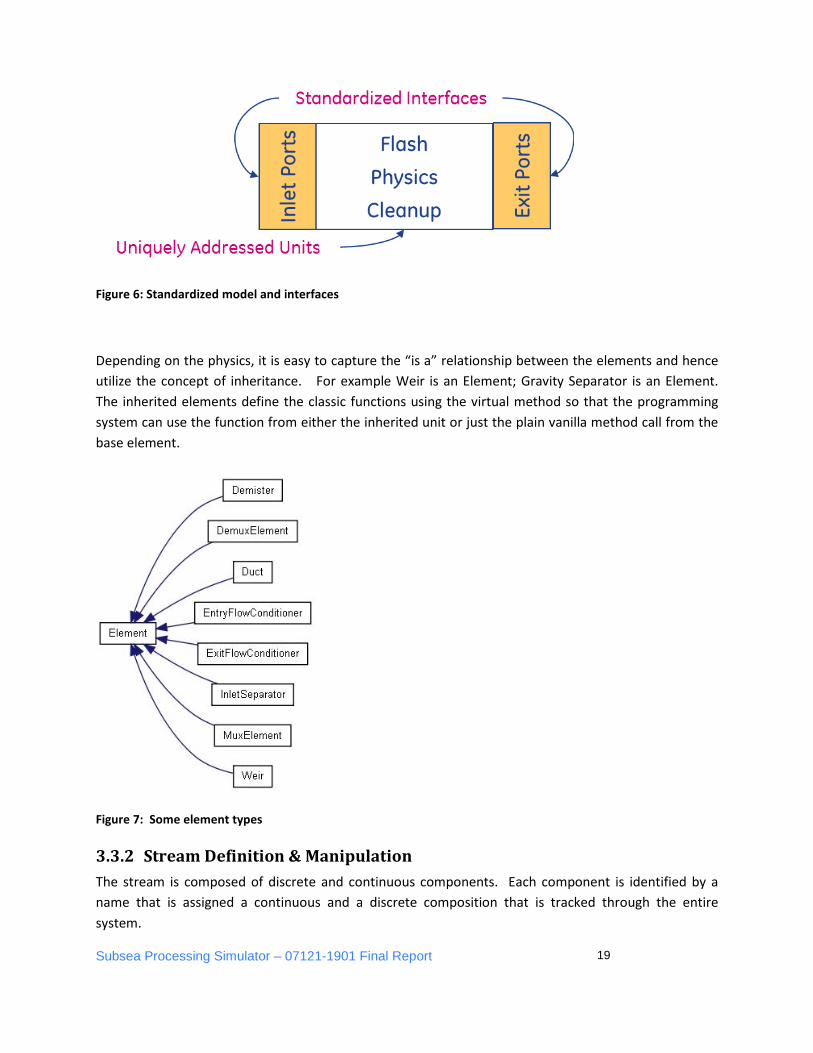
3.3.1 Hierarchical Units with Embedded Physics A fundamental unit called Element is defined to perform the most basic operation. The element has in/out ports that can accept streams, process them based on the physics defined inside the element.
The abstract unit comprises of an Inlet / Exit Port Array, Pre Calculate (Flash), Calculate (Physics) & Post Calculate (Cleanup). This unit is uniquely addressable in the overall system and its fields / properties can be extracted and used by any other portion of the system (Figure 6).
Subsea Processing Simulator – 07121-1901 Final Report 19
Figure 6: Standardized model and interfaces
Depending on the physics, it is easy to capture the “is a” relationship between the elements and hence utilize the concept of inheritance. For example Weir is an Element; Gravity Separator is an Element. The inherited elements define the classic functions using the virtual method so that the programming system can use the function from either the inherited unit or just the plain vanilla method call from the base element.
Figure 7: Some element types
3.3.2 Stream Definition & Manipulation The stream is composed of discrete and continuous components. Each component is identified by a name that is assigned a continuous and a discrete composition that is tracked through the entire system.
Subsea Processing Simulator – 07121-1901 Final Report 20
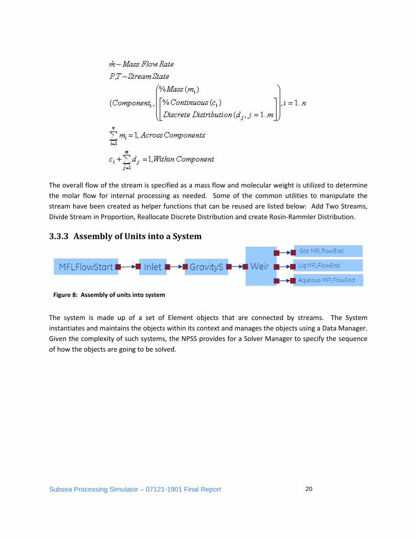
The overall flow of the stream is specified as a mass flow and molecular weight is utilized to determine the molar flow for internal processing as needed. Some of the common utilities to manipulate the stream have been created as helper functions that can be reused are listed below: Add Two Streams, Divide Stream in Proportion, Reallocate Discrete Distribution and create Rosin-Rammler Distribution.
3.3.3 Assembly of Units into a System
The system is made up of a set of Element objects that are connected by streams. The System instantiates and maintains the objects within its context and manages the objects using a Data Manager. Given the complexity of such systems, the NPSS provides for a Solver Manager to specify the sequence of how the objects are going to be solved.
Figure 8: Assembly of units into system

Subsea Processing Simulator – 07121-1901 Final Report 21
3.3.4 Library Management
Figure 9: Library management
In an interpreted programming context, the end user can create models locally in his sand box as text files. The users can package the models as a binary DLL, so that proprietary information such as design formulae or data need not be revealed to the end user. As with any version management system, the end user needs the capability to assemble the system from components that are in different versions. The context file help identify the valid set of components for that overall system revision.
3.3.5 Wrapping of External Modules into NPSS Framework This section describes the numerical zooming between a NPSS engine simulation and higher fidelity representation of the engine components. NPSS provides two software techniques to wrap higher fidelity code written in FORTRAN / C++ into a simulation component. One is based on the Dynamically Loadable Module (DLM) and the other is via the Common Object Request Broker Architecture (CORBA). This is a feature that will be used to wrap calls to external thermodynamic libraries for performing the flashing the hydrocarbon streams to determine the liquid & gaseous composition.
3.3.6 Integration of NPSS within other frameworks NPSS has the capability to package the System model as self-contained Customer Deck Modules. These self-contained entities can be exported to customers for testing it on their simulation environment in an encrypted format so that the proprietary design rules need not be divulged to outside world. This permits collaborative research between competitors on joint projects.
This capability can also be used to package the NPSS model so that it can be integrated with HYSYS/OLGA environments (Figure 10). The simulation environment has an Application Programming Interface by which the NPSS models can be invoked from an external package. The customer deck may be delivered with no encrypted files, or it may be delivered with one or more encrypted model files to be read in. It is also possible to read in non-encrypted files containing NPSS syntax. In addition, the customer deck can be run as a stand-alone program or called as a subroutine from another code.

Subsea Processing Simulator – 07121-1901 Final Report 22
Figure 10: RPSEA Interfacing with Process Simulator
3.4 Flashing of Fluid Properties
Flashing is one of the most common thermodynamic operations performed on the hydro-carbon fluid streams. The fundamental physics of flashing is captured in the Infochem’s Multiflash modules – we utilize the power of NPSS to incorporate the external thermodynamic modules to determine the stream state. Every port has a one to one linkage to a Flow Station which retains all the state information for a stream. Each FlowStation will internally relay the call to the Multiflash Thermodynamic module to calculate the properties which will then be saved as local variables in a FlowStation for that stream.
Figure 11: High level NPSS structure: Thermodynamics and Element/Port
Subsea Processing Simulator – 07121-1901 Final Report 23
The Element can directly access the information in the FlowStation through the ports and perform the calculations. For example, one can easily simulate InEnthalpic Mixing of two streams by just summing the enthalpies of the inlet streams and adding them inside the calculate module of the element. Finally, the cumulative property is relayed to the outlet port. It should be noted that all the calculations are done in the memory and hence very fast.
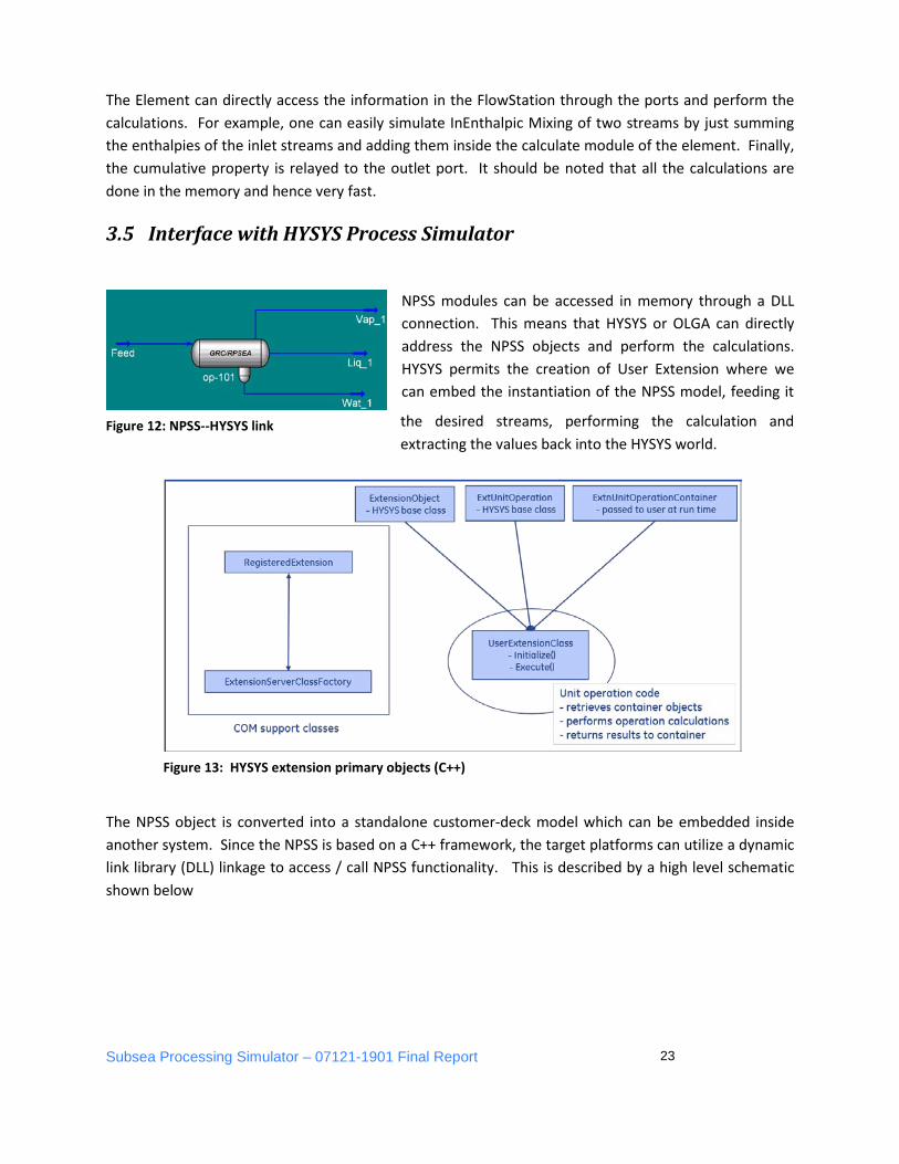
3.5 Interface with HYSYS Process Simulator
NPSS modules can be accessed in memory through a DLL connection. This means that HYSYS or OLGA can directly address the NPSS objects and perform the calculations. HYSYS permits the creation of User Extension where we can embed the instantiation of the NPSS model, feeding it
the desired streams, performing the calculation and extracting the values back into the HYSYS world.
The NPSS object is converted into a standalone customer-deck model which can be embedded inside another system. Since the NPSS is based on a C++ framework, the target platforms can utilize a dynamic link library (DLL) linkage to access / call NPSS functionality. This is described by a high level schematic shown below
Figure 12: NPSS--HYSYS link
Figure 13: HYSYS extension primary objects (C++)

Subsea Processing Simulator – 07121-1901 Final Report 24
3.6 Summary In summary, the NPSS simulator provides for the following advantages:
Increase modeling flexibility Improve productivity and accuracy earlier in the design process Reduce dependency on resident code experts Facilitate large scale and multi-platform system simulations Significantly reduce development time Decrease the risk of failure during development Reduce waste of materials and resources Support Plug-N-Play NPSS Internal Codes Eliminate inefficient date exchange by minimizing manual data transfers Reduce the cost of support, development, and training
4 Statistical Package Per the requirements of the RPSEA project, a statistical package has been developed to determine operational envelopes and probabilities of system success. This package consists of methods, tools, and example scripts for extracting the wanted information from the models. Due to the architecture of the RPSEA Simulator, particularly how all variables are treated similarly, the statistical package has two additional utilities of great importance: First, there is optimization of design / operation. Unit models may include physical, control, or other parameters that can be varied within batches of runs. Given one or more performance metrics, these parameters can be chosen such that performance is maximized. Example: choosing a separator vessel’s dimensions such that weight is minimized without an excessive performance hit. Second, there is the tuning of models, in which existing models are infused with
Figure 14: HYSYS / NPSS interactions

Subsea Processing Simulator – 07121-1901 Final Report 25
coefficients, whose values are found such that modeling errors are minimized. This key process improves model accuracy and generality, and permits mining of data to produce new / improved models which can then be adopted into the unit model library.
Figure 15 shows how the statistical tools interact with the simulator environment. A preprocessor can set up a batch of cases that are executed in the Simulator Environment, and/or the variable inputs can be implemented at the process simulator level. As the statistical package is presently implemented in MATLAB, the former case is the norm. For each simulation in the batch, the statistical tool receives results for post-processing. More accurately, all batch run results exist in the data structures, and it is known how to parse the data associated with each batch case. The statistical package tools and a script are then used to analyze the results, examine cause-and-effect and sensitivities, calculate operation envelopes and probabilistic metrics, optimize designs, and tune models.
Figure 15: Interface of Characterization tools with Simulator
4.1 Pre-Processor The sole purpose of the pre-processor is to create a list of cases to be run. This list is created as a two-dimensional array in Stat.Cases in which each column represents a single case to be run, and each row represents a different variable. Any GB, Global, Stream, or Fluid variable can be varied. A companion structure Stat.ID indicates which variable is associated with each row of Stat.Cases, as well as the parameters associated with each variable, and an identifying flag. Given these two arrays, Tool_RunCases can then be invoked, which will column by column (case by case) load the variables associated with that case (using Stat.ID as the map), overwriting prior definitions in the control file, and

Subsea Processing Simulator – 07121-1901 Final Report 26
executing the simulation using Tool_RunCase. Results from subsequent cases are appended to the variable structures for subsequent parsing and analysis, using tools discussed below.
Stat_SetCases was developed to create the batch of cases in Stat.Cases and associated annotation in Stat.ID. “help Stat.SetCases” will bring up the syntax as needed. In short, the user creates Stat.ID which includes on each row a variable that is to be varied, the method by which it is varied, and a flag to identify what type of variable it is.
The first method of variation is probabilistic. A property such as a stream or fluid compositional property may be randomly chosen using a cumulative distribution function (CDF). If there are more than one probabilistically selected variable, a correlation matrix is required which describes how the variables are related to each other. Using this and a copula, a user selected number of cases are created according to the statistical distribution. The various combinations represent statistically likely combinations. A typical CDF and PDF for 5 different types of distributions are shown in Figure 16. In Stat.ID, these variables are flagged with an ‘R’
Figure 16: Statistical Distributions

Subsea Processing Simulator – 07121-1901 Final Report 27
Next, variables can be varied across a user defined range, i.e., from a minimum value to maximum value in steps of some amount. This is useful for everything from screening designs to finding operational envelopes to optimizing and so forth. The user can put in a list of custom values if needed. Two flags are used, though others can be defined: ‘G’ is for ‘gridded’ variables that are expected to fluctuate over the course of operations and thus may have statistical probabilities associated with each value during post-processing, and ‘P’ for parameters such as those for different physical system designs, controls, model tuning factors, etc.
By way of example, Figure 17 shows a three dimensional set of cases below. Each point represents an individual test case. Note, as shown in the figure, the same random values for the random variable(s) are used for each combination of the other grid/parameter variables. This makes it possible to look at slices of data, i.e., in which the analysis covers a subset of cases associated with one value for the random variable. If different random values were chosen for each combination of the other variables, looking at and analyzing slices would not be possible.
Batches may have any number of variables.
Figure 17: Inputs combinations. Each dot represents a simulation case.
The process of defining batches of simulations can be easily customized as needed via script. For example, for the RPSEA horizontal separator work, the first variables are to match the actual experimental inputs from the tests. First, the experimental data (the test conditions—flow rate, fluid properties, etc.) are loaded into Stat.Cases, and Stat.ID is annotated to show what variable is associated with each row. After defining random, grid, and parameter variables and specifying their distributions, Stat_SetCases is called, which permutes the experimental variable values across all the chosen model parameters to be varied—in this case typically model tuning parameters. The flag for the experimental values from the data files is flagged with an ‘X’. These and other flags are useful in post-processing for automating the selection of rows of various types, as will be shown later. The flags are more for scripting convenience as the row labels are descriptive.

Subsea Processing Simulator – 07121-1901 Final Report 28
4.2 Batch Execution As mentioned above, given the list of cases (Stat.Cases) and the associated variables (Stat.ID), Tool_RunCases will execute all the simulations. The results of each simulation are appended to the various data structures. For steady state runs, that means the nth data column (same index as “time”) corresponds to the nth simulation case. For transient runs, there will be sequential blocks of data. The beginning of each new block is easily discerned as the time variable is reset to zero. In any case, the data structure index associated with time in a single run is now associated with time and simulation case.
4.3 Post-processor All simulation data from the batch is maintained in the usual data structures. Next, the typical step is to create a script to perform the wanted post-processing. The first though optional step is to complete the statistical description of the simulation inputs, i.e., for the ‘Gridded variables flagged with the ‘G.’ The randomly distributed ‘R’ variables already have a statistical description, and the ‘P’ parameter variables represent different instances—parallel realities, if you will. The execution of this tool is required for statistical analyses. The statistical description for the ‘G’ variables is given in much the same way as used in the pre-processor (see help Stat_PostStatistics) and requires a correlation matrix now sized to include the ’R’ and ‘G’ variables. Upon execution, this tool appends to Stat.Data (and annotates Stats.ID) the probability of each case (‘A’) and the ‘volume’ represented by that case (‘D’). To the extent that the variable ranges span the probable extent, integration of probabilities * volumes (i.e., the ‘volume’ under the probability distribution function ‘surface’) will numerically approximate 1. These probability and associated ‘volumes’ associated with each of the ‘R’ and ‘G’ variables are necessary for calculating probabilities / time percentages of success, net present values (NPV), and the like, which are extremely useful for characterizing system performance, optimizing designs, and so forth. For example, if the oil flow from operations at each case is known from modeling, and this value is multiplied by that case’s probability and ‘volume’, and this is summed over all cases (associated with one design parameter set, of course), a measure of present value results.
Next, it is necessary to extract the simulation results to be analyzed. Since there is one set of results per case, and Stat.Cases already has some of the requisite data—the inputs—it only makes sense to pull metrics from the results and append them to Stat.Cases, noting what each new row is in Stat.ID. For example, in a steady state batch, an oil-in-water fraction can be calculated for a water outlet for each case. This is done using the same tag based nomenclature as is used for accessing the data structures in the unit models. If each case is a transient run, there is some additional work to define metrics. Is the metric based on the last time step of the simulation? After some key event? An average over some time? All the data is available, but the user has to figure out the code to get what is wanted.
With Stat.Cases & Stat.ID containing the simulation inputs and results, one can make plots to explore the results. Tool_PlotSlice allows the user to select one, two, or three of the variables by row number and generate a histogram, 2-D scatter plot, or 3-D scatter and surf plots, respectively. Data can be filtered prior to plotting. The necessary syntax will show by typing “help Tool_PlotSlice.” Figure 18
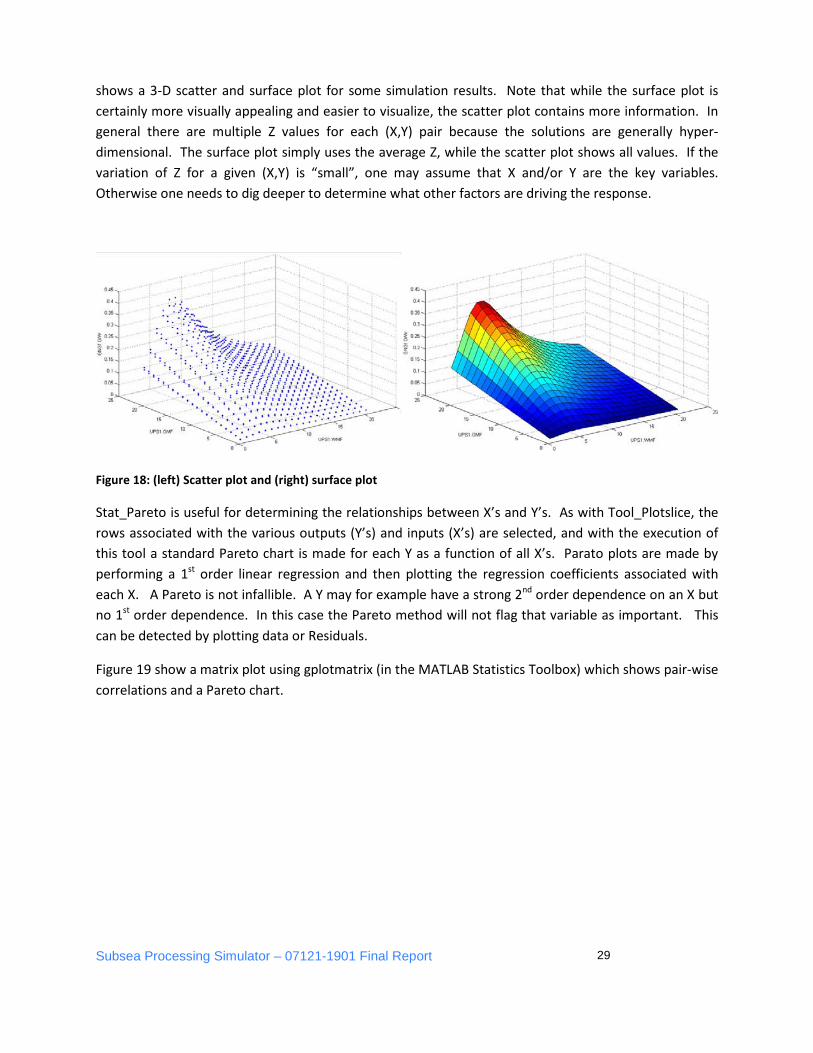
Subsea Processing Simulator – 07121-1901 Final Report 29
shows a 3-D scatter and surface plot for some simulation results. Note that while the surface plot is certainly more visually appealing and easier to visualize, the scatter plot contains more information. In general there are multiple Z values for each (X,Y) pair because the solutions are generally hyper-dimensional. The surface plot simply uses the average Z, while the scatter plot shows all values. If the variation of Z for a given (X,Y) is “small”, one may assume that X and/or Y are the key variables. Otherwise one needs to dig deeper to determine what other factors are driving the response.
Figure 18: (left) Scatter plot and (right) surface plot
Stat_Pareto is useful for determining the relationships between X’s and Y’s. As with Tool_Plotslice, the rows associated with the various outputs (Y’s) and inputs (X’s) are selected, and with the execution of this tool a standard Pareto chart is made for each Y as a function of all X’s. Parato plots are made by performing a 1st order linear regression and then plotting the regression coefficients associated with each X. A Pareto is not infallible. A Y may for example have a strong 2nd order dependence on an X but no 1st order dependence. In this case the Pareto method will not flag that variable as important. This can be detected by plotting data or Residuals.
Figure 19 show a matrix plot using gplotmatrix (in the MATLAB Statistics Toolbox) which shows pair-wise correlations and a Pareto chart.

Subsea Processing Simulator – 07121-1901 Final Report 30
Figure 19: Graphical correlation tools
The next topic is the determination of operational envelopes. Stat_GoNoGoEnvelop looks for lines in Stat.ID in which the flag (in the 8th column) is a ‘B’ The argument in the 5th column is a threshold, and the 6th is ‘1’ if ‘higher than the threshold’ is a ‘Go’ or ‘-1’ if ‘lower than the threshold’ is a ‘Go’. Execution of Stat_GoNoGoEnvelope appends to Stat.Data (and annotates Stat.ID) with a row (Flag: ‘C’), corresponding to each line of interest that contains 1’s and 0’s for each case designating a ‘Go’ (success!) or ‘No-Go’ (failure!) for each case. Finally, it appends a row (Flag: ‘E’) that contains 1’s, where all the Booleans are 1, otherwise 0. Figure 20 shows the process. For some metric (left), a threshold is defined (red line) and a map created showing success and failure. Appreciate these simple plots, because in general the analyses will be hyper-dimensional.
Figure 20: Generation of Go-No Go Map
If post-processing statistics has been applied (Stat_PostStatistics—described above) and there are design parameters being varied (from pre-processor, flagged with a ‘P’), Stat_GoNoGoEnvelope will also consider each set of parameter cases one at a time, and in short multiply the Go No-Go Boolean surface by the probability surface times case volume and integrate to get the probability of each design to meet the various metrics. Voila! One can use this along with other metrics (cost of each design, weight of each design, etc) to pick the optimal design. Whereas Stat.Cases has one column for each case that is run, these results will have one column for each permutation of design parameters ‘P’. Hence new structures are created: Stats.ParaSet and Stat.ParaID with this data. They are in every way analogous to

Subsea Processing Simulator – 07121-1901 Final Report 31
Stat.Cases and Stat.ID respectively and can be examined using Tool_PlotSlice and Stat_Pareto in the expected manner. Figure 21 shows an example in which the Go / No-Go map of Figure 20 is multiplied by the probabilities associated with each of the cases. Integration under this surface, done by multiplying the Go / No-Go Boolean by the probability and volume associated for each state associated with one parameter set and summed, gives the probability of success.
Figure 21: Probability of success
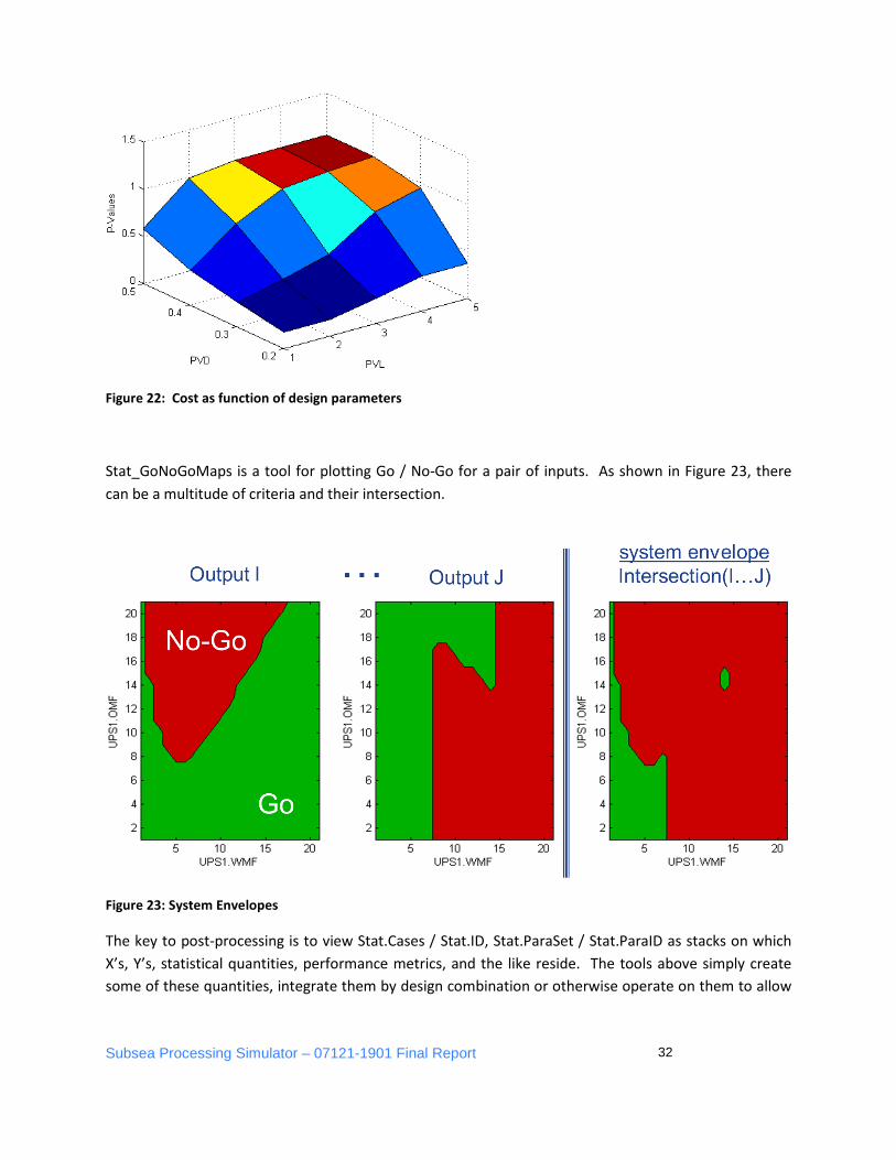
Figure 22 shows a plot in which the above has been done for each design parameter permutation by Stat_GoNoGoEnvelope, and the probability of success is plotted verses design parameters using Tool_PlotSlice. The highest point is the optimal design with respect to the defined metric.
Subsea Processing Simulator – 07121-1901 Final Report 32
Figure 22: Cost as function of design parameters
Stat_GoNoGoMaps is a tool for plotting Go / No-Go for a pair of inputs. As shown in Figure 23, there can be a multitude of criteria and their intersection.
Figure 23: System Envelopes
The key to post-processing is to view Stat.Cases / Stat.ID, Stat.ParaSet / Stat.ParaID as stacks on which X’s, Y’s, statistical quantities, performance metrics, and the like reside. The tools above simply create some of these quantities, integrate them by design combination or otherwise operate on them to allow
Subsea Processing Simulator – 07121-1901 Final Report 33
visualization, reduction, optimization, or the like. While such analyses may seem complex when taken as a whole, the steps when broken down are fairly straight forward.
As mentioned before, there is no real line between tools and scripts. Scripts morph into tools inasmuch as they obtain general usefulness. In between these limits are templates.
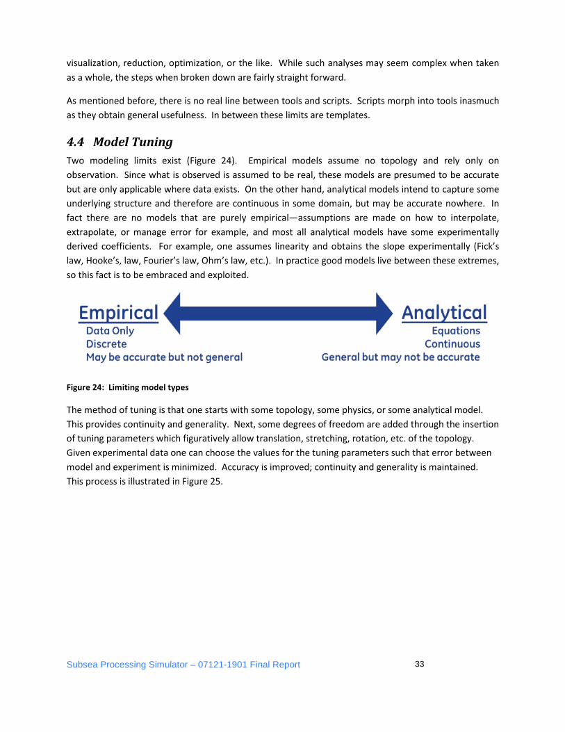
4.4 Model Tuning Two modeling limits exist (Figure 24). Empirical models assume no topology and rely only on observation. Since what is observed is assumed to be real, these models are presumed to be accurate but are only applicable where data exists. On the other hand, analytical models intend to capture some underlying structure and therefore are continuous in some domain, but may be accurate nowhere. In fact there are no models that are purely empirical—assumptions are made on how to interpolate, extrapolate, or manage error for example, and most all analytical models have some experimentally derived coefficients. For example, one assumes linearity and obtains the slope experimentally (Fick’s law, Hooke’s, law, Fourier’s law, Ohm’s law, etc.). In practice good models live between these extremes, so this fact is to be embraced and exploited.
Figure 24: Limiting model types
The method of tuning is that one starts with some topology, some physics, or some analytical model. This provides continuity and generality. Next, some degrees of freedom are added through the insertion of tuning parameters which figuratively allow translation, stretching, rotation, etc. of the topology. Given experimental data one can choose the values for the tuning parameters such that error between model and experiment is minimized. Accuracy is improved; continuity and generality is maintained. This process is illustrated in Figure 25.

Subsea Processing Simulator – 07121-1901 Final Report 34
Figure 25: Tuning process
Recognizing that this process would be essential for the validation of the RPSEA Simulator and invaluable for creating models in general, an effort was commenced to develop these tools until it was realized that they already exist as part of the statistical package. Tuning parameters are isomorphic with design parameters, and thus the same optimization methods apply.
Some notes: Simpler models are easier to tune, being less topologically rigid and complex. It is vastly preferred to tune aspects that are not well understood as opposed to things relatively known such as dimensions, natural constants, etc).
Tuning is a process of generalizing. One could find a set of tuning parameters using oil A, then repeat the process for oil B. Tuning parameters that remain unchanged between the two oils would seem to be independent of that which makes the oils different. On the other hand, if the two oils have different viscosities for example, one could take the varying tuning parameters to be functions of viscosity. Implementing this function pops the model up a level in generality that now includes arbitrary viscosity (over some range) which can then be further tested, developed, and validated. Modeling, data, and tuning produces new models of increasing generality and accuracy. The goal of this Simulator and package is to soak up all available knowledge and understanding and grow in capability.

Subsea Processing Simulator – 07121-1901 Final Report 35
5 Experimental Validation
5.1 Test Objectives As stated in Section 1, the objective is to develop a lab-scale test facility and testing protocols for the validation of both the analytical models and the simulator performance; to develop a methodology and associated procedures for using the Simulator to determine the operational envelope for various process designs; and Using the lab-scale test facility and protocol, validate the simulator performance by executing a test plan to evaluate over a wide range of conditions. This section describes the test facility, the experimental test separator and system, the Simulator models of the same, and the procedures used for model development and overall simulation validation.
5.2 Flow Loop Design A schematic of the flow loop is shown in Figure 26. It consists of a three-phase (gas / oil / fresh (salt) water) facility featuring a large, atmospheric pressure, polishing tank which is the main reservoir of test fluids and separates them for controlled circulation through the test loop. Circulation is controlled by separate pumps for the oil and fresh (salt) water, and a compressor for the gas. A globe valve is installed downstream of the mixing header to create shear in the flow and further mix it avoiding stratification. At the inlet of the test section another ball valve is installed, which this is partially opened to promote mixing and droplet / bubble creation. The compressed gas is taken from the top of the atmospheric pressure tank. The oil and water in the test separator are regulated using the level indicators and level control valves. After the test separator, the fluids are recirculated back to the polishing tank in separate gas / oil / fresh (salt) water lines to force further separation in the polishing tank.
5.2.1 Specifications The test separator and the flow loop have been design and built for a pressure rating of 16 bar at 20° C. Maximum oil and water flow rates are 70 m3/hour each, and maximum gas rate is 270 m3/hour. The range of operating temperatures is 4 to 40° C.
5.2.2 Control System and Instrumentation The test rig’s automation system consists of the LabView control system and the instrumentation system as shown in Figure 27.
Control System Features:
• LabView provides an extremely flexible solution for integration of new test equipment. • Online trending of user-selected data. • Logging of all test data. • Alarm and shutdown functionality. • Ethernet-based IO for easy installation.

Subsea Processing Simulator – 07121-1901 Final Report 36
Figure 26: Experimental flow loop schematic

Subsea Processing Simulator – 07121-1901 Final Report 37
Fig 27: Control System programmed in LabView
Instrumentation includes the following. There is a flow meter and an electrically actuated flow control valve at the outlet of each of the pumps and compressor to enable for control of the circulation of the fluids. Pressure and temperature instruments are mounted at different points on the four inch pipe. Level indicators and electrically actuated level control valves are installed on the test separator to regulate the fluid levels. A pressure control valve is also installed at the test separator in order to control the pressure to the desired operating value. As required, sight glasses such as that shown in Figure 28 are installed in the test rig at inlet and outlet of the test separator to visualize the fluid from three directions (top, and two sides). Sampling points are also provided at both atmospheric pressure tank and test separator.

Subsea Processing Simulator – 07121-1901 Final Report 38
Fig 28: Flow loop sight glasses
Each of the motors for the water and oil pump is controlled based on the Direct Torque Control method. Two-phase current and direct current link voltage are measured and used for the control. The third phase current is measured for earth fault control.
The level instrumentations for the oil and water phases inside the test separator are floater made by Orion Instruments. The range is 0 – 50 cm on the oil side and 0 – 40 cm on the water side. The floating chamber is mounted to the side of separator vessel, and as the liquid rises and falls, a float with a built in magnetic system inside the external chamber rises and falls with the liquid level. The chamber is completely sealed so that the only moving part of the apparatus is the float. A sketch of the instrument is shown in Figure 29.
On the exterior side of the chamber is the magnetic indicator display, a column of magnetic rollers which are white on one side and red on the other side. As the float moves up and down, the concentrated magnetic field of the float magnet pulls the rollers through a rotation of 180 degrees, thus changing their colors. As the float rises, the color is changed from white to red, and as the float falls, the color is changed back to white again. Thus, the level of liquid in the tank is constantly represented by the red column. This is also connected to LabView for easy control.
Fig. 29. Schematic of Level Instrument

Subsea Processing Simulator – 07121-1901 Final Report 39
The pressure meters are shown in Figure 30 and made by GE Druck, with a range of 20 mbar – 1400 bar. At the heart of the instrument is micro-machined silicon sensing element. Micro machining defines the thickness and the area of the silicon which forms the pressure sensitive diaphragm. A fully active four-arm strain gauge bridge is diffused into the appropriate region. The basic sensor is housed within the high integrity glass to metal seal, providing both electrical and physical isolation from the pressure media. The electronic assembly utilizes microprocessor technology to create a compact circuit with the minimum of components while producing extremely stable signal unaffected by the shift in ambient temperature.
Fig. 30. Pressure sensors
The flow instrumentations for the liquids are a series of Coriolis flow meters made by Krohne Coriolis with a capacity of 100m3/hr, and shown in Figure 31. The measuring is based on the Coriolis principle. A Coriolis single tube mass flowmeter consists of a single measuring tube 1, a drive coil 2, and two sensors 3 and 4 that are positioned either side of the drive coil. When the meter is energised, the drive coil vibrates the measuring tube causing it to oscillate and produce a sine wave 3; the sine wave is monitored by the two sensors (OPTIMASS 1000).
(a)

Subsea Processing Simulator – 07121-1901 Final Report 40
(b) (c) Fig. 31. Coriolis flow meter (a) at rest, (b) energized, and (c) energized with process flow.
When a fluid or gas passes through the tube, the Coriolis Effect causes a phase shift in the sine wave that is detected by the two sensors. This phase shift is directly proportional to the mass flow. Density measurement is made by evaluation of the frequency of vibration and temperature measurement is made using a Pt500 sensor. For air flow measurement, Krohne Vortex Flowmeter was used, with a capacity of 20m3/hr. The functional principle is based on ISP (Intelligent Signal Processing).
5.3 Test Separator The RPSEA test separator is 6m long and 730 mm ID, with flanged flat end-plates. It has one single inlet and three outlets, one for oil, one for water, and the last outlet for gas. An inlet vane is used as the inlet device and a weir plate mounted at 0.75 m upstream of the seam at the outlet end of the tank to cover 70 percent of the area. Figure 32 shows a simple sketch of the test separator and an actual picture of the separator at the facility.
Weir Gas exit
Oil exit Water exit

Subsea Processing Simulator – 07121-1901 Final Report 41
Figure 32: RPSEA test separator
5.4 Test Program The fluids used for the test were the model fluid Exxsol D80, fresh water, and salt water. The properties of the model oil are:
Manufacturer: ExxonMobil Chemical Exxsol D80
Major components: Normal Paraffins, Isoparaffins and Cycloparaffins Specific Gravity: 0.79 Viscosity: 1.71 cP @ 25 C Surface tension @ 25 degC 26.3 mN/m Behavior over time: When Exxsol D80 and water and in contact, the oil tends to deteriorate
over time with growth of algae in the oil, which supposedly changes the chemical properties of the mixture.
Typical produced oils in the GOM include the lighter Miocene, with a specific gravity ranging from 0.6 to 0.85 and a viscosity of 0.5 to 2 cP, and the Paleogene with a specific gravity ranging from 0.8 to 0.9 and a viscosity of 1 to 50 cP The experiment test matrix was designed to vary the oil flow rate, water flow rate, and oil and water levels in the test separator. Each of the four variables is set to three different levels, giving a total of 81 test runs for a full factorial design. Some test runs were not successfully carried out due to tight level sitting that resulted in a very stable emulsion formation.
A first batch was run with oil and fresh water, and a second, reduced, batch was run with salt water. For this, a concentration of 35 g/l of salt in water was used. The grams of salt required for the experiment was calculated based on the volume of fresh water in the polishing tank. A separate mixing tank was

Subsea Processing Simulator – 07121-1901 Final Report 42
provided for mixing the salt before being pumped back to the polishing tank. After the salt had been mixed, the water pump was used to circulate the salt water for a homogeneous mixture of salt. A conductivity meter was used for verification of the salinity of the water. On confirmation of the salinity required, the salt water is applied for the experiment. Variables and levels used for the design of the test matrix:
Oil test separator (cm): 40, 44, 50 Water test separator (cm): 10, 17, 25 Oil flow rate (m3/hr): 10, 15, 20 Water flow rate (m3/hr): 10, 15, 20
The entire test matrix is attached as an annex to this document.
The following procedure was followed when running different points of the test matrix:
Test Procedure
1 Input the conditions to the software controlling the loop as indicated in the matrix for the test.
2 With variables plotted in the software, allow the loop to attain steady state condition.
3 Once steady state is attained, flush oil sampling point from the test separator to remove entrained fluid.
Take oil sample from the test separator from oil sampling point.

Subsea Processing Simulator – 07121-1901 Final Report 43
5 Repeat #3 for water sampling point for RPSEA separator.
6 Take water sample from the test separator water sampling point.
7 Visually check oil outlet sight glass, if possible take pictures.
8 Visually check water outlet sight glass, if possible take pictures.
9 Visually check gas outlet sight glass. Comment on gas carry over
10 Allow time for samples to separate, so that readings can be taken.
11 Record your reading.
12 Dispose of sample fluid after the reading has been recorded
13 Thoroughly clean vases.
14 Repeat for next test matrix point.
For every test case, oil and water samples were collected in order to check for the separation efficiency. The sampling procedure was:
Sampling Procedure
1 Allow system to attain steady state.
2 Flush the Polishing separator sampling points for both oil and water outlets.
3 Take sample from the Polishing separator outlets, to confirm that there is no emulsion in the system.
4 Flush RPSEA separator sampling points.
5 Take samples from both oil and water outlet of RPSEA separator using calibrated bottles.
6 Allow samples to stabilize for reading.
7 Go to 1 for next test run
5.5 Test Results Assuming the separation efficiency is affected only by the gravity force, the retention time for test run depends on the pump flow rate and phase level in the RPSEA separator. These physical variables will combine with the different physics of the separation to give an outcome for the test. Test results were only quantified in terms of water carry over in oil line and oil carry over in water line. Figure 33 shows the plot of the test results with phase carryover vs. retention time.

Subsea Processing Simulator – 07121-1901 Final Report 44
Figure 33: showing plot of carryover vs. Retention time for different level settings in the test separator
Since retention time does not collapse the data presented in Figure 33, we can conclude that physical processes other than gravity separation are taking place in these experiments. It is suggested to consider surface tension due to pressure changes or more complex physical models for the gravity separation (i.e., considering droplet packing, foam formation, film drainage, etc.).
As will be shown in the following sections, some data points did not follow trends typical of the majority of the data. For these “bad data” cases, photos such as that in Figure 34 for Run 63 show the oil outlet for this case. There is a lot of foam in the oil, and it might be possible to say that there are two characteristic sizes (foam with very small air bubbles, and also very large air bubbles). Not being able to break the foam layer is a sign of a very short residence time. Formation of foam is ‘new physics’ that affected data behavior and matches; other cases generally did not foam.
Pictures were not taken for the rest of the cases (e.g., Runs 3, 32, 40, 54, 65, 68), as it was impossible to see through the sight glass. This might be considered as a sign of “very bad” separation. While turbidity tests are run at platforms for a quick assessment of the water/oil separation quality, these can be misleading because turbidity depends not only on oil-in-water content, but also on the droplet size and the droplets’ combined light dispersion index.
0
10
20
30
40
50
60
70
80
0 20 40 60 80 100 120 140Retention Time (Sec/m2)
Car
ryov
er Water CaseOil Case
(%)

Subsea Processing Simulator – 07121-1901 Final Report 45
Fig. 34 – Run 63. Oil outlet showing foam with different characteristic sizes.
Figure 35 shows two different pictures from the oil outlet: Figure 35 (a) was taken from run 44 in which there was no water measured in the oil outlet. The oil is so clear that the three light sources are visible through the glass. There is a small amount of water droplets/foam trapped in the sight glass frame and the cleaning pipe, but those agglomerations were stable and didn’t detach for case a as long as the experiment was run. Figure 35 (b) was taken for case 49, which yielded 20 percent water-in-oil content. The mixed water is visible as whiter “lumps” in which no droplet size was recognizable.
(a) (b)
Figure 35. Oil outlet, with 0% WiO (a), and 20% WiO (b).
(a) Note: Bubbles are stuck from previous experiments in dead zones; fluid otherwise is very clear (b) Note: white is ‘chunks’ of water; grey is unstable emulsion
There were no pictures taken from the water outlet as the sight glass was either completely clear for the 0 percent oil-in-water cases, or completely opaque for the rest of the cases. No droplet size was recognizable from those runs (either too small for the “naked” eye, or too big forming lumps).
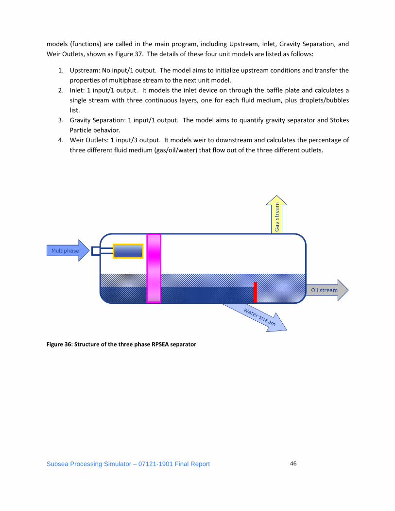
5.6 Simulation Setup As described in Section 5.3, the basic structure of the three phase RPSEA separator is shown as Figure 36. Gas, oil, and water are separated and flow out from the corresponding outlet. Four top-level unit
Subsea Processing Simulator – 07121-1901 Final Report 46
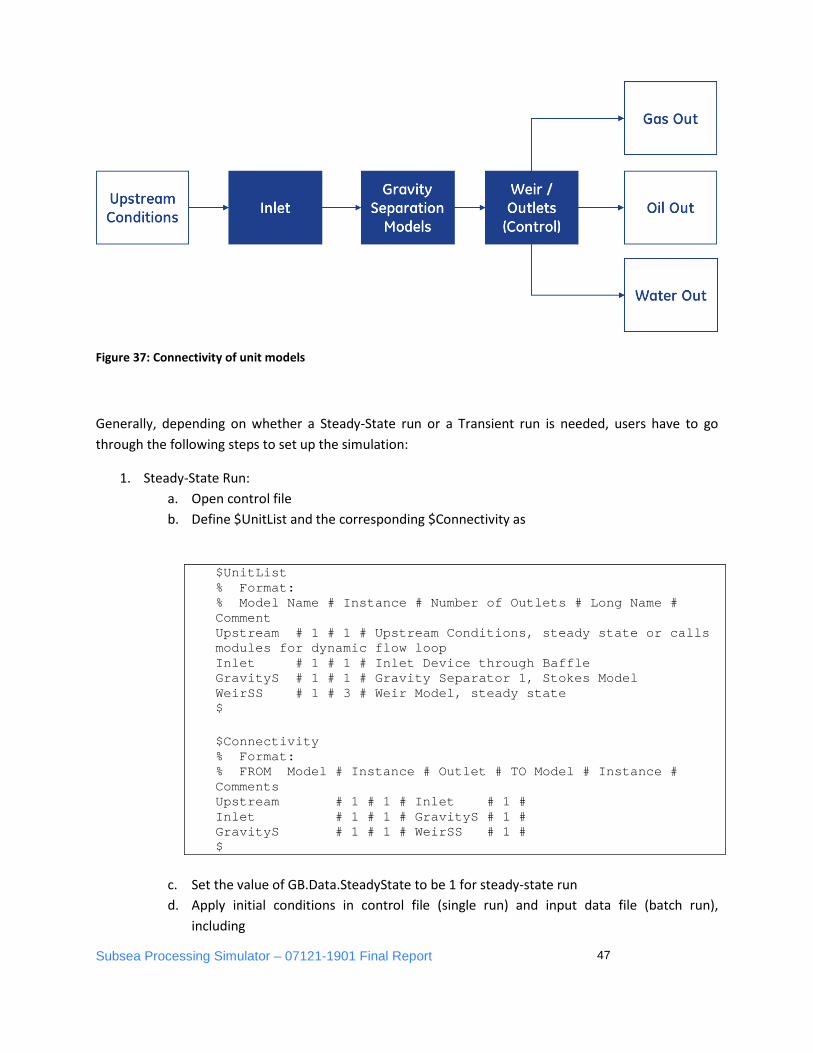
models (functions) are called in the main program, including Upstream, Inlet, Gravity Separation, and Weir Outlets, shown as Figure 37. The details of these four unit models are listed as follows:
1. Upstream: No input/1 output. The model aims to initialize upstream conditions and transfer the properties of multiphase stream to the next unit model.
2. Inlet: 1 input/1 output. It models the inlet device on through the baffle plate and calculates a single stream with three continuous layers, one for each fluid medium, plus droplets/bubbles list.
3. Gravity Separation: 1 input/1 output. The model aims to quantify gravity separator and Stokes Particle behavior.
4. Weir Outlets: 1 input/3 output. It models weir to downstream and calculates the percentage of three different fluid medium (gas/oil/water) that flow out of the three different outlets.
Figure 36: Structure of the three phase RPSEA separator
Subsea Processing Simulator – 07121-1901 Final Report 47
Figure 37: Connectivity of unit models
Generally, depending on whether a Steady-State run or a Transient run is needed, users have to go through the following steps to set up the simulation:
1. Steady-State Run: a. Open control file b. Define $UnitList and the corresponding $Connectivity as
$UnitList % Format: % Model Name # Instance # Number of Outlets # Long Name # Comment Upstream # 1 # 1 # Upstream Conditions, steady state or calls modules for dynamic flow loop Inlet # 1 # 1 # Inlet Device through Baffle GravityS # 1 # 1 # Gravity Separator 1, Stokes Model WeirSS # 1 # 3 # Weir Model, steady state $ $Connectivity % Format: % FROM Model # Instance # Outlet # TO Model # Instance # Comments Upstream # 1 # 1 # Inlet # 1 # Inlet # 1 # 1 # GravityS # 1 # GravityS # 1 # 1 # WeirSS # 1 # $
c. Set the value of GB.Data.SteadyState to be 1 for steady-state run d. Apply initial conditions in control file (single run) and input data file (batch run),
including

Subsea Processing Simulator – 07121-1901 Final Report 48
% Conditions P_in # value # Upstream Pressure [bara] T_in # value # Upstream Temperature [C] Q_in # value # Total Flow Rate [m^3/hr] GVF_in # value # Inlet GVF [] WC_in # value # Inlet Water Cut [] O_rho # value # Oil Density [kg/m^3] O_visc # value # Oil Absolute Viscosity [cP] G_visc # value # Gas Absolute Viscosity [cP] Level_O # value # [(0-1)] Oil Level # Oil-Gas Interface Level (2D model ~ area ratio) Level_W # value # [(0-1)] Water Level # Water-Oil Interface Level (2D model ~ area ratio) % Geometry GSH # value # Gravity Separator effective height [m] GSL(Instance) # value # Gravity Separator effective length [m] for each instance GSW(Instance) # value # Gravity Separator effective width [m] for each instance Gravity_DZ(Instance) # value # Gravity Separator DZ for droplet tracking [mm] for each instance
e. Define $StreamVarList, $FluidList and $FluidPropList as
$StreamVarList % Format: % Name # e/i (extensive or intensive) # Long Name Press # i # [bara] Static Pressure Temp # i # [C] Temperature $ $FluidList %Format: % Name # Phase (gas, liquid, solid) # Long Name Gas # gas # Air Oil # liquid # Oil Water # liquid # Salt Water $ $FluidPropList %Format: % Name # Long Name Density # [kg/m^3] Density Viscosity # [cP] Viscosity MFR # [kg/s] Mass Flow Rate CONTINUOUS Phase Max_Dia # [miocron] Max Droplet Diameter $

Subsea Processing Simulator – 07121-1901 Final Report 49
2. Transient Run: a. Open control file b. Define $UnitList and the corresponding $Connectivity same as Steady-state run c. Set the value of GB.Data.SteadyState to be 0 for transient run d. Apply initial conditions in control file (single run) and input data file (batch run),
including
% Run Setup SetPoint_OG # value # [(0-1)] Set Point for Gas-Oil Interface SetPoint_WO # value # [(0-1)] Set Point for Oil-Water Interface SetPoint_P # value # [bara] Set Point for pressure SetPoint_Q # value # [gpm] Set Point for Flow Rate SetPoint_WC # value # [(0-1)] Set Point for water cut SetPoint_GVF # value # [(0-1)] Set Point for Gas Volume Fraction SetTime_OG # value # [s] Time associated with SetPoint_OG SetTime_WO # value # [s] Time associated with SetPoint_WO SetTime_P # value # [s] Time associated with SetPoint_P SetTime_Q # value # [s] Time associated with SetPoint_Q SetTime_WC # value # [s] Time associated with SetPoint_WC SetTime_GVF # value # [s] Time associated with SetPoint_GVF % Water Pump WP_PID_On # Input # [] 1=PID controlled, 0 is manual setpoint WP_PID_MS # Input # [] Manual Setpoint for water pump (0 to 100) WP_PID_P # Input # [1/bar] pump PID Controller P value WP_PID_I # Input # [1/(bar*s)] pump PID Controller I value WP_PID_D # Input # [1/(bar/s)] pump PID Controller D value WP_PID_Int # Input # [s] pump PID Controller I: Integration time WP_Qmax # Input # [gpm] pump maximum flow rate WP_dQmax # Input # [gpm/s] pump maximum Q rate of change %Oil Pump OP_PID_On # Input # [] 1=PID controlled, 0 is manual setpoint OP_PID_MS # Input # [] Manual Setpoint for oil pump (0 to 100) OP_PID_P # Input # [1/bar] pump PID Controller P value OP_PID_I # Input # [1/(bar*s)] pump PID Controller I value OP_PID_D # Input # [1/(bar/s)] pump PID Controller D value OP_PID_Int # Input # [s] pump PID Controller I: Integration time OP_Qmax # Input # [gpm] pump maximum flow rate OP_dQmax # Input # [gpm/s] pump maximum Q rate of change %Gas Compressor GC_PID_On # Input # [] 1=PID controlled, 0 is manual setpoint GC_PID_MS # Input # [] Manual Setpoint for oil compressor (0 to 100) GC_PID_P # Input # [1/bar] compressor PID Controller P value GC_PID_I # Input # [1/(bar*s)] compressor PID Controller I value GC_PID_D # Input # [1/(bar/s)] compressor PID Controller D value GC_PID_Int # Input # [s] compressor PID Controller I:

Subsea Processing Simulator – 07121-1901 Final Report 50
Integration time GC_Qmax # Input # [gpm] compressor maximum flow rate GC_dQmax # Input # [gpm/s] compressor maximum Q rate of change
% Gas Compressor Outlet FCV103_PID_On # In # [] 1=PID controlled, 0 is manual setpoint FCV103_PID_MS # In # [% open] Manual Setpoint if PID is off FCV103_PID_P # In # [%/gpm] PID Controller P value FCV103_PID_I # In # [%/(gpm*s)] PID Controller I value FCV103_PID_D # In # [5/(gpm/s)] PID Controller D value FCV103_PID_Int # In # [s] PID Controller I: Integration time FCV103_PID_Lo # In # [%] PID Lo Limit FCV103_PID_Hi # In # [%] PID Hi Limit FCV103_HysVal # In # [%] Hysteresis / Backlash FCV103_Orifice # In # [gpm/psi^0.5] Cv for orifice in series with control valve % Oil Pump Outlet FCV104_PID_On # In # [] 1=PID controlled, 0 is manual setpoint FCV104_PID_MS # In # [% open] Manual Setpoint if PID is off FCV104_PID_P # In # [%/gpm] PID Controller P value FCV104_PID_I # In # [%/(gpm*s)] PID Controller I value FCV104_PID_D # In # [%/(gpm/s)] PID Controller D value FCV104_PID_Int # In # [s] PID Controller I: Integration time FCV104_PID_Lo # In # [%] PID Lo Limit FCV104_PID_Hi # In # [%] PID Hi Limit FCV104_HysVal # In # [%] Hysteresis / Backlash FCV104_Orifice # In # [gpm/psi^0.5] Cv for orifice in series with control valve % Water Pump Outlet FCV105_PID_On # In # [] 1=PID controlled, 0 is manual setpoint FCV105_PID_MS # In # [% open] Manual Setpoint if PID is off FCV105_PID_P # In # [%/gpm] PID Controller P value FCV105_PID_I # In # [%/(gpm*s)] PID Controller I value FCV105_PID_D # In # [%/(gpm/s)] PID Controller D value FCV105_PID_Int # In # [s] PID Controller I: Integration time FCV105_PID_Lo # In # [%] PID Lo Limit FCV105_PID_Hi # In # [%] PID Hi Limit FCV105_HysVal # In # [%] Hysteresis / Backlash FCV105_Orifice # In # [gpm/psi^0.5] Cv for orifice in series with control valve % Oil Level Control Valve LCV122_PID_On # In # [] 1=PID controlled, 0 is manual setpoint LCV122_PID_MS # In # [% open] Manual Setpoint if PID is off LCV122_PID_P # In # [%/(0-1)] PID Controller P value LCV122_PID_I # In # [%/((0-1)*s)] PID Controller I value LCV122_PID_D # In # [%/((0-1)/s)] PID Controller D value LCV122_PID_Int # In # [s] PID Controller I: Integration time LCV122_PID_Lo # In # [%] PID Lo Limit

Subsea Processing Simulator – 07121-1901 Final Report 51
LCV122_PID_Hi # In # [%] PID Hi Limit LCV122_HysVal # In # [%] Hysteresis / Backlash LCV122_Orifice # In # [gpm/psi^0.5] Cv for orifice in series with control valve % water Level Control Valve LCV123_PID_On # In # [] 1=PID controlled, 0 is manual setpoint LCV123_PID_MS # In # [% open] Manual Setpoint if PID is off LCV123_PID_P # In # [%/(0-1)] PID Controller P value LCV123_PID_I # In # [%/((0-1)*s)] PID Controller I value LCV123_PID_D # In # [%/((0-1)/s)] PID Controller D value LCV123_PID_Int # In # [s] PID Controller I: Integration time LCV123_PID_Lo # In # [%] PID Lo Limit LCV123_PID_Hi # In # [%] PID Hi Limit LCV123_HysVal # In # [%] Hysteresis / Backlash LCV123_Orifice # In # [gpm/psi^0.5] Cv for orifice in series with control valve % Gas Pressure Control Valve PCV121_PID_On # In # [] 1=PID controlled, 0 is manual setpoint PCV121_PID_MS # In # [% open] Manual Setpoint if PID is off PCV121_PID_P # In # [%/bar] PID Controller P value PCV121_PID_I # In # [%/(bar*s)] PID Controller I value PCV121_PID_D # In # [%/(bar/s)] PID Controller D value PCV121_PID_Int # In # [s] PID Controller I: Integration time PCV121_PID_Lo # In # [%] PID Lo Limit PCV121_PID_Hi # In # [%] PID Hi Limit PCV121_HysVal # In # [%] Hysteresis / Backlash PCV121_Orifice # In # [gpm/psi^0.5] Cv for orifice in series with control valve FT103 # -1 # [gpm] FT103 Gas # Flow rate Gas at compressor outlet C-101 post bypass FT104 # -1 # [gpm] FT104 Oil # Flow rate Oil at pump outlet P-101 post bypass FT105 # -1 # [gpm] FT105 Water # Flow rate water at pump outlet P-103 post bypass LT122 # -1 # [(0-1)] LT122 # Oil-Gas Interface Level LT123 # -1 # [(0-1)] LT123 # Water-Oil Interface Level PT121 # -1 # [bara] PT121 # Pressure in Test Separator Target_QG # -1 # [gpm] Target QG # Set Point for Gas Flow Rate Target_QO # -1 # [gpm] Target QG # Set Point for Oil Flow Rate Target_QW # -1 # [gpm] Target QG # Set Point for Water Flow Rate Target_QG # -1 # [gpm] Target QG # Set Point for Gas Flow Rate Target_QG # -1 # [gpm] Target QG # Set Point for Gas Flow Rate % Gas Compressor Outlet FCV103_Setpoint # Value # [] FCV-103 Setpoint: 0 (shut) to 100 (full open) FCV103_Pos # Value # [% Open] FCV-103 pump relief control valve Position FCV103_HysSt # Value # (0-1) FCV-103 hysteresis # (0-1) Hysteresis / Backlash State

Subsea Processing Simulator – 07121-1901 Final Report 52
FCV103_Cv # Value # [gpm/sqrt(psi)] FCV-103 pump relief control valve Cv % Oil Pump Outlet FCV104_Setpoint # Value # [] FCV-104 Setpoint: 0 (shut) to 100 (full open) FCV104_Pos # Value # [% Open] FCV-104 pump relief control valve Position FCV104_HysSt # Value # (0-1) FCV-104 hysteresis # (0-1) Hysteresis / Backlash State FCV104_Cv # Value # [gpm/sqrt(psi)] FCV-104 pump relief control valve Cv % Water Pump Outlet FCV105_Setpoint # Value # [] FCV-105 Setpoint: 0 (shut) to 100 (full open) FCV105_Pos # Value # [% Open] FCV-105 pump relief control valve Position FCV105_HysSt # Value # (0-1) FCV-105 hysteresis # (0-1) Hysteresis / Backlash State FCV105_Cv # Value # [gpm/sqrt(psi)] FCV-105 pump relief control valve Cv % Oil Level Control Valve LCV122_Setpoint # Value # [% Open] LCV122 Setpoint # 0 (shut) to 100 (full open) LCV122_Pos # Value # [% Open] LCV122 Position # 0 (shut) to 100 (full open) LCV122_HysSt # Value # (0-1) LCV122 hysteresis # (0-1) Hysteresis / Backlash State LCV122_Cv # Value # [gpm/sqrt(psi)] LCV122 Cv # pump relief control valve Cv % water Level Control Valve LCV123_Setpoint # Value # [% Open] LCV123 Setpoint # 0 (shut) to 100 (full open) LCV123_Pos # Value # [% Open] LCV123 Position # 0 (shut) to 100 (full open) LCV123_HysSt # Value # (0-1) LCV123 hysteresis # (0-1) Hysteresis / Backlash State LCV123_Cv # Value # [gpm/sqrt(psi)] LCV123 Cv # pump relief control valve Cv % Gas Pressure Control Valve PCV121_Setpoint # Value # [% Open] PCV121 Setpoint # 0 (shut) to 100 (full open) PCV121_Pos # Value # [% Open] PCV121 Position # 0 (shut) to 100 (full open) PCV121_HysSt # Value # (0-1) PCV121 hysteresis # (0-1) Hysteresis / Backlash State PCV121_Cv # Value # [gpm/sqrt(psi)] PCV121 Cv # pump relief control valve Cv
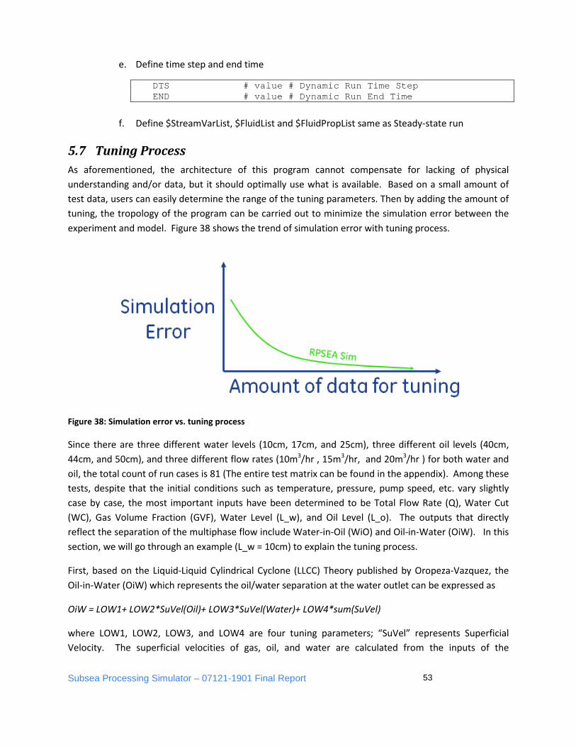
Subsea Processing Simulator – 07121-1901 Final Report 53
e. Define time step and end time
DTS # value # Dynamic Run Time Step END # value # Dynamic Run End Time
f. Define $StreamVarList, $FluidList and $FluidPropList same as Steady-state run
5.7 Tuning Process As aforementioned, the architecture of this program cannot compensate for lacking of physical understanding and/or data, but it should optimally use what is available. Based on a small amount of test data, users can easily determine the range of the tuning parameters. Then by adding the amount of tuning, the tropology of the program can be carried out to minimize the simulation error between the experiment and model. Figure 38 shows the trend of simulation error with tuning process.
Figure 38: Simulation error vs. tuning process
Since there are three different water levels (10cm, 17cm, and 25cm), three different oil levels (40cm, 44cm, and 50cm), and three different flow rates (10m3/hr , 15m3/hr, and 20m3/hr ) for both water and oil, the total count of run cases is 81 (The entire test matrix can be found in the appendix). Among these tests, despite that the initial conditions such as temperature, pressure, pump speed, etc. vary slightly case by case, the most important inputs have been determined to be Total Flow Rate (Q), Water Cut (WC), Gas Volume Fraction (GVF), Water Level (L_w), and Oil Level (L_o). The outputs that directly reflect the separation of the multiphase flow include Water-in-Oil (WiO) and Oil-in-Water (OiW). In this section, we will go through an example (L_w = 10cm) to explain the tuning process.
First, based on the Liquid-Liquid Cylindrical Cyclone (LLCC) Theory published by Oropeza-Vazquez, the Oil-in-Water (OiW) which represents the oil/water separation at the water outlet can be expressed as
OiW = LOW1+ LOW2*SuVel(Oil)+ LOW3*SuVel(Water)+ LOW4*sum(SuVel)
where LOW1, LOW2, LOW3, and LOW4 are four tuning parameters; “SuVel” represents Superficial Velocity. The superficial velocities of gas, oil, and water are calculated from the inputs of the
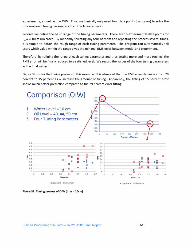
Subsea Processing Simulator – 07121-1901 Final Report 54
experiments, as well as the OiW. Thus, we basically only need four data points (run cases) to solve the four unknown tuning parameters from this linear equation.
Second, we define the basic range of the tuning parameters. There are 16 experimental data points for L_w = 10cm run cases. By randomly selecting any four of them and repeating the process several times, it is simple to obtain the rough range of each tuning parameter. The program can automatically tell users which value within the range gives the minimal RMS error between model and experiment.
Therefore, by refining the range of each tuning parameter and thus getting more and more tunings, the RMS error will be finally reduced to a satisfied level. We record the values of the four tuning parameters as the final values.
Figure 39 shows the tuning process of this example. It is observed that the RMS error decreases from 29 percent to 15 percent as w increase the amount of tuning. Apparently, the fitting of 15 percent error shows much better prediction compared to the 29 percent error fitting.
Figure 39: Tuning process of OiW (L_w = 10cm)

Subsea Processing Simulator – 07121-1901 Final Report 55
5.8 Simulation Results Figure 40 shows the comparison between simulation and experimental data for the results of Oil in Water (OiW). It is seen that the predicted results match the experiment very well. The RMS error increases as reducing the water level. When there is a higher water level in the separator, the values of OiW among these run cases are almost zero, which means only a small amount of oil can flow out from the water outlet.
Figure 40: Comparison between simulation and experiment (OiW, Steady-state runs) with RMS error shown as a percentage
Figure 41 shows the experimental data of WiO along with the results predicted by the program. As can be observed, the agreement between experiment and model is very good. The greatest RMS error happens at L_w = 17cm and L_o = 44, 50cm due to some abnormal data points. It is also seen that, although higher water level gives better separation at the water outlet, it induces worse separation at the oil outlet, i.e., more water comes out of the oil outlet. In addition, WiO shows a much clearer trend compared to OiW. Figures 42 and 43 validate that the program has sufficient accuracy to predict the oil/water separation for steady-state cases.

Subsea Processing Simulator – 07121-1901 Final Report 56
Figure 26: Comparison between simulation and experiment (WiO, Steady-state runs) with RMS error shown as a percentage
Figure 42 shows the trends of four tuning parameters for OiW and three tuning parameters for WiO. The purpose of these maps is to help users to determine the values of tuning parameters at certain water level and oil levels. For instance, when L_w = 17cm and L_o = 40cm, the tuning parameters for predicting WiO are LWO1 = -4.1, LWO2 = 5.8, and LWO3 = -1.4.

Subsea Processing Simulator – 07121-1901 Final Report 57
Figure 42: Trends of tuning parameters
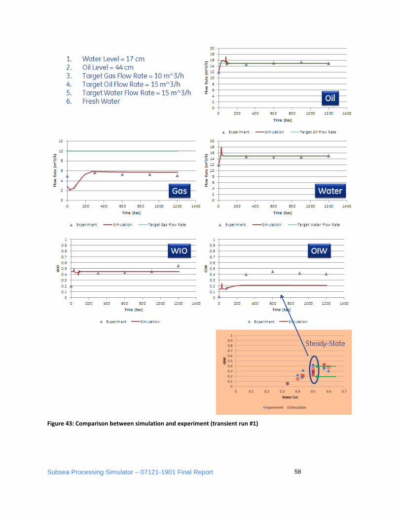
Subsea Processing Simulator – 07121-1901 Final Report 58
Figure 43: Comparison between simulation and experiment (transient run #1)

Subsea Processing Simulator – 07121-1901 Final Report 59
The experimental data versus model predictions comparison for data acquired under transient runs are presented in Figures 43 and 44. Water level, oil level, and the target flow rates of gas/oil/water for each transient run case are listed in the corresponding figure. The test data were recorded every five minutes until 20 minutes. It is observed that the time histories of gas flow rate, oil flow rate, and water flow rate match the experimental data very well. The same values of tuning parameters were used as steady-state runs. The comparison also reveals excellent agreement for WiO in both cases and OiW in case 2. The reason for the difference between experiment and simulation in OiW for case 1 is that this case exhibits the largest error in steady-state runs, shown as the right bottom plot. Since the same tuning parameters are employed, the transient run keeps the same level of error for this particular case.
Figure 27: Comparison between simulation and experiment (transient run #2)

Subsea Processing Simulator – 07121-1901 Final Report 60
5.9 Data Post-Processing In order to plot the Go/No-Go map that can help users to make the right decision, a specific surface fitting method has to be used since there are only limited experimental data points in Water Level vs. Oil Level plot. Thin Plate Spline regression (TPS) fits a thin plate spline surface to irregularly spaced data. The smoothing parameter is chosen by generalized cross-validation. A thin plate spline is result of minimizing the residual sum of squares subject to a constraint that the function has a certain level of smoothness (or roughness penalty). Roughness is quantified by the integral of squared m-th order derivatives. Besides controlling the order of the derivatives, the value of m also determines the base polynomial that is fit to the data. The degree of this polynomial is (m-1). In the program, the R function TPS() is used to realize the thin plate spline regression with the default setting. Figure 45 depicts OiW with respect to water level and oil level in a more straightforward way. When the water level is higher and the oil level is lower, we expect to see more WiO and less OiW. If we set the criteria for both WiO and OiW to “less than 25%”, the corresponding Go/No-Go maps are generated as Figure 46. By overlapping the maps of WiO and OiW, one can easily obtain a Go/No-Go map to satisfy the criteria of oil/water separation at both water outlet and oil outlet. For example, when the water level is set to be 19cm and oil level is set at 48cm, both WiO and OiW are less than 25 percent and provide approving separation. In this example the zones of compliance to the performance target appear as separate islands. If one of the specifications were to be considered more important than the other, aiming for the corresponding side of the island would ensure compliance with that requirement. If the simulations were to be repeated at different water cuts for the same total liquid flow rate, similar levels would result in different residence times for the oil and the water, and thus different boundaries for the water-in-oil and oil-in-water performance.
Figure 45: WiO and OiW maps in Oil level-Water level plane
10% 20% 25% 30%
40%
50%
0%
30% 25% 20% 10%

Subsea Processing Simulator – 07121-1901 Final Report 61
Figure 46: Go/No-Go maps for WiO and OiW (Criteria: <25%) shown as 2D maps above and 3D maps below.
6 Conclusions An architectural model was developed on which subsea processing simulations can be developed. It is a general purpose process Simulator featuring minimal architectural overhead that puts all the functionality in user developed unit models. The underlying goal is to remove all unnecessary impediments to allow the user full modeling license. Hierarchical modeling is enabled by standardized unit model interfaces, arbitrarily expandable data structures, tag-based calls, and an organization that aids, if not enforces, documentation. NPSS was used as the framework for the Simulator architecture. A
Subsea Processing Simulator – 07121-1901 Final Report 62
MATLAB version was developed as a bottom up tool to help drive the development. The Simulator has the capability to interface with commercial codes such as AspenTech’s HYSYS.
A flow loop with a three-phase separator was developed as a vehicle for validation. A model of the loop was built with the Simulator, a test matrix was simulated, and the tuning process was used to match data to simulation.
6.1 Future work With an architecture that is a viable framework to simulate subsea processing, the two logical next steps are to tackle a process that more closely simulates desirable produced flow management requirements in the GOM, and to simulate fluids that come closer to real produced fluids. In modeling these processes, it is suggested that physics such as surface tension due to pressure changes or more complex physical models for the gravity separation be considered (i.e., considering droplet packing, foam formation, film drainage, etc.).
6.2 Technology Transfer Technology transfer will be accomplished as follows. AspenTech will take over and maintain the Simulator. The unit models used to model the test flow loop have been translated into Aspentech’s Aspen Custom Modeler language and will be included in AspenTech’s Knowledge Database. This will make the Simulator available to anyone with a license to AspenTech’s suite of software tools. Through its consulting services AspenTech is available to assist users in the development of further system models and unit models.

Subsea Processing Simulator – 07121-1901 Final Report 63
Appendices
A. M ATLAB Simulator Tutorial
All simulator and model files used below are in this zip file:
A.1 A control valve Let’s kick the tires and model something—a control valve. The control valve will have liquid entering it at some flow rate and pressure. The valve model will then calculate the pressure drop incurred across the valve as a function of how far open the control valve is.
A.1.1 Control File
Let us start with a blank control file attached: Control_BLANK.txt and start defining things. After the comment symbol “%” on the first line let’s add a description of what this model will be. Let’s define two unit models by listing them in the $UnitList block after the comments but before the next block delimiter ($):
Tutorial_Upstream_1 # 1 # 1 # Upstream # Model that sets up upstream boundary conditions Valve_1 # 1 # 1 # Valve # easy valve model.
No blank lines are allowed within blocks. Note that the block comments guide the entry format. The text before the first # delimiter is the tag for that model. Appended to “model_,” it is also the m-file and function name. The second text is the Instance number. We can re-use the same models, and each can have its own parameters if so endowed. The third integer is the number of outlets contained in this unit model. The total number of outlets defines one of the dimensions of the stream and fluid data sub-structures. The Long Name is useful as the plotting tool can automatically use this string for legends; otherwise, it will use the model name which may be cryptic.
Next we can connect the two top-level unit models. This is done by adding the following line in the Connectivity block:
Tutorial_Upstream_1 # 1 # 1 # Valve_1 # 1 # Upstream BC to Valve.
As suggested in the Connectivity block comments, this line says “Outlet number 1 of the Tutorial_Upstream_1 model instance number 1 is connected to Instance 1 of the Valve_1 model.” This is not the only way to make connections, it is just convenient. We might also package the output of Tutorial_Upstream_1 in the Global array and tell Valve_1 where to find it. This will be important because unit models often communicate beyond neighbors. Brain Teaser: How does one handle reverse flow??? There are at least three distinct methods, left for now as an exercise.

Subsea Processing Simulator – 07121-1901 Final Report 64
Now we need to define our variables. Necessary information includes a flow rate, upstream pressure, valve setting, and flow rate going out. A fluid density will also be required. After the $GB.Data block comments and before the %%% Procedural … line, add the following:
Flow0 # 100 # [gpm] Q # Initial Flow Rate Pressure0 # 100 # [psi] P # Upstream Pressure Density # 997 # [kg/m^3] Water Density
Likewise in the $GlobalVarList block:
Cv # 5 # [gpm/sqrt(psi)] Valve flow Coefficient # This characterizes the valve
And in the $StreamVarList:
Pressure # i # [psi] Pressure Flow # e # [gpm] Flow Rate
Note that I document the units. Declaring variables automatically gives me a look-up table of sorts. Also, this is a steady state simulation, but I put Cv in the Global Block so I can store its time history during transient runs to be done later. For the Stream Variables, I set a code for whether each property is intensive or extensive (or I can define other codes—they will only be used if I write a unit model that uses them. Finally, if I were doing multiphase modeling, I would define a fluid (water) and a fluid property (Flow), and perhaps density, so that I could add different fluids and track their properties in this sub-structure instead of putting them in the Stream Variables list. But for now this will suffice.
Finally let’s look at the $SolverScript block. I only have two top level unit models and they are ordered sequentially, so if I leave SolverOrder commented out it will execute them 1-2. I don’t need iterations, so Single=True is fine. I do not need the structures prepared for another time step or batch run, so I will set NoAdvance=true. The last line, Tool_RunCase.m, will execute my instructions. If I had a more complicated network of models, I could break it down into subsets and execute the models optimally.
The Control File is now set and looks like this: Tutorial_Valve_1.txt
A.1.2 Unit Models
Now we owe the Simulator a couple Unit Models. Starting with a template model_BLANK.m we will save it as model_Tutorial_Upstream_1.m to be consistent with what we specified in the Control File. The first line needs to be modified to have the correct name:
function [Global, Stream, GB] = model_Tutorial_Upstream_1(Global, Stream, Unit, GB, INs, OUTs, Instance) Note that the function gets and returns the data structures. It also is given INs, which points to streams entering the model, and OUTs points to streams leaving the model which came from the connectivity block. It also knows what Instance it is.

Subsea Processing Simulator – 07121-1901 Final Report 65
Documentation: I comment on what this model does and copy in the lines from the Control File that this model needs for inputs and outputs - not needed but highly recommended. The block of code to pass stream/fluid data from inlet(s) to outlet(s) is not needed as this is the upstream block, but I’ll leave it.
Now for the model code:
Stream.Data(OUTs(1),Stream.ID.Pressure,end)=GB.Data.Pressure0; %[psi] Stream.Data(OUTs(1),Stream.ID.Flow,end)=GB.Data.Flow0; %[gpm]
That’s it. It is a lot of unit model text for such a small amount of actual executed code, but documenting what is in the models is as important as what is in the models. Note that the calls from the data structures are long, but self documenting. You can tell what it is doing even though I haven’t yet presented how the data structures are set up. This I will do now:
• GB data is called by GB.Data.<GB Name>, where ‘GB Name’ is the tag given in the control file.
• Global data is called as Global.Data(Global.ID.<Global Name>, end), where end signifies the current time step workspace. If solving iterative solutions, be sure to use end-1 as appropriate and note that the code may need to be skipped on the very first time step.
• Stream data is called as Stream.Data(<Location>,Stream.ID.<Stream Name>,end). <Location> can be from INs or OUTs as demonstrated. To connect somewhere else it looks like Unit.OutID.<Unit Name>_<Instance>(<outlet number>), which is unwieldy but necessary. I generally don’t have to do this because if these quantities are this important, I dump them to a Global Array, which is easy for picking up as well as plotting.
• Fluid data is at Stream.Fluid.Data(<Location>,Stream.Fluid.ID.<Fluid Name>,Stream.Fluid.PropID.<Fluid Property Name>,end)
The upstream model version 1 is now done: model_Tutorial_Upstream_1.m
Now for the valve model. We use the same steps above, and the actual model can look like:
Cv=Global.Data(Global.ID.Cv,end); %[gpm/sqrt(psia)] Specific_Gravity=GB.Data.Density/1000; %[] Q=Stream.Data(INs(1),Stream.ID.Flow,end); %[gpm] DP=(Q/Cv)^2*Specific_Gravity; %[psi] Pressure drop across valve Stream.Data(OUTs(1),Stream.ID.Pressure,end)=Stream.Data(INs(1),Stream.ID.Pressure,end)-DP; %[psi]
The first three lines gather the data, the DP line calculates, and the last line returns the result. Note the flow out of the valve was not need to be explicitly specified. It was passed from inlet to outlet earlier.
model_Valve_1.m

Subsea Processing Simulator – 07121-1901 Final Report 66
A.1.3 Run File
Starting with Main_BLANK.m , I update the path (cd …) and name of the control file (fname) or comment them out to get a GUI. I have nothing to plot, so I change “if true” to “if false”. I am interested in the pressure out, which I obtain with:
Stream.Data(Unit.OutID.Valve_1_1(1),Stream.ID.Pressure,end)
I save the file as Main_Tutorial_Valve1.m , which I can then execute. I get negative pressure which makes me realize I should go back and specify my units better (gauge or absolute pressure?). I can drop the flow rate or open the valve more (increase Cv) in the Control File to make the outlet pressure positive.
After executing the simulation, it is useful to look at the Data Structures to see how they are set up as the structures themselves are often a convenient place to check models and simulations.
A.2 Time for a Transient Run Let’s add a PID control, which will receive a measurement (downstream pressure), compare it to a set point, and output a command (control valve Cv) in an attempt to minimize error. I already have a PID controller model, so we will make a new Valve model that incorporates it as a sub-model. Then we will upgrade the upstream unit model to set up transient boundary conditions and run the simulation.
A.2.1 Valve Upgrade
The PID model I will use looks like this: model_PID1.m . Looking at this model, I can examine the actual code, but if I trust the model and it is well documented, I don’t need to do so. All I need to know is the variables it needs, which are documented at the head of the model, and make the connections and call in the host unit model.
I make a new version of my Control File: Tutorial_Valve_2.txt and add the lines needed to declare the new variables to the $GB.Data block. These are the “hooks” to connect my valve to the PID controller. I set initial values to “0” or some other number. Note that this PID model has bonus features such as a manual / PID control switch and limits, some of which we will hardwire in the valve model.
Now we will modify and save our valve model as a new version (model_Valve_2.m), add the PID controller, and update the documentation. The call to the PID controller is lengthy but explicit, which is useful for checking and documentation. Note that the PID_Com is a sub-model input and output. The
resulting value for Cv is stored in the Global sub-structure previously defined model_Valve_2.m .
Likewise, the upstream unit model will be updated to facilitate time evolving upstream conditions ,namely pressure and flow. As demonstrated, it uses linear interpolation with vectors to describe
pressure and flow at certain times model_Tutorial_Upstream_2.m .

Subsea Processing Simulator – 07121-1901 Final Report 67
Back in the control file, the $UnitList and $Connectivity blocks are updated with the new model names. All new variables are defined and the old upstream condition variables are removed. The $SolverScript needs to have NoAdvance set to “false” since this is a transient run, but there is still no iteration of unit
model execution required within a time step Tutorial_Valve_2.txt .
The Control File can hold the vectors to define the upstream pressure and flow history, but I have chosen to do so in the Run File, which is also updated to make the relevant plots:
model_Tutorial_Upstream_2.m
The simulation is executed using this last file.