rrr-robot : design of an industrial-like test facility for ... · rrr-robot : design of an...

RRR-robot : design of an industrial-like test facility fornonlinear robot controlvan Beek, A.M.

Published: 01/01/1998

Document VersionPublisher’s PDF, also known as Version of Record (includes final page, issue and volume numbers)

Please check the document version of this publication:

• A submitted manuscript is the author's version of the article upon submission and before peer-review. There can be important differencesbetween the submitted version and the official published version of record. People interested in the research are advised to contact theauthor for the final version of the publication, or visit the DOI to the publisher's website.• The final author version and the galley proof are versions of the publication after peer review.• The final published version features the final layout of the paper including the volume, issue and page numbers.

Link to publication

Citation for published version (APA):van Beek, A. M. (1998). RRR-robot : design of an industrial-like test facility for nonlinear robot controlEindhoven: Eindhoven University of Technology

General rightsCopyright and moral rights for the publications made accessible in the public portal are retained by the authors and/or other copyright ownersand it is a condition of accessing publications that users recognise and abide by the legal requirements associated with these rights.

• Users may download and print one copy of any publication from the public portal for the purpose of private study or research. • You may not further distribute the material or use it for any profit-making activity or commercial gain • You may freely distribute the URL identifying the publication in the public portal ?

Take down policyIf you believe that this document breaches copyright please contact us providing details, and we will remove access to the work immediatelyand investigate your claim.

Download date: 15. Nov. 2018

https://research.tue.nl/en/publications/rrrrobot--design-of-an-industriallike-test-facility-for-nonlinear-robot-control(44492a56-bd91-43ed-922e-6a88113c3446).html

RRR-robot :Design of an industrial-like testfacility for nonlinear robot control

ir. A .M. van Beek

Supervisors: Prof. dr. ir . J .J . Kokdr. ir . A .G. de Jagerir. L . Koddeir. J.P.A . Banens

Eindhoven University of Technology (TUE)Faculty of Mechanical EngineeringDivision of Fundamental Mechanical EngineeringSection Systems & ControlMay 1998WFW rapport 98.014

ISBN-GEGEVENS

A .M . van Beek'RRR-robot : Design of an industrial-like test facilityfor nonlinear robot control' / Beek, A .M. van ;- Eindhoven: Stan Ackermans Instituut . -Ill .Ontwerpers opl . Computational MechanicsMet lit . opg .ISBN 90-5282-858-XTrefw . : Robot-design / Robot control /

Summary

Improving performance In industrial robots, several (non)linear effects may reduce theperformance: configuration dependent inertia and conservative terms, Coriolis and centrifugaltorques, friction, flexibilities in joints and/or links, backlash, motor dynamics, and sensor dy-namics. By counteracting these unwanted effects, manipulators can become faster and/or moreaccurate. Various control schemes have been developed to deal with one or more of the nonlineareffects. For high-speed tracking of complex trajectories, the Coriolis and centrifugal torques forman essential part of the occurring nonlinear effects . Therefore, these terms play an importantrole in many of the proposed control strategies .

Experimental validation The RRR-robot (3 x Rotation) has been designed and build tofacilitate further development, i .e., to test and compare these concepts in an experimental setupwith a complexity comparable to industrial manipulators with multiple degrees of freedom . Toachieve a resemblance with conventional industrial robots (e .g., Puma-type robots), the systemhas a chain structure and three rotational degrees of freedom .

RRR-robot The main feature of this experimental facility is the ability to enhance the Coriolisand centrifugal torques relative to other nonlinear effects . This was achieved by eliminating twolimitations of conventional robots . First, sliprings were applied to realize unconstrained rotationof all joints . Thus enabling a combination of low accelerations (low inertia), and large velocities(large Coriolis and centrifugal torques) . Second, direct-drive servos (without transmissions) wereused to reduce the influence of motor inertia originating from gear boxes with high reductionratios, and to eliminate transmissions as a source of additional friction, backlash, and elasticity .

Another feature of the RRR-robot is a modular setup, i.e., the last link can be replaced bya flexible link, and the last joint can be transformed into a flexible joint . This makes it suitableto evaluate control schemes for both rigid-robots and flexible joint and/or link robots .

To control the robot, and to evaluate its performance, a PC based control system was selected .This system facilitates "rapid prototyping" . Control algorithms can be implemented by means ofgraphical block scheme manipulations where the resulting diagram is used to generate real-timecode .

Contents

Summary

1 Introduction 1

2 Design specifications 32.1 Problem formulation . . . . . . . . . . . . . . . . . . . . . . . . . . . . . . . . . . 32.2 Problem analysis . . . . . . . . . . . . . . . . . . . . . . . . . . . . . . . . . . . . 32 .3 RRR-robot specifications . . . . . . . . . . . . . . . . . . . . . . . . . . . . . . . 6

3 RRR-robot subsystems 93.1 Subsystems . . . . . . . . . . . . . . . . . . . . . . . . . . . . . . . . . . . . . . . 9

3.1 .1 Interactions . . . . . . . . . . . . . . . . . . . . . . . . . . . . . . . . . . . 103.1 .2 Design strategy . . . . . . . . . . . . . . . . . . . . . . . . . . . . . . . . . 10

3.2 Joint-Actuation System . . . . . . . . . . . . . . . . . . . . . . . . . . . . . . . . 113.2.1 Transmissions . . . . . . . . . . . . . . . . . . . . . . . . . . . . . . . . . . 113.2.2 Servo motors . . . . . . . . . . . . . . . . . . . . . . . . . . . . . . . . . . 113.2.3 Servo sizing . . . . . . . . . . . . . . . . . . . . . . . . . . . . . . . . . . . 14

3.3 Measurement System . . . . . . . . . . . . . . . . . . . . . . . . . . . . . . . . . . 173.3 .1 Joint-angle sensors . . . . . . . . . . . . . . . . . . . . . . . . . . . . . . . 173.3 .2 Link sensors . . . . . . . . . . . . . . . . . . . . . . . . . . . . . . . . . . . 193.3.3 Cartesian position end-effector . . . . . . . . . . . . . . . . . . . . . . . . 20

3.4 Control System . . . . . . . . . . . . . . . . . . . . . . . . . . . . . . . . . . . . . 223.4.1 Control implementation . . . . . . . . . . . . . . . . . . . . . . . . . . . . 223.4.2 Safety provisions . . . . . . . . . . . . . . . . . . . . . . . . . . . . . . . . 26

3.5 Signal-1Yansfer System . . . . . . . . . . . . . . . . . . . . . . . . . . . . . . . . . 27

4 Synthesis of subsystems 334.1 Manipulator frame . . . . . . . . . . . . . . . . . . . . . . . . . . . . . . . . . . . 33

4.1.1 Motor load . . . . . . . . . . . . . . . . . . . . . . . . . . . . . . . . . . . 334.1.2 Sliprings . . . . . . . . . . . . . . . . . . . . . . . . . . . . . . . . . . . . . 374.1.3 Eigenfrequencies . . . . . . . . . . . . . . . . . . . . . . . . . . . . . . . . 37

4.2 Measurement System: Cartesian measurement system . . . . . . . . . . . . . . . 374.3 Evaluation . . . . . . . . . . . . . . . . . . . . . . . . . . . . . . . . . . . . . . . . 38

4.3.1 Real-time performance . . . . . . . . . . . . . . . . . . . . . . . . . . . . . 384.3.2 Servo performance . . . . . . . . . . . . . . . . . . . . . . . . . . . . . . . 404.3.3 Design specifications . . . . . . . . . . . . . . . . . . . . . . . . . . . . . . 424.3 .4 Design goals . . . . . . . . . . . . . . . . . . . . . . . . . . . . . . . . . . . .43

- v -

5 Conclusions and recommendations 455.1 Conclusions . . . . . . . . . . . . . . . . . . . . . . . . . . . . . . . . . . . . . . . 455.2 Recommendations . . . . . . . . . . . . . . . . . . . . . . . . . . . . . . . . . . . 46

A Modeling the RRR-robot 47A.1 Introduction . . . . . . . . . . . . . . . . . . . . . . . . . . . . . . . . . . . . . . . 47A.2 Rigid manipulator model . . . . . . . . . . . . . . . . . . . . . . . . . . . . . . . 47

A.2.1 Direct kinematics . . . . . . . . . . . . . . . . . . . . . . . . . . . . . . . . 47A. 2. 2 Dynamics . . . . . . . . . . . . . . . . . . . . . . . . . . . . . . . . . . . . 49A.2.3 Inertia parameters . . . . . . . . . . . . . . . . . . . . . . . . . . . . . . . 51

A.3 Flexible model . . . . . . . . . . . . . . . . . . . . . . . . . . . . . . . . . . . . . 51A.3.1 Flexible-arm kinematics . . . . . . . . . . . . . . . . . . . . . . . . . . . . 52

A.4 Implementation . . . . . . . . . . . . . . . . . . . . . . . . . . . . . . . . . . . . . 52

B RRR-robot components 55B.1 Dynaserv servos . . . . . . . . . . . . . . . . . . . . . . . . . . . . . . . . . . . . . 55B .2 MultiQ plug-in and terminal board . . . . . . . . . . . . . . . . . . . . . . . . . . 56B.3 Sliprings . . . . . . . . . . . . . . . . . . . . . . . . . . . . . . . . . . . . . . . . . 57

13.3 .1 Power sliprings . . . . . . . . . . . . . . . . . . . . . . . . . . . . . . . . . 57B.3 .2 Signal sliprings . . . . . . . . . . . . . . . . . . . . . . . . . . . . . . . . . 58

C Budget (in Dutch) 59

D Time schedule 61

E Terminology 63

Bibliography 67

Chapter 1

Introduction

Industrial robots Robots' are applied in a great variety of fields, of which industrial auto-mated manufacturing is the most important one. Objectives such as reducing the manufacturingcosts, increasing the productivity, and improving (or maintaining) the product quality standards,represent the main factors that have promoted an increasing use of robotics technology. Nowa-days, typical robot applications include : materials handling (e .g., palletizing or packaging),manipulation (e.g., arc welding or spray painting), and measurement (e .g., object inspection) .

Not surprisingly, there is an increasing demand from industry for systems which can achievethese tasks faster and/or more accurately. If the increase of performance can be achieved at thesame price, both improvements will result in lower price per product since increased accuracymay result in a reduction of post processing steps, and the increase of velocity obviously increasesthroughput .

In order to achieve fast response times in combination with an acceptable effort (i .e., drivingtorque2), industrial manipulators should be lightweight constructions . However, lightweightrobot arms are also flexible. Especially at high velocities, deformations and vibrations can occurin both the joints and the manipulator's links . These unwanted dynamics seriously reduce arobot's accuracy. In applications which require precise tracking of a moving position reference,such as arc welding, laser cutting or gluing, this is a serious problem .

One way to avoid such unwanted dynamics is realizing a stiff construction, i .e ., stiff joints andstiff arms . Designing both stiff and lightweight manipulators, though, is a difficult engineeringtask .

Stiff behavior by control An alternate approach is letting the construction "behave stiffly"by using advanced control strategies to deal with the flexibilities in manipulator joints and/orlinks. Unlike conventional control designs, these strategies do not assume stiff and rigid behaviorbut are based on models describing the flexible components . For fast industrial robots, velocitydependent torques - like Coriolis and centrifugal torques - are expected to play a decisive rolein these models .

Due to rapid developments in computing hardware, the application of more complex andnonlinear control algorithms has become a viable option. However, implementations of controlstrategies based on flexible models are still rare in industrial robots [43] .

'According to the definition of the Robot Institute of America, a robot is a reprogrammable multifunctaonalmanipulator designed to move materials, parts, tools or specialized devices through variable programmed motionsfor the performance of a variety of tasks .

2The term "torque" is used in a general sense, and denotes both torques and forces .

- 1 -

2 Introduction

Objective RRR-robot The main objective of the RRR-robot3 design project, is to realizea manipulator-like system to test these advanced nonlinear control strategies . To achieve aresemblance with conventional industrial robots (e .g., Puma-type robots), the system shouldhave a chain structure and at least three rotational degrees of freedom .

Although several other nonlinear effects (e .g., friction) may also reduce the performance, inthis project the focus is on highlighting the Coriolis and centrifugal torques . Therefore, themain requirement of the robot is the ability to maintain these torques at a significant level .

The project is financed by the Eindhoven University of Technology (EUT) in the contextof the participation in the Dutch Institute for Systems and Control (DISC) . One of its goals isto tighten the bonds between the various research groups which constitute the research schoolDISC. Therefore, the project involves an array of input from Mechanical Engineering, ElectricalEngineering, and Control Engineering .

Outline of this report In Chapter 2, the problem which the RRR-robot aims to solve isanalyzed, and all relevant design specifications are summarized . Next, in Chapter 3, the robotis conceptually divided into four subsystem : a Joint-Actuation System, a Measurement System,a Control System, and a Signal-Transfer System . Each of these subsystems is discussed indetail, and working solutions, or even components are chosen . In Chapter 4, the chosen workingprinciples are combined to form a complete system, and the design specifications are evaluated .Finally, in Chapter 5, some conclusions are presented and recommendations are made for futurework .

In the Appendices, technical details and additional information are gathered . The used rigid-robot model is discussed in Appendix A . In Appendix B, the RRR-robot components and theirmain features are listed . The budget and time schedule regarding the design and constructionare presented in Appendix C and D . In Appendix E, the used terminology is summarized .

Detailed information with regard to the use and assembly of the robot is presented in theRRR-robot instruction manual [41] . For a survey on 3D measurement systems for robot manip-ulators see [40] .

3The triple R stands for three rotational degrees of freedom .

Chapter 2

Design specifications

The main problem in evaluating (non)linear control laws designed for high speedtracking is to separate Coriolis and centrifugal torques from other nonlinear effects .In this Chapter, it is explained why this evaluation requires a new experimentalfacility. By analyzing the problem and thus exploring the main requirement, twoimportant features of the RRR-robot are identified . Finally, all the RRR-robotspecifications are summarized .

2.1 Problem formulation

In any (industrial) manipulator, several (non)linear effects may reduce the performance : con-figuration dependent inertia and conservative terms, Coriolis and centrifugal torques, friction,flexibilities in joints and/or links, backlash, motor dynamics, and sensor dynamics . Variouscontrol schemes have been developed to deal with one or more of these effects .

For high-speed tracking of complex trajectories, the Coriolis and centrifugal torques form anessential part of the occurring nonlinear effects . Therefore, these terms play an important rolein many of the proposed control strategies [12, 23, 24] . For further development it is necessaryto test and compare these concepts in an experimental setup with a complexity comparable toindustrial manipulators with multiple degrees of freedom [5] .

Problem statement The main problem is to enhance the Coriolis and centrifugal torquesrelative to other linear and nonlinear effects . In an industrial manipulator these effects mayobscure the influence of the velocity dependent torques . The objective of the RRR-robot isto solve this problem, i .e., to highlight the influence of Coriolis and centrifugal torques in anexperimental facility with an industrial-like complexity.

2.2 Problem analysis

Maintaining the Coriolis and centrifugal torques at a significant level during a considerableperiod meets with two fundamental limitations in most existing manipulators :

. the rotation of each joint is constrained to a certain angle due to the cables used for energyand data transport throughout the manipulator ;

4 Design specifications

• the presence of gears with high transmission reduction ratios (e .g. harmonic drives) tendsto linearize the system dynamics . Furthermore, gear boxes are a source of additionalfriction, backlash and elasticity .

To illustrate these limitations, consider a simple rigid manipulator model' (rigid joints andlinks). Without flexibility, friction, backlash, motor dynamics or, sensor dynamics, the equationsof motion are given by

M(q) 4 + C(q , 4) q+ g(q) = T (2.1)

where q denotes the vector with rotation angles, q the angular velocities, and q the angularaccelerations . So the torques T acting on each link consist of inertia terms, M(q) q , Coriolis andcentrifugal torques, C(q, q) q, and conservative torques due to gravity g (q) .

Constrained rotations In order to highlight the Coriolis and centrifugal torques for any linki, the contribution {C(q , q ) q}2 should be "substantial" during a "sufficiently" long period oftime. To quantify this requirement, the following ratio is defined :

fo I{C(g , g) g}2 1 d~ (2.2 )00r__

fo I {M(q) q}i +{C(q, q) q}Z +{g (q)}Z I d~ .

Highlighting the Coriolis and centrifugal torques now means achieving a large ratio . As can beseen in (2 .1), this can be achieved by a combination of high velocities and low accelerations . Ifthe joint rotation angles are limited, such a combination can be achieved only with considerableenergy (using powerful, expensive servos) and only over a short period of time, since shortly afterthe acceleration to a certain velocity, the de-acceleration must begin in order to avoid breakingany cables. Furthermore, the large injection of energy will excite additional vibrational modes,thus clouding the contribution of the Coriolis and centrifugal torques .

Transmissions To understand the linearizing effect of transmissions, first, they must be in-cluded in the model. Assume the transmissions are rigid and without backlash . Let qm and r,,,,denote the vectors of joint actuator displacements and actuator driving torques respectively ; thetransmissions then establish the following relationships :

f q,, n = KT ql Tm = K,717

where K,, is a diagonal matrix containing the gear reduction ratios k,.i . The central moments ofinertia, I,.,Lt, of each motor with respect to its rotor axis are collected in the diagonal matrix h,,, .

The mass matrix M(q) can be split into a constant diagonal matrix, KrI7zKT and a configuration-dependent (dependent on functions of q) matrix OM(q), i.e .,

M(q) = KrImKr + OM(q) . (2 .4)

Substituting (2 .3) and (2.4) into (2.1) yields

?m,=Imq +d-m

'In Appendix A, the derivation of models for rigid robots is considered in more detail .

2.2 Problem analysis

where i

d = K,-' OM(q)Kr l qm + Kr -1 C( q, q) Kr -1 qm + Kr 1g (q)

q-Kr1qm

5

represents the contribution depending on the configuration. As illustrated by the block schemeof Fig . 2.1, the system described by (2 .1) actually consists of two subsystems :

I

Figure 2.1 : Block scheme of a rigid manipulator with transmissions .

• a linear and decoupled subsystem in which each component of T,, .t influences only thecorresponding component of qm, and

• a nonlinear and coupled subsystem .

In case of high reduction gears (k,.i » 1), the contribution of the nonlinear interaction term d issmall, and can be considered as a disturbance for each joint servo . As a result the ratio of (2 .2)becomes small, since the torque TZ is almost completely determined by the motor inertia .

The price to pay, however, is the occurrence of joint friction, elasticity, and backlash thatmay limit system performance more than the nonlinear terms (d in (2 .6)). The use of driveswithout transmissions, direct-drives (Kr = I), could eliminate these drawbacks, but the influenceof nonlinearities and coupling between the joints then becomes relevant . Aside from the costand size of this actuator type this is the main reason that these servos are not yet very popularin industrial manipulators [34] .

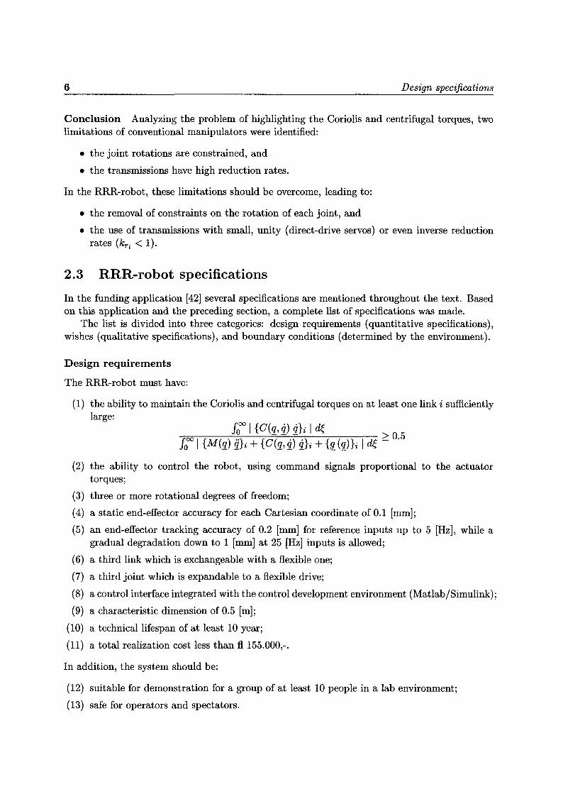
6 Design specifications

Conclusion Analyzing the problem of highlighting the Coriolis and centrifugal torques, twolimitations of conventional manipulators were identified :

• the joint rotations are constrained, and

• the transmissions have high reduction rates .

In the RRR-robot, these limitations should be overcome, leading to :

• the removal of constraints on the rotation of each joint, and

• the use of transmissions with small, unity (direct-drive servos) or even inverse reductionrates (kTro < 1) .

2.3 RRR-robot specifications

In the funding application [42] several specifications are mentioned throughout the text . Basedon this application and the preceding section, a complete list of specifications was made .

The list is divided into three categories : design requirements (quantitative specifications),wishes (qualitative specifications), and boundary conditions (determined by the environment) .

Design requirements

The RRR-robot must have :

(1) the ability to maintain the Coriolis and centrifugal torques on at least one link i sufficientlylarge :

f~ 1 {c(q , q) q}i 1 d~ > 0.5f°O 1 {M(q) q}i + {C(q, q) q}i + {g (q)}i 1 d~

_

(2) the ability to control the robot, using command signals proportional to the actuatortorques ;

(3) three or more rotational degrees of freedom ;

(4) a static end-effector accuracy for each Cartesian coordinate of 0 .1 [mm] ;

(5) an end-effector tracking accuracy of 0.2 [mm] for reference inputs up to 5 [Hz], while agradual degradation down to 1[mm] at 25 [Hz] inputs is allowed ;

(6) a third link which is exchangeable with a flexible one ;

(7) a third joint which is expandable to a flexible drive ;

(8) a control interface integrated with the control development environment (Matlab/Simulink) ;

(9) a characteristic dimension of 0.5 [m] ;

(10) a technical lifespan of at least 10 year ;

(11) a total realization cost less than fl 155 .000,- .

In addition, the system should be :

(12) suitable for demonstration for a group of at least 10 people in a lab environment ;

(13) safe for operators and spectators .

2.3 RRR-robot specifications 7

Compared to the funding application there are two significant omissions :

• maximal angular velocities of 1 x 27r, 5 x 21r and 25 x 21r (rad/s) for the first, second andthird link respectively ;

• maximal accelerations based on reaching the maximal velocities within one revolution orwithin 0.5 (s), whichever results in the largest acceleration .

Considering the objective, these requirements can be replaced by the more relevant require-ment (1), regarding torques instead of velocities and accelerations .

Design goals

If possible, the system should fulfill the following goals (in descending importance) :

(a) modern, state-of-the-art techniques should be applied ;

(b) future expansion (e .g. more sensors) should be possible ;

(c) a recognizable relation with industrial manipulators should exist ;

(d) maintenance should be easy ;

(e) insight into the robot's working principles should exist .

Boundary conditions

Finally, the RRR-robot project is subject to certain boundary conditions with respect to itsenvironment and users :

• the system will be operating in a laboratory environment ;

• within the research school DISC, the RRR-robot is to be used as a research object forseveral research groups .

Chapter 3

RRR-robot subsystems

In this chapter, the RRR-robot is conceptually divided into subsystems for jointactuation, measurement, control, and signal transfer. Each subsystem is discussed,and appropriate components or design solutions are chosen .

3.1 Subsystems

To tackle the design problem, a choice is made to conceptually divide the RRR-robot into severalsubsystem based on their function . To a certain extent, these subsystems can be consideredindependently. In the following, all subsystems, and their interactions are defined .

. The Joint-Actuation System consists of

- transmissions, and- servo motors with appropriate power supplies and power amplifiers .

• The Measurement System consists of

- joint sensors (e .g., to measure joint-angles),- link sensors (e .g., strain gauges), and- a 3D measurement system to determine the Cartesian position of the end-effector

independently from the joint sensors .

• The Control System consists of

- hardware components for data acquisition, command output, and overload protection ;- software components to implement the control algorithm, and user interface ; and- a hardware platform to execute the software .

Connections between these hardware components are also viewed as part of the ControlSystem .

. The Signal-Transfer System consists of components for the transport of

- power, and- measurement signals, across parts which move relative to each other .

10 RRR-robot subsystems

This includes transport between power amplifier and servo motor ; between MeasurementSystem and Control System; and between Control System and power amplifier . In somecases the Signal-Transfer System is reduced to a simple stationary connection (e .g., anelectric cable, or hydraulic duct) .

3.1.1 Interactions

In Fig. 3.1, a possible functional lay-out of the RRR-robot is shown .

% power

/measurement/control signals

i~ power power~ supplies amplifiersI

ControlSystem

Measurement Systemi

~ joint link Cartesian i~ sensors sensors position(s) i

-----------------, ( robotservo trans- ~ jointsmotors missions i and

_ ~ linksJóint-Xctuátióngystém

Signal-TransferSystem

I

Figure 3.1 : A possible functional lay-out of the RRR-robot's subsystems, and their interaction .Note that, especially the position of the Signal-Transfer System relative to the Joint-ActuationSystem may vary (e .g., depending on the type and placement of the power amplifier) .

The choice of the Joint-Actuation System determines the type of power transported bythe Signal-Transfer System, e.g., electrical, hydraulic or pneumatic . The Measurement System,together with the Joint-Actuation System, completely determines the requirements of the Signal-Transfer System, i .e., the amount and type of transport channels . The Control System mainlyinteracts with the Measurement System . It must be able to process measurements from allsensors. The interaction with the servos is restricted to three (usually electrical) commandsignals .

3 .1 .2 Design strategy

In designing the RRR-robot, each subsystem is considered separately, and an initial designsolution or component is chosen. Because of the interactions, the order in which the subsystemsare discussed is not unique .

The chosen starting point is the Joint-Actuation System since this determines the perfor-mance of the robot in terms of the design requirement (1) (Section 2 .3) .

Next the Measurement System and the Control System are addressed . These subsystemsare mainly interdependent . Any additional link sensors, but also the components of the 3D

3 . 2 Joint-Actuation System 11

measurement system which are attached to the end-effector can be considered as black boxeswith certain mass and (electrical) interface to the Signal-Transfer System .

Finally, the Signal-Transfer System is discussed based on the transport specifications imposedby the Joint-Actuation System and the sensors of the Measurement System . Obviously, this is aniterative procedure . If in any stage no satisfactory design solution can be found, it is necessaryto return one or more steps .

3.2 Joint-Actuation System

In the following sections, the components of the Joint-Actuation System are discussed . A choiceis made to use brushless DC motors as direct-drive servos (without transmissions) . Finally, arigid-robot model is used to aid servo sizing .

3.2 .1 Transmissions

Since servo motors typically provide high speeds with low torques, transmissions are often nec-essary to transform these quantities into the required opposite combination : low speeds withhigh torques. On the other hand, transmissions are also an important (additional) source ofjoint friction, elasticity, and backlash .

To eliminate these drawbacks, attempts have been made to develop actuation systems whichallow direct connection of the motor to the joint without the use of any transmission element .The use of such direct-drive actuation systems is not yet popular for industrial manipulators,mainly because of the control complexity; due to the absence of reduction gears, the nonlinearterms in the dynamic model can no longer be neglected (see section 2 .1) .

For the RRR-robot, however, this complexity is exactly what we want . Furthermore, theapplication of direct-drives also complies with the first design goal : modern state-of-the-arttechniques (design goal (a), Section 2.3)

Although the control complexity could be increased even more by using transmissions withinverse reduction rates (k,.i < 1), such "inverse transmissions" present several problems anddisadvantages. First of all there are technical problems finding appropriate, powerful enough,actuators to drive transmissions which reduce the output torque. Secondly, those transmissionhave all the disadvantages of "regular" transmissions : additional friction, elasticity and backlash(or, if not, are rather expensive) . Finally, with inverse reduction rates the relation with futureindustrial manipulators (design goal (c)) is lost .

3 .2.2 Servo motors

Motor types used for the actuation of joint motions can be classified into three groups :

1 . Pneumatic motors,

2 . Hydraulic motors, and

3 . Electrical motors .

Of this groups the following servos are typically used for direct-drive applications :

• hydraulic motors, and

• electrical motors :


- Variable Reluctance Stepper (VRS) motors,- Direct-Current (DC) motors, and- Brushless Direct-Current (BDC) motors .

Pneumatic motors are not suitable for applications where continuous motion control is of concerndue to their unavoidable air compressibility errors . They are mainly used in simple pick-and-place applications and for opening and closing motions of the jaws in a gripper tool .

Asynchronous induction motors are typically suited to deliver high power (> 1 kW) . Due tothe control complexity, they are not yet popular for servos .

Hydraulic motors Compared to electrical motors, hydraulic motors have several advantages .They:

• can achieve much higher torques at low velocities,

• have an excellent power-to-weight ratio, and

• are self-lubricated and self-cooled by the circulating fluid .

However, they also present the following drawbacks :

• need for a hydraulic power station,

• temperature dependent dynamics,

• need for regular maintenance, and

• pollution of the working environment due to oil leakage .

The last drawback is a significant problem, especially in combination with the specified uncon-strained rotation (from requirement (1)) in each joint . Since the hydraulic lines (conductingthe power signals) must pass through a signal transfer system with relative motion, leakage isdifficult to avoid .

Mainly because of this last problem, a choice was made to use electrical motors .

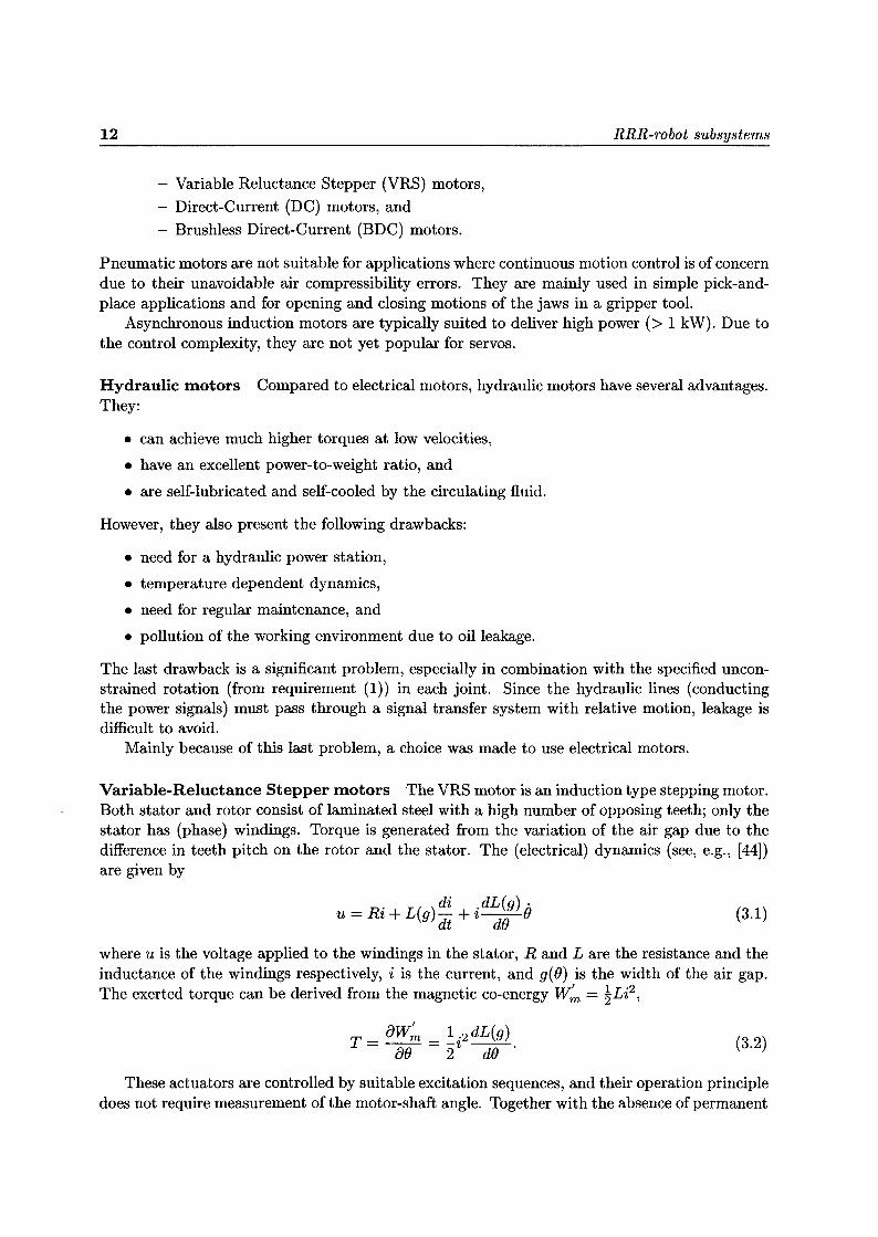
Variable-Reluctance Stepper motors The VRS motor is an induction type stepping motor .Both stator and rotor consist of laminated steel with a high number of opposing teeth ; only thestator has (phase) windings. Torque is generated from the variation of the air gap due to thedifference in teeth pitch on the rotor and the stator . The (electrical) dynamics (see, e.g., [44])are given by

u= Ri + L(g)át di + i d8dL(g) 6 (3.1)

where u is the voltage applied to the windings in the stator, R and L are the resistance and theinductance of the windings respectively, i is the current, and g(O) is the width of the air gap .The exerted torque can be derived from the magnetic co-energy Wm = 2Li2,

T _ aWr. _ 1i2 dL(g) (3.2)ae 2 d9

These actuators are controlled by suitable excitation sequences, and their operation principledoes not require measurement of the motor-shaft angle . Together with the absence of permanent

3.2 Joint-Actuation System 13

magnets, this results in simple and cheap actuators . However, the stepping nature of thismotor type restricts the position accuracy, causes vibrations, and introduces a significant torqueripple. Such inconveniences confine the use of stepper motors to applications, where low-costimplementation prevails over the need for accuracy and high dynamic performance .

With the use of a controller (and motor-shaft position feedback), the mentioned problemscan be partly solved ; torque control however, is difficult to realize .

Direct-Current motors Like the regular DC motor, the direct drive version consists of astator' which generates a permanent magnetic field (by ferromagnetic ceramics or rare earths),and a winded rotor which is powered via brushes and commutators .

The design goal of a direct-drive DC motor is to maximize output torque rather than power .The torque T is the product of the torque constant Kt and the rotor current i ;

T = Kt i . (3.3)

Since the torque constant is determined by the motor inductance L(Kt - L), two importantfeatures of direct-drive DC motors emerge [2] :

• a bulky or sometimes "pancake" like appearance because a large inductance requires aconsiderable motor volume (and mass) : L - l,.dT where lT and d,, are the rotor length andthe rotor diameter respectively ;

• a considerable electric time constant Te = R which is often no longer negligible .

Maximizing the current meets with an important limitation of the DC motor in general : me-chanical commutation . At the brush and commutator, large sparks can occur especially incombination with a large inductance . These sparks cause the brush to wear quickly and causeunwanted noise . Furthermore, the brush mechanism increases mechanical friction .

Note that the torque of (3 .3) is not constant due to the effect of the discrete commutation .The (maximum) deviation from the average torque is called the torque ripple .

Brushless Direct-Current torque motors In a brushless DC motor, mechanical commu-tation has been replaced with electronic commutation . Unlike conventional DC motors, therotor consists of permanent magnets, while the stator consists of several phase windings . Thecommutation of currents is accomplished by measuring the rotor position using a position sensor .

The elimination of brush and commutator allows an improvement of motor performance interms of higher torques and less material wear, and is therefore the main reason for using BDCmotors .

The inversion between the functions of stator and rotor leads to further advantages . Thepresence of a winding on the stator instead of the rotor, facilitates heat disposal . The absence ofa rotor winding allows construction of more compact rotors, which in turn have a lower momentof inertia. As a result, the size of a BDC motor is smaller than that of a regular DC motor ofthe same power .

The superiority of the brushless motor, though, comes at a cost : the rotor position must bedetected or measured, and fed back to the power amplifier (typically a DC-to-AC converter) .However, if such an internal sensor is accurate enough for robot control purposes, no additionaljoint position sensors are necessary, and the construction becomes more compact .

'Brushed DC motors come in a wide range of configurations, this configuration (permanent magnet stator andwinded rotor) is most common in direct drive applications [1] .


Conclusion Considering the obvious advantages of BDC motors, a choice is made to usebrushless direct-drive motors for all joints . Preferably, the internal sensors should be used forthe robot control .

3.2.3 Servo sizing

Choosing appropriate servos for the RRR-robot is an iterative problem, since, even for brushlessdirect-drive servos, the torque-to-mass ratio is small (see Fig . 3.2) . So, as a result of the requiredtorques, each motor has also a significant mass . To accelerate these masses, even larger motorsmay be necessary.

Torque v.s. Mass

102 0

Ez+

+

0

0

x

0

x

0

x

+ 0 Dynaserv BDC (<2 [rps])A Megatorque Stepper (<3 [rps])x SV BDC (<20 [rps])+ Mini RS BDC + harmonic drive 1 :50 (<1 [rps])

101Mass [kg]

102

Figure 3.2: Maximum torque versus mass for several commercial servo series : the Dynaservbrushless DC motors [26], the Megatorque stepper motors [29], the SV brushless DC motors [9],and the mini-RS BDC motors with integrated harmonic drive [17] . The first two are specificallydesigned for direct-drive applications .

To aid the motor choice, a rigid-manipulator model of the RRR-robot is used . The derivationof this model is described in Appendix A . The aim is to find three motors with the rightcombination of mass, torque and angular velocity ; at least one link should have a performanceratio r of 50 % or more at the largest possible angular velocity.

Based on an initial design sketch, a rough estimate was made for the link parameters (i .e.,dimensions and material) leading to the main system parameters shown in the upper partof Table 3.1. Because of its low mass density, aluminum is chosen as construction material .To illustrate this initial design, the kinematic relations (section A .2.1) were used to draw thesimplified wire-frame picture of Fig . 3 .3 .

3.2 Joint-Actuation System 15

Table 3.1 : Main system parameters used in evaluation model. The links are assumed to be hollowrectangular aluminum beams . The motor data are taken from the Dynaserv series of Litton PrecisionProducts .

parameters link/joint 1 2 3link length [m] 0.5 0.2 0.3link mass [kg] 9.86 1 .21 0.73motor mass [kg] 12 7.5 5.5motor inertia [kg m2] 0.023 0.015 0.012max. torque [Nm] 60 30 15

t= 0

t= 0.13

t= 0.065

t= 0.195

Figure 3.3: A wire-frame "animation" of the initial design . All quantities are in SI-units : t in[s], and x, y, z in [m} .

After choosing an appropriate motion pattern, i .e., with a high ratio r, a commercial motorcan be evaluated by substituting its mass and rotor inertia .

Selection

With the Dynaserv series of BDC motors of Litton Precision Products (see the motor data in thelower part of Table 3 .1) the main design requirement, maintaining high Coriolis and centrifugalforces, was met. This is illustrated in Fig . 3.4 with on the left the torques required to realizea stationary motion pattern (without inertia effects because qi = 0, so with large ratios ri)

HLtat =[ir t, 27r t, 37r t]T [rad] ; on the right are the torques required to realize a motion patternwith accelerations : qdYn = [sin ir/2 t, sin 37r/2 t, sin 37r t]T [rad] . Both motion patterns are chosen


to achieve the maximum torque of one or more motors .

Without accelerations

'ff 20Z_N 0w .O0~ -20

0

~ 5z~^ 0~0s2 -5

0

I

1time [s]

2

2

With accelerations

UW

Figure 3 .4: Required motor torques (thick black lines) to realize a chosen motion patternwithout accelerations (on the left) and with accelerations (on the right) . The contributionof the Coriolis and centrifugal torques is shown with a thick grey line .

Evaluation of (2.2) for each link yields r= [1, 0.39, 1] for qstat and r= [0.51, 0 .03, 0 .20] for

q_dYn . So for both motion patterns, the Coriolis and centrifugal component of motor 1 is abovethe required 50% of the total torque .

In addition, these servos can be used as complete self-contained joints with internal bearingsand sensors . Thus simplifying the design of the manipulator . In Section B .1, the main featuresand specifications are summarized .

Risk analysis

In their function of compact joint-units, the use of the selected Dynaserv servos involves a numberof potential risks; damage to the servos may occur due to thermal or mechanical overload .

. Thermal overload : due to heat development the allowed motor temperature (45 °C) isexceeded .Action: correspondence with the supplier guaranteeing that heat development in closedenvironments is not a problem (Litton 4-11-96) .

. Mechanical overload : the allowed static or dynamic moment load (see Table B .1) may beexceeded .Action: designing the manipulator frame based on minimizing the moment loads on theservos (see Chapter 4) .

3.3 Measurement System 17

3.3 Measurement System

In this Section, sensors are chosen for the measurement of the joint angles, and the Cartesianposition of the end-effector. Additional link sensors will be realized later, so they are discussedonly briefly with the emphasis on their possible interaction with the manipulator design (e .g .,mass) and other subsystems, such as the Signal-Transfer System and the Control System (e .g .,data transport and conditioning) .

3.3 .1 Joint-angle sensors

First the specifications for the static and tracking accuracy of the end-effector are translatedinto joint-angle specifications for each joint. After discussing two types of suitable sensors, achoice is made to use incremental encoders built-in with the motors .

Specifications

Assuming that the end-effector position is determined only by the joint angles q (see [36]), thesensitivity of the end-effector to variations Oqi is maximal when link 1 and 2 are perpendicularand link 2 and 3 are aligned (see Fig . 3.5) .

.Z12

q301

Figure 3.5: Sensor specifications

::;;Iz

In this configuration, the angles Oq2 and Oq3 both influence the position error in the z-direction. To simplify the design by using the same sensor for joint 2 and 3, both errors arechosen equal, i .e., Oq2 = Oq3 . Then the relation between the position error of the end-effector,e=[Ox, Ay, Oz]', the link length li, and the joint angle deviation Oqi is given by :

_ Ox _ AY~ql ~ 12 +13 1 2 +13 (3.4)

OzOqa Aqs

_

^- 12+213

With the specified static and tracking end-effector accuracy for each Cartesian coordinate (seeSection 2.3) and a first choice of the link length li the joint-angle specifications are given inTable 3.2 .

13


Table 3 .2 : Joint-angle specifications . The required bit resolution is determined by the staticerror. Note that, joint-angle sensor 2 and 3 have identical specifications because the allowableerrors aq2 and Oq3 (not their contributions to the end-effector error Oz) were chosen equal .

quantity link 1 link 2 link 3length li [m] 0.5 0.2 0.3static error Oqi < x 10-3 [rad] 0.20 0.125 0.125

[arc-sec] 41.3 25.8 25.8tracking error Oqi < x 10-3 [rad] 0.40-2.00 0.25-1 .25 0.25-1 .25(5-25 [Hz]) [arc-sec] 82.5-412 .5 51.6-257.8 51 .6-257.8required sensor resolution [bit] 15 16 16

Sensor types

The most common transducers used in robot applications are resolvers (or synchros) and (abso-lute or incremental) encoders because of their precision, robustness, and reliability . Both typeshave operating principles which enable an accuracy within the specifications (up to 20 [bit] forencoders, and up to 16 [bit] for resolvers) to . Other sensors to measure angular displacementare either not accurate enough to meet the required joint specifications (e .g., potentiometers,up to 10 [bit] resolution), or have accuracies well above these specifications (e .g., inductosyn, 18to 22 [bit]) [13] .

Resolver The operating principle of the resolver is based on the mutual induction betweentwo electric circuits which allow continuous transmission of angular position without mechanicallimits. From a construction viewpoint, the resolver is a small electric machine with a stator anda rotor fed by a sinusoidal voltage . The information on the angular position is associated withthe magnitude of the supply and induced sinusoidal voltages, which are treated by a suitableresolver-to-digital converter (RDC) to obtain the digital data corresponding to the positionmeasurement . In the process also analog velocity measurements become available .

Encoder An encoder consists of an optical-glass disk on which concentric tracks are madewith alternating transparent and opaque sectors . A light beam is emitted perpendicularly tothe disk; for each track a photodiode is used to determine whether a sector is transparent or not .In an absolute encoder the pattern of sectors is unique for each position on the disk . The numberof tracks determines the resolution of the encoder, e.g., a 12 [bit] absolute encoder requires 12tracks .

Simpler from a construction viewpoint (and thus cheaper) is the incremental encoder whichin its most basic form has only one track with equally distributed sectors . The absolute positionis determined by means of suitable counting and storing circuits . Often a second track is added todetermine the sign of the rotation and improve the resolution . To define an absolute mechanicalzero as reference, sometimes a third track with one opaque sector is added . Note that in contrastwith the absolute encoder, the position information is more sensitive to disturbances .

Velocity measurements can be reconstructed by using a voltage-to-frequency converter (withanalog output), or by (digitally) measuring the frequency of the pulse train .


Selection

Although 15 or even 16 [bit] absolute encoders exist, they are rare and extremely expensive .So two options remain : the resolver and the incremental encoder . By construction the resolvertype sensor with winded stator and rotor coils is heavier then the encoder with only an opticaldisk .

The chosen Dynaserv motor is available both with a resolver (DR-series : accuracy ±45[arc-sec]), or with an incremental encoder (DM-series : accuracy ±15 [arc-sec]) . Based on thejoint-angle specifications (Table 3 .2), a servo from the DM-series with an incremental encoderis selected for all three joints . Note that the DR-series servos also have a 30%-60% smallertorque-to-mass-ratio then the DM-series .

Risk analysis

The main risk using incremental encoders is the sensitivity for (electronic) disturbances . Everymissed pulse reduces the position accuracy. See Section 3 .5 for a more detailed discussion .

3.3.2 Link sensors

Several possible sensors to determine deflection or acceleration of the link are discussed withrespect to their interaction with the rest of the system .

Strain-gauge

Strain-gauges can be used to measure the local strain of a link . The most used type is thebonded metal-foil gauge . The strain, L is determined from the relative change in resistance ofthe metal conductor, i.e .,

dR/RdL/L =Gauge factor (3.5)

The Gauge factor depends on the material properties of the strain-Gauge and can not be mea-sured directly, but is determined by sample testing with a typical accuracy of ± 1 % .

To measure the deflection of a beam, a Wheatstone bridge with 4 strain-Gauges can be used .When using a battery for the supply voltage (0 .5-5 [V] with a typical gauge current of 5-40[mA]), two signal lines are needed for each deflection measurement . Since the output voltage isquite small (a few microvolts to a few millivolt) amplification is needed .

Any loading effect of the Signal-Transfer System can be counteracted by (regular) calibrationprovided the resistance of the supply lines changes only slowly in time . To improve the signal-to-noise ratio, the strain-gauge output should be amplified as early as possible .

Inertial sensors

Inertial measurement sensors such as gyroscopes and accelerometers measure rotation rate, andacceleration, respectively. The measurements can be integrated to obtain the change in orien-tation (yaw, pitch and roll) and double-integrated to determine the change in position (Ox,Dy,and Oz). In [40], the properties of several types of (commercial) accelerometers, and gyroscopesare addressed.

When used for tracking the position and/or orientation, inertial sensors have the advantagethat they consist of self-contained, small, and light (< 0 .5 [kg]) units . No receiver/transmitter


set-up is required . The possible update rate is limited only by sensor bandwidth . Anotheradvantage of these sensors is a basically unlimited range, independent of the tracking accuracy .However, integrating the data means that only relative orientation or position is measured ; aknown starting or reference point is required . Moreover, any constant error increases withoutbound after integration. Therefore, inertial sensors alone are generally inadequate for periodsof time that exceed a few seconds . Often, they are used in conjunction with other technologies(so-called sensor fusion) to provide periodical updates of the absolute position . Then the inertialmeasurements can be used to increase the update rate of the entire system .

For the application in the RRR-robot several properties are important :

• Frequency rangeTo determine the change in position and orientation, the transducer should be able tomeasure constant, DC, values. So the frequency range should start at 0 [Hz] . However, insensor fusion setups this requirement can be relaxed if other technologies can be used toprovide updates with a complementary frequency range (e .g., stationary updates) .

• Measurement rangeBased on the initial design parameters and the nominal velocity of the servos, inertialsensors should be able to measure and/or withstand peak values of 6[m/s], 150 [degrees/s]and 50 [g] .

• Signal conditioning/amplificationTo avoid problems with the Signal-Transfer System the transducer output should be am-plified or conditioned as early as possible .

• ConnectionsThe number of connections should be as low as possible .

3 .3.3 Cartesian position end-effector

An independent measurement of the Cartesian position of the end-effector is required for two,different, applications :

1 . Kinematic calibration, i .e., to estimate and compensate the deviations from the nomi-nal construction parameters . The robot kinematic structure is often represented by DH(Denavit Hartenberg) parameters . Using four parameters per joint, the position and orien-tation of each joint with respect to the previous joint is described : link length, a, distanceoffset along the rotation axis, d, the joint axis orientation angle, a, and the joint rota-tion angle, q. With accurate (static) measurements, of the end-effector position in theCartesian space,

[x , y, z]end-effector = T (al . . . an, dl . . . d., al . . . an, ql . . . qn)

with n joints/links, the deviation from the nominal parameters can be estimated using aleast-squares technique [34] . To avoid an ill-conditioned estimation problem, it is advisableto choose enough (» 4n) measurements, distributed over the entire workspace .

2. Dynamic tracking of one or more points on an intentional elastic link and/or joint .

Ideally, the 3D measurement system for the RRR-robot should be suitable for both high-speeddynamic tracking, and static kinematic calibration . However, in all Cartesian measurementsystems, a trade-off exists between accuracy and tracking velocity. Therefore, evaluation of thetracking performance - the main function of the RRR-robot - has priority .


Specifications

The design requirements of the Cartesian measurement system are determined by the specifi-cations of the RRR-robot as a whole (section 2 .3) ; the implementation of the Joint-ActuationSystem, the Control System, the Signal-Transfer System; and the design of a future flexible linkand/or joint . The latter is not a priori known and can therefore be used to provide extra freedomin designing the Cartesian measurement system . So the design of the flexible components canbe adapted to the limitations of a specific measurement system .

. AccuracyThe end-effector tracking accuracy is defined in Cartesian coordinates :

[xfe,ytE,zfe],

with e is 0 .1 [mm] for static measurements, and 0 .2 [mm] for reference inputs up to 5 [Hz],allowing for a gradual degradation down to 1[mm] at 25 [Hz] inputs .

• Tracking volumeThe tracking volume is a sphere with a diameter of approximate 1[m] . In this volume of0.52 [m3] the end-effector position should be measured without interruptions .

• Update rateTo measure flexible modes up-to 500 [Hz] the update rate of the measurement systemshould be 1000 [Hz] .

• Dynamic boundsBased on the nominal design and velocities the end-effector has a maximal linear trackingvelocity of 6 [m/s] and a maximum acceleration of 50 [g] .

• InterfaceThe output of the measurement system, should be compatible with the chosen PC basedcontrol system .

Selection

In [40], a survey is presented of systems for independent measurement of the Cartesian 3Dposition of the end-effector of a robot manipulator .

The design specifications of the 3D measurement system for the RRR-robot, especially thecombination of high accuracy, high update rate and uninterrupted tracking, severely restrict thepossible options. Since the RRR-robot is designed to enable unconstrained joint rotation, it isinevitable that the line-of-sight from one single observer (camera or sensor) to the tip of theend-effector is lost during normal operation . Therefore, optical tracking systems and mechanicalcontact measurements can be ruled out .

Because acoustic system are not accurate enough, only one technology remains : vision basedranging. A combination of both a high accuracy and a high update rate can be achieved withmeasurement systems based on line-array cameras . By combining multiple viewpoints also theline-of-sight problem can be (partly) solved . In principle, also CCD Area cameras can be used,but only in combination with an inertial measurement system to improve the update rate . Theinertial measurements also allow for a short (< 0 .1 [s]) loss of the line(s) of sight .

Suitable commercial systems exist, but exceed the available budget by a factor 4 or more .Therefore, the remaining option to realize a 3D vision based measurement system is building a


customized system. This can be either a CCD-area camera based system combined with inertialsensors, or a CCD-line camera based system . The latter is preferred mainly because with onesingle technology both accuracy and update rate requirements can be satisfied .

Risk analysis

A customized system requires more effort than setting up an of-the-shelf system . A firm, such asSchiifter & Kirchhoff can supply components, experience and partial development . In general, alarger involvement of an outside party increases the cost, but it may also reduce the (financial)risk (depending on the particular agreement) .

3.4 Control System

The Control System is a key component of the robot since it executes the various controlalgorithms under evaluation . But it is also responsible for controlling high-level functions suchas enabling the servos and provides safety features (protection against mechanical or electricaloverload and provisions for emergency stopping) . It consists of several hard- and softwarecomponents :

• hardware for data acquisition (e .g., filtering, AD-conversion), command output (e .g., DAconversion), and overload protection ;

• one or more hardware platforms to execute the controller and the user interface ; and

• software for the controller and the user interface .

In this section, first, the low level function - the actual control implementation - is discussed,mainly from the point of view of the hardware platform, and a choice is made to use a PC basedcontroller . Then, some safety features are addressed .

3.4.1 Control implementation

Although the software for the controller is equally important, its choice is largely predetermined :the focus is on hardware platforms running software which is closely integrated with the controldevelopment environment, i .e., Matlab/Simulink (design requirement (8), Section 2 .3) .

Specifications

The design requirements of the Control System are determined by the specifications of theRRR-robot as a whole, and the chosen joint angle sensors :

• User interfaceThe user interface of the freely programmable Control System should be integrated withthe control development environment (Matlab) .

• Additional inputsInput facilities for at least 3 encoders should exist . In addition, the Control Systemshould have extra analog and/or digital input facilities for future link state sensors andthe Cartesian measurement system .

• Sampling rateBased on the update rate of the Cartesian measurement system : 1000 [Hz] .

3.4 ControlSystem 23

Hardware platform

There are several hardware platforms commercially available, each with its own capability, ap-plication and price [43] . For reasons of cost-effectiveness, the choice is limited to PC relatedsolutions :

• PC hosted controllers, using an embedded DSP, and

• PC based controllers, relying on the PC CPU .

For both platforms computer aided controller design software based on Matlab and Simulink ex-ists, enabling quick implementation, and a large degree of interaction with the control algorithmwhile running. This so called Rapid Prototyping is illustrated in Fig . 3.8 .

However, compared to a well written hand-coded implementation in C, these automaticcode generating tools are less efficient . A degradation by a factor two is not uncommon [43] . Inaddition, due to the desired generality of the code generation tools, dedicated software librariesare required to exploit special properties of a specific hardware platform.

PC hosted controllers PC hosted controllers consist of a general purpose PC, and an em-bedded DSP2 computer with its own program and data memory . In addition, the DSP board isequipped with hardware for I/O : analog and digital inputs and outputs (see Fig . 3 .6) .

PC CPU

User Interface

DSP

Controller

J

D/A Controlled

I/0

Encoder SystemBoard re.g., robot

F- A/D

Figure 3.6 : PC hosted controller configuration .

2Originally, Digital Signal Processors were designed to perform relatively simple operations on large amountof I/O . However, because of their speed, they quickly found their way to control applications were they are usedfor the opposite: to perform complex operations on a much smaller amount of data [16] .


PC hosted systems with embedded DSP are reliable and guarantee real-time performanceand deterministic behavior regardless of the CPU specifications and the operating system ofthe host. However, they are expensive, mainly because of the high cost of static RAM. A basicDSP control-board, the dSpace DS1102 with a Texas Instruments TMS320C31 digital signalprocessor, 4 analog inputs, and 4 analog outputs costs NLG 15K [14] .

A potential problem when programming DSPs using a high level language like C is the lackof support of some of the special capabilities of DSPs . For example, the Texas InstrumentsTMS320C4X user's guide [20], makes explicit recommendations to (partly) implement the (con-trol) algorithm in assembly language if large sample rates are required . Obviously, the use ofautomatic (C) code generating tools further complicates matters .

Van der Linde [43] uses a 4-processor C40 system to control an industrial hydraulic RRR-robot. The I/O time of his system is 64 .6 [µs] (reading three encoders: 38 [µs], reading threepressures with 16 bits ADC : 17.6 [ps] ; and actuating three hydraulic servos with 16 bits DAC :9[µs]). For a computed torque controller, hand-coded in C, a sampling frequency of 1[kHz]could be achieved (with an actuator pressure loop at 5[kHz] needed because of the fast, 1[kHz],pressure dynamics) .

PC based controllers PC based controllers use one or more PC CPUs (central processingunits) for both the controller and the user interface . The I/O is provided by plug-in cards (seeFig. 3 .7) .

PC CPU

/

User Interface

Controller

ISAJL-ill 'j-

I/OBoard

Controlled

System

e .g., robot)

Figure 3.7: PC based controller configuration (using one CPU) .

Although the specifications of the PC CPU now determine the performance, a single PCbased controller is cheaper when compared to the PC hosted controller: only a PC and I/Ohardware is needed, not an embedded DSP . Because of the rapid advance in PC technology andthe large market, the performance of modern CPUs increases rapidly while the price of a newsystem remains at a relatively constant level . In addition, partly upgrading the PC from onegeneration to the next is possible without requiring the purchase of a new system .

3.4 ControlSystem 25

Costescu and Dawson [11] compared the performance of a benchmark controller (writtenin C) on a TMS320C30 to that of a Pentium/Pentium Pro running various operating systems .They concluded that modern CPUs can outperform this DSP board by a factor 30 when runningcomplex control algorithms. However, from their comparison it is not clear whether the differencein performance is caused by the hardware alone, or by the combination of hardware and software(e.g., due to their market-share, compilers for Pentium processors may be better optimizing thenthose for DSPs) .

Further enhancement of the performance can be achieved by using multiple PC CPUs, e .g .,one CPU for the user interface and one for the controller . These CPUs can be connected usingan Ethernet network interface or by using a dual processor board within one PC .

An important aspect using PC based controllers is the operating system (OS) . A real-timesystem should ensure fast, predictable CPU access for critical real-time tasks . For many operat-ing systems, e .g., the popular Microsoft products, this is a problem since the host CPU not onlyperforms real-time tasks but also system services, such as controlling the video display and diskdrives, and responding to input devices . When the CPU is providing system services, hardwareinterrupts are frequently disabled, and for an indeterminate amount of time . As a result, criticalI/O devices may not be able to gain access to the CPU for extended periods .

A hard real-time OS, such as QNX [27], has a fixed time delay (latency) for operations . Softreal-time implies this delay has a distribution, and a range . This range is determined by thevarious device drivers (e .g., video, keyboard and mouse) and their interaction, and thereforenot known in advance . Although Windows 95 and NT are better than Windows 3 .11, becausethey have a priority based scheduler which can preempt low priority processes, they can notguarantee hard real-time capabilities [11] .

IA-SPOX developed by Spectron [37] is an extension of Windows 95 which enhances its softreal-time capabilities (amongst others by measuring and optimizing the latency of the devicedrivers) to achieve a bounded maximum latency (1 [ms]) with a narrow distribution . But eventhen, any device driver (e .g., when using keyboard or mouse) can shut-off hardware interruptsfor a non-deterministic period of time .

If the use of a soft real-time system is still preferred, there are several ways to reduce latencyto an "acceptable" level :

• minimize the number of active window applications (the demand on the memory), avoidDOS applications,

• minimize display updates,

• minimize the use of mouse and keyboard,

• use memory for disk caching, and

• careful select the PC system components (if latency characteristics are specified) .

An example of a commercial soft real-time system with Simulink and Matlab integration (seeFig. 3.8) is Wincon from Quanser Consulting [10] . In combination with their MultiQ I/O boardfor control purposes (8 x 13 bits ADC, 8 x 12 bits DAC, 8 digital I/O, 6 encoder inputs, and 3hardware timers), this Windows 3 .1 package costs USD 2K. Without specifying the controller, itclaims sample frequencies of 2 [kHz] on a Pentium using an external clock, or 1[kHz] using theWindows 3.1 clock . The new Windows 95 version of Wincon (due March 1998) can use multiplePCs and claims an even higher performance : using two PCs, and an Ethernet connection, acontroller with 64 Simulink blocks, 2 analog inputs, 3 analog outputs and 3 encoder inputs


runs at a sampling frequency of 15 [kHz] on a Pentium 200 system (maximum interrupt latency< 20 [µs]) .

With a different PC operating system, the same hardware (MultiQ I/O board + PC) can alsobe used to realize a hard real-time system . Costescu and Dawson [11] developed such a systemusing the QNX OS . However, up to now their system offers no Simulink or Matlab integration .

Selection

In summary, when high level programming (in C/Fortran or even using a auto-code generatingtool) is required, PC based controllers can offer a performance at least equal to a PC hostedsolution at a much lower price. In general, PC hardware not older than one generation can beeasily upgraded . Furthermore several interface [21], and even special control plug-in boards areavailable .

However, the reliability of a PC based controller is not up to industrial standards like the PChosted controller . Especially, if one PC CPU is used, unpredictable behavior can occur when theOS system crashes. Since no commercial hard real-time solutions exist, the user is responsiblefor reducing the latency, and verifying the real time execution of the controller .

In a research environment, this is an acceptable handicap, and based on the performanceand price, a choice is made to use a PC based controller : the MultiQ I/O board and a fastPentium Pro 200 running Wincon .

Risk analysis

For any control system, a lack of computational power to implement a specific control algorithmis fatal. However, assessing this risk is difficult . Because of the interaction of hardware andsoftware, a hardware performance measure such as the number of floating points operationsbreaks down .

When using the chosen PC based controller a number of modifications is possible :

• changing the operating system, e .g., to Windows 95 or QNX,

• updating the hardware : using a faster CPU, or

• expanding the hardware : using a second PC CPU .

3 .4.2 Safety provisions

Safety provisions are necessary to provide safety for the operator and spectators . In a laboratoryenvironment also provisions must be made to prevent damage due to operator mistakes orunstable controllers .

Electrical shielding All motor drivers and high voltage connections must be shielded in orderto comply with all legal requirements .

Hardware emergency stop To stop the robot in case of a crash of the controller softwareor the operating system, a hardware emergency switch is necessary to cut open the control loopand shut down the power to the servos . This hardware switch is also the preferred stoppingmethod for al other emergencies because it can provide a fail-safe stop .

3.5 Signal-Transfer System 27

Build model

in Simulink

Simulate and analyze

using Matlab/Simulink

0'Are'resultsOK?

Yes

Compile the model with the

Real-Time Workshop (C-code)

Run and tune the model

(e .g ., using Wincon)

'Are 'resultsOK?

0

Figure 3.8: Rapid prototyping using Matlab, Simulink and the Real-Time Workshop (productsfrom The MathWorks Inc . [19]) . Here in combination with Wincon .

Electro-mechanical brake(s) For both human safety and to prevent mechanical overloadof the motor, electro-mechanical brakes are chosen to bring the robot to a controlled stop . Thebrake(s) should be automatically engaged in case of a hardware emergency stop or a powershutdown. It should also be accessible from the controller, e .g., in case of a software shutdown .

Software shutdown To prevent mechanical overload the state variables should be monitoredby a high-level controller . If pre-set values are exceeded, the controller outputs should be reducedor nullified. Alternatively, the brake can be engaged .

3.5 Signal-Transfer System

The Signal-Transfer System transports power and measurement signals across parts which moverelative to each other. Various transfer technologies exist; some only suited for data transport,other suited for both power and measurements signals. In the RRR-robot, power can only betransported serially, i .e., power from the base to the end-effector servo must pass across twobarriers. Measurement data can also be transmitted to the base directly .


In the following sections several transfer technologies and their properties are addressed .Although in principle various combinations are possible, the implementation of the Signal-Transfer System is almost completely determined by the physical characteristics of the chosenJoint-Actuation System. Without modifications to the drivers, the only practical option is toimplement serial connections using sliprings for all motor-driver leads .

Figure 3.9: All connections to and from the Dynaserv driver .

Signal transfer methods

Contact rotary signal transfer The most basic transfer method to transport power or datathrough a rotary joint is the use of sliprings . They consist of brushes rotating over conductingrings. The construction is simple and modular, i .e., by stacking shielded rotary conductorsand brush pairs, multiple (power and/or data) channels can be created . However, mechanicalcontact introduces friction (causing wear and noise especially at higher currents) and electricalresistance .

Contactless rotary signal transfer By use of an intermediate medium, mechanical contactcan be avoided, thus making the connection more robust to wear and aging . Compared tosliprings, the construction is more complex since at least two conversions are required, i .e .,electrical currents to the used medium, and back . Therefore, the number of channels is oftenlimited, requiring a multiplexing solution .

A magnetic connection consists of two coils, placed opposite to each other . The efficiency(typically 90%) depends on the size of the air-gap, the resistance of the coils and the amplitudeof the power source . However, combining multiple independent channels in one rotary joint isimpossible without interference .

3.5 Signal- TransferSystem 29

Capacitive connections consist of two conducting rings (plates) placed opposite to each otherand shielded by two isolated rings on each side . Because of the low efficiency (10-20%) powertransfer is difficult .

Optical rotary joints are suited for data transfer only. They consist of one or more LEDsopposite to photo-transistors or diodes . Because the number of channels is limited (e .g., thedual channel FOR000P2S0 from Schleifring [33]), a multiplexing solution is necessary.

Wireless data transfer Wireless data transfer is the only direct, non-serial transfer method,e.g., data from the last link does not have to pass three joints, but is transmitted directly to theControl System. In general the number of channels is restricted, so multiplexing is necessary .

Radio data transfer does not require a direct line-of-sight, but in an indoor environment withreflections and echos, special modulation techniques are required . With the use of infrared serialmodems [35] a line-of-sight must be maintained .

DM30

motor : 4 x 15 [A]

power transfer 1 (8 x ]

DM60

encoder : 10

I

~ 0.15 [A] + shield

measurement transfer 1(2 x 11 + n channels)

n additional channels (< 0 .5 [A])

D-DM 15 D-DM30 D-DM60

Figure 3.10: Schematic of a Signal-Transfer System with complete serial power and measurementconnections. D-DMn are the motor drivers, DMn the servos .


Selection

In Fig. 3.9 all connections to and from the Dynaserv driver are shown . Since the drivers are toolarge to integrate in the robot, connection Q(4 x 15 [A], max. power 2 [kW]) and connection©(11 x 0.15 [A] DC) are part of the Signal-Transfer System .

So for the transfer of power, a serial connection (i .e., the power to each motor passes throughall previous links) of all three motor phases and the ground is the only possible configuration(see Fig. 3.10) .

For the transfer of measurement data a multiplexing system, either wireless or by using a bussystem, could greatly simplify the Signal-Transfer System . Compared with the complete serialconnections of Fig . 3.10, the number of measurement channels for each links could be eliminatedor at least reduced (e .g., to one twisted pair connections) . Commercial device(bus) networkssuch as Profibus-DP [30] and DeviceNet [3] provide complete solutions for connecting actuatorsand sensors in twisted pair networks. However, the cycle time of these networks is too large (>0.2 [ms]) to achieve a sampling rate of 1[kHz] [31, 15] .

Moreover, it is difficult to predict whether the motor drivers will accept demultiplexed feed-back from the encoders. Therefore, a choice is made to implement the serial connections ofFig. 3 .10 with a number of additional free channels .

These free channels can be used to connect additional sensors on the last (flexible) link .Power to these sensors (< 0 .5 [A]) must be provided either by a battery or by sacrificing oneor more of the same channels. Alternatively, these channels could be used to facilitate a bussystem for additional sensors .

The only practical technology which facilitates modular combination of multiple (serial)connections is brushed power and slipring transfer . The design specifications of these slipringunits are determined by the chosen Joint-Actuation System and given in Table 3 .3 .

Table 3.3: Design specifications slipring units . The number of additional channels, nsufficient for at least 3 additional link sensors on the end-effector, i .e ., n > 8

Systempower transfer 1power transfer 2signal transfer 1signal transfer 2signal transfer 3

# of channels current [A]8 > 154 _> 1522+n >_ 0.511+n _> 0.5n > 0.5

should

Because sliprings are available in various shapes and sizes, the choice for specific componentsis made in conjunction with the synthesis of the subsystems in Chapter 4 .

Risk analysis

The need for a Signal-Transfer System in general, and more specific the use of sliprings introducesa difficult to assess risk of increased sensitivity for external disturbances . In addition slipringsfor power transfer may be damaged due to "welding effects" .

. Disturbance sensitivity : especially, the encoder feedback is sensitive to disturbances : everymissed pulse reduces the position accuracy .

3.5 Signal-Transfer System 31

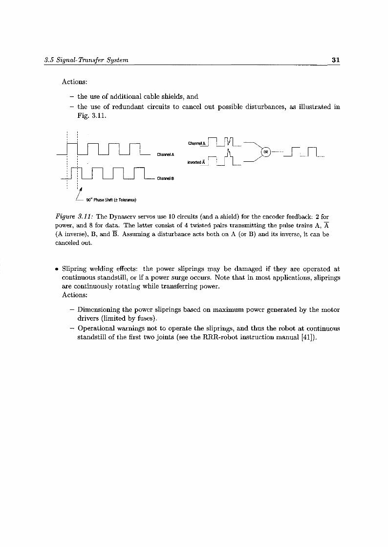
Actions :

- the use of additional cable shields, and- the use of redundant circuits to cancel out possible disturbances, as illustrated in

Fig. 3.11 .

Channel A

L- 90° Phase Shift (*Tolerance)

Channel A

I Channel B

Inverted Aj

Figure 3.11 : The Dynaserv servos use 10 circuits (and a shield) for the encoder feedback : 2 forpower, and 8 for data . The latter consist of 4 twisted pairs transmitting the pulse trains A, X(A inverse), B, and B. Assuming a disturbance acts both on A (or B) and its inverse, it can becanceled out .

• Slipring welding effects : the power sliprings may be damaged if they are operated atcontinuous standstill, or if a power surge occurs . Note that in most applications, slipringsare continuously rotating while transferring power .Actions :

- Dimensioning the power sliprings based on maximum power generated by the motordrivers (limited by fuses) .

- Operational warnings not to operate the sliprings, and thus the robot at continuousstandstill of the first two joints (see the RRR-robot instruction manual [41]) .

Chapter 4

Synthesis of subsystems

After the selection of appropriate components and design solutions in the previouschapter, now, all subsystems are combined . First, the design of the manipulatorframe is discussed . Next, the Control System is added, and an evaluation of thesystem is performed. Finally, the RRR-robot specifications are discussed.

4.1 Manipulator frame

Obviously, the design of the manipulator frame can not be separated from the previously dis-cussed subsystems. Especially, the Joint-Actuation System, the Measurement System, and theSignal-Transfer System are closely interconnected with the frame design. In Section 3 .2, aspecific series of servos was found which can satisfy the main requirement : maintaining highCoriolis and centrifugal torques . These so called "Dynaserv" motors are self-contained unitswith internal bearings and suitable joint angle-sensors (see Appendix B) .

Although restricting the designers freedom, the use of these complete servo-units can greatlysimplify and speed-up the design process . Therefore, a choice was made to design the manip-ulator frame starting with the three Dynaserv motors from Table 3 .1. The components of theslipring based Signal-Transfer System are selected in conjunction with the frame design basedon the available space and available commercial products .

In the following sections various design aspects are discussed . Leading to the conceptualdesign of Fig. 4.1 and Fig. 4.2 . Based on this design the CTD manufactured all non-standardcomponents (see Table 4 .2) .

4.1 .1 Motor load

The limiting factor in using the Dynaserv servos is the bending moment their bearings canhandle: 200 [Nm] for static load, and 60 [Nm] for alternating load . However, these limits arecalculated for a lifetime of 5 years, and continuous pick-and-place applications with a trapeziumshaped velocity profile. In the RRR-robot, the motors will be used for much shorter periods,but with larger accelerations. Therefore, it is preferable to design the robot for smaller loads .

34

4 . Rotor extension 0M34 .

10. H0us4na DM30

Synthesis of subsystems

Sionol sliprin0

71 . Stotar extensfon D

18 Sf noi s~l r

5 . Porer sl-(7 Porer

7 . 0 i5

9 . Bevin cover

8 . Bearinq 165-120

Rotor extens~an OM60

Si0na1BIiD~inO~

~

klm~ i I' . I . Base

~

22

Figure 4 .1 : RRR-Robot conceptual design, used as a basis for the realization of the various non-standard components . Note that some dimensions were slightly altered during the manufacturing

Table 4.1 : Moving parts : joints and links

part subcomponents mass [kg]Joint 1 DM60 12Link 1 (vertical) Rotor extension DM60, PSR-1, Housing 20 .6

DM30, and Stator extension DM30Joint 2 DM30 7.5Link 2 Rotor extension DM30, PSR-2 and Arm 2 8.9Joint 3 DM15 5.5Link 3 Arm 3 (not present) -

4.1 Manipulator frame 35

Figure 4.2: 3D view of the conceptual design .

Table 4 .2 : RRR-Robot main components (see Fig . 4.1) . With the exception of part 8, all partsmanufactured by the CTD are made of Aluminum. The masses are either measured, estimated,calculated (indicated with a *), or supplied by the manufacturer.

No. Part Source Mass [kg]1. Base CTD 15*2. Spherical joint CTD 2*3. Housing DM60 CTD 6*4. DM60 Litton (Appendix B.1) 125. Signal slipring 1 (SSR-1) Litton (Appendix B .3.2) < 0.16. Rotor extension DM60 CTD7. Power slipring 1 (PSR-1) Litton (Appendix B .3.1) 3.504

8. Bearing 165-120-22 CTD < 0 .59. Bearing cover CTD < 0.110. Housing DM30 CTD 15.511. Stator extension DM30 CTD 1.62012. DM30 Litton (Appendix B.1) 7.513. Signal slipring 2 (SSR-2) Litton (Appendix B .3.2) < 0.114. Rotor extension DM30 CTD 1 .48215. Power slipring 2(PSR-2) Litton (Appendix B.3.1) 3.46416. Arm 2 CTD 3.90817. DM15 Litton (Appendix B.1) 5.518. Signal slipring 3 (SSR-3) Litton (Appendix B .3.2) < 0.1

36 Synthesis of subsystems

The moment loads are caused by Coriolis and centrifugal forces acting perpendicular andparallel to the rotation axes. Motor 1 (4. DM60 in Fig . 4.1) is submitted to the largest forces,caused by its own rotation velocity, and acceleration ; and those of motor 2 and 3 (12. DM30and 17 DM17) . Since otherwise the specified load is exceeded, an additional (radial) bearing isneeded to reduce the moment load on motor 1 .

However, adding a second bearing causes Link 1(defined in Table 4 .1) to be kinematiclyoverdetermined, and thus imposes severe demands on its centering and alignment. The shaftmetal of the motor may get damaged if the centering offset remains 10 [µm] or more (see theDynaserv manual) . To bring down the kinematic degrees of freedom, a choice was made topartly "disable" the internal motor bearings . This can be achieved by mounting the motor ona membrane plate, or more practical on a spherical joint (2 . Spherical joint in Fig . 4.1) . Withthis solution, Motor 1 is completely discharged from moment load .

Motor 2 (12. DM30 in Fig. 4.1) is now subject to the largest Coriolis and centrifugal forces .In Fig. 4.3 the moment load on Motor 2 is plotted for two different loading directions . Theaccelerations are chosen to represent the largest values possible based on the inertia matricesand the maximum motor torque . As can be seen, the load remains well below 60 [Nm] if thechosen nominal motor velocities of 0 .5, 1 and 1 .5 [rps] are not exceeded .

Figure 4 .3: Moment load on motor 2 due to forces parallel and perpendicular to the rotationaxis. This load should remain below 60 [Nm] . Unless otherwise specified the velocities areq=[7r, 27r, 37r]T. Rotation angles and accelerations are set to represent worst-case values (themaximum accelerations are based on the inertia matrices) .

Bearing type For the additional radial bearing a large, and thus stiff ball bearing is selected(ball bearing CTD 165-120-22) based on the available space. The calculated worst-case life spanof this bearing is 1 .25 1012 revolutions . This is more than adequate considering the requiredtechnical lifespan of 5 years :

10 year x 40 weeks/year x 5 days/week x 1 hour/day x 3600 x 0 .5 rps = 3 .6 106 revolutions

4 .2 Measurement System : Cartesian measurement system 37

4.1 .2 Sliprings

Based on the specifications derived in Section 3 .5, and the chosen nominal motor velocities of0.5, 1 and 1 .5 [rps], sliprings are selected for data and power transfer .

Data

Although, sliprings suitable for both data and power transfer exist, the combination of high andlow power circuits complicates the selection . To satisfy the combined specifications, completelycustom made and thus expensive slipring units are required . Therefore, exploiting a specialfeature of the Dynaserv motors - the hollow core (Fig. B .1) - small signal sliprings are placedinside the motors .

In Table B.4, the main specifications of the selected sliprings are summarized. Signalslipring 3 (SSR-3) has n = 12 (> 8) circuits. For SSR-1, a sliprings with 36 circuits is se-lected (> 22 + 12) . Although less circuits are required, SSR-2 is chosen equal to SSR-1 becauseit is cheaper to order two identical sliprings than one with 36, and one with 24 circuits .

Note that the maximum sliprings velocities (1 .67, 1.67, and 2 [rps]) are below the maximumindividual motor velocities (2.4 [rps]) . Apart from the motor load, this is another reason tomaintain strict limitations on the motor velocities : 0.5, 1 and 1 .5 [rps] for motor 1, motor 2,and motor 3 respectively .

Power

With the use of an additional bearing (8 . Bearing 156-120-22), the total length of Link 1 is nolonger important. Therefore Power Slipring 1 (7 .) can be placed above Motor 1 . Based on thespecifications two off-the-shelve sliprings are selected (see Table B .3) .

However, the length of Link 2, and especially, the offset distance between Motor 2, and 3(parallel to their rotation axes) is relevant ; it determines the moment load on Motor 2 . Tominimize this distance, Power slipring 2 is placed around and behind motor 2 . In Table B .3, themain specifications of a modified, large diameter, slipring are summarized .

4.1 .3 Eigenfrequencies

The magnitudes of several eigenfrequencies were estimated using simple mass-spring models ofthe design . The lowest eigenfrequency, 79 [Hz], of the system emanates from the motor bearingsof the largest motor (the DM60) . All other eigenfrequencies - emanating from the sphericaljoint, Link 1, or Link 2 - are higher .

4.2 Measurement System : Cartesian measurement system

In Section 3 .3.3, the results of a survey of 3D tracking systems are summarized, and a recom-mendation is made to use a CCD-line camera based system . Since commercial systems are tooexpensive, this should be a custom-made, or even homebuilt system .

Designing, and building this system, however requires considerable time, and effort ; andtherefore has not yet been realized .


4.3 Evaluation

In this Section, the manipulator frame is combined with the Control System, and a model basedcontrol algorithm is implemented in Simulink to test the real-time performance of the controller .Next, several experimental results are discussed to evaluate the performance of the chosen servos .Finally, all RRR-robot specifications are discussed .

4 .3.1 Real-time performance

In Section 3 .4, a PC based controller was selected : the MultiQ I/O board in combination witha soft real-time operating system (Windows 3 .11). Although, this controller offers Matlab andSimulink integration, it may cause a variation in the effective sample frequency . In Fig. 4.4, theparameters determining the performance are defined .

n q ~ fT,FA w ~ 0

r

z ,.zzz zuO.a i i 0real-timeexecution (TT) :

- 3 x encoder in- calculate u

- 3 x DA out

foregroundtasks (Tf) :

- GUI

- other

Clockinterrupts

Latency

Actualperformance

T8 : desired sampling period (with the internal windows clock) .

Ti : latency, the time to stop the foreground tasks and start the real-time section .

Te : effective sampling time, with an average Tef and variance o(Te) .

T, . : time to execute the real-time code, e .g., generated from the blockdiagram shown in Fig . 4 .5 : read out the encoders, calculate thecontrol law, and send the calculated values to the DA converter .

Tf : time remaining for foreground tasks, e .g., the graphical user inter-face (GUI) of the controller .

Figure 4 .4: Parameters defining the real-time performance .

Using an internal or external timer, interrupts are generated with a desired sampling periodTs . When an interrupt occurs there is a latency Tl before the foreground tasks are stopped,and the real-time controller is executed, resulting in a varying effective sampling period Te . Thetime T,, to execute the real-time code should be less than the desired sampling period minus the

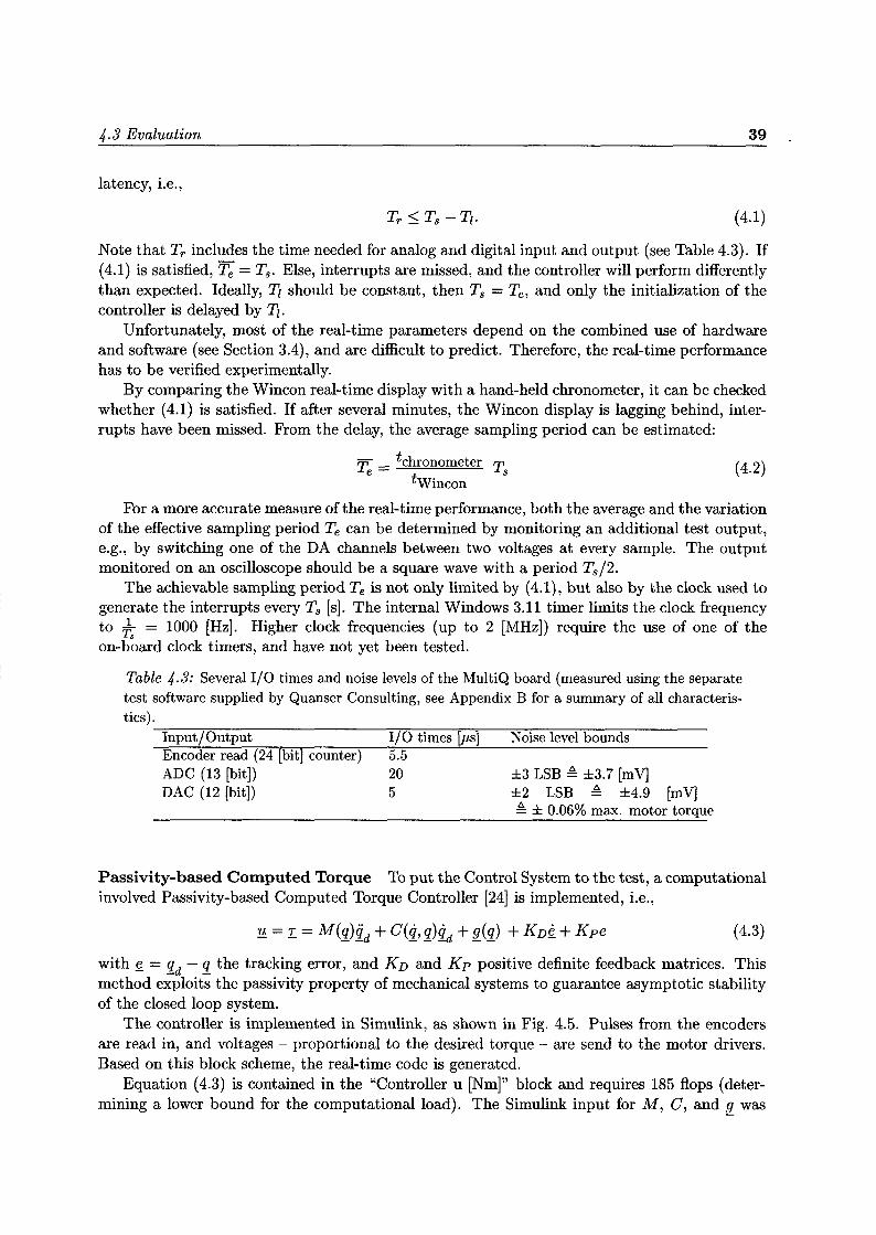
4.3 Evaluation 39

latency, i .e .,

T,. < Ts - Tl. (4.1)

Note that T,, includes the time needed for analog and digital input and output (see Table 4 .3) . If(4.1) is satisfied, Te = Ts . Else, interrupts are missed, and the controller will perform differentlythan expected . Ideally, Tl should be constant, then Ts = Te7 and only the initialization of thecontroller is delayed by Ti .

Unfortunately, most of the real-time parameters depend on the combined use of hardwareand software (see Section 3 .4), and are difficult to predict . Therefore, the real-time performancehas to be verified experimentally .

By comparing the Wincon real-time display with a hand-held chronometer, it can be checkedwhether (4 .1) is satisfied . If after several minutes, the Wincon display is lagging behind, inter-rupts have been missed . From the delay, the average sampling period can be estimated :

=tchronometer T (4.2)Te - t s

Wincon

For a more accurate measure of the real-time performance, both the average and the variationof the effective sampling period Te can be determined by monitoring an additional test output,e.g., by switching one of the DA channels between two voltages at every sample . The outputmonitored on an oscilloscope should be a square wave with a period Ts/2 .

The achievable sampling period Te is not only limited by (4 .1), but also by the clock used togenerate the interrupts every Ts [s] . The internal Windows 3.11 timer limits the clock frequencyto Ts = 1000 [Hz]. Higher clock frequencies (up to 2 [MHz]) require the use of one of theon-board clock timers, and have not yet been tested .

Table 4 .3 : Several I/O times and noise levels of the MultiQ board (measured using the separatetest software supplied by Quanser Consulting, see Appendix B for a summary of all characteris-tics) .

Input/Output I/O times [µs] Noise level boundsEncoder read (24 [bit] counter) 5 .5ADC (13 [bit]) 20 ±3 LSB °= ±3.7 [mV]DAC (12 [bit]) 5 ±2 LSB °= ±4.9 [mV]

°= ± 0.06% max. motor torque

Passivity-based Computed Torque To put the Control System to the test, a computationalinvolved Passivity-based Computed Torque Controller [24] is implemented, i .e.,

u= T= M(q)4, + C(q, q)qd + g(q) + KDg + Kpe (4.3)

with e = qd - q the tracking error, and KD and Kp positive definite feedback matrices. Thismethod exploits the passivity property of mechanical systems to guarantee asymptotic stabilityof the closed loop system .

The controller is implemented in Simulink, as shown in Fig . 4.5. Pulses from the encodersare read in, and voltages - proportional to the desired torque - are send to the motor drivers .Based on this block scheme, the real-time code is generated .

Equation (4.3) is contained in the "Controller u [Nm]" block and requires 185 flops (deter-mining a lower bound for the computational load) . The Simulink input for M, C, and g was


generated by Mathematica based on the rigid-robot model . This model has been refined usingthe inertia data generated by the CAD program Microstation (see Appendix A) .

nqdesl

1

qdes2 ^

qdes3trajectory

[qdes, qddes]

initializepos07 .m

RK3, 1000 HzKp = diag( [ 10 5 1]) ;Kd=diag([2050 .8]);

Pasivity Based Computed Torque Controller version : 07 Piotdate : 12-12-9

I

Kt MultiQ LlU [ MultiQ [q,qd] rad

in/out Nm-> 3 x DAC ~ ~ 3 x Encoder Differentiatelimit max(V) [ ~ and filter

RRR

x = [qi,q2,q3,qd1,qd2,qd3]

Figure 4.5 : The (top-level) Simulink block scheme of a Passivity Based Computed TorqueController .

Without AD conversions, the resulting I/O time is 31 .5 [ps] (see Table 4.3) . By monitoringa test signal (a block wave), it was verified that an effective sampling frequency of 1 [kHz] canbe achieved without missing interrupts, i .e ., Te = Ts . Furthermore, the variation of Te is smallerthan 0.05 [ms] . So, for the implementation of this computational involved (model based) controlalgorithm, the real-time performance seems adequate .

4.3.2 Servo performance

Torque vs command voltage Ideally, the relation between the command voltage and thetorque exerted by the motor is linear, i .e., Toutput = f (Ucommand) = Kt Ucommand . However,the exact value of Kt, or function f(Ucommand) is unclear. In Fig. 4.6, three motor outputrelations are shown for motor 2 : based on experiments and data supplied by two differentsuppliers of Dynaserv servos .

In the experiment, arm 2 is rotated at a very low (< 1[rpm]), but constant (controlled)velocity. The torque needed for this rotation can be determined from the combined gravity andfriction load, i .e., u2 = 14 .52 sin(q2) + T f2 [Nm], where T f2 is the (constant) coulomb frictiontorque. The resulting torque constant Kt = 6.7 . The friction torque Tf2 = u2(q2 = 0) ^ 3 [Nm] .The other two motor output relations are based on the (relative) saturation curve of Fig . B.2from Compuserve, and the torque constant stated by Litton (see Table B .1) .

The differences between these input-output relations are considerable, so in order to achievehigh performance tracking using model based control laws, more experiments (over the fulloutput range) are necessary to determine the correct functions f(Ucommand) for all three motors .

Furthermore, the friction torque of the Dynaserv servos (: 3 [Nm] for all three) is largerthan expected (Litton stated a friction torque of 5% of the maximum torque) . So for highperformance tracking, friction compensation is necessary as well .

4 .3 Evaluation 41

Motor 2: output torque vs . command voltage

Figure 4 .6: Output torque motor 2 as a function of the command voltage based on experiments,and data from two suppliers of Dynaserv servos (Litton [26] and Compumotor [9]) .

Model quality Figure 4 .7 shows a comparison for both experiments and simulation for thecomputed torque controller . The desired trajectory is qd =[7r t, 2 7r t-7r/2, 37r t]T with initialconditions q(0) = 0 [rad/s] are shown .

control inputs u(t)

, .6f, 0 .4~-0.2

0

0.8

~ 40Z 20~~ 0-20

"g 06 20I~~` I \ ../ ../N ._1 \ I Z~C', ,,.T ®yV V N 0

°'0.20 -20

4

0L-.__

2 3 4time [s]

2

2

3

3

4

3 4time [s]

47 7 7 4(0)

Figure .7: CTC controller, simulated and measured position errors and control inputs . Withtrajectory qd = [ r t, 2 r t- -/2, 37r t]T, and initial conditions q(0) = = 0[rad]


The simulations are performed with the enhanced rigid-robot model implemented in Math-ematica with an non compensated friction torque of 3 [Nm] for each motor .

The controller parameters were set for a slow response . Motor constant 2 is set to 6 .7 [Nm/V] .As can be seen, there are some appreciable differences between simulation and experiments,probably due to incorrect model parameter values .

Contribution Coriolis and centrifugal torques To obtain an indication of the perfor-mance, ratio r (2 .2) is evaluated by substituting measured positions, velocities and accelerationsinto the model. Two links have a ratio of 0 .5 or more : r=[0.76, 0 .32, 0 .83] .

The presence of friction obviously reduces the contribution of the Coriolis and centrifugaltorques. But even if the friction torque is included into ratio r, the performance ratio of link 1remains above 0 .5 .

4.3 .3 Design specifications

In this Section the RRR-robot specifications (Section 2 .3), and thus the main features of thecombined subsystems, are discussed . Although the robot is designed to satisfy all requirementsof Section 2 .3, currently, the requirements with regard to the static, and dynamic end-effectoraccuracy (requirements (4) and (5)) are difficult to evaluate because of the absence of a Cartesianmeasurement system for the end-effector .

Design requirements

(1) By using sliprings to facilitate unconstrained rotation, and direct-drive servos, the Cori-olis and centrifugal torques on at least one link can be made sufficiently large (see theexperimental results of Section 4 .3.2) .

(2) The actuator torques are a direct function of the command signals . However, this functionis possibly non-linear (see Fig . 4.6), and remains to be measured .

(3) The RRR-robot has three rotational degrees of freedom .

(4) The accuracy of joint-angle sensors (±15 [arc-sec]) should - after kinematic calibration -enable a static end-effector accuracy of e= [Ox, Ay' AZ]T = [0.036, 0.036, 0.058]T [mm] .

(5) Assuming all joint and links are rigid (no unintentional flexibilities), a lower bound for theabsolute end-effector le(t)1, could be determined by observing the tracking behavior of awell tuned controller . However, this kind of fine tuning has not yet been performed .

(6) The third link is exchangeable with a flexible one .

(7) A torsionally flexible element (see, e .g., [32]) can be attached to the third servo (or joint),thus transforming it into a flexible drive .

(8) The control interface is based on Simulink (and Matlab) .

(9) The characteristic dimension - the length of Link 1 - is 0.5 [m] ;

(10) The technical lifespan of all components is at least 10 year .

(11) If the Cartesian measurement system is be realized with NLG 50K, the (expected) total re-alization cost is about fl 160 .000,-, slightly exceeding the original budget (see Appendix C) .

(12) Because of its size, the robot is suitable for demonstrations for a group of at least 10people .

4.3 Evaluation 43

(13) The system is made safe for operators and spectators by means of electrical shielding andrestricting the access to the robot's workspace .

4 .3.4 Design goals

With respect to the design goals, the RRR-robot has the following features :

(a) Modern, state-of-the-art techniques and components are used : compact direct-drive servos,miniaturized signal sliprings, and automated real-time code generation .

(b) On Link 3, 12 channels are available for additional sensors .

(c) The RRR-robot has the same structure as the familiar "Puma"-type industrial manipulator(without a wrist) .

(d) Maintenance is restricted to cleaning the contacts of the power sliprings . Both units canbe reached by simply removing the brushblocks .

(e) For demonstration purposes, each link has a separate color. In addition, the power slipringbrushblock terminals have Plexiglas covers .

Chapter 5

Conclusions and recommendations

5.1 Conclusions

Result An industrial-like experimental facility, the RRR-robot, has been realized that offersthe ability to enhance Coriolis and centrifugal torques relative to other nonlinear effects . Twoimportant features of the RRR-robot were introduced in order to reach this design goal : uncon-strained rotation of each link by using sliprings, and the use of direct-drive servos. Although,the friction torques of these servos are larger than expected, the contribution of the Coriolis andcentrifugal torques on one link can be made sufficiently large . A rigid-robot model has beenimplemented in Mathematica to aid servo sizing. Using the CAD package Microstation, thismodel has been refined for simulation purposes, and to aid in the implementation of controllersby generating Simulink input .

Mrame design The robot has a modular setup, i .e., it has been designed starting from aspecific type of servo with internal bearing, and angular sensors . The last link can be replacedby a flexible link, and the last joint can be transformed into a flexible joint . Thus making itsuitable to evaluate control schemes for both rigid-robots and flexible joint and/or link robots .

Control System The RRR-robot is equipped with a Simulink based graphical user interface,offering optimal flexibility to the user . The computational power of this Control System hasbeen demonstrated by implementing a model based control algorithm . Several provisions havebeen made to provide safety for operators and spectators, but also to prevent damage due tooperator mistakes or controllers that destabilize the closed loop system .

Cartesian measurement system Considering the combination of high accuracy, high up-date rate and uninterrupted tracking only one separate technology is suitable for tracking theend-effector of the RRR-robot : vision based ranging using multiple line-array cameras . Sinceavailable commercial system exceed the available budget (NLG 50K) by a factor 4, this shouldbe a custom-made or even homebuilt system . Designing and building this system requires con-siderable effort . Although, several (engineering) firms were contacted, a Cartesian measurementsystem has not yet been realized . As a consequence, the required static and dynamic positionaccuracy has not yet been validated .

- 45 -

46 Conclusions and recommendations

Budget Comparing the expenses, and the original budget (Appendix C), the Control System(posts 4 and 5), and the Joint-Actuation System together with the Signal-Transfer System (post2) both turned out to be cheaper . The construction of the frame parts, especially the shieldingof the motor drivers (required by law) resulted in considerable larger expenses than anticipated .If the budget for the Cartesian measurement system remains unchanged, the total budget willbe exceeded by approximately 5% .

5.2 Recommendations

In its present state, the RRR-robot can be used to evaluate rigid-robot controllers in the jointspace. To evaluate control algorithms for flexible joint and/or link robots, and to calibrate therobot, additional components are required :

• an optical measurement system (using line-array cameras) to determine the Cartesianposition of the end-effector,

• a flexible third link, and

• a flexible third joint .

Furthermore, a number of parameters must be determined experimentally :

• the exact (Denavit-Hartenberg) construction parameters (kinematic calibration),

• the motor input-output characteristics (Kt) and motor dynamics (e .g., torque ripple),

• the motor (and joint) friction (T f), and

• the rigid-robot model parameters in M, C, and g .

Future research may involve the systematic evaluation of several control algorithms for rigid,and flexible joint and/or link robots . Besides encoder feedback, non-colocated actuation/sensing(using additional link sensors) and vision feedback schemes can be implemented .

Appendix A

Modeling the RRR-robot

A.1 Introduction

A model of the RRR-robot is needed for a number of different reasons : as a design tool (e .g .,choosing the right servos), as a simulation model for control design, and for control synthesisand implementation . Each application imposes different requirements, and for all specializedsoftware packages exist .

In this appendix, however, a general purpose and conceptually straightforward modelingapproach is described . This approach can be easily implemented in a symbolic manipulationpackage, and results in an explicit model . Although the computational efficiency of this generalpurpose model is low, it can be used for all applications mentioned above .

First a rigid body model is derived using the Denavit-Hartenberg convention to describe thekinematics in a systematic manner . Assuming small deflections of the links, this conventioncan be extended to a generalized flexible link model (section A .3) . Finally, in section A .4 someimplementation issues are discussed .

A.2 Rigid manipulator model

The first step in modeling a manipulator is formulating the kinematics, the relation betweenthe joint-angle space and the position and orientation of each arm with respect to a inertialreference frame .

Depending on the formulation of the kinematic relationships, a distinction is made betweenthe direct kinematics problem and the inverse kinematics problem . To derive the dynamic modelthe direct kinematic problem is solved, i.e., the position and orientation of the end-effector isexpressed as a function of the joint coordinates . The inverse problem is important to transformthe desired motion of the end-effector in the workspace into the required joint motion . However,it is not dealt with here .

Based on the (direct) kinematic model, various formulations (such as Euler-Lagrange ord'Alembert) can be used to derive the dynamics.

A.2 .1 Direct kinematics

A computational convenient method to describe the kinematic relationships is a vector-matrixdescription. The direct kinematic problem is then to find a transformation matrix that relatesa body-attached coordinate frame to the reference coordinate frame .

- 47 -

48 Modeling the RRR-robot

To include both rotations and translations (and, if desired, scaling), a 4 x 4 homogeneoustransformation matrix can be used [25] . This transformation matrix, A, maps an augmentedposition vector p expressed in homogeneous coordinates (p =[px, py, pz,1]) from one coordinatesystem to another. For robotic applications this homogeneous transformation matrix is givenby :

A_ 3 x 3 rotation matrix 3 x 1 translation vector (A.1)

0 0 0 1

A minimum of four parameters is needed to describe this transformation: two distances, a andd, and two angles, a and q. If coordinate frames are attached to each rigid link of a manipulator,the position and orientation of frame Oi with respect to a previous frame Oi-1 is given by :

Ai'-1(qZ) =

cos(qi) - cos(ai) sin(qi) sin(ai) sin(qi) a2 cos(q2)sin(q2) cos(ai) cos(qz) - sin(ai) cos(qi) ai sin(qi)0 sin(ai) cos(ai) di0 0 0 1

(A .2)

For a kinematic chain, the coordinate transformation To (a, d, a, q) from any link frame On tothe base coordinate frame 00 is given by the product of homogeneous transformation matrices,i.e .,

Tó (q) = AoAi . . . Ann-1 (A.3)

As a result the kinematic configuration of a rotational manipulator is completely described bythree constant parameter vectors (a, d and a) depending on the geometry of the robot, anda vector with the joint rotations q. Using this transformation all link properties (such as thecenter of gravity and the link or motor inertia) defined in their own link coordinates, can beexpressed in base coordinates . Thus in terms of the fixed inertial coordinate of the base, theposition of a point on link i is given by :

hp = Tp hi (A.4)

Denavit and Hartenberg proposed a convention to choose the link coordinate frame system-aticly. For the RRR-robot this is shown in Fig . A .1 . In Table A .1 are the DH-parameters for anideal robot with perfect parallel or perpendicular axes .

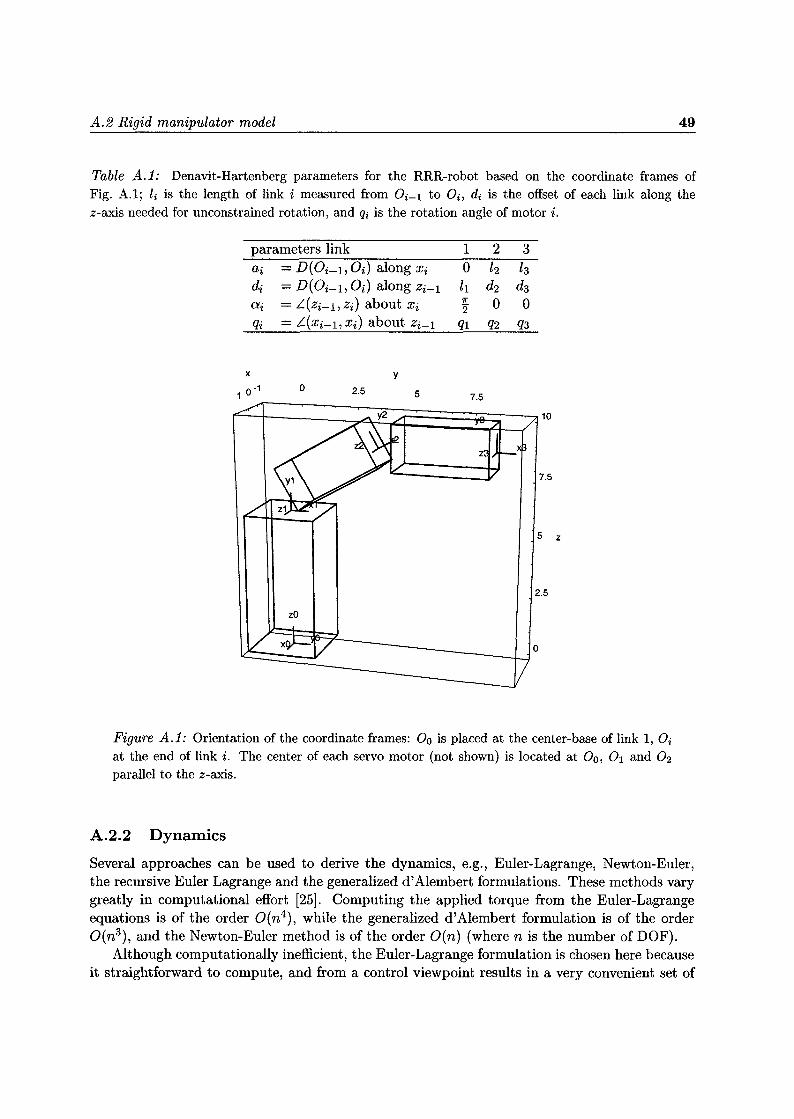
A. 2 Rigid manipulator model 49

Table A .1 : Denavit-Hartenberg parameters for the RRR-robot based on the coordinate frames ofFig. A.1 ; li is the length of link i measured from 0i_1 to Oi, di is the offset of each link along thez-axis needed for unconstrained rotation, and qj is the rotation angle of motor i .

parameters link 1 2 3ai = D(OZ_l, OZ) along xi 0 12 13di = D(OZ-1, OZ) along z2-1 li d2 d3ai = L(z2_1, z2) about xi 2 0 0qi = L(x2_l, xi) about zi-i qi q2 q3

0 2 .5

Y

5 7 .5

Figure A .1 : Orientation of the coordinate frames : Oo is placed at the center-base of link 1, Oiat the end of link i . The center of each servo motor (not shown) is located at 00, 01 and 02parallel to the z-axis .

A.2 .2 Dynamics

Several approaches can be used to derive the dynamics, e .g., Euler-Lagrange, Newton-Euler,the recursive Euler Lagrange and the generalized d'Alembert formulations . These methods varygreatly in computational effort [25] . Computing the applied torque from the Euler-Lagrangeequations is of the order O(n4), while the generalized d'Alembert formulation is of the orderO(n3), and the Newton-Euler method is of the order 0(n) (where n is the number of DOF) .

Although computationally inefficient, the Euler-Lagrange formulation is chosen here becauseit straightforward to compute, and from a control viewpoint results in a very convenient set of


(closed-form) equations :

M(q) q+ C(q, q) 4+ g(q) =,r (A.5)

where, M is the inertia matrix, C( q, q) q accounts for the Coriolis and centrifugal torques, g arethe conservative torques due to gravity, and ?- accounts for all non-conservative torques (suchas control input or friction) .

The dynamic coefficients M, C, and g can be determined from the Lagrangian L = Uk - UP(see [24, 25]),

d 8L-

OLdt C 8qi qi = Ti'

i = 1 . . . n links (A.6)

In the following paragraphs the expressions for the kinetic energy, U k , and the potential energy,Up, are addressed briefly. Finally the resulting dynamic coefficients are stated .

Kinetic Energy The kinetic energy of a point on the i-th link is

dUk, = 2 dm Tr(ho hoT ) (A.7)

where dm is the differential mass, and Tr( .) the trace operator . Substituting (A .4), integratingeach link over its entire mass and summing over all, n, links results in the total kinetic energy,Uk with respect to the inertial frame :

f i

Uk

_~• J dUk~ _~. J l ~~~ J a7o Ji (aIi)o Tqj qk

}} (A.8)iL=1• il-Jl 1 2 j=i kL=•1 l aq

j aq k

where Ji is the total inertia matrix of link i with respect to the base frame.

Potential Energy Expressed in the base coordinate frame the potential energy is given byn n

ri (A.9)up =~ upi G n'i=i i=1

where Li is the center of mass of link i in the link coordinate frame and G is the gravity vector .

Dynamic coefficients

Ciik =

Mik =

n n ~~ a2Tó J C~To 1 T 1~ L. Ciqkaqm ~ aq J Jim=1 j=max(i,k,m)

n j

gi =E -mj G9q j(C áT0 1

rj (A.12)i

j=max(i,k)

j=i

OTj

qk

j3 C ~0/T~~a(A.10)

(A.11)

for i, k, m= 1 . . . n links .

A .3 Flexible model 51

A.2 .3 Inertia parameters

After completion of the robot, Microstation Modeler was used to generate a 3D model of therobot in order to calculate the inertia tensors of each joint-link pair expressed in the appropriatelink coordinates. In Table A .2, all moving components are grouped to form joints (the motors)and links with appropriate link coordinate frames.

Table A. 2: Moving parts (joints and links) and the placement of the coordinate frames .partJoint 1Link 1 (vertical)

Joint 2Link 2 (green)Joint 3Link 3

subcomponents mass [kg]DM60 12Rotor extension DM60, PSR-1, Housing 20 .6DM30, and Stator extension DM30DM30 7.5Rotor extension DM30, PSR-2 and Arm 2 8 .9DM15 5.5Arm 3 (not present) -

Placement of the coordinate frames (see Fig. A.1 for the orientations) :

. Oo at the center-base of link 1 .• 01 at he intersection of the DM60 and DM30 rotation axes .

• 02 at the intersection of the DM15 rotation axis and the line parallel to the length axis ofArm 2, through its center of gravity.

. 03 at the end of the line parallel to the length axis of Arm 3 through its center of gravity .Note that Arm 3 is not yet present, so 03 is located at the end of a virtual link with length0.3 [m] .

The combined inertia tensor of Link i and Joint i with respect to frame i is given by Jz :

J1 =

J2 =

2.2334 -2.656010-7-2.656010-7 0 .22132.775510-$ -0.014560 -6.1425

2 .775510-$ 0-0.01456 -6.14252.2623 -0.2270-0.2270 32.9305

0.1921 1.9029 10-4 -0.2068 -2.84391 .902910-4 0.7340 0 0-0.2068 0 0.6474 -1 .0222-2.8439 0 -1.0222 16.3123

0.01238 0 0 0_ 0 001190 0 0

J3 0 0* 0.012 00 0 0 5.4763

A.3 Flexible model

(A.13)

(A.14)

(A.15)

Many studies of flexible manipulators have concentrated on the single-joint, single link example,e.g., [22, 38] . Link flexibility is modeled by a Bernoulli-Euler beam with a truncated number ofmodal coordinates .

Although, some researchers [5] stress the importance to move into more realistic 2 and 3joint experiments where flexibility is representative of real applications or at least scaled to


those applications, much less literature deals with modeling and control of these multi-linkmanipulators. Mainly because of the highly complicated algebraic manipulations involved .

Dynamic modeling of multi-link manipulators can be divided into two groups :

1. finite element based methods, and

2. assumed modes based models .

Finite element based methods [28, 18] can be applied to complex shaped systems . However theydo not give much insight to the dynamic structure of the system .

Book [4, 6] and Cetinkunt [7, 8] developed a general Lagrangian-assumed modes basedmethod. It uses 4 x 4 homogeneous transformation matrices to include both joint and deflectionmotion. The resulting dynamic model has a form similar to the previous discussed rigid manip-ulator model . In the following subsection the basic idea behind flexible kinematics is discussed .The implementation of flexible-arm dynamics is analogue to the rigid case .

A.3 .1 Flexible-arm kinematics

The transformation from a point on a flexible arm to the base coordinates can be separated intotwo steps: a transformation, A, due to the joint rotation, and a transformation, E, due to the(small) link deflection :

hp = To' hi = A0' E" AiEi . . . An_1r%n-1 hi (A.16)

The joint transformation matrix Ai-1(q) is identical to (A.2) .To incorporate the deflection of the link, the approach of modal analysis is used . This

approach is valid for small deflection of the link . A coordinate system Oez = [xi, yi, zi] is chosenat the base of the link with the x-axis coincident with the neutral axis . With 'q as a coordinatealong this neutral axis a point on the link is given by

77001

(A.17)

where Jij is the time varying amplitude of mode j of link i; xij, yij, and zij are the displacementcomponents; and mi is the number of modes of link i .

If the deflections are small so are the rotation components [Bxij, Byij, Bzij], and the transfor-mation E(B) is given by

Ez_1(8) _

1 0 0 li ~0 1 0 00 0 1 00 0 0 0

A.4 Implementation

F 0

eyij

0

-Bz2j oyij „,ij -0 exij Yij (A.Bxij 0 zij

0 0 0-

18)

To derive a simulation model of the robot several multi-body packages exist . Some commercialproducts like Adams can be integrated with CAD packages and even with Matlab/Simulink .

A .4 Implementation 53

However, none of them is directly suitable for control purposes [39] . The output consists of aimplicit model including differential algebraic equations .

For optimal flexibility Mathematica [45] was used to generate the resulting equations of mo-tion. Implementing for example (A. 10) in this symbolic manipulation package is straightforward :

Mik[i_,k_] := Sum[ Tr[D[T[j],q[[k]]] .J[j] . Transpose[ D[T[j],q[[i]]] ]],{j,Max[i,k],n} I

Appendix B

RRR-robot components

In this Appendix, The main features of the used components are listed . For moredetailed information (e .g., contact information) refer to the RRR-robot instructionmanual [41] .

B.1 Dynaserv servos

The Dynaserv [26] motors are self-contained units containing precision ball bearings, magneticcomponents, and integral feedback . The rotor is placed around the stator (outer-rotor), pro-viding direct motion to the outside of the motor . On the inside, the motor has a hollow core(diameter 25 [mm]) which is part of the rotor . With regard to the stator, only the base part isvisible .

LED VitClamp Ring

Mausïng Kit r,_IRetaining IRing IStator G _are

Figure B. 1 : On the left, Dynaserv motor v .s. a conventional motor ; and on the right, an explodedview of the Dynaserv servo .

trtreet Drive~ E~M«

In Table B.1, the main specifications of the motors are summarized . The listed maximumtorque and maximum velocity cannot be achieved simultaneously, as illustrated in Fig . B .2 .

56 RRR-robot components

Table B . 1 : Main specifications of the Dynaserv motors . Source: Dynaserv manual and personalcommunications with Litton (marked by *) .

property unit

max. output torque [Nm]max. velocity [rps]mass [kg]inertia [kg m2]allowed axial load [N]allowed moment load [Nm]allowed velocity [rps]torque constant* [Nm/V]max. power [kW]

" DM Series B Type Motors (240V)56

49

42

35

LF 28°921

14

7

0,5 t p t.aS~ ~)

zo

DM60 DM30 DM15Motor 1 Motor 2 Motor 360 30 152.4 2.4 2.412 7.5 5.50.023 0.015 0.0123 10 (compression), 3 10 (tension)200 (static load), 60 (alternating load*)0.5 1 1.515.6 7.8 3.92.2 2.0 1.6

2,S

Figure B.2 : On the left, the DM series motor performance (torque v .s. velocity), on the rightthe saturation of the motor output torque as as a function of the command voltage send to thedriver (source: Compumotor [9]) .

B.2 MultiQ plug-in and terminal board

The MultiQ I/O board from Quanser Consulting [10] and its terminal board are shown inFig. B.3. Its main characteristics are summarized in Table B .2 .

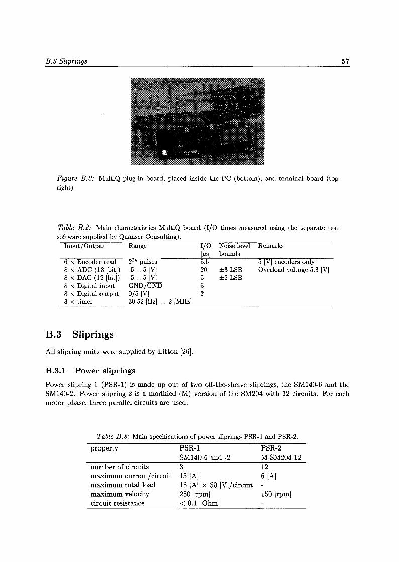
B.3 Sliprings 57

Figure B.3: MultiQ plug-in board, placed inside the PC (bottom), and terminal board (topright)

Table B.2: Main characteristics MultiQ board (I/O times measured using the separate testsoftware supplied by Quanser Consulting) .

Input/Output Range I/O Noise level Remarks[µs] bounds

6 x Encoder read 2 24 pulses 5.5 5 V encoders only8 x ADC (13 [bit]) -5 . . . 5 [V] 20 ±3 LSB Overload voltage 5 .3 [V]8 x DAC (12 [bit]) -5 . . .5 [V] 5 ±2 LSB8 x Digital input GND/GND 58 x Digital output 0/5 [V] 23 x timer 30 .52 [Hz] . . . 2 [MHz]

B.3 Sliprings

All slipring units were supplied by Litton [26] .

B.3 .1 Power sliprings

Power slipring 1 (PSR-1) is made up out of two off-the-shelve sliprings, the SM140-6 and theSM140-2. Power slipring 2 is a modified (M) version of the SM204 with 12 circuits . For eachmotor phase, three parallel circuits are used .

Table B.3 : Main specifications of power sliprings PSR-1 and PSR-2 .

property PSR-1 PSR-2SM140-6 and -2 M-SM204-12

number of circuits 8 12maximum current/circuit 15 [A] 6 [A]maximum total load 15 [A] x 50 [V]/circuit -maximum velocity 250 [rpm] 150 [rpm]circuit resistance < 0.1 [Ohm] -

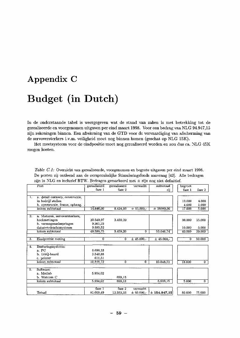
Appendix C

Budget (in Dutch)

In de onderstaande tabel is weergegeven wat de stand van zaken is met betrekking tot degerealiseerde en voorgenomen uitgaven per eind maart 1998 . Voor een bedrag van NLG 94.947,15zijn rekeningen binnen. Een afrekening van de GTD voor de vervaardiging van afscherming vande servoversterkers i.v.m. veiligheid moet nog binnen komen (geschat op NLG 15K) .

Het meetsysteem voor de eindpositie moet nog gerealiseerd worden en zou dus ca. NLG 45Kmogen kosten .

Table C. 1 : Overzicht van gerealiseerde, voorgenomen en begrote uitgaven per eind maart 1998 .De posten zij ontleend aan de oorspronkelijke Stimuleringsfonds aanvraag [42]. Alle bedragenzijn in NLG en inclusief BTW . Bedragen gemarkeerd met ± zijn nog niet definitief .Post gerealiseerd

fase 1gerealiseerd

fase 2verwacht subtotaal

rij

1 . a . detail ontwerp, constructie,in bedrijf stellenb. constructie, frame, ophang .kolom subtotaal 14.646,00 8.434,00 ± 15 .000,- f 38080,00

2 . a. Motoren, servoversterkers,hoekmetingenb. vermogenssleepringendataoverdrachtssysteem

30.540,979.361,239 .685,52

3.459,20

kolom subtotaal 49.586,75 3.459,20 0 53.046,74

3 . Eindpositie meting 0 0 ± 45.000,- t 45.000,-

4 . Besturingssysteem :a. PCb. DAQ-boardc. printer

6 .696,333 .540,88611,51

kolom subtotaal 10 .848,72 0 0 10.848,72

5 . Software :a. Matlabb. Watcom C

5.934,02699,13

kolom subtotaal 5.934,02 699,13 6.633,15

Totaalfase 1

81.009,49fase 2

12.593,33verwacht

± 60.000,- f 154.947,15

begrootfase 1 fase 2

13.000 4.0004.000 1.000

17.000 5.000

30.000 15.000

10.000 5.00040.000 20.000

( 0 50.000

18.000

5.000

0

0

80.000 75.000I

- 59 -

58

B.3 .2 Signal sliprings

~

RRR-robot components

Figure B.4: Signal sliprings : on the left, a photograph of the original AC-267 slipring ; in themiddle, the AC-267 inside a hollow mounting cylinder for gluing it inside the motors (used forSSR-1 and SSR-2) ; and on the right, SSR-3.

Table B.4 : Main specifications of the signal sliprings (see Fig . B.4) .

property SSR-1 and 2Capsule AC-267 modified

number of circuits 36maximum current/circuit 1.2 [A]maximum total load 25 [A]maximum velocity 100 [rpm]total friction torque 0 .0054 [Nm]

SSR-3Litton 12-ring capsule121 [A]50 [W]120 [rpm]0 .0023 [Nm]

Appendix D

Time schedule

Main activities and decision moments :

January 1996

• Start of the RRR-robot design project .

April 1996

• Implementation of a simple rigid-robot model in Mathematica .

• Evaluation of the original specifications .

July 1996

. Decision to order a PC-based control system : PC, DAQ board and software .

October 1996

• Selection of direct-drive servos using a refined rigid-robot model .

• Start concept design of the manipulator frame .

November 1996

• Decision to use sliprings for both power and data transfer .

December 1996

• Decision to order 3 servos .

• Decision to order 5 sliprings units for power and data transfer .

February 1997

• Order of slipring units for data transfer was "lost", and had to be reiterated .

• Decision to skip the detail design by the CTD and start of manufacturing of frame partsbased on the concept design .

- 61 -

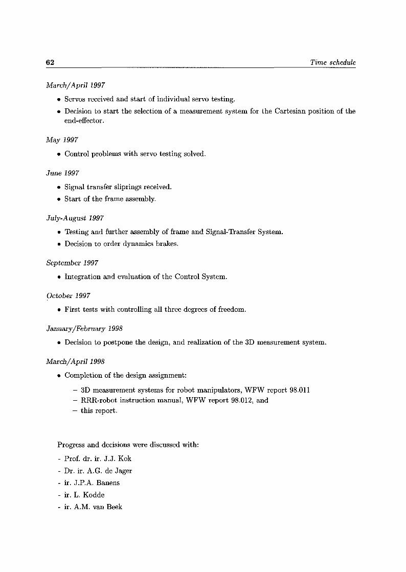
62 Time schedule

March/April 1997

• Servos received and start of individual servo testing .

• Decision to start the selection of a measurement system for the Cartesian position of theend-effector .

May 1997

• Control problems with servo testing solved .

June 1997

• Signal transfer sliprings received .

• Start of the frame assembly.

July-August 1997

• Testing and further assembly of frame and Signal-Transfer System .

• Decision to order dynamics brakes .

September 1997

• Integration and evaluation of the Control System .

October 1997

. First tests with controlling all three degrees of freedom .

January/February 1998

. Decision to postpone the design, and realization of the 3D measurement system .

March/April 1998

• Completion of the design assignment :

- 3D measurement systems for robot manipulators, WFW report 98 .011- RRR-robot instruction manual, WFW report 98.012, and- this report .

Progress and decisions were discussed with :

- Prof. dr . ir. J.J . Kok

- Dr. ir. A.G . de Jager

- ir . J .P.A. Banens

- ir. L . Kodde

- ir. A.M. van Beek

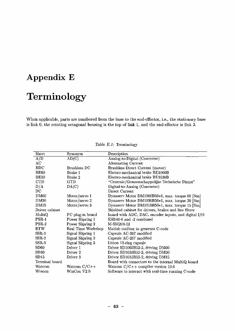
Appendix E

Terminology

When applicable, parts are numbered from the base to the end-effector, i .e., the stationary baseis link 0, the rotating octagonal housing is the top of link 1, and the end-effector is link 3 .

Table E.1 : Terminology

Short Synonym DescriptionA/DACBDCBE60BE30CTDD/ADCDM60DM30DM15Driver cabinetMultiQPSR-1PSR-2RTWSSR-1SSR-2SSR-3SD60SD30SD15Terminal boardWatcomWincon

AD(C)

Brushless DCBrake 1Brake 2GTDDA(C)

Motor/servo 1Motor/servo 2Motor/servo 3

PC plug-in boardPower Slipring 1Power Slipring 2Real Time WorkshopSignal Slipring 1Signal Slipring 2Signal Slipring 3Driver 1Driver 2Driver 3

Watcom C/C++WinCon V2 .0

Analog-to-Digital (Converter)Alternating CurrentBrushless Direct Current (motor)Electro-mechanical brake BE1060BElectro-mechanical brake BE1030B"Centrale/Gemeenschappelijke Technische Dienst"Digital-to-Analog (Converter)Direct CurrentDynaserv Motor DM1060B50*1, max. torque 60 [Nm]Dynaserv Motor DM1030B50*1, max. torque 30 [Nm]Dynaserv Motor DM1015B50*1, max . torque 15 [Nm]Shielded cabinet for drivers, brakes and line filtersboard with ADC, DAC, encoder inputs, and digital I/OSM140-6 and -2 combinedM-SM204-12Matlab toolbox to generate C-codeCapsule AC-267 modifiedCapsule AC-267 modifiedLitton 12-ring capsuleDriver SD1060B52-2, driving DM60Driver SD1030B52-2, driving DM30Driver SD1015B52-2, driving DM15Board with connectors to the internal MultiQ boardWatcom C/C++ compiler version 10 .6Software to interact with real-time running C-code

Bibliography

[1] Gerry B. Andeen . Robot design handbook . McGraw-Hill, London, 1988 .

[2] Haruhiko Asada and Kamal Youcef-Toumi . Direct-drive robots . MIT press, London, 1987 .

[3] Open DeviceNet Vendor Association. DeviceNet . http://www.odva.org, 1998 .

[4] W. J. Book. Recursive Lagrangian dynamics of flexible manipulators . InternationalJournal of Robotics Research, vol. 3(no . 3) :87-101, 1984 .

[5] W. J. Book. Modeling, design, and control of flexible manipulator arms : A tutorialreview. In Proceedings of the 29th Conference on Decision and Control, volume 3, pages500-506. IEEE, 1990 .

[6] W. J. Book. Controlled motion in an elastic world . Dynamic Systems, Measurements, andControl, vol. 115:252-261, 1993 .

[7] S. Cetinkunt and W. J. Book. Symbolic modeling of flexible manipulators. In Proceedingsof 1987 IEEE International Conference on Robotics and Automation, volume 3, pages2074-2080, 1987 .

[8] S. Cetinkunt and W. J. Book. Symbolic modeling and dynamic simulation of roboticmanipulators with compliant links and joints . Robotics & Computer-IntegratedManufacturing, vol. 5(no. 4) :301-310, 1989 .

[9] Compumotor. Electronic motion control . http://www.compumotor.com, 1998 .

[10] Quanser consulting . Wincon and MultiQ . http://www.quanser.com, 1998 .

[11] N. Costescu and D. Dawson. QMotor 2 .0 - A PC based real-time multitasking graphicalcontrol environment . Submitted to IEEE Control Systems, 1997. Available athttp: //ece.clemson.edu/crb/research/qmotor/qmotor2.pdf.

[12] B. de Jager . Practical evaluation of robust control for a class of nonlinear mechanicaldynamic systems . PhD thesis, Eindhoven University of Technology, 1992 .

[13] E. O. Doebelin . Measurement systems: Application and design . McGraw-Hill, London,1990 .

[14] dSpace . DS1102 DSP controller board . http://www.dspace.de, 1997 .

[15] J . R. Gyorki. Making connections with factory-floor networks . Machine Design, 6:56-61,1996 .

- 65 -

66 BIBLIOGRAPHY

[16] Herbert Hanselmann . Guest editorial : Introduction to the special issue on digital signalproessors in control . In IEEE Transactions on Control Systems Technology, volume 5,pages 277-278, 1994 .

[17] Inc HD Systems . Harmonic drives (actuators). http://www.hdsystemsinc.com, 1998 .

[18] S. K. Ider and F . M. L . Amirouche. Nonlinear modeling of flexible multibody systemsdynamics subjected to variable constraints . Journal of Applied Mathematics, vol. 56 :444-450, 1989 .

[19] The MathWorks Inc. Matlab, simulink and the real-time workshop .http://www .mathworks.com, 1998 .

[20] Texas Instruments . TMS320C4X user's guide, 1993 .

[21] Gerald Jacob. Revisiting data acquisition configurations . EE-Evaluation Engineering,pages 22-28, 1987 .

[22] T . R. Kane, R. R. Ryan, and A . K. BanerJee. Dynamics of a canterlever beam attachedto a moving base . Journal of Guidance, vol. 10(no. 2) :139-151, 1987 .

[23] I. M. M. Lammerts, F . E. Veldpaus, J. J . Kok, and M . J. G . Van de Molegraft. Adaptivecomputed torque computed reference control of flexible robots . In ASME 1993 Winterannual meeting, New Orleans, Louisiana, USA, December 1993 .

[24] Ivonne M . M. Lammerts . Adaptive computed reference computed torque control of flexiblemanipulators . PhD thesis, Eindhoven University of Technology, 1993.

[25] C . S. G. Lee. Robots kinematics, dynamics and control. IEEE Computer, vol. 15(no. 12) :62-80, 1982 .

[26] Litton. Dynaserv sevos, µFORS-36 gyroscope, and various sliprings .http://www.litton.com, 1997. No online datasheet .

[27] QNX Software Systems Ltd . QNX realtime OS. http://www.qnx.com, 1997.

[28} F . Melzer. Symbolic computations in flexible multibody systems . Nonlinear Dynamics,(no. 9) :147-163, 1996 .

[29] NSK. Megatorque stepper motors . http://www.nsk.com, 1998. No online datasheet .

[30] Profibus. Process field bus . http://www.profibus .com, 1998 .

[31] T. M. Rosenberg. Industrial networks : The options and rewards are many. I&CS, 3 :61-66, March 1996 .

[32] P.C .J.N. Rosielle and E.A.G. Reker . Constructieprincipes 1 : bedoeld voor het nauwkeurigbewegen en positioneren . Technische Universiteit Eindhoven, Vakgroep PrecisionEngineering, Dictaat 4007, 1997 .

[33] Schleifring . Contactless optical and electrical transmission systems .http://www.schleifring .de, 1998 .

BIBLIOGRAPHY 67

[34] Lorenzo Sciavicco and Bruno Siciliano . Modeling and control of robot manipulators .McGraw-Hill series in electrical engineering . McGraw-Hill, London, 1996 .

[35] Scientific Technologies Inc. Wireless data communication . http://www.sti.com, 1998 .

[36] S. E. Skolnik . Transport of data in the RRR-testrobot . Technical report, WFW 95 .147,Eindhoven University of Technology, 1995 .

[37] Spectron. IA-Spox. http://www.spectron.com, 1998 .

[38] W. W. Spong. Modeling and control of elastic joint robots . Dynamic systems,Measurements, and Control, vol. 109:310-319, 1987 .

[39] Michael Valasek . Efficient modelling of multibody systems with respect to control . InNotes of the workshop at the IEEE International Conference on Control Applications,Hartford, CT, 1997.

[40] Bert van Beek. 3D measurement systems for robot manipulators . Technical report, WFW98.011, Eindhoven University of Technology, 1998 .

[41] Bert van Beek. RRR-robot : Instruction manual . Technical report, WFW 98.012,Eindhoven University of Technology, 1998 .

[42] P. P. J. Van den Bosch, M . L . J . Hautus, J . J . Kok, and H . A. Preisig. Stimuleringsfondsaanvraag voor RRR-robot . Aanvraag TUE-participatiesubsidie t .b.v. onderzoeksgroepenaan de TUE die deelnemen aan de onderzoeksschool DISC, Technische UniversiteitEindhoven, 1995 .

[43] G .-W . van der Linden . High performance robust manipulator motion control : Theory,tools and experimental implementation. PhD thesis, Delft University of Technology, 1997 .

[44] A. Vandenput . Electromechanica en vermogenselectronica . Technische UniversiteitEindhoven, Vakgroep EMV, dictaat 5765, 1994 .

[45] S. Wolfram . Mathematica, a System for Doing Mathematics by Computer.Addison-Wesley Publishing Company, 1993 .

rrr-robot : design of an industrial-like test facility for ... · rrr-robot : design of an...

Documents