r&s 37. biogeochemical budget methodology and applications

LOICZ Reports and Studies No. 37

Proceedings of the LOICZ Workshop on

Biogeochemical budget methodology and applicationsProvidence, Rhode Island

November 9-10, 2007

Dennis P. Swaney and Gianmarco Giordani

LAND-OCEAN INTERACTIONS IN THE COASTAL ZONE (LOICZ)

Core Project of the International Geosphere-Biosphere Programme (IGBP) and theInternational Human Dimensions Programme on Global Environmental Change (IHDP)

i

Proceedings of the LOICZ Workshop on

Biogeochemical budget methodology and applications

Providence, Rhode Island, November 9-10, 2007

Edited by

Dennis P. Swaney and Gianmarco Giordani

Contributing Authors

Walter Boynton Chesapeake Biological Laboratory, University of Maryland, Solomons, MD

Laura David

Marine Science Institute, University of the Philippines, Quezon City, Philippines

Frédéric Gazeau

NIOO-KNAW, Centre for Estuarine and Marine Ecology, Yerseke, The Netherlands

Gianmarco Giordani Dipartimento di Scienze Ambientali, Università di Parma, Italy

Haejin (Jinny) Han School of Natural Resources, University of Michigan, Ann Arbor, MI

Bongghi Hong Dept of Ecology and Evolutionary Biology, Cornell University, Ithaca, NY

Bastiaan Knoppers Departamento de Geoquímica, Universidade Federal Fluminense, Niteroi, Brazil

Karin Limburg Dept of Environmental and Forest Biology, SUNY-College of Environmental Science and Forestry, Syracuse, NY

Liana McManus Rosenstiel School of Marine and Atmospheric Science, University of Miami, Miami, FL

Don Scavia

University of Michigan, Graham Sustainability Institute, Ann Arbor, MI

Joan Sheldon Dept. of Marine Sciences, University of Georgia, Athens, GA Dennis Swaney Dept of Ecology and Evolutionary Biology, Cornell

University, Ithaca, NY Jeremy Testa

University of Maryland Center for Environmental Science, Cambridge, MD

Cathy Wigand U.S. E.P.A, Atlantic Ecology Division, Narragansett, RI John Zeldis

National Institute of Water & Atmospheric Research (NIWA), Christchurch, New Zealand

ii

Published in Germany, 2011 by: Helmholtz-Zentrum Geesthacht Zentrum für Material- und Küstenforschung GmbH

Centre for Materials and Coastal Research LOICZ International Project Office Institute of Coastal Research Max-Planck-Strasse 1 D-21502 Geesthacht, Germany

The Land-Ocean Interactions in the Coastal Zone Project is a Core Project of the “International

Geosphere-Biosphere Programme” (IGBP) and the “International Human Dimensions Programme on

Global Environmental Change” (IHDP) of the International Council for Science (ICSU) and the

International Social Science Council (ISSC).

The LOICZ IPO is hosted and financially supported by the Institute of Coastal Research, Helmholtz-

Zentrum Geesthacht, Germany. The centre is a member of the Helmholtz Association of National

Research Centers.

COPYRIGHT © 2011, Land-Ocean Interactions in the Coastal Zone, IGBP/IHDP Core Project.

Reproduction of this publication for educational or other, non-commercial purposes is authorized

without prior permission from the copyright holder.

Reproduction for resale or other purposes is prohibited without the prior, written permission of the

copyright holder.

Chapter II of this document has been adapted and modified from: Swaney, D.P., S.V. Smith, and F.

Wulff (2011): The LOICZ Biogeochemical modeling protocol and its application to estuarine

ecosystems. In: Baird, D. and Mehta, A.J. (eds.): Estuarine and Coastal Ecosystem Modeling. Treatise

on Estuarine and Coastal Science 9: 139-159.

Citation: Swaney, D.P. & Giordani, G. (2011): Proceedings of the LOICZ Workshop on biogeochemical budget methodology and applications, Providence, Rhode Island, November 9-10, 2007. LOICZ Research & Studies No. 37. Helmholtz-Zentrum Geesthacht, 195 pp.

ISSN: 1383 4304

Cover: The cover is an image of the Narragansett Bay, including the metropolitan area of Providence, Rhode Island, USA, the location of the LOICZ workshop on nutrient budgets, obtained using NASA Worldwind version 1.3.5 and the I-Cubed ESAT World Landsat7 Mosaic data layer. http://ti.arc.nasa.gov/tech/cas/advanced-exploration-knowledge-networks/world-wind/

Disclaimer: The designations employed and the presentation of the material contained in this report do not imply the expression of any opinion whatsoever on the part of LOICZ, IGBP or the IHDP concerning the legal status of any state, territory, city or area, or concerning the delimitation’s of their frontiers or boundaries. This report contains the views expressed by the authors and may not necessarily reflect the views of IGBP or IHDP.

The LOICZ Research and Studies Series is published and distributed free of charge to scientists involved in global change research in coastal areas.

iii

Table of Contents

I Overview ................................................................................................................................. 1

CERF, 2007 ........................................................................................................................................ 1

Budget Methodology and Applications Workshop ......................................................................... 2 Budget methodology improvements and extensions........................................................................................ 3 Tool development .......................................................................................................................................... 3 Management applications arising from LOICZ and other mass-balance studies............................................... 4

II. The LOICZ Biogeochemical modeling protocol.............................................................. 8

LOICZ Budget methodology ........................................................................................................... 9 Estimating Carbon Metabolism Directly from Carbon Fluxes ......................................................................... 9 Biogeochemical and Other Assumptions....................................................................................................... 10 The Choice of System Boundaries and Compartmental Divisions ................................................................. 12 The Algebra of Mass Balance: A Single Compartment .................................................................................. 13 The Algebra of Mass Balance: Two-Layer Compartments (Estuarine Flow) .................................................. 19 The Algebra of Mass Balance: Multiple Compartments for Spatially Extensive Systems ................................ 23 Other Derived Variables in LOICZ Budgets................................................................................................. 25

Some budget examples ................................................................................................................... 28 Single Compartment, Single Layer: The S’Ena Arrubia Lagoon, Sardinia, Italy (39.83° N, 8.57°E.)................ 28 Single Compartment, Layered System: Tien River Estuary, Vietnam (9.81°N, 106.56°E)............................... 29 Multiple Compartment, Single Layer System: Laguna Larga, Cuba (22.54º N, 78.37º W) ............................... 31

Strengths and weaknesses of the approach ................................................................................... 33 Space, Time, and Box Models ....................................................................................................................... 33 Stoichiometry and Ecosystem Metabolism .................................................................................................... 34 Data Limitations and Budget Quality ............................................................................................................ 35

Applications and Future directions ................................................................................................ 35 Nutrient budgets and management of coastal waters in New Zealand ........................................................... 38 Hypoxia and Fisheries................................................................................................................................... 39

III. LOICZ budget methodology reviews, suggestions and comments............................. 40

Conclusions from LOICZ first phase............................................................................................. 40

Invited Comments on the LOICZ budget approach and its potential uses: An informal review................................................................................................................................................ 42

Summary of the review comments ................................................................................................................ 43 Review comments on LOICZ methodology and applications ....................................................................... 46

IV Workshop Presentations ................................................................................................... 66

1. Lessons Learned from LOICZ biogeochemical budgets ......................................................... 66

2. A modified LOICZ Biogeochemical budgeting application for the Sacca di Goro, Italy...... 75

3. LOICZ budget methodology review .......................................................................................... 82

4. Linking watershed-based NANI mass balance model with the coastal LOICZ budgets ..... 85

5. Two possible points of intersection for LOICZ and its mission to inform sustainable development: fisheries and ecological economics. ....................................................................... 89

6. The “Sweet Spot”: Notes on applying classical oxygen-sag model approaches to hypoxia in the Gulf of Mexico and the Chesapeake Bay................................................................................. 92

7. SqueezeBox: A Tool for Creating Flow-Scaled 1-D Box Models of Riverine Estuaries ......... 99

iv

8. Analysis of long-term water quality of the Patuxent estuary using a multi-compartment model approach ............................................................................................................................. 106

V. Working group outcomes ................................................................................................ 116

Working group I - Budget methodology improvements and extensions .................................. 116 Issues which should be incorporated into future guidelines in LOICZ phase II........................................... 116 Practical Issues ........................................................................................................................................... 117

Working group II - LOICZ Toolbox Development .................................................................... 118

Working group III - Management applications arising from LOICZ and other mass-balance studies............................................................................................................................................. 121

System Physical Descriptors........................................................................................................................ 121 Nutrient Accounting................................................................................................................................... 122 Ecosystem Services and resilience of the Coastal Zone ............................................................................... 126 Other ideas ................................................................................................................................................. 133

Acknowledgements............................................................................................................... 134

References ............................................................................................................................. 134

Appendix I. Aquatic Ecosystem Services ........................................................................... 145

Appendix II. LOICZ Budget Toolbox Documentation .................................................... 155

Appendix III. Examples of Budget Toolbox Calculations................................................ 173

v

List of Tables

Chapter I Table I- 1. Workshop participants...................................................................................... 7 Chapter II Table II- 1. Comparison of methodologies for estimating net ecosystem metabolism (Gazeau et al., 2005).........................................................................................................................................37 Chapter IV Table IV- 1. Agricultural statistics used to estimate NANI (adapted from Han (2007) for the US and Green et al. (2004) ...................................................................................................................88 Chapter V Table V3- 1. Net loading of inorganic and organic dissolved and particulate materials to Golden and Tasman Bays, and Firth of Thames New Zealand (Figure I-1), and rates of net denitrification and NEM estimated from LOICZ budgets (Zeldis 2005, 2007). Negative values indicate net export. .......................................................................................................................123

List of Figures

Chapter I Figure I- 1. Locations and ecological features of Firth of Thames and Golden and Tasman Bays in New Zealand, sites of contrasting land use and also significant aquacultural activities. Sampling positions and system boundaries for LOICZ budgets are shown. Nutrient loading to the Firth is catchment- dominated, whereas Golden and Tasman Bays are fertilized by oceanic mixing – important findings for understanding and managing ecosystem services (Zeldis 2008). The budgets have also revealed that aquaculture sustainability depends on the type of organisms being farmed (i.e., finfish vs shellfish).............................................................................................5 Figure I- 2. Patuxent River estuary including compartment boundaries (Hagy et al. 2000), water quality monitoring stations, and transports computed using a multi-compartment model...............6 Figure I- 3. Regressions of annual mean net DIN exchange between the Patuxent River estuary and mainstem Chesapeake Bay with (a) summer mean Chl-a and (b) annual mean net O2 production in the surface layer of Box 5 (lower estuary). This suggests that productivity of the lower Patuxent estuary may be driven by nutrient loads external to Patuxent watershed (e.g. the Susquehanna watershed, or other watersheds of the Chesapeake Bay) due to the significant nutrient exchange between the Bay and the Patuxent estuary. Budget approaches help elucidate these relationships. (Testa and Kemp., 2008)...................................................................................6 Chapter II Figure II- 1. Map of locations of LOICZ budget sites. The most current compilation can be found at http://nest.su.se/mnode . .....................................................................................................9 Figure II- 2. A simplified balance between inorganic nutrient uptake and nutrient release associated with net ecosystem metabolism in coastal waters. Here, nitrogen is assumed rapidly to equilibrate to oxidized form (NO3)............................................................................................11 Figure II- 3. Water and salt budget for a single-compartment, single-layer system. ....................14 Figure II- 4. Nutrient budget for a single-compartment, single-layer system...............................17 Figure II- 5. Water budget for a single-compartment, two-layer system (estuarine circulation)..21 Figure II- 6. Nutrient budget for a single-compartment, two-layer system. .................................22

vi

Figure II- 7. Multicompartment budget with n compartments subject to exchange via advection and mixing from the landward (left) to seaward (right) ends of the system. Exchange coefficients can be calculated from salt and water balance considerations and applied to estimates of flux of conservative and nonconservative materials. .................................................24 Figure II- 8. Ecosystem metabolism including major nitrogen processes (denitrification, nitrogen fixation, etc.) in addition to carbon metabolism. .............................................................26 Figure II- 9. Water and salt budget in a normal year in the S’ena Arrubia Lagoon (http://nest.su.se/mnode/Europe/Med_Aegean_BlackSea/Italy/arrubia/arrubiabud.htm)..............28 Figure II- 10. DIP budget in a normal year in the S’ena Arrubia Lagoon (http://nest.su.se/mnode/Europe/Med_Aegean_BlackSea/Italy/arrubia/arrubiabud.htm)..............29 Figure II- 11. Water and salt budget in a normal year in the S’ena Arrubia Lagoon (http://nest.su.se/mnode/Europe/Med_Aegean_BlackSea/Italy/arrubia/arrubiabud.htm)..............29 Figure II- 12. Two-layer water and salt budgets for the Tien River estuary in the dry season. Water flux in 106 m3 d-1, and salt flux in 106 psu-m3 d-1. (http://nest.su.se/MNODE/Asia/Vietnam/Tien/tienbud.htm )........................................................30 Figure II- 13. Two-layer dissolved inorganic phosphorus budget for the Tien River estuary in the dry season. Flux in 103 mol d-1. (http://nest.su.se/MNODE/Asia/Vietnam/Tien/tienbud.htm )31 Figure II- 14. Two-layer dissolved inorganic phosphorus budget for the Tien River estuary in the dry season. Flux in 103 mol d-1. (http://nest.su.se/MNODE/Asia/Vietnam/Tien/tienbud.htm )31 Figure II- 15. Two-layer dissolved inorganic phosphorus budget for the Tien River estuary in the dry season. Flux in 103 mol d-1. (http://nest.su.se/MNODE/Asia/Vietnam/Tien/tienbud.htm )32 Figure II- 16. Annual DIP budgets for each box in Larga Lagoon in 2007. Concentrations of DIP (here, soluble reactive phosphorus, or SRP) are in mmol m-3 and fluxes are in mol d-1. ...............32 Figure II- 17. Annual DIN budgets for each box in Larga Lagoon in 2007. Concentrations of DIN are in mmol m-3 and fluxes are in mol d-1...............................................................................33 Chapter IV Figure IV-1- 1. Purpose of LOICZ budgets under LOICZ phase I ...............................................67 Figure IV-1- 2. Water and salinity budgets in LOICZ methodology. ...........................................67 Figure IV-1- 3. Nutrient budgets in LOICZ methodology. ...........................................................67 Figure IV-1- 4. Nutrient stoichiometry and metabolism in LOICZ methodology. .......................68 Figure IV-1- 5. Spatially-distributed coastal systems can also be handled using LOICZ budget methods. .........................................................................................................................................69 Figure IV-1- 6. Stratified systems (estuarine circulations) are treated using a variant of LOICZ methodology...................................................................................................................................69 Figure IV-1- 7. Nutrient budgets corresponding to stratified systems. .........................................70 Figure IV-1- 8. Conceptual relationships between typology, budget datasets and scaling coastal metabolism to the global coast. ......................................................................................................70 Figure IV-1- 9. Nutrient yields and loads from terrestrial sources................................................71 Figure IV-1- 10. LOICZ dataset suggests that ecosystem metabolism decreases with increasing system size......................................................................................................................................71 Figure IV-1- 11. Because of the relative intensity of nutrient interactions, more measurements should be made near shore to properly estimate the biogeochemical processes of coastal waters.72 Figure IV-1- 12. The LOICZ budget distribution represents a valuable network of scientific expertise. ........................................................................................................................................72 Figure IV-1- 13. LOICZ budget calculators and auxiliary tools are of use to coastal scientists interesting in nutrient fluxes...........................................................................................................73 Figure IV-1- 14. Effective scientific communication is essential for translating scientific results for coastal management..................................................................................................................73 Figure IV-1- 15. Way forward. .....................................................................................................74 Figure IV-2- 1. Sacca di Goro, Italy..............................................................................................76 Figure IV-2- 2. Macroalgal coverages during some of the more intensive blooms in the Sacca di Goro................................................................................................................................................76 Figure IV-2- 3. Ulva blooms and dystrophic crisis in the Sacca di Goro in 1992. .......................77 Figure IV-2- 4. Biogeochemical model for Sacca di Goro. ..........................................................78

vii

Figure IV-2- 5. Comparison between model based estimates of benthic fluxes and observations in the Sacca di Goro. ......................................................................................................................79 Figure IV-2- 6. Some proposed modifications to the LOICZ methodology in the Sacca di Goro.80 Figure IV-2- 7. Estimates of Net Ecosystem Metabolism in the Sacca di Goro. ..........................80 Figure IV-2- 8. Nitrogen dynamics in the Sacca di Goro. ............................................................81 Figure IV-6. 1. The Streeter-Phelps equation provides a compelling example of a relatively simple, classic engineering model designed to estimate the response of oxygen levels to pollution in a river. With few modifications, the model can be used as a simple screening or planning tool to address the problem of hypoxia associated with riverine and estuarine nutrient loads. Examples of hypoxia in the Gulf of Mexico and Chesapeake Bay are discussed below.... 92 Figure IV-6. 2. Streeter-Phelps model equations include terms for advective transport, biological breakdown, and reaeration terms. Separate equations are written for BOD (biological oxygen demand) and dissolved oxygen (DO) deficit, ie the difference between oxygen concentration at its saturated value and the actual value in the water column. ..............................93 Figure IV-6. 3. The solution to the dissolved oxygen equation yields a characteristic “sag curve” predicting a DO minimum downstream of each source of BOD........................................93 Figure IV-6. 4. BOD loads can be related to nitrogen loads feeding production of excessive organic matter decay. In the Gulf of Mexico, separate sources can be attributed to the Mississippi and the Atchafalaya.....................................................................................................94 Figure IV-6. 5. The “hypoxic patch” or “plume” associated with the combined nutrient loads can be defined as the extent of the downstream oxygen profile falling below the DO threshold (here, hypoxia is set at 3 mgL-1). Depending upon the magnitude of combined loads, no hypoxic patch may occur, or one or two patches could occur. ....................................................................94 Figure IV-6. 6. The oxygen sag model was originally developed as a 1-dimensional model, and the “patch length” is defined along the longitudinal axis. However, empirical observations of the hypoxic areas show that the area of the patch is directly related to its length (most variation is along its axis). ................................................................................................................................95 Figure IV-6. 7. The variation of observed patch length and area over several years can be used to calibrate the model (estimate model parameters so that the model best fits the observations). Once the model is calibrated, it can be used to predict future extent of hypoxia in terms of load and other environmental variables. ................................................................................................95 Figure IV-6. 8. The model can also be used to examine the response of the hypoxic areas to a range of nutrient load scenarios. Repeating the analysis over a likely range of environmental variables (an “ensemble”) allows an ensemble forecast of hypoxic areas corresponding to range of loads, or a range of load reductions necessary to meet a desired level of hypoxic area. ...........96 Figure IV-6. 9. Observed oxygen levels for a sampling cruise along a Chesapeake Bay transect from the riverine boundary (left) the ocean (right). Estuarine circulation in the bay means that surface layers move seaward (left to right) and deep layers move landward. . The deeper layers tend to be those subject to hypoxia. Mixing occurs between surface and deep layers...................96 Figure IV-6. 10. For the Chesapeake Bay, the nitrogen load is mainly supplied by the Susquehanna river. Oxygen in the deep layer below the pycnocline is considered to be a balance between mixing of oxygen from the surface layer, oxygen consumption due to organic matter decomposition in the deep layer, and landward advective transport. The schematic diagram corresponds to the circulation features in the previous figure........................................................97 Figure IV-6. 11. As in the previous example, the observed volume of the hypoxic plume is strongly correlated to the estimated length of the hypoxic zone. ...................................................97 Figure IV-6. 12. As in the Gulf example, the Chesapeake model can be calibrated and compared to observed longitudinal oxygen profiles. The figure shows generally good agreement between the calibrated curve and observations.............................................................................................98 Figure IV-6. 13. The model can again be used with statistical tools (Monte Carlo analysis) to estimate the likely range of hypoxic volume (km3) associated with different nitrogen loading rates, together with the variability associated with natural environmental variation. Here, hypoxic volume is shown on the y axis and nitrogen load on the x axis........................................98

viii

Figure IV-7- 1. Graphs of core equations for the Ogeechee River estuary module. Left: cross-sectional area is a function of distance. Right: net upstream flow of seawater is a function of distance and river flow. ................................................................................................................100 Figure IV-7- 2. SqueezeBox input parameters include predefined equations (see Figure IV-7-1) in an estuary module, freshwater inflow rate, time step size options, and boundary conditions..101 Figure IV-7- 3. SqueezeBox creates a flow-scaled 1-D box model and estimates the salinity distribution. ..................................................................................................................................101 Figure IV-7- 4. SqueezeBox runs tracer simulations and calculates mixing time scales. ...........102 Figure IV-7- 5. SqueezeBox shows model tracer concentrations graphically by distance and salinity and within individual boxes and tracks total tracer mass. ...............................................103 Figure IV-7- 6. Lengths of salinity zones (left) and average transit times through different salinity zones of the Ogeechee and Altamaha River estuaries as a portion of the total (center) and on an absolute scale (right) for 10th-90th percentile flows for each river. ..............................104 Figure IV-7- 7. Left column: relationships between total transit time and average chlorophyll concentration, location of the peak in chlorophyll concentration, and the low water salinity at the location of the chlorophyll peak in the Altamaha River estuary. Right: relationships between cumulative transit time through different salinity zones and average chlorophyll concentrations in those zones. ..............................................................................................................................105 Figure IV-8- 1. Map of the Patuxent River estuary with, including box model boundaries (Hagy et al. 2000), water quality monitoring stations, and transports computed using the box model. Note that only advective transports are computed for all boxes except the single layer box 1... 108 Figure IV-8- 2. Mean monthly inputs of total phosphorus (TP), total nitrogen (TN) and water (discharge) from all sewage treatment facilities on the Patuxent River from 1985 to 2003. Data are from the Chesapeake Bay Program’s Point Source Nutrient Database (www.chesapeakebay.net )...........................................................................................................109 Figure IV-8- 3. Time series (1985 to 2003) of annual mean DIP (top left panel) and DIN (bottom left panel) concentrations and summer mean (May to August) DIP (top right panel) and DIN (bottom right panel) concentrations in the upper (Box 1), middle (Box 3), and lower (Box 5) regions of the Patuxent River estuary. Labels of the x-axis indicate the initiation of phosphorus removal (P Ban) and BNR at sewage plants. ............................................................110 Figure IV-8- 4. Time series (1985 to 2003) of annual mean (open squares) and summer (May to August) mean (closed circles) Chl-a (left panels) and Secchi depth (right panels) in surface waters of the upper (Box 1), middle (Box 3), and lower (Box 5) Patuxent River estuary. Trend lines are simple linear regressions; correlation coefficient and p-values are indicated when at least one of the trends is significant (p<0.05). .............................................................................111 Figure IV-8- 5. Time series (1985 to 2003) of box-model-computed annual mean net exchange of DIN between the Patuxent River estuary and mainstem Chesapeake Bay. Positive values indicate net input into the Patuxent River estuary (Top panel). Time series (1985 to 2003) of the mean summer (May to August) inputs of DIN (computed by the box-model) from upstream waters and from underlying bottom waters (Middle panel). The ratio of mean summer vertical DIN inputs to horizontal DIN inputs from upstream to the surface layer of Box 5. Solid black line indicates a ratio of one, where horizontal inputs are equal to vertical inputs (Bottom panel).112 Figure IV-8- 6. Regression of annual mean net DIN exchange between the Patuxent River estuary and mainstem Chesapeake Bay with (a) summer mean Chl-a and (b) annual mean net O2 production in the surface layer of Box 5 (lower estuary). ............................................................113 Figure IV-8- 7. Time series (1985 to 2003) of hypoxic volume days (HVD) in the Patuxent River estuary. The vertical dashed line indicates the initiation of BNR (a). Relationship between HVD and spring river flow (February to May) with outlier year (1998) not included in regression (b). Correlations between HVD and NO3

- before BNR (filled circles) and after BNR (open circles) with 1998 not included in regressions (c)..............................................................114 Figure IV-8- 8. Correlation of hypoxic volume in the Patuxent River estuary with total advective and diffusive inputs of O2 into the bottom layer of the hypoxic region of the Patuxent estuary. This figure suggests a dominant role of physical O2 transport in controlling contemporary hypoxia..................................................................................................................115

ix

Chapter V Figure V2- 1. An example of land-ocean interaction analysis in a socio-economic context using LOICZ toolbox.............................................................................................................................119 Figure V3- 1. Meta- analysis of total loads of N and P among systems. Boynton and Kemp, 2008..............................................................................................................................................125 Figure V3- 2. Patuxent history. Historical and present day N loading to the Patuxent River Estuary. The pre-European estimate was based on best estimates from terrestrial ecologists, and the other estimates were based on direct measurements. .............................................................126 Figure V3- 3. Net N and C fluxes in the Firth production cycle. System boundaries are dashed. Increasing arrow thicknesses denote small, medium and large flows. ‘Autotrophs are all primary producers and ‘Heterotrophs’ are all secondary producers including mussels. ...........................128 Figure V3- 4. Schematic of changes in plant community dominance as a function of nitrogen loading rate. Source: Valiela et al.,1997.......................................................................................130 Figure V3- 5. Hypothetical relationship between a driver such as nutrient loading and fisheries production. Note that a reduction in nutrients from “excessive” loadings may not necessarily restore fisheries to the same production levels as before hypereutrophication. ...........................130 Figure V3- 6. Comparison of NEM and loading rates for five estuaries and for mesocosms (MERL; Oviatt et al. 1986) at different nutrient treatments reveals a consistent relationship between NEP and the DIN:TOC loading ratio. ............................................................................131

1

I Overview LOICZ in its first phase (1993 – 2005) saw the development of the LOICZ biogeochemical budget methodology, aimed primarily at addressing the contribution of the earth’s coastal regions to the global carbon budget. In the process of developing and assembling a collection of biogeochemical budgets in a consistent framework for coastal waters around the world, and publishing these online for use by the global coastal zone science and management community (http://nest.su.se/mnode), it became clear that the process of creating and analyzing biogeochemical budgets might have broader implications for this community. During the transition into the second phase of LOICZ 2006 ff, an informal assessment of the LOICZ biogeochemical budget methodology was made to determine the need for possible revisions and the potential for its use in coastal science and management questions beyond that of assessing the contributions of coastal waters to the global carbon budget. The initial assessment consisted of a request by email for informal review and comment on the approach from several experts in aspects of coastal science and management (These are included in Appendix I). More importantly, an outcome of the process was a workshop held in conjunction with the Estuarine Research Federation meeting in late 2007 to discuss budget methodology and applications. Below, in section II, we summarize the LOICZ budget methodology as it has developed through LOICZ phase 1 and the beginnings of the new LOICZ. In section III, we report the result of a series of online interviews to expert users about strength, weakness and management opportunities of the LOICZ budgeting approach. In sections IV and V we include the major presentations and outcomes of the LOICZ budget methodology workshop in 2007. Appendices to this volume include a summary of the concept of ecosystem services and its relationship to material fluxes, the material received in response to the original request for comments on LOICZ budget methods, and a user’s guide to the LOICZ budget toolbox which was developed as an outcome of the workshop. The toolbox and its documentation are available for download at: http://nest.su.se/mnode/Toolbox/LOICZ_Toolbox.htm

CERF, 2007 The fall 2007 meeting of the Coastal and Estuarine Research Federation (CERF), formerly the Estuarine Research Federation (ERF), was held in Providence, Rhode Island. It was generally regarded as a successful meeting, with broad topical coverage of coastal science and management issues, and rich in sessions related to nutrient fluxes in coastal systems and their watersheds. One session, targeted specifically at budget methodologies and applications, entitled “Nutrient Budgets for Coastal Waters: Methodologies and Applications” included a range of talks on methodological issues and case studies, several of which related directly to LOICZ. It is worth noting that the model of using CERF and other scientific meetings as venues for discussing LOICZ-related topics, either in workshops or special sessions, has proven to be a very good one. In particular, CERF and LOICZ share many scientific interests and coastal management goals and the synergies realized from participating in the biennial CERF meetings are significant.

2

BUDGET METHODOLOGY AND APPLICATIONS WORKSHOP

The nutrient budget session at the 2007 CERF meeting mentioned above was a prelude to a workshop which immediately followed the meeting, entitled “Nutrient Budget Methodology and Applications,” with the goal of investigating potential improvements and extensions to LOICZ budgeting methodology, and possible new applications to coastal management issues. While most of the participants were based in the US, the meeting included scientists from Europe, New Zealand, Brazil and the Philippines, and the experimental use of SkypeTM with webcam to accommodate the presentation of Gianmarco Giordani from Italy. Participants and their institutions are shown in table I-1. The two-day workshop was structured to elicit individual contributions from participants on day 1 in order to stimulate discussions across the disciplines represented, and collaborative contributions and recommendations for future work, developed in three breakout sessions on day 2, with the following topical areas:

• Budget methodology improvements and extensions • Tool development • New applications of nutrient budgets

Following an overview and introduction to the second phase of LOICZ by Liana McManus, presentations on day one covered a range of topics, including:

• Lessons learned from developing budgets in LOICZ phase I (L. David) • Comparisons of LOICZ budgets and other methods for estimating ecosystem

metabolism (net ecosystem production and N fixation-denitrification) (F. Gazeau) • A modified LOICZ biogeochemical budgeting application for the Sacca di Goro, Italy

(G. Giordani) • Improving estimates of watershed nitrogen loads to the coast using the Net

Anthropogenic Nitrogen (NANI) approach in Great Lakes watersheds (H. Han) • Possible points of intersection for LOICZ and its mission to inform sustainable

development: fisheries and ecological economics (K. Limburg). • Relationships between hypoxic volume and nutrient loading, and simple approaches for

modeling hypoxia based on a variant of the Streeter-Phelps equation (D. Scavia) • SqueezeBox: A Tool for Creating Flow-Scaled 1-D Box Models of Riverine Estuaries (J.

Sheldon) • Analysis of long-term water quality of the Patuxent estuary using a multi-compartment

model approach (J. Testa) • Management Outcomes from LOICZ Biogeochemical Budgeting (J. Zeldis)

Most of these presentations are summarized in section IV below Day two breakout sessions included discussions of the following topics:

3

Budget methodology improvements and extensions

This working group addressed LOICZ budget methodology as documented on the budget website (http://nest.su.se/mnode ) and in Gordon et al. (1996), and considered errors, corrections and extensions to the method, with the goal of improving budgeting guidelines for the present and future LOICZ. Among the issues raised and recommendations made, were:

• The need for consistency among 0,1, 2, and 3-D models • The need for special handling of negative estuaries, due to the role of evaporation in

these systems • The desirability to develop built-in error analysis in the methodology (either using first or

second order error analysis, or Monte Carlo methods) • The importance of performing seasonal and non-steady state analyses (where possible)

for systems subject to transitional or seasonal variation • The need to compare LOICZ models to sophisticated hydrodynamic models in systems

where this is possible, to test how well the budget approach evaluates residence time and exchange coefficients.

Tool development This working group recognized a need for extending the original LOICZ budgeting approach to a broader context. One approach to achieving this is to expand the LOICZ toolbox. Following the lead of LOICZ phase I, the toolbox should provide an easy-to-use user interface, minimizing difficulties in dissemination and use. Suitable application development platforms include spreadsheets (augmented with VBA programming to facilitate calculations), standalone applications (with source code), or web-based programs. Desired additions to such a new toolbox discussed in this group include:

• Approaches to deal with missing data or other data quality issues in LOICZ budgets (e.g. providing supplemental lookup tables to provide default values or best guesses based on available information, and qualifying this in model estimates; facilitating uncertainty and data “pedigree” analysis, etc).

• Improved user guides and manuals for LOICZ software tools. • Addition of relatively simple models with low input data requirements for specific

purposes beyond nutrient budgets, such as estimating estuarine residence time, watershed nutrient loads, riverine discharge, etc, to provide at least approximate estimates of environmental variables of interest to managers (with uncertainty estimates when possible). Again, depending on data availability the toolbox may suggest appropriate tools (e.g., 3D circulation model instead of SqueezeBox) that are not included in the toolbox.

• Procedures for facilitating inputs from other datasets and tools, e.g. GIS, by developing protocols that can be used to estimate model inputs. For example, if the user has a watershed boundary map, a protocol for overlaying it onto a land use map to calculate agricultural area. Examples of such protocols for some GIS procedures are online at: (http://www.eeb.cornell.edu/biogeo/nanc/GIS_methods/GIS_methods.htm ).

4

Management applications arising from LOICZ and other mass-balance studies

This group addressed a range of issues of interest to estuarine environmental and resource managers using outputs from mass-balance studies, a few of which we touch on here. Overall, coastal ecosystem information, framed in terms of nutrient budgets and auxiliary descriptive material (i.e. data synthesized to appropriate time and space scales and sufficiently integrated), can contribute toward managing for healthy aquatic resources. Nutrient accounting methods, including budgets, which account for sources and relative sizes of loadings can help managers and stakeholders to evaluate impacts on ecosystems (figs I-1-I-3). Advice on the nature, magnitude, types of loadings, and the position of the coastal system along the continuum of terrestrial to oceanic dominance is useful to the management community. Inter-comparison of nutrient budgets of coastal systems helps to inform managers of “where their system stands” compared to others. Aspects of coastal nutrient fluxes and their balance (e.g. net denitrification) can be placed in the framework of “ecosystem services” to help managers realize the value of their local coastal ecosystem.

5

Figure I- 1. Locations and ecological features of Firth of Thames and Golden and Tasman Bays in New Zealand, sites of contrasting land use and also significant aquacultural activities. Sampling positions and system boundaries for LOICZ budgets are shown. Nutrient loading to the Firth is catchment- dominated, whereas Golden and Tasman Bays are fertilized by oceanic mixing – important findings for understanding and managing ecosystem services (Zeldis 2008). The budgets have also revealed that aquaculture sustainability depends on the type of organisms being farmed (i.e., finfish vs. shellfish).

6

Figure I- 2. Patuxent River estuary including compartment boundaries (Hagy et al. 2000), water quality monitoring stations, and transports computed using a multi-compartment model.

Figure I- 3. Regressions of annual mean net DIN exchange between the Patuxent River estuary and main stem Chesapeake Bay with (a) summer mean Chl-a and (b) annual mean net O2 production in the surface layer of Box 5 (lower estuary). This suggests that productivity of the lower Patuxent estuary may be driven by nutrient loads external to Patuxent watershed (e.g. the Susquehanna watershed, or other watersheds of the Chesapeake Bay) due to the significant nutrient exchange between the Bay and the Patuxent estuary. Budget approaches help elucidate these relationships. (Testa and Kemp., 2008)

7

Table I- 1. Workshop participants Name Affiliation Walter Boynton Chesapeake Biological Laboratory, University of Maryland,

Solomons, MD Laura David

Marine Science Institute, University of the Philippines, Quezon City, Philippines

Frédéric Gazeau


Gianmarco Giordani (via teleconference)

Dipartimento di Scienze Ambientali, Università di Parma, Parma, Italy

Haejin (Jinny) Han School of Natural Resources, University of Michigan, Ann Arbor, MI

Bongghi Hong Dept of Ecology and Evolutionary Biology, Cornell University, Ithaca, NY

Bastiaan Knoppers Departamento de Geoquímica, Universidade Federal Fluminense, Niteroi, Brazil

Karin Limburg Dept of Environmental and Forest Biology, SUNY-College of Environmental Science and Forestry, Syracuse, NY

Liana McManus Rosenstiel School of Marine and Atmospheric Science, University of Miami, Miami, FL

Don Scavia

University of Michigan, Graham Sustainability Institute, Ann Arbor, MI

Joan Sheldon Dept. of Marine Sciences, University of Georgia, Athens, GA Dennis. Swaney (organizer)

Dept of Ecology and Evolutionary Biology, Cornell University, Ithaca, NY

Jeremy Testa

University of Maryland Center for Environmental Science, Cambridge, MD

Cathy Wigand U.S. E.P.A, Atlantic Ecology Division, Narragansett, RI John Zeldis

National Institute of Water & Atmospheric Research (NIWA), Christchurch, New Zealand

8

II. The LOICZ Biogeochemical modeling protocol

Dennis P Swaney1 Gianmarco Giordani2

1 Dennis P. Swaney, Dept of Ecology and Evolutionary Biology, Corson Hall, Cornell University, Ithaca, New York, 14853, USA. Email: [email protected] 2 Gianmarco Giordani, Department of Environmental Sciences, University of Parma, Viale Usberti 11A, 43100 Parma, Italy. Email: [email protected] INTRODUCTION

This material, an overview of the development of the LOICZ budget approach, borrows heavily from the foundational LOICZ budget document (Gordon et al., 1996) and the material on the LOICZ budget website (http://nest.su.se/mnode) in laying out the assumptions of LOICZ budget methodology. It uses material from Smith et al (2005) and particularly from Swaney et al (2011) in summarizing some of the achievements of LOICZ first phase and indicating possible directions for future applications of the approach and suggested improvements based on experience with material collected so far primarily through a series of workshops. These workshops are summarized in a series of reports available for download from the LOICZ website (http://www.loicz.org/products/publication/reports/index.html.en ).

The Land Ocean Interactions in the Coastal Zone program (LOICZ), was initially a

“child” of the International Geosphere-Biosphere Programme (IGBP), but is today under the joint scientific sponsorship of the IGBP and the International Human Dimensions Programme on Global Environmental Change (IHDP). It has from its inception in 1993 been charged with investigating changes in the biology, chemistry and physics of the coastal zone. The LOICZ budget approach grew out of the need to assess quantitatively, with limited means, the role of the coastal ocean in the processing of carbon, nitrogen, and phosphorus as materials move from the land to the ocean. This question needs to be addressed globally; it needs to be addressed regionally and by ecosystem type; and time trends in this role need to be addressed. On a global basis, is the contribution of the coastal zone to the carbon balance positive or negative – i.e., is the net ecosystem metabolism of the coastal zone a CO2 source or sink?

On a regional to global basis, what is the relationship between this trophic status and the driving variables of human activities and consequent environmental change? How is the spatial heterogeneity of the ecosystem metabolism of the coastal zone related to that of other of its characteristics? While the question of assessing the global impact of the coastal zone is arguably better addressed using large-scale analysis, the secondary questions of spatial variability of magnitudes of pressures, drivers, and biogeochemical processes suggested the development of a general, robust methodology that could be applied across scales to characterize coastal ecosystems using available, and sometimes limited, data. During a series of workshops, LOICZ implemented a methodological approach for estimating biogeochemical processes related to the net metabolism of discrete regions of the coastal zone using estimates of nitrogen and phosphorus fluxes to infer carbon sources and sinks (Gordon et al. 1996, Smith 2002). This methodology, together with the development and application of a scaling or typological tool and global datasets, was the framework developed to address the above questions.

9

More than 200 site-specific budgets (http://nest.su.se/MNODE) now form a global nutrient and carbon inventory for the coastal ocean (Figure II-1). The budgeting approach has evolved from its initial description (Gordon et al. 1996) during implementation by LOICZ (Talaue-McManus et al. 2003), to include empirical guidelines, rules-of-thumb, and recommended algorithms to assess, for example, freshwater and nutrient inputs (http://nest.su.se/mnode/Methods/TOC.htm; San Diego- McGlone et al. 2000). Scientists from around the world have contributed descriptions of site budgets to a central website (http://nest.su.se/mnode/wmap.htm ) with review for quality control. A series of regional workshops convened by LOICZ and supported by UNEP GEF as a medium size GEF project, provided opportunities both to build a network and train scientists in the budgeting approach and to develop a global distribution of budgeted sites. Some details of the application and synthesis of the budget approach are described in below, as well as in numerous LOICZ workshop reports in their Research and Studies Series (http://www.loicz.org/products/publication/reports/index.html.en ) and in Chapter Three of a major LOICZ synthesis volume (Crossland et al, 2005a; Smith et al., 2005).

Figure II- 1. Map of locations of LOICZ budget sites. The most current compilation can be found at http://nest.su.se/mnode .

LOICZ BUDGET METHODOLOGY

Estimating Carbon Metabolism Directly from Carbon Fluxes

A major focus of LOICZ has been to determine the magnitude of coastal ecosystem metabolism, and specifically, the extent to which the coastal regions produce or consume organic carbon. However, LOICZ budget methodology has generally used phosphorus and nitrogen fluxes to estimate the carbon metabolism rather than budgeting carbon directly. There have been two justifications for doing so:

10

• Nutrient data for both river inflows and coastal marine waters are generally more available than dissolved inorganic carbon data. Limiting budget calculations to sites with adequate carbon data to construct a budget would greatly reduce the number of possible budgets. Given the aim of developing a near-uniform budgeting methodology, the budget comparisons were restricted to the phosphorus based estimates of net ecosystem metabolism. The few individual budget sites which developed direct carbon budgets show generally good agreement with the estimates based on nutrient stoichiometry. Independent studies which have compared net ecosystem metabolism using the LOICZ methodology based on dissolved inorganic phosphorus (DIP) to independent estimates based on dissolved inorganic carbon (DIC), e.g., Schiettecatte et al. (2006), have shown some disagreement, attributable to variable C:P stoichiometry or non biological sources/sinks of phosphorus (i.e. adsorption onto particles), and possibly mismatches in scale of analysis.

• Analytical quality of available carbon data is generally not as good as that of nutrient data. The dissolved inorganic carbon (DIC) content of seawater is, on average, close to 2 mmol l–1, and good analytical precision of DIC measurements is about 0.01 mmol l–1 or slightly better (Zeebe and Wol-Gladrow, 2001). While higher precision can be achieved, data at even this resolution are rare in coastal datasets. Nutrient concentrations in surface seawater are proportionally far more variable than DIC, but DIP and DIN concentrations are typically of the order of 0.001 mmol l–1 (1 μmol l–1), with typical precision of better than 0.00005 mmol l–1. A change in DIP of 0.0001 mmol l–1 could be readily measured. This change due to uptake of DIP into organic matter would lead to a DIC uptake of about 0.01 mmol l–1 – below the level of analytical resolution for most available coastal data. Thus, it is apparent that changes in DIP concentrations due to uptake and release of phosphorus associated with ecosystem metabolism are generally more readily resolved than corresponding changes in DIC (Smith et al., 2005).

Biogeochemical and Other Assumptions The LOICZ budget methodology uses a steady-state mass balance approach to infer the magnitude of ecosystem metabolism, based on nutrient stoichiometry. In chemistry, "stoichiometry" is the study of the combination of elements in chemical reactions; in biogeochemistry, stoichiometry also refers to nutrient ratios which are empirically observed in organisms and their environment. Carbon:phosphorus (C:P) ratios of biomass are the basis of estimates of carbon metabolism associated with estimates of uptake and release of inorganic phosphorus estimated from phosphorus budgets. Corresponding nitrogen:phosphorus (N:P) ratios are used to assess the nitrogen sources and sinks associated with this metabolism. LOICZ shorthand for the internal source or sink of a nutrient, Y, in the budget of a coastal ecosystem is “ΔY,” whether the nutrient is C, N, or P. The following sections review the use of stoichiometric ratios and fluxes of nitrogen and phosphorus to estimate the appropriate ΔY and approximate the magnitude of biogeochemical processes. More detail can be found in Gordon et al. (1996) and references contained therein. Organic metabolism and "net ecosystem metabolism" Figure II-2 illustrates a simplified version of the cycle of carbon, nitrogen and phosphorus between organic and inorganic forms associated with ecosystem metabolism, that is, the synthesis of organic matter associated with biological production and associated nutrient uptake, and the disintegration of organic matter into inorganic molecules associated with respiration. Here, it is assumed that organic matter with the "Redfield CNP ratio" of 106:16:1 is involved in the reaction, and that the dominant form of inorganic nitrogen is nitrate (not necessarily the case in

11

all systems). While the Redfield ratio adequately characterizes most plankton-based systems, benthic organisms such as seagrasses, benthic algae, or mangroves are not (see Atkinson and Smith, 1983) well-described by this ratio. Local estimates of stoichiometry can incorporate the relative abundance of such communities, and provide better estimates of nutrient ratios for such systems.

Figure II- 2. A simplified balance between inorganic nutrient uptake and nutrient release associated with net ecosystem metabolism in coastal waters. Here, nitrogen is assumed rapidly to equilibrate to oxidized form (NO3). Three basic premises of LOICZ methodology are that organic matter production takes up nutrients, respiration liberates nutrients, and that non-biological processes are relatively minor sources or sinks of nutrients compared to biological ones within the coastal waters in which the methodology is employed. LOICZ budgeting is largely designed to describe the role of ecosystem-level metabolism as a net source or sink of P, N, and especially C; so the interest is largely in the difference between primary production and respiration. This difference is often called either "net ecosystem production" (NEP) or "net ecosystem metabolism" (NEM); the terms are equivalent. Accepting the Redfield ratio (or a locally appropriate nutrient ratio) as a representation of organic metabolism, we can write the following general reaction to describe the simplest aspects of organic metabolism. For simplicity in writing this equation, we use nitrate as the dominant form of nitrogen being supplied to support primary production, and we assume that all nitrogen released during respiration is immediately converted from ammonium to nitrate (For the moment, we ignore the processes of denitrification and nitrogen fixation.)

243163106224332 138122161616 OPOHNHOCHOHPOHNOHCO +↔++++ −+ )()()( (1)

The reaction can be considered to proceed from left to right during organic production (p) and from right to left during respiration (r). The difference between these two biological process rates (p-r) is a measure of NEM. If organic matter of a composition other than the

(CH2O)106(NH3)16(H3PO4) (organic matter)

138O2

106CO2

16H+

16NO3-

H3PO4

122H2O

Production

Respiration

12

Redfield C:N:P ratio of 106:16:1 is being produced or consumed, the algebra of the reaction should be adjusted to maintain a charge balance as well as an elemental mass balance. A second point is that even in the simple representation of metabolism (Figure II-2), the nitrogen cycle is more complicated than the phosphorus and carbon cycles because of the side reactions of "denitrification" and "nitrogen fixation." We will discuss these reactions in more detail below, but even a simple consideration of organic metabolism really needs to include these pathways (Figure II-8). Denitrification converts nitrate (which is routinely measured) to nitrogen gas (which, in practice, is never measured), while nitrogen fixation converts (“fixes”) nitrogen gas to organic nitrogen. Thus, these side reactions produce or consume the measured forms of nitrogen (sometimes called "fixed nitrogen") without altering the carbon and phosphorus balance. In some coastal ecosystems, these side reactions are quantitatively important (sometimes dominating) processes altering non-conservative nitrogen flux. Note that additional processes can be important. "Nitrification" is a side reaction which converts nitrogen from one form of inorganic nitrogen (ammonium, which is measured) to another (nitrate; also measured). “Anammox” (anaerobic ammonium oxidation) converts ammonium and nitrite to N2 gas, bypassing the nitrification step, in anaerobic environments.

The Choice of System Boundaries and Compartmental Divisions LOICZ budget methodology was not developed with a particular spatial scale in mind, and budgets have been (and continue to be) created for coastal systems spanning a range of scales from less than 1 km2 to more than 106 km2 surface area. Thus, LOICZ budget boundaries can be chosen largely at the discretion of the analyst. Individual judgment, based on the problem under consideration, has probably been the basis of the choice of system boundaries for most budget calculations. However, several considerations should inform the decision of choosing system boundaries for estimating budgets, including:

• Morphometric considerations. The geometry of the coastal water body, be it a simple lagoon with a single outlet, a chain of estuarine river reaches, or bay of variable depth and multiple freshwater sources, often suggests natural boundaries for considerations, either between the system and the sea, or between multiple compartments with individual characteristics that logically should be handled individually.

• The nature of mixing and circulation. Similar to morphometry are considerations of the patterns of flow of coastal waters. Of particular importance for many coastal waters is the issue of stratified flow (“estuarine circulation”) due to salinity gradients, typical of fjords and similar systems. Often, such systems can be considered as single compartments with two layers, but more extensive systems may contain one or more shallower upstream compartments which are well-mixed and which communicate with the surface layers of the downstream compartment. Another consideration related to mixing is the strength of the salinity gradient at the boundary between the system and the ocean (or between adjacent compartments within the system). LOICZ methodology relies on good estimates of the salinity gradient at this boundary in order to estimate exchange flow (Vx) between the system and the ocean, or adjacent compartments. If the salinity estimates are poor, the reliability of the estimate is uncertain; if the salinity gradient is very small (at or near zero), the basic assumption associating Vx with the salinity balance may be invalid, and alternative methods may be required to estimate the exchange term (e.g., the Yanagi approach (Yanagi, 2000)). Ideally, boundaries should be chosen so that robust estimates of salinity gradients are calculable.

13

• Distribution of ecological communities. Often, it is apparent that multiple ecological communities (seagrasses and other SAVs [submerged aquatic vegetation], phytoplankton, mangroves, etc) are present within the coastal system of interest, and that different communities may dominate different areas. It may be of interest to analyze these areas individually if the data exist to do so. Because different communities may have very different nutrient stoichiometries due to the dominant organisms present, very different estimates of ecosystem metabolism may result depending upon how the system is partitioned.

• Scale of the problem at hand. If LOICZ budgets are being used to provide insight into a particular question beyond the generic issue of the magnitude of internal sources and sinks of nutrients in coastal waters, the boundary chosen may be relevant. For example, Kaneohe Bay, Hawaii was subject to a diversion of nutrients from sewage discharge. LOICZ budgets created to analyze the relative impact of the diversion on local nutrient budgets of a portion of the bay showed that the system apparently shifted from being autotrophic to heterotrophic and from net nitrogen fixing to net denitrifying with the removal of the nutrient “subsidies” from sewage inputs. (http://nest.su.se/mnode/Pacific/KB.htm ). However, the particular choice of boundary affects the relative importance of the impact of such system modifications compared to all other nutrient sources. Other human activities within or near coastal waters that could affect nutrient balances include aquaculture, fishing, boat traffic, and general increases in coastal population. The spatial extent and pattern of such activities should be considered when budgeting a coastal system.

• Availability and distribution of data. Last but not least, availability of robust data adequate to characterize the coastal water body is essential create a reliable budget. Thus, there is no point in extending boundaries beyond a spatial range adequately described by the data available.

The Algebra of Mass Balance: A Single Compartment LOICZ considers mass balances of water, salt and nutrients in its characterization of coastal systems. The general approach in LOICZ is to write down the mass balance equation for the material of interest, then rearrange it to solve for the desired information in terms of the information already known, in a hierarchical fashion. Water budgets are required to estimate salt balances because they result in estimates of residual flow from the system to the sea. Salt balances are used to estimate the exchange between the system and the ocean necessary to balance salt losses (or gains) associated with residual flow. Finally, nutrient budgets use the information derived from the other budgets to determine internal sources and sinks necessary to balance nutrient fluxes across the boundary. In general, a simple mass balance on a single compartment for material y can be stated as:

Δ+−=− Ytyty OutputsInputs12 )()( (2)

Where:

– y(t) represents the mass of material in the system at time t, – ΔY represents internal sources or sinks of material over the specified time interval {t1, t2}

(i.e., within system boundary), and – ΣInputs, Σ|Outputs| represent the sums of all mass fluxes of material into and out of

the system across the system boundaries.

14

Two important conventions govern most LOICZ budgets. First, assuming that the system is at approximate steady state (i.e., that the difference between y at t1 and at t2 is small relative to its value over the interval, the left hand side of (1) is approximately equal to zero. While the assumption of steady state need not be made if there is an adequate time series of freshwater influxes, loads and concentrations for the system (e.g. Smith and Hollibaugh, 1997), based on observations the steady-state assumption has been shown to be adequate for many, if not most, coastal systems, especially for periods of a year to a decade. (This is obviously the case for water and salt, which tend to be stable on these time scales. For nutrients, steady long term trends can exist in response to anthropogenic nutrient loading, though the steady state assumption is often a good approximation for budget purposes.) Second, the LOICZ sign convention assigns inputs a positive value and outputs a negative value. Noting that all outputs are negative in sign, this means that (2 can be properly written:

Δ++=− Ytyty OutputsInputs12 )()( (3)

At steady state:

Δ++= YOutputsInputs0 (4)

or

−−=Δ InputsOutputsY (5)

taking care to note the sign of all fluxes.

Figure II- 3. Water and salt budget for a single-compartment, single-layer system

VX can be an important flux of nutrients

Land

VP VE

Vsys

Sea

VQ= Runoff VG= Groundwater VO= Other

VR= Residual Flux

Water budget: Σ(VQ+VP+VG+VO+VX)+ Σ(VE+VR-VX) = 0

VX = Exchange flow

Each flux can transport salt; an exchange term is needed to balance the salt budget

Salt budget:Σ(SQVQ+SPVP+SGVG+SOVO+SseaVX)+ Σ(SEVE+SRVR-SsysVX) = 0

15

Water balances

In the case of water, no internal sources or sinks are usually assumed to exist in coastal

systems, though the budget framework does not preclude cases in which consumptive uses (water lost to the system for some industrial, agricultural, or other purpose) could be considered as internal sinks. Such cases might more conventionally be considered as output fluxes across the system boundary. In the absence of internal sources and sinks, the water balance is simply: ΣInputs =Σoutputs, and the problem reduces to enumerating known input and output fluxes and solving for the remaining ones (Figure II-3). Standard LOICZ methodology considers the following water fluxes (with units length3 time-1 ) in single-compartment water budgets:

VQ – Runoff (or river) flow volume. The sum of gauged or estimated stream flow into the budgeted portion of system. It always takes a value greater than or equal to zero, and is usually the dominant source of fresh water.

VG - Groundwater flow volume. The sum of measured or estimated groundwater flow into budgeted portion of system. It always takes a value greater than or equal to zero, and is usually a secondary source of fresh water.

VO - “Other” flow volume. A “catch-all” term, which is the sum of other water discharges (particularly waste discharge) into budgeted portion of system. Always a positive or 0 value; usually a secondary source of fresh water.

VP - Precipitation volume. The precipitation (rain, snow, etc) falling directly within the boundaries of the system, thus representing an input of freshwater directly from the atmosphere (it does not include precipitation falling on the catchment of the system). It is usually obtained as precipitation (length time-1) multiplied by surface area of system (length2), and is always considered a positive or zero value. While it can often be ignored in many budgets, it can be the dominant source of water in arid regions with spatially extensive coastal regions.

VE - Evaporation volume. The evaporative loss directly from the surface of the coastal water body. It is usually obtained as evaporation (length time-1) multiplied by surface area of system (length2). According to the LOICZ sign convention, it always takes a negative or zero value. While it is a relatively small term in many budgets, it can be a critical term in arid coastal regions, and controls the dynamics of flow in “negative” estuaries.

VQ* - Net freshwater inflow volume. An often useful shorthand term that includes the sum of VQ, VG, VO, VP, VE. It can be positive, zero, or negative (in the case where VE numerically dominates over the other terms).

VR - Residual flow volume. In single-compartment systems, this has a value that is equal in value and opposite in sign to VQ*. In multiple-compartment systems, it is important to keep track of the sign of VR; outflow from one compartment is negative, but represents a positive inflow to the downstream compartment.

Taking the above definitions into account, and assuming no internal sources or sinks of water, (4) can be rearranged to solve for VR in terms of the other water fluxes:

16

OPGQEQR VVVVVVV −−−−−=−= * (6)

Note that the sign of VR is typically negative (an outflow) unless VE is larger in absolute value than the other terms.

Most estuaries are so-called “positive” estuaries, in which VR represents the steady-state outflow of water from the system to the sea, balancing inflows primarily from terrestrial sources (runoff and groundwater). For negative estuaries, VR is positive (i.e., an inflow from the sea). These systems are typically hypersaline systems, with little runoff or other terrestrial water sources, and evaporative losses exceeding precipitation and other freshwater inputs. Examples include Shark Bay (http://nest.su.se/mnode/Australia/SHARKBAY.htm ) and Spencer Gulf (http://nest.su.se/mnode/Australia/spencer_gulf.htm ) in Australia, and Bahia San Quintin, in Mexico (http://nest.su.se/mnode/mexicanlagoons/bsq.htm ).

Salt balances

Salt is a passive constituent in LOICZ budget methodology; it is transported without undergoing reactions or other transformations in volumes of water (water fluxes), including those included in the water budget accounting of the previous section (Figure II-3). Typically, no internal sources or sinks of salt are assumed to occur within the system boundaries, although such terms associated with salt extraction industries or brine disposal can be considered within the LOICZ methodology, as in the case of Lagoa Araruama, Brazil (http://nest.su.se/mnode/South%20America/araruama/lda.htm ). Each of the other water flux terms of the water budget can, in principle, carry salt with it, with the exception of VE, which is assumed to occur as water vapor, leaving salt behind in the system. An additional term not included in the water balance, Vx, is necessary to guarantee the balance of salt in the system because the water fluxes alone are not generally capable of representing the exchange of salt associated with the salinity gradient between the sea and the coastal system being analyzed. Vx, the “exchange flow,” can be visualized as a volume of water which transports salt from the system at average system salinity, and to the system from the sea at (local) average seawater salinity. Because it represents the magnitude of a volume irrespective of direction, it always takes positive sign. The net volume of water into or out of the system associated with Vx is zero (and is thus not a term in the water budget) – it corresponds to a circulatory or oscillatory flow with no net volume flux, but because it operates in the presence of a salinity gradient, a net transport of salt from regions of higher to low salinity (typically from the sea to the system).

17

Estimating the average salinity associated with each term of the salinity budget is worth some consideration: salinity should not be based on individual samples in space or time, but properly represent the dynamic range of the salinities associated with its corresponding flux. Salinity is generally reported in units of psu (practical salinity units), which are approximately equal to the older notation of parts per thousand, or g of salt per kg of sample, which is equivalent (within a few percent) to kg of salt per m3 of seawater, so that the product of volume and salinity yields mass units (assuming appropriate unit conversion factors). System and ocean salinities should be volume-weighted averages taken over the period represented by the budget (i.e., seasonal averages over a full year or longer). SR, the salinity of the residual flow, is the estimate of salinity at the system-ocean boundary corresponding to the advective flux, VR from the system, and is thus different from the average system salinity, Ssys. It is often taken to be the simple average of oceanic and system salinities, as it should be intermediate between these two values.

Figure II- 4. Nutrient budget for a single-compartment, single-layer system.

Assuming that the average salinity, Si ,corresponding to each term, Vi ,can be measured or otherwise estimated, and the salinity flux associated with Vx can be written in terms of the difference between system salinity, Ssys, and oceanic salinity, Socn, we can write a general salt budget:

( ) SSSVSVtStVtStV sysocnXROPGQi

iisyssyssyssys Δ+−+=− ∈

)()()()()((},,,,{

1122 (7)

where the subscripts correspond to the same boundary fluxes that occur in the water budget. At steady state and assuming no internal sources and sinks, this can be written as:

positive ΔY Source negative ΔY sink

(Y is any nutrient)

Sea

Vsys

VPYP

VRYR

VX(Ysys-Yocn)

ΔY = -(Σ(inputY)+ Σ(outputY*))

Σ(inputY)+ Σ(outputY*)+ ΔY =0

Land

Internal transformations Σ(sources-sinks) =

VQYQ VGYG VOYO

18

)( sysocnXRROOPPGGQQ SSVSVSVSVSVSV −+++++=0 (8)

and can be rewritten to solve for Vx:

( ) )/( ocnsysRROOPPGGQQX SSSVSVSVSVSVV −++++= . (9)

If terrestrial and atmospheric sources of water can be assumed to be completely fresh, or approximately so, this expression reduces to:

)/( ocnsysRRX SSSVV −= . (10)

In this case, the volume of exchange flow (positive, by definition) is equal to the product of the residual flow and the ratio of the salinity of the residual flow and the salinity gradient (difference) between the system and the ocean. For positive estuaries, both VR and the salinity ratio typically have negative sign, so Vx is positive; for negative estuaries, both terms typically have positive sign, so Vx remains positive. In cases with small or zero salinity gradients between the system and the ocean, this procedure for estimating system exchange breaks down, and alternative methods must be used (Yanagi, 2000).

Note that the only use of salinity in conventional LOICZ budget methodology is to estimate the exchange term, and so it is generally unnecessary to actually calculate the masses of salt flowing into or out of the coastal system in a specified length of time; in the exchange term calculation, the salinity units cancel, and the resulting estimate takes the units of volume/time.

Nutrient Budgets

Unlike salt, inorganic nutrients are transported through the system by the same processes as salt, but are also actively produced and consumed by biogeochemical processes associated with the coastal ecosystem (Figure II-4). Thus the internal source/sink term is of paramount importance. The original primary goal of the LOICZ budget methodology was to estimate internal sources and sinks of nitrogen and phosphorus in coastal waters, and ascribe them to the effects of ecosystem metabolism. This is done for both N and P individually, and their concentrations are usually reported in units of mmol m-3; (equivalent to μmol liter-1). As with salinity, assuming that the average concentration, Yi, corresponding to each term, Vi , can be measured or otherwise estimated, and the nutrient flux associated with Vx can be written in terms of the difference between system concentration, Ysys and oceanic salinity, Tocn, the general nutrient budget can be written:

( ) YYYVYVtYtVtYtV sysocnXROPGQi

iisyssyssyssys Δ+−+=− ∈

)()()()()((},,,,{

1122 (11)

At steady state, the expression reduces to:

YYYVYVYVYVYVYV sysocnXRROOPPGGQQ Δ+−+++++= )(0 (12)

and can be rewritten to solve for ΔY:

( ))( sysocnXRROOPPGGQQ YYVYVYVYVYVYVY −+++++−=Δ . (13)

19

If the units of concentration in the equations are μmol liter-1 and the units of volume flow are 1000 m3 year-1, then the units of the nutrient fluxes and ΔY are moles year-1; otherwise, an appropriate conversion factor must be applied to obtain the desired units. The same considerations that apply to salinity apply to nutrient concentrations, as well as a few more. Nutrient concentration should be based on volume-weighted and time-weighted samples which adequately represent their associated nutrient fluxes. Proper system and ocean salinities are volume-weighted averages taken over the period represented by the budget. YR, the nutrient concentration of the residual flow, is properly estimated from measurements at the system-ocean boundary corresponding to the advective flux, VR, from the system. As with salinity, it is often taken to be the simple average of oceanic and system salinities, as it should be intermediate between these two values. Conventional LOICZ methodology assumes that dissolved inorganic nutrient fluxes are used in the calculations for three reasons:

- they are typically less expensive and more readily available than total nutrient concentrations, due to the relative simplicity of the analytical methods used to measure them;

- they are often more reliable and robust than total nutrient concentration estimates, and thus assumed to lead to more robust estimates of nutrient metabolism;

- dissolved inorganic nutrients are assumed to represent the bulk of biologically available nutrients in coastal waters as they require no intermediate “processing” from recalcitrant adsorbed or organic forms before being assimilated.

While these justifications are not applicable in all coastal waters (e.g., highly turbid systems, highly anoxic systems, and systems heavily loaded with organic nutrients), it is argued that they are appropriate for the majority of coastal ecosystems and make the LOICZ methodology more broadly applicable because it requires less sophisticated methods to develop source data. Assuming that dissolved inorganic forms of phosphorus (DIP) and nitrogen (DIN) are available, the nitrogen and phosphorus budgets may be written:

( )

−+−=Δ

∈

)(},,,,{

sysocnXROPGQi

ii DIPDIPVDIPVDIP (14)

( )

−+−=Δ

∈

)(},,,,{

sysocnXROPGQi

ii DINDINVDINVDIN (15)

where the subscripts correspond to the same boundary fluxes that occur in the water and salt budgets. The expressions represent internal sources and sinks of nutrients within the boundaries of the coastal system.

The Algebra of Mass Balance: Two-Layer Compartments (Estuarine Flow)

In two-layer systems assumed to have “estuarine circulation,” mass balance calculations are modified somewhat from the well-mixed, single-layer case. Terrestrial and atmospheric terms remain the same, and are considered to enter or leave from the surface layer, though groundwater flows can conceivably be a source to both layers. The nature of classic estuarine circulation is based on stratified flow: water in the surface layer is assumed to be less saline and thus of lower density than that of the deep layer. Outflow to the sea occurs from the surface layer, and is balanced to some degree by inflow from the sea into the bottom layer. This inflow must also flow upward into the surface layer to achieve mass balance, and so the estuarine circulation is a

20

superposition of a circulatory component (inward at depth, upward from the bottom to the surface layer, and outward to the sea) with a terrestrial-to-sea component. The standard exchange term (Vx) with no net flow is now effectively segregated into an outflow term from the surface layer balanced by an inflow term in the bottom layer, which also carries salt and nutrient from the bottom layer to the surface layer. The resulting flows are defined as:

Vdeep - Deep inflow volume. The advective inflow from the ocean to the bottom layer (and which also continues from the bottom to the surface layer). It will take values greater than or equal to zero. In effect, Vdeep in a two-layer system is equivalent to VX in a single layer system because it represents the volume of inflow from the sea in the bottom layer and equivalent outflow in the surface layer.

Vs – Surface outflow volume. In a two-layer system, the outflow from the surface layer to the ocean or adjacent downstream compartment. It is the sum of VR (as defined for the single compartment case, above, with the addition of a flow equal and opposite in sign to any deep groundwater flow, VGd) and Vdeep. As an outflow, it will take a negative or zero value.

Vent - Vertical entrainment flow volume. In two-layer systems, the advective flow of water from the deep to the surface layer. It is equal in magnitude to the sum of Vdeep and any deep groundwater sources to the bottom layer, VGd. Its sign is negative with respect to the deep layer and positive with respect to the surface layer.

VZ - Vertical exchange volume. In two-layer systems, the vertical mixing between the surface and deep boxes. Like VX, VZ is always zero or positive, and represents the absolute value of a mixing flow transporting salinity and nutrients between the bottom and the surface layers with no net change in volume; any calculation generating a negative value contains some underlying error that must be addressed.

Water balances

Taking the above definitions into account, and assuming no internal source or sinks of water, we can write a water balance for the surface and bottom layers as:

Surface layer: deepRQSQentSOPGQE VVVVVVVVVVVV ++=+=++++++= **0 (16)

Bottom layer: deepentGd VVV +−=0 (17)

21

Figure II- 5. Water budget for a single-compartment, two-layer system (estuarine circulation).

Salt balances

Salt fluxes for the two layer system are defined corresponding to the water fluxes and exchange term similar to those of the single compartment model (Figure II-5). Vdeep carries salt into the bottom compartment at the salinity of the local ocean at the depth of the bottom compartment, and Vs carries salinity from the surface layer to the local ocean surface layer. Vent advects salinity from the bottom layer to the surface layer. Vz, the mixing flow between bottom and surface layers, carries salinity between the layers in proportion to the difference of their average salinities. In the absence of significant salinity in surface terrestrial fluxes and precipitation, the resulting salinity balances for the surface and bottom layers can be written:

Surface layer: )( surfdeepZdeepentSS SSVSVSV −++=0 (18)

Bottom layer: )()(

)(

deepsurfZocndddeepdGdGdGd

deepsurfZocndddeepentGdGd

SSVSVSVVSV

SSVSVSVSV

−+++−=

−++−=

0 (19)

These equations together with (17-18) can be rearranged to solve for Vdeep and VZ:

ocndS

GdGdSRdeep SS

SVSVV

−+

= (20)

)(

)()(

surfdeep

deepocnddeepdeepGdGdZ SS

SSVSSVV

−−+−

= . (21)

In such systems with estuarine circulation, the salinity of the surface layer flux to the sea, Ss, is often taken to be equal to the average salinity of the surface layer, unlike in single compartment systems, in which mixing at the seaward edge of the system is assumed to alter the

Vdeep = inflow from the sea to bottom layer

Vsy

s

Land

Sea

VS= Surface Flux

Surface layer water budget: (VQ+VP+VG+VO+Vent+Vz)+ (VE+Vs-Vz) = 0

VZ = Exchange flow

VP VE

Vent = advective flow between layers

VGd= deep groundwater

VQ= Runoff VG= Groundwater VO= Other

Each flux can transport salt; a vertical exchange term is needed to balance the salt budget between layers

Deep layer water budget: (Vdeep +VGdz)+ (-Vent-Vz) = 0

22

salinity to a value intermediate between the system and the sea. Correspondingly complex expressions can be derived from the appropriate salt balance for cases in which nonzero fluxes from terrestrial surface flows are present (Gordon et al., 1996).

Nutrient Budgets

As with salinity, in two-layer systems, assuming that the average concentration, Yi, corresponding to each term, Vi ,can be measured or otherwise estimated, the general nutrient budget can be written for each layer (Figure II-6):

Surface layer: surfsurfdeepZdeepentSSOPGQi

ii YYYVYVYVYV Δ+−+++= ∈

)(},.,{

0 (22)

Bottom layer: deepdeepsurfZocndddeepdGdGdGd YYYVYVYVVYV Δ+−+++−= )()(0 (23)

which can be rearranged to solve for ΔY in each layer:

Surface layer:

−+++−=Δ

∈

)(},,,{

surfdeepZdeepentSSOPGQi

iisurf YYVYVYVYVY (24)

Bottom layer: ( ))()( deepsurfZocndddeepdGdGdGddeep YYVYVYVVYVY −+++−−=Δ . (25)

Figure II- 6. Nutrient budget for a single-compartment, two-layer system.

These source/sink terms apply to both DIN and DIP. As in the single compartment case, the values represent the change in the number of moles (or in the mass) of nutrients in the system due to steady-state sources and sinks. The total system value is obtained by summing the values of the two layers.

VGdYGd

Land

Sea

VZ (Ydeep- Ysurf)

VPYP

VQYQ VGYG VOYO

VSYS

Surface layer nutrient budget: ΔYsurf=-[VQYQ +VPYP +VGYG +VOYO +VentYdeep+Vz(Ydeep- Ysurf)+Vs Ys]

Vent Ydeep

Deep layer nutrient budget: ΔYdeep =-[(Vdeep Yocndeep +VGd YGd +Vz(Ysurf- Ydeep))-Vent Ydeep]

VdeepYocndeep

Internal transformations Σ(sources-sinks) = ΔYsurf

Σ(sources-sinks) = ΔYdeep

23

The Algebra of Mass Balance: Multiple Compartments for Spatially Extensive Systems

Physical, chemical and biological characteristics of spatially extensive systems can exhibit spatial trends which suggest that they be subdivided for easier analysis. While any number of spatial configurations is possible, probably the most common example is a cascade or series of adjacent linked compartments, analogous to the boxcars on a train. In such systems, nutrients enter on the most landward compartment and pass through intermediate compartments until ultimately reaching the sea. The most seaward compartment experiences the greatest mixing with the sea, but mixing also progresses landward through all compartments to the most inward one. This is obvious, in that all compartments that exhibit some salinity must have some interaction with the sea, the ultimate source of salt in coastal waters. (Any regions of the coastal waters with zero salinity effectively are beyond the reach of the influence of the coast, and thus can be seen as external sources to the system, i.e., riverine freshwater inputs).

In such systems, the innermost (landward) compartment is treated exactly as the one-compartment case outlined above. All other compartments are similar, except for one major difference: an additional mixing term on the landward boundary as well as on the seaward boundary, to accommodate mixing with the upstream compartment. Also, while these terms may each have individual sources from local groundwater, rivers, and other sources, they receive water advected from their upstream neighboring compartment (i.e. the Vr term from upstream).

Officer (1980), elaborating on ideas of Pritchard (1969, 1971) considered the questions of modeling conservative and nonconservative in spatially extensive estuaries using compartment models. He was able to derive relatively simple relationships for advection and mixing in terms of water and salt balances which could then be applied to the problem of nonconservative materials. Much other work has since built on this approach (Hagy et al, 2000), but the analysis still applies to many extended coastal systems. Extending Officer’s steady-state analysis of multicompartment descriptions of estuaries, we consider a series of adjacent compartments from the most landward (compartment 1) to the most seaward (compartment n). For convenience, the watershed of compartment 1 can be considered compartment 0 and the sea can be considered compartment n+1 (Figure II-7).

From water balance considerations, we can write the flux of water from compartment k to compartment k+1 (Q k, k+1) as:

kkkkk QQQ += −+ ,11, (26)

where:

kQ = the local net freshwater contribution to compartment k from local tributary streams, groundwater sources, precipitation, and losses to evaporation from the surface. Here, it is assumed to be >0.

1,0Q = represents the riverine freshwater contribution to compartment 1 from its

watershed, and is a notational convenience, thus its contribution should not be included in Q0

At any cross section of the estuary (e.g., the boundary of each compartment), a salt continuity condition, expressing the balance between advective transport and dispersive mixing of salt in the absence of internal sources and sinks, can be written:

dx

dSAK x=S R

(27

24

where R is the flow at the compartment boundary in the downstream direction (x), A is

the cross sectional area, S is the salinity at the boundary, and Kx is the longitudinal dispersion coefficient. A finite-difference version of the continuity condition at the boundary between compartment k and k+1 in terms of compartmental averages can be written:

1,11,1, ++++ =+ kkkkkkkkk SESESQ

(28)

The non-advective exchange coefficient between adjacent compartments k and k+1 is then given by:

1,1

,11, ++

++ −== kk

kk

kkkkk Q

SS

SEE

(29)

which is analogous to rearranging (27) to solve for Kx.

Qn-1, Jn-1 Q2, J2 Q1, J1

Q0,1

E3,4 E2,3 En,n+1

S1, C1 , ΔM1

Q1,2 Q2,3 Q3,4 Qn-1,n Qn-2,n-1 Qn,n+1

E1,2

E2,1

En-2,n-1 En-1,n

Q3, J3

E3,2

Qn, Jn

E4,3 En-1,n-2 En-2,n-1 En+1,n

Terrestrial watershed Ocean

S2, C2 , ΔM2

S3, C3 ,ΔM3

Sn-1, Cn-1 ΔMn-1 Sn, Cn, ΔMn

Sn+1, Cn+1

S0 (=0), C0

ΔM1

Figure II- 7. Multicompartment budget with n compartments subject to exchange via advection and mixing from the landward (left) to seaward (right) ends of the system. Exchange coefficients can be calculated from salt and water balance considerations and applied to estimates of flux of conservative and nonconservative materials. Estimates of advective and exchange flows between each compartment can be used with observations of compartmental average concentrations to estimate the corresponding fluxes of other conservative and nonconservative materials in the estuary, either solving for compartmental concentrations (Ck) in terms of upstream and downstream fluxes, measured estimates of “local” compartmental boundary sources and sinks (Jk), and internal compartmental sources and sinks (ΔMk = Vk ΔCk ) or solving the “inverse problem” of estimating the values of sources and sinks in terms of measured compartmental concentrations. The mass balance corresponding to equation 12 for compartment k of a multicompartment system (using notation from Figure II-7) is:

( )( ) ( )1111111

1212

++−−+−− −−−+−++Δ=−=−

kkkkkkkkkkkkkkkk

kkkkk

CCECCECQCQJM

tCtCVtMtM

,,,,

)()()()( (30)

25

Various software tools have been developed to aid the calculations, including Cabaret - Computer Assisted Budget Analysis for Research, Education and Training (http://nest.su.se/mnode/Methods/cabaret.htm ) and the LOICZ budget calculator, described in Appendix III. (http://nest.su.se/mnode/Toolbox/LOICZ_Toolbox.htm ).

Other Derived Variables in LOICZ Budgets

Exchange time. A critical variable in biogeochemical processes in coastal waters is the residence time of materials within the system, from the time of entry to the time of exit. Residence time is properly considered as a distribution of times (rather than a single value) that depend in complex ways on the circulation and spatial configuration of the system, as well as the particular material under consideration (water, salt, nutrients) and the extent of its chemical and biological interactions. For “passive tracers,” i.e. those materials such as water or salt which do not interact chemically or biologically within the system, residence time is essentially a function of circulation and system geometry; average residence time is typically expressed as the ratio of system volume to the average rate of flow through the system (Officer et al., 1980). Average residence time of a passive tracer is often considered a “master variable” for understanding biological processes, because it is related to the amount of time available for biogeochemical processing of materials in coastal waters. In order to characterize and compare different coastal systems, LOICZ methodology estimates an “exchange time,” τx, defined as system volume divided by the sum of VX plus the absolute value of VR (in a single layer, single box system); or system volume (summed over both layers) divided by the sum of Vdeep and absolute value of Vs in a single-box, two-layer system. For exact derivations in multiple-box systems, see Gordon et al (1996).

Hydraulic residence time. A simpler measure of time for such systems is the hydraulic residence time, τff,, defined as the system volume divided by the flow of water into or out of the system. In LOICZ terminology, this is equivalent to Vsys divided by the sum of freshwater flows (VQ, VG, VP, VO, VE), i.e. the absolute value of VQ*. (Again, the LOICZ sign convention places a negative sign on VE, and a positive sign on all inflows). For layered systems, the same definition applies, with the addition of any deep layer sources from groundwater. Following these definitions, exchange time is always less than or equal to the hydraulic residence time.

Net ecosystem metabolism and stoichiometry. One implication of the simplified metabolic cycling shown in Figure II-2 is that nutrients and carbon tend to "track one another" through the metabolic cycle: carbon is fixed in organic matter together with nutrients in stoichiometric proportions. At the ecosystem level, things are somewhat more complicated due to additional fundamental biological processes, particularly involving nitrogen (Figure II-8). Let us assume that the non-conservative flux of dissolved inorganic phosphorus (ΔDIP) has been calculated from a budget. Phosphorus is essential for life, and in many marine systems, it can be assumed that net ecosystem metabolism (that is, the difference between primary production and respiration [p-r]) accounts for ΔDIP. In detail, it is well understood that this is a great simplification of the phosphorus cycle, and the phosphorus is involved in inorganic reactions involving sorption -desorption and precipitation - dissolution (see references in Gordon et al., 1996). Nevertheless, these side reactions for phosphorus seem to be generally less quantitatively important for phosphorus than for either nitrogen or carbon in terms of net non-conservative fluxes of these three elements in coastal marine ecosystems. It was therefore decided that, in general, ΔDIP was likely to be a useful general proxy for net ecosystem metabolism.

26

Figure II- 8. Ecosystem metabolism including major nitrogen processes (denitrification, nitrogen fixation, etc.) in addition to carbon metabolism.

From equation (1), if the system is a net producer of organic matter ([p-r] > 0), then DIP is taken up (ΔDIP < 0); if the system is a net consumer of organic matter, then ΔDIP > 0. Note that the magnitudes of primary production (p) and ecosystem respiration (r) taken individually will each be much larger than the quantity [p-r]. From a LOICZ perspective, [p-r] (or net ecosystem metabolism, NEM) measures the net role of organic metabolism in the system as a source or sink for C. If we know ΔDIP, and also can estimate or reasonably assume a C:P ratio of the organic matter being produced or consumed, then we can make an approximate, system-level estimate of [p-r]:

partP

CDIPRP

×Δ−=− ][ (31)

where (C/P)part is the C:P ratio of the reacting organic particulate material. In general, the Redfield C:P ratio (106:1) is probably an adequate representation of C/Ppart. For cases of coastal ecosystems in which a better specific local estimate of this ratio is available (e.g., seagrass-dominated systems, where the ratio is likely to be ~300:1, or higher), it is appropriate to use the local estimate.

Note that only DIP is used in the calculation of [p-r] in conventional LOICZ methodology. Dissolved organic phosphorus (DOP) is also present in the aquatic environment and may be produced or consumed, i.e., DOP production/consumption is component of organic matter production/consumption. The production or consumption of DOP is one of the possible sinks or sources accounting for ΔDIP.

More direct measures of [p-r], such as ΔDIC or ΔO2, are arguably more appropriate estimates, however they also have problems. One issue with using ΔDIC is that this variable is

organic

matter O2 CO2

NO2-, NO3

-

H3PO4

Assimilation

Higher trophic levels

NH3

N2

Secondary production

Respiration

Denitrification,anammox Nitrogen fixation

nitrification Inorganic nutrients

Autotrophs

27

the result of several processes other than organic carbon metabolism (notably both CO2 gas flux and CaCO3 precipitation, each discussed below). In the case of ΔO2, there may be intermediate oxygen sources (i.e., alternative oxidation pathways) such as sulfate reduction, which are not reflected in an O2 budget. For both CO2 and O2 gas exchange may be sufficiently large budgetary terms to compromise "direct" budgeting to derive organic carbon metabolism. As a result of these considerations, the recommendation of the LOICZ Modelling Guidelines originating with Gordon et al. (1996) has been to use ΔDIP and equation (1) where possible as a proxy for net ecosystem metabolism. This analysis has been important within the context of LOICZ, because a major question for LOICZ and other IGBP programs has been the evaluation of the various components of the Earth system in the global carbon cycle.

Nitrogen metabolism: net nitrogen fixation minus denitrification. From equation (1), it is evident that organic metabolism also affects the balance of nitrogen. Dissolved inorganic nitrogen (DIN) in coastal waters includes the major soluble oxidized and reduced forms of nitrogen, NO3, NO2 and NH4. Dissolved gaseous N, dominated by N2, is almost never measured in water, because the concentrations are both large and almost entirely controlled by the solubility of atmospheric N2 in water and irrelevant to ecosystem metabolism. In the absence of other significant biogeochemical processes that affect the nitrogen budget, we could write an expression for net ecosystem metabolism analogous to that involving ΔDIP, assuming we knew relevant stoichiometric C/N ratio for organic metabolism:

partN

CDINRP ×Δ−=− ][ (32)

However, at least two other key biogeochemical processes affecting nitrogen are known to be significant in many coastal waters: nitrogen fixation and denitrification. Given the importance of these processes to the nitrogen cycle, it is desirable to estimate the net flux of nitrogen associated with nitrogen fixation and denitrification, and the LOICZ methodology provides a means to do so. Equations 31 and 32 can be rearranged to estimate the expected amount of nitrogen (Δ DINexp) taken up or released with net ecosystem metabolism.

partP

NDIPDIN ×Δ=Δ exp (33)

When this value is subtracted from the observed net internal nitrogen flux obtained by balancing the LOICZ nitrogen budget in equation (15) (Δ DINobs), the remainder is the component associated with net nitrogen fixation minus denitrification ([Nfix-denit]):

exp][ DINDINdenitNfix obs Δ−Δ=− ( 34

The difference between Δ DINobs and ΔDINexp is often large, and is an indicator of the importance of processes other than organic metabolism which alter fixed N. Nitrogen fixation and denitrification are likely to be important pathways for non-conservative nitrogen flux in many marine systems. Coastal sediments can be important sites of denitrification, and some coastal environments are important sites of nitrogen fixation, so it appears that the coastal environment may be important in the global nitrogen cycle, even apart from the effects of NEM on nitrogen. Such budgetary analyses can aid in understanding the role of the coastal ecosystems as sources and sinks of fixed nitrogen.

28

SOME BUDGET EXAMPLES

Single Compartment, Single Layer: The S’Ena Arrubia Lagoon, Sardinia, Italy (39.83° N, 8.57°E.)

This system, analyzed by Giordani et al (2005), is a eutrophic lagoon on the west coast of Sardinia (http://nest.su.se/mnode/Europe/Med_Aegean_BlackSea/Italy/arrubia/arrubiabud.htm). Analyses were conducted for two years, 1994 and 1995, with the idea of contrasting normal (1994) and dry (1995) climatic years. Box diagrams for the water budget, the phosphorus budget and the nitrogen budget for the “normal” year are shown below (Figures II 9-11). In both years, the system appeared to be autotrophic (NEM > 0) and net nitrogen fixing (Nfix-denit > 0). During the dry year, the estimate of NEM was substantially lower than the normal year, and conversely, that of Nfix-denit was higher. Consequently, during the drier year, sources of freshwater (precipitation and runoff) were reduced and average system salinities were relatively high. Nutrient loads to the system associated with terrestrial sources were also reduced, of the same magnitude as the differences in ΔDIP and ΔDIN, suggesting a relationship between these loads and nitrogen and phosphorus metabolism. The authors also note that the high salinity seen in the drier year may have stressed the system and suppressed metabolism.

Figure II- 9. Water and salt budget in a normal year in the S’ena Arrubia Lagoon (http://nest.su.se/mnode/Europe/Med_Aegean_BlackSea/Italy/arrubia/arrubiabud.htm ).

29

Figure II- 10. DIP budget in a normal year in the S’ena Arrubia Lagoon (http://nest.su.se/mnode/Europe/Med_Aegean_BlackSea/Italy/arrubia/arrubiabud.htm ).

Figure II- 11. Water and salt budget in a normal year in the S’ena Arrubia Lagoon (http://nest.su.se/mnode/Europe/Med_Aegean_BlackSea/Italy/arrubia/arrubiabud.htm).

Single Compartment, Layered System: Tien River Estuary, Vietnam (9.81°N, 106.56°E)

This system (http://nest.su.se/MNODE/Asia/Vietnam/Tien/tienbud.htm ), analyzed by N.H. Huan and P.M. Thu (in Smith et al, 2000), is the estuary of the Tien River, one of the major branches of the Mekong River Delta, and has a two-layer estuarine circulation (Pritchard, 1969). The system experiences a monsoonal climate with a rainy season from May to November and a dry season from December to April. The budget was analyzed for dry season and wet

30

season conditions based on data collected in 1995 and 1996. Because the wet season residence time estimate is very small (< 1 day) due to the extreme riverine inflows, it is assumed that biological processing of nutrients is limited and that estimates of net ecosystem metabolism are therefore unreliable. Dry season average residence time is approximately 11 days, and the compartment diagrams for the water, DIP and DIN budgets for this period are shown below (Figures II 12-14). During the dry season, the system appears to be a net source of phosphorus, indicating a negative NEM (i.e., heterotrophic). The DIN budget for the same period indicates that the surface layer is a source of nitrogen, but the bottom layer is a sink. Taking into account nitrogen associated with NEM, the budget calculations suggest that in the surface layer nitrogen fixing processes outweigh denitrifying processes, and that the opposite is true in the bottom layer. Overall for the system, denitrification outweighs nitrogen fixation, so that the estuary appears to be a net sink of nitrogen during the dry season. Such examples point that out the importance of assessing individual layers in systems with estuarine circulation because such systems can exhibit distinctly different biogeochemical behavior in different layers.

Figure II- 12. Two-layer water and salt budgets for the Tien River estuary in the dry season. Water flux in 106 m3 d-1, and salt flux in 106 psu-m3 d-1. (http://nest.su.se/MNODE/Asia/Vietnam/Tien/tienbud.htm )

31

Figure II- 13. Two-layer dissolved inorganic phosphorus budget for the Tien River estuary in the dry season. Flux in 103 mol d-1. (http://nest.su.se/MNODE/Asia/Vietnam/Tien/tienbud.htm )


Multiple Compartment, Single Layer System: Laguna Larga, Cuba (22.54º N, 78.37º W)

Laguna Larga (Larga Lagoon), analyzed by R. Gonzalez-De Zayas and M. Merino-Ibarra (http://nest.su.se/MNODE/Caribbean/Cuba/LagunaLarga/LagunaLarga. htm, Gonzalez-De Zayas, unpublished dissertation;) is a long, narrow tropical lagoon located at the northeastern end of Cayo Coco Island, a barrier island off the north coast of Cuba. Its morphometry dictates that it be subdivided into three compartments in series (Figures 15-17), with the outermost compartment (Box 3) connected to the sea by a small channel with limited flow. Of some

32

concern is the effect of development (e.g., local hotels) on nutrient loading to the system and resulting potential eutrophication, especially due to the limited level of exchange with the sea.

Residence times of the compartments decrease from the innermost to outermost compartment, in part because of the cumulative increase in freshwater flow as we move toward the coast. Nutrient budgets indicate that, over 2007, Larga Lagoon was a net autotrophic system; NEM is positive in all compartments, with production increasing as we move toward the coast. While there is seasonal variation in magnitude of nitrogen processes, the annually integrated budget indicates that denitrification exceeds nitrogen fixation in the innermost two compartments, while the opposite is true in the outermost compartment.


Figure II- 16. Annual DIP budgets for each box in Larga Lagoon in 2007. Concentrations of DIP (here, soluble reactive phosphorus, or SRP) are in mmol m-3 and fluxes are in mol d-1.

33

Figure II- 17. Annual DIN budgets for each box in Larga Lagoon in 2007. Concentrations of DIN are in mmol m-3 and fluxes are in mol d-1.

STRENGTHS AND WEAKNESSES OF THE APPROACH The LOICZ approach has utilized existing (secondary) data from individual lagoons, estuaries, and coastal seas gathered from available datasets and the collections of individual scientists. Whereas, as with conventional field research, a structured program of data collection oriented to the specific research questions would have been preferable, available time and resources were inadequate to organize and carry out such a campaign of primary data collection at a global scale over the planned lifespan of LOICZ. It was also recognized that relatively few sites around the globe exist with adequate direct estimates of net carbon metabolism for the entire estuarine or coastal sea system. This was a rationale for inferring net metabolism indirectly using available data on nutrients in specific coastal ecosystems.

Space, Time, and Box Models LOICZ guidelines (Gordon et al., 1996; http://nest.su.se/mnode ) concentrate on relatively simple cases in which an estuary or embayment is treated as a single, well-mixed compartment at steady-state. Descriptions and guidelines are also given for treating systems with horizontal and/or vertical gradients in salinity, and encourage users to resolve temporal variation in loads and responses using analyses with multiple compartments or layers where data permit. However, errors incurred by failing to resolve spatial and temporal variation when insufficient data are available to do so can be significant. Webster et al (2000) discussed the issue of temporal and spatial averaging and its effect on error of LOICZ budgets and concluded that while inappropriate temporal averaging could lead to errors of up to 30%, inappropriate spatial averaging (ie ignoring significant lateral or vertical gradients within the system) could yield errors of 100%. Partially in response to this paper, proper attention was given to partition budgets into an appropriate number of compartments for the spatial extent and geometry of a system. However, given that a goal of LOICZ was to develop budgets for as many different coastal systems as possible in regions of sparse data, it was inevitable that budgets would be developed in systems where it is impossible to resolve spatial and temporal variation. A related question involves the proper assessment of spatial and temporal characteristics of budgeted systems. While errors in characteristic spatial scales, such as surface area, volume and mean depth are largely matters of measurement and map resolution, and thus readily assessed,

34

characteristic time scales are more complicated. Most systems are affected by multiple, variable time scales, including those of the tides and major currents, the seasons, and growth rates of resident organisms. The characteristic time scale used by LOICZ to compare budgeted coastal systems, τx, as described above, represents an approximate average of what can be a highly variable distribution. Nevertheless, an average time scale is of considerable utility in comparative studies of coastal systems (Sheldon and Alber, 2006). It is worth noting that some details of the calculation of τx have been criticized by Sheldon and Alber (2006), notably the calculation for negative estuaries, and the use of a seaward boundary approximation of salinity in the calculation rather than a system-wide average.

Stoichiometry and Ecosystem Metabolism Any nutrient, Y, taken up in a stoichiometric ratio, r, between carbon and Y, can be used with equation 1, or a similar one which includes more nutrients, to estimate the corresponding carbon flux associated with ecosystem metabolism. The familiar Redfield C:N:P molar ratio of 106:16:1 indicates values of 6.6 and 106 for nitrogen and phosphorus in planktonic systems (Redfield et al. 1963). Equation 1 greatly simplifies reality in three ways: • Using the equation to estimate NEM assumes that the forward and backward versions of the biogeochemical “reactions” corresponding to production and respiration are based on the same value of the stoichiometric ratio, r. • The stoichiometric ratio is known and fixed. • Other reactions of nutrient Y not involving this simple stoichiometry are negligible. Lacking data to the contrary, the first two assumptions (constant and known stoichiometric ratio) usually are addressed by the use of the Redfield ratio for nitrogen and P. If more information is available for a particular system, these assumptions can be refined. The third assumption (reaction rates in the system that do not conform to the simple Y:C stoichiometry are minor) is more important. In the case of P, inorganic sorption and precipitation reactions clearly do occur, particularly in turbid systems with many available adsorption sites on suspended particulates. While this is unlikely to be a serious problem when NEM is relatively high, when NEM is near zero, these “non-stoichiometric reactions” probably do cause error. In the case of N, inorganic reactions are probably usually minor. However, the processes of nitrogen fixation (i.e., conversion of N2 gas to organic N) and especially denitrification and anammox processes (conversion of dissolved inorganic nitrogen to N2 and N2O gases) are likely to be of great importance in many benthic systems. Therefore, this simple stoichiometric approach alone clearly will not work for nitrogen in such systems. This difference between nitrogen and phosphorus processes suggests that the LOICZ approach should rely on phosphorus as the primary estimate of NEM in systems not unduly affected by the problems of sorption discussed above. In such systems, nitrogen can then be used to estimate the net flux of nitrogen fixation and denitrification processes after correcting for stoichiometric fluxes associated with NEM. Subject to these limitations, budgets of the delivery of dissolved phosphorus and nitrogen to coastal aquatic ecosystems, minus the export of dissolved phosphorus and nitrogen from these systems, allow estimates of net dissolved nitrogen and phosphorus uptake or release internally by these systems.

35

Data Limitations and Budget Quality How “good” is an individual budget? From the beginning of the LOICZ project, it was clear that some evaluation of budget “quality” is desirable. Formal statistical techniques exist for evaluating the uncertainty of a dataset and in terms of analytical error and spatial and temporal variability (Morgan and Henrion, 1990; Lehrter and Cebrian, 2010). Other procedures exist for assigning levels of “quality” based on multiple aspects of data (their “pedigree”) and models derived from them (Costanza et al., 1992; Ellis et al., 2000). The most desirable situation would have been to be able to apply such a formal statistical analysis to the data, but data were not available to undertake such a formal analysis for many budget sites. To date, evaluation of budget quality has been based instead on “expert judgment” of the “reliability” of a budget as assessed by experienced users of LOICZ methodology. Criteria for this evaluation included:

• the amount of data available, both in terms of spatial distribution of data representative at a single time and how representative the data seemed to be of temporal variation;

• the likely environmental quality of the data; and • how the results measure up in terms of the general LOICZ guidelines

Finally, systems with residence times near or below 1 day were not considered reliable, on the basis that they had insufficient time to develop a net non-conservative signal. On this basis, budgets were placed into four categories of reliability, similar to those developed by Costanza et al. (1992): 0. unreliable (i.e., poor). 1. marginally reliable, but without any basis for total dismissal (i.e., fair). 2. reliable, but may not have captured temporal variation effectively (i.e., good). 3. highly reliable (i.e., excellent). Based on this scheme, around 80% of the budgets have been judged “marginally reliable” or better (Smith et al., 2005). Current LOICZ budget software (http://nest.su.se/mnode/Toolbox/LOICZ_Toolbox.htm ) incorporates uncertainty estimation based on Monte Carlo analysis as a standard option to allow budget developers to place some level of confidence on their estimates of nutrient fluxes and other derived variables. Future budget work will incorporate this information as part of the standard analysis in the hope that the concepts of reliability and uncertainty will find their way into coastal science, management and governance. Despite issues of data quality, the LOICZ biogeochemical budgeting effort has so far accomplished several things. Through a series of workshops, LOICZ has provided the coastal scientific community with an improved understanding of the controls on biogeochemical fluxes and reactions in coastal systems, including an updated estimate of the geographic distribution of dissolved inorganic nutrient loading to the coastal ocean, and the coastal ecosystem responses to human population and runoff.

APPLICATIONS AND FUTURE DIRECTIONS The LOICZ budget methodology continues to be used for various purposes within and beyond the LOICZ community. Many authors of LOICZ budgets use the approach as a means of organizing information toward a basic understanding the estuarine ecohydrology and biogeochemistry of their systems, as an organizing principle toward explaining the functioning of

36

their local coastal ecosystem, either for pedagogical or management purposes. Many such budgets continue to be contributed to the LOICZ website, where they serve as examples for new analyses; comparison of existing budgets on the website allows students or coastal managers to compare features of their local coastal systems to those of others around the world, and to thereby give their local concerns a global context. Other applications of the approach have broader scientific or management aims, including comparative analyses with other methodologies (Gazeau et al., 2005; Schiettecatte et al., 2006), assessments of the impact of coastal activities on water quality, eutrophication, and fisheries (Zeldis 2005, 2008a,b; Bricker et al., 2007 ; Breitburg et al., 2009). Comparisons of nutrient fluxes using different measurement techniques and methodologies (e.g., denitrification) are known to be fraught with uncertainties, so that comparing inferred ecosystem metabolism or other system-level indices by summing over individual fluxes adds to the associated uncertainties. To compound the problem, alternative estimates of such system measures have scale dependencies (measurement scale vs. system scale) that make comparisons difficult. Nevertheless, some studies have attempted to compare alternative estimates of ecosystem metabolism to the LOICZ methodology. Gazeau et al. (2005) compared LOICZ biogeochemical budget methodology with three independent estimates of ecosystem production (oxygen incubations, response-surface differences (RSD) of oxygen measurements, and dissolved inorganic carbon budgets) in a shallow Danish estuary (Randers Fjord) and assessed uncertainties of each approach. The study found that while the metabolism estimates converged most of the time, each method has its own strengths and weaknesses (Table II-1). Schiettecatte et al (2006) evaluated net ecosystem metabolism in the Scheldt by establishing a dissolved inorganic carbon budget based on a four year time series of pCO2 dynamics and compared this to estimates based on a LOICZ DIP budget, assuming fixed C:P ratios. The study concluded that the DIP budget failed to provide estimates consistent with the pCO2 dynamics, possibly because of variations in C:P stoichiometry of Phaeocystis species dominating the metabolism of the system. Other studies have highlighted the potential for using budgets in the analysis of nutrient management policy alternatives. Artioli et al (2008) applied budget methodology to assess the effectiveness of nutrient reduction policies in European seas. Nitrogen and phosphorus budgets were constructed for three different periods (before severe eutrophication, during severe eutrophication and contemporary) to assess changes in the impact of nutrient sources on eutrophication in four European seas (Baltic Proper, coastal North Sea, Northern Adriatic and North-Western Black Sea Shelf). Based on conclusions from the budget analysis, the study found that policies were successful in managing point sources, notably phosphorus in the Baltic and North Seas, but policies aimed at reducing nonpoint (diffuse) sources have been less successful (Wulff et al, 2007).

37

Table II- 1. Comparison of methodologies for estimating net ecosystem metabolism (Gazeau et al., 2005) Method Advantages/Strengths Disadvantages/Weaknesses O2 incubations Direct process

measurements Time and material consuming (long incubations)

Other processes that can affect O2 concentration: e.g. nitrification

Extrapolation needs a detailed bathymetric study Benthic production measurements over the

depth gradient How to convert O2 based rates to carbon units? All ecosystem components taken into account

DIC budgets Easy to apply CO2 air–sea fluxes: Large spatial/temporal

scales require a specific gas transfer velocity parameterization have potentially large errors

Lateral inputs needed Importance of calcification/dissolution

Response-surface difference (RSD)

Easy to apply O2 air–sea fluxes: require a specific gas transfer velocity

parameterization have potentially large errors

Problems with stratified systems Other processes that can affect O2

concentration, e.g. nitrification How to convert O2-based rates to carbon units? Difficult to apply in large systems

LOICZ DIP budgets Easy to apply Lateral inputs needed Large spatial/temporal

scales DIP abiotic processes (e.g. sorption) can affect DIP flux estimates in turbid systems

Potential importance of DOP cycling C:P ratio can vary (planktonic- vs. benthic-

dominated ecosystems) Salinity gradient needed to estimate transport

processes

38

Nutrient budgets and management of coastal waters in New Zealand

As in many coastal regions, aquaculture is an increasing component of the regional coastal economy of New Zealand (Auckland Regional Council, 2009) and policymakers are struggling to develop rational frameworks to manage it. In 2005, the New Zealand government introduced reforms in regulations for management of aquaculture in order to enable its sustainable growth and ensure that cumulative environmental effects are properly managed. Important components of the reform legislation include:

• All aquaculture is to be managed by regional councils under the Resource Management Act (RMA)

• Aquaculture can be established only in special zones called ‘Aquaculture Management Areas (AMAs)' and which require coastal permits

• AMAs can be established only by changes to regional coastal plans • Proposed AMAs must pass the ‘undue adverse effects' test on fisheries by the Ministry of

Fisheries To assess the effects of aquaculture on the coastal environment, Zeldis and others have investigated nitrogen and phosphorus budgets of some New Zealand coastal waters with the aim of informing coastal ecosystem management. Studies of the Firth of Thames (Zeldis, 2005; 2008b) have evaluated its ecosystem processes: fixation of carbon and nitrogen into organic material through system import and primary production, and losses of nitrogen and carbon through system denitrification, respiration and export from the system. These system-wide values were compared with carbon and nitrogen assimilation and respiration by mussel farms at various levels of AMA development intensity with the aim of assessing the relative magnitudes farm processes compared to the Firth’s overall ecosystem metabolism. Estimates of Firth system primary production, respiration and denitrification were compared with information on mussel biomass, carbon and nitrogen composition, and weight-specific respiration, to draw conclusions about the importance of mussel aquaculture within the Firth ecosystem. At present levels of development, mussel biomass harvest removes 0.2 percent of Firth primary production on an annual basis. However, at projected biomasses of maximum AMA development, the harvest would remove 8 times as much (i.e., 1.6 percent). For the same scenarios, mussel carbon respiration would account for 0.3 and 1.8 percent, respectively, of present Firth ecosystem respiration. Mussel harvest represents a net sink for nitrogen, removing nitrogen from the internal cycle supporting Firth primary production, analogous to denitrification in a conventional LOICZ budget. At maximum AMA development, about 1.4% of Firth nitrogen uptake associated with primary production (i.e., fixed inorganic nitrogen) would be removed by the mussel harvest. This is about three percent of the size of the denitrification sink. These analyses suggest that present and planned mussel aquaculture represents a relatively minor component of the carbon and nitrogen budget of the Firth of Thames, and provides guidance to local policymakers as to the environmental impact of this potentially important sector of the local economy. The Golden and Tasman Bays at the northern end of New Zealand’s south island are subject to exchange with the nutrient rich western waters of Cook Strait (Zeldis, 2008a). In contrast with the Firth of Thames, in which nutrients from the catchment are the primary sources, ocean upwelling plays a major role in nutrient supply to the bays. For Golden Bay, the flux of DIN from rivers contributes about 12% of the total; oceanic exchange between the Bay and the shelf contributes 88%. For Tasman Bay the riverine contribution of DIN is about 9%,

39

with the remainder due to oceanic fluxes. Contributions of groundwater and wastewater in these bays is negligible. The dominance of oceanic sources of DIN to both bays contrasts strongly with the Firth of Thames, where 50-75% of the DIN loading is riverine. The Firth of Thames is net-heterotrophic, consuming organic matter, much of which from riverine organic matter loading, and producing inorganic nutrients. In contrast, the Bays are net autotrophic of the Bays, due to relatively large inorganic nutrient fluxes from the ocean and relatively light loading of organic matter from catchments. It is thus evident that managers aiming to maintain shellfish industry in the Bays should strive for increased understanding of oceanic processes in this region, in contrast to the Firth, in which clear linkages between the catchment and coastal waters are evident. The broader lesson is that the budget approach can provide basic insights important for sustainable management of coastal waters.

Hypoxia and Fisheries A coastal budget methodology holds some promise in addressing other coastal issues, including the vexed question of the interaction of nutrients, hypoxia and fisheries. Hypoxia is an increasing problem worldwide (Diaz & Rosenberg 2008; Rabalais et al., 2009), as human population increases and associated waste effluents and non-point releases are released into receiving water bodies. Increased nutrient loads can be associated with increased hypoxia, but also with increases in primary and secondary productivity (Nixon & Buckley 2002). However, Breitburg et al (2009a) found that the relationships between nutrient loading, hypoxia, and fisheries landings (a proxy for upper trophic level productivity) were far from simple; while fish landings are often higher in systems with high nutrient loading, fisheries sometimes appear to decline with increasing nutrient loading if associated with hypoxia or eutrophication. The issue is clearly governed by multidimensional factors, any of which may be most important in different regions. Breitburg and colleagues (Breitburg et al 2009b) are currently assessing the utility of using concepts from a budget approach in combination with several sources of data to assess the combined effects of terrestrial, atmospheric and oceanic nutrient loads, as well as average residence time (all of which are conventional components of budget approaches) on hypoxia and fisheries in coastal regions worldwide.

40

III. LOICZ budget methodology reviews, suggestions and comments

CONCLUSIONS FROM LOICZ FIRST PHASE An aspect of LOICZ budget methodology is that it continues to be a work in progress. Throughout the history of workshops in which coastal budgets were developed in several parts of the world, weaknesses in existing methodology have been challenged, assessed, and in some cases methodological revisions and extensions have been suggested. Some suggested new directions and extensions to LOICZ budget methodology were summarized in Smith et al, 2005, and organized into the following three categories: 1. Those achievable with present data, technology and infrastructure, requiring only adequate funding and staffing. 2. Those conceptually achievable with available or readily acquired data and tools, but requiring informational or institutional organization and assembly and/or some development and testing as well as technical work. 3. “Blue sky” questions – needs that may or may not be feasible to meet and which would require significant new understanding, techniques or databases, but which are important and have the potential to transform our understanding. Most of the recommendations made at that time are still relevant; some belong in multiple categories and are thus candidates for systematic, progressive exploration. Specific recommendations are summarized below, together with comments addressing progress made since then. Category 1:

– Evaluate which additional (available or potentially available) data would be useful in improved budgets and system characterizations. Items for consideration could include more detailed information about the associated drainage basins, coastline, local coastal oceanography, dominant ecosystem and habitat type associated with each budgeted site. Test possible effects on sample systems.

– Evaluate systematically the assumption of steady state for various classes of coastal systems (e.g., incorporation of long-term trends, seasonal behavior and episodic behavior). For which regions of the world is it possible to go beyond steady-state? Where is it necessary?

– Incorporate assessments of the uncertainty or error of budget terms into LOICZ methodology. The trade-off between the construction of a nutrient budget with high uncertainty in the values of its fluxes and its elimination for lack of information has been questioned. Specific consideration of this issue at the methodological stage would improve our ability to aggregate budgets for regional and global estimation and would suggest research needs in various regions. The suggestion to incorporate uncertainty analysis into budget methodology has been implemented in the LOICZ budget toolbox (http://nest.su.se/mnode/Toolbox/LOICZ_Toolbox.htm ) which now affords the opportunity for the user to apply Monte Carlo analysis to the calculations to examine the effect of uncertainties in the parameters. Categories 1–2: – Consider the effect of limitations on productivity other than P - i.e., where does the assumption of a stoichiometric relationship between ΔDIP and NEM break down (e.g., limitation of light, nitrogen) and if it does, how can NEM be assessed? The LOICZ methodology has assumed that the most likely source or sink for inorganic phosphorus is usually organic matter production or breakdown in the systems to which

41

it is applied, though it is recognized that other important sources and sinks exist (e.g., Smith and Hollibaugh, 1997). Work on variations in LOICZ budget methodology is ongoing. Recent LOICZ workshops have addressed the question of estimating ecosystem metabolism of highly turbid Asian estuaries, taking into account adsorption and desorption of nutrients onto suspended particulate matter. Such processes can represent significant sources and sinks of nutrients, and strongly affect the conclusions as to whether a coastal ecosystem is heterotrophic or autotrophic. – Evaluate the utility and feasibility of constructing total N and total P budgets in conjunction with DIP and DIN budgets. While measurements of total nutrients are more difficult and subject to more errors than dissolved nutrients, several studies have related total nutrient loads to coastal ecosystem processes (Nixon, 1986, and others), interpretation of the origin of the organic nutrients can complicate the interpretation of the budget (are the nutrients from external sources of organic matter or fixed within the local system?). In systems with large organic nutrient fluxes, and where good estimates of both organic and inorganic nutrients are available, more insights can be gained about the details of both biotic and abiotic sources and sinks. Category 2: – Assess whether other “non-conservative fluxes” may be evaluated in the coastal zone (e.g., nutrient burial and sorption) and develop amended methodologies. – Extend nutrient budgets to budgets of other relevant materials (e.g., silica, dissolved oxygen, sediment) or at least evaluate and state where this might be feasible.

Categories 1–3: – Consider and test the potential for fuller integration between the analysis of coastal systems and their drainage basins (e.g., breakdown of nutrient and sediment sources by source, consideration of terrestrial and aquatic processes which affect transport) either by modeling or detailed assessments. Work along these lines is progressing through the development of global and regional models of nutrient flux in coastal watersheds (e.g. SPARROW, Global NEWS, CSIM) and nutrient accounting schemes (e.g. Net Anthropogenic Nutrient Inputs to coastal waters) Category 3: –Test the application of multiple types of remote sensing to detailed coastal typologies and quantitative flux estimates. There have been major advances in remote determination of water depth, motion, color and suspended sediment, potential for chlorophyll biomass and salinity, as well as precise measures of elevation, population and land cover. Unfortunately algorithms are not reliable for Coast II waters, which characterize much of the coastal zone. Future advances can be expected and integration of remotely sensed data may be able to fill many of the present gaps in both detail and resolution of the coastal databases. – Work toward a truly global interactive virtual network of coastal zone scientists, managers and relevant databases and tools, by building on the existing infrastructure and working to provide accessible, effective internet access to the entire international community. Other tools and approaches As Smith et al (2005) pointed out, software tools, websites and networks (of both computers and people) have been critical to the success of the LOICZ biogeochemical budget project. The use of the budget website (http://nest.su.se/mnode ) has proven to be an effective platform for sharing data and other educational information with the LOICZ community and the public at large. Related studies in pdf formats are readily downloadable at the main LOICZ website (http://www.loicz.org/products/publication/index.html.en ). The development of

42

“mirror sites” to facilitate these and other materials should be considered. Additional tool developments could include (modified from Smith et al., 2005):

• Expanded, online access to environmental datasets at regional to global scales, including higher resolution data and more temporal components.

• Online, interactive GIS visualization and data input capabilities, both to enable users and to create the necessary level of detail and resolution in developing the marine-system analogs of watershed analyses.

• Active participation in the growing network of interoperable distributed database systems, such as the Open-DAP system and the Ocean Biogeographic Information System (OBIS).

• Simulation models of watershed-scale nutrient fluxes that can incorporate findings from statistical analysis of LOICZ and other datasets, and which can be used to evaluate management and climate-change scenarios.

• New models of biogeochemical responses of the coastal zone to nutrient loads and other management-sensitive processes.

• Database systems, statistical tools, networks and coastal observing systems to take advantage of satellite imagery (e.g. the Soil Moisture and Ocean Salinity satellite, SMOS, http://www.esa.int/SPECIALS/smos/SEMSKJ6CTWF_0.html ) .

• Other rapidly developing resources for measuring local, regional and global environmental processes and to link these global information resources with the local expertise needed to provide both ground truth and applications, including environmental applications of “smart dust” technologies.(http://en.wikipedia.org/wiki/Smartdust ), and real-time integration of networks of sensors and models (e.g. Harmon et al., 2009).

Some tools have been developed by LOICZ and can be further improved, updated, formalized and tested. Others are still to be developed in response to rapid changes in the internet, software, datasets, and communications technology.

INVITED COMMENTS ON THE LOICZ BUDGET APPROACH AND ITS POTENTIAL USES: AN INFORMAL REVIEW Prior to the organization of the LOICZ budget methodology workshop, comments on the LOICZ methodology were solicited at a session of the reviews of the methodology from several experts in various fields of coastal science and management. The request for comments referred to specific materials summarizing the methodology, including material on the LOICZ budget website (available online at http://nest.su.se/mnode ) as well as Gordon et al (1996) and Smith et al (2005). The request for comments read as follows: Dear Colleague, I'm writing to ask for your help regarding a review of the LOICZ[1] nutrient budgeting methodology. You have been identified as an expert in one or more areas related to nutrient budgeting analysis and/or its potential applications. The original methodology of the LOICZ budgeting approach can be found in pp 23-43 of the LOICZ Reports and Studies Series #5. (http://www.loicz.org/imperia/md/content/loicz/print/rsreports/report5.pdf ). Several case studies follow the statement of methodology in this report, and many others can be found on the LOICZ budget website (http://nest.su.se/MNODE/ ), as can an extended discussion of the methodology. The essence of the approach is to infer net sources and sinks of nitrogen and phosphorus in coastal ecosystems (estuaries, lagoons,

43

bays, etc) using a mass-balance approach (of water, salinity and nutrients), generally making the assumption of steady-state, and to further infer whether the system is autotrophic or heterotrophic, and whether n-fixation outweighs denitrification in the system. The approach attempts to do this using a minimum of data, i.e. considering limitations on data that typically might be found in developing countries, but permitting richer datasets to be used when available. An example of some collective results of the work to date can be found in chapter 3 of Coastal Fluxes in the Anthropocene (Crossland et al (eds), 2006): http://data.ecology.su.se/mnode/methods/review%20material/smith%20et%20al%202005.pdf LOICZ phase II is increasingly concerned with implications of human activities and the governance of the coastal zone on the environmental state of the world's estuaries and other coastal ecosystems. The potential utility of budgeting approaches to these issues was not the original focus of LOICZ, but we are now trying to consider how to best apply these approaches to management questions. If you would be willing to provide critiques or comments on any aspect of the current LOICZ methodology, or on how you think it could be used or modified for management of coastal ecosystems, and can do so within the next 2 months, please let me know by return email at your earliest convenience. Confidentiality will be respected unless otherwise requested by the reviewer. Specifically, we are seeking comments on 3 areas:

1. What are the methodological strengths and weaknesses of the approach and how can the approach be improved?

2. What sources of data can readily be employed to improve estimation of the constituents of budget estimates as well as applications to management?

3. How can simple nutrient budget approaches be used in management of coastal ecosystems, and what types of questions are (or are NOT) appropriate to be addressed with this approach?

LOICZ plans to have a small workshop as a follow-up to this review process later this year, as well as a potentially larger session at the Estuarine Research Federation meeting in Providence, Rhode Island, USA, in 2007, for those interested in continuing to collaborate on these issues. Thanks very much for your help, and don't hesitate to write me with further questions or for more detailed information. Dennis Swaney Member, LOICZ scientific steering committee [1] LOICZ (Land-Ocean Interactions in the Coastal Zone), a joint international program of the IGBP and IHDP, is devoted to research and education about the coastal zone environment, its ecological and biogeochemical processes, and how these are affected by human activities. The first 10-year phase of LOICZ is over, and the program now has new goals and directions. In particular, the LOICZ phase II science plan highlights the themes of the vulnerability of coastal systems, implications of global change, human influences on river basin/coastal system interactions, biogeochemical cycles of coastal and shelf waters, and sustainability of coastal ecosystems (see the goals and themes at http://www.loicz.org )

Summary of the review comments In response to the above, we eventually received 14 substantive comments, mostly by email. There was general agreement about the utility of the LOICZ budget approach to support and promote the aims of LOICZ project, in particular about the comparability among different systems and the possibility to obtain a synthesis of biogeochemical fluxes at regional or global

44

scales. The results were considered particularly useful in areas where a limited number of data are available (e.g., developing countries). Among the numerous positive aspects which received comments, the following stand out:

• The minimal data requirement of the approach is highly valued. • The data needed for budget applications are usually collected in monitoring programs

(secondary data) and can be used in the format in which they are collected. • The budget approach provides relevant information on C, N, and P cycles, but can also

be used for other pollutants if enough data are available. • The methodology can be applied by people with little or no modeling experience, and it is

easy to manage and to integrate budget results with those of other approaches / models. • Relevant information about ecosystem functions averaged for the whole system, such as

metabolism or nutrient internal fluxes, can be obtained. These estimates are often difficult to obtain from direct measurements which are usually very expensive, time consuming, relate to few stations and need highly specialized field personnel.

• These results can be compared among sites since they are calculated under the same assumptions. A large range of sites can be investigated and thus promote information exchange among researchers (capacity building), global and regional investigations on coastal systems and comparative works.

A long list of criticisms was also noted, in particular from researchers working in sites where large datasets are available:

• In such cases (data-rich sites) more advanced models can be applied obtaining highly accurate estimations, but also in this case some strengths of the LOICZ budget approach (LBA) are suggested. For example, most of these models are site specific and the results can hardly be compared with the results of other models in other sites.

• Sometimes very accurate measurements were conducted but with no context and had low value for estuarine management. When LOICZ budgets are compared with other more sophisticated techniques, consistent estimations both in sign and magnitude are reported.

• But considering the LBA in detail, many weaknesses relate to its numerous and strong assumptions, some of them are critical. In particular, steady state conditions are very rare in lagoons and transitional waters; alternatives to the steady-state assumption should be considered but require more data.

• Setting the boundaries of the budgets is very important but can be very difficult in some estuarine systems.

• Some fluxes are difficult to measure (i.e. groundwater, evaporation, precipitation, etc) and are often neglected but can be significant for the whole budgets. Often the mean values of salinity, nutrient concentrations and water loads are obtained from relatively few measurements. This can deeply affect the results of the model because many coastal systems are highly dynamic.

• The representativeness and the minimum requirement on sampling design is a critical point. A minimal sampling frequency should be stated on the basis of the type of water body (macro or micro tidal, open gulf, lagoon, estuary…).

• Sea-water exchanges are really important in many systems; salinity is an acceptable method to obtain these estimations but only when the system and the adjacent ocean salinities are very different. Otherwise little uncertainty will lead to highly erroneous estimates.

• Nutrients or other material fluxes estimated from mean concentrations and water loads can be very rough (if too few measurements are made). The comparison of these results

45

with estimations obtained considering the activities that take place in the watershed weighted with a series of coefficients would be useful.

• Many criticisms relate to the application of the LBA to highly turbid systems as abiotic adsorption/de-/ adsorption processes, which are not considered in the LBA, and which can be relevant, especially for DIP.

• The role of DIP is fundamental in the LBA and this is a frequent subject of criticism. Under some circumstances, DIP flux estimations can lead to completely erroneous budgets and wrong estimations of NEM, DIN budgets and (nfix-denitr).

• DIP concentrations are often very low (close to the detection limits) and thus can induce high biases in the subsequent estimates of flux and metabolism. DIP can also precipitate with carbonate or iron particles and can be released as salinity increases and/or in reducing conditions. The effects can be quite large in both directions.

• Also the inclusion of dissolved organic nutrients in the budgets is considered essential when enough data are available because it is widely recognized than they are an important part (sometime the most important part) in nutrient cycles.

• Another highly criticized point is the stoichiometric conversion of DIP to estimate carbon fluxes. A carbon budget based on carbon fluxes would be the optimal solution but the requested measurements are not available for most of the systems as CO2 concentrations and fluxes are difficult to measure. The Redfield ratio is not appropriate for many systems (i.e. phanerogams and macroalgae dominated) or it is invalid for part of the year. Direct measurements would give more consistent estimations of conversion coefficients.

A list of management opportunities of the LOICZ budgeting approach was indicated:

• It can be used to identify small and large inputs and thus discriminate between those which need to be managed and which can be ignored.

• It is useful for fundamental ecological questions and related management issues like long term evolution, analysis of consequences of some simple management options.

• It is useful for planning monitoring activities for a coastal water body and can provide a synthesis of the system functioning at time and spatial scales (season, year, whole or part of the system) useful for managers.

• Allows comparisons among water and nutrient loads in different systems and can be used to rank the system under investigation in a scale of eutrophication level

• It estimates which is the system retention capacity and nutrient storage to evaluate its response time under a management option.

• It provides interesting information about the water residence time useful for management • Since the budgets are not predictive, they can not be used to estimate in advance the

results of a planned intervention since the actual estimated functions can change in accordance with the loads. But the comparison between budgets calculated before and after the intervention can provide information about the outcome of this management action.

• It’s interesting for management because it is simple and flexible enough to be adapted to different systems, in particular for estuaries where most of the models developed for lakes, streams and seas are not working.

46

Review comments on LOICZ methodology and applications Original comments follow below, edited lightly in some cases for clarity. In reading over the comments, there is little reason to expect that the respondents would object to having names used in this context. However, as the initial request assured the respondents that they would be regarded as anonymous, following standard practice for reviews to assure candid expression of opinion, no attributions are provided below. Additional detailed and constructive criticisms of the LOICZ calculations are indicated in the comment #11 below. Comment 1 1. I've been involved in applied estuarine ecology for many years. Most of the time, and most scientists involved in these efforts, measure something and report it. Many times these measurements are very nice, well done and the like. However, they contain no context.... they are isolated.... they are focused...and because of this they have little value directly to those charged with managing estuarine ecosystems. It is not until those measurements are organized into a quantitative framework, like a nutrient budget, that they come alive and are of interest and utility to management groups. They are also of interests to ecologists, especially systems ecologists, because they provide the necessary fodder for comparative analyses of how estuaries might process, transform, store and transport these materials. From a well-constructed nutrient budget, managers can get a firm grasp on the following:

a) what are the large and small inputs...therefore what needs to be managed and what can be ignored;

b) how much of the material that enters is lost downstream; c) how retentive is this estuary and are there ways to enhance internal removal pathways,

denitrification for example; d) what is the nutrient storage in the system, is most of it refractory or labile, is the nutrient

turnover time long or short.... all of this providing hints as to the likely response time of the system to nutrient input changes;

e) how do loading rates from one estuary compare to those of others...is it in a very high or low range and are these loads even qualitatively related to trophic status.

All of these issues...and probably more....are of utility to managers. We (in the Chesapeake Bay) really only have 2 classes of estuarine systems (seasonally stratified, river dominated type and coastal lagoons) but we have been developing budgets and improved budgets, for these and managers really find them...and especially the management clues that come from them, really useful and solid. We are currently working on one for a small tributary where there have been large landside changes in inputs and will probably begin another for a large tributary. So, we have done these budgets and found them useful. 2. Most of the budgets I have done have involved lots of direct measurements of processes and stocks...we have used box models to estimate transport. The up side of this is that the budget is based on lots of process measurements. The downside is that these take time, are expensive and need to be extrapolated in time and space. We have done some LOICZ-type budgets and they also have been useful and compare well (in one case anyway) with the other style budget. All of these approaches have limitations and various degrees of uncertainty. However, the LOICZ approach has the HUGE advantage of using what are probably the most frequently measured variables in a fashion so as to infer rates. This is a big deal and I'm telling you nothing new here.

47

As you have been doing, the LOICZ approach opens the door for comparative work much wider than we can open a door using the style of budgeting I...and others like Nixon...have been doing. 3. The big issue for me is that these budgets provide a synthesis so we have some view at useful time scales (season, year and inter-annual) and space scales (whole estuaries or sectors of estuaries). These are the scales needed for management, and the measured or inferred processes tell us useful things about how an estuary works. Managers and scientists need this sort of analysis. Comment 2 The standard of the LOICZ budget methodology is to use P as a passive tracer of decomposition/production processes and based on standard stoichiometry to calculate net metabolism and the delta of n2 fixation and denitrification. The technique requires a rather extensive knowledge of the coastal studies being examined as the "passive P N C" must be established from a number of input terms. This work has paid off and some interesting insights on biogeochemical reactions in coastal waters. It would appear that it is time, however, to check some of these insights with other methodologies. For example, the net carbon metabolism calculated could be compared to the net CO2 influx/outflux of the system. Similarly, N isotope methods could be compared to the budget method of calculating N2 fixation/denitrification balance. A larger question is how much can this method contribute to a broad understanding of coastal problems such as eutrophication and how can it be broadly applied to a larger number of coastal systems (e.g. The LMEs [Large Marine Ecosystems] that cover the globe). Documents provided on LOICZ seem to cover a broad range of potential models both more and less detailed but there is not enough concrete information given on how methods and problem solving might be matched. I believe that it is likely that simple residence time retention models will be used to predict nutrient concentrations and exports. The trick here is to get estimates of hydrologic residence times for a large number of LMEs along with nutrient loads to these systems. It would also be nice if predictions of future loads and perhaps future residence times could be modeled. In regard to the simple retention models: A nice contribution of LOICZ could be to try to answer some simple questions . Are nutrient retentions better modeled from residence time or hydrologic load (the first assuming a volumetric retention, the second an aerial – perhaps sediment surface retention)? Are N and P different in this regard, so would different depths or residence times tend to different N:P ratios irrespective of external loads? Et cetera… What LOICZ should not do is get bogged down in the detailed budget of this or that location. This can be done by people working outside a large international framework. LOICZ should do something that contributes more broadly. Comment 3

In the last few years and in the framework of the EUROTROPH project (Contract #EVK3-CT-2000-00040; http://www.co2.ulg.ac.be/eurotroph/ ), we made use of the LOICZ budget methodology to assess the metabolic balance of several coastal ecosystems: the Randers Fjord (Denmark), the Scheldt estuary (Belgium/The Netherlands) and the Scheldt plume. Those studies have been published in peer-reviewed journals:

48

1) Gazeau, F., A. V. Borges, C. Barrón, C. M. Duarte, N. Iversen, J. J. Middelburg, B. Delille, M.-D. Pizay, M. Frankignoulle and J.-P. Gattuso (2005). "Net ecosystem metabolism in a micro-tidal estuary (Randers Fjord, Denmark): evaluation of methods." Marine Ecology Progress Series 301: 23-41.

2) Gazeau, F., J.-P. Gattuso, J. J. Middelburg, N. Brion, L.-S. Schiettecatte, M.

Frankignoulle and A. V. Borges (2005). "Planktonic and whole system metabolism in a nutrient-rich estuary (the Scheldt Estuary)." Estuaries 28(6): 868-883.

3) Schiettecatte, L.-S., F. Gazeau, C. van der Zee, N. Brion and A. V. Borges (2006).

"Times series of the partial pressure of carbon dioxide (2001-2004) and preliminary inorganic carbon budget in the Scheldt plume (Belgian coastal waters)." Geochemistry Geophysics Geosystems 7(6): Q06009, doi:10.1029/2005GC001161. 1) In the first paper, net ecosystem production (NEP; p-r in the LOICZ terminology) estimates during two field campaigns, based on the LOICZ method were compared with those obtained from the use of several other techniques: the classical oxygen incubation method (both planktonic and benthic), dissolved inorganic carbon budgets based on the apparent zero end-member method and the Response Surface Difference method based on diel oxygen changes. Most of the time, all methods provided consistent estimates both in sign and magnitude. However, we also highlighted some limitations and uncertainties regarding all methods used. For instance, during the first cruise, the LOICZ method gave slightly different estimates of NEP than the other methods. This overestimation could have several causes. Nevertheless, we highlighted that in this system dissolved organic compounds cycling can play a non-negligible role. Indeed, dissolved organic nitrogen has been shown to serve as an important nitrogen source in this estuary (Veuger, B., J. J. Middelburg, H. T. S. Boschker, J. Nieuwenhuize, P. van Rijswijk, E. J. Rochelle-Newall and N. Navarro (2004). "Microbial uptake of dissolved organic and inorganic nitrogen in Randers Fjord." Estuarine Coastal and Shelf Science 61(3): 507-515.). Most budgets using the LOICZ procedure consider dissolved organic phosphorus (DOP) cycling as negligible which, in our idea, can lead to slight errors in the NEP computations. In this paper, we also highlighted a problem related to the conversion of dissolved inorganic phosphorus (DIP) non-conservative fluxes to carbon units. The studied system was a very shallow estuary (mean depth: 1.6 m) and the benthic compartment was very active in terms of primary production and organic matter mineralization (based on the O2 incubations). Thus, the use of a classical Redfield ratio was quite problematic. As we didn’t have information on a ratio we could use for this system, this may have led to an additional error in the computations. Anyway, using a C:P ratio of 195:1 for benthic algae (far above the phytoplanktonic Redfield ratio) did not lead to a significant change in our results. In summary, although some limitations has been highlighted such as the importance of DOP cycling, the LOICZ procedure has revealed to be very useful to estimate the metabolic balance of this estuary as it is based on parameters easy to gather and is much less time-consuming than more “classical” methods such as bottle and/or sediment core incubations. A table summarizing the advantages and weaknesses of the different methods used in this study can be found on Table 9 of this paper. 2) In this paper, we compared, over an annual cycle, NEP estimates based on the LOICZ method (applied both on DIP and dissolved inorganic carbon, DIC) and on oxygen incubations. The Scheldt estuary is a turbid macro-tidal estuary located in Belgium and The Netherlands. This estuary has revealed to be a perfect example where the LOICZ method based on DIP cannot be applied. Indeed, suspended particulate matter (SPM) concentrations are usually higher than 50

49

mg/L. Therefore, processes of sorption/desorption to and from SPM play an important role in DIP cycling. It has been estimated that these abiotic non-conservative DIP fluxes account for more than 50% of the total non-conservative fluxes in the inner estuary preventing this method to give realistic estimates in this system. An also important feature of this study was the use of the LOICZ procedure applied to DIC. This procedure is attractive as, of course, it allows NEP computations directly in carbon units without the use of conversion factors. Nevertheless, this procedure has two prerequisites: first, one needs to make sure that calcium carbonate cycling is negligible in the considered system (which was a priori the case in the Scheldt estuary) or to estimate the non-conservative fluxes of DIC due to net calcification and consider it in the NEP computations; second as air-sea fluxes account for a significant part of DIC variations, they need to be accurately estimated. This is actually on this second point that we focused in this paper. The flux of a gas at the air-sea interface depends on: 1) the solubility of the considered gas (dependent on temperature and salinity), 2) the gradient of the gas at the interface and 3) the gas transfer velocity also called piston velocity which is most of the time estimated based on wind speed data. Using a general equation is quite problematic as we have shown that the gas transfer velocity is site-specific (Borges, A. V., B. Delille, L.-S. Schiettecatte, F. Gazeau, G. Abril and M. Frankignoulle (2004). "Gas transfer velocities of CO2 in three European estuaries (Randers Fjord, Scheldt and Thames)." Limnology and Oceanography 49(5): 1630-1641.). In the present paper, we have shown that using the Raymond and Cole (2001) relationship based on a compilation in various estuaries (Raymond, P. A. and J. J. Cole (2001). "Gas exchange in rivers and estuaries: choosing a gas transfer velocity." Estuaries 24(2): 312-317.), and a relationship established for the Scheldt estuary linking the gas transfer velocity to wind speed but also water currents (Borges, A. V., J. P. Vanderborght, L. S. Schiettecatte, F. Gazeau, S. Ferron-Smith, B. Delille and M. Frankignoulle (2004). "Variability of the gas transfer velocity of CO2 in a macrotidal estuary (the Scheldt)." Estuaries 27(4): 593-603.), leads to strong changes in the computed NEP value. A comparison between the LOICZ budgeting procedure and the O2 incubation method revealed strong discrepancies which were hard to fully understand as both methods were clearly subjected to strong uncertainties. 3) In this paper, we made use of the LOICZ budgeting procedure applied to DIP to compute NEP in the Scheldt estuarine plume. The budget failed to provide NEP estimates consistent with the pCO2 dynamics in this area, especially in spring when computed NEP values are clearly too low to explain the observed decrease of pCO2 during that period. This discrepancy has been attributed, at least partly, to a physiological property of the dominant phytoplanktonic species in that period in the Scheldt plume: Phaeocystis sp. Indeed, this species has the ability to grow, under DIP depleted conditions, on DOP by means of the alkaline phosphatase (AP). Therefore, as we have shown for the Randers Fjord in spring, the present study highlights another problem associated with the use of the LOICZ budgeting procedure applied to DIP for a system dominated by a potentially DOP-growing species. Conclusions and additional remarks

The LOICZ budget methodology is a very useful tool for assessing the metabolic balance of coastal ecosystems as 1) it requires parameters which are routinely measured in many coastal sites, 2) allow estimates on both large temporal and spatial scales and 3) easy to implement. Nevertheless, as many other methods, it has its own associated limitations and uncertainties:

1) Conservative fluxes (water and salt budgets) cannot be accurately assessed if the salinity gradient is too small as it will induce considerable errors in the final computed rates. This was actually the case in one of our study site, the Bay of Palma (Mallorca, Spain), where freshwater inputs and residence times are too low to create a sufficient salinity gradient, preventing the use of this procedure.

50

2) In relatively large systems bordered by cities and/or agricultural areas, such as the Scheldt estuary for instance, lateral fluxes have to be considered. These fluxes are most of the time difficult to estimate and will of course be dependent on climatic conditions.

3) Preferably, the particulate organic matter C:P ratio of the considered system has to be known as large variations can be found whether the system is planktonic or benthic-dominated.

4) We highlighted some problems associated with the use of DIP to compute NEP: i) potential importance of abiotic fluxes (sorption/desorption processes) in case of a turbid system, and ii) importance of DOP cycling in some cases.

5) Difficulties to apply this procedure on DIC as air-sea CO2 fluxes play an important role in DIC non-conservative fluxes and are difficult to accurately estimate.

As long as these potential problems are carefully evaluated, the LOICZ budget methodology is an invaluable tool for management purposes in the coastal zone. For instance, although these results have not been published yet, we applied this method over a 10-year period in the Randers Fjord which allowed highlighting a significant increase of NEP rates which can be related to the important regulatory measures implemented in this area since the 1970’s. Improvements: As most of the time, variables used to compute LOICZ budgets are time and/or spatial averages, in each of the 3 studies cited above, we carefully performed error analyses on our budgets by using a Monte-Carlo procedure. It would be really useful, in the future, for someone who wants to make use of a LOICZ budget to develop a program which allows the implementation of such budget in any conditions (multi-box and multi-layer budgets; equivalent to the Cabaret software) but also allows performing a careful error analysis. This tool should be computed using a program available on every operating platforms (such as R for instance). Comment 4 - What are the methodological strengths and weaknesses of the LOICZ budget approach and how can the approach be improved? Strengths: 1. Minimal need of data which are usually collected in the monitoring programs (secondary data) 2. Informative on C,N, P cycles ( also for the cycles of pollutants and other materials if enough

data for a budget are available) 3. Easy to manage and to integrate with results of other approaches/models 4. It can be applied also by people with no model experiences 5. Useful for planning monitoring activities for a coastal water body 6. The results can be compared among sites since they are calculated under the same

assumptions. 7. Precious information about ecosystem functions relative to the whole system can be obtained

with the LOICZ budget approach (LBA), including ΔDIP, ΔDIN, NEM, (nfix-denit). These values are difficult to obtain from direct measurements which are usually very expensive, time consuming, relative to few stations and need professional people with high levels of experiences in the field measurements.

8. This general approach can be applied to a large range of sites and can promote information exchange among researchers and global and regional investigations on coastal systems (capacity building).

Weakness: LBA is based on several and strong assumptions, some of them are critical, in particular:

51

1. Steady state is very rare in lagoons and transitional waters. No steady state conditions have to be considered in the budgets if enough data are available.

2. Average values: often the mean values of salinity, nutrient concentrations, water loads are obtained from few measurements. This can deeply affect the results of the model because some coastal systems are highly dynamic systems. A minimal sampling frequency can be indicated on the basis of the type of water body (macro or micro tidal, open gulf, lagoon, estuaries…)

3. Sea-water exchanges are really important in many systems, salinity is a good method to obtain these estimations when salinity in the system and in the adjacent ocean is very different. Yanagi’s method is not always applicable in systems with salinity close to sea values. The comparison of these estimations with the results of a hydrological model, if available, is very useful.

4. Nutrient or other material fluxes estimated from mean concentration and water loads can be very rough (if the measures are too few). A suggestion is to compare these results with estimations obtained considering the activities that take place in the watershed weighted with a series of coefficients. A series of useful tools for nitrogen loads estimations can be found at http://nload.mbl.edu

5. Abiotic sediment-water interactions are not considered in the LBA but they can be relevant especially for DIP and DIN. The same is for the interactions between dissolved and particulate forms. All these interactions should be estimated and included somehow in the budgets.

6. DIP concentrations are often very low (close to the detection limits) inducing high bias in the following estimations on the metabolism.

Suggestions: 1. The “Rules of Thumb in Coastal Nutrient Budgets: General Notes”

(http://nest.su.se/MNODE/Methods/rot/thumb.htm ) are very useful in the model development and should be improved, better at each step of the procedure, with the results of the first round of budgets.

2. The dissolved organic forms, their interactions with the dissolved inorganic forms and particulate matter should be included in the budgets.

3. Improve the use of C:N:P ratios by using different values in different seasons depending on the type of the dominating reacting organic matter. Consider to separate the system in different areas on the basis of the dominant primary producers type (seagrass meadows, bare sediment, macroalgal beds, ….) which have different metabolism and contribute differently to the whole system metabolism, nitrogen fixation, denitrification. The extension of these areas can be estimated via aerial images, if available.

4. Compare and integrate the budget with the results of other models and/or other estimations. 5. Introduce some statistics in the budgeting procedure such as sensitivity analysis and error

estimation tools. Evaluate if the errors are greater than the unknown variable, consider error propagation

- What sources of data can readily be employed to improve estimation of the constituents of budget estimates as well as applications to management? The availability of satellite or aerial images are becoming quite common also in remote areas due to the large availability of these pictures on the web and their low costs. The use of these images can be useful to estimate nutrient loads enumerating the activities that take place in the area, evaluate seasonal changes in the water basin and macroscopic patches in the system which contribute differently to the ecosystem processes.

52

Also meteorological data are more available now than some years ago and they can be introduced in the calculations - How can simple nutrient budget approaches be used in management of coastal ecosystems, and what types of questions are (or are NOT) appropriate to be addressed with this approach? The LBA is quite basic and can be used in the management to answer to very basic questions such as: - which fluxes are not estimated properly and need to be monitored? - which are the main sources of a pollutant? The interventions on these sources can be the more effective - how the systems are reacting to a certain load of pollutant? Source or sink? - if the budgets are estimated on seasonal basis, a seasonal evolution of the system can be estimated and the range of variation of the ecosystem process rates can be evaluated. -Since the budgets are not predictive, they can not be used to estimate in advance the results of a planned intervention since the actual estimated ecosystem functions can change in accordance to the loads, but the series of ecosystemic functions can be evaluated before and after the intervention to evaluate its effectiveness. - this approach is very interesting for regional and global investigations since allows comparisons among different systems. A development of costal system typology can be useful for this point. Have you published material related to a LOICZ budget in a peer-reviewed journal or elsewhere? If so, could you provide the references? Giordani G., Viaroli P., Swaney D.P., Murray C.N., Zaldívar J.M., Marshall Crossland J.I.. (eds) 2005. Nutrient fluxes in transitional zones of the Italian coast. LOICZ Reports & Studies No. 28, ii+157 pages, LOICZ, Texel, the Netherlands. Giordani, G., Austoni, M., Zaldívar, J.M., Swaney, D.P., Viaroli, P., in press. Modelling ecosystem functions and properties at different time and spatial scales in shallow coastal lagoons: an application of the LOICZ biogeochemical model. Estuarine, Coastal and Shelf Science (accepted) Trebini, F., Padedda, B.M., Ceccherelli, G., Lugliè, A., Sechi, N., 2005. Changes of nutrient concentrations and phytoplankton communities after morphological modification in the S’Ena Arrubia Lagoon (Central-Western Sardinia). Chemistry and Ecology, Vol. 21 (6), 491-502 Comment 5

Unfortunately, I haven't published LOICZ results yet. However, that is in part because I have published more complex analyses that follow a similar biogeochemical budgeting / box model approach. I was impressed, for example, with how favorably the LOICZ results compared with the more detailed analysis that we have done with the Patuxent River. I anticipate publishing a similar analysis for Pensacola Bay, but again with more seasonal and spatial resolution than the LOICZ budget that we produced. I think that the more detailed analyses are more insightful if your questions relate to a single estuary. On the other hand, when you want to do large scale synthesis or comparative ecological analysis, then the whole system/annual scale analysis is good.

Regarding the use of LOICZ in management: We are involved in a process that will eventually result in EPA (Environmental Protection Agency) providing consistent, workable strategies that the states can use to set numeric nutrient criteria for estuaries. This is not a simple matter. All the approaches that have worked for lakes and streams are destined for the dust bin when it comes to estuaries, in my opinion. The key thing is that the analytical process should be non-arbitrary

53

but flexible enough to deal with the differences between systems. It must also be simple enough that state governments with limited expertise and resources have a hope of employing it. I see the LOICZ biogeochemical budgeting approach as one tool that states could use to extract useful information about how any one estuary compares to others, providing information via a consistent analytical approach. The fact that the LOICZ approach has a significant history of application globally is very helpful. Of course, the LOICZ method will not yield criteria recommendations like magic. In fact, it's not really designed to do that at all. But it puts a number of pieces of information in one place via a consistent, documented method. Some additional work will be needed to show exactly how it will fit into the management playbook. However, we are working on a case study / demonstration to illustrate how nutrient criteria could be developed for Pensacola Bay. I plan to cite our LOICZ budget as a source of important information about the system. If there was a LOICZ budget for every estuary in the country, that would be helpful. But, there's more. LOICZ has a lot of experience relative to estuarine typology, another piece of the nutrient management puzzle. For estuaries that are not well studied, everyone seems to agree that some kind of classification approach will be needed to devise nutrient criteria for little studied systems. Most of the classification schemes available classify according to mainly physical properties. But my understanding (not as solid as it should be) of the LOICZ typology is that it predicts aspects of the nutrient processing of an estuary ... much more relevant for nutrient criteria. If you are interested in exploring this idea further, I would examine LOICZ a little more carefully give some thought to writing a paper of some kind that might explore that potential application directly. We'll know more about how the nutrient criteria process at EPA is working out by the time of the next ERF (Estuarine Research Foundation) conference. If there is an opportunity there to explore the application of LOICZ, I would like to participate if possible.

For management, one of the limitations of LOICZ is the singular focus on dissolved inorganic nutrients. I wonder if in another iteration it might be possible to consider how to broaden the analysis to consider dissolved organic nutrients and/or carbon. I know that these data are not as widely available and many things become more complicated. But EPA will have to consider all the forms of nutrients, or successfully argue why we need only pay attention to DIN and DIP. In formulating a nutrient budget for Pensacola Bay based on our LOICZ analysis, the difference between the DIN loading and TN loading was an issue. We have a lot less data on TN compared to DIN, and TP compared to DIP ... probably a situation that would come up a lot.

Other possibilities for improving LOICZ: (1) develop methods for comparing LOICZ budgets through time and illustrate how budgets

change in estuaries as watershed attributes, land use, population, etc. change; (2) develop a geodatabase of information related to LOICZ and its products, so that people

can access all the information more easily and perform spatial analysis; (3) develop semi-empirical simulation modeling methods based on LOICZ budgets and box

models. Comment 6

On the LOICZ methodology: -DIP regarded as conservative is indefensible for many systems; phosphate adsorbs onto

sediments in many coastal systems, and desorbs from sediments in others; the effects can be quite large in both directions.

-In tropical carbonate systems, phosphate adsorbs onto and is co-precipitated with carbonate; a major sink, leading to strong P limitation. There is some evidence that as systems become more productive and/or as P loading increases, the rate of adsorption decreases; see papers by McGlathery et al., and also the Howarth et al. (1996) review paper in SCOPE P book.

54

- Phosphate adsorbs even more strongly onto oxidized iron particles than onto carbonates; this may be a factor in some estuaries; however, in estuaries that are reasonably productive, reducing conditions in sediments probably limit this; again, this is reviewed in the Howarth paper.

- In some temperate-zone hyper-eutrophic estuaries such as in Netherlands, carbonate precipitation of phosphate becomes important, again leading to P limitation.

-Riverine sources of P: much of the P that comes down rivers is phosphate adsorbed to suspended particles; the majority of this can be desorbed as salinity is increased; see classic work by Fox and by Froelich; see also Howarth et al. (1996) paper.

-Are there enough systems to determine the correction for these effects? (workshop topic) Need systems where sorption and desorption has been well studied, and also have P budgets.

-Interpretation of P sinks/sources as NEM is subject to error associated with phosphorus sorption/desorption

-Citations: Blomquist paper, 2004; Howarth, Jensen, Marino, Postma book chapter (1995); McGlathery et al. papers.

-Errors in P sinks/sources will also affect estimates of net denitrification/fixation -Additional case studies may help: LOICZ Budgets for W Falmouth Harbor (and Hudson) -Issue of spatial and temporal averaging.

Applications: -Potential for evaluating hypoxia? -N vs. P as cause of eutrophication – can the budget approach inform what is limiting? Comment 7

The strengths of the LOICZ approach are its applicability to data poor areas where some valuable first order budgets can be developed reasonably quickly, building capacity and confidence locally, but it seems to me that should lead (for managers) to a prioritisation of research needs, the budgets are not goals in their own right for managers.

The LOICZ system has really it seems to me been developed with one particular type of

system in mind – tropical lagoons which are internally well mixed. The approach can be extended to shelf seas but as you acknowledge, struggles with temperate estuaries. This is important since these are a major site of river/coastal sea interaction. With tropical lagoon type systems in mind, certain processes are assumed particularly centred around the use of phosphorus to estimate nitrogen and carbon flows and, because of the assumptions involved, the results tend to support that kind of paradigm of coastal systems.

So the weakness seems to be particularly apparent in temperate turbid estuaries and centre on

sedimentation within them and perhaps sediment water reactions decoupling nitrogen and P via reducing sediments with denitrification and P release. Overall the LOICZ approach does not really allow for sedimentation as a sink for P (apart from via productivity), with implications for all the budgets and changing estuarine sediment fluxes via damming of rivers plus the effects of coastal management (e.g. reclamation, flooding, loss of mangroves) are a high priority issue.

The other methodological limitations may include the role of anammox and deviations from

Redfield ratios which can be considerable. LOICZ has contributed to what for me is a paradigm shift in understanding shelf seas in

demonstrating that they are sinks not sources to the oceans for nutrients. However, this presents a challenge for managers for whom coastal eutrophication threats are very real, and yet we argue now that they are dominated by little modified offshore fluxes. The resolution of the apparent

55

contradiction, of river induced eutrophication and the dominance of offshore nutrient sources, of course lies in the subdivision of shelf seas as is evident in the North Sea for example (and the Baltic though there the drivers are rather different I think). This makes setting boundaries within systems very important and yet very difficult. Furthermore the exchange with offshore in temperate areas is very seasonal based on the offshore nutrient cycle and seasonal water exchange, complicating the time frame as well as the spatial boundaries. I wondered in the future if satellite imagery may be useful even in data poor areas to help with this, and you mention this in Chapter 3.

What do managers need? I assume they really care about coastal water quality and how inputs

and changes in coastal geomorphology impact this. Budgets can help with this but are not the whole story. In addition, the LOICZ approach is based around getting carbon budgets but these aren’t really what managers need, I suspect, though geochemists are very grateful. I think it is really water quality issues that matter to these managers and how coastal management can affect that, including issues of shoreline management as well as inputs.

A last point, LOICZ study 5 p42 . You say accuracy and precision are important for the data

used and of course that’s true, but there is also in seasonal systems the importance of realistic seasonal coverage. Again satellites may help define the relevant seasonality in data poor areas. Comment 8

As you know, our previous and current work studying estuarine biogeochemistry has been considerably enhanced by LOICZ biogeochemical budget-type computations and analyses. Recent budgets computed for the Patuxent River estuary, a tributary of Chesapeake Bay, have been especially useful for addressing both fundamental ecological questions and management related issues. This letter draws on these recent analyses to address your questions.

1) Have you found that the budgeting approach is useful in coastal management questions? If

so, can you give an example or state specifically how? We have recently applied a LOICZ computation to a 20-year dataset in the Patuxent River

estuary. We used a previously developed salt- and water-balance for 6 regions of the estuary to make the computations (Hagy et al. 2000). 5 of the 6 regions were divided into two layers to characterize the 2-layered circulation common in coastal plain estuaries. These biogeochemical budgets allowed us to address directly two key questions related to recent reductions in point-source nutrient loading to the estuary. The first question was to examine how net ecosystem production (NEP) changed along the axis of the estuary in response to N and P loading reductions. Our analysis showed that point-source nutrient load reductions did not result in decreased NEP. In fact, we found that, despite reductions in watershed nutrient loading, NEP actually increased in the lower region or the estuary. The second question was to examine how nutrient transport rates, computed from salt- and water-balance derived physical transport and nutrient data, changed in response to changes in nutrient loading. We discovered that point-source nutrient load declines resulted in decreasing seaward N and P transport throughout the estuary. We also discovered a gradual increase in the net nitrogen transport into the Patuxent from Chesapeake Bay during the last 10-12 years, and we showed how this increased nutrient loading from the Bay correlates significantly with NEP in the lower estuary.

Water quality, hydrology and related processes have been monitored routinely in the Patuxent River estuary since 1985. Because the reduction in nutrient loading from sewage treatment facilities was completed in 1991, these data provided an excellent basis for interpreting coastal ecosystem response to nutrient management. In the case of the Patuxent, this relatively

56

inexpensive analysis provided a timely (although not necessarily welcomed) assessment of the effectiveness of management expenditures. Because of the widespread application of routine and thorough monitoring programs throughout Chesapeake Bay and other coastal systems in the USA, we envision that this approach could be widely used to assess how ecosystem processes have changed in response to management and climatic trends. Given the large amount of well monitored coastal systems in the USA, it is unfortunate that this country has fewer budget computations than other well-monitored regions of the world.

2) Have you published material related to a LOICZ budget in a peer-reviewed journal or

elsewhere? If so, could you provide the references? The work that we reference in this note is based on a recent MS thesis of Jeremy Testa.

Results of this analysis have been presented at ASLO-Spain in 2004 and at ERF-Norfolk in 2005. Manuscripts are currently in preparation for journal submission within the next two months. We will certainly keep you informed about the fate of these papers.

3) Do you have suggestions as to how the budgeting approach could be improved, especially

in addressing specific management questions? One improvement would be to encourage investigators to develop budgets at more resolved

scales—for example, at regional (subsystem) instead of whole-system scale, and monthly rather than annual scales. By dividing the Patuxent estuary into several regions, we were able to compute transport and net production rates in 6 regions of the estuary, allowing us to examine important regional processes within the system (e.g., patterns of productivity and denitrification with regard to associated nutrient transports). Such information could be used to assess how nutrient load reductions affect water quality, productivity, and net biogeochemical fluxes along the estuarine salinity gradient, which tends to define a parallel gradient of differing importance of N versus P limitation for primary productivity.

Furthermore, by dividing regions into surface and bottom layers, were able to quantify net production rates of several variables in the photic surface layer and the underlying, aphotic bottom layer. Such data allowed us to examine benthic-pelagic coupling in the Patuxent, for example, by evaluating the role of bottom layer nutrient regeneration (production) and vertical nutrient transport in surface layer NEP, and the role of particulate organic carbon deposition on benthic nutrient regeneration.

The wealth of data available in this well monitored system also allowed us to use relatively unconventional approaches in computing net biogeochemical fluxes of nutrients and organic matter. For example, we developed an approach for estimating net fluxes of dissolved oxygen (corrected for air-sea exchange and diel variation) as an index of net ecosystem production. We compared these calculations to those using the conventional LOICZ approach based on net fluxes of N and P and assumed stoichiometry, and found relatively good agreement. The availability of this estimate of NEP that is independent of nutrient fluxes also enabled us to estimate other ecologically relevant fluxes including net diatom production and particulate organic carbon sinking flux. Comment 9

- What are the methodological strengths and weaknesses of the approach and how can the approach be improved?

57

I can’t really answer this…it seems to me that keeping things uniform means that you may miss important details for a particular system, but on the other hand, having the uniform approach means you can make all those global comparisons.

-What sources of data can readily be employed to improve estimation of the constituents of

budget estimates as well as applications to management? Fisheries data sets will probably be of little help in most cases. Even if you calculate the N:P:C

ratios of different fish species, the masses of these elements in fish probably contribute little to the coastal or estuarine budgets.

However, I could see a couple of situations where it’d useful to know the contribution of N, P, and carbon from fish: (1) large spawning runs of anadromous fish into relatively small streams (especially oligotrophic streams) where the fish spawn and die – the classic case is Pacific salmon; and (2) historic reconstructions of fish densities in coastal zones, or in historic spawning runs. We have some anecdotal evidence, for instance, that the Northeastern estuaries used to have massive outpourings (outwellings?) of juvenile shad and river herring up into the 19th century, and that these in turn nourished young cod, which stayed much closer inshore then. In those cases, the nutrient concentrations of fish might constitute local hot-spots.

How can simple nutrient budget approaches be used in management of coastal ecosystems,

and (2) what types of questions are (or are NOT) appropriate to be addressed with this approach?

Question 1: For fisheries, nutrient budget approaches can point out areas of high potential production. If a

ranking scheme could be developed in terms of trophic status (oligo- up to hyper-eutrophic), then one might be able to try to correlate fish relative abundance (absolute abundance data are hard to get, or hard to trust) with these areas. A second level of refinement would be to look at fish community structure as a function of trophic status. The trophic status scheme might have correlates (that could be investigated) that are of direct importance to fish, e.g., dissolved oxygen levels and ammonia or nitrate levels, both of which can be directly toxic to fish.

Nutrient ratios may play a role in determining food web structure (the ecological stoichiometry concept). This is a largely under-studied problem, but one that could have enormous implications for fisheries production in estuaries and coastal marine areas. Nancy Rabelais and Gene Turner explored this a little in some of their papers (N:Si ratios), but I think a lot more work is warranted. The hypothesis suggested by Rabalais and Turner (or vice versa?) was that (edible? nutritious?) diatoms are favored by N:Si <1; these diatoms are high in essential fatty acids (EFA), which get consumed and incorporated by copepods, and these in turn are eaten by fish larvae. We do know that fish larvae need to have large amounts of EFA, although just how much, I don’t know. And I don’t know if this is just a “larval nutritional bottleneck,” or if it extends to older fish.

Question 2: For fisheries, probably water and salt budgets are more directly important to fish than are

nutrients per se. Different fish species have different salinity tolerances, so that extremely wet events, e.g. coastal floods, may stress fish with high salinity requirements, and conversely droughts may make some estuaries and coastal zones sufficiently salty to keep other species out. Of course, these are typically episodic events, and the LOICZ approach probably doesn’t capture this dynamic. However, assembling data on salinity will still provide a rough guide as to the kinds of fish that might reside in different parts of the study system.

58

Nutrient budgets will affect the kinds of food webs that develop, but it may be tough to predict just what food webs will develop under particular circumstances. Similarly, it may be difficult to predict what specific fish communities will develop. Nutrient budgets can be useful to provide a rough gauge of productivity, and may thus also provide a relative measure (comparing sites) of potential fisheries productivity.

For watersheds, it seems as if the LOICZ approach is useful once again to bring information

together for comparisons among different LOICZ sites. Within a particular watershed, the relative amount of nutrient loading can be used to identify potential problems (if watershed loadings are defined as high) and might be used to trigger a managerial assessment of potential sources within that catchment.

For both fisheries and watershed management, the LOICZ approach may not help with the

day-to-day management of a particular system. More spatial and temporal resolution, and more biophysical and economic detail are likely required. On the other hand, the LOICZ approach is superb for examining the large scale patterns, and in this context local managers should be able to use the information to compare their local system’s status with others. It would also be extremely useful to have some “reference systems” that are relatively undisturbed, so that managers could develop metrics of how disturbed their own systems are. Comment 10

The LOICZ nutrient budget methodology is limited in its results based on the assumptions but does serve the purpose of comparing coastal areas and providing rough estimates based on limited data. The limitations of the different budgets based on different freshwater sources, atmospheric, advective exchange, that are based on a box model and phosphate concentrations to determine the remaining nutrients and carbon budgets need to be clearly explained, and conclusions based on them limited by the methodology. I would expect that an ecosystem would become heterotrophic as nutrients increase, not becoming autotrophic. This has been documented in the Adriatic and the northern Gulf of Mexico.

It uses a standard methodology for determining a mass balance budget, but the methodology is based on a single dissolved nutrient, orthophosphate that is quite variable and tied to sediments. The remainder is extrapolated and therefore suspect.

I am not totally convinced by the LOICZ nutrient budget methodology, but it serves its purpose for comparing coastal areas and providing rough estimates based on limited data. The conversion of DIP to N and then to carbon to autotrophy or heterotrophy are not strong methods, but the limitations of data, AND knowledge of just what the models can estimate need to be clearly spelled out.

Orthophosphate only is not suitable for the models here, especially since that fraction is noted to be the smaller fraction. At a minimum, I would suggest TP for the models. What is the proportion of DIN in TN? Mixing dissolved with total nutrients in nutrient ratios is not acceptable.

The limitations of the LOICZ methodology should be stated in the Introduction. LOICZ details should be reserved for the methods section.

The discussion of nutrient budgets for the periods for which data exist is not convincing. The level of uncertainty of 50% does not give much confidence in the process of developing these budgets and depending on them to provide convincing evidence of long-term change.

Budgets based on the Land Ocean Interactions in the Coastal Zone (LOICZ) Biogeochemical Modeling Guidelines (cf. Gordon et al., 1996) were developed for the Bohai to understand how the dynamics of nutrients in coastal systems change under different environmental conditions.

59

MUST ADD (or something similar) as last sentence: The limitations of the model methodology restrict interpretation of biogeochemical processes. However, nutrient budgets developed with the LOICZ methodology provide comparable calculations across a range of coastal aquatic systems and thus the ability to compare ecosystems.

Delete the sentence concerning sediment recycling. These budget exercises do NOT allow for this statement.

Comment 11

The goals and approach of the LOICZ program are global in nature and I like the fact that efforts are being made to understand all estuaries using unified methods and easily obtainable data. In particular, I like the approach described by Smith et al. (2005) to characterize 1) the variability in estuarine systems at the global scale, 2) the likely relative contributions of major types of systems to global budgets, 3) the representation (or lack thereof) of these systems in the LOICZ dataset to date, and 4) target systems for which information is most needed. However, I have found several algebraic and modeling inconsistencies in the budgeting approach that is used to characterize estuarine systems. The errors that these inconsistencies may have caused in individual budgets could range from trivial to fairly substantial. It’s therefore unclear what effect these problems might have had on conclusions drawn at the regional and global scales, but certainly it would be best to correct any budgeting problems as the LOICZ program moves forward.

I have focused on the technical aspects of the budgeting methodology as described in Gordon et al. (1996), Webster et al. (2000), and Smith et al. (2005). Even though the oldest (Gordon et al. 1996) is now 10 years old, it still appears to be recommended as the primer on LOICZ budgeting, and the other 2 papers build upon it. 1) LOICZ guidelines (Gordon et al. 1996)

a) The simplest LOICZ 1-box models use a “boundary” salinity, SR=(SSYS+SOCN)/2, as the salinity of the residual flow VR regardless of whether the residual flow is into or out of the estuary. The salinity of flow VR can never be SR as a steady-state average. In a box model, it is inconsistent to assume that the contents of a box are well mixed for some flows (i.e. the mixing flow VX) and not well mixed for others (VR). If VR is outward, it represents an outflow with salinity SSYS, and if VR is inward, it represents an inflow with salinity SOCN. The use of SR affects parameter estimates calculated to balance the model, such as VX. The ramifications of this have been discussed in Sheldon and Alber (2006). It is noteworthy that the use of boundary salinities was discontinued for models with more than 1 box. I believe the 1-box case should not be fundamentally different from the n-box case.

b) The idea of the boundary salinity SR is to incorporate the idea that the outflow may come primarily from the zone around the estuary mouth and have a salinity greater than SSYS. If this is believed to be the case, then this implies a lower estuary mixing volume that is less than the total VSYS. A model with n>1 boxes would be needed to account for all flushing of the total system VSYS. This is also discussed in Sheldon and Alber (2006).

c) The signs on the V1 dS1/dt term in equations 6-8 are incorrect. d) Total water exchange time τx is given as VSYS/(VR+VX). This is incorrect if VR<0 as in the

usual case for positive estuaries, but the examples show that most people correctly used VX+|VR| in such a case. However, this does not work if VR>0. If VR is inward to compensate for net evaporation, this flow does not contribute to flushing. Evaporation loses H2O but is not an opportunity for salt or most other dissolved substances to leave the system. Flushing should properly be calculated based on escaping volumes of estuary

60

water containing solutes. Therefore τx = VSYS/(Vin–VR) so that if VR<0 (outward), it contributes to flushing but if VR >0 (inward), it detracts from flushing. VX is described both as an exchange and as an inward flow and is derived from the equation for Vin (but incorrectly using SR as above) (section 5.4.2). This characterization of VX is confusing depending on the direction of VR and leads to an incorrect flushing formula if VR is inward. Flushing should be based on Vout = Vin–VR. This is discussed in Sheldon and Alber (2006).

e) There are typos in subscripts in equations 11 (Ss(n+1) should be Sd(n+1))and 13 (the second occurrence of Vin-d(n) should be Vout-d(n)).

f) Boundary concentrations YR of non-conservative materials were also used in budgets. Some end results may be OK, though, because errors in using SR and YR can compensate each other. For example, the expression VRYR+Vx(Y2-Y1) is used in the calculation of ΔY . If substitutions are made using YR=(Y1+Y2)/2 and VX calculated using SR, the result is the same as using VRY1+VX(Y2-Y1) if VX is calculated using S1 rather than SR.

g) Tomales Bay non-steady-state case i) The LOICZ guidelines for salt and water budgeting attempt to account for non-steady-state conditions by including terms for changes in volume or salinity over time. This approach can be an improvement over a steady-state assumption, especially in cases when the estuary is clearly changing state (i.e. normal estuary but with a net inflow and gaining salt, or a hypersaline estuary with a net outflow and losing salt). ii) Mismatches in the averaging periods for the various parameters can create problems. If salinity is changing over an averaging period, then which reference salinities should be used in the calculation of VX? The Tomales Bay budget uses the salinity at the end of the period, but they encountered many problems with negative values for VX. The salinity at the beginning of the period could be used as well, but the salinity most compatible with other variables averaged over the period (flows) is probably the average salinity for the period. I reworked the Tomales Bay example data using the average salinity for each period and found that it does reduce the number of negative VX problems from 6 to 3. iii) The remaining 3 time periods are cases of the observed salinity change (positive or negative) being greater than can be accounted for by the net flow AND the ocean salinity being of the wrong magnitude (higher or lower) to make up the difference by exchange (VX). In these cases, there is probably an error in either the estimated net flow (VR) (likely) or the observed salinity changes. iv) For time periods when the estimated VX is negative, the authors recommended setting VX to the value from the previous time period. VX varies over 2 orders of magnitude in this study and shows a reasonable relationship with inflow VQ (low and ~constant VX for low VQ, increasing VX with VQ past a threshold). Furthermore, VQ changes dramatically from one time period to the next. Therefore, there’s no reason to believe that VX should be similar from one time period to the next, and any correction for negative VX should be based on the prevailing VQ, not the VX from the previous time period. The correction used in this study may introduce substantial error. v) The influence of their VX correction method can be seen in the subsequent non-conservative flux calculations. Their 3 highest values for ΔDIP correspond to negative VX cases where very high VX values from the previous time periods were used instead. vi) Also, in this example, volume is assumed constant. If some of the observed salinity change could be attributed to volume change rather than salt loss or gain, this might correct some of the remaining VX errors.

2) Implications of spatial and temporal variation for biogeochemical budgets of estuaries

(Webster et al. 2000)

61

a) Effect of temporal averaging

i) SR and YR “boundary” concentrations were used (see above). This affects 17 of 25 equations in this section of the paper. This section points out the potential error in using the product of average salinity and average inflow instead of the (proper) average of the products of seasonal salinities and inflows, but it does this in the context of the errors noted above. ii) VX is assumed to remain constant throughout the year in spite of acknowledgement that this isn’t generally justifiable. This is similar in concept to Miller and McPherson’s (1991) use of a constant net up-estuary flow of seawater to any point in the estuary regardless of the magnitude of river inflow. It has been found that, for riverine estuaries, allowing exchange flows to be somewhat proportional to advective flows worked better (Sheldon and Alber 2002). iii) I believe that the conclusion that maximum errors occur when two seasonal flow regimes (low, high) are of approximately equal length (i.e. the proportion of the year that is low flow, θ = 0.5) is incorrect. I followed through the calculations using SSYS and YSYS instead of SR and YR, and I found that potential errors due to temporal averaging are worse than reported and are maximal at a different proportion of season lengths (θ ~ 0.75). iv) The reported problems with negative calculated salinities under conditions where the exchange flow VX is less than half the high seasonal river inflow VQ+ is a consequence of using the “boundary” salinity SR. The corrected equations don’t have this problem.

b) Effect of horizontal averaging i) Again, SR and YR “boundary” concentrations were used for single-box cases (see above). This affects 2 of 12 equations in this section of the paper. The resulting estimate of export of a dissolved substance Y from a single box (eq. 33) is correct only because prior errors cancel each other out. ii) The final 3 equations in this section (average salinity, average concentration of Y, and single-box export using a linearly increasing channel cross-section) seem to be incorrect due to derivation errors, not the systematic use of SR. In eq. 35 (average salinity) the 2 should be in the numerator, not the denominator. Equations 36 and 37 are missing an exponent (1/λ) where λ is a parameter involving the ratio of river flow to along-estuary diffusivity, and their conclusion that the errors in this case are smaller than in the constant cross-section case is incorrect. The error depends on λ and could be larger or smaller for reasonable values of λ.

c) Effect of vertical averaging i) Again, SR and YR “boundary” concentrations were used for single-box cases (see above). This affects 5 of 17 equations in this section of the paper. The resulting estimate of the internal source/sink ΔY1 of a dissolved substance Y from a single box (eq. 52) is incorrect as written, but if the incorrect equation relating VX` to salinities (eq. 50) is used to substitute for VX`, then the errors cancel out and the resulting expression for ΔY1 in terms of salinities will be correct. Such an expression was used to generate correct data for Figure 5 and the comparison of cases in spite of the incorporated errors. ii) I found that the same single-box case data can be generated from corrected equations where “boundary” concentrations are not used. Therefore, their explanation of the differences in one- and two-layer cases in terms of the use (or not) of boundary concentrations cannot be the correct one.

3) C, N, P Fluxes in the Coastal Zone (Smith et al. 2005)

62

a) In comparison to Gordon et al. (1996): i) The total water exchange time is given as VSYS/(|VR|+VX), which is now correct for positive estuaries but still incorrect for negative estuaries as described above. ii) In Text box 3.4, SR is used but not defined. Later, notations such as DIPR are used without explicit definition. Text box 3.7 says that the salinity of an outward residual flow, VR, would be SSYS. This is a (welcome) change from the use of the boundary salinity SR in prior LOICZ documentation, but the continued use of the “R” notation without a more prominent explanation of the change may cause some confusion.

b) In Text box 3.4 Eq. 13, VR is suddenly introduced in this system of equations for a 2-layer system, where it doesn’t belong, and the denominator is incorrect. Eq. 13 should be Vdeep=Vsurf*(Ssurf/Sdeep_ocean).

Finally, I want to say that although it may appear that my overall view of the LOICZ

methodology is negative, this is not the case. I believe that we need the best simple models we can construct in order to draw the most accurate conclusions possible at the larger scales, and these comments are offered in that spirit. Comment 12 A. I do believe the methodology is good, and even if there are a few issues that should be

incorporated it still is very ‘modern’ too. In fact, it enables one to get important integrated parameters starting from very common data. In this respect it might be worth to note that beside NEM, it also provides estimate of Vx (a measure of renewal/exchange of ‘inner’ waters due to turbulent diffusion/tidal agitation), and this is a very important parameter which cannot be measured directly, and that it is not trivial to get from hydrodynamical models.

B. To me, issues that could be incorporated are:

a. Consider also dissolved organic nutrients and possibly particulate organic nutrients in the input/output flows of the budgets. Today it is widely recognized that they are an important part (sometime the most important one) in nutrient cycles. I am sure you do not need my advices on this, but just as an example recent measures indicates that in the last year microbial food web was the dominant path in energy cycling in the lagoon of Venice. Same holds true in the northern Adriatic Sea and, of course, in many parts of the world. I believe the fact is more and more important where so-called ‘oligotrophication’ is going on. Lower trophic levels, lower chlorophyll, smaller autotrophs species, smaller dimension of those species, more importance of microbial components living on DOM. b. Include atmospheric deposition of nutrients. Again, at least in Adriatic Sea and in the lagoon of Venice scientific literature suggests that they account for important share of total input. I think I remember that this is true also for the Mediterranean Sea; even if I am not sure about that (you might check with Guerzoni, who made some work on that). Anyway, this inclusion should be simple (from a methodological point of view, I mean) c. Data representativeness, and minimum requirement on sampling design. This was what I showed at the LOICZ meeting and I’ve been trying to put in a paper. LOICZ promoted a budgeting procedure which aims at deriving synthesis indexes on ecosystem metabolism from low cost frequently measured primary data. The idea was that since this kind of data usually are available for most of the system, it was possible to attempt a first order approximation of coastal zone importance in nutrient processing world wide. The idea proved to be successful, and the LOICZ data base includes now estimations for around 200 coastal systems around the world, including emerging countries. On the other hand, in order to promote applicability several simplifying assumptions were made while defining the procedure, so to keep data requirement to a minimum. The consequence is that results might not always be accurate.

63

Now, one of the basic assumption in the LOICZ budgeting procedure (as in any budgeting procedure) is that the data properly represent the system. However we know that in coastal area most parameters, including those used in the LOICZ budgeting procedure, exhibit high time variability, and that a high degree of spatial heterogeneity often is present too. On the other hand the number of properly monitored sites is not that high. (As an example, a recent study performed in an Italian coastal lagoon evidenced that only few sites were monitored both in winter and in summer time and that in very few places an institutional monitoring plan exists. Likely, the situation in emerging countries is even worse.) In our work we showed that if you simply use any data you can get, regardless of sampling moment or position in the water body (close to sea, inner, border, center) you risk to a have heavily biased estimate of your indexes. More precisely we showed i. relatively small (5-10%) uncertainty in salinity and phosphorus values can introduce

significantly larger uncertainty in Vx and NEM. The estimate of Vx can be particularly sensitive to uncertainty in salinity, and this in turn affects other parameters.

ii. To avoid focusing on unrealistic situations, we use real data from Venice, collected monthly in 28 stations (plus 2 stations at sea). So we have 28*12=326 ‘internal’ data. We simply pretend that we had just 1 of this 326 data, and perform a LOICZ budget. Then we did the same for all 326 situations, and get 326 different estimates of NEM. The distribution was not normal, and quite large. The mean value was 0.17 and standard deviation 7.6. Median value was 1.4 and inter-quartile range 2.39. We concluded that a) if one just picks up 1 data from a single point and a single moment, and uses it to compute NEM, he might be lucky, and get a value close to the mean or median one. More likely he can get any other number. b) median and interquartile values are better descriptors than mean and standard deviation.

iii. If sampling points and moments (i.e. sampling design) are carefully chosen, the results significantly improve. We compute 4 budgets, one for each season, by using snapshot data from March, July, Sept, Dec, respectively. In each budget we used the average of only 4 of the 28 stations. But we chose one station for each of the 4 subbasins, and more precisely the station at the center of the subbasin. So they were representative. The average of 4 seasonal estimates was 1.6, close to the median of 326 estimates of paragraph above. In that case, aggregation in time (1 budget from yearly averaged data) decreased the accuracy of the final estimate (but at a still acceptable level).

iv. spatial resolution. If we use 28 stations, instead of 4, the 4 season’s budgets significantly differ from previous estimates, but yearly averaged values are not dramatically different from the previous one (0.63. it was 1.6). Also in this case, uncertainty in the estimate of NEM due to uncertainty in input data is large. But this is not an error, just the result of the fact that spatial heterogeneity exists.

v. spatial aggregation. Two box models might reduce the uncertainty in input data (if boxes are properly defined, as an example by cluster analysis on nutrient data), and this gives a more accurate representation of reality.

vi. Time resolution. Same as previous point. To consider seasonal data reduces uncertainty in input data, and give a more accurate representation.

vii. In summary, we concluded that the uncertainty in input data propagates to the estimate of LOICZ-derived indexes, and that, as a consequence, uncertainty in input data due to spatial-time heterogeneity induces variability, too. This is not an ‘error’, (the central values might even be accurate), but if variance in input data is too large, it might be good to disaggregate the data in space and time by using multi-box and/or seasonal budgeting, so to have a more precise and accurate representation. However there is also uncertainty associated to ‘poor’ sampling design. And this might be seen as ‘error’. (derives estimates that ‘regardless’ their accuracy are far from supposed ‘true’ value ). So, granted that ‘something might be better than nothing’, one MUST consider whether or not the sampling is representative of the system. And surely- carefully planned monitoring helps.

64

One practical suggestion could be: if you want to perform a yearly budget (the standard case), your data should cover homogenously all periods of the year. If you do not have all the data, first compute an (input) value for each of the season, and then average the resulting 4 values to get the year value.

viii. usually, median are better that averages ix. If gradients are small, Vx is high and the formulations doesn’t hold (change

parameterization estimate of Vx). C. Additional points I would like to work on are

a. Twin experiments. Use simulation of a model as a synthetic but fully known - reality, subsample this synthetic reality in agreement with proposed methodology, check agreement between measures reconstructed by using the methodology versus synthetic reality. Hopefully we will be able to do something on that. b. Estimate of horizontal gradients and/or Vx. We’ve worked a bit on this, but without clear conclusions. Ideally, the gradient should be computed by considering 2 points of different size of the ideal boundary between the lagoon and the sea. Each point should be representative of its site, which should be almost homogeneous (the concentration along the transect would show steps). In this ideal case, the 2 points should be spatially close, and the gradient well defined. Of course in reality it is not like that. Diffusion and tidal agitation destroy any step, and the boundary moves back and forth with tide. Sometimes the boundary might even be out of the lagoon, sometimes far inside it. We should find a way to capture this without moving the 2 points too far in space, since this corrupts the estimate of Vx. c. Sediment. When possible, sediment should be considered as an additional box. This is something I would really love to work on, also in relation to other topics I am presently interested in. (since nutrients can be stored or released in the sediment, this has also an effect on buffer capacity and possibly bi-stability of the system, which are points I am interested in). Problem is, that since I like it, I would love to do it personally. So it might take me a while to find the right moment. But I do believe that it is important. Unfortunately I did not think enough about how to incorporate this in a possible LOICZ methodology, so I cannot now give a suggestion on that.

D. Additional point / possible developments

a. If we are interested in carbon, because of global changes, world-wide budgets, and so on and so forth, we should perform carbon budgets. Now, to perform a nutrient budget is easier, also because of data availability. But we should keep in mind that because of possible recycling of phosphorus and nitrogen within the system - a direct estimate of carbon sequestration from estimates of NEM which are based on phosphorus could be misleading. One might try to estimate the extent of recycling (how many moles of carbon are fixed for any mole of phosphorus in the system?) starting from differences in rates of release of carbon, phosphorus and nitrogen from matter decomposition. But of course it is not trivial. However if someone would like to do that, maybe it would be possible to derive some ‘coefficients’ for conversion, or different coefficients for different ‘typical’ situations. Of course it is a great simplification (Redfield is a simplification too), but it might be of great use. b. Thinking about the previous point, now it comes to my mind that a similar problem might affect LOICZ estimates of the nitrification-denitrification term. Given that phosphorus cycles faster than nitrogen, has this any implication in our estimate?

65

Comment 13

1. We have a Mozambican student who has been using the LOICZ budgeting methodology for Maputo Bay as part of his coastal research programme.

2. I use the LOICZ budget framework as a teaching tool for Oceanography students in their Estuaries module.

3. Switzer T., Waldron H.N. and B.R. Allanson (2001) Monitoring the health of the Knysna marine ecosystem. South African Journal of Science, 97, 28.

Baird D., Waldron H and R.R. Christian (2003) Comparative assessment of ecosystem

function derived from network analyses and the LOICZ biogeochemical budgeting protocol for estuaries over temporal scales. ERF Conference 2003. Estuaries on the edge; convergence of ocean, land and culture. Comment 14

The work and methods that you and your colleagues have developed are quite impressive. Of course, there are a number of assumptions that must be made to carry out the nutrient budget methodology, but these are clearly discussed in the documents provided. Even with the limitations that are discussed in Chapter 3 (C, N, P Fluxes in the Coastal Zone), I see great potential in the kinds of management questions that might be addressed with these mass-balance modeling approaches.

I think it would be helpful for the LOICZ group to articulate specific management questions

that might/could be addressed at various scales with the tools that have been developed by the group.

For instance, could comparisons of coastal zone condition or health within and across

continents be determined? Is it possible to set up a reference set of coastal zone assessment areas of varying condition or health that can be used for comparative purposes? For these types of comparisons, what type of cross-walks between data-sets (e.g., land use maps, loading estimates) are available or have to be developed? How well could the current modeling efforts diagnose the cause of coastal zone impairment? What are the limitations of the scale of the assessment areas being modeled with the mass-balance, nutrient budget tools? How easily can you scale-up and scale-down? How practical are these modeling efforts for developing large-scale restoration or protection measures for coastal zone assessment areas? Do you have buy-in from management agencies within and across continents for using these types of modeling efforts?

66

IV Workshop Presentations

1. LESSONS LEARNED FROM LOICZ BIOGEOCHEMICAL BUDGETS

Laura David1 and Dennis Swaney2

1 Laura David, Marine Science Institute, College of Science, University of the Philippines, Diliman Campus, Quezon City, The Philippines. Email: [email protected]

2 Dennis P. Swaney, Dept of Ecology and Evolutionary Biology, Corson Hall, Cornell University, Ithaca, New York, 14853, USA. Email: [email protected]

The biogeochemical budgeting exercise conducted during LOICZ phase I highlighted several lessons that should be incorporated into any future budgeting application. The lessons learned can be categorized broadly into two categories, the first pertaining to lessons culled from the results of the budgets and the second pertains to the conduct of the workshops themselves.

From the budget results: (1) additional budgets should come from a broader range of watershed and catch basin size

since most of the current budgets are relative to medium to large size basins; (2) most of the budgets were calculated using values taken from global data sets for the

“ocean” stations. Emphasis should be made to have site-specific measurements outside the estuaries/lagoons since nearshore biogeochemical processes can be relevant and modify offshore values.

(3) Effort must be made to determine site-specific groundwater flux estimates. From the workshops/budgeting exercises: (1) the large scientific community that support the budget activities is now part of the global

LOICZ network. It’s a huge resource that should be maintained and kept active (2) The LOICZ budget exercise demonstrates that network directly with scientist of a

region/nation is more productive than going thru national governments and agencies. (3) The participants conducted at the workshops should be chosen on the basis of the data

that they could readily bring to the table. Rarely participants that just “look-and-see” did their own work properly.

(4) global data sets appropriate for the budgeting procedure should be available to LOICZ budgeting implementers so that researchers from areas with sparse data may have some support.

(5) Additional tools for the budgeting calculations are precious for researchers new to the procedures (e.g. proxy calculations for loads, precipitation and groundwater estimates, as well as calculation tools like CABARET)

(6) Tools for describing the budgeting results were also appreciated by the participating scientists especially if the outputs can support discussions with managers and other local stakeholders.

67

Figure IV-1- 1. Purpose of LOICZ budgets in LOICZ phase I Figure IV-1- 2. Water and salinity budgets in LOICZ methodology.

68

Figure IV-1- 3. Nutrient budgets in LOICZ methodology. Figure IV-1- 4. Nutrient stoichiometry and metabolism in LOICZ methodology.

69

Figure IV-1- 5. Spatially-distributed coastal systems can also be handled using LOICZ budget methods (figures courtesy of L. David & D. Swaney). Figure IV-1- 6. Stratified systems (estuarine circulations) are treated using a variant of LOICZ methodology.

70

Figure IV-1- 7. Nutrient budgets corresponding to stratified systems. Figure IV-1- 8. Conceptual relationships between typology, budget datasets and scaling coastal metabolism to the global coast.

71

Figure IV-1- 9. Nutrient yields and loads from terrestrial sources (from S. Smith. In: Le Tissier et al, 2006, fig. 15).

Figure IV-1- 10. LOICZ dataset suggests that ecosystem metabolism decreases with increasing system size (from Crossland et al 2005a, fig. 3.12 – 3.14).

72

Figure IV-1- 11. Because of the relative intensity of nutrient interactions, more measurements should be made near shore to properly estimate the biogeochemical processes of coastal waters (from H. Thomas et al, 2004, fig. 4 and 3c). Figure IV-1- 12. The LOICZ budget distribution represents a valuable network of scientific expertise (from Crossland et al 2005a, fig. 3.2).

73

Figure IV-1- 13. LOICZ budget calculators and auxiliary tools are of use to coastal scientists interesting in nutrient fluxes (figures courtesy of L. David & D. Swaney). Figure IV-1- 14. Effective scientific communication is essential for translating scientific results for coastal management (adapted from Crossland et al 2005a, fig. 1.3b).

74

Figure IV-1- 15. Way forward.

75

2. A MODIFIED LOICZ BIOGEOCHEMICAL BUDGETING APPLICATION FOR THE SACCA DI GORO, ITALY

G. Giordani1, M. Austoni2, J.M. Zaldívar3, D.P. Swaney4, P. Viaroli5

1Gianmarco Giordani, Department of Environmental Sciences, University of Parma, Viale Usberti 11A, 43100 Parma, Italy. Email: [email protected] 2Martina Austoni, Department of Environmental Sciences, University of Parma, Viale Usberti 11A, 43100 Parma, Italy. Email: [email protected] 3Jose Manuel Zaldivar Comenges, Joint Research Center, Institute for Environment and Sustainability, Ispra, Varese Email: [email protected] 4 Dennis P. Swaney, Dept of Ecology and Evolutionary Biology, Corson Hall, Cornell University, Ithaca, New York, 14853, USA. Email: [email protected] 5Pierluigi Viaroli, Department of Environmental Sciences, University of Parma, Viale Usberti 11A, 43100 Parma, Italy. Email: [email protected]

This work deals with a modified application of the LOICZ Biogeochemical model, introduced in the previous chapters, to an Italian coastal Lagoon: the Sacca di Goro.

The Sacca di Goro is the southernmost lagoon of the Po river delta (Figure IV-2-1). It is a

shallow-water embayment, approximately triangular in shape, with a surface area of about 26 km2 and an average depth of 1.5 m. The lagoon is connected to the Adriatic Sea through two mouths (light blue arrows) and receives freshwater inputs from a network of artificial channels (red arrows). For this system, large and long-term datasets are available for the last 2 decades as it was investigated in the frameworks of several EU, national and regional projects and monitored by national, regional and provincial agencies. The lagoon is highly exploited for clam farming (Ruditapes philippinarum) since ’80 and is the second Italian producer after the Lagoon of Venice.

The Sacca di Goro receives high nutrient loads from the agriculturally exploited watershed and

suffered of intense macroalgal blooms (Ulva, Gracilaria and Chaetomorpha) (Figure IV-2-2) which often led to wide anoxia phenomena with subsequent summer dystrophic crises (Figure IV-2-3).

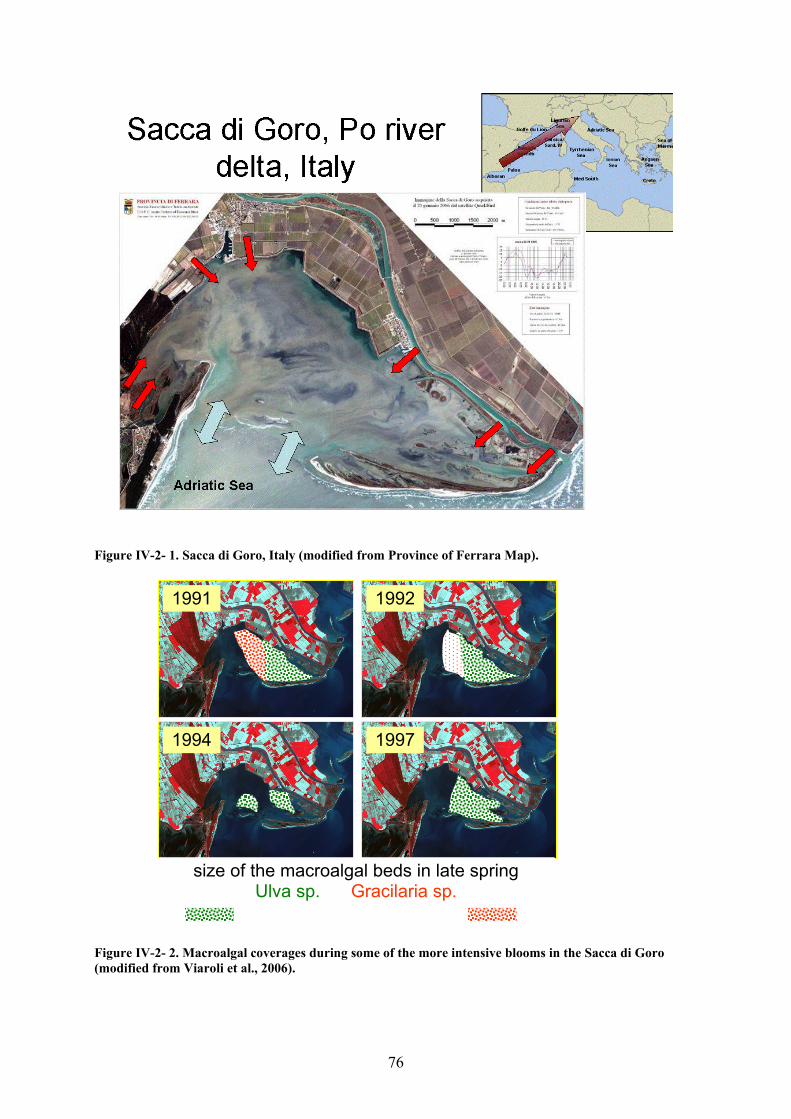
76

Figure IV-2- 1. Sacca di Goro, Italy (modified from Province of Ferrara Map).

Figure IV-2- 2. Macroalgal coverages during some of the more intensive blooms in the Sacca di Goro (modified from Viaroli et al., 2006).

1991 1992

19971994

size of the macroalgal beds in late spring Ulva sp. Gracilaria sp.

77

Figure IV-2- 3. Ulva blooms and dystrophic crisis in the Sacca di Goro in 1992 (photos of P. Viaroli).

A list of difficulties for the application of the standard LOICZ Biogeochemical model procedure to the Sacca di Goro were identified, including:

• The DIP release from the sediment due to de-adsorption processes from sediment particles (independent of P-R processes) can not be neglected.

• Redfield ratio is not appropriate in some periods as during macroalgal blooms and dystrophic crisis.

• Since it is a shallow environment (1.5 m), the sediment plays an important role in the biogeochemical cycles and the CNP ratio in the sediment is different than in the water mass.

• High concentrations of P-rich suspended solids are measured in the water column and in the water loads. The interactions with the dissolved phase are not clear and are under investigation.

• (nfix-denit) results are more negative than what we expected (<-6 mol m-2 y-1 on average), especially during the macroalgal growth phase.

Thus a slightly modified application was elaborated for the Sacca di Goro using the 0-D

biogeochemical model developed by Zaldìvar et al., 2003 (Figure IV-2-4). The model considers nutrient cycles in the water column as well as in the sediments. Furthermore, phytoplankton, zooplankton, Ulva sp. dynamics and shellfish farming are taken into account. Nutrients from the watershed, wet and dry deposition, temperature, light intensity, wind speed and shellfish production are considered as forcing functions.

Benthic fluxes of oxygen and nutrients are estimated for the 1989-98 decade with this model

(Figure IV-2-5). The results are compared with in situ measurements conducted in a series of stations in 1991, 92 and 97. The large data variability observed in these data can be ascribed to the method used (incubation period, core diameter,…), light conditions (light, dark) and stations’ characteristics (freshwater influence, benthic diatoms colonisation…). Thus, it’s very difficult to obtain flux estimations relative to the whole lagoon from in situ measurements but we can see that the model results are in the range of these measured data. Further validations of the model were conducted by Zaldivar et al., 2003.

macroalgal bloommacroalgal bloom dystrophic crisisdystrophic crisis

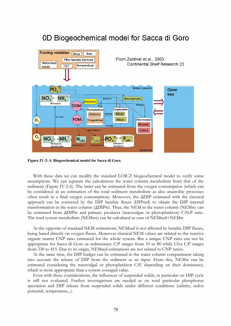
78

Figure IV-2- 4. Biogeochemical model for Sacca di Goro.

With these data we can modify the standard LOICZ biogeochemical model to verify some assumptions. We can separate the calculations the water column metabolism from that of the sediment (Figure IV-2-6). The latter can be estimated from the oxygen consumption (which can be considered as an estimation of the total sediment metabolism as also anaerobic processes often result in a final oxygen consumption). Moreover, the ΔDIP estimated with the classical approach can be corrected by the DIP benthic fluxes (DIPsed) to obtain the DIP internal transformation in the water column (ΔDIPw). Thus, the NEM in the water column (NEMw) can be estimated from ΔDIPw and primary producer (macroalgae or phytoplankton) C:N:P ratio. The total system metabolism (NEMws) can be calculated as sum of NEMsed+NEMw.

At the opposite of standard NEM estimations, NEMsed is not affected by benthic DIP fluxes,

being based directly on oxygen fluxes. Moreover classical NEM values are related to the reactive organic matter CNP ratio estimated for the whole system. But a unique CNP ratio can not be appropriate for Sacca di Goro as sedimentary C:P ranges from 10 to 80 while Ulva C:P ranges from 330 to 415. Due to its origin, NEMsed estimations are not related to CNP ratios.

At the same time, the DIP budget can be estimated in the water column compartment taking into account the release of DIP from the sediment as an input. From this, NEMw can be estimated considering the macroalgal or phytoplankton C:P, depending on their dominance, which is more appropriate than a system averaged value.

Even with these considerations, the influences of suspended solids, in particular on DIP cycle is still not evaluated. Further investigations are needed as on total particular phosphorus speciation and DIP release from suspended solids under different conditions (salinity, redox potential, temperature,..).

79

Due to these considerations, NEMws, which is the sum between NEMsed and NEMw, should be more appropriate in catching the metabolism evolution of the system than the traditional NEM.

Figure IV-2-7 shows the seasonal evolution of NEM and NEMws along with the Ulva

biomass measured in a critical station of the lagoon (st.17). Note the differences in the temporal steps among NEM and biomass values. The first series average 3 months data while for the latter single measured values are reported. Both NEM and NEMws follow the seasonal evolution of macroalgal blooms as they are positive during the growth season (high production) and negative in the decay seasons (high respiration). NEMws is generally more positive than NEM because of the assumptions described before; this is particularly true during the dystrophic crisis due to large releases of DIP from PO4 adsorbed to sediment particles.

Figure IV-2- 5. Comparison between model based estimates of benthic fluxes and observations in the Sacca di Goro (modified from Giordani et al., 2008).

80

Figure IV-2- 6. Some proposed modifications to the LOICZ methodology in the Sacca di Goro.

Figure IV-2- 7. Estimates of Net Ecosystem Metabolism in the Sacca di Goro (modified from Giordani et al., 2008).

81

The assumptions described above have little effect on the DIN cycle as (nfix-denit) is similar to (nfix-denit)ws. Too high negative values of (nfix-denit), which is the difference between ΔDIN and ΔDINexp, are estimated and due to high negative values of ΔDIN (-7.5 mol m-2 y-1 as average of the whole period). This is due to the large inputs from the channels and from the Adriatic Sea which is affected by the Po river plume that extends in front of the lagoon and often shows high DIN concentrations. Considering these large inputs and DIN concentrations, ΔDIN is too negative in comparision to ΔDINexp indicating that an important sink of DIN is missing or some flux estimations are erroneous. But since the (nfix-denit) peaks are related to the macroalgal blooms, a significant role can be played by these nitrophilous plants as an extra nitrogen storage (luxury uptake). Further investigations are needed.

Figure IV-2- 8. Nitrogen dynamics in the Sacca di Goro (modified from Giordani et al., 2008).

In conclusion, the proposed modification of the LOICZ budget approach appears to be giving more consistent estimations of the Sacca di Goro metabolism but it can hardly be applied to other systems due to the large number of data and models (as 0D model) required. Further investigations are needed to assess the role of suspended solids and macroalgae on DIP and DIN budgets.

82

3. LOICZ BUDGET METHODOLOGY REVIEW

Fred Gazeau


In the last few years and in the framework of the EUROTROPH project (Contract

#EVK3-CT-2000-00040; http://www.co2.ulg.ac.be/eurotroph/ ), we made use of the LOICZ budget methodology to assess the metabolic balance of several coastal ecosystems: the Randers Fjord (Denmark), the Scheldt estuary (Belgium/The Netherlands) and the Scheldt plume. Those studies have been published in peer-reviewed journals:

1) Gazeau, F., A. V. Borges, C. Barrón, C. M. Duarte, N. Iversen, J. J. Middelburg, B. Delille, M.-D. Pizay, M. Frankignoulle and J.-P. Gattuso (2005). "Net ecosystem metabolism in a micro-tidal estuary (Randers Fjord, Denmark): evaluation of methods." Marine Ecology Progress Series 301: 23-41.

2) Gazeau, F., J.-P. Gattuso, J. J. Middelburg, N. Brion, L.-S. Schiettecatte, M.

Frankignoulle and A. V. Borges (2005). "Planktonic and whole system metabolism in a nutrient-rich estuary (the Scheldt Estuary)." Estuaries 28(6): 868-883.

3) Schiettecatte, L.-S., F. Gazeau, C. van der Zee, N. Brion and A. V. Borges (2006).

"Times series of the partial pressure of carbon dioxide (2001-2004) and preliminary inorganic carbon budget in the Scheldt plume (Belgian coastal waters)." Geochemistry Geophysics Geosystems 7(6): Q06009, doi:10.1029/2005GC001161.

1) In the first paper, we compared net ecosystem production (NEP; p-r in the LOICZ terminology) estimates during two field campaigns, based on the LOICZ method with those obtained from the use of several other techniques: the classical oxygen incubation method (both planktonic and benthic), dissolved inorganic carbon budgets based on the apparent zero end-member method and the Response Surface Difference method based on diel oxygen changes. Most of the time, all methods provided consistent estimates both in sign and magnitude. However, we also highlighted some limitations and uncertainties regarding all methods used. For instance, during the first cruise, the LOICZ method gave slightly different estimates of NEP than the other methods. This overestimation could have several causes. Nevertheless, we highlighted that in this system dissolved organic compounds cycling can play a non-negligible role. Indeed, dissolved organic nitrogen has been shown to serve as an important nitrogen source in this estuary (Veuger, B., J. J. Middelburg, H. T. S. Boschker, J. Nieuwenhuize, P. van Rijswijk, E. J. Rochelle-Newall and N. Navarro (2004). "Microbial uptake of dissolved organic and inorganic nitrogen in Randers Fjord." Estuarine Coastal and Shelf Science 61(3): 507-515.). Most budgets using the LOICZ procedure consider dissolved organic phosphorus (DOP) cycling as negligible which, in our idea, can lead to slight errors in the NEP computations. In this paper, we also highlighted a problem related to the conversion of dissolved inorganic phosphorus (DIP) non-conservative fluxes to carbon units. The studied system was a very shallow estuary (mean depth: 1.6 m) and the benthic compartment was very active in terms of primary production and organic matter mineralization (based on the O2 incubations). Thus, the use of a classical Redfield ratio was quite problematic. As we didn’t have information on a ratio we could use for this system, this may have led to an

83

additional error in the computations. Anyway, using a C:P ratio of 195:1 for benthic algae (far above the phytoplanktonic Redfield ratio) did not lead to a significant change in our results. In summary, although some limitations have been highlighted such as the importance of DOP cycling, the LOICZ procedure has revealed to be very useful to estimate the metabolic balance of this estuary as it is based on parameters easy to gather and is much less time-consuming that more “classical” methods such as bottle and/or sediment core incubations. A table summarizing the advantages and weaknesses of the different methods used in this study can be found on Table 9 of this paper. 2) In this paper, we compared, over an annual cycle, NEP estimates based on the LOICZ method (applied both on DIP and dissolved inorganic carbon, DIC) and on oxygen incubations. The Scheldt estuary is a turbid macro-tidal estuary located in Belgium and The Netherlands. This estuary has revealed to be a perfect example where the LOICZ method based on DIP cannot be applied. Indeed, suspended particulate matter (SPM) concentrations are usually higher than 50 mg/L. Therefore, processes of sorption/desorption to and from SPM play an important role in DIP cycling. It has been estimated that these abiotic non-conservative DIP fluxes account for more than 50% of the total non-conservative fluxes in the inner estuary preventing this method to give realistic estimates in this system. An also important feature of this study was the use of the LOICZ procedure applied to DIC. This procedure is attractive as, of course, it allows NEP computations directly in carbon units without the use of conversion factors. Nevertheless, this procedure has two prerequisites: first, one needs to make sure that calcium carbonate cycling is negligible in the considered system (which was a priori the case in the Scheldt estuary) or to estimate the non-conservative fluxes of DIC due to net calcification and consider it in the NEP computations; second as air-sea fluxes account for a significant part of DIC variations, they need to be accurately estimated. This is actually the second point that we focused on in this paper. The flux of a gas at the air-sea interface depends on: 1) the solubility of the considered gas (dependent on temperature and salinity), 2) the gradient of the gas at the interface and 3) the gas transfer velocity also called piston velocity which is most of the time estimated based on wind speed data. Using a general equation is quite problematic as we have shown that the gas transfer velocity is site-specific (Borges, A. V., B. Delille, L.-S. Schiettecatte, F. Gazeau, G. Abril and M. Frankignoulle (2004). "Gas transfer velocities of CO2 in three European estuaries (Randers Fjord, Scheldt and Thames)." Limnology and Oceanography 49(5): 1630-1641.). In the present paper, we have shown that using the Raymond and Cole (2001) relationship based on a compilation in various estuaries (Raymond, P. A. and J. J. Cole (2001). "Gas exchange in rivers and estuaries: choosing a gas transfer velocity." Estuaries 24(2): 312-317.), and a relationship established for the Scheldt estuary linking the gas transfer velocity to wind speed but also water currents (Borges, A. V., J. P. Vanderborght, L. S. Schiettecatte, F. Gazeau, S. Ferron-Smith, B. Delille and M. Frankignoulle (2004). "Variability of the gas transfer velocity of CO2 in a macrotidal estuary (the Scheldt)." Estuaries 27(4): 593-603.), leads to strong changes in the computed NEP value. A comparison between the LOICZ budgeting procedure and the O2 incubation method revealed strong discrepancies which were hard to fully understand as both methods were clearly subjected to strong uncertainties. 3) In this paper, we made use of the LOICZ budgeting procedure applied to DIP to compute NEP in the Scheldt estuarine plume. The budget failed to provide NEP estimates consistent with the pCO2 dynamics in this area, especially in spring when computed NEP values are clearly too low to explain the observed decrease of pCO2 during that period. This discrepancy has been attributed, at least partly, to a physiological property of the dominant phytoplanktonic species in that period in the Scheldt plume: Phaeocystis sp. Indeed, this species has the ability to grow, under DIP depleted conditions, on DOP by means of the alkaline phosphatase (AP). Therefore, as we have shown for the Randers Fjord in spring, the present study highlights another problem

84

associated with the use of the LOICZ budgeting procedure applied to DIP for a system dominated by a potentially DOP-growing species. Conclusions and additional remarks

The LOICZ budget methodology is a very useful tool for assessing the metabolic balance of coastal ecosystems as 1) it requires parameters which are routinely measured in many coastal sites, 2) allow estimates on both large temporal and spatial scales and 3) easy to implement. Nevertheless, as many other methods, it has its own associated limitations and uncertainties:

1) Conservative fluxes (water and salt budgets) cannot be accurately assessed if the salinity gradient is too small as it will induce considerable errors in the final computed rates. This was actually the case in one of our study site, the Bay of Palma (Mallorca, Spain), where freshwater inputs and residence times are too low to create a sufficient salinity gradient, preventing the use of this procedure.

2) In relatively large systems bordered by cities and/or agricultural areas, such as the Scheldt estuary for instance, lateral fluxes have to be considered. These fluxes are most of the time difficult to estimate and will of course be dependent on climatic conditions.

3) Preferably, the particulate organic matter C:P ratio of the considered system has to be known as large variations can be found whether the system is planktonic or benthic-dominated.

4) We highlighted some problems associated with the use of DIP to compute NEP: i) potential importance of abiotic fluxes (sorption/desorption processes) in case of a turbid system ii) importance of DOP cycling in some cases…

5) Difficulties to apply this procedure on DIC as air-sea CO2 fluxes play an important role in DIC non-conservative fluxes and are difficult to accurately estimate.

As long as these potential problems are carefully evaluated, the LOICZ budget methodology is an invaluable tool for management purposes in the coastal zone. For instance, although these results have not been published yet, we applied this method over a 10-year period in the Randers Fjord which allowed highlighting a significant increase of NEP rates which can be related to the important regulatory measures implemented in this area since the 1970’s. Improvements: As most of the time, variables used to compute LOICZ budgets are time and/or spatial averages, in each of the 3 studies cited above, we carefully performed error analyses on our budgets by using a Monte-Carlo procedure. It would be really useful, in the future, for someone who wants to make use of a LOICZ budget to develop a program which allows the implementation of such budget in any conditions (multi-box and multi-layer budgets; equivalent to the Cabaret software) but also allows performing a careful error analysis. This tool should be computed using a program available on every operating platforms (such as R for instance).

85

4. LINKING WATERSHED-BASED NANI MASS BALANCE MODEL WITH THE COASTAL LOICZ BUDGETS

Haejin Han

University of Michigan, School of Natural Resources and Environment, Dana Building, 440 Church Street, Ann Arbor Michigan 48109-1041. Email:

[email protected] Considering the stream-river-lake-estuary-ocean hydrosphere continuum, excess nitrogen

lost from terrestrial ecosystems and transported through lake and river ecosystems eventually reaches estuaries, accelerating eutrophication and anoxia in coastal ecosystems. Thus, to better understand nitrogen delivery from land to coastal area to ocean and thus potential management intervention opportunities, many investigators have utilized a “Budget model of nutrients (C, N, and P)”, a simple mass balance calculation of nutrients, for a variety of systems ranging from a soil compartment to a watershed to a coastal or lake water body.

Many of these studies have developed anthropogenic and/or natural nitrogen (N) budgets at the watershed scale, estimating nitrogen loading to landmass and the subsequent riverine nitrogen flux to lakes and coastal areas and finally examining the relationship between those watershed nitrogen inputs and riverine nitrogen exports. Among numerous watershed-based nitrogen mass balance approaches, a net anthropogenic nitrogen input (NANI) budget put forth by Howarth et al. (1996) has been the most well-known nitrogen budgeting method, and applied to various watersheds across a variety of temporal and spatial scales (North Atlantic Ocean, Howarth et al. (1996); coterminous United States, Jordan and Weller (1996); large river basins of Northeastern U.S., Boyer et al. (2002); small watersheds of Illinois, David and Gentry (2000)). Here, NANI is the sum of fertilizer use, nitrogen fixation in agro-ecosystems, the net import of nitrogen in human food and animal feed, and the atmospheric nitrogen deposition. Most of these studies find a high correlation between NANI and riverine nitrogen exports across a wide range of spatial settings, and a substantial excess of anthropogenic nitrogen inputs relative to riverine export (Van Breemen et al. 2002).

On the other hand, other research groups such as the land-ocean interactions in the coastal zone (LOICZ) working groups have constructed nutrient budget models for a coastal water body, as the system of interest, from coastal lagoons to individual shelf seas, to describe the change in coastal marine environment along the gradient of change in anthropogenic pressures, changes which are sensitive to both flushing intensity (and thus coastal hydrological inputs) and nutrient loadings.

The link of the watershed based NANI model with the LOICZ costal budget can provide two different advantages, as described below. First, the combined land-coastal budgets help addressing key issues of coastal change and use in the context of scenarios of future human activities and climate change. An important application of NANI models that predict nitrogen export from rivers is the forecasting of future riverine nitrogen exports, based on likely scenarios of future nitrogen inputs that take into account changes in farming practices, agricultural production systems, and predicted climate change (Howarth et al. 2002, Howarth et al. 2006). For instance, based on various assumptions and models, Howarth et al. (2002) forecast riverine TN exports from the entire U.S. for the year 2030 by exploiting the predicted future NANI in 2030 based on the conservative status quo scenario and the identified spatial relationship between NANI and riverine nitrogen exports from large regions, (i.e., on average 25% of total NANI to the landscape is transported to rivers). In another application, Howarth et al. (2006) predicted future riverine TN exports for the Susquehanna River in the northeastern United States, incorporating both NANI and future climate change but assuming that NANI simply remains

86

constant into the future. Using the projected future riverine nitrogen exports based on a variety of scenarios of future human activities in terms of land use, farming practice, and human dietary habits, the LOICZ budget can forecast how land-oriented nitrogen in-flux in future will affect the nitrogen budgets of the coastal zone and in turn, can develop scenarios that investigate the implications of these changes on human society.

Second, the NANI model can permit us to extrapolate nitrogen river flux estimates, which is an input flux of the coastal budget, from a set of well-monitored rivers to unmonitored rivers based on the identified relationship between NANI and riverine TN exports across the monitored watersheds. Many previous NANI studies have successfully shown that either spatial or temporal variation in river nitrogen export can largely be explained as a function of nitrogen sources, in spite of the large variation in nitrogen controlling processes that likely occur in watersheds across various spatial and temporal scales (Howarth et al. 1996, Jordan and Weller 1996, Burkart and James 1999, David and Gentry 2000, Goolsby et al. 2000, 2001, Boyer et al. 2002). In addition, compared with availability of data on river chemistry observations for the rivers of the world, a global database used to estimate nitrogen inputs to continental landmass are more easily to be obtained. Some recent studies have already provided biophysical data sets used for accounting of mass balance of nitrogen inputs at the global scale including all major agricultural input (fixation, and fertilizer), atmospheric input and output, and human and livestock population (Dentener and Crutzen 1994, Galloway et al. 2003, Green et al. 2004, Van Drecht et al. 2005). As a result, the NANI approach is likely to provide a helpful way to extrapolate the flux calculations from budgeted regions of the coastal zone to unbudgeted regions using accepted statistical procedures and the forecasted riverine TN exports from NANI model in order to improve our understanding of material fluxes to and from the coastal zone of the world’s oceans.

1. Net anthropogenic nitrogen input (NANI) budgets Most of these studies find a high correlation between net nitrogen inputs and riverine

nitrogen exports across a wide range of spatial settings, and a substantial excess of anthropogenic nitrogen inputs relative to riverine export (Van Breemen et al. 2002). However, such studies also agree that estimates of net nitrogen input terms contain considerable uncertainty and errors, because estimates of nitrogen sources, losses, and the net nitrogen input balance can vary widely depending on the definition of the system boundary, the assumptions and approximations used to estimate nitrogen flows, and on the quantity and quality of available data over space and time. Recently, Han (2007) suggested that relationships between watershed nutrient inputs and riverine exports were improved, especially for small watersheds with diverse land use and farming practices, in response to specific model adjustments, by comparing the performance of nine alternative NANI models for predicting riverine TN exports. For example, NANI estimation procedures that accounted for seasonal fluctuations in livestock populations, and estimated crop nitrogen fixation using crop yield methods rather than area harvested, resulted in stronger models (Han 2007). In addition, this study also demonstrated the identified spatial relationship between inputs and exports vary by year as a function of annual water discharge. Therefore, it is needed to develop reliable relationships between NANI and riverine nitrogen exports across major river basins across the world, using 1) the exactly same NANI methods based on the same system boundary (e.g. watershed scale, or soil compartment), 2) fixed numbers and types of nitrogen input and output terms, 3) consistently defined geographic spatial scales and periods and 4) incorporating more detailed information on agricultural farming practice.

Estimation of NANI requires a number of databases from a variety of sources, as summarized in Table 1. NANI estimation relies heavily on agricultural statistics, because most nitrogen input terms are highly associated with agricultural activities. Thus it is important to select the most reliable agricultural databases with appropriate spatial and temporal resolution of

87

data. Although North America, Europe and many countries in other regions have good statistics on agricultural nitrogen and phosphorus use, the availability of agricultural statistics is not uniformly available for all parts of the globe. Thus, there are crucial needs to select the proper spatial scales with the adequate data sets for NANI budgets as well as to elaborate the methods to aggregate county-wide or regional-wide agricultural statistics to the smaller unit of watershed.

88

Tab

le I

V-

1. A

gric

ult

ura

l sta

tist

ics

use

d t

o es

tim

ate

NA

NI

(ad

apte

d f

rom

Han

, 200

7 fo

r th

e U

S a

nd

Gre

en

et a

l., 2

004)

.

Sp

atia

l un

it

Sou

rce

Sp

atia

l un

it

Lit

erat

ure

s so

urc

ena

tion

alU

SD

Aco

unty

US

GS

1km

, cou

ntry

sta

tist

ics

ED

C (

2000

), F

AO

(200

1)st

ate

Fert

iliz

er

Wet

dep

osit

ion

of in

orga

nic

N25

00×

2500

m

ete r

NA

DP

/NT

N

Dry

dep

osit

ion

of in

orga

nic

N25

00×

250

0 m

eter

CA

ST

NE

T

Nat

iona

l em

issi

on o

f N

Ox

nati

onal

EP

A

nati

onal

Van

Aar

denn

e et

al

. co

untr

y st

atis

tics

Van

Aar

denn

e et

al.

nati

onal

EP

AN

et im

port

of

Nin

foo

d an

d fe

ed

Pop

ulat

ion

coun

ty /s

tate

U.S

. Cen

sus

Bur

eau

1km

, cou

ntry

sta

tist

ics

Vör

ösm

arty

et a

l. (2

000)

, FA

O(2

001)

Cro

p ac

reag

eco

unty

US

DA

/1k

m, c

ount

ry s

tati

stic

sE

DC

(20

00),

FA

O(2

001)

NR

CS

g

Sta

te S

oil

Geo

grap

hic

(ST

AT

SG

O)

grid

EP

Agr

idU

SG

S

Uni

ted

Sta

tes

(Han

(20

07))

Glo

bal d

ata

set (

adap

ted

from

Gre

en e

t al.

(200

4))

5 °

Den

tene

r et

al.

(199

4)

1 °,

cou

nty

stat

isti

csL

erne

r et

al.

(198

9), F

AO

(200

1)

Cro

p in

vent

ory

coun

tyU

SD

A/N

AS

S

Bio

logi

cal N

fi

xati

onS

oil m

ap (

ST

AT

SG

O)

1:25

0,00

0

Lan

d us

e

Atm

osph

eric

N

depo

siti

on

Nat

iona

l em

issi

on o

f N

Hy

Ani

mal

inve

ntor

y an

d sa

les

coun

tyU

SD

A/N

AS

S

Cat

egor

yD

ata

typ

e

N F

erti

lize

rN

fer

tili

zer

sale

89

5. TWO POSSIBLE POINTS OF INTERSECTION FOR LOICZ AND ITS MISSION TO INFORM SUSTAINABLE DEVELOPMENT: FISHERIES AND ECOLOGICAL ECONOMICS.

Karin E. Limburg

State University of New York, College of Environmental Science & Forestry

Syracuse, NY 13210 USA. Email: [email protected]

As LOICZ moves into Phase 2, and begins implementing its programs to inform and support sustainable development initiatives in coastal zones, two topic areas are likely to become important foci for LOICZ’s research and capacity building. The first is fish and fisheries, and the second is a suite of socio-economic alternative (“heterodox”) paradigms, typified by ecological economics.

Fish and fisheries.

Worldwide, fisheries are in crisis, particularly the marine and diadromous species. The FAO’s latest State of the World’s Fisheries and Aquaculture (FAO 2006) reports that 52% of global marine fish stocks are fully exploited, and another 25% are overexploited (overfished), depleted (collapsed), or recovering (closed). The causes are many, but in general include overfishing (including unreported bycatch), habitat loss, and in some cases, pollution. Habitat loss includes not only marine areas (coastal and otherwise), but also within-continent habitats for the diadromous species. In the latter case, urbanization and dams have caused extensive fragmentation and alteration of key spawning and nursery areas. This is all very well documented, albeit rarely pulled together in a synthetic manner (Helfman, 2007).

The case of pollution and fisheries poses an interesting possible nexus of fisheries with the nutrient budgeting activities of LOICZ. For some time now, researchers have pointed out the “fertilization effect” of nutrient loading on fisheries, with observations, at coarse spatial scales, of a positive correlation of fisheries landings and primary production and/or nutrient loading (Oglesby 1977; Nixon 1988; Downing et al. 1990). In some cases (e.g., Cederwall and Elmgren 1980), faunal biomass increases have been documented. However, there is also evidence of fisheries declines, or changes in the mix of pelagic and demersal species, as nutrient loading increases beyond some point (Caddy 1993, 2000). This pattern needs further investigation and documentation (see Hondorp et al. 2007), and the mechanisms are unclear at this point. However, the LOICZ database could be put to very good use to examine and further define (or refute) this relationship, and could also be used to pose and test hypotheses about the relationship. For example, is the relationship a direct effect, perhaps of toxic levels of nitrates and/or ammonium, or the occurrence of hypoxic or anoxic conditions? Or is the cause indirect due to habitat loss, caused by the “polluto-succession” of seagrasses losing out to macroalgae, which eventually are out-competed by phytoplankton (e.g., Duarte 1995)? The LOICZ database could be combined with other data to examine these hypotheses, and in addition, examine whether particular land-ocean configurations are more or less susceptible to producing hypereutrophic (or “dystrophic”) conditions.

Some specific recommendations for incorporating fisheries considerations into LOICZ phase II:

• Convene a workshop specifically to identify linkages between fisheries and watersheds. This workshop could be sub-divided into several parts, for instance,

90

• Nutrient fluxes and fisheries

• Eutrophication effects on fisheries

• Land-use effects on fisheries

• Alterations of in-stream and riparian features on fisheries (e.g., dams, development)

• Management recommendations.

• Produce a peer-reviewed report that can be widely disseminated.

Ecological Economics.

Conventional economics provides the current prevailing framework in which most human activities are valued and monetized for purposes of trade and other exchanges. However, there are well-known circumstances under which conventional paradigms fail to impute value, leading to problems in equity (e.g., the under- or non-valuation of women’s labor), distribution (e.g., the loss of jobs to foreign shores), and resource allocation. Ecological economics is a relatively new field that tries to address all these aspects, but especially is concerned with the interface of natural and human systems. Ecological economics is grounded in thermodynamics and therefore, unlike conventional (neoclassical) economics, identifies strict constraints on use of biophysical resources.

The “three pillars” of ecological economics are sustainable scale, equitability, and efficient allocation (Costanza et al. 1997). Conventional economics deals mainly with this last point, and not at all with the first. Rather, as put by Gowdy (1997), neoclassical theory embraces an “everything-is-substitutable, everything-has-a-price world (p. 32).” In contrast, ecological economics recognizes that ecosystems often produce goods and services that are not substitutable (e.g., particular species, habitats, or context-specific functions), and that much of these do not have a clear price. A final point of departure of ecological economics from the conventional paradigm is the vision of humanity and its enterprises as a subset of the biosphere; by contrast, conventional economics regards Nature as a set of inputs into the “main” system, the economy.

Although the field of ecological economics is broad, and overlaps with that of environmental economics (a subset, in turn, of microeconomic theory), one major thrust of ecological economics is the identification, quantification, and valuation of ecosystem goods and services. These may be defined as the stocks and flows of materials, as well as functions, derived from ecosystems that support humans (Daily 1997). The Millennium Ecosystem Assessment comprehensively details global trends in ecosystems and their ability to provide ecosystem services (Millennium Ecosystem Assessment 2005).

As LOICZ phase II moves ahead, ecosystem service identification, quantification, and possibly valuation within watersheds and associated coastal zones may prove to be a useful and valuable project. A literature is developing on methods, but to date there are few, if any, standard methodologies available, and many ad-hoc ones. A number of general methods may be found in ecological economics textbooks (e.g., Costanza et al. 1997; Daily 1997; Common and Stagl 2005; Farley et al. 2005), journal articles, and even websites (www.ecosystem valuation.org). Many methods are criticized for having weaknesses, and some of these have to do with underlying assumptions, philosophies, or both.

91

Some specific recommendations for incorporating ecological economics approaches into LOICZ phase II:

• Convene a workshop (or workshops) to identify and develop standardized methodologies for ecosystem services quantification and valuation in the coastal zone (LOICZ-relevant areas)

• Produce a website with downloadable methodologies, similar to what was done for LOICZ phase I nutrient budgeting

• Provide funds (small grants?) for researchers to develop site-specific, ecosystem service quantification and valuation in areas relevant to the LOICZ mission (e.g., coastal ecosystems and their associated watersheds)

• Provide a clearing-house of reviewers of these and other valuation exercises;

Produce a web-based database of the above, with links to other related efforts.

92

6. THE “SWEET SPOT”: NOTES ON APPLYING CLASSICAL OXYGEN-SAG MODEL APPROACHES TO HYPOXIA IN THE GULF OF MEXICO AND THE

CHESAPEAKE BAY*

Don Scavia University of Michigan, Graham Sustainability Institute, 625 E. Liberty Rd., Ann Arbor Michigan 48104; Email: [email protected]

Figure IV-6. 1. The Streeter-Phelps equation provides a compelling example of a relatively simple, classic engineering model designed to estimate the response of oxygen levels to pollution in a river. With few modifications, the model can be used as a simple screening or planning tool to address the problem of hypoxia associated with riverine and estuarine nutrient loads. Examples of hypoxia in the Gulf of Mexico and Chesapeake Bay are discussed below (figure courtesy of D. Scavia). *Notes on slides compiled by Dennis Swaney.

93

Figure IV-6. 2. Streeter-Phelps model equations include terms for advective transport, biological breakdown, and reaeration terms. Separate equations are written for BOD (biological oxygen demand) and dissolved oxygen (DO) deficit, ie the difference between oxygen concentration at its saturated value and the actual value in the water column (figure courtesy of D. Scavia).

Figure IV-6. 3. The solution to the dissolved oxygen equation yields a characteristic “sag curve” predicting a DO minimum downstream of each source of BOD (figure courtesy of D. Scavia).

94

Figure IV-6. 4. BOD loads can be related to nitrogen loads feeding production of excessive organic matter decay. In the Gulf of Mexico, separate sources can be attributed to the Mississippi and the Atchafalaya(figure courtesy of D. Scavia). Figure IV-6. 5. The “hypoxic patch” or “plume” associated with the combined nutrient loads can be defined as the extent of the downstream oxygen profile falling below the DO threshold (here, hypoxia is set at 3 mgL-1). Depending upon the magnitude of combined loads, no hypoxic patch may occur, or one or two patches could occur (figure courtesy of D. Scavia).

95

Figure IV-6. 6. The oxygen sag model was originally developed as a 1-dimensional model, and the “patch length” is defined along the longitudinal axis. However, empirical observations of the hypoxic areas show that the area of the patch is directly related to its length (most variation is along its axis) (figure courtesy of D. Scavia). Figure IV-6. 7. The variation of observed patch length and area over several years can be used to calibrate the model (estimate model parameters so that the model best fits the observations). Once the model is calibrated, it can be used to predict future extent of hypoxia in terms of load and other environmental variables (figure courtesy of D. Scavia).

96

Figure IV-6. 8. The model can also be used to examine the response of the hypoxic areas to a range of nutrient load scenarios. Repeating the analysis over a likely range of environmental variables (an “ensemble”) allows an ensemble forecast of hypoxic areas corresponding to range of loads, or a range of load reductions necessary to meet a desired level of hypoxic area (figure courtesy of D. Scavia). Figure IV-6. 9. Observed oxygen levels for a sampling cruise along a Chesapeake Bay transect from the riverine boundary (left) the ocean (right). Estuarine circulation in the bay means that surface layers move seaward (left to right) and deep layers move landward. . The deeper layers tend to be those subject to hypoxia. Mixing occurs between surface and deep layers (figure courtesy of D. Scavia).

97

Figure IV-6. 10. For the Chesapeake Bay, the nitrogen load is mainly supplied by the Susquehanna river. Oxygen in the deep layer below the pycnocline is considered to be a balance between mixing of oxygen from the surface layer, oxygen consumption due to organic matter decomposition in the deep layer, and landward advective transport. The schematic diagram corresponds to the circulation features in the previous figure (figure courtesy of D. Scavia). Figure IV-6. 11. As in the previous example, the observed volume of the hypoxic plume is strongly correlated to the estimated length of the hypoxic zone (figure courtesy of D. Scavia).

98

Figure IV-6. 12. As in the Gulf example, the Chesapeake model can be calibrated and compared to observed longitudinal oxygen profiles. The figure shows generally good agreement between the calibrated curve and observations (figure courtesy of D. Scavia). Figure IV-6. 13. The model can again be used with statistical tools (Monte Carlo analysis) to estimate the likely range of hypoxic volume (km3) associated with different nitrogen loading rates, together with the variability associated with natural environmental variation. Here, hypoxic volume is shown on the y axis and nitrogen load on the x axis (figure courtesy of D. Scavia). This simple modelling approach has been applied successfully in the Gulf and Chesapeake ( www.snre.umich.edu/scavia/hypoxia-forecasts/). See also Scavia and Donnelly, 2007; Stow and Scavia, 2009; Liu and Scavia, 2010, among others.

99

7. SQUEEZEBOX: A TOOL FOR CREATING FLOW-SCALED 1-D BOX MODELS OF RIVERINE ESTUARIES

Joan E. Sheldon and Merryl Alber

Dept. of Marine Sciences, University of Georgia, Athens, GA 30602 Presented by J. Sheldon at the LOICZ Budget Workshop,

Providence, RI, Nov 9-10, 2007

Introduction SqueezeBox is a desktop modeling tool that can be used to evaluate the effects of freshwater inflow on the salinity distribution and mixing time scales of riverine estuaries. Salinity is a master variable that affects many estuarine characteristics and is important to estuarine organisms. Mixing time scales, such as residence time and flushing time, provide information on water movement that can be compared with the rates of processes that may act upon materials (such as nutrients or pollutants) as they are carried through the estuary (see Sheldon and Alber (2002) for a description of the mixing time scales discussed here). Box models are often developed to calculate, for a constant river flow rate, the expected steady-state distribution throughout the estuary of a substance that mixes conservatively with water. If the goal of the modeling effort is calculation of steady-state concentrations or individual box residence times, box boundaries may be placed arbitrarily (Officer 1980), and it may seem desirable to place them at even intervals or at natural geographic features. Simulations, such as those required to calculate many mixing time scales, place additional constraints on the box sizes and time steps. Flow through a box during a time step (throughflow) must not exceed the volume of the box (i.e. the time step should meet the Courant–Friedrichs–Lewy criterion for computational stability), nor should the time step be so small as to cause significant accumulation of numerical errors. In order to avoid both these problems, Miller and McPherson (1991) recommended that the ratio of throughflow to box volume be between 0.2 and 0.5. For a given river flow, the ratio may be controlled by changing box sizes, the time step, or a combination of the two. Changing box sizes will have a direct impact on the spatial resolution of the model, whereas changing the time step will affect the temporal resolution as well as model run time. Moreover, different flows will require different box boundaries or time steps in order to meet these conditions. Neither equal box volumes nor equal box lengths generally produce the desired results for riverine estuaries (Sheldon and Alber 2002). The SqueezeBox Modeling Framework SqueezeBox produces an optimal 1-D segmentation with a consistent throughflow:volume ratio throughout the estuary so that simulations of flows among boxes are numerically stable and may be used to estimate mixing time scales and track the transport of inert tracers. It is based on the method outlined by Miller and McPherson (1991), with some modifications (Sheldon and Alber 2002). It uses smoothed equations for tidally averaged cross-sectional area and net upstream flow of seawater vs. distance along the longitudinal axis of the estuary, so that boundaries may be drawn anywhere along the estuary and the characteristics of the resulting boxes (e.g. volume, salinity) may be determined. We develop an equation for cross-sectional area vs. distance by fitting polynomial functions to mid-tide-average cross-section measurements (example described below), broken into reaches if necessary so that a good fit can be obtained with low-order polynomials (Figure IV-7-1, left). SqueezeBox can choose box boundaries automatically given a freshwater inflow rate and time step size (Figure IV-7-2), but it also has an interactive mode in

100

which the user can set box boundaries, by distance or salinity, and it will advise if the throughflow:volume ratios are in the acceptable range. We assume that the salinity distribution for any given river flow is a logistic function of distance (based on data from several estuaries examined thus far) and that simple mixing of seawater and river flows can be used to predict salinity at any location. Combining these two concepts yields an equation for net upstream flow of seawater as a function of river inflow and distance along the axis (Sheldon and Alber 2002; Figure IV-7-1, right). Salinity data taken over a range of river inflow magnitudes are used to parameterize this function so that the SqueezeBox application can predict the salinity distribution for the estuary given only a river inflow value (Figure IV-7-3).

Figure IV-7- 1. Graphs of core equations for the Ogeechee River estuary module. Left: cross-sectional area is a function of distance. Right: net upstream flow of seawater is a function of distance and river flow (from Sheldon & Alber, 2002).

101

Figure IV-7- 2. SqueezeBox input parameters include predefined equations (see Figure IV-7-1) in an estuary module, freshwater inflow rate, time step size options, and boundary conditions (figure courtesy of J. Sheldon & M. Alber).

Figure IV-7- 3. SqueezeBox creates a flow-scaled 1-D box model and estimates the salinity distribution (figure courtesy of J. Sheldon & M. Alber). We have developed modules for the Altamaha and Ogeechee River estuaries (Georgia, USA) (Sheldon and Alber 2002; 2005). In each case, cross-sectional areas at 1-km intervals along the estuary axis were estimated using chart measurements (National Oceanic and Atmospheric Admin. (NOAA) or U.S. Geological Survey (USGS)) and tidal ranges interpolated between

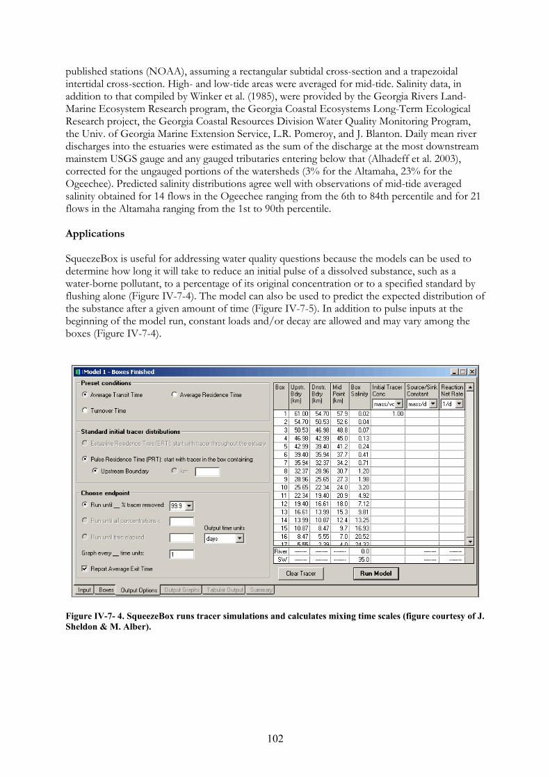
102

published stations (NOAA), assuming a rectangular subtidal cross-section and a trapezoidal intertidal cross-section. High- and low-tide areas were averaged for mid-tide. Salinity data, in addition to that compiled by Winker et al. (1985), were provided by the Georgia Rivers Land-Marine Ecosystem Research program, the Georgia Coastal Ecosystems Long-Term Ecological Research project, the Georgia Coastal Resources Division Water Quality Monitoring Program, the Univ. of Georgia Marine Extension Service, L.R. Pomeroy, and J. Blanton. Daily mean river discharges into the estuaries were estimated as the sum of the discharge at the most downstream mainstem USGS gauge and any gauged tributaries entering below that (Alhadeff et al. 2003), corrected for the ungauged portions of the watersheds (3% for the Altamaha, 23% for the Ogeechee). Predicted salinity distributions agree well with observations of mid-tide averaged salinity obtained for 14 flows in the Ogeechee ranging from the 6th to 84th percentile and for 21 flows in the Altamaha ranging from the 1st to 90th percentile. Applications SqueezeBox is useful for addressing water quality questions because the models can be used to determine how long it will take to reduce an initial pulse of a dissolved substance, such as a water-borne pollutant, to a percentage of its original concentration or to a specified standard by flushing alone (Figure IV-7-4). The model can also be used to predict the expected distribution of the substance after a given amount of time (Figure IV-7-5). In addition to pulse inputs at the beginning of the model run, constant loads and/or decay are allowed and may vary among the boxes (Figure IV-7-4).

Figure IV-7- 4. SqueezeBox runs tracer simulations and calculates mixing time scales (figure courtesy of J. Sheldon & M. Alber).

103

Figure IV-7- 5. SqueezeBox shows model tracer concentrations graphically by distance and salinity and within individual boxes and tracks total tracer mass (figure courtesy of J. Sheldon & M. Alber). Although total transit times through an estuary are useful, water that flows through a riverine estuary passes from tidal freshwater through sequentially saltier reaches, and some processes occur primarily in specific salinity zones. For example, nitrification is optimal at low to intermediate salinities (Rysgaard et al. 1999). More specific information on how long water spends within relevant reaches of the estuary would therefore allow for a better understanding of the processing of materials. Sheldon and Alber (2005) explored differences in the transit times of dissolved substances through salinity zones (tidal freshwater, oligo-mesohaline, and polyhaline) in the Altamaha and Ogeechee River estuaries under a range of flow conditions. The estuaries were compared in spite of the large difference in their river flow ranges by using flow rates ranging from the 10th-90th percentile for each river. SqueezeBox automatically generated an initial set of boxes for a given river inflow and then the interactive mode was used to adjust the boundaries slightly to match the desired salinity zones. Although the two estuaries have similar lengths and volumes, the slower-flowing Ogeechee grades from a zone of tidal freshwater (except at very low flows) through the oligo-mesohaline zones to a polyhaline zone inside the mouth whereas the Altamaha always has a longer extent of tidal freshwater but only a short (or non-existent) polyhaline zone. Transit times through the whole Ogeechee estuary are 3.3-4.7 times longer than those in the Altamaha, but the lengths of time water spends in the tidal freshwater reaches of the estuaries are comparable whereas there are large differences in the times spent in oligo-mesohaline and polyhaline reaches (Figure IV-7-6). Model responses at different river inflow levels show the value of estimating the range of an estuary’s response rather than the mean. With decreasing flow, salty water comes further upstream, the region of tidal freshwater decreases, and the extra overall transit time is spent disproportionately in saltier zones. These types of predictions may be useful in interpreting nutrient and pollutant dynamics in estuaries and in comparing the relative susceptibility of estuaries to perturbations. For example, susceptibility to excess nitrogen inputs is likely to be higher in summer when flows are generally lower, transit times longer, temperatures higher, and oxygen saturation lower.

104

Figure IV-7- 6. Lengths of salinity zones (left) and average transit times through different salinity zones of the Ogeechee and Altamaha River estuaries as a portion of the total (center) and on an absolute scale (right) for 10th-90th percentile flows for each river (Sheldon & Alber, 2005). In another study, chlorophyll a concentrations measured along the Altamaha River estuary during 10 sampling periods were compared to transit times through the entire estuary as well as through the tidal freshwater, oligohaline, mesohaline, and polyhaline zones (Sheldon and Alber unpubl.). Overall, total transit time is a good predictor of average estuary chlorophyll concentration, location of the chlorophyll peak, and salinity at the peak location. With increasing transit time, chlorophyll concentrations increase and the peak moves upstream and occurs at lower salinities. However, zone transit times can be better predictors of zone chlorophyll concentrations (Figure IV-7-7). At high flows, the tidal freshwater zone is long (>35 km) but transit time through it is very short (<1 d), and chlorophyll concentrations are nearly zero except in the lower estuary. As flows decrease, most of the extra transit time is spent in higher-salinity zones, and chlorophyll increases in these zones. Chlorophyll in tidal freshwater remains minimal until the freshwater zone transit time surpasses 1.3 d, then rises rapidly, suggesting that net phytoplankton production has overcome flushing.

D

isch

arge

(m

3 s-1

)

Segment TransitTime (d)

Portion of TotalTransit Time

Estuary SegmentLength (km)

Dis

char

ge (

m3 s

-1)

Altamaha

0% 25% 50% 75% 100%

Altamaha

0 10 20 30 40 50

92121154192240309428609933

tidal fresh oligo-mesohaline polyhaline

OgeecheeOgeechee

152332435982

116167273 Ogeechee

152332435982116167273

Altamaha

0102030405060

92121154192240309428609933

105

Figure IV-7- 7. Left column: relationships between total transit time and average chlorophyll concentration, location of the peak in chlorophyll concentration, and the low water salinity at the location of the chlorophyll peak in the Altamaha River estuary. Right: relationships between cumulative transit time through different salinity zones and average chlorophyll concentrations in those zones (figure courtesy of J. Sheldon & M. Alber). Complementarity between SqueezeBox and LOICZ budgets Currently, SqueezeBox does not incorporate the C:N:P stoichiometric calculations of the LOICZ method, but it could be a useful tool for enhancing the LOICZ methodology or providing additional information for estuaries where it is applicable (riverine estuaries that are generally well-mixed vertically and laterally). SqueezeBox is programmed in Microsoft Visual Basic and runs quickly on ordinary desktop computers. Like the LOICZ methodology, it is designed to be flexible and easily adaptable to different estuaries with minimal data requirements. The framework is modular: equations and data from external files are used to generate box models for an estuary, so new estuary modules can be incorporated without knowledge of programming. Module development requires bathymetry data, freshwater input rates, and salinity observations throughout the estuary at a range of freshwater flows. SqueezeBox models could be used to explore the seasonal and interannual variability in water and salt budgets; to supply information on flows, residence times, and conservative nutrient (Y) behavior for seasonal LOICZ budgets; and to estimate net nutrient fluxes (ΔY). Acknowledgments Funding was provided by The Nature Conservancy, the Georgia Coastal Ecosystems LTER Project (NSF OCE 99-82133), and the Georgia Coastal Management Program (NOAA NA17OZ1119).

Average Zone Chlorophyll a Concentration (µg/L)

Cumulative Zone Transit Time (d)

0

20

40

0 2 4 6 8 10

tidal fwoligomeso

Total Transit Time (d)

Average Estuary Chlorophyll a Concentration (µg/L)

Location of the Chlorophyll Peak (km)

Low Water Salinity at the Peak Location

R2 = 0.77

0

20

40

R2 = 0.92

-100

102030

R2 = 0.67

0

5

10

15

0 5 10 15

106

8. ANALYSIS OF LONG-TERM WATER QUALITY OF THE PATUXENT ESTUARY USING A MULTI-COMPARTMENT MODEL APPROACH

Jeremy Testa

University of Maryland Center for Environmental Science, Cambridge, MD. Email: [email protected]

Our recent research using multi-compartment LOICZ models to assess system responses to

changes in nutrient loading have provided unique insight and direct conclusions to both the scientific and management communities involved with the Patuxent River estuary’s water quality. The system was divided in 3 regions (upper, middle and lower estuary) and 6 boxes (Figure IV-8-1).

In this recent research, we conducted a quantitative assessment of estuarine ecosystem

responses to reduced phosphorus and nitrogen loading from sewage treatment plants and freshwater inputs variability to the Patuxent River estuary (Figure IV-8-2). We analyzed a 19-year data set of water quality conditions, nutrient loading, and climatic forcing for 3 estuarine regions. We also computed monthly rates of net production of dissolved O2 and physical transport of dissolved inorganic nitrogen (DIN) using a two-layered salt- and water-balance model. Point source loading of DIN and DIP to the estuary declined by 40-60% following sewage treatment plants upgrades (BNR: Biological Nutrient Removal) and correlated with decreasing DIN and DIP concentrations throughout the Patuxent River (Figure IV-8-2, 3). Reduced nutrient loading and concentration resulted in non-significant declines in primary productivity, Chl-a, and bottom layer O2 consumption in the upper regions of the estuary (Figure IV-8-4, upper panel). Despite significant reductions in seaward nitrogen transport to the middle and lower estuary, Chl-a and surface-layer net O2 production have actually increased while water clarity has decreased, especially during summer (Figure IV-8-4, middle and lower panels). This degradation of water quality appears to be linked to increasing net inputs of DIN into the estuary from Chesapeake Bay, as calculated from box-model-computed nutrient transport rates (Figure IV-8-5). Indeed, summer Chl-a and annual net O2 production in the lower estuary correlate significantly with the net import of DIN from Chesapeake Bay (Figure IV-8-6). These results underscore the need for parallel abatement of nutrient loads to both Chesapeake Bay and its tributaries.

Hypoxia develops in the middle region of the Patuxent estuary each year and hypoxic

volume did not diminish with reduced nutrient inputs from sewage treatment plants (Figure IV-8-7, top panel). Hypoxia does correlate significantly with nitrate load to the estuary (measured at a USGS gauging station) when separated into years before (pre) and after (post) sewage management began (Figure IV-8-7, bottom panel). In recent years, there is more hypoxia per unit nitrate load to the estuary than before sewage treatment upgrades, and the DIN inputs from Chesapeake Bay could be the additional nitrogen source that maintain hypoxia.

Unfortunately, nutrient loading does not explain the whole picture. Physical transport

may control hypoxia, as hypoxic volume correlated significantly with box-model-computed O2 inputs (diffusive and advective) into the hypoxic bottom water of the Patuxent (Figure IV-8-8). Further research is needed to discern the competing and related effects of freshwater inputs, nutrient loads, and physical O2 transport, but box-models have provided a simple and effective tool for investigating the drivers of hypoxia in the Patuxent River estuary.

107

Nutrient budget comparisons, when made across many types of systems in all parts of the world, offer insights into coastal zone management that are unique and important. Multi-compartment models have advantages and disadvantages. Below is a list of problems with the multi-box approach: (a) Multi-box approaches assume a general circulation pattern for the system of interest. This may be appropriate for some systems (e.g. consistent two-layered circulation), but may be more difficult in lagoon ecosystems with well-mixed water columns and large tidal fluxes. Flexibility and system-specificity is crucial in developing these budgets. (b) Multi-compartment models require a lot of data. Although many of the systems from LOICZ phase I have sufficient data, many do not. The approach has to be flexible in applying models of different complexity to different systems, based on data availability and physics. (c) In order to solve the equations for many multi-compartment box-models, some transport terms must be neglected. In the case of the Patuxent estuary, we assumed all but one horizontal diffusive flux in the system to be negligible and removed them from the computation. This was reasonable and appropriate for the Patuxent, but may not be for other estuaries. If these fluxes cannot be ignored, an added level of difficulty in developing appropriate, solvable computations is needed. Despite these difficulties, there are many advantages of multi-compartment systems (a) In the data rich systems where single budgets have been developed, as well as in systems with increasing data density, multi-compartment models to examine NEM, nutrient transport, hypoxia, and residence time along an estuarine gradient and in surface and bottom layers can be implemented. (b) Multi-compartment models can provide information about: (1) how nutrient load changes affect the down stream nutrient transport and exchange with seaward endmember, (2) how the physical transport of oxygen may affect hypoxia, (3) how net metabolism may change with changes in nutrient loading. Aside from such budgets, there is no easy technique for assessing long-term changes in metabolism. (c) Linking LOICZ budgets with land-use or NANI models would provide information about the effects of land-use change to nutrient load at system level. In data rich systems, these models may already exist, but in data poor systems this approach can give valuable results if supported by satellite maps for land use assessment, nutrient yield estimates from specific land-uses areas, global climatology for precipitation and evaporation, etc.

108

Figure IV-8- 1. Map of the Patuxent River estuary with, including box model boundaries (Hagy et al. 2000), water quality monitoring stations, and transports computed using the box model. Note that only advective transports are computed for all boxes except the single layer box 1.

109

Figure IV-8- 2. Mean monthly inputs of total phosphorus (TP), total nitrogen (TN) and water (discharge) from all sewage treatment facilities on the Patuxent River from 1985 to 2003. Data are from the Chesapeake Bay Program’s Point Source Nutrient Database (www.chesapeakebay.net ).

110

Figure IV-8- 3. Time series (1985 to 2003) of annual mean DIP (top left panel) and DIN (bottom left panel) concentrations and summer mean (May to August) DIP (top right panel) and DIN (bottom right panel) concentrations in the upper (Box 1), middle (Box 3), and lower (Box 5) regions of the Patuxent River estuary. Labels of the x-axis indicate the initiation of phosphorus removal (P Ban) and BNR at sewage plants (figure courtesy of J. Testa).

111

Figure IV-8- 4. Time series (1985 to 2003) of annual mean (open squares) and summer (May to August) mean (closed circles) Chl-a (left panels) and Secchi depth (right panels) in surface waters of the upper (Box 1), middle (Box 3), and lower (Box 5) Patuxent River estuary. Trend lines are simple linear regressions; correlation coefficient and p-values are indicated when at least one of the trends is significant (p<0.05) (figure courtesy of J. Testa).

112

Figure IV-8- 5. Time series (1985 to 2003) of box-model-computed annual mean net exchange of DIN between the Patuxent River estuary and mainstem Chesapeake Bay. Positive values indicate net input into the Patuxent River estuary (Top panel). Time series (1985 to 2003) of the mean summer (May to August) inputs of DIN (computed by the box-model) from upstream waters and from underlying bottom waters (Middle panel). The ratio of mean summer vertical DIN inputs to horizontal DIN inputs from upstream to the surface layer of Box 5. Solid black line indicates a ratio of one, where horizontal inputs are equal to vertical inputs (Bottom panel) (figure courtesy of J. Testa).

113

Figure IV-8- 6. Regression of annual mean net DIN exchange between the Patuxent River estuary and mainstem Chesapeake Bay with (a) summer mean Chl-a and (b) annual mean net O2 production in the surface layer of Box 5 (lower estuary) (figure courtesy of J. Testa).

114

Figure IV-8- 7. Time series (1985 to 2003) of hypoxic volume days (HVD) in the Patuxent River estuary. The vertical dashed line indicates the initiation of BNR (a). Relationship between HVD and spring river flow (February to May) with outlier year (1998) not included in regression (b). Correlations between HVD and NO3

- before BNR (filled circles) and after BNR (open circles) with 1998 not included in regressions (c) (figure courtesy of J. Testa)

115

Figure IV-8- 8. Correlation of hypoxic volume in the Patuxent River estuary with total advective and diffusive inputs of O2 into the bottom layer of the hypoxic region of the Patuxent estuary. This figure suggests a dominant role of physical O2 transport in controlling contemporary hypoxia (figure courtesy of J. Testa).

116

V. Working group outcomes

WORKING GROUP I - BUDGET METHODOLOGY IMPROVEMENTS AND EXTENSIONS Members of WG I: Laura David, Fred Gazeau, Bastiaan Knoppers, Joan Sheldon, Jeremy Testa, Cathy Wigand, and John Zeldis

Issues which should be incorporated into future guidelines in LOICZ phase II Budgeting issues 1) There is a need for consistency among 0, 1, 2D models (see presentation by Sheldon and Alber) 2) Separate equations should be developed for positive and negative estuaries (evaporation is different from other flows) 3) There may be a decoupling of salt with material gradients, so how might budgets be constructed with no salt gradient? A tidal prism method might be an option, but measurements outside the systems are necessary, which may not be available in the datasets we have. Are other tracers possible? Silicate could work in some systems (and in fact has been used in existing examples from Central America) 4) Abiotic P processes. We recommend that systems be divided into compartments based on salinity or turbidity to try and isolate regions of high abiotic activity. How this is done depends on the type of system you work in. A “routing tree” or simple typology could be developed as a guideline regarding how the methodology should change depending upon the type of system which we can suggest using a routing tree. We should also suggest to look at other models and do intercomparisons (perhaps). 5) Include tidal freshwater and think about where denitrification occurs along the estuarine salinity gradient. How valid is the assumption of spatial homogeneity in budgets? The issue may need to be determined by additional factors beyond the extent to which they are well-mixed. Error analysis 6) Can we develop built in error analysis in LOICZ budget tools?. Simple Monte-Carlo analysis may overestimate the error for a computation because there are correlated variables within the dataset. Some of these variables are randomly correlated. Lehrter and Cebrian (2010) have reviewed and extended uncertainty analysis methods for application to nutrient budgets, providing a relatively straightforward approach to propagating uncertainty of various sorts through derived flux and metabolism estimates. These and related methods should be implemented in standard calculations. System variability 7) Annual budgets and steady state assumptions are sufficient when data limits us to them, but annual budgets miss a lot of important seasonal dynamics. That is, annual budgets may not characterize a system correctly if some seasons are missed. When data permit, we encourage seasonal, non-steady state computations, at least as a comparison with the steady state assumption.

117

8) Similarly, when data permit, it would be useful to look at longer term changes in systems over time (in data rich systems, using satellites, etc) to compare to changes in budget computations of NEM, denitrification, etc. 9) In systems that change type seasonally or as a response to perturbation, tipping points are a challenge to simple budget approaches. Can the methodology be extended to accommodate such cases? Check across levels of complexity 10) LOICZ models should be compared to sophisticated hydrodynamic models in systems where this is feasible (i.e., Patuxent, Golden Bay, NZ, Scheldt) to test how well the budgets capture residence time and exchange coefficients. 11) Again, to address the “how much data is necessary?” question, one needs to accurately construct a budgets at varying resolutions. An approach to take is to sub-sample nutrient and salinity data file in data-rich systems to determine the level of data sparseness that can be used before generating a large difference in derived variables such as NEM. Results of such analyses would be applicable to data poor systems. 12) Are interpolation tools relevant to compute in-box nutrient concentrations? Do they improve resulting estimates of derived variables? Typology 13) A typology of the coastal systems would be beneficial, and not a lot of work. But we need to define the types by system first (lagoon, partially-stratified estuary, estuarine embayment, upwelling affected, river mouth, etc) and then secondary types (i.e., dominant primary producer, phosphorus partitioning (TP, PP, DOP, DIP) or TSS. 14) We need three approaches to adequately quantify water budgets and residence times: (1) a one layer river dominated, (2) two-layer river dominated, (3) one layer lagoon (negative estuary?). We can suggest what models to use. 15) Because system type plays a key role in how you develop a budget, new guidelines should indicate caveats or suggestions for how to model a specific system. A tree for an investigator to decide the appropriate model is needed for their system, such as the following: (Perhaps use the IAN symbol library to construct this tree.) • Level 1: What type of system (geomorphology) is being evaluated (Lagoon, river dominated,

etc)? • Level 2: What is the salinity regime of the coastal system (hyper-saline, salt-wedge, etc) • Level 3: How susceptible is the system to abiotic DIP reactions? • Level 4: What are the dominant species or community of primary producers?

Practical Issues Changes to the methodology have been outlined, but to actually examine these things, we need time and money to do typology and intercomparisons. Who will do this and where will money come from? Possibilities include: 1) Students to do the work and some money from home institution or LOICZ for travel. We have some ready-made topics for students to pick up. 2) LOICZ provides some money to people in developing countries to do the work.

118

WORKING GROUP II - LOICZ TOOLBOX DEVELOPMENT Members of WG II: Bongghi Hong, Jinny Han, Karin E. Limburg, and Dennis P. Swaney We recognized a need for a framework placing the original LOICZ budgeting approach in a broader context. For example, evaluation of socio-economic context could be performed by considering how the projected population change would affect the nutrient loads to the coastal area, and thus the LOICZ nutrient budget. Key biogeochemical processes, such as nitrogen removal by denitrification process, could be estimated from the LOICZ approach and linked to socio-economic tools to assess their role as ecosystem service provider. On a practical level, using the LOICZ budget in a broader context means that a series of relevant tools need to be developed and combined as a toolbox (i.e., “LOICZ toolbox”). Consider the following example (Figure V2-1): given a projected population change at the study area, a user estimates projected nitrogen loads to the coastal area using a “nutrient loading estimator” tool, which takes a modified NANI approach (see below for detailed description of each tool in this example). Freshwater inflow estimated by hydrological component of ReNuMa model is used by the river flow model SqueezeBox to estimate the water residence time. The “improved” LOICZ budgeting tool (see below) then takes the projected nitrogen loads and water residence time as input to estimate changes in nitrogen removal by denitrification process. Finally, the predicted nitrogen removal is taken by the “ecosystem service generator” tool and evaluated in a socio-economic context. We suggest some desired characteristics for the LOICZ toolbox: • Data scarcity has always been a major problem in LOICZ studies. All of the LOICZ tools should be well prepared for the possible lack of data to parameterize the model. For example, each model may be supplemented by various lookup tables that will provide default values or best guesses based on available information (e.g., fertilizer application estimated from national average). There should be a narrative to guide the user through the toolbox (e.g., posing questions to user, etc.), as well as disclaimers (user guides, manuals, etc). The toolbox may examine all available dataset that the user entered and provide a list of recommended analyses. For example, if daily precipitation and temperature data are available, the toolbox may suggest using the hydrological component of ReNuMa model to estimate freshwater inflow.

119

Figure V2- 1. An example of land-ocean interaction analysis in a socio-economic context using LOICZ toolbox (figure courtesy of WG II).

• The toolbox would include mostly relatively simple models without large input data requirements, providing simple, first order estimates (with uncertainty evaluation when possible). Again, depending on data availability the toolbox may suggest appropriate tools or methods externally developed and not included in the toolbox (e.g., 3D circulation model, SqueezeBox, etc).

• The toolbox should provide an easy-to-use user interface, and there shouldn’t be difficulties in distributing the toolbox. Suitable application development platforms include Microsoft Excel VBA, standalone Visual Basic applications, R, or web-based programs. Different platforms have their own merits and drawbacks, and no single approach is optimal. For example, building standalone toolbox can avoid versioning issues of the embedded application (e.g., running Excel 2003 VBA program in Excel 2007). When the toolbox should be supplemented by many lookup tables, or the program uses specific feature of the embedded application (e.g., calibration feature provided by the Solver in Excel), Microsoft Excel VBA may be appropriate.

• The toolbox may be aided by various GIS tools and datasets that can be used to estimate model inputs. Again, the toolbox may examine currently available GIS dataset from the user and suggest appropriate GIS analyses. For example, if the user has a watershed boundary map, the toolbox may suggest overlaying it onto the land use map to calculate agricultural area. Protocols for many of the GIS procedures have been made available online (http://www.eeb.cornell.edu/biogeo/nanc/GIS_methods/GIS_methods.htm ).

“Improved” LOICZbudgeting tool

Nutrient loadingestimator

Freshwater inflowestimator

River flow/residence time

estimator

Ecosystem servicegenerator

freshwaterinflow

waterresidencetime

nitrogenloads

nitrogen removal bydenitrification

Socio-economicscenarios

projectedpopulationchange

LAND COASTAL OCEAN

HUMAN SYSTEM

“Improved” LOICZbudgeting tool

Nutrient loadingestimator

Freshwater inflowestimator

River flow/residence time

estimator

Ecosystem servicegenerator

freshwaterinflow

waterresidencetime

nitrogenloads

nitrogen removal bydenitrification

Socio-economicscenarios

projectedpopulationchange

LAND COASTAL OCEAN

HUMAN SYSTEM

120

The proposed LOICZ toolbox components (Figure V2-1) potentially would include: (1) “Improved” LOICZ budgeting tool While there is some pedagogical value in asking creators of coastal budgets to make budget calculations “from scratch” following the LOICZ methodology, experience has shown that this approach leads to budgets fraught with errors and inconsistencies. It has been useful to provide some calculation templates to guide the process. This is not the same as providing a “black box” model in which the user enters numbers and obtains results without knowledge of how they were obtained. An intermediate form is to allow the user to specify basic characteristics of the system under study (number of layers and compartments, etc) and then generate a worksheet showing the relationship of input data to the derived fluxes and other estimates (ie providing the basic formulas appropriate to the system, which can be modified by the user to suit special circumstances as necessary). Auxiliary tools would permit summary tables and diagrams to be created, uncertainty and sensitivity analyses to be readily performed, etc. (2) Nutrient loading estimators Simple, robust estimates of average nutrient loads to coastal waters have been based on nutrient accounting methods, i.e. mass balance estimates of nutrients to coastal watersheds, and various other process-oriented transport models of varying complexity. An advantage of nutrient accounting methods (see Han paragraph IV-4) is that they relate nutrient loads to general categories of anthropogenic sources, such as fertilizer use, crop and livestock production, atmospheric deposition, and human and livestock food/feed consumption. The accounting methods follow a mass-balance approach analogous to the coastal nutrient budget approach, and typically relate the nutrient export from watersheds empirically to the net anthropogenic nutrient inputs using statistical relationships with hydrology or climatic variables (precipitation and temperature). Loading models of varying complexity can also be used to obtain nutrient loads, but often have more data requirements than accounting methods. Some models (e.g. Global News, Sparrow, etc) have already developed extensive datasets and are thus capable of providing existing nutrient load estimates to many coastal regions. Using accounting methods or models requires collecting the data required for the watershed of the coastal region being investigated. (3) Freshwater inflow estimator Models at many levels of complexity exist to estimate runoff/river discharge to coastal waters, from simple water balances to detailed discharge models capable of estimating hourly responses to rainfall and snowmelt. For purposes of estimating coastal nutrient budgets, discharge is not generally required to be highly resolved in time. Simple estimates based on watershed averages of monthly precipitation and evapotranspiration are often adequate, though it would be useful to have a tool capable of estimating somewhat more highly resolved responses to extreme storm events, especially insofar as these are responsible for transporting a disproportionate flux of sediment and nutrients. (4) River flow/residence time estimator Implementing a tool such as Squeezebox (see Sheldon presentation) which is capable of evaluating the distribution of residence times of coastal waters in response to variations in freshwater discharge, system geometry, wind, and oceanic factors would be an advance if it could be generalized and made accessible to non-specialists. This may require considerable

121

effort, especially related to defining the hypsometry of coastal water bodies at the desired resolution. Currently available datasets including Google resources could conceivably be used to advance this project. (5) Ecosystem service generator The concept of “ecosystem services” is being increasingly recognized as a viable approach to communicate environmental value to coastal managers, residents, and the public at large. Additional work on the value of material fluxes and related processes in coastal waters, their regional variation, and effects on the coastal social ecological system would be beneficial to coastal management, specifically by promoting better understanding of the relationships between coastal waters, their watersheds, and the people who live there. Transdisciplinary work is needed to develop estimates of ecosystem services related to hydrological, biogeochemical and ecological processes in the coastal zone in order to approximate the effects of changes in these processes on the economy.

WORKING GROUP III - MANAGEMENT APPLICATIONS ARISING FROM LOICZ AND OTHER MASS-BALANCE STUDIES Members of WG III: Walter Boynton, Karin Limburg, Liana Talaue-McManus, Jeremy Testa, Cathy Wigand, and John Zeldis This Working Group report describes issues of interest to estuarine environmental and resource managers addressable by LOICZ and other outputs from mass-balance studies. Overall, information of this type (data synthesized to appropriate time and space scales and sufficiently integrated) can contribute toward managing for healthy aquatic resources. This advice can be given to managers to provide them with perspectives from which to manage ecosystems. An attractive aspect of a nutrient budget approach is that it is basically a mass-balance analysis and forces the issue of how well we can account for the N and P delivered into these systems. It is a test of our understanding. These budgets are a platform for comparing the relative importance of various processes. In isolation we simply do not know if something is important (or minor) nor do we know just how important. Finally, because mass-balance often takes a system-level perspective and integrates over fairly long time-scales, it enables a viewpoint on the scale of ecological services provided by estuarine systems and their functionality, e.g., denitrification. Mass-balance helps with all of these issues, allowing us to relay improved understanding of ecosystems to stakeholders, toward improved environmental outcomes through informed management.

System Physical Descriptors

• System size and system volume suggest getting the USA volume/area data from Suzanne Bricker at NOAA and combining this with the LOICZ data set. For a manager it helps to simply see where in the spectrum of estuaries their estuary sits. Sounds almost too simple but it adds perspective.

• Residence time classification… tells managers a great deal about rates of water and associated material motion through a system. The general idea is that systems having long

122

residence times are more susceptible to the impacts of nutrient, sediment and contaminants enrichment. Walter Boynton’s (University of Maryland, USA) view is that this is one of a few “master variables” regulating characteristics of these systems. An example is a comparison of residence times for Golden and Tasman Bays….

• Ratios of drainage basin size to estuary area and volume. Index of degree of coupling between watershed and system – if watershed is large with regard to system size then we might expect more terrestrial influence than if the opposite is the case. Again, the combination of NOAA USA data set with the LOICZ data set would consider a total number of about ~400. Maybe also the LOICZ typology datasets would be used

Nutrient Accounting

• Advice which accounts for sources and relative sizes of loadings can help managers and stakeholders to evaluate impacts on ecosystems. An example is given by comparison of two budgeted New Zealand systems, the Hauraki Gulf, in northern New Zealand (Figure I-1.), and Golden and Tasman Bays, in central New Zealand. The Hauraki Gulf budget (Zeldis 2005) showed local Regional Council managers responsible for State of Environment Reporting (Hauraki Gulf Forum 2004) that total wastewater DIN loading from Auckland (New Zealand’s largest city of 1.1 million) accounted for 5 % of spatially-averaged DIN loading to the Gulf, while oceanic loading accounted for 80 %. For Golden and Tasman Bays local Regional Council managers were informed that groundwater and sewage treatment plants were relatively minor loading terms to the Bays relative to surface water (3-10% of surface water loading for NO3-), even though they have concentrated nutrients (Zeldis 2007). These accounts, which are the building blocks of mass-balance nutrient budgets, can inform catchment development and wastewater management policy, by placing the various nutrient sources in relative context.

• Advice on the type of loading – inorganic and organic dissolved and particulate – can also be useful for managers. A comparison of Golden and Tasman Bays river loadings with those of the Firth of Thames and Hauraki Gulf (Table V3.1) showed that the Bays’ rivers contribute much lower N loading than those of the Firth, even though Bays’ river flows are greater. The Firth river loads are heavy in organic forms (DON and PON) and are ~ 40-fold higher than from Bays’ rivers. Firth PON loads are up to 3 times that of DIN draining to the Firth. This is very different from the Bays, where the riverine N loads are predominately DIN (81-82%), most of which (90%) is NO3- (in the Firth PN values were derived as difference between gauged TN, DIN, and DON; Zeldis 2007). Such information informs managers about the need for particular mitigatory strategies: e.g., whether to manage for dissolved or sedimentary nutrient loading and can also inform them about success of such strategies as they are implemented.

• End-member dominance – it is very useful to consider whether coastal systems are “catchment-“ or “ocean-” dominated, or “system-“ vs. “next-larger-system-“ dominated. LOICZ and other mass-balance budgeting can advise on this topic because in many cases the balance of end-member contributions to loading is clear. In general, this has not been a focus of interpretations of LOICZ budgets to date, but can be of great interest to managers. An example is again given by comparison of Firth of Thames and Golden and Tasman Bays budgets. For the Firth, most of the time the catchment contributes the dominant load (75%), whilst in the Golden/Tasman Bays case the open ocean dominates (90%; Zeldis 2007). This contrast between systems is driven by large differences in concentration of nutrients in the respective end-member source waters and not by differences in river flow or oceanic mixing rates – river flows are greater in the Bays than

123

the Firth, and the conservative exchanges of salt for the Bays were about the same as those of the Firth. The contrasting dominant load types and end members between these systems results in strongly opposing values of net ecosystem metabolism (Table V3-1): the Firth is driven toward heterotrophy by the organic load from the catchment, and the Bays sustain net-autotrophy because of the dominating effects of imported nutrients remineralized outside the system.

Table V3- 1. Net loading of inorganic and organic dissolved and particulate materials to Golden and Tasman Bays, and Firth of Thames New Zealand (Figure I-1), and rates of net denitrification and NEM estimated from LOICZ budgets (Zeldis 2005, 2007). Negative values indicate net export. Tons yr-1

River DIN

River Organic N

Ocean DIN

Ocean Organic N

Bay Denitrification

Bay net C Production

Golden Bay

900 200 6000 -1600 4500 13000

Tasman Bay

600 100 5500 -1000 3400 15000

Firth of Thames

4500 5800 1300 -2700 11300 -49000

This example illustrates that while the value of NEM for a system may not be of direct interest to managers per se, it does diagnose fundamentally important ecosystem characteristics which are relevant to managers (discussed further below under ‘ecosystem services’). From a catchment manager’s perspective, the negative NEM of the Firth, driven by catchment loading, means that a ‘good bang for the buck’ is possible in the Firth, in terms of marine receiving water remediation through riparian or other catchment management. This is much less of a prospect (and, indeed, much less necessary) in the Golden / Tasman Bays case. For the Bays, managers can be told that they will make little progress in understanding variability in ecosystem services of the marine system they manage (including its fisheries and aquaculture) until the wider regional oceanography is better understood. Another example of ‘ocean side dominance’ is that of Bahia San Quintin in Baja California (Camacho-Ibar et al., 2003), where the dominant nutrient contributions were from the ocean end-member. However, in this case the ocean load is in the form of particulate organic matter, with consequent net-heterotrophic metabolism calculated for the bay. There may also be instances where the contributions from end-members are more or less equally balanced, such that management responses need be cognisant of both. This was indicated in the Firth budget (Zeldis, 2005; Zeldis, 2007), under upwelling conditions. Other oceanographic studies of the Firth have shown protracted phases of high or low NO3

- concentration, each lasting a number of months, driven by upwelling/downwelling dynamics over the adjacent continental shelf (Zeldis 2004). Upwelling periods are accompanied by 2-3 fold NO3

- increases in near-bed waters of the Firth, although system salinities are barely affected. When the budget was ‘perturbed’ by changing system nutrient levels to reflect upwelling concentrations, but also holding river nutrient inputs constant, it was found that the nutrient contribution from the ocean end-member increased to account for 50% of the total loading. Similar upwelling-related variability was reflected in the temporally-resolved LOICZ budgets for Bahia San Quintin (Camacho-Ibar et al., 2003). An example where an important role of the ‘next end-member’ (but not the open ocean) was revealed, was in the Patuxent-Chesapeake systems (Testa et al., 2008). Nineteen years of water

124

quality data, nutrient loading and climatic forcing for 3 estuarine regions were analysed to compute monthly rates of net production of dissolved O2 and physical transport of dissolved inorganic nitrogen (DIN) using a two-layered salt- and water-balance model (Figure I-2). Point source loading of DIN and DIP to the estuary declined by 40-60% following upgrades to sewage treatment plants and correlated with decreasing DIN and DIP concentrations throughout the Patuxent. These reductions produced declines in primary productivity, chl-a, and bottom layer O2 consumption in upper regions of the estuary. Despite significant reductions in seaward N transport to the lower estuary, chl-a and surface-layer net O2

production actually increased and water clarity decreased in this region, especially during summer. This degradation of water quality in the lower estuary appeared to be linked to increasing net inputs of DIN into the estuary from Chesapeake Bay, as calculated from box-model-computed nutrient transport rates (Figure IV-8-5, top panel). Summer chl-a and annual net O2 production in the lower estuary correlated with the net import of DIN from Chesapeake Bay. Hypoxic volume in the middle region of the Patuxent also did not diminish with reduced nutrient inputs from sewage treatment plants. This may have been driven by increasing DIN inputs from Chesapeake Bay through bottom water input (Figure IV-8-5, mid and bottom panels), and/or physical exchanges of low O2 water with the Chesapeake Bay end-member. These results underscored the need for parallel abatement of nutrient loads to both Chesapeake Bay and its tributaries including the Patuxent. They illustrated the potential for simple mass-balance budgeting to describe requirements for effective remediation. Such knowledge can be effective for empowering local groups to lobby / pressure regional management structures - or put more positively, to ‘encourage partnerships’ toward achieving region-wide improvements in water quality. It is worth noting here the need for ongoing monitoring in support of management. The Patuxent case was built on 19 years of data, including observed relationships of Patuxent water quality under changing Chesapeake loading regimes. Similarly, the Firth of Thames case was built on knowledge of Firth nutrient and salinity concentrations under different upwelling intensities offshore. Such knowledge of appropriate system solute concentrations is necessary when exercising mass-balance models by perturbing their loading terms, from either the riverine or ocean end-members.

• Inter-system comparisons of nutrient accounts illuminate for managers ‘where their system stands’ amongst others. For example , a meta- analysis of total loads of N and P among systems provides such information (Figure V3-1).

125

Figure V3- 1. Meta- analysis of total loads of N and P among systems (Boynton and Kemp, 2008)

• Trading space for time: Instead of considering the spatial distribution of effects as in the previous examples (e.g., which end-members dominate) it is useful for managers to consider how systems have changed through time. Green et al, 2004 described the delivery of reactive N to the landmass (through rivers) between pre-industrial and contemporary times at the global scale. In industrialized areas of the globe contemporary levels of nitrogen loading have increased up to 6-fold in many areas over the pre-industrial condition. The quantity of nitrogen loaded to the landscape has shifted from a chiefly fixation-based system (89% of total loads) in the pre-industrial state to a heterogeneous mix in contemporary times where fertilizer (15%), livestock (24%) and atmospheric deposition (15%) dominate in many parts of the industrialized and developing world. Nutrient accounts from LOICZ or other mass-balance studies can contribute to these descriptions, by telling managers what their systems were probably like in the past, with respect to the present. For example, in the Patuxent pre-European loading was one-sixth of today’s, providing managers with a perspective on what would be required to return to the estuary to a semi-pristine state (Figure V3-2).

TP Load, gP m-2 yr-1, (moles P m-2 yr-1)

0.1 1 10 100

TN

Lo

ad

, g

N m

-2 y

r-1,

(mo

les

N m

-2 y

r-1)

1

10

100

1

2 34

5 6

7 89

10

2021

222324 25

2627

2829

30

3132 33

34

11 121314 15

16

1819

Buzzards Bay

Gulf Riga

Himmerfjarden

Mobile Bay

Back River

W. Scheldt

Boston Harbor

N. San Fran Bay

Sinepuxent BayMD

Potomac

Tokyo Bay

Kaneohe Bay(post-div)

35

TP Load, kg x 106 P yr-1

TN

Lo

ad, k

g x

106

N y

r-1

100

80

60

40

2010 2 3 4 5

Susquehanna River25 year record

N : P = 33

(0.003) (0.032) (0.32) (3.2)

(0.07)

(0.71)

(7.1)

126

Nit

rog

en

Lo

ad

s,

Kg

N/d

ay

0

2000

4000

6000

8000

1600 1960 2000

Before JohnSmith arrived

Before intensivedevelopment

Current Condition

Time Periods

Figure V3- 2. Patuxent history. Historical and present day N loading to the Patuxent River Estuary. The pre-European estimate was based on best estimates from terrestrial ecologists, and the other estimates were based on direct measurements (figure courtesy of WG III) The Firth of Thames provides another example where, in the present day, intensive agrarian land use causes catchment-side delivery to dominate loading via the Waihou River (Figure I-1). However, in the pre-European period, it is known that this catchment (the Waikato) was very different. In 1769, the English explorer Captain James Cook sailed the bark ‘Endeavour’ to Hauraki Gulf and into the Firth of Thames, and put his longboat up the Waihou River (Wilkie 1914). His crew cut giant kahikatea trunks for ship’s spars from the luxuriant native forest they found there and Cook’s reports started a timber boom in the area. Today, the Waikato catchment is almost entirely cleared of native forest and invested in agriculture, and nutrient concentrations and effluxes from the rivers draining it, including the Waihou, are high. Catchments in the adjacent Coromandel Peninsula (Figure I-1) remain forested however, and the rivers draining them have nutrient concentrations an order of magnitude lower than in the Waihou – indeed this contrast between native-forested and agricultural catchments is the norm throughout New Zealand (Close and Davies-Colley 1990). That the oceanic source waters for the Firth (i.e., the Hauraki Gulf) are not high in DIN, and that in pre-European times the catchment efflux to the Firth was relatively low, lead to the important conclusion (from a managers point of view) that were the Firth not enriched with anthropogenic nutrients it would be quite oligotrophic among New Zealand coastal systems.

Ecosystem Services and resilience of the Coastal Zone

The concept of ecosystem services arose as a means to communicate the importance of ecosystems to support human well-being and survival (e.g., Costanza et al., 1997; Daily, 1997; Daily et al., 1997). It is a means to communicate ecosystems’ values vis-à-vis other sources of value. Whereas “value” is a human concept, some ecosystem services are essential to human life, and thus may have infinite value. Our discussion below of ecosystem services includes some that follow directly from LOICZ analyses, and thus should be readily quantifiable. Others, such as the ecosystem support of fisheries, will require considerably more work to flesh out, but the potential benefits are great.

Ecosystem resilience, defined as the ability of an ecosystem to withstand or rebound from disturbance, is recognized increasingly as an important (emergent) system property that will

127

itself provide value, particularly in the context of climate change and human population pressures on the coastal zone. We include this as a system attribute that provides a service.

Some of these services or goods can be monetized. Some are already valued economically (i.e., extractive processes such as fisheries production); others can be valued through a number of different methods (e.g., replacement cost method; hedonic pricing method; energy return on invested energy method; etc.). The science of ecosystem service quantification and valuation is an active area of research, and one that LOICZ partners could make substantial contributions to.

• Values of net-denitrification as an ecosystem service. Healthy coastal ecosystems can provide an extremely valuable ecosystem service by denitrifying much of the N load delivered from the land, which otherwise can cause eutrophication. An example where this service was overwhelmed by excessive organic loading leading to anoxia is Chesapeake Bay. About 25% of the N entering the Chesapeake system is estimated to be denitrified (Boynton et al. 1995). In the summary of Seitzinger (1988) close to 50% of input N was denitrified in a number of estuarine systems where hypoxia was not an important feature. The mechanism underlying this inefficiency is that a good portion of annual estuarine denitrification is based on “coupled denitrification” wherein nitrification in oxidized sediments provides the NO3- needed for denitrification. If deeper waters of the estuary become hypoxic from terrestrial source loading, coupled denitrification is depressed and a positive feedback on eutrophication ensues, as more N is available for recycling leading to more primary production, rather than the erstwhile smaller amount not denitrified via coupled nitrification / denitrification.

The value of the ecosystem service (eutrophication prevention) provided by denitrification

will likely far exceed Wastewater Treatment Plant (WWTP) equivalents in most systems. Monetary value can be ascribed to this service using replacement cost method. Because they estimate net-denitrification, LOICZ and other mass-balance methods provide a means for evaluating the size of this service. Within their limitations, they present a complement or alternative to direct field studies of denitrification which are generally expensive and complicated to carry out. Budgets provide perspectives for managers and other stakeholders, by signifying the scale of the ecosystem service provided by dentrification: they demonstrate its value as the mechanism by which the ecosystem ‘copes’ with new-nutrient loading.

In some cases, net denitrification estimated within a budget may require an N loading

greater than that supplied by the measured loading terms (e.g., dissolved N (DN) loading; Smith et al., 1991; Zeldis 2005). Where available, estimates of PON loading not included in the mass balance (perhaps estimated as (TN-DN) may be compared with that inferred from the shortfall. In the case of the Firth budget the PON load so estimated was close to that needed to balance the budgeted net- denitrification and export (Zeldis 2007; Table loads). This internal consistency between accounts of total new N loading (DN+PON) and the budgeted net denitrification thus added confidence to the budget net-denitrification estimate. It also placed denitrification in context of the total load: it makes it clear to managers that dentrification in the Firth is an extremely important component of its ecosystem services.

• Aquaculture and capture fisheries as services of coastal ecosystems Aquaculture is involved in coastal ecosystems in various ways depending on its type and extent. Because mass-balance budgeting and related studies diagnose whole system processes (e.g., net system respiration, denitrification, primary production) it is feasible to use their outputs to place aquaculture in perspective, with respect to the entire ecosystem. An example is

128

mussel farming in the Firth of Thames. Greenshell mussel farming is the largest aquaculture industry in New Zealand, and the largest single farm is in the Firth (Figure I-1). The scale of this development has made it incumbent on Waikato Regional Council to assess environmental performance of aquaculture at the Firth-wide scale. LOICZ and primary production data were used to estimate incorporation of C and N into organic material through system import and primary production, and losses of C and N through system respiration, denitrification and export. These are compared with C and N assimilation and respiration by mussel farms (Figure V3-3). These comparisons addressed the issue of aquaculture sustainability from a system-level perspective.

Figure V3- 3. Net N and C fluxes in the Firth production cycle. System boundaries are dashed. Increasing arrow thicknesses denote small, medium and large flows. ‘Autotrophs are all primary producers and ‘Heterotrophs’ are all secondary producers including mussels (figure courtesy of J. Zeldis).

These results were compared with information on farmed mussel biomass, C and N composition, and respiration (Zeldis 2005) to draw conclusions about the importance of mussel aquaculture within the Firth ecosystem. At present and projected maximum harvest levels, mussels respire between 0.4% and 1.8% of present Firth system DIC, giving a perspective on the relative importance of mussel metabolism with respect to the metabolism of the whole system. At these biomass levels, N removed in the mussel harvests represent 0.6% and 2.8% of that lost from the Firth ecosystem through net denitrification, demonstrating the relative sizes of constraints on Firth N supply and primary production. The results show that present farming levels present low risk, in terms of impact on food webs. These calculations give perspectives on the significance of C and N removal by farmed mussels, relative to the amount of these materials currently supplied to the Firth, which sustain its primary productivity, respiration and denitrification. The current and projected effects were consistent with those estimated using dynamical modelling and monitoring of farm effects (reviewed in Zeldis 2005). The LOICZ approach has had a ‘strong guiding influence on management of Firth aquaculture’ (M. Felsing, Environment Waikato, pers. comm.).

LOICZ budget outputs have also been used to evaluate the influence of oyster farms in San

Quintin Bay, Baja California (Camacho-Ibar, 2003). Here the influence on the system was much larger. It was estimated that net organic carbon supply into the Bahia Falsa, a small arm of Bahia San Quintin where the oysters are grown, was almost equivalent to the annual oyster food demand. This result indicated that the food demand by oyster aquaculture was almost in balance with the net organic carbon import into Bahia Falsa and that the magnitude of the net heterotrophy estimated for Bahia Falsa can be accounted for by oyster organic carbon consumption and respiration. This contrasted greatly with the results for mussel aquaculture in

129

the Firth of Thames. To explain this, it needs to be pointed out that although aerial rates of net heterotrophy were about equal in the two systems (~ 3-4 mol C m-2 y-1), and the tonnage farmed was not greatly different, the surface area of Bahia Falsa is much smaller than that of the Firth (by nearly 200-fold). In large part, the latter aspect accounts for the highly contrasting results of the two studies.

Bivalve aquaculture involves no feed subsidy to the system, and uses only the carbon fixed

‘naturally’ within the system or imported into it. In contrast, finfish aquaculture involves feed additions to systems. This different type of marine farming is presently being planned for the Firth of Thames, and it is planned to use outputs from LOICZ budgeting to gauge its potential influence on the ecosystem.

Production from capture fisheries globally is related in some way to coastal zones, whether

directly in terms of aquaculture and capture fisheries, or indirectly in terms of providing habitat, or migration passage to other habitats (e.g., for diadromous species). Thus, fisheries production may be affected by nutrient loadings, and in some cases (such as when the scale of aquaculture overwhelms the absorptive capacity of a system) may constitute a significant loading term itself. We identified four areas that may be relevant to pursue:

(1) The duality of nutrient loadings as subsidies and stressors. Odum et al. (1979) observed that many resources, such as micro- and macronutrients, have

nonlinear effects on ecosystem dynamics and the organisms therein; they termed this the “subsidy-stress” phenomenon. In coastal areas, plant community succession responds to this subsidy-stress gradient, changing from seagrass-dominated benthos in oligotrophic areas, to macroalgae, to phytoplankton-dominated systems at high nutrient loadings (Duarte 1995; Valiela et al. 1997) (Figure V3-4). For fisheries, this translates into changes in habitat. Interest is growing in exploring the indirect effect of increased nutrient loads on fisheries, whether in terms of landings (e.g., Breitburg et al. 2009) or community structure (e.g., relative ratios of pelagic vs. demersal species (Caddy 2000)). Although evidence for fisheries fertilization has been demonstrated in fresh and marine waters (Nixon 1988; Downing et al. 1990), the mechanisms that lead to reductions in catches as a result of excessive nutrient loadings are unknown. Nevertheless, the LOICZ data sets could be combined with fisheries data to examine these relationships further, and to pose testable hypotheses (Figure V-3-5).

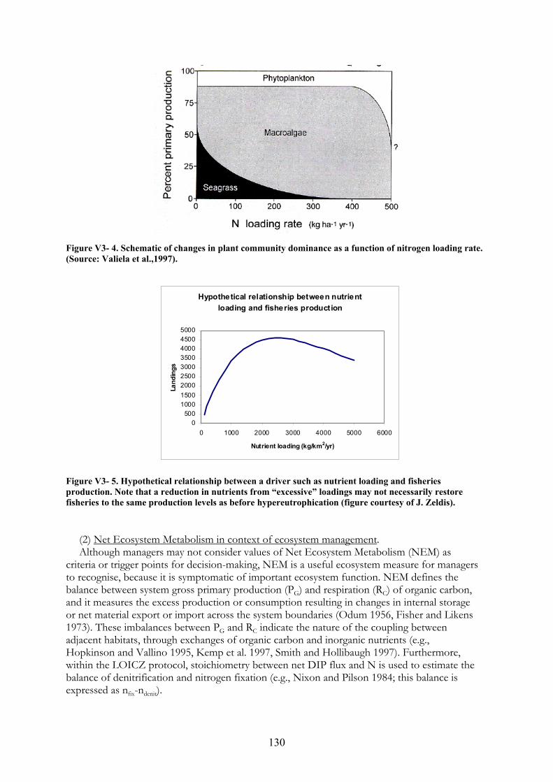
130

Hypothetical relationship between nutrient

loading and fisheries production

0

500

1000

1500

2000

2500

3000

3500

4000

4500

5000

0 1000 2000 3000 4000 5000 6000

Nutrient loading (kg/km2/yr)

Lan

din

gs

Figure V3- 4. Schematic of changes in plant community dominance as a function of nitrogen loading rate. (Source: Valiela et al.,1997). Figure V3- 5. Hypothetical relationship between a driver such as nutrient loading and fisheries production. Note that a reduction in nutrients from “excessive” loadings may not necessarily restore fisheries to the same production levels as before hypereutrophication (figure courtesy of J. Zeldis).

(2) Net Ecosystem Metabolism in context of ecosystem management. Although managers may not consider values of Net Ecosystem Metabolism (NEM) as

criteria or trigger points for decision-making, NEM is a useful ecosystem measure for managers to recognise, because it is symptomatic of important ecosystem function. NEM defines the balance between system gross primary production (PG) and respiration (RC) of organic carbon, and it measures the excess production or consumption resulting in changes in internal storage or net material export or import across the system boundaries (Odum 1956, Fisher and Likens 1973). These imbalances between PG and RC indicate the nature of the coupling between adjacent habitats, through exchanges of organic carbon and inorganic nutrients (e.g., Hopkinson and Vallino 1995, Kemp et al. 1997, Smith and Hollibaugh 1997). Furthermore, within the LOICZ protocol, stoichiometry between net DIP flux and N is used to estimate the balance of denitrification and nitrogen fixation (e.g., Nixon and Pilson 1984; this balance is expressed as nfix-ndenit).

131

NEP vs. DIN:TOC Loading Ratio

-100

0

100

200

0 1 2 3 4 5DIN:TOC Loading Ratio (gN gC-1)

Net

Ec

os

yst

em

Pro

du

ctio

n (

g C

m-2

y-1

)

Patuxent River

-40

-20

0

20

40

0.0 0.1 0.2 0.3

MERL

Ches. Bay

Narr. Bay

Patuxent R.

San Fran. Bay

Tomales Bay

Comparative analyses of NEM and nfix-ndenit suggest broad regional relationships with hydrology, watershed development and loading (Smith et al. 2003), which makes their use relevant for managers. In the Patuxent River estuary, USA (Kemp et al. 1999, Testa and Kemp 2008), the tight coupling between NEM and N cycling can be seen in the highly correlated patterns of annual mean rates of net O2 and DIN flux in both along the estuary axis and in hydrologically contrasting years (Figure I-3). In surface layers, DIN uptake generally corresponds to net O2 production (autotrophy), while in bottom layers net O2 consumption corresponds to net DIN production (heterotrophy). In years of higher DIN load, higher chlorophyll and O2 production indicates increased net-autotrophy (Figure I-3).

Whereas annual rates of primary production tend to be regulated by inputs of total nitrogen

for many coastal ecosystems (e.g., Boynton et al. 1982, Nixon 1986), it appears that NEM (i.e., PG – RC) is controlled more by the balance between inputs of DIN and total organic nitrogen, TON (or carbon, TOC), where DIN inputs stimulate PG, and TON (or TOC) inputs support RC (Kemp et al. 1997). For example, comparison of NEM and loading rates for five estuaries and for mesocosms (MERL; Oviatt et al. 1986) at different nutrient treatments reveals a consistent relationship between NEM and the DIN:TOC loading ratio (Figure V3-6).

Figure V3- 6. Comparison of NEM and loading rates for five estuaries and for mesocosms (MERL; Oviatt et al. 1986) at different nutrient treatments reveals a consistent relationship between NEP and the DIN:TOC loading ratio.

While strong relationships were evident for NEM from controlled experimental systems and for long term average rates in specific estuaries, substantial year-to-year variations are often evident for specific estuarine ecosystems. Such variations in metabolic rates may be related to fluctuations in climatic conditions that regulate, for example, inputs of organic matter from adjacent coastal upwelling regions (e.g., Smith and Hollibaugh 1997, Camacho-Ibar et al. 2003), or river flow and associated nutrient loading and water residence time. Values for PG and RC computed from continuous diel O2 measurements for a range of shallow North American coastal ecosystems revealed that NEM was generally negative (i.e., net heterotrophic), was responsive to climatic variations, and was related to N inputs (Caffrey 2004). In summary, we conclude that total primary production and NEM are tightly coupled to inputs and cycling of N

132

in most coastal environments, and that these relationships vary with hydrologic and climatic conditions, and are thus symptomatic of system behaviours that are important for managers.

(3) Role of coastal systems in mediating climatically important gases: It is likely that nutrient and carbon loading rates to coastal systems are pivotal in defining

their role in mediating climatically important gas fluxes (CO2, nitrous oxide, methane: Kroeze & Seitzinger 1998). Because of the relationships between loading, NEM and net denitrification, it is likely that nutrient accounts (as outlined above) from mass-balance studies (e.g., LOICZ) can yield information on this critical climate change issue. One hypothesis could be that denitrification is rendered less efficient under anoxic conditions and therefore N2O evolution may increase. Another could be that intensive agrarian land-use and associated organic loading can cause high methane emissions – such as appears to be occurring in the Waikato catchment of the Firth of Thames (C. Law NIWA pers. comm.). Are gas fluxes related in a consistent way with high nutrient loading and negative NEM across coastal systems?

(4) Role of coastal systems in maintaining / preventing anoxia: The resilience of coastal systems to anoxia may bear relation to physiographic characteristics

such as loading or residence time, data which are routinely available from LOICZ and other mass-balance analyses. Streeter-Phelps forecasts of anoxia could be made in systems which have oxygen data and LOICZ analyses, to check for such relationships. It is likely that a reasonable number of such datasets exist, to the extent that they could be classified by estuary type. The LOICZ data set could also be examined in the context of tipping points: is it possible to identify nutrient loading thresholds beyond which systems have altered states (e.g., tipped from sea-grass dominated to plankton- or bacteria-dominated)? If so, then recommendations could be made about maintaining nutrient loads below such thresholds. Note that once thresholds have been exceeded, many systems show hysteresis effects (Duarte et al. 2009), and do not return to the original state.

Other relationships that can be mined from the LOICZ data sets include examining the relationship of net ecosystem metabolism (NEM) to various measures of N:C inputs (Figure V3-6). In turn, NEM could be explored as an index relevant to fisheries.

Note that if total P (at least DRP+DOP) loading can be assumed (via Redfield ratios) to estimate TOC loading, its values could be used in this relation using LOICZ budgets typology data.

• Enhancement of extant LOICZ data sets with biological responses. LOICZ could invite the authors of its budgets to re-visit them, and to contribute data (if available) on biotic responses. If more data have been collected in the intervening time period, another assessment could be made to capture some temporal dynamics. This could be particularly useful if 10 or more years have elapsed.

• Effects of dams on the mix of nutrients entering coastal zones, and potential impacts on fish production. Dams present a clear conflict of ecosystem services. On the one hand, they provide a range of services from water provisioning, to hydroelectric power generation, to aesthetics. On the other, they have a range of adverse impacts on rivers, estuaries, and coastal zones, as well as their fish communities and fisheries. Freeman et al. (2003) provide an excellent review of the effects of dams on migratory animals, and others (e.g., Vorosmarty et al. 1997, Humborg et al. 2000, Ittekot et al. 2000, Vorosmarty et al. 2003) have demonstrated impacts of dams on hydrology, sediment loads, and nutrient fluxes. Conceivably, LOICZ could examine data sets from systems with impounded rivers to determine how nutrient ratios and absolute loads are affected. Fragmentation of these systems could also be quantified and related to changes in habitat use by diadromous fishes.

133

• Linking LOICZ budgets with the EcoPath-with-EcoSim (EwE) family of fisheries mass balance models. In an attempt to move away from single-species fishery management and its problems, Daniel Pauly and colleagues (e.g., Pauly et al. 2000) developed a series of network models to quantify relationships among communities of fishes and their food sources. Similar to the LOICZ nutrient approach, these models compute mass balances among different fish species within an ecosystem; in some cases, the computations have been taken down to the level of primary producers and nutrients). In the context of a coastal assessment, an EwE model would represent a subsystem that should be internally and externally consistent with the bounds imposed by a LOICZ assessment (i.e., there should not be more N, P, or C mass in the EwE model than what comes in).

It may also be relevant to couch such relationships as this in terms of “ecosystem services

and dis-services,” again reflecting a duality of effects. Other examples can include the impacts of bivalves on water clarity (a service often highly prized by people, Limburg et al. 2010) while at the same time the bivalves translocate nutrients to the sediments, thereby sometimes favoring nuisance macroalgae (a dis-service that could be quantified).

Other ideas

An important development needed to transfer coastal zone management benefits to managers in less developed countries is to extend newly developed hydrometric, GIS and modelling tools (e.g, REC, Sparrow, GlobalNews, Renuma) to those countries (e.g., India, South Pacific SE Asia, Africa). LOICZ should recommend that appropriate funding agencies (UNEP / UNDP / WOTRO / Embassies / Foreign Ministries) provide funding that would allow countries with these capacities to transfer hydrometric measurement and runoff/efflux modelling capacity to countries and regions where these capabilities do not exist or are poorly developed. We feel that relatively simple nutrient yield models or accounting methods are especially valuable in these applications. As datasets for developing countries mature, more sophisticated modelling approaches may become more appropriate. In other words, the complexity of the tools being applied in various regions must match the complexity of the data available to drive them.

134

Acknowledgements DPS and GG thank the other participants of the LOICZ budget methodology workshop for their enthusiasm, good ideas, and generosity with their time. We thank LOICZ for financial support for this workshop. Some of the time spent in organizing and conducting this workshop was supported by NOAA award NA05NOS478120, "Watershed-Estuary-Species Nutrient Susceptibility", NOAA Center for Sponsored Coastal Ocean Research, Coastal Hypoxia Research Program. Development and editing of the material in the written report was supported in part by the Baltic Nest Institute of the Stockholm Resilience Center, Stockholm University.

References Alhadeff, S.J., B.E. McCallum, and M.N. Landers. 2003. Water Resources Data - Georgia, 2003. United States Geological Survey, Compact Disk. Artioli, Y., Friedrich, J., Gilbert, A. J., McQuatters-Gollop, A., Mee, L. D., Vermaat, J. E., Wulff, F., Humborg, C., Palmeri, L., and Pollehne, F. 2008. Nutrient budgets for European seas: A measure of the effectiveness of nutrient reduction policies. Marine Pollution Bulletin. 56: 1609-1617. Atkinson, M.J. and Smith, S.V. 1983. C:N:P ratios of benthic marine plants. Limnology and Oceanography 28: 568-574. Auckland Regional Council. 2009. Aquaculture. http://www.arc.govt.nz/environment/coastal-and-marine/aquaculture/aquaculture_home. cfm (Webpage accessed January, 2010) Blomquist, S., A. Gunnars, and R. Elmgren. 2004. Why the limiting nutrient differs between temperate coastal seas and freshwater lakes: A matter of salt. Limnology and Oceanography. 49(6): 2236–2241 Boyer, E. W., C. L. Goodale, N. A. Jaworsk, and R. W. Howarth. 2002. Anthropogenic nitrogen sources and relationships to riverine nitrogen export in the northeastern USA. Biogeochemistry 57:137-169. Boynton W.R., Kemp W.M., Keefe C.W. 1982. A comparative analysis of nutrients and other factors influencing estuarine phytoplankton production. In: Kennedy VS (ed) Estuarine comparisons. Academic Press Ltd, New York, p 69-90. Boynton, W. R., J.H. Garber, R. Summers, and W.M. Kemp. 1995. Inputs, transformations, and transport of nitrogen and phosphorus in Chesapeake Bay and selected tributaries. Estuaries 18: 285-314. Boynton, W.R. and W.M. Kemp. 2008. Estuaries, pp. 809-856. In: Capone, D.G., Bronk, D.A., Mulholland, M.R. and Carpenter, E.J. (Eds.), Nitrogen in the Marine Environment 2nd Edition. Elsevier, Inc. Burlington, Massachusetts.

135

Breitburg, D. L., D.W. Hondorp, L.A. Davias & R.J. Diaz. 2009a. Hypoxia, nitrogen, and fisheries: integrating effects across local and global landscapes. Annual Review of Marine Science. 1: 329–349. Breitburg, D.L., L.A. Davias, K.E. Limburg, and D. P. Swaney. 2009b. Linking Nutrients, Hypoxia, Fisheries, and Fishes: Interim Report from a Workshop supported by LOICZ. LOICZ Inprint 2009/2:13-14. Bricker, S., B. Longstaff, W. Dennison, A. Jones, K. Boicourt, C. Wicks, and J. Woerner. 2007. Effects of Nutrient Enrichment In the Nation’s Estuaries: A Decade of Change. NOAA Coastal Ocean Program Decision Analysis Series No. 26. National Centers for Coastal Ocean Science, Silver Spring, MD. 328 pp. Broekhuizen, N., Zeldis. J. 2006. Forecasts of possible phytoplankton responses to elevated riverine nitrogen delivery into the southern Firth of Thames. NIWA Client Report: HAM2005-131.November 2005. (Client: Environment Waikato). http://www.ew.govt.nz/publications/technicalreports/tr0611.htm Burkart, M. R., and D. E. James. 1999. Agricultural-nitrogen contributions to hypoxia in the Gulf of Mexico. Journal of Environmental Quality 28:850-859. Caddy, J.F. 1993. Toward a comparative evaluation of human impacts on fishery ecosystems of enclosed and semi-enclosed seas. Reviews in Fisheries Science 1: 57–95. Caddy, J.F. 2000. Marine catchment basin effects versus impacts of fisheries on semi-enclosed seas. ICES Journal of Marine Science 57: 628-640. Caffrey, J. M. 2004. Factors controlling net ecosystem metabolism in U.S. estuaries. Estuaries 27: 90-101. Camacho-Ibar, V.F., Carriquiry, J.D., Smith, S.V. 2003. Non-conservative P and N fluxes and net ecosystem production in San Quintin Bay, México. Estuaries Vol 26(5): 1220-1237. Cederwall H., and R. Elmgren. 1980. Biomass increase of benthic macrofauna demonstrates eutrophication of the Baltic Sea. Ophelia Supplementum 1: 287-304. Close, M.E., Davies-Colley, R.J. 1990. Baseflow water chemistry in New Zealand rivers 1. Characterisation. New Zealand Journal of Marine and Freshwater Research 24:319-341. Common, M., and S. Stagl. 2005. Ecological Economics: an Introduction. Cambridge University Press, Cambridge, UK. Costanza, R., R. d'Arge, R. de Groot, S. Farber, M. Grasso, B. Hannon, K. Limburg, S. Naeem, R.V. O'Neill, J. Paruelo, R.G. Raskin, P. Sutton, and M. van den Belt. 1997. The value of the world's ecosystem services and natural capital. Nature 387: 253-260. Costanza, R., J. Cumberland, H. Daly, R. Goodland, and R. Norgaard. 1997. An Introduction to Ecological Economics. CRC Press, Boca Raton, FL. Costanza, R., S. O. Funtowicz, and J. R. Ravetz. 1992. Assessing and communicating data quality in policy-relevant research. Environmental Management 16:121–131.

136

Crossland, C.J.; Kremer, H.H.; Lindeboom, H.J.; Marshall Crossland, J.I.; Le Tissier, M.D.A. (eds). 2005a. Coastal Fluxes in the Anthropocene. The Land-Ocean Interactions in the Coastal Zone Project of the International Geosphere-Biosphere Programme. Springer-Verlag, Berlin Heidelberg. Crossland, C.J., D. Baird, J.-P. Ducrotoy, and H. Lindeboom. 2005b. The Coastal Zone – a Domain of Global Interactions. Chapter 1 in: Crossland, C.J.; Kremer, H.H.; Lindeboom, H.J.; Marshall Crossland, J.I.; Le Tissier, M.D.A. (eds). Coastal Fluxes in the Anthropocene. The Land-Ocean Interactions in the Coastal Zone Project of the International Geosphere-Biosphere Programme. Springer-Verlag, Berlin Heidelberg. Daily, G. (ed.) Nature’s Services: Societal Dependence on Natural Ecosystems. Island Press, Washington, DC. Daily, G.C., S. Alexander, P.R. Ehrlich, L. Goulder, J. Lubchenco, P.A. Matson, H.A. Mooney, S. Postel, S.H. Schneider, D. Tilman, and G.M. Woodwell. 1997. Ecosystem Services: Benefits Supplied to Human Societies by Natural Ecosystems. Issues in Ecology 2. Ecological Society of America, Washington, D.C. David, M. B., and L. E. Gentry. 2000. Anthropogenic inputs of nitrogen and phosphorus and riverine export for Illinois, USA. Journal of Environmental Quality 29:494-508. Dentener, F. J., and P. J. Crutzen. 1994. A 3-Dimensional Model of the Global Ammonia Cycle. 19:331-369. Downing, J.A., C. Plante, and S. Lalonde. 1990. Fish production is correlated with primary productivity, not the morphoedaphic index. Canadian Journal of Fisheries and Aquatic Sciences 47: 1929-1036. Duarte, C.M. 1995. Submerged aquatic vegetation in relation to different nutrient regimes. Ophelia 41: 87-112. Duarte, C.M., D.J. Conley, J. Carstensen, and M. Sanchez-Camacho. 2009. Return to Neverland: shifting baselines affect eutrophication restoration targets. Estuaries and Coasts 32: 29-36. (EDC) Earth Resources Observation Systems (EROS) Data Center 2000. Global Land Cover Characterization. EROS Data Center Distributed Active Archive Center. http://edcdaac.usgs.gov/ . Ellis, E. C., R. G. Li, L. Z. Yang, X. Cheng. 2000. Long-Term Change In Village-Scale Ecosystems In China Using Landscape And Statistical Methods. Ecological Applications 10:1057-1073 Farley, J., J.D. Erickson, H.E. Daly. Ecological Economics: a Workbook for Problem-Based Learning. Island Press, Washington, D.C. Fisher, S. G., and G.E. Likens. 1973. Energy Flow in Bear Brook, New Hampshire - Integrative Approach to Stream Ecosystem Metabolism. Ecological Monographs 43: 421-439.

137

Food and Agriculture Organization of the United Nations (FAO) 2001. FAOSTAT: FAO Statistical Databases. Accessible through the Food and Agriculture Organization of the United Nations. http://faostat.fao.org/. Fox, L. E., S. L. Sager, and S. C. Wofsy. 1985. Factors controlling the concentrations of soluble phosphorus in the Mississippi estuary. Limnol. Oceanogr. 30: 826-832. Fox, L.E. 1989. A model for inorganic control of phosphate concentrations in river waters. Geochim Cosmochim Acta 53: 417–418. Freeman, M.C., C.M. Pringle, E.A. Greathouse, and B.J. Freeman. 2003. Ecosystem-level consequences of migratory faunal depletion caused by dams, pp. 255-266 In K.E. Limburg and J.R. Waldman, editors. Biodiversity,Status, and Conservation of Shads Worldwide. American Fisheries Society Symposium 35. Froelich, P.N. N. A. Luedtke, G. R. Heath, and T. DeVries. 1982. The marine phosphorus cycle. Am. J. Sci. 282: 475-511. Froelich, P.N. 1988. Kinetic control of dissolved phosphate in natural rivers and estuaries: A primer on the phosphate buffer mechanism. Limnology and Oceanography. 33(4, part 2):649-668. Galloway, J. N., J. D. Aber, J. W. Erisman, S. P. Seitzinger, R. W. Howarth, E. B. Cowling, and B. J. Cosby. 2003. The nitrogen cascade. Bioscience 53:341-356. Gazeau, F., A. V. Borges, C. Barrón, C. M. Duarte, N. Iversen, J. J. Middelburg, B. Delille, M.-D. Pizay,M. Frankignoulle, J.-P. Gattuso. 2005. Net ecosystem metabolism in a micro-tidal estuary (Randers Fjord, Denmark): evaluation of methods. Marine Ecology Progress Series 301: 23–41 Giordani, G., Austoni, M., Zaldívar, J.M., Swaney, D.P. and P. Viaroli. 2008. Modelling ecosystem functions and properties at different time and spatial scales in shallow coastal lagoons: an application of the LOICZ biogeochemical model. Estuarine, Coastal and Shelf Science 77/2: 264-277. DOI information: 10.1016/j.ecss.2007.09.017 Giordani, G. P. Viaroli, D.P. Swaney, C.N. Murray, J.M. Zaldívar and J.I. Marshall Crossland. 2005. Nutrient fluxes in transitional zones of the Italian coast. LOICZ Reports and Studies Series, Volume 28. http://www.loicz.org/imperia/md/content/loicz/print/rsreports/report28small.pdf Gonzalez-De Zayas, R. Unpublished Ph.d. dissertation. Universidad Nacional Autónoma de México. México, D.F. 04510. Goolsby, D. A., W. A. Battaglin, B. T. Aulenbach, and R. P. Hooper. 2000. Nitrogen flux and sources in the Mississippi River Basin. Science of the Total Environment 248:75-86. Goolsby, D. A., W. A. Battaglin, B. T. Aulenbach, and R. P. Hooper. 2001. Nitrogen input to the Gulf of Mexico. Journal of Environmental Quality 30:329-336. Gordon, D. C., Jr., P. R. Boudreau, K. H. Mann, J.-E. Ong, W. L. Silvert, S. V. Smith, G. Wattayakorn, F. Wulff, and T. Yanagi. 1996. LOICZ Biogeochemical Modelling Guidelines.

138

Land-Ocean Interactions in the Coastal Zone, LOICZ Reports & Studies 5. Texel, The Netherlands. Gowdy, J.M. 1997. The value of biodiversity: markets, society, and ecosystems. Land Economics 73: 25-41. Green, P. A., C. J. Vorosmarty, M. Meybeck, J. N. Galloway, B. J. Peterson, and E. W. Boyer. 2004. Pre-industrial and contemporary fluxes of nitrogen through rivers: a global assessment based on typology. Biogeochemistry 68:71-105. Gupta, G. V. M., U. Natesan, M. V. Ramana Murthy, V. G. Sravan Kumar, S. Viswanathan, M. S. Bhat, A. K. Ray, and B. R. Subramanian. 2006. Nutrient budgets for Muthupet lagoon, southeastern India. Current Science, 90:967-972. Han, H. 2007. Nutrient loading to Lake Michigan: A mass balance assessment. University of Michigan Ann Arbor. Harmon, T.C., S. Villamizar Amaya, C. A. Butler, H. Pai, P. Barnes, J. Fisher, F. Silva, T. Stathopoulos, and W. Kaiser. 2009. Closing the Loop on Groundwater-Surface Water Interactions, River Hydrodynamics, and Metabolism on the San Joaquin River Basin. UCLA: Center for Embedded Network Sensing. Retrieved from: http://escholarship.org/uc/item/40d148r2 , February 2, 2012. Hauraki Gulf Forum 2004. The Hauraki Gulf State of the Environment Report. 223 pp. http://www.arc.govt.nz/arc/fms/coast/soe05a.pdf Helfman, G.S. 2007. Fish Conservation: A Guide to Understanding and Restoring Global Aquatic Biodiversity and Fisheries Resources. Island Press, Washington, D.C. Hondorp, D.W., D.L. Breitburg, and L. Davias. 2007. Impacts of eutrophication and hypoxia on the composition of fisheries landings. Estuarine Research Federation biennial conference (abstract). Hopkinson C.S., Vallino J.J. 1995. The relationships among man’s activities in watersheds and estuaries: a model of runoff effects on patterns of estuarine community metabolism. Estuaries 18: 598-621. Howarth R.W., Marino R., Garritt R., Sherman D. 1992. Ecosystem respiration and organic carbon processing in a large, tidally influenced river: the Hudson River. Biogeochemistry 16: 83-102. Howarth, R. W., H. Jensen, R. Marino & H. Postma. 1995. Transport to and processing of phosphorus in near-shore and oceanic waters. Pages 323-345. In: H. Tiessen (ed.), Phosphorus in the Global Environment, SCOPE #54. Wiley & Sons, Chichester. Howarth, R. W., G. Billen, D. Swaney, A. Townsend, N. Jaworski, K. Lajtha, J. A. Downing, R. Elmgren, N. Caraco, T. Jordan, F. Berendse, J. Freney, V. Kudeyarov, P. Murdoch, and Z. L. Zhu. 1996. Regional nitrogen budgets and riverine N&P fluxes for the drainages to the North Atlantic Ocean: natural and human influences. Biogeochemistry 35:75-139.

139

Howarth, R. W., E. W. Boyer, W. J. Pabich, and J. N. Galloway. 2002. Nitrogen use in the United States from 1961-2000 and potential future trends. Ambio 31:88-96. Howarth, R. W., D. P. Swaney, E. W. Boyer, R. Marino, N. Jaworski, and C. Goodale. 2006. The influence of climate on average nitrogen export from large watersheds in the Northeastern United States. Biogeochemistry 79:163-186. Humborg, C., D.J. Conley, L. Rahm, F. Wulff, A. Cociasu, and V. Ittekkot. 2000. Silicon retention in river basins: far-reaching effects on biogeochemistry and aquatic food webs in coastal marine environments. Ambio 29: 45-50. Ittekkot, V., C. Humborg, and P. Schäfer. 2000. Hydrological alterations and marine biogeochemistry: a silicate issue? BioScience 50: 776-782. Jordan, T. E., and D. E. Weller. 1996. Human contributions to terrestrial nitrogen flux. Bioscience 46:655-664. Kemp W.M., Smith E.M., Marvin-DiPasquale M., Boynton W.R. 1997. Organic carbon balance and net ecosystem metabolism in Chesapeake Bay. Mar Ecol Prog Ser 150: 229-248. Kemp W.M., Puskaric S., Faganeli J., Smith E.M., Boynton W.R. 1999. Pelagic-benthic coupling and nutrient cycling. In: Malone TC, Malej A, Harding LW Jr, Smodlaka N, Turner RE (eds) Coastal and estuarine studies, ecosystems at the land-sea margin: drainage basin to coastal sea. American Geophysical Union, Washington, DC, p 295-339. Kroeze C. and Seitzinger S.P. 1998. The impact of land use on N2O emissions from watersheds draining into the Northeastern Atlantic Ocean and European Seas. Environ. Pollut. 102(Suppl.): 149–158. Lehrter, J.C. and J. Cebrian. 2010. Uncertainty propagation in an ecosystem nutrient budget. Ecological Applications. 20:508-524. Le Tissier, M.D.A, R. Buddemeier, J. Parslow, D.P. Swaney, C.J. Crossland, S.V. Smith, H.A.Y Whyte, W.C. Dennison, J.M. Hills, and H. Kremer. 2006. The role of the coastal ocean in the disturbed and undisturbed nutrient and carbon cycles – A management perspective. LOICZ, Geesthacht, Germany. Limburg, K.E., V. Luzadis, M.M. Ramsey, K.L. Schulz, and C.M. Mayer. 2010. The good, the bad, and the algae: ecosystem services and disservices generated by zebra and quagga mussels. Journal of Great Lakes Research 36: 86-92. Liu, S. M., G.-H. Hong, X. W. Ye, J. Zhang, and X. L. Jiang. 2009. Nutrient budgets for large Chinese estuaries and embayment. Biogeosciences Discussions. 6, 391–435. Liu, Y. and D. Scavia. 2010. Analysis of the Chesapeake Bay Hypoxia Regime Shift: Insights from Two Simple Mechanistic Models. Estuaries and Coasts 33:629–639. McGlathery, K. J., R. W. Howarth, and R. Marino. 1992. Nutrient Limitation of the Macroalga, Penicillus-Capitatus, Associated with Subtropical Seagrass Meadows in Bermuda. Estuaries 15:18-25.

140

McGlathery, K. J., R. Marino, and R. W. Howarth. 1994. Variable Rates of Phosphate-Uptake by Shallow Marine Carbonate Sediments - Mechanisms and Ecological Significance. Biogeochemistry 25:127-146. Millennium Ecosystem Assessment. 2005. Ecosystems and Human Well-being: Synthesis. Island Press, Washington, DC. Miller, R.L. and B.F. McPherson .1991. Estimating estuarine flushing and residence times in Charlotte Harbor, Florida, via salt balance and a box model. Limnology and Oceanography 36: 602-612. Morgan, M. G., and M. Henrion .1990. Uncertainty: A guide to dealing with uncertainty in quantitative risk and policy analysis. Cambridge University Press, New York. Nixon, S. W. and M. E. Q. Pilson. 1984. Estuarine total system metabolism and organic exchange calculated from nutrient ratios: An example from Naragansett Bay, p. 261-290. In V. S. Kennedy [ed.], The Estuary as a Filter. Academic Press, Inc. Nixon, S.W. 1986. Nutrient dynamics and the productivity of marine coastal waters, p. 97-115. In R. Halwagy et al. (eds.), Marine environment and pollution. Alden. Nixon, S.W. 1988. Physical Energy Inputs and the Comparative Ecology of Lake and Marine Ecosystems. Limnology and Oceanography 33: 1005-1025. Odum, H. T. 1956. Primary Production in Flowing Waters. Limnology and Oceanography 1: 102-117. Odum, E.P., J.T. Finn, and E.H. Franz .1979. Perturbation theory and the subsidy-stress gradient. BioScience 29: 349-352. Officer, C. B. .1980.: Box models revisited. In P. Hamilton and K. B. Macdonald (eds.): Estuarine and Wetland Processes with Emphasis on Modeling, pp. 65–114. Plenum Press, New York. Oglesby, R.T. .1977. Relationships of fish yield to lake phytoplankton standing crop, production and morphoedaphic factors. Journal of the Fisheries Research Board of Canada 34: 2271-2279. Oviatt, C. A., A.A. Keller, P.A. Sampou, and L.L. Beatty .1986. Patterns of productivity during eutrophication: a eutrophication experiment Marine Ecology Progress Series 28: 69-80. Pauly, D., V. Christensen, and C. Walters . 2000. Ecopath, Ecosim, and Ecospace as tools for evaluating ecosystem impacts of fisheries. ICES Journal of Marine Science 57: 697-706. Pritchard, D.W. 1969. Dispersion and flushing of pollutants from estuaries. Proceedings of the American Society of Civil Engineers 95, HY1: 115-124. Rabalais, N. N., R. J. Díaz, L. A. Levin, R. E. Turner, D. Gilbert, and J. Zhang. 2009. Dynamics and distribution of natural and human-caused coastal hypoxia, Biogeosciences Discuss. 6: 9359-9453. Rysgaard, S., P. Thastum, T. Dalsgaard, P.B. Christensen, and N.P. Sloth. 1999. Effects of salinity on NH4+ adsorption capacity, nitrification, and denitrification in Danish estuarine sediments. Estuaries 22: 21-30.

141

Scavia, D. and K.A. Donnelly. 2007. Reassesing Hypoxia Forecasts for the Gulf of Mexico. Env. Sci. Technol. 41: 8111–8117. Schiettecatte, L.S., F. Gazeau, Van der Zee, C., Brion, N., Borges, A. 2006. Time series of the partial pressure of carbon dioxide (2001 2004) and preliminary inorganic carbon budget in the Scheldt plume (Belgian coast waters). Geochemistry, Geophysics, Geosystems (G3). 7: 1-16. doi:10.1029/2005GC001161 Seitzinger, S.P. 1988. Denitrification in freshwater and coastal marine ecosystems: ecological and geochemical significance. Limnology and Oceanography 33: 702-724. . Sheldon, J.E. and M. Alber. 2002. A comparison of residence time calculations using simple compartment models of the Altamaha River estuary, Georgia. Estuaries 25: 1304-1317. Sheldon, J.E. and M. Alber. 2005. Comparing transport times through salinity zones in the Ogeechee and Altamaha River estuaries using SqueezeBox. In K.J. Hatcher (ed.) Proceedings of the 2005 Georgia Water Resources Conference. Institute of Ecology, University of Georgia, Athens, GA. Sheldon, J.E., and M. Alber , 2006. The calculation of estuarine turnover times using freshwater fraction and tidal prism models: a critical evaluation, Estuaries Coasts 29: 133–146. Sheldon, J.E. and M. Alber. (unpubl.). Presentation: Beyond whole-estuary flushing times: Using transport times through salinity zones to explain chlorophyll patterns in the Altamaha River estuary (Georgia, USA). Estuarine Interactions: biological-physical feedbacks and adaptations. 2005 Estuarine Research Federation Meeting. October 16-20, 2005, Norfolk, VA. Smith, S.V.; Hollibaugh, J.T.; Dollar, S.J.; Vink, S. 1991. Tomales Bay metabolism: C-N-P stoichiometry and ecosystem heterotrophy at the land-sea interface. Estuarine, Coastal and Shelf Science 33: 223-257. Smith, S. V., and J. T. Hollibaugh .1997. Annual cycle and interannual variability of net and gross ecosystem metabolism in a temperate climate embayment. Ecological Monographs. 67:509-533. Smith, S.V., V. Dupra, J.I. Marshall Crossland and C.J. Crossland. 2000. Estuarine systems of the East Asia region: carbon, nitrogen and phosphorus fluxes. LOICZ Reports and Studies Series, Volume 16. http://www.loicz.org/imperia/md/content/loicz/print/rsreports/report16.pdf Smith S.V. 2002. Carbon-nitrogen-phosphorus fluxes in the coastal zone: the global approach. IGBP Global Change Newsletter 49: 7–11. Smith, S. V., D.P. Swaney, L. Talaue-Mcmanus, J.D. Bartley, P.T. Sandhei, C.J. Mclaughlin, V.C. Dupra, C.J. Crossland, R. W. Buddemwier, B.A. Maxwell, and F. Wulff. 2003. Humans, Hydrology, and the Distribution of Inorganic Nutrient Loading to the Ocean. Bioscience 53: 235-345. Smith, S. V., R. W. Buddemeier, F. Wulff, and D. P. Swaney. 2005. C, N, P Fluxes in the Coastal Zone. Chapter 3 in: Crossland, C.J.; Kremer, H.H.; Lindeboom, H.J.; Marshall Crossland, J.I.; Le Tissier, M.D.A. (eds). Coastal Fluxes in the Anthropocene. The Land-Ocean Interactions in the

142

Coastal Zone Project of the International Geosphere-Biosphere Programme. Springer-Verlag, Berlin Heidelberg.

Smith, S.V., D.P. Swaney, and L. Talaue-McManus. 2010. Carbon–Nitrogen–Phosphorus Fluxes in the Coastal Zone: The LOICZ Approach to Global Assessment. Chapter 14 (pp 575-586) in: Carbon and Nutrient Fluxes in Continental Margins A Global Synthesis Series: Global Change - The IGBP Series. Liu, K.-K.; Atkinson, L.; Quiñones, R.; Talaue-McManus, L. (Eds.) 2010, XXVIII, 744 pp. Soto-Galera, E., J. Paulo-Maya, E. Lopez-Lopez, J.A. Sana-Hernandez, and J. Lyons. 2004. Change in fish fauna as indication of aquatic ecosystem condition in Rio Grande de Morelia–Lago de Cuitzeo Basin, Mexico. Environmental Management 24: 133-140. Stow, C.A. and D. Scavia. 2009. Modeling Hypoxia in the Chesapeake Bay: Ensemble Estimation Using a Bayesian Hierarchical Model. J. Marine Systems 76: 244-250. Swaney, D.P. (2011): Biogeochemical budgeting in estuaries. In: Laane, R.W.P. and J.J. Middelburg (eds.): Treatise on Estuarine and Coastal Science 5: 343-362. Swaney, D.P., S.V. Smith, and F. Wulff. 2011. The LOICZ Biogeochemical modeling protocol and its application to estuarine ecosystems. In: Baird, D and A. Mehta (eds.), Treatise on Estuarine and Coastal Science 9: 135-159. Talaue-McManus, L., S.V. Smith and R.W. Buddemeier. 2003. Biophysical and socio-economic assessments of the coastal zone: the LOICZ approach. Ocean & Coastal Management 46: 323–333 Testa, J.M. and W.M. Kemp. 2008. Variability of biogeochemical processes and physical transport in a partially stratified estuary: A box-modeling analysis. Marine Ecology Progress Series 356:63–79 Testa, J.M., Kemp, W.M., Boynton, W.R., and Hagy, J.D. 2008. Long-Term Changes in Water Quality and Productivity in the Patuxent River Estuary: 1985 to 2003. Estuaries and Coasts 31: 1021–1037

Thomas, H., Bozec, Y., Elkalay, K., and de Baar, H.J.W. 2004. Enhanced Ocean Storage of CO2 From Shelf Sea Pumping. Science 304: 1005-1008. Valiela, I., J. McClelland, J. Hauxwell, P.J. Behr, D. Hersh, and K. Foreman. 1997. Macroalgal blooms in shallow estuaries: controls and ecophysiological and ecosystem consequences. Limnology and Oceanography 42: 1105–1118.

Van Breemen, N., E. W. Boyer, C. L. Goodale, N. A. Jaworski, K. Paustian, S. P. Seitzinger, K. Lajtha, B. Mayer, D. Van Dam, R. W. Howarth, K. J. Nadelhoffer, M. Eve, and G. Billen. 2002. Where did all the nitrogen go? Fate of nitrogen inputs to large watersheds in the northeastern USA. Biogeochemistry 57: 267-293. Van Drecht, G., A. F. Bouwman, E. W. Boyer, P. Green, and S. Siebert. 2005. A comparison of global spatial distributions of nitrogen inputs for nonpoint sources and effects on river nitrogen export. Global Biogeochemical Cycles 19.

143

Viaroli, P., G. Giordani, M. Bartoli, M. Naldi, R. Azzoni, D. Nizzoli, I. Ferrari, J.M. Zaldìvar Comenges, S. Bencivelli, G. Castaldelli and E.A. Fano. 2006. The Sacca di Goro Lagoon and an Arm of the Po River. In Peter J. Wangersky (eds.): The Handbook of Environmental Chemistry. Springer-Verlag GmbH. Volume H / 2006. Title: Estuaries. pp. 197 – 232. DOI: 10.1007/698_5_030. Vörösmarty, C.J., K. Sharma, B. Fekete, A.H. Copeland, J. Holden, J. Marble, and J.A.Lough. 1997. The storage and aging of continental runoff in large reservoir systems of the world. Ambio 26: 210– 219. Vörösmarty, C.J. and Peterson B.J. 2000. Macro-scale models of water and nutrient flux to the coastal zone. In: Hobbie J.E. (ed) Estuarine Science: A Synthetic Approach to Research and Practice. Island Press, Washington, DC. Vörösmarty, C. J., M. Meybeck, B.M. Fekete, K. Sharma, P. Green, and J. Syvitski. 2003. Anthropogenic sediment retention: Major global-scale impact from the population of registered impoundments, Global and Planetary Change 39: 169-190. Webster, I.T., J. S. Parslow, and S. V. Smith. 2000. Implications of spatial and temporal variation for biogeochemical budgets of estuaries. Estuaries 23: 341-350. Wilkie, J. 1914. From Tasman To Marsden: A History of Northern New Zealand from 1642 to 1818. Robert McNab. Dunedin New Zealand Electronic Text Centre. http://www.nzetc.org/tm/scholarly/name-101193.html . Winker, C.D., L.C. Jaffe, and J.D. Howard. 1985. Georgia estuarine data 1961-1977. Georgia Marine Science Center, University System of Georgia, Technical Report Series 85-7. Skidaway Island, GA. Wulff, F., O. P. Savchuk, A. Sokolov, C. Humborg & C. M. Mörth. 2007. Management options and effects on a marine ecosystem: Assessing the future of the Baltic. Ambio 36: 243-249. Yanagi, T. 2000. Simple method for estimating Vx from mixing equations in a 1-dimensional, steady-state system for LOICZ biogeochemical modelling. Pages 108-110 in Dupra, V., Smith, S.V., Marshall Crossland, J.I. and Crossland, C.J. 2000. Estuarine systems of the East Asia region: carbon, nitrogen and phosphorus fluxes. LOICZ Reports and Studies 16, LOICZ, Texel, The Netherlands, 127 pp. Zaldivar, J.M., E. Cattaneo, M. Plus, C.N. Murray, G. Giordani, P. Viaroli. 2003. Long-term simulation of main biogeochemical events in a coastal lagoog: Sacca di Goro (Northern Adriatic Coast, Italy). Continental Shelf Research 23: 1847-1875. Zeebe, R. E. and D. A. Wol-Gladrow. 2001. CO2 in seawater, equilibrium, kinetics, isotopes. Amsterdam Elsevier Oceanography Series 65: 346. Zeldis, J.R. 2004. New and remineralised nutrient supply and ecosystem metabolism on the northeastern New Zealand continental shelf. Continental Shelf Research 24: 563-581. Zeldis, J. 2005. Magnitudes of natural and mussel farm-derived fluxes of carbon and nitrogen in the Firth of Thames. Prepared by John Zeldis (NIWA) for Environment Waikato. NIWA Client

144

Report CHC2005-048, NIWA Project EWR05504. Environment Waikato Technical Report 2005/30. www.ew.govt.nz/PageFiles/10964/TR0816.pdf Zeldis, J. 2006. Water, Salt and Nutrient Budgets for Hauraki Gulf and adjacent Firth of Thames, New Zealand. LOICZ website: http://nest.su.se/mnode/new_zealand/HaurakiGulf/Hauraki_revised/Hauraki%20budget%2004revised.htm Zeldis, J. 2007. ‘Origin and processing of nutrients in Golden and Tasman Bays’. Tasman District Council Envirolink Advice Grant (October 2007). Zeldis, J. 2008a. Origin and processing of nutrients in Golden and Tasman Bays. Tasman District Council. NIWA Client Report : CHC2008-052. www.tdc.govt.nz/pdfs/chc2008_052.pdf Zeldis, J. 2008b. Exploring the Carrying Capacity of the Firth of Thames for Finfish Farming: A Nutrient Mass-Balance Approach. Report: TR 2008/16, Waikato Environment, Hamilton, NZ. http://www.ew.govt.nz/Publications/Technical-Reports/TR200816/

145

Appendix I. Aquatic Ecosystem Services

(from: Encyclopedia of Inland Waters (G.E.Likens, editor; Elsevier 2008)

Karin E. Limburg State University of New York, College of Environmental Science and Forestry

Syracuse, NY 13210 USA Phone: 1-315-470-6741; Fax: 1-315-470-6934

Email: [email protected] Synopsis: Aquatic ecosystem goods and services are the stocks and flows deriving from ecosystem processes that have some value to humankind. These values may be direct and apparent, such as the economic value of fisheries; or they may be generated from indirect or unapparent means, such as the benefits accrued from groundwater processes that purify drinking water. A number of methods are used to quantify aquatic and other ecosystem services, but this science is still in its infancy, and many issues are not resolved. Among the threats to ecosystem services are the familiar problems of habitat loss and fragmentation, pollution, and over-use, all of these exacerbated by the increasing populations of humans as well as their increasing patterns of consumption. Ecosystem service valuation is one way to make the “hidden subsidies of Nature” visible and quantifiable. Key words: Ecosystem service, value, valuation

Introduction

What’s a sunset on a still lake worth? Or a sip from a spring on a summer bike ride? What inspires novels, poems, and essays about water? These questions raise the idea of value, in terms that might relate directly to many people’s experience. Other kinds of value are not as readily perceived. For example, there is value in a clean river, or in ground water that is available for plant uptake and evapotranspiration. There is value in the cooling and heating properties of lakes, rivers, and the ocean. And there is value in the existence of healthy fish communities that may provide both protein and recreational pleasure. Collectively, ecologists and others have begun to refer to these different kinds of values as ecosystem services. The concept gained attention during the 1990s as scientists began to realize that natural ecosystems were being damaged and destroyed by humans at unprecedented rates, due to human population growth and the resulting increased exploitation of natural resources. Further, there was concern that this environmental damage might not only be irreparable in many cases, but might also fundamentally alter global cycles, such as the hydrological cycle or the global climate. Scientists feared that many ecosystem properties would be altered or lost before understanding their importance, for example biodiversity in many systems. Ecologists coined the term “ecosystem services” as a way of conveying the idea that ecological systems provide services, in addition to goods, that underpin human well-being. These goods and services provide value to humanity in both direct and indirect ways. Notions of Value No one knows precisely how long humans have held formalized concepts of value, but the philosophical roots go back at least several thousand years. The Greek philosopher Aristotle struggled with the value of using things, versus the value of exchanging things, and how there could be parity between them. An often-cited example of the difference between use and

146

exchange value is the “diamonds and water paradox.” Water, which is essential for life, has been extremely cheap, historically; on the other hand, diamonds, which are exchangeable luxury items, are extremely expensive. The history of economic thought embodies the search for measures of value, wealth, and exchange. This chapter will not go into this history, but references are included in “Further Reading.” Essentially, value is the difference that something makes to someone; it may be tangible and apparent, like a durable good, or it may be something that people overlook in their day-to-day activities. The value of many ecosystem services falls into the latter category. It is also true that value is subjective and contextual. The value of some ecosystem services in a generally deteriorating environment may be higher than in a “pristine” world. Classification of Ecosystem Services and Natural Capital Ecosystem services are broken down into a number of categories. The Millennium Ecosystem Assessment listed four broad categories:

• Provisioning services are those that provide goods such as food and water; • Regulating services are those that control various processes, such as flood control or

suppression of disease outbreaks; • Supporting services, such as nutrient recycling, maintain material and energy balances;

and • Cultural services are those that provide spiritual, moral, and aesthetic benefits.

To this, we may add other types of services, such as provision of habitat, or information flow (science and education). A selection of examples of ecosystem services from aquatic systems are given in Table A-0. Some are obvious, such as the production of food and other exploitable products, or the provision of recreational opportunities. Some are less apparent, such as the storage and purification of water in aquifers, the ameliorating influence of large lakes on local climate, the role of the world’s oceans in regulating global climate, or the assimilation of wastes by biogeochemical processing. Another distinction that is often made is between “ecosystem services” and “natural capital.” Following economic terminology, capital is the standing stock of a good or information (represented by money); hence, natural capital is the standing stock of environmental goods. Natural capital generates flows of ecosystem services, either on their own or together with capital flows from other resources. An example of autonomous production of a service from natural capital might be the provisioning of protein from an animal community, such as oysters in an estuary. An example of natural capital flows combining from different systems might be the movement of detritus through a river ecosystem into a recipient estuary; the detritus is transformed on its journey and fuels different food webs, some of which may ultimately provide food or other services. The concept of ecosystem services is inherently biased toward the anthropocentric perspective. The reason is two-fold: first, a major point of discussing ecosystem services is to highlight their utility and essentiality for humans in an economic world which increasingly marginalizes the value of undeveloped, natural ecosystems; and second, although ecosystems do not “care” about whether Homo sapiens exists among all other species, we do, and thus we recognize that ecosystem goods and services are the natural components and processes that cannot be compromised, if our species is to persist. Moreover, ecosystem functionality depends on access to these goods and services by non-human organisms as well. In contrast to the

147

commonly held, layperson’s view that the natural world is a sub-system of the human world, the concept of ecosystem services helps us to see how human societies are, in fact, embedded within the natural world. Valuing Ecosystem Goods and Services Although the importance of ecosystem goods and services is recognized, quantifying these has been at times challenging and controversial. Some quantification has taken the form of economic valuation, using accepted methods. Where markets exist, valuation in monetary terms is fairly straightforward, even if it does not necessarily capture all the value. For example, fish markets capture the value of fish as food, but not their value in food webs per se. Methods used by environmental and ecological economists include:

• Avoided cost: the cost that an individual or society avoids paying because of the natural service. For example, fringing mangroves and other coastal wetlands can buffer coastlines from storm damage. In 2005, Hurricanes Katrina and Rita inflicted damage along the U.S. Gulf of Mexico coast that ran into the tens of billions of dollars; much of that could have been avoided, had wetlands been left intact.

• Replacement cost: the cost that individuals or society would have to pay if the natural service did not exist. An example is the use of cypress wetlands in the Southeastern U.S. to “polish” treated wastewater, stripping out nutrients that otherwise would have to be treated with expensive tertiary wastewater treatment.

• Travel cost: some ecosystem goods and services require travel to appreciate, implying the costs willingly borne by people to “utilize” the good or service. This approach is a common method to assess the minimum value of parks, recreational areas and activities.

• Factor Income: the degree to which a service enhances incomes. For example, improvements in water quality may enhance the tourism sector.

• Hedonic Pricing: a de facto analysis of goods associated with ecosystem services. Real estate prices near a lake or a beach typically are much greater than a few miles inland, reflecting the appeal of the water or shoreline to humans.

• Contingent Valuation: a survey-based method to evaluate individuals’ willingness to pay for increased flow of a service, or willingness to accept the costs of maintaining a service, through the posing of hypothetical scenarios. An example would be the willingness not to develop near a sensitive wetland area.

• Option and Insurance Values: although these may be more difficult to compute, these are values of ecosystem services that provide options in the face of uncertainty. An example is the potential for new uses to be found through “prospecting” for pharmaceuticals in corals, or maintenance of intact riparian zones along a floodplain (rather than building thereon). A variant on option value is “bequest value,” that is, the value that is to be left to future generations. A landmark study of the total value of Earth’s ecosystem goods and services (see Further

Reading), conducted as a valuation exercise in the mid-1990s, arrived at an estimated worth of $33.3 trillion dollars, nearly double the global Gross Domestic Product (GDP). Controversy ensued, as economists faulted the methods used, and ecologists argued that monetary valuation did not truly capture ecosystem value. Nevertheless, this and other case studies have brought to light that ecosystems, even disturbed ones, provide value to society.

148

Examples of Ecosystem Services Generation in Aquatic Ecosystems Wetlands Wetlands have received a great deal of study over the past 40 years, and have become recognized as ecosystems with many valuable properties. As a result, many wetlands are now protected the world over, or if they are destroyed, replacement wetlands are created. Wetland ecosystem services include provisioning of food, fresh water, and building materials; water filtration and purification; critical habitat for many species of plants, amphibians, fish, and birds; storm abatement, flood control, and erosion control; microclimate regulation; and at larger scales, wetlands are important sites for nutrient cycling and carbon sequestration. Because of their recognized ecological importance, and also their particular vulnerability to development pressures, more attempts at economic valuation of wetlands have been undertaken than perhaps any other ecosystem type. One study from the early 1970s estimated the value of tidal marshes at $2500 to $4000 per acre per year (approximately $6200 - $9900 per hectare per year), summing up all non-overlapping services. More recent estimates are lower, but still run high enough to place the value generation of the world’s wetlands in the tens of billions of dollars per year. Rivers and Estuaries Although composing a small fraction of the world’s surface water, rivers and estuaries are important producers of ecosystem services. Historically, waterways have been critical for transportation, and human settlements often sprung up around the intersection of a river or estuary with another geographic feature (e.g., a natural harbor). Rivers have also been used for drinking water and to remove or dilute waste from populated areas, although often their assimilation capacities, such as to break down organic matter and still provide sufficient dissolved oxygen to support aquatic life, have been exceeded. Rivers and estuaries are important habitat for fish and shellfish; estuaries, on an areal basis, are some of the most productive ecosystems on Earth. As systems that link continents to the oceans, rivers and estuaries play key roles for many species that use them for all or part of their life cycles. Many commercially important species of fish, for example, use estuaries and rivers as “nursery” habitat wherein reproduction and early life stages play out. Oysters and other bivalves filter enormous quantities of water as they feed, reducing turbidity, and translocating nutrients to the benthos. Among the less obvious services of these systems is the connection to land through floodplains and their riparian zones. During flooding, these areas receive silts that increase their fertility, and debris is removed as floodwaters recede. Flooding also connects aquatic and terrestrial food webs, so that fish may literally, as in the Amazon, forage in the trees during flooding. When dry, floodplains are important habitat to many species that are exploited, including large mammals and birds. Rivers also play a role in the spiritual life of civilizations. For example, the Hindu religion particularly reveres large rivers, which symbolize the washing away of pollution and sin. In the Shinto religion of Japan, springs are thought to be inhabited by deities called kami. Rivers have been harnessed for a thousand years for irrigation on the island of Bali, through a system of water temples that are managed by priests. Many religions also worshipped water spirits of various forms.

149

Lakes Lakes hold a special place of importance for many people and societies, as they provide fresh water, food fish, and many opportunities for recreation. Lake shores hold strong attraction for many people, such that lakeside real estate values are multiplicatively higher than adjacent areas without lakes. In a study for the State of Maine, it was found that good water quality increased the collective value of lakeshore homeowners’ property by $6 billion over their purchase costs. Lake productivity can provide recreational fishing opportunities in the billions of dollars. A recent study of sport fishing in New York State found that inland recreational fishing generated $1.2 billion annually in direct expenditures and an additional billion dollars’ worth of indirect expenditures (e.g., dining out at local restaurants, motel stays, etc.). Coral Reefs Although not typically occurring inland, coral reefs rank among the most biodiverse ecosystems on Earth, and there is great interest in evaluating their ecosystem goods and services contributions. Reefs form in clear, tropical waters, concentrating biomass and building structure in what are often otherwise nutrient-poor systems. Corals themselves are formed of symbiotic associations of coral polyps and zooxanthellae, a type of dinoflagellate that provides the corals with photosynthate while receiving protection from the coral. Coral reefs attract many fish and invertebrates, and can also support algae. Services that coral reefs provide include direct support of fisheries and recreation. Reefs also generate the fine white sands that attract tourists to tropical resorts, and many provide other commercial products such as shells or fish for the aquarium trade. Where reefs are located close to shore, they also play an important role in coastal protection. Studies have shown that this service alone is worth $1 million to $12 million per kilometer of shoreline. Animals that live on coral reefs but that make excursions to nearby seagrass beds export nutrients to these outlying areas, further enhancing productivity. Issues in Ecosystem Service Assessment and Valuation Ecosystem services are not always easy to quantify for a number of reasons. One reason is that information about a particular service, or the natural capital that generates it, may be imperfect or even completely lacking. For example, the benefits of aquatic ecosystems in developing countries may be unaccounted for because no research has been conducted on the scope and status of these systems. In developed nations, markets may distort the value of ecosystem goods and services, inflating or deflating them due to factors such as the influence of media attention or politics. An example is the recent, rapid colonization of inland North American waters by the zebra mussel (Dreissena polymorpha). This invasive species is generally regarded as a pest that devalues water bodies through removal of plankton that fuels the food web and hence affects fisheries. While true, it is also the case that the increased water clarity from zebra mussel filtering is highly valued as well and likely could be seen by examining changes in waterfront property values over time. Another problem is that ecosystem goods and services are often “multi-functional,” and involved in more than one process. Thus, it has been difficult to parse the multiple values generated by the same component (e.g., marsh vegetation is important as structure, as habitat, and as food or building material). One approach has been to calculate the “total ecosystem

150

value,” which sums all the values; another is to estimate the major value, or the values of the most clearly distinguishable values. Clearly, these different approaches will yield different estimates with different ability to capture the full value. Other issues are those of scale and uncertainty, even when ecosystems are fairly well researched. Different ecosystems may contribute one type of service at local scales (or short time horizons), but contribute, either collectively or individually, different services at larger (or longer) scales. Uncertainty arises not only from spatio-temporal variability, but also from the system’s degree of resilience, that is, its responses to stochastic events (for example, oil spills or hurricanes). Some aquatic ecosystems, such as lakes, can be “pushed” from one stable state (e.g., oligotrophic) to another (e.g., eutrophic) through pollution with excess nutrients that ultimately build up in sediments, and are released for many years after the pollution load has diminished or ceased. The specifics of lake morphometry, residence time, climate, and trophic structure all play a role in lake resiliency and maintenance of trophic state. Threats to Ecosystem Services

Aquatic ecosystems and the services they generate are threatened by direct and indirect anthropogenic insults. These all-too-familiar threats include pollution, habitat loss and fragmentation, and over-use. The force of humanity over the past century has overwhelmed many aquatic ecosystems, or altered their functioning in ways that compromises delivery of ecosystem services.

Some human alterations of aquatic systems have apparently opposite impacts. Dams and

dikes obstruct the connectivity of systems, impairing the movement of organisms. Conversely, canals increase connectivity, and promote the movement of organisms, including exotic or invasive species, often with disastrous consequences. Reservoirs, important for drinking water supplies, hydro-power generation, agricultural production, or other uses, sometimes enhance ecosystem services (e.g., wildlife habitat value), but also “starve” rivers, estuaries, and coastal zones of sediments and nutrients. Moreover, reservoirs often change in productivity and species richness over time, many becoming warm-water havens for undesirable fish, for example.

Species richness and diversity is threatened in many aquatic ecosystems. The causes

include habitat loss or alteration, overharvesting, and pollution. In North America alone, over 350 species or sub-species of fish are considered endangered, threatened, or of special concern. This list includes species that only a few decades ago were so abundant that it was difficult to imagine they would become scarce. We are only beginning to understand the implications of depleted food webs, and their impaired flows of services.

Climate change is a specter that threatens aquatic ecosystems and their services in

multiple ways. Calculations have been done to estimate the loss of coldwater habitat under different scenarios of global warming; many temperate and boreal aquatic systems will become unsuitable for coldwater species, such as trout, salmon, and whitefish. Warming will also alter hydrologic cycles, causing more loss of small and ephemeral water bodies and streams. Climate change will also involve more extremes of weather: for example, although the northeastern U.S. is predicted to become wetter on average, this increase in precipitation will be delivered through more and larger storms. Already, the shallower Laurentian Great Lakes of North America are generating more winter snow storms, as they store more heat and therefore interact more (because of less and shorter duration of ice cover) with passing cold fronts and increased winds. It may be that intact, functioning ecosystems will become increasingly important and valuable as buffers against increasing numbers of catastrophic weather events.

151

Conclusions

Although still in its infancy, the study of ecosystem services has brought out the tangible importance of aquatic systems to humanity. Much work remains, both in terms of identifying the services, developing criteria for their measurement, and quantifying them. Nevertheless, it is clear that aquatic ecosystem services and goods provide billions and perhaps trillions of dollars’ worth of benefit to societies. Historically, people often viewed Nature as a wily adversary, fraught with danger and disease, but also with opportunity. Today, the scale of human impacts on ecosystems is such that it is overwhelming or destroying many at an unprecedented rate, and humans will ultimately pay a price through such effects as decreased productivity and lower quality of life. The identification and quantification of natural capital and ecosystem services is one means of revealing hidden subsidies of Nature to societal functioning and well-being, and thus help humanity avoid the cost of ignoring these services.

Glossary Benefit – the amount of “good” received in consuming a physical good or a service; related to

utility. Cost - the amount of money or other resource required to commensurate for a given good or

service. Good – a good is a physical item to which value can be attributed. Goods may be durable (e.g.,

wood, metal, stone), or non-durable (e.g., food). Goods possess economic utility. Service – a service is a non-material analog to a good, in the sense that it can also be valued and

possesses utility. An example of an ecological service is remineralization of nitrogen by soil microbes.

Utility – In economics, utility is a measure of the satisfaction derived by humans from consuming goods and services.

152

Further Reading

Boyle, K. and R. Bouchard. (2003). Water Quality Effects on Property Prices in Northern New England. LakeLine 23, 24-27.

Costanza, R. (2004). Value theory and energy. In Cleveland, C. J. (ed.) Encyclopedia of energy. pp. 337-346. Amsterdam: Elsevier Science.

Daily, G. (ed.). Nature’s services. Washington, D. C.: Island Press. Farber, S. C., Costanza, R. and Wilson, M. A. (2002). Economic and ecological concepts for

valuing ecosystem services. Ecological Economics 41, 375-392. Costanza, R., D’Arge, R., de Groot, R., Farber, S., Grasso, M., Hannon, B., Limburg, K., Naeem,

S., O’Neill, R. V., Paruelo, J., Raskin, R. G., Sutton, P. and van den Belt, M. (1997). The value of the world’s ecosystem services and natural capital. Nature 387, 253-260.

Gosselink, J. G., Odum, E. P. and Pope. R. M. (1974). The value of the tidal marsh. Baton Rouge: Louisiana State University, Center for Wetland Resources. Publication no. LSU-SG-74-03.

Limburg, K. E. and Folke, C. (eds.) (1999). The ecology of ecosystem services. Ecological Economics 29 (2); special issue.

Millennium Ecosystem Assessment. (2006) Millennium Ecosystem Assessment Synthesis Reports. Online: http://www.millenniumassessment.org

New York Sea Grant. (2001). The economic contributions of the sport fishing, commercial fishing, and seafood industries to New York State. Stony Brook, New York: New York Sea Grant.

Schumpeter, J. A. (1978). History of economic analysis. New York: Oxford University Press.

153

Table AI-1. Examples of aquatic ecosystem services and the underlying ecosystem processes, components, and functions that generate the services. Note that services are couched in anthropocentric terms. Type of service Function Ecosystem process and

components Specific service

Provisioning Biogeochemical conversion

Energy and matter flow through food webs

Production of fish, shellfish, algae, and other consumables

Provisioning Genetic resources Evolution and natural selection Production of novel compounds used in medicine, industry, engineering, etc.

Habitat Nursery Habitat suitable for reproduction and early life stages

Promote survival and maintenance of species, e.g., estuarine-dependent fish species

Habitat Refugia Habitat necessary for some other life stage

Promote survival and maintenance of species

Habitat (ecosystem structure)

Flood and erosion control

Specific structures, e.g., mangrove swamps, salt marshes, and riparian vegetation that break the force of storm surges and floods

Mitigating the force of natural disasters

Supporting Nutrient cycling Biotic and abiotic storage, transformation, and uptake of nutrients

Control of eutrophication; waste assimilation

Supporting Primary production Transformation of solar energy into biochemical energy through photosynthesis

Provision of food and other products that are directly or indirectly consumed

Supporting Wetland soils formation

Production and partial decomposition of organic matter; mixing with inorganic sediment

Provision of peat or other fertile soils

Regulating Gas regulation Biogeochemical processes involved in O2 and CO2 exchanges between air and water

Maintenance of gas balances in water and air

Regulating Water supply and regulation

Filtering, retention, and storage of fresh water

Provision of water for consumptive use

Regulating Trophic feed-back effects

Top-down predatory control in food webs; trophic cascades

Maintenance of low populations of nuisance algae; control of algally-derived turbidity

Regulating Climate regulation Temperature regulation, hydrologic cycle, biotically mediated processes (e.g., production of di-methyl sulfide aerosols)

Maintenance of favorable climatic conditions for humans and their production systems

Cultural Aesthetics and art Attractive features (lakes, rivers, marshes, shorelines)

Enjoyment of scenery, inspiration for art, music, and literature

Cultural Recreation Variety in land- and waterscapes that promote recreation

Enjoyment of scenery, activities, light exploitation

Cultural Spiritual Whole or partial ecosystem functioning or features

Use of water or aquatic resources for religious

154

purposes Informational Scientific knowledge

creation Whole or partial ecosystem functioning or features that promote inquiry and learning

Use of aquatic systems in research and education

155

Appendix II. LOICZ Budget Toolbox Documentation Outcomes of the LOICZ methodology review, as well as the discussions of the LOICZ budget methodology and applications workshop, included suggestions on improving budget software tools to facilitate creation and use of coastal nutrient budgets which conform to a consistent methodology. As a result, we developed an updated LOICZ budget generation tool to assist the generation of LOICZ budgets of various types (multiple-compartment, multiple layer, multiple season), to create summary tables and diagrams of the flows, and to perform basic sensitivity analyses, and placed it on the LOICZ budget website. It is freely available for download at: http://nest.su.se/mnode/Toolbox/LOICZ_Toolbox.htm . The platform for the tool is MS Excel, chosen for its ubiquity and simplicity of operation. The user can choose from several options in pulldown menus. The tool generates a layout for entering data for a user-specified system configuration, including the number of compartments, layers and seasons, etc. When the user has entered the data required, derived data are automatically calculated in pre-generated cell equations. The user can then generate desired box and arrow diagrams and perform other functions. Details of operation of the tool are provided below in the documentation, as well as on the above website. The tool has been used to create budgets for a few coastal systems to date, and has been used in a student computer lab environment in April, 2009 in the Erasmus Mundus program of the University of Cadiz. As with all software, the budget tool is subject to ongoing improvements, corrections and updates. The current version was revised in September 2009.

156

LOICZ Budget Toolbox Documentation

Dennis P. Swaney and Bongghi Hong revised, September 2009

Table of Contents 1. Overview························································································ 2

2. Opening the LOICZ Budget Toolbox ······················································· 3

3. Constructing a LOICZ Budget ······························································· 4

4. Creating Budget Tables ········································································ 7

5. Creating Budget Diagrams ···································································· 8

6. Uncertainty Analysis ··········································································· 9

7. Sensitivity Analysis ············································································· 12

8. Other Details ··················································································· 15

9. Frequently Asked Questions ································································· 16

10. References ····················································································· 18

A. Appendix ······················································································· 19

A.1. Example of a One Compartment Model ········································· 19

A.2. Example of a Multiple Season Model············································· 22

A.3. Example of a Multiple Compartment Model ···································· 31

A.4. Example of a Two Layer Model··················································· 37

157

1. Overview

This document describes version 1.0 (beta) of the LOICZ budget toolbox. The toolbox is designed to allow the user to do the following:

• Generate the appropriate worksheet for entering data describing the coastal system • Automatically calculate the fluxes and other parameters corresponding to the data entered

following LOICZ budget conventions • Optionally, run a quick “consistency check” of parameter values • Optionally generate summary tables of parameters and fluxes describing the system • Optionally generate and label box diagrams of the configuration of the system, including

water, salinity and nutrient budgets • If desired, perform parameter uncertainty analyses on the system as specified by the user,

assuming that information exists to characterize the uncertainty/variability of the parameters

• Perform parameter sensitivity analyses on the system to characterize how incremental changes in parameters affect the estimates of system fluxes The toolbox has had several predecessors, including spreadsheets developed in previous

LOICZ and related workshops, created to facilitate data entry and calculations (e.g., http://www.dsa.unipr.it/lagunet/english/index.htm ) and the CABARET software developed by Laura David et al. (http://nest.su.se/mnode/Methods/cabaret.htm ), which permitted calculations and diagram generation, and an online calculator developed by Ponti and Giordani, which permits immediate calculations of fluxes for a one-box, one-layer system (http://www.ecology. unibo.it/LOICZ-Calculator/loicz_calculator.htm ). The objective of all of these products was to facilitate analysis of nutrient budgets, following the LOICZ budgeting methodology (http://nest.su.se/mnode ), i.e. to easily create worksheets corresponding to the configuration of a coastal system.

This toolbox has a few advantages over previous tools. It is based in MS Excel, which provides a ubiquitous platform for dissemination, and allows the user a convenient place to store multiple copies of data, results and figures. Another general advantage of spreadsheets: while the “working area” may consist of specific worksheets with specific names (e.g. “annual”, “Season 1”, etc), these may be copied and renamed to create baseline or alternative runs for comparative purpose, and the analyst can make use of various embedded functions and graphics tools to perform whatever analyses or graphical representations are desired.

Unlike previous spreadsheet based applications which relied only on cell formulas for calculations, the budget tool also makes use of the Visual Basic for Applications (VBA) programming language capabilities embedded in Excel to facilitate generation of cell-based calculations, and create tailored diagrams and tables. While cell-based calculations are preserved, so that the user can inspect the cell formulas to determine exactly what the calculations and dependencies are for a particular variable, VBA is used to support more advanced features of the budget tool (uncertainty and sensitivity analyses). These calculations go beyond previous applications, and their introduction is a result of recommendations of a LOICZ budget workshop held in Providence, Rhode Island in 2007. At this stage, the tool is a work in progress, and we anticipate future changes, both in design and functionality, as demands require and time permits. Suggestions or questions regarding the tool can be emailed to Dennis Swaney at [email protected]. Happy budgeting!

158

2. Opening the LOICZ Toolbox Start Microsoft Excel and open the LOICZ Toolbox “LOICZ_Toolbox.xls”. If a “Security Warning” message box appears, select “Enable Macros” (Figure AII-1):

Figure AII-1. Security warning message box. A new message box “A new menu (LOICZ budgets) was created” will be displayed (Figure AII-2) and the new menu will be added to the menu bar (Figure AII-3).

Figure A-2. New menu message box.

Figure AII-3. LOICZ menu added to menu bar.

159

3. Constructing a LOICZ Budget To construct a budget, first specify the number of compartments, the number of seasons, and the number of layers in the Cells B2, B3, and B4, respectively, of the “Instructions and basic info” worksheet, and click on “LOICZ budgets > Create budget template” (Figure AII-4):

Figure AII-4. Creating a budget template worksheet. Budget template worksheet(s) will be created as specified by the user (Figure AII-5). Each worksheet represents an individual season. If only one season is specified, the “Annual” worksheet is created. If there is more than one season, worksheets with the name “Season 1”, “Season 2”,... will be created, and an additional worksheet “annual_from_seasons” containing the annual budget calculated from the seasonal worksheets will be created (Figure AII-5). The second column of the budget template worksheet(s) show the unit of the variable. Note that the units for time, water flux, and nutrient concentration can be changed in the Cells H2, H3, and H4, respectively, of the “Instructions and basic info” worksheet (Figure AII-3). After creating the budget template worksheet(s), the user should fill out the light yellow cells. The light turquoise cells have formulas automatically calculated by Excel as the user fill out the light yellow cells. For example, the “compartment 1 Annual Residual flow (Vr)” (Cell C11) is calculated as: – (Annual Precipitation (Cell C6) + Annual Evaporation (Cell C7) + Annual Freshwater River flow (Cell C8) + Annual Freshwater Groundwater flow (Cell C9) + Annual Other Freshwater flows (Cell C10)). The real-world data describing various coastal systems can be found at the LOICZ budgets homepage (http://nest.su.se/mnode/). Some examples from the website are given in the Appendix at the end this document. The examples given in the Appendix are:

160

Figure AII-5. Budget template worksheets.

• One compartment model example: Moulay Bousselham coastal lagoon, Morocco, Africa (http://nest.su.se/mnode/Africa/Morocco/bousselham/blbud.htm ) described in Appendix AIII-1

• Multiple season model example: S’Ena Arrubia lagoon, west coast of Sardinia, Italy (http://nest.su.se/mnode/Europe/Med_Aegean_BlackSea/Italy/arrubia/arrubiabud.htm ) described in Appendix AIII-2

• Multiple compartment model example: Mandovi estuary, Goa, India (http://nest.su.se/mnode/Asia/India/Mandovi/Mandovibud.htm ) described in Appendix AIII-3

• Two layer model example: ThuBon River estuary, KonTum Province, Vietnam (http://nest.su.se/mnode/Asia/Vietnam/ThuBon/thubonbud.htm ) described in Appendix AIII4

After filling out the light yellow cells, the user may check the budget consistency by clicking on “LOICZ budgets > Check consistency of budget entries”. If there is any issue with the budget (e.g., zero or negative volume), they will be reported in the “warnings” worksheet (Figure AII-6).

161

Figure AII-6. Checking budget consistency. 4. Creating Budget Tables While the budget data entry worksheets provide an easy means of organizing data and calculating corresponding fluxes, the column layout doesn’t facilitate ready examination of this information. The information can be presented in tables (in the “tables” worksheet) be selecting the “Generate budget tables” option from the pulldown menu, and then choosing either “create tables for all compartments and seasons” or “create summary table for the system” (Figure AII-7). Depending upon which choice is made, the “tables” worksheet will contain a separate table for each compartment and layer, or a single table with a summary of the information for the entire system. Several examples of the budget table can be found in the Appendix (e.g., Figure AIII-1).

162

Figure AII-7. Generating budget tables 5. Creating Budget Diagrams After completing the budget worksheet, the budget may be drawn in a diagram, by clicking on “LOICZ budgets > Generate budget diagrams” and then choosing either “create diagrams for all compartments and seasons” or “create summary diagram for the system” (Figure AII-8). Depending upon which choice is made, the “diagrams” worksheet will contain a separate box for each compartment and layer, or a single box with a summary of the information for the entire system. The water, salt, phosphorus, and nitrogen budgets are shown in light blue, light red, light yellow, and light green boxes, respectively. Several examples of the budget diagram can be found in the Appendix (e.g., Figure AIII-2). In the “Instructions and basic info” worksheet (see Figure 3), the user can specify a number of options relating to how the diagram is drawn, including:

• Diagram size (Cell E2) • Whether arrows with zero fluxes are shown or not (Cell E3) • Whether to fix the flow direction in the diagram, or fluxes with positive and negative

values are shown with arrows pointing in and out of the boxes (Cell E4) • When the fluxes are bidirectional (e.g., exchange fluxes), whether the relative sizes of the

arrow heads will show the direction of the net flux or not (Cell E5) • Variable number of sensitivity diagram (Cell E6), see Section 7

163

Figure AII-8. Generating budget diagram.

164

6. Uncertainty Analysis Any budget worksheet can be expanded to perform a standard Monte Carlo uncertainty analysis. The uncertainty analysis is a set of procedures which permit the user to: (1) select a set of model parameters, (2) assign probability distributions to each of the parameters independently, (3) sample a selected number of values from each of the parameter distributions, (4) repeat the simulation for each realization of the parameter set, and (5) calculate means and standard deviations of model variables over all realizations of the parameter set. To start an uncertainty analysis, first the user needs to setup stochastic parameters in the budget worksheet by clicking on “LOICZ budgets > Run Analyses > Setup stochastic parameter worksheet”. An input message box asking the name of the budget worksheet will be displayed (Figure AII-9):

Figure AII-9. Input message box for setting up stochastic parameters. After clicking “OK”, new columns will be added to the selected budget worksheet (Figure AII-10):

Figure AII-10. New columns added to budget worksheet for uncertainty and sensitivity analysis. The column D provides the default values of the parameters read from the Column C (note that only the values in the light yellow cells are copied; formulas in the light turquoise cells are calculated later). The Columns E and F provide the user-specified values of the parameters necessary to define the distribution. The Column E typically contains the standard deviation of

165

the parameter. The Column F is left blank, although more sophisticated distributions requiring additional parameters could make use of this column in the future version. The Column G contains a descriptor for the type of distribution desired. Valid distribution types include:

• “n”: normal distribution • “ln”: lognormal distribution • “tn”: truncated normal distribution • “e”: exponential distribution • “g”: gamma distribution • “u”: uniform distribution

For more on these and other distributions, open a search engine and search for “probability distributions” or similar keywords. There are many web resources to get you started. One example is the Wikipedia entry at: http://en.wikipedia.org/wiki/Probability_distribution. In case of the normal, lognormal, and gamma distributions, the sample drawn from these probabilistic distributions will have the mean of the first parameter in column D and the standard deviation of the second parameter in column E. The truncated normal distribution has the same shape as the normal distribution, except that the samples are taken only from the positive part. Thus, in case of the truncated normal distribution, the first and second parameters no longer represent the actual mean and standard deviation of the sample, respectively. For the uniform distribution, the first (column D) and second (column E) parameters represent the lower and upper ends of the distribution range, respectively. The exponential distribution has only one parameter, which represents both the mean and standard deviation of the distribution. If the distribution type in column G is left blank, the parameter will be considered constant, and the value given in column D will be used in all replicate runs. To generate the values for each of the specified parameters, the user should click on “LOICZ budgets > Run Analyses > Generate stochastic parameters”. An input box asking for the number of Monte Carlo iterations will be displayed (Figure AII-11):

Figure AII-11. Input message box for Monte Carlo iterations. After entering the number of Monte Carlo iterations, the values of the model parameters drawn from the specified distributions are filled into the subsequent columns. Figure AII-12 below is an example of stochastic parameter generation, assuming that the annual precipitation and the annual evaporation have U (5, 15) and N (-31.025, 10) distributions, respectively. All other parameters are assumed to be constant. As the stochastic parameters are generated in each column, the cell formulas (e.g., row 11) are calculated simultaneously, updating the budget. The results of the uncertainty analysis may be drawn in a diagram just like the standard budget diagram, by clicking on “LOICZ budgets > Create budget diagram” (Figure AII-13). Instead of single numbers, the means ± standard deviations of Monte Carlo iterations are reported.

166

Figure AII-12. Stochastic parameters generated in the budget worksheet.

Figure AII-13. Nitrogen budget diagram for Moulay Bousselham coastal lagoon, Morocco, Africa (see Figure AIII-5 in Appendix AIII), generated assuming that the annual precipitation and the annual evaporation have the distributions of U (5, 15) and N (-31.025, 10), respectively.

167

7. Sensitivity Analysis The sensitivity of a variable, y, to a parameter x, is define as the change in y corresponding to a change in x. While there are several variations on the definition of sensitivity, here we examine the relative sensitivity of variable y to parameter x, or to a combination of parameters. The relative sensitivity is evaluated by examining the effect of a change of x on the response of y relative to baseline values. The sensitivity here is defined as the proportional change of variable y, relative to baseline yb, divided by the proportional change in parameter x, relative to baseline value xb (for example, if a 10% change in parameter x relative to its baseline results in a 10 % change in y relative to its baseline, then S=1. Smaller responses yield values less than 1 and larger responses are greater than 1):

( )

( )( )( ) bb

bb

b

b

b

b

bb yxx

xyy

x

xxy

yy

yxxyS−−=−

−

=),,(

Depending upon how nonlinear the relationship between parameters and variables, the sensitivity may also depend on the size of the perturbation of the parameter from its baseline value, and the direction of the perturbation (i.e. positive or negative). In the implementation of sensitivity analysis used here, we perturb all desired parameters by a fixed percentage above and below the baseline value.

The sensitivity analysis may be viewed as a variation of the uncertainty analysis, where each of the model parameters is given three different values (best estimate, minimum, and maximum) instead of random numbers drawn from probabilistic distributions. This feature allows the user to run the sensitivity analysis for all available parameters of the model, permitting all parameters to be analyzed by running the model repeatedly while varying each parameter, one at a time, above and below baseline values at the user-specified level. The model makes 2p+1 realizations, where p is the number of active parameters being evaluated. (The 2p+1 corresponds to a simulation for each lower and upper value for each parameter, typically corresponding to ±10% of a baseline value, plus single baseline simulation in which all parameters take their default values.) The model iterates through each parameter, first choosing the lower value, then the upper, with all other parameters set at baseline values, for a total of 2p+1 simulations. To perform the sensitivity analysis, first the user should generate a list of model parameters in the same way as in the uncertainty analysis (Figure AII-10) by clicking on “LOICZ budgets > Run Analyses > Setup stochastic parameter worksheet” (see Section 6). Then the user should generate values for the sensitivity parameters, by clicking on “LOICZ budgets > Run Analyses > Generate sensitivity parameters”. An input window asking the magnitude of perturbation will be displayed (Figure AII-14).

Figure 14. Input message box for magnitude of perturbation. Figure AII-15 below is an example of sensitivity parameter generation, created by perturbing all the parameters by 10 percent from their best estimates. The Column H shows the base value, Columns I and J report the first parameter (system area) increased and decreased by 10 percent, respectively, and Columns K and L perturb the second parameter (system volume),

168

and so on. All the relevant cells in column G displaying the distribution type are set to “s” by the model to indicate sensitivity analysis (as in the uncertainty analysis, only the values in the light yellow cells in Column C are used for sensitivity analysis; formulas in the light turquoise cells are calculated after the sensitivity parameters are generated.) Note that Columns D and E are reporting the base values and magnitude of perturbation; the user may change any of these cell values and the effect on the budget will be immediately applied.

Figure AII-15. Sensitivity parameters generated in the budget worksheet. Again, the results of the sensitivity analysis may be drawn in a diagram just like the standard budget diagram, by clicking on “LOICZ budgets > Create budget diagram” (Figure AII-16). The sensitivity diagram shows the effect of perturbing a variable specified in the “Instructions and basic info” worksheet. For example, note that in Figure AII-3 the third sensitivity variable (annual precipitation) is chosen for the sensitivity diagram (Cell E6). The sensitivity diagram in Figure AII-16 indicates that, for example, when the annual precipitation is increased by 10 percent, the estimated N fixation minus denitrification (“N fix - Denit”) is decreased by 0.66 percent.

169

Figure AII-16. Nitrogen sensitivity diagram for Moulay Bousselham coastal lagoon, Morocco, Africa (see Figure AIII-5 in Appendix A III), generated by perturbing the annual precipitation by ±10 percent. 8. Other Details As mentioned above, several worksheet names should be regarded as “reserved” because they are used by the VBA subroutines as input and output. These names include “Annual”, “Season 1”, “Season 2”, “Season 3”, “Season 4”, “tables”, “summary_table”, “diagrams”, “summary_diagram”, “warnings”, and “Instructions and basic info”. All of these but the last one are cleared before being regenerated with new output, so data entered by the user should be regarded as insecure. Before any reserved worksheet is cleared, a popup window will be displayed, and the user can rename it if desired (Figure AII-17):

Figure AII-17. Popup window for renaming the reserved worksheet. It is also easy for the user to manually store data by copying the worksheet and renaming it. To copy a worksheet, click on its nametab (bottom of screen), then right-click and bring up a popup menu. From the menu select “move or copy” which brings up another menu (be sure that the “create a copy” checkbox is selected). To simply rename a worksheet, rightclick on its nametab, select “rename” from the pulldown menu, and enter the desired name. In general, the worksheets with reserved names will be created anew if the required name is not present, so simply renaming an output worksheet is the fastest way to safely store its information without fear of being overwritten.

170

9. Frequently asked questions Q: I opened the budget calculator, but don’t see a pulldown menu for “LOICZ budgets”. Why is this? A: Probably because the default security settings for Excel are too strict, and the macros needed to run the calculator are not being permitted to run. To check this, go to the “Tools” pulldown menu and under “Macros” click on “Security”. A popup window with 2 tabs should appear (Figure AII-18). In the “Security Level” tab, select “Medium”, and then hit “OK”. If the budget calculator tool is open, close it and reopen it. Now a popup window should come up saying “A new menu (LOICZ budgets) was created” (Figure AII-2), and the new pulldown menu should also be visible. Also, note that the “LOICZ budgets” menu is not shown when a chart is activated, since the menu is added to the Worksheet Menu Bar, not the Chart Menu Bar. Thus, any time the “LOICZ budgets” menu cannot be found, try clicking on any cell in the worksheet (as opposed to a chart), and the menu may become visible.

Figure AII-18. Security window. Q: I’m entering numbers in the appropriate cells, but the budgets don’t make sense…What’s wrong? A: One possibility is that your version of excel uses a different decimal point symbol than is standard. For example, many European implementations expect a comma (,) rather than a period (.) to indicate a decimal point. If the incorrect symbol is used, the number may be interpreted as text, in which case unpredictable values may result. To determine whether a cell entry is being seen as a number, find an empty cell and type “=isnumber(cellref)” where cellref is the address of the desired cell, eg a2, without the quotes. This will evaluate to “True” if a number is seen, and “False” otherwise.

171

Q: My system has multiple seasons. When I filled out seasonal budget worksheets and selected “Create summary diagram for the system” from the menu, the toolbox created budget diagrams for each season separately. How can I create annual summary diagram from the seasonal values? A: When creating the summary table/diagram, the toolbox combines multiple compartments and layers into a single box, but it does not combine seasonal values into the annual budget. Take the following steps in case the user wants to create the annual budget table/diagram from the seasonal values (an example is given in Appendix AIII; see Figures AIII-10 – AIII-13): (1) Create a new worksheet, rename it to “Annual”, and copy all the values in the “annual_from_seasons” worksheet, which contains the annual budget calculated from the seasonal worksheets, to the “Annual” worksheet (or, simply rename the “annual_from_seasons” worksheet to “Annual”). Note that if an “Annual” worksheet already exists, you will first need to delete or rename it. (2) Set the number of seasons in the “Instructions and basic info” worksheet to 1. (3) Select “Create summary table for the system” or “Create summary diagram for the system”, depending on whether the annual table or annual diagram is desired, respectively. Q: Similar to the above question, my system has multiple seasons AND multiple compartments. I would like to create a summary table/diagram combining all the seasons, but not the compartments. What should I do? A: Follow the above procedure, but select “Create tables for all compartments and seasons” or “Create diagrams for all compartments and seasons”, instead of “Create summary table for the system” or “Create summary diagram for the system”, respectively, again depending on whether the annual table or annual diagram is desired. Q: How does the toolbox calculate the annual values from the seasonal values? A: For all the variables EXCEPT the exchange time, the average seasonal values (weighted by the number of days in each season) are calculated. The annual exchange time is calculated as the weighted harmonic mean of the individual exchange times:

=

i i

i

ii

avg n

n

τ

τ

where: ni = number of days in season i and τi = exchange time in season i.

172

10. References

Gordon, Jr., D. C., P. R. Boudreau, K. H. Mann, J.-E. Ong, W. L. Silvert, S. V. Smith, G. Wattayakorn, F. Wulff and T. Yanagi, 1996. LOICZ Biogeochemical Modelling Guidelines. LOICZ Reports & Studies No 5, 1-96. Morgan, M.G. and M. Henrion. 1990. Uncertainty: A Guide to Dealing with Uncertainty in Quantitative Risk and Policy Analysis. Cambridge University Press. 358 pp.

173

Appendix III. Examples of Budget Toolbox Calculations 1. Example of a One Compartment Model This example is from the Moulay Bousselham coastal lagoon, Morocco, Africa. The data describing this system is given at http://nest.su.se/mnode/Africa/Morocco/bousselham/blbud.htm. To try out this example: (1) set the number of compartments to 1, the number of seasons to 1, and the number of layers to 1 in the “Instructions and basic info” worksheet, (2) set all the unit options to 2 (the user may choose their own unit options if desired), (3) click on “LOICZ budgets > Create budget template” to create a budget template worksheet “Annual”, (4) fill out the light yellow cells in the “Annual” worksheet using the values in Table AIII-1, (5) click on “LOICZ budgets > Generate budget tables > Create tables for all compartments and seasons” to generate a budget table (Figure AIII-1), and (6) click on “LOICZ budgets > Generate budget diagrams > Create diagrams for all compartments and seasons” to create budget diagrams (Figure AIII-2 – AIII-5). Table AIII-1. Example of Moulay Bousselham coastal lagoon, Morocco, Africa.

Name

Units used on the webpage

Value found on the webpage

Unit used by the toolbox

Value entered by user (plain) or calculated by the toolbox (bold)

System area (A) km2 23 km2 23 System volume (V) 106 m3 32 106 m3 32 Average system depth (D) m m 1.3913 Annual Precipitation (Vp) 103 m3 d-1 38 106 m3 yr-1 13.87 Annual Evaporation (Ve) 103 m3 d-1 -85 106 m3 yr-1 -31.025 Annual Freshwater River flow (Vq) 103 m3 d-1 496 106 m3 yr-1 181.04 Annual Freshwater Groundwater flow (Vg) 103 m3 d-1 96 106 m3 yr-1 35.04 Annual Residual flow (Vr) 103 m3 d-1 -545 106 m3 yr-1 -198.9 Annual System Salinity (Ssys) psu 26.8 psu 26.8 Annual Ocean Salinity (Socn) psu 36.6 psu 36.6 Annual Residual flux Salinity (Sr = [Socn+Ssys]/2) psu 31.7 psu 31.7

Annual Salinity Flux of Residual flow (VrxSr) 103 psu m3 d-

1 106 psu m3 yr-1 -6305.9

Annual Salinity Flux of Exchange flow (Vx x (Socn-Ssys)) 103 psu m3 d-

1 106 psu m3 yr-1 6305.9 Annual Exchange flow (Vx) 103 m3 d-1 1763 106 m3 yr-1 643.46 Annual Exchange time(tx) d 14 yr 0.03799 Annual Phosphorus concentration (DIP) of River flow (DIPq) mmol m-3 0.2 mg l-1 0.0062 Annual System Phosphorus concentration (DIPsys) mmol m-3 0.2 mg l-1 0.0062 Annual Ocean Phosphorus concentration (DIPocn) mmol m-3 0.2 mg l-1 0.0062 Annual Residual flux Phosphorus concentration (DIPr = [DIPocn+DIPsys]/2) mmol m-3 0.2 mg l-1 0.0062 Annual Phosphorus Flux of River flow (VqxPq) mol d-1 99 Mg yr-1 1.1224 Annual Phosphorus Flux of Residual flows (VrxPr) mol d-1 -109 Mg yr-1 -1.2333 Annual Net Phosphorus Flux across boundaries mol d-1 Mg yr-1 -0.1109 Annual ΔDIP mol d-1 10 Mg yr-1 0.1109 Annual Nitrogen concentration (DIN) of River flow (DINq) mmol m-3 5.18 mg l-1 0.0726 Annual Nitrogen concentration of Groundwater flow (DINg) mmol m-3 808 mg l-1 11.3 Annual System Nitrogen concentration (DINsys) mmol m-3 21 mg l-1 0.294 Annual Ocean Nitrogen concentration (DINocn) mmol m-3 1.8 mg l-1 0.0252 Annual Residual flux Nitrogen concentration (DINr = [DINocn+DINsys]/2) mmol m-3 11.4 mg l-1 0.1596 Annual Nitrogen Flux of River flow (VqxDINq) mol d-1 2571 Mg yr-1 13.1435 Annual Nitrogen Flux of Groundwater flow (VgxDINg) mol d-1 77568 Mg yr-1 395.952 Annual Nitrogen Flux of Residual flows (VrxDINr) mol d-1 -6213 Mg yr-1 -31.748 Annual Net Nitrogen Flux of Exchange flow mol d-1 -33792 Mg yr-1 -172.96 Annual Net Nitrogen Flux across boundaries mol d-1 Mg yr-1 204.385 Annual ΔDIN mol d-1 -40134 Mg yr-1 -204.385 Annual Local C:P molar ratio (ie Redfield C:P ratio) unitless 106 unitless 106 Annual Local N:P molar ratio (ie Redfield N:P ratio) unitless 16 unitless 16 Annual Estimated Net Ecosystem Metabolism mmol m-2 d-1 -0.04 Mg C yr-1 -4.54994 Annual Expected ΔDIN mmol m-2 d-1 Mg yr-1 0.8012 Annual Estimated N fixation - Denitrification mmol m-2 d-1 -1.7 Mg yr-1 -205.19

174

Figure AIII-1. Tabulated budget for Moulay Bousselham coastal lagoon, Morocco, Africa.

Figure AIII-2. Water budget diagram for Moulay Bousselham coastal lagoon, Morocco, Africa.

175

Figure AIII-3. Salt budget diagram for Moulay Bousselham coastal lagoon, Morocco, Africa.

Figure AIII-4. Phosphorus budget diagram for Moulay Bousselham coastal lagoon, Morocco, Africa.

Figure AIII-5. Nitrogen budget diagram for Moulay Bousselham coastal lagoon, Morocco, Africa.

176

2. Example of a Multiple Season Model This example is from S’Ena Arrubia lagoon, Italy. The data describing this system can be found at http://nest.su.se/mnode/Europe/Med_Aegean_BlackSea/Italy/arrubia/arrubiabud.htm. To try out this example: (1) set the number of compartments to 1, the number of seasons to 4, and the number of layers to 1 in the “Instructions and basic info” worksheet, (2) set all the unit options to 2 (the user may choose their own unit options if desired), (3) click on “LOICZ budgets > Create budget template” to create budget template worksheets “Season 1”, “Season 2”, “Season 3”, “Season 4”, and “annual_from_seasons”, (4) fill out the light yellow cells in the budget template worksheets using the values in Table AIII-2, (5) click on “LOICZ budgets > Generate budget tables > Create tables for all compartments and seasons” to generate budget tables (Figures AIII-6 – AIII-9), and (6) create annual summary diagrams (Figure AIII-10 – AIII-13) following the steps described in the FAQ (see Section 9). Table AIII-2. Example of S’Ena Arrubia lagoon, Italy (season 1).

Name Units used on the webpage




Season 1 duration d 90 d 90 System area (A) 106 m2 1.2 km2 1.2 System volume (V) 105 m3 4.8 106 m3 0.48 Average system depth (D) m 0.4 m 0.4 Seasonal Precipitation (Vp) 103 m3 d-1 2.8 106 m3 yr-1 1.02 Seasonal Evaporation (Ve) 103 m3 d-1 -2.7 106 m3 yr-1 -0.986 Seasonal Freshwater River flow (Vq) 103 m3 d-1 11.1 106 m3 yr-1 4.05 Seasonal Residual flow (Vr) 103 m3 d-1 -11.2 106 m3 yr-1 -4.084 Seasonal Salinity of River flow(Sq) psu 2.2 psu 2.2 Seasonal System Salinity (Ssys) psu 13.3 psu 13.3 Seasonal Ocean Salinity (Socn) psu 37 psu 37 Seasonal Residual flux Salinity (Sr = [Socn+Ssys]/2) psu psu 25.15 Seasonal Salinity Flux of River flow (VqxSq) 103 psu m3 d-1 106 psu m3 yr-1 8.91 Seasonal Salinity Flux of Residual flow (VrxSr) 103 psu m3 d-1 106 psu m3 yr-1 -102.7126 Seasonal Salinity Flux of Exchange flow (Vx x (Socn-Ssys)) 103 psu m3 d-1 106 psu m3 yr-1 93.8026 Seasonal Exchange flow (Vx) 103 m3 d-1 10.9 106 m3 yr-1 3.9579 Seasonal Exchange time(tx) d 22 yr 0.059687 Seasonal Phosphorus concentration (DIP) of River flow (DIPq) mmol m-3 20.1 mg l-1 0.623 Seasonal System Phosphorus concentration (DIPsys) mmol m-3 1.9 mg l-1 0.0589 Seasonal Ocean Phosphorus concentration (DIPocn) mmol m-3 0.02 mg l-1 0.00062 Seasonal Residual flux Phosphorus concentration (DIPr = [DIPocn+DIPsys]/2) mmol m-3 mg l-1 0.02976 Seasonal Phosphorus Flux of River flow (VqxPq) mol d-1 223 Mg yr-1 2.52315 Seasonal Phosphorus Flux of Residual flows (VrxPr) mol d-1 -11 Mg yr-1 -0.12154 Seasonal Net Phosphorus Flux of Exchange flow mol d-1 -20 Mg yr-1 -0.23067 Seasonal Net Phosphorus Flux across boundaries mol d-1 Mg yr-1 2.17094 Seasonal ΔDIP mol d-1 -192 Mg yr-1 -2.17094 Seasonal Nitrogen concentration (DIN) of Precipitation (DINp) mmol m-3 46 mg l-1 0.644 Seasonal Nitrogen concentration (DIN) of River flow (DINq) mmol m-3 169 mg l-1 2.37 Seasonal System Nitrogen concentration (DINsys) mmol m-3 12 mg l-1 0.168 Seasonal Ocean Nitrogen concentration (DINocn) mmol m-3 2 mg l-1 0.0238 Seasonal Residual flux Nitrogen concentration (DINr = [DINocn+DINsys]/2) mmol m-3 mg l-1 0.0959 Seasonal Nitrogen Flux in Precipitation (VpxNp) mol d-1 129 Mg yr-1 0.65688 Seasonal Nitrogen Flux of River flow (VqxDINq) mol d-1 1876 Mg yr-1 9.5985 Seasonal Nitrogen Flux of Residual flows (VrxDINr) mol d-1 -77 Mg yr-1 -0.39166 Seasonal Net Nitrogen Flux of Exchange flow mol d-1 -112 Mg yr-1 -0.57073 Seasonal Net Nitrogen Flux across boundaries mol d-1 Mg yr-1 9.29299 Seasonal ΔDIN mol d-1 -1816 Mg yr-1 -9.29299 Seasonal Local C:P molar ratio (ie Redfield C:P ratio) unitless 106 unitless 106 Seasonal Local N:P molar ratio (ie Redfield N:P ratio) unitless 16 unitless 16 Seasonal Estimated Net Ecosystem Metabolism mmol m-2 d-1 17 Mg C yr-1 89.0787 Seasonal Expected ΔDIN mmol m-2 d-1 -2.6 Mg yr-1 -15.6868 Seasonal Estimated N fixation - Denitrification mmol m-2 d-1 1.1 Mg yr-1 6.39382

177

Table AIII-2 (continued, season 2).





Season 2 duration d 91 d 91 System area (A) 106 m2 1.2 km2 1.2 System volume (V) 105 m3 4.8 106 m3 0.48 Average system depth (D) m 0.4 m 0.4 Seasonal Precipitation (Vp) 103 m3 d-1 1.7 106 m3 yr-1 0.621 Seasonal Evaporation (Ve) 103 m3 d-1 -6.5 106 m3 yr-1 -2.37 Seasonal Freshwater River flow (Vq) 103 m3 d-1 15.9 106 m3 yr-1 5.8 Seasonal Residual flow (Vr) 103 m3 d-1 -11.1 106 m3 yr-1 -4.051 Seasonal Salinity of River flow(Sq) psu 1.4 psu 1.4 Seasonal System Salinity (Ssys) psu 20.3 psu 20.3 Seasonal Ocean Salinity (Socn) psu 37 psu 37 Seasonal Residual flux Salinity (Sr = [Socn+Ssys]/2) psu psu 28.65 Seasonal Salinity Flux of River flow (VqxSq) 103 psu m3 d-1 106 psu m3 yr-1 8.12 Seasonal Salinity Flux of Residual flow (VrxSr) 103 psu m3 d-1 106 psu m3 yr-1 -116.061 Seasonal Salinity Flux of Exchange flow (Vx x (Socn-Ssys)) 103 psu m3 d-1 106 psu m3 yr-1 107.941 Seasonal Exchange flow (Vx) 103 m3 d-1 17.7 106 m3 yr-1 6.46354 Seasonal Exchange time(tx) d 17 yr 0.045651 Seasonal Phosphorus concentration (DIP) of River flow (DIPq) mmol m-3 22.2 mg l-1 0.688 Seasonal System Phosphorus concentration (DIPsys) mmol m-3 5.6 mg l-1 0.174 Seasonal Ocean Phosphorus concentration (DIPocn) mmol m-3 0.02 mg l-1 0.00062 Seasonal Residual flux Phosphorus concentration (DIPr = [DIPocn+DIPsys]/2) mmol m-3 mg l-1 0.08731 Seasonal Phosphorus Flux of River flow (VqxPq) mol d-1 353 Mg yr-1 3.9904 Seasonal Phosphorus Flux of Residual flows (VrxPr) mol d-1 -31 Mg yr-1 -0.35369 Seasonal Net Phosphorus Flux of Exchange flow mol d-1 -99 Mg yr-1 -1.12065 Seasonal Net Phosphorus Flux across boundaries mol d-1 Mg yr-1 2.516 Seasonal ΔDIP mol d-1 -223 Mg yr-1 -2.516 Seasonal Nitrogen concentration (DIN) of Precipitation (DINp) mmol m-3 46 mg l-1 0.644 Seasonal Nitrogen concentration (DIN) of River flow (DINq) mmol m-3 168 mg l-1 2.35 Seasonal System Nitrogen concentration (DINsys) mmol m-3 3 mg l-1 0.042 Seasonal Ocean Nitrogen concentration (DINocn) mmol m-3 2 mg l-1 0.0238 Seasonal Residual flux Nitrogen concentration (DINr = [DINocn+DINsys]/2) mmol m-3 mg l-1 0.0329 Seasonal Nitrogen Flux in Precipitation (VpxNp) mol d-1 78 Mg yr-1 0.39992 Seasonal Nitrogen Flux of River flow (VqxDINq) mol d-1 2671 Mg yr-1 13.63 Seasonal Nitrogen Flux of Residual flows (VrxDINr) mol d-1 -25 Mg yr-1 -0.13328 Seasonal Net Nitrogen Flux of Exchange flow mol d-1 23 Mg yr-1 -0.11764 Seasonal Net Nitrogen Flux across boundaries mol d-1 Mg yr-1 13.779 Seasonal ΔDIN mol d-1 -2700 Mg yr-1 -13.779 Seasonal Local C:P molar ratio (ie Redfield C:P ratio) unitless 106 unitless 106 Seasonal Local N:P molar ratio (ie Redfield N:P ratio) unitless 16 unitless 16 Seasonal Estimated Net Ecosystem Metabolism mmol m-2 d-1 20.1 Mg C yr-1 103.2396 Seasonal Expected ΔDIN mmol m-2 d-1 -3 Mg yr-1 -18.1806 Seasonal Estimated N fixation - Denitrification mmol m-2 d-1 0.7 Mg yr-1 4.40154

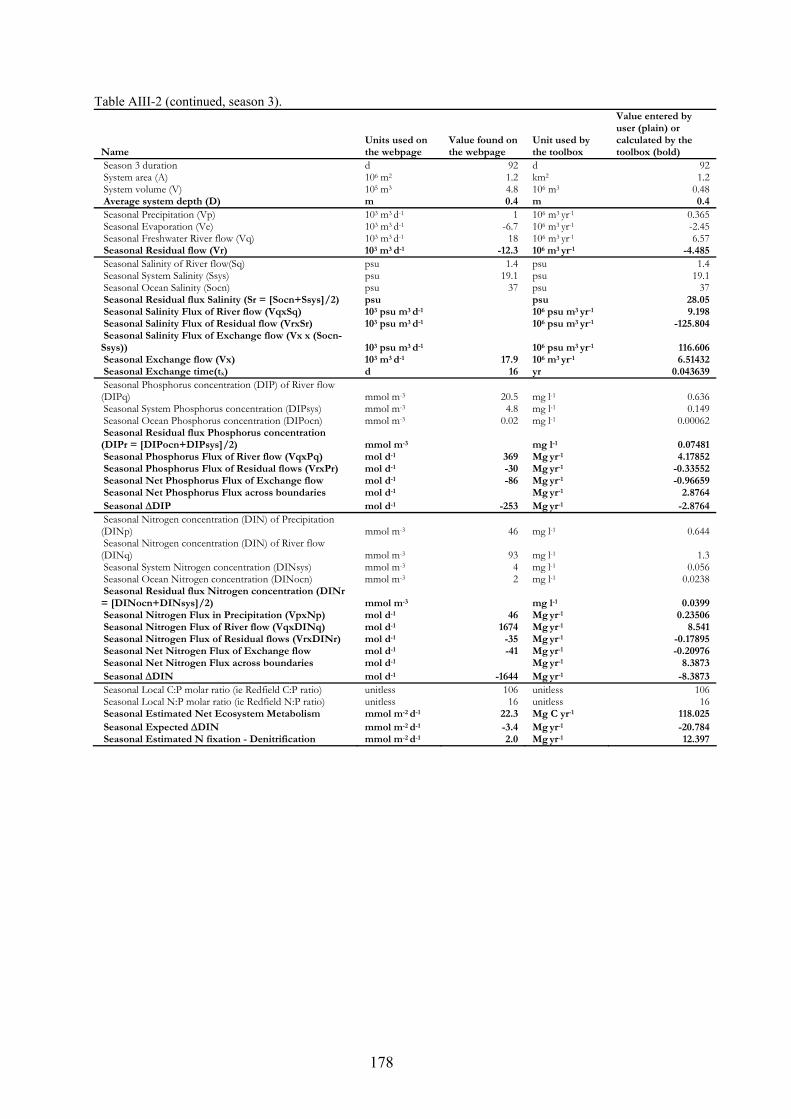
178






Season 3 duration d 92 d 92 System area (A) 106 m2 1.2 km2 1.2 System volume (V) 105 m3 4.8 106 m3 0.48 Average system depth (D) m 0.4 m 0.4 Seasonal Precipitation (Vp) 103 m3 d-1 1 106 m3 yr-1 0.365 Seasonal Evaporation (Ve) 103 m3 d-1 -6.7 106 m3 yr-1 -2.45 Seasonal Freshwater River flow (Vq) 103 m3 d-1 18 106 m3 yr-1 6.57 Seasonal Residual flow (Vr) 103 m3 d-1 -12.3 106 m3 yr-1 -4.485 Seasonal Salinity of River flow(Sq) psu 1.4 psu 1.4 Seasonal System Salinity (Ssys) psu 19.1 psu 19.1 Seasonal Ocean Salinity (Socn) psu 37 psu 37 Seasonal Residual flux Salinity (Sr = [Socn+Ssys]/2) psu psu 28.05 Seasonal Salinity Flux of River flow (VqxSq) 103 psu m3 d-1 106 psu m3 yr-1 9.198 Seasonal Salinity Flux of Residual flow (VrxSr) 103 psu m3 d-1 106 psu m3 yr-1 -125.804 Seasonal Salinity Flux of Exchange flow (Vx x (Socn-Ssys)) 103 psu m3 d-1 106 psu m3 yr-1 116.606 Seasonal Exchange flow (Vx) 103 m3 d-1 17.9 106 m3 yr-1 6.51432 Seasonal Exchange time(tx) d 16 yr 0.043639 Seasonal Phosphorus concentration (DIP) of River flow (DIPq) mmol m-3 20.5 mg l-1 0.636 Seasonal System Phosphorus concentration (DIPsys) mmol m-3 4.8 mg l-1 0.149 Seasonal Ocean Phosphorus concentration (DIPocn) mmol m-3 0.02 mg l-1 0.00062 Seasonal Residual flux Phosphorus concentration (DIPr = [DIPocn+DIPsys]/2) mmol m-3 mg l-1 0.07481 Seasonal Phosphorus Flux of River flow (VqxPq) mol d-1 369 Mg yr-1 4.17852 Seasonal Phosphorus Flux of Residual flows (VrxPr) mol d-1 -30 Mg yr-1 -0.33552 Seasonal Net Phosphorus Flux of Exchange flow mol d-1 -86 Mg yr-1 -0.96659 Seasonal Net Phosphorus Flux across boundaries mol d-1 Mg yr-1 2.8764 Seasonal ΔDIP mol d-1 -253 Mg yr-1 -2.8764 Seasonal Nitrogen concentration (DIN) of Precipitation (DINp) mmol m-3 46 mg l-1 0.644 Seasonal Nitrogen concentration (DIN) of River flow (DINq) mmol m-3 93 mg l-1 1.3 Seasonal System Nitrogen concentration (DINsys) mmol m-3 4 mg l-1 0.056 Seasonal Ocean Nitrogen concentration (DINocn) mmol m-3 2 mg l-1 0.0238 Seasonal Residual flux Nitrogen concentration (DINr = [DINocn+DINsys]/2) mmol m-3 mg l-1 0.0399 Seasonal Nitrogen Flux in Precipitation (VpxNp) mol d-1 46 Mg yr-1 0.23506 Seasonal Nitrogen Flux of River flow (VqxDINq) mol d-1 1674 Mg yr-1 8.541 Seasonal Nitrogen Flux of Residual flows (VrxDINr) mol d-1 -35 Mg yr-1 -0.17895 Seasonal Net Nitrogen Flux of Exchange flow mol d-1 -41 Mg yr-1 -0.20976 Seasonal Net Nitrogen Flux across boundaries mol d-1 Mg yr-1 8.3873 Seasonal ΔDIN mol d-1 -1644 Mg yr-1 -8.3873 Seasonal Local C:P molar ratio (ie Redfield C:P ratio) unitless 106 unitless 106 Seasonal Local N:P molar ratio (ie Redfield N:P ratio) unitless 16 unitless 16 Seasonal Estimated Net Ecosystem Metabolism mmol m-2 d-1 22.3 Mg C yr-1 118.025 Seasonal Expected ΔDIN mmol m-2 d-1 -3.4 Mg yr-1 -20.784 Seasonal Estimated N fixation - Denitrification mmol m-2 d-1 2.0 Mg yr-1 12.397

179






Season 4 duration d 92 d 92 System area (A) 106 m2 1.2 km2 1.2 System volume (V) 105 m3 4.8 106 m3 0.48 Average system depth (D) m 0.4 m 0.4 Seasonal Precipitation (Vp) 103 m3 d-1 3.6 106 m3 yr-1 1.31 Seasonal Evaporation (Ve) 103 m3 d-1 -2.5 106 m3 yr-1 -0.913 Seasonal Freshwater River flow (Vq) 103 m3 d-1 58.7 106 m3 yr-1 21.4 Seasonal Residual flow (Vr) 103 m3 d-1 -59.8 106 m3 yr-1 -21.797 Seasonal Salinity of River flow(Sq) psu 1.8 psu 1.8 Seasonal System Salinity (Ssys) psu 21.3 psu 21.3 Seasonal Ocean Salinity (Socn) psu 37 psu 37 Seasonal Residual flux Salinity (Sr = [Socn+Ssys]/2) psu psu 29.15 Seasonal Salinity Flux of River flow (VqxSq) 103 psu m3 d-1 106 psu m3 yr-1 38.52 Seasonal Salinity Flux of Residual flow (VrxSr) 103 psu m3 d-1 106 psu m3 yr-1 -635.38 Seasonal Salinity Flux of Exchange flow (Vx x (Socn-Ssys)) 103 psu m3 d-1 106 psu m3 yr-1 596.86 Seasonal Exchange flow (Vx) 103 m3 d-1 104.5 106 m3 yr-1 38.017 Seasonal Exchange time(tx) d 3 yr 0.008025 Seasonal Phosphorus concentration (DIP) of River flow (DIPq) mmol m-3 19.4 mg l-1 0.601 Seasonal System Phosphorus concentration (DIPsys) mmol m-3 2.6 mg l-1 0.0806 Seasonal Ocean Phosphorus concentration (DIPocn) mmol m-3 0.02 mg l-1 0.00062 Seasonal Residual flux Phosphorus concentration (DIPr = [DIPocn+DIPsys]/2) mmol m-3 mg l-1 0.04061 Seasonal Phosphorus Flux of River flow (VqxPq) mol d-1 1139 Mg yr-1 12.861 Seasonal Phosphorus Flux of Residual flows (VrxPr) mol d-1 -78 Mg yr-1 -0.88518 Seasonal Net Phosphorus Flux of Exchange flow mol d-1 -270 Mg yr-1 -3.0406 Seasonal Net Phosphorus Flux across boundaries mol d-1 Mg yr-1 8.9356 Seasonal ΔDIP mol d-1 -791 Mg yr-1 -8.9356 Seasonal Nitrogen concentration (DIN) of Precipitation (DINp) mmol m-3 46 mg l-1 0.644 Seasonal Nitrogen concentration (DIN) of River flow (DINq) mmol m-3 128 mg l-1 1.79 Seasonal System Nitrogen concentration (DINsys) mmol m-3 3 mg l-1 0.042 Seasonal Ocean Nitrogen concentration (DINocn) mmol m-3 2 mg l-1 0.0238 Seasonal Residual flux Nitrogen concentration (DINr = [DINocn+DINsys]/2) mmol m-3 mg l-1 0.0329 Seasonal Nitrogen Flux in Precipitation (VpxNp) mol d-1 166 Mg yr-1 0.84364 Seasonal Nitrogen Flux of River flow (VqxDINq) mol d-1 7514 Mg yr-1 38.306 Seasonal Nitrogen Flux of Residual flows (VrxDINr) mol d-1 -141 Mg yr-1 -0.71712 Seasonal Net Nitrogen Flux of Exchange flow mol d-1 -136 Mg yr-1 -0.6919 Seasonal Net Nitrogen Flux across boundaries mol d-1 Mg yr-1 37.741 Seasonal ΔDIN mol d-1 -7403 Mg yr-1 -37.741 Seasonal Local C:P molar ratio (ie Redfield C:P ratio) unitless 106 unitless 106 Seasonal Local N:P molar ratio (ie Redfield N:P ratio) unitless 16 unitless 16 Seasonal Estimated Net Ecosystem Metabolism mmol m-2 d-1 70 Mg C yr-1 366.65 Seasonal Expected ΔDIN mmol m-2 d-1 -10.6 Mg yr-1 -64.567 Seasonal Estimated N fixation - Denitrification mmol m-2 d-1 4.4 Mg yr-1 26.827

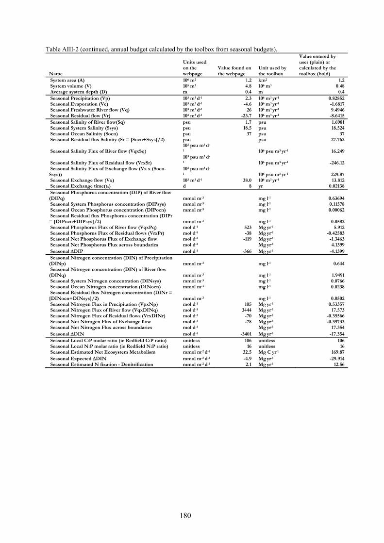
180

Table AIII-2 (continued, annual budget calculated by the toolbox from seasonal budgets).

Name





System area (A) 106 m2 1.2 km2 1.2 System volume (V) 105 m3 4.8 106 m3 0.48 Average system depth (D) m 0.4 m 0.4 Seasonal Precipitation (Vp) 103 m3 d-1 2.3 106 m3 yr-1 0.82852 Seasonal Evaporation (Ve) 103 m3 d-1 -4.6 106 m3 yr-1 -1.6817 Seasonal Freshwater River flow (Vq) 103 m3 d-1 26 106 m3 yr-1 9.4946 Seasonal Residual flow (Vr) 103 m3 d-1 -23.7 106 m3 yr-1 -8.6415 Seasonal Salinity of River flow(Sq) psu 1.7 psu 1.6981 Seasonal System Salinity (Ssys) psu 18.5 psu 18.524 Seasonal Ocean Salinity (Socn) psu 37 psu 37 Seasonal Residual flux Salinity (Sr = [Socn+Ssys]/2) psu psu 27.762

Seasonal Salinity Flux of River flow (VqxSq) 103 psu m3 d-

1 106 psu m3 yr-1 16.249

Seasonal Salinity Flux of Residual flow (VrxSr) 103 psu m3 d-

1 106 psu m3 yr-1 -246.12 Seasonal Salinity Flux of Exchange flow (Vx x (Socn-Ssys))

103 psu m3 d-

1 106 psu m3 yr-1 229.87 Seasonal Exchange flow (Vx) 103 m3 d-1 38.0 106 m3 yr-1 13.812 Seasonal Exchange time(tx) d 8 yr 0.02138 Seasonal Phosphorus concentration (DIP) of River flow (DIPq) mmol m-3 mg l-1 0.63694 Seasonal System Phosphorus concentration (DIPsys) mmol m-3 mg l-1 0.11578 Seasonal Ocean Phosphorus concentration (DIPocn) mmol m-3 mg l-1 0.00062 Seasonal Residual flux Phosphorus concentration (DIPr = [DIPocn+DIPsys]/2) mmol m-3 mg l-1 0.0582 Seasonal Phosphorus Flux of River flow (VqxPq) mol d-1 523 Mg yr-1 5.912 Seasonal Phosphorus Flux of Residual flows (VrxPr) mol d-1 -38 Mg yr-1 -0.42583 Seasonal Net Phosphorus Flux of Exchange flow mol d-1 -119 Mg yr-1 -1.3463 Seasonal Net Phosphorus Flux across boundaries mol d-1 Mg yr-1 4.1399 Seasonal ΔDIP mol d-1 -366 Mg yr-1 -4.1399 Seasonal Nitrogen concentration (DIN) of Precipitation (DINp) mmol m-3 mg l-1 0.644 Seasonal Nitrogen concentration (DIN) of River flow (DINq) mmol m-3 mg l-1 1.9491 Seasonal System Nitrogen concentration (DINsys) mmol m-3 mg l-1 0.0766 Seasonal Ocean Nitrogen concentration (DINocn) mmol m-3 mg l-1 0.0238 Seasonal Residual flux Nitrogen concentration (DINr = [DINocn+DINsys]/2) mmol m-3 mg l-1 0.0502 Seasonal Nitrogen Flux in Precipitation (VpxNp) mol d-1 105 Mg yr-1 0.53357 Seasonal Nitrogen Flux of River flow (VqxDINq) mol d-1 3444 Mg yr-1 17.573 Seasonal Nitrogen Flux of Residual flows (VrxDINr) mol d-1 -70 Mg yr-1 -0.35566 Seasonal Net Nitrogen Flux of Exchange flow mol d-1 -78 Mg yr-1 -0.39733 Seasonal Net Nitrogen Flux across boundaries mol d-1 Mg yr-1 17.354 Seasonal ΔDIN mol d-1 -3401 Mg yr-1 -17.354 Seasonal Local C:P molar ratio (ie Redfield C:P ratio) unitless 106 unitless 106 Seasonal Local N:P molar ratio (ie Redfield N:P ratio) unitless 16 unitless 16 Seasonal Estimated Net Ecosystem Metabolism mmol m-2 d-1 32.5 Mg C yr-1 169.87 Seasonal Expected ΔDIN mmol m-2 d-1 -4.9 Mg yr-1 -29.914 Seasonal Estimated N fixation - Denitrification mmol m-2 d-1 2.1 Mg yr-1 12.56

181

Figure AIII-6. Tabulated budget for S’Ena Arrubia lagoon, Italy (season 1).


182



183

Figure AIII-10. Annual water budget diagram for S’Ena Arrubia lagoon, Italy.

Figure AIII-11. Annual salt budget diagram for S’Ena Arrubia lagoon, Italy.

184

Figure AIII-12. Annual phosphorus budget diagram for S’Ena Arrubia lagoon, Italy.

Figure AIII-13. Annual phosphorus budget diagram for S’Ena Arrubia lagoon, Italy.

185

3. Example of a Multiple Compartment Model This example is from the Mandovi estuary, Goa, India. The data describing this system can be found at http://nest.su.se/mnode/Asia/India/Mandovi/Mandovibud.htm. Out of the three seasons (pre-monsoon, monsoon, and post-monsoon) available on the web, only the first season data are used as a demonstration of the multiple compartment model. To try out this example: (1) set the number of compartments to 3, the number of seasons to 1, and the number of layers to 1 in the “Instructions and basic info” worksheet, (2) set all the unit options to 2 (the user may choose their own unit options if desired), (3) click on “LOICZ budgets > Create budget template” to create a budget template worksheet “Annual”, (4) fill out the light yellow cells in the “Annual” worksheet using the values in Table AIII-3, (5) click on “LOICZ budgets > Generate budget tables > Create tables for all compartments and seasons” to generate budget tables (Figures AIII-14 – AIII-16), and (6) click on “LOICZ budgets > Generate budget diagrams > Create diagrams for all compartments and seasons” to create budget diagrams (Figure AIII-17 – AIII-20). Table AIII-3. Example of Mandovi estuary, Goa, India (compartment 1).

Name





compartment 1 System area (A) km2 3 km2 3 compartment 1 System volume (V) 106 m3 6 106 m3 6 compartment 1 Average system depth (D) m m 2compartment 1 Annual Precipitation (Vp) 103 m3 d-1 1 106 m3 yr-1 0.365compartment 1 Annual Evaporation (Ve) 103 m3 d-1 -9 106 m3 yr-1 -3.29compartment 1 Annual Freshwater River flow (Vq) 103 m3 d-1 160 106 m3 yr-1 58.4compartment 1 Annual Residual flow (Vr) 103 m3 d-1 -152 106 m3 yr-1 -55.475compartment 1 Annual System Salinity (Ssys) psu 6.7 psu 6.7compartment 1 Annual Ocean Salinity (Socn) psu 31.7 psu 31.7compartment 1 Annual Residual flux Salinity (Sr = [Socn+Ssys]/2) psu psu 19.2

compartment 1 Annual Salinity Flux of Residual flow (VrxSr) 103 psu m3 d-

1 106 psu m3 yr-1 -1065.1compartment 1 Annual Salinity Flux of Exchange flow (Vx x (Socn-Ssys))

103 psu m3 d-

1 106 psu m3 yr-1 1065.1compartment 1 Annual Exchange flow (Vx) 103 m3 d-1 117 106 m3 yr-1 42.605compartment 1 Annual Exchange time(tx) d 22 yr 0.06117compartment 1 Annual Phosphorus concentration (DIP) of River flow (DIPq) mmol m-3 0.8 mg l-1 0.0248compartment 1 Annual System Phosphorus concentration (DIPsys) mmol m-3 0.2 mg l-1 0.0062compartment 1 Annual Ocean Phosphorus concentration (DIPocn) mmol m-3 0.6 mg l-1 0.0186compartment 1 Annual Residual flux Phosphorus concentration (DIPr = [DIPocn+DIPsys]/2) mmol m-3 mg l-1 0.0124compartment 1 Annual Phosphorus Flux of River flow (VqxPq) mol d-1 128 Mg yr-1 1.4483compartment 1 Annual Phosphorus Flux of Residual flows (VrxPr) mol d-1 -61 Mg yr-1 -0.68789compartment 1 Annual Net Phosphorus Flux of Exchange flow mol d-1 47 Mg yr-1 0.5283compartment 1 Annual Net Phosphorus Flux across boundaries mol d-1 Mg yr-1 1.2887compartment 1 Annual ΔDIP mol d-1 -114 Mg yr-1 -1.2887compartment 1 Annual Nitrogen concentration (DIN) of Precipitation (DINp) mmol m-3 2.0 mg l-1 0.028compartment 1 Annual Nitrogen concentration (DIN) of River flow (DINq) mmol m-3 3.1 mg l-1 0.0434compartment 1 Annual System Nitrogen concentration (DINsys) mmol m-3 2.1 mg l-1 0.0294compartment 1 Annual Ocean Nitrogen concentration (DINocn) mmol m-3 1.8 mg l-1 0.0252compartment 1 Annual Residual flux Nitrogen concentration (DINr = [DINocn+DINsys]/2) mmol m-3 mg l-1 0.0273compartment 1 Annual Nitrogen Flux in Precipitation (VpxNp) mol d-1 2 Mg yr-1 0.01022compartment 1 Annual Nitrogen Flux of River flow (VqxDINq) mol d-1 496 Mg yr-1 2.5346compartment 1 Annual Nitrogen Flux of Residual flows (VrxDINr) mol d-1 -296 Mg yr-1 -1.5145compartment 1 Annual Net Nitrogen Flux of Exchange flow mol d-1 -35 Mg yr-1 -0.17894compartment 1 Annual Net Nitrogen Flux across boundaries mol d-1 Mg yr-1 0.85137compartment 1 Annual ΔDIN mol d-1 -167 Mg yr-1 -0.85137compartment 1 Annual Local C:P molar ratio (ie Redfield C:P ratio) unitless 106 unitless 106compartment 1 Annual Local N:P molar ratio (ie Redfield N:P ratio) unitless 16 unitless 16compartment 1 Annual Estimated Net Ecosystem Metabolism mmol m-2 d-1 4 Mg C yr-1 52.879compartment 1 Annual Expected ΔDIN mmol m-2 d-1 Mg yr-1 -9.3121compartment 1 Annual Estimated N fixation - Denitrification mmol m-2 d-1 0.6 Mg yr-1 8.4607

186

Table AIII-3 (continued, compartment 2).

Name





compartment 2 System area (A) km2 10 km2 10compartment 2 System volume (V) 106 m3 30 106 m3 30compartment 2 Average system depth (D) m m 3compartment 2 Annual Precipitation (Vp) 103 m3 d-1 4 106 m3 yr-1 1.46compartment 2 Annual Evaporation (Ve) 103 m3 d-1 -30 106 m3 yr-1 -11compartment 2 Annual Residual flow (Vr) 103 m3 d-1 126 106 m3 yr-1 -45.935compartment 2 Annual Upstream Residual flow (Vr) 103 m3 d-1 106 m3 yr-1 55.475compartment 2 Annual Upstream Exchange flow (Vx) 103 m3 d-1 106 m3 yr-1 42.605compartment 2 Annual System Salinity (Ssys) psu 31.7 psu 31.7compartment 2 Annual Ocean Salinity (Socn) psu 35.4 psu 35.4compartment 2 Annual Residual flux Salinity (Sr = [Socn+Ssys]/2) psu psu 33.55

compartment 2 Annual Salinity Flux of Residual flow (VrxSr) 103 psu m3 d-

1 106 psu m3 yr-1 -1541.1compartment 2 Annual Salinity Flux of Exchange flow (Vx x (Socn-Ssys))

103 psu m3 d-

1 106 psu m3 yr-1 1541.1compartment 2 Annual Exchange flow (Vx) 103 m3 d-1 1142 106 m3 yr-1 416.52compartment 2 Annual Exchange time(tx) d 22 yr 0.0594compartment 2 Annual System Phosphorus concentration (DIPsys) mmol m-3 0.6 mg l-1 0.0186compartment 2 Annual Ocean Phosphorus concentration (DIPocn) mmol m-3 0.6 mg l-1 0.0186compartment 2 Annual Residual flux Phosphorus concentration (DIPr = [DIPocn+DIPsys]/2) mmol m-3 mg l-1 0.0186compartment 2 Annual Phosphorus Flux of Residual flows (VrxPr) mol d-1 -76 Mg yr-1 -0.85439compartment 2 Annual Net Phosphorus Flux across boundaries mol d-1 Mg yr-1 -0.6948compartment 2 Annual ΔDIP mol d-1 62 Mg yr-1 0.6948compartment 2 Annual Nitrogen concentration (DIN) of Precipitation (DINp) mmol m-3 2.0 mg l-1 0.028compartment 2 Annual System Nitrogen concentration (DINsys) mmol m-3 1.8 mg l-1 0.0252compartment 2 Annual Ocean Nitrogen concentration (DINocn) mmol m-3 1.4 mg l-1 0.0196compartment 2 Annual Residual flux Nitrogen concentration (DINr = [DINocn+DINsys]/2) mmol m-3 mg l-1 0.0224compartment 2 Annual Nitrogen Flux in Precipitation (VpxNp) mol d-1 8 Mg yr-1 0.04088compartment 2 Annual Nitrogen Flux of Residual flows (VrxDINr) mol d-1 -202 Mg yr-1 -1.0289compartment 2 Annual Net Nitrogen Flux of Exchange flow mol d-1 -457 Mg yr-1 -2.3325compartment 2 Annual Net Nitrogen Flux across boundaries mol d-1 Mg yr-1 -1.6272compartment 2 Annual ΔDIN mol d-1 320 Mg yr-1 1.6272compartment 2 Annual Local C:P molar ratio (ie Redfield C:P ratio) unitless 106 unitless 106compartment 2 Annual Local N:P molar ratio (ie Redfield N:P ratio) unitless 16 unitless 16compartment 2 Annual Estimated Net Ecosystem Metabolism mmol m-2 d-1 -1 Mg C yr-1 -28.509compartment 2 Annual Expected ΔDIN mmol m-2 d-1 Mg yr-1 5.0205compartment 2 Annual Estimated N fixation - Denitrification mmol m-2 d-1 -0.1 Mg yr-1 -3.3933

187

Table AIII-3 (continued, compartment 3).

Name





compartment 3 System area (A) km2 16 km2 16compartment 3 System volume (V) 106 m3 80 106 m3 80compartment 3 Average system depth (D) m m 5compartment 3 Annual Precipitation (Vp) 103 m3 d-1 7 106 m3 yr-1 2.56compartment 3 Annual Evaporation (Ve) 103 m3 d-1 -48 106 m3 yr-1 -17.5compartment 3 Annual Other Freshwater flows (Vo) 103 m3 d-1 7 106 m3 yr-1 2.56compartment 3 Annual Residual flow (Vr) 103 m3 d-1 -92 106 m3 yr-1 -33.555compartment 3 Annual Upstream Residual flow (Vr) 103 m3 d-1 106 m3 yr-1 45.935compartment 3 Annual Upstream Exchange flow (Vx) 103 m3 d-1 106 m3 yr-1 416.52compartment 3 Annual System Salinity (Ssys) psu 35.4 psu 35.4compartment 3 Annual Ocean Salinity (Socn) psu 36.3 psu 36.3compartment 3 Annual Residual flux Salinity (Sr = [Socn+Ssys]/2) psu psu 35.85compartment 3 Annual Salinity Flux of Residual flow (VrxSr) 103 psu m3 d-1 106 psu m3 yr-1 -1202.9compartment 3 Annual Salinity Flux of Exchange flow (Vx x (Socn-Ssys)) 103 psu m3 d-1 106 psu m3 yr-1 1202.9compartment 3 Annual Exchange flow (Vx) 103 m3 d-1 3664 106 m3 yr-1 1336.6compartment 3 Annual Exchange time(tx) d 16 yr 0.04478compartment 3 Annual Phosphorus concentration of Other Freshwater flows (DIPo) mmol m-3 160 mg l-1 4.96compartment 3 Annual System Phosphorus concentration (DIPsys) mmol m-3 0.6 mg l-1 0.0186compartment 3 Annual Ocean Phosphorus concentration (DIPocn) mmol m-3 1.3 mg l-1 0.0403compartment 3 Annual Residual flux Phosphorus concentration (DIPr = [DIPocn+DIPsys]/2) mmol m-3 mg l-1 0.02945compartment 3 Annual Phosphorus Flux of Other Freshwater flows (VoxPo) mol d-1 1120 Mg yr-1 12.698compartment 3 Annual Phosphorus Flux of Residual flows (VrxPr) mol d-1 -87 Mg yr-1 -0.98819compartment 3 Annual Net Phosphorus Flux of Exchange flow mol d-1 2565 Mg yr-1 29.004compartment 3 Annual Net Phosphorus Flux across boundaries mol d-1 Mg yr-1 41.568compartment 3 Annual ΔDIP mol d-1 -3674 Mg yr-1 -41.568compartment 3 Annual Nitrogen concentration (DIN) of Precipitation (DINp) mmol m-3 2.0 mg l-1 0.028compartment 3 Annual Nitrogen concentration of Other Freshwater flows (DINo) mmol m-3 3600 mg l-1 50.4compartment 3 Annual System Nitrogen concentration (DINsys) mmol m-3 1.4 mg l-1 0.0196compartment 3 Annual Ocean Nitrogen concentration (DINocn) mmol m-3 7.2 mg l-1 0.101compartment 3 Annual Residual flux Nitrogen concentration (DINr = [DINocn+DINsys]/2) mmol m-3 mg l-1 0.0603compartment 3 Annual Nitrogen Flux in Precipitation (VpxNp) mol d-1 14 Mg yr-1 0.0717compartment 3 Annual Nitrogen Flux of Other Freshwater flows (VoxDINo) mol d-1 25200 Mg yr-1 129.02compartment 3 Annual Nitrogen Flux of Residual flows (VrxDINr) mol d-1 -396 Mg yr-1 -2.0234compartment 3 Annual Net Nitrogen Flux of Exchange flow mol d-1 21251 Mg yr-1 108.8compartment 3 Annual Net Nitrogen Flux across boundaries mol d-1 Mg yr-1 239.23compartment 3 Annual ΔDIN mol d-1 -46728 Mg yr-1 -239.23compartment 3 Annual Local C:P molar ratio (ie Redfield C:P ratio) unitless 106 unitless 106compartment 3 Annual Local N:P molar ratio (ie Redfield N:P ratio) unitless 16 unitless 16compartment 3 Annual Estimated Net Ecosystem Metabolism mmol m-2 d-1 24 Mg C yr-1 1705.6compartment 3 Annual Expected ΔDIN mmol m-2 d-1 Mg yr-1 -300.36compartment 3 Annual Estimated N fixation - Denitrification mmol m-2 d-1 0.8 Mg yr-1 61.13

188

Figure AIII-14. Tabulated budget for Mandovi Estuary, Goa, India (compartment 1).


189


Figure AIII-17. Water budget diagram for Mandovi Estuary, Goa, India.

190

Figure AIII-18. Salt budget diagram for Mandovi Estuary, Goa, India.

Figure AIII-19. Phosphorus budget diagram for Mandovi Estuary, Goa, India.

Figure AIII-20. Nitrogen budget diagram for Mandovi Estuary, Goa, India.

191

4. Example of a Two Layer Model This example is from the ThuBon River estuary, Vietnam. The data describing this system can be found at http://nest.su.se/mnode/Asia/Vietnam/ThuBon/thubonbud.htm. To try out this example: (1) set the number of compartments to 1, the number of seasons to 1, and the number of layers to 2 in the “Instructions and basic info” worksheet, (2) set all the unit options to 2 (the user may choose their own unit options if desired), (3) click on “LOICZ budgets > Create budget template” to create a budget template worksheet “Annual”, (4) fill out the light yellow cells in the “Annual” worksheet using the values in Table AIII-4, (5) click on “LOICZ budgets > Generate budget tables > Create tables for all compartments and seasons” to generate budget tables (Figures AIII-21 – AIII-22), and (6) click on “LOICZ budgets > Generate budget diagrams > Create diagrams for all compartments and seasons” to create budget diagrams (Figure AIII-23 – AIII-26). Table AIII-4. Example of ThuBon River estuary, Vietnam (top layer).




Value entered (plain) or calculated by toolbox (bold)

layer 1 System area (A) km2 12 km2 12layer 1 System volume (V) 106 m3 106 m3 25layer 1 Average system depth (D) m m 2.0833layer 1 Annual Freshwater River flow (Vq) 106 m3 d-1 10 106 m3 yr-1 3650layer 1 Annual Residual flow (Vr) 106 m3 d-1 106 m3 yr-1 -3650layer 1 Annual Surface Layer System Salinity (Ssys) psu 4.7 psu 4.7layer 1 Annual Surface Layer Ocean Salinity (Socn) psu 31.5 psu 31.5layer 1 Annual Residual flux Salinity (Sr = Ssyss) psu psu 4.7layer 1 Annual Salinity Flux of vertical flow (VdeepxSdeep) 106 psu m3 d-1 50 106 psu m3 yr-1 17731.1layer 1 Annual Salinity Flux of surface flow (VsurfxSsurf) 103 psu m3 d-1 -56 106 psu m3 yr-1 -20163.5layer 1 Annual Vertical flow (Vdeep) 106 m3 d-1 1.8 106 m3 yr-1 640.11layer 1 Annual Vertical exchange flow (Vz) 106 m3 d-1 0.3 106 m3 yr-1 105.76layer 1 Annual Surface flow to sea (Vsurf) 106 m3 d-1 -12 106 m3 yr-1 -4290.1layer 1 Annual Exchange time(tx) d yr 0.005687layer 1 Annual Salinity Flux of exchange flow (VzxSz) 106 psu m3 d-1 6 106 psu m3 yr-1 2432.4layer 1 Annual Phosphorus concentration (DIP) of River flow (DIPq) mmol m-3 32.4 mg l-1 1.004layer 1 Annual Surface Layer System Phosphorus concentration (DIPsys) mmol m-3 1.4 mg l-1 0.0434layer 1 Annual Surface Layer Ocean Phosphorus concentration (DIPocn) mmol m-3 0.1 mg l-1 0.0031layer 1 Annual Residual flux Phosphorus concentration (DIPr = DIPsyss) mmol m-3 mg l-1 0.0434layer 1 Annual Phosphorus Flux of River flow (VqxPq) 103 mol d-1 324 Mg yr-1 3664.6layer 1 Annual Phosphorus Flux of Vsurf (VsurfxDIPsys) 103 mol d-1 -17 Mg yr-1 -186.19layer 1 Annual Net Phosphorus Flux of Vz 103 mol d-1 0 Mg yr-1 -3.9342layer 1 Annual Phosphorus Flux of Vdeep 103 mol d-1 0 Mg yr-1 3.9687layer 1 Annual Net Phosphorus Flux across boundaries 103 mol d-1 Mg yr-1 3478.4layer 1 Annual ΔDIP 103 mol d-1 -307 Mg yr-1 -3478.4layer 1 Annual Nitrogen concentration (DIN) of River flow (DINq) mmol m-3 87.5 mg l-1 1.23layer 1 Annual Surface Layer System Nitrogen concentration (DINsys) mmol m-3 8.7 mg l-1 0.122layer 1 Annual Surface Layer Ocean Nitrogen concentration (DINocn) mmol m-3 19.6 mg l-1 0.274layer 1 Annual Residual flux Nitrogen concentration (DINr = DINsyss) mmol m-3 mg l-1 0.122layer 1 Annual Nitrogen Flux of River flow (VqxDINq) 103 mol d-1 875 Mg yr-1 4489.5layer 1 Annual Nitrogen Flux of Vsurf (VsurfxDINsys) 103 mol d-1 -104 Mg yr-1 -523.39layer 1 Annual Net Nitrogen Flux of Vz 103 mol d-1 2 Mg yr-1 11.633layer 1 Annual Nitrogen Flux of Vdeep 103 mol d-1 30 Mg yr-1 148.51layer 1 Annual Net Nitrogen Flux across boundaries 103 mol d-1 Mg yr-1 4126.2layer 1 Annual ΔDIN 103 mol d-1 -803 Mg yr-1 -4126.2layer 1 Annual Local C:P molar ratio (ie Redfield C:P ratio) unitless 106 unitless 106layer 1 Annual Local N:P molar ratio (ie Redfield N:P ratio) unitless 16 unitless 16layer 1 Annual Estimated Net Ecosystem Metabolism 103 mol C d-1 3254 Mg C yr-1 142728.4layer 1 Annual Estimated Net Ecosystem Metabolism (Standard Unit)

mmol C m-2 d-

1 mmol C m-2 d-1 2715.5layer 1 Annual Expected ΔDIN 103 mol N d-1 -4912 Mg yr-1 -25134.6layer 1 Annual Estimated N fixation - Denitrification (Standard Unit) mmol m-2 d-1 mmol m-2 d-1 342.6layer 1 Annual Estimated N fixation - Denitrification 103 mol N d-1 4109 Mg yr-1 21008.3

192

Table AIII-4 (continued, bottom layer).





layer 2 System area (A) km2 12 km2 12layer 2 System volume (V) 106 m3 106 m3 25layer 2 Average system depth (D) m m 2.0833layer 2 AnnualDeep Layer System Salinity (Ssys) psu 27.7 psu 27.7layer 2 AnnualDeep Layer Ocean Salinity (Socn) psu 31.5 psu 31.5layer 2 Annual Residual flux Salinity (Sdeep = Ssys) psu psu 27.7layer 2 Annual Salinity Flux of Vdeep from ocean (VdeepxSocn) 106 psu m3 d-1 56 106 psu m3 yr-1 20163.5layer 2 Annual Vertical flow (Vdeep) 106 m3 d-1 -1.8 106 m3 yr-1 -640.11layer 2 Annual Vertical exchange flow (Vz) 106 m3 d-1 0.3 106 m3 yr-1 105.76layer 2 Annual Vdeep flow from ocean (Vb) 106 m3 d-1 1.8 106 m3 yr-1 640.11layer 2 Annual Exchange time(tx) d yr 0.03352layer 2 AnnualDeep Layer System Phosphorus concentration (DIPsys) mmol m-3 0.2 mg l-1 0.0062layer 2 AnnualDeep Layer Ocean Phosphorus concentration (DIPocn) mmol m-3 0.1 mg l-1 0.0031layer 2 Annual Residual flux Phosphorus concentration (DIPdeep = DIPsysd) mmol m-3 mg l-1 0.0062layer 2 Annual Phosphorus Flux of Vdeep from ocean (VdeepxDIPod) 103 mol d-1 0 Mg yr-1 1.9843layer 2 Annual Net Phosphorus Flux of Vz to layer 1 103 mol d-1 0 Mg yr-1 3.9342layer 2 Annual Phosphorus Flux of Vdeep to layer 1 103 mol d-1 0 Mg yr-1 -3.9687layer 2 Annual Net Phosphorus Flux across boundaries 103 mol d-1 Mg yr-1 1.9498layer 2 Annual ΔDIP 103 mol d-1 0 Mg yr-1 -1.9498layer 2 AnnualDeep Layer System Nitrogen concentration (DINsys) mmol m-3 16.6 mg l-1 0.232layer 2 AnnualDeep Layer Ocean Nitrogen concentration (DINocn) mmol m-3 19.6 mg l-1 0.274layer 2 Annual Residual flux Nitrogen concentration (DINdeep = DINsysd) mmol m-3 mg l-1 0.232layer 2 Annual Nitrogen Flux of Vdeep from ocean (VdeepxDINod) 103 mol d-1 35 Mg yr-1 175.39layer 2 Annual Net Nitrogen Flux of Vz to layer 1 103 mol d-1 -2 Mg yr-1 -11.633layer 2 Annual Nitrogen Flux of Vdeep to layer 1 103 mol d-1 -30 Mg yr-1 -148.51layer 2 Annual Net Nitrogen Flux across boundaries 103 mol d-1 Mg yr-1 15.251layer 2 Annual ΔDIN 103 mol d-1 -3 Mg yr-1 -15.251layer 2 Annual Local C:P molar ratio (ie Redfield C:P ratio) unitless 106 unitless 106layer 2 Annual Local N:P molar ratio (ie Redfield N:P ratio) unitless 16 unitless 16layer 2 Annual Estimated Net Ecosystem Metabolism 103 mol C d-1 0 Mg C yr-1 80.006

layer 2 Annual Estimated Net Ecosystem Metabolism (Standard Unit) mmol C m-2 d-

1 mmol C m-2 d-1 1.5222layer 2 Annual Expected ΔDIN 103 mol N d-1 0 Mg yr-1 -14.089layer 2 Annual Estimated N fixation - Denitrification (Standard Unit) mmol m-2 d-1 mmol m-2 d-1 -0.01895layer 2 Annual Estimated N fixation - Denitrification 103 mol N d-1 -3 Mg yr-1 -1.1622

193

Figure AIII-21. Tabulated budget for ThuBon River estuary, Vietnam (surface layer).

Figure AIII-22. Tabulated budget for ThuBon River estuary, Vietnam (bottom layer).

194

Figure AIII-23. Water budget diagram for ThuBon River estuary, Vietnam.

Figure AIII-24. Salt budget diagram for ThuBon River estuary, Vietnam.

195

Figure AIII-25. Phosphorus budget diagram for ThuBon River estuary, Vietnam.

Figure AIII-26. Nitrogen budget diagram for ThuBon River estuary, Vietnam.