10th

World Congress on Structural and Multidisciplinary Optimization

May 19 -24, 2013, Orlando, Florida, USA

1

RSM Improvement Methods for Computationally Expensive Industrial CAE Analysis

Zhendan Xue1, Robert Lietz

2, Enrico Rigoni

3, Sumeet Parashar

1, Saket Kansara

4

1 Esteco North America, Novi, MI, USA

2 FORD Motor Company, Dearborn, MI, USA 3 Esteco SpA, Trieste, Italy

4 Esteco Software India pvt. ltd, Pune, Maharashtra, India

Abstract

Need for optimization in engineering design phase using computer simulations is now being widely

recognized, but its implementation practices vary depending on how expensive is the simulation involved

for objective and constraint function evaluation. Simulations of complex real-world problems using

in-house or commercial Computer Aided Engineering (CAE) software tools may take hours or even days to

compute. Due to this limitation, quite often these computationally expensive CAE simulations are not

directly employed in the iterative optimization strategies requiring hundreds or thousands of calculations.

Response Surface Models (RSM), also known as Surrogate Models are being increasingly used as

approximations of CAE models. As they are inexpensive to evaluate, RSMs prove to be very valuable in

optimization studies. It is obligatory to create a good quality RSM of a CAE model before using it in any

optimization study. In order to build a good quality RSM, training data set is typically created using Design

of Experiments (DoE) strategy which will spread the designs uniformly across the design space. However,

for expensive CAE problems with large number of design variables and non-linear responses, just a

uniform spread of points in design space may not provide an optimal training data. Adaptive/Sequential

DoE strategies can offer some advantage over such one-shot DoE strategies. This paper investigates the use

of such adaptive RSM strategies namely Multivariate Adaptive Crossvalidating Kriging (MACK) and

Lipschitz sampling and also a combination of these two with some incremental space filling DOE strategies.

This paper attempts to investigate various aspects related to practical application of such adaptive RSM

strategies such as: what should be the starting DoE population size before starting adaptive RSM iterations,

comparison of MACK and Lipschitz, whether adding designs using incremental space filling strategies

could be beneficial, what kind of error estimation metrics could be used for convergence check, effect of

number of design variables, and also how the strategies can take advantage of concurrent design

evaluations. The paper will also discuss MACK and Lipschitz strategies as implemented in the commercial

optimization software modeFRONTIER[1] and recent modifications to those algorithms to handle large

scale problems. The results of the application of above strategies applied to mathematical problems are

discussed. The primary problem of interest is to build a surrogate model of agreeable quality for

aerodynamic drag coefficient of passenger car where the shape of the passenger car is defined by 26 factors

/ design variables. Calculation of realistic drag coefficient values requires running a high fidelity

Computational Fluid Dynamics (CFD) model on high performance computing (HPC) machines and each

simulation can run of the order of 10-20 hours. The motivation for the work covered in this paper is to

investigate whether the adaptive RSM strategies can help to build a good quality RSM for drag coefficient

for problems of such scale, how many CFD simulations may be required, and whether it can be achieved

within reasonable time to fit the tight automotive design cycles while using HPC resources.

1. Introduction

Making optimization as part of standard design process has been slowly gaining acceptance over recent

years. Such transformation is facilitated by various factors such as increasing availability of computing power,

availability of commercial optimization software etc. These factors are considered important by the authors among

others because although optimization technology has been around for years, it was practiced mainly by the

research departments where people can write their own code and basic design teams where simulations (function

evaluations) are inexpensive. For production level design engineers who deal with expensive CAE (Computer

Aided Engineering) simulations such as finite element based structural analysis and computational fluid dynamics,

applying optimization is not trivial. Even today, when domain experts from the field such as external

aerodynamics apply optimization, they rely on optimization using surrogate models because running optimization

where every function evaluation can take of the order of 10 to 20 hours, just cannot fit into today’s tightly

scheduled automotive design cycles. The approach commonly employed in such areas consists of following steps:

2

run CAE simulations for a sufficiently large sample of configurations (designs) usually generated using a Design

of Experiment (DoE) algorithm, generate a response surface approximation or surrogate model using response

surface methods (RSM) such as Radial Basis Functions (RBF) or Kriging, run an optimization using the surrogate

model, select the optimum design along with few other good designs, validate the selected designs by running high

fidelity CAE simulations. In this paper from this point forward a design evaluated using high fidelity CAE

simulation will be called a “real design” and a design evaluated using surrogate model will be called “virtual

design”. Also, a DoE or Optimization run where every design is a real design will be called real DOE or

Optimization while a DoE or optimization using virtual designs will be called virtual optimization.

A surrogate model created using real DoE run data has applications beyond just optimization. It can also be

used to quickly predict output for any design variable value within original bounds (interpolation) or make fast real

time trade-off during design review meetings. However, using surrogate models for any such work relies heavily

on getting a good quality surrogate model. Quite often getting good quality surrogate model for data that is

normally generated by running high fidelity CAE tools in the area of structural analysis and fluid dynamics is not

easy. The challenge is compounded when the number of factors or design variables considered is large. Moreover,

running a large DoE sampling to train RSM is not always practical because of limited supercomputing resources

and tight deadlines of design cycles. It has become crucial to find a balance between obtaining agreeable quality

surrogate models while keeping the use of high performance computing under allowable limits and meeting tight

deadlines of product release.

This paper investigates the use of adaptive surrogate modeling techniques and also explores the use of a

hybrid technique combining adaptive surrogate training methods and space filling DoE methods. The problem of

primary interest is to build a good surrogate model for external aerodynamic drag coefficient on passenger vehicle.

For current vehicle design the number of shape factors considered for optimizing external aerodynamics can easily

go in the range of 30 to 50. The vehicle aerodynamic problem considered in this paper has 26 design variables

(shape factors). Figure 1 illustrates few of the typical shape factors that are considered for such DoE and

optimization study. In automotive industry, the primary shape and style of the vehicle is defined by design studio

department. Engineers then tweak the factors such as the ones illustrated in figure 1 within restricted small bounds

to try and reduce the drag coefficient without deviating too much from the designed theme. Even after the

optimization, engineer may not have the freedom to choose the shape suggested by optimization because it may

not be acceptable to design studio team. In such case the final design selection may involve real time negotiation

between engineering and design studio team on values of shape factor. Such negotiation also relies on surrogate

model prediction to see changes in drag coefficient in real time.

Figure 1. Shape factors to define design variations for drag optimization

The following background section will briefly discuss some of the investigations carried out by other people

to address similar problems. Then the methods employed in this section are described and the modifications

implemented to MACK and Lipschitz as a result of initial investigation are reported. The methodology section will

describe the various strategies applied to build training data set followed by reporting of the results obtained from

its application to various mathematical problems and the passenger vehicle external aerodynamics problem.

3

2. Keywords: Adaptive RSM, Surrogate Model, High Dimensional External Aerodynamics problem, External

Aerodynamics Drag Prediction.

3. Background:

An essential issue associated with surrogate-modelling is how to achieve good accuracy of a surrogate-model

with reasonable number of data points [2]. The types of sampling approaches used in sampling the data points have

a big impact on the accuracy of the meta-model [2,3,4]. In complex problems, as computational time is large,

optimally choosing data points required to build a surrogate model becomes even more important. Many

researchers suggest using “space filling” design strategies for sampling [3]. Simpson, et. al [3] compared five

different sampling strategies for meta-modelling on a set of problems of upto 14 dimensions. [4] states that in

choosing data points, sequential (or adaptive) design strategies offer a big advantage over one-shot experimental

designs. According to the authors of [4], each sequential design strategy must perform a trade-off between

exploration and exploitation. In [4], authors suggest an adaptive sampling strategy, combining Monte-Carlo

approximations of Voronoi tessellation for exploration and local linear approximations of simulator for

exploitation. The method in [4] is tested on problems of upto 4 dimensions. In [2], authors compare the

applicability of different sequential approaches to a variety of problems. The test problems vary from a 2 variable

mathematical problem to a 14 variable shaft press fit problem for a V6 engine provided by Ford Motor Company.

Interestingly, authors conclude that sequential sampling does not guarantee improvement in the accuracy of

meta-models compared to one-stage approaches. In [5], authors propose a sequential hybrid strategy using

space-filling criteria to complement evenly distributed design points. Authors in [6] employ a Bayesian Adaptive

Sampling method using Gaussian treed Process on a computationally expensive CFD model of a reusable NASA

launch vehicle. The problem has three input variables and six output variables. They also compare their proposed

algorithm with Active Learning – McKay [8] and Active Learning – Cohn [7] algorithms. In [9], several adaptive

learning techniques such as Delta, Active Learning – Mckay, Expected Improvement, TopoHP, TopoP and TopoB

are discussed in detail on an extensive set of two to five dimensional problems. In [10], authors compare

Monte-Carlo method and an optimization based approach using genetic algorithms for sequentially generating

space-filling designs. Most approaches use Root Mean Square Error [4, 2, 9] or Mean Square Error [5, 6] as error

metrics for testing the quality of the response surface. In their paper on progressive sampling, [11] acknowledges

that convergence detection and selection of convergence criterion remain an open problem for significant research.

They also state that estimating convergence is generally more challenging than fitting earlier parts of the curve. In

their work, they use linear regression with local sampling (LRLS) as a convergence criterion. Generally, the focus

of the research is on simulations which are computationally expensive (runtime of the order of 5-30

hrs/simulation). However, in terms of dimensionality of problems, most of them are of the order of small to

medium as they use from 2-14 design variables. Our aim is to study a 26 dimensional real world problem which is

computationally expensive, with response surface methodology using active learning. For many methods to work,

it is mandatory to use Kriging meta-models. A few methods can also work with Radial Basis Function

meta-models. We aim at developing a generalized adaptive sampling approach independent of the algorithm used

to build meta-models.

In [4], authors compare their newly proposed Local linear approximations (LOLA) – Voronoi approach against

model error–based, Voronoi-based, and random sampling methods on a variety of test cases and conclude that

their algorithm performs better than all of them. However, it only works for unconstrained problems. In reference

[9], authors compare nine different algorithms on eight different test problems. In this, they use four different RSM

strategies as well. They conclude that there is no clear winner in these tests. Different algorithms perform

differently on different test cases.

In this paper the focus is not so much on developing new algorithm for DoE or surrogate models or adaptive

exploration strategies but more on the selection and strategic use of existing algorithms. Authors are primarily

using the commercial optimization software modeFRONTIER [1] which offers variety of algorithms in each area

viz DoE, Optimization, Adaptive Sampling, and response surface methods. However, the two adaptive sampling

methods available namely MACK and Lipschitz were found to show some inefficiency during this study and as a

result the two methods were modified and those modifications are also described here. The remaining part of this

section will briefly describe MACK and Lipschitz algorithms. The methodology section will cover the

modifications made to MACK and Lipschitz followed by discussion of application cases and results.

4. Methodology

4

In this paper, four sequential sampling algorithms: Incremental Space filler (ISF) [12], Lipschitz Sampling

(LS) [13], Hybrid Sampling (HS), and Multivariate Adaptive Cross-validating Kriging (MACK) [16] algorithm

are used to test their performance on creating training data set for surrogate modeling for mathematical problems

and automotive external aerodynamics drag prediction problem. These algorithms are designed to improve the

design space filling and therefore to achieve better RSM fitting.

Incremental Space Filling (ISF) as available in modeFRONTIER written by Rigoni and Turco is a space

filling DoE strategy to generate uniform distribution of points in design space. ISF is an augmenting algorithm

such that it considers any existing design points that may be available and then adds new points to fill the spaces

where previous design points are sparse. It uses maximin criteria to sequentially add points where the minimum

distance from existing points is maximum [12]. Among these four algorithms, ISF is the only one which does not

require output information when exploring the design space sequentially and uniformly at each iteration. Because

output information is not utilized, a significant number of samples may be required to reach a satisfactory

surrogate model if the system is highly non-linear.

LS firstly uses ISF to populate sufficient number of candidate samples, then calculates and ranks the

Lipschitz constant [13] (which is positively correlated to the nonlinearity) at each existing sample, thirdly, the

location of new samples are determined by the Lipschitz constant ranking (i.e., non-linear regions will get more

samples). The procedure is repeated until a satisfactory surrogate model is obtained.

The HS algorithm decides whether to use LS or ISF for the current sampling iteration according to the change

in mean Leave-One-Out (LOO) errors of cross-validation from last two iterations. After initial DoE sampling, HS

continues to sample designs using ISF until the mean LOO error shows increase or does not decrease more than

5% after new samples, at which point HS switches to LS. Similarly, LS switches to HS once the LS does not help

to reduce the mean LOO error more than 5% after new samples. Please note that this Hybrid Sampling algorithm is

developed for testing purpose in this paper, therefore a formal reference is not available.

MACK uses the Kriging interpolation algorithm to place samples in certain regions of the design space

where cross-validation error metrics such as the relative error, absolute error or variance distribution are seen

maximum. All these algorithms can handle concurrent evaluations of design samples to be added, as well as design

constraints involving input variables only. ISF, LS, and MACK are directly available in modeFRONTIER [1].

Because HS essentially comes from ISF and LS, it can be realized either by constructing a work flow in

modeFRONTIER or manually running the cycles.

Many engineering problems have large number of design variables which leads to a large design space for these

sampling algorithms. Challenges augmented by large number of design variables are often referred as “curse of

dimensionality”. ISF adds significant number of design samples to the extremes of the design space to ensure the

global uniform distribution of design samples, because “corner” areas (i.e., extremes of design space) of the design

space exponentially increases when the dimension (i.e., number of design variables) increases, and the Euclidean

distance between the samples at the extremes and all other existing samples is quite often relatively large. Since

ISF forms the first step of LS and HS, it tends to favor these “corner” areas. MACK is also subject to these

“favoring corner area” effect because the cross-validation Kriging errors are high in these corner areas at each

iteration of sampling. Fortunately, for ISF, LS, and HS, the “corner” effect can be eliminated by applying the

Periodic Boundary Conditions (PBC) [14] to the design samples. Once the distance between any two design

samples crosses the bounds, it reappears on the opposite face with the same distance. Therefore, no design samples

are left alone and unbounded by other samples. However, in MACK the error function to be optimized by the

internal Genetic Algorithm is not based on the Euclidean distance, therefore this approach cannot be implemented.

New approaches are being investigated at Esteco to resolve this issue for the MACK.

5. Application cases and results:

In this section, three mathematical test problems, and an aerodynamics drag prediction problem are discussed

in detail. Guidelines of using the sequential and adaptive sampling approaches for the surrogate modeling are

presented. Table 1 summaries the common configurations used for all the tests. For the 2D mathematical problem,

the number of initial DoE configuration were choosen to be 10 times the number of dimensions. For the 26D

problems, the rule is not followed because the aerodynamics problem originally started from 150 ULH.

There are five repeated tests for each mathematical problem. Each repeated test differentiates from the other by a

different but repeatable random number generation seed used for the generation of initial ULH DoE configurations

and the sampling algorithms if applicable. The repetition is used to eliminate (or mitigate) the random effect on the

observation of test results.

Following error metrics are used to quantify the quality of surrogate models in these tests: Mean Square Error

(MSE), Max Absolute Error, Max Relative Error, Mean Absolute Error, Mean Relative Error, Regression, and

Standard Deviation (SD) of the absolute residual between RSM prediction and validation dataset. All surrogate

models used to obtain the errors are trained with Radial Basis Function (RBF). At each iteration, the mean LOO

5

error is also recorded because the HS algorithm needs this information to decide whether to use ISF or LS for the

current iteration of sampling. For all mathematical problems, a fairly large validation dataset (10000 samples

generated by ULH) is used. Obviously, the aerodynamics problem cannot afford to evaluate such large validation

dataset. Instead, a dataset of 28 ULH samples is used. Because the size of this validation dataset is relatively small

for the 26 dimensional problem, a “moving” validation dataset is adopted by using the samples from next iteration

as the validation dataset for the surrogate model generated from current iteration.

Concurrent design evaluations are used for all the 26 dimensional problems to accommodate the possible

expensive CAE simulations.

Table 1: DoE sampling and validations configurations used for test problems.

Test problems

Sampling

algorithms

used

# of initial

DOE

Sampling

iteration

# of total

samples

# of

repeated

tests

Validation

dataset

Number of

concurrent

evaluations

2D Shekel

functions

ISF, LS, HS,

MACK 20 36 200 5 10000ULH 1

2D h1 function

ISF, LS, HS,

MACK 20 36 200 5 10000ULH 1

5D Rosenbrock

function

ISF, LS, HS,

MACK 50 36 770 5 10000ULH 1

26D

Rosenbrock

function ISF, LS, HS 150 36 1302 5 10000ULH 32

26D

aerodynamics

problem ISF, LS 150 5 264 1

28ULH and

New samples 32

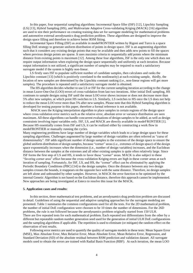
a. Test problem 1: 2D Shekel function

The Shekel function (Equation 1) is multimodal and can have any number of maxima [4]. In equation 1, N is

the number of dimensions. The number of maxima are defined by the row size of matrix a. “a” is a matrix of size M

rows by N columns. c is a vector of size M X 1. The matrix “a” contains the M number of positions of maxima

while the vector c defines the width of the maxima.

eq.1

Here, N=2, M=5, and , X1 and X2 are from [0, 1].

The 3D function plot of Shekel function is shown in Figure 2(a).

6

Figure 2. (a) 2D Shekel function plot; ISF, LIP, HYBRID and MACK strategies comparison on Shekel

function using error metric (b) Mean square error (c) Max absolute error (d) Max relative error (e)

Regression (f) Standard deviation.

Figures 2(b)-2(f) show the error metrics averaged from the 5 repeated tests for each. Each error metric clearly

shows that RSM created using sample generated by MACK outperforms the RSM created using samples generated

by other three methods. After 5 samples being added for 36 iterations, MACK has reached 3.98% of the Max

Relative Error and its Regression value is extremely close to 1, which is a sign of convergence. Among the ISF,

LS, and HS, not much difference is observed from all the charts except for the Max Absolute Error. ISF is slightly

outperformed by the LS and HS. Interestingly, LS is outperformed by the ISF and HS before iteration 11 on many

-0.1

999.9

1999.9

0 10 20 30 40

Me

an S

qu

are

Err

or

(me

an v

alu

e

fro

m 5

re

pe

ate

d t

est

s)

Iteration (b)

Shekel function: Mean Square Error Comparsion

mean_sq_error_ISF

mean_sq_error_LIP

mean_sq_error_HYBRID

mean_sq_error_MACK

0

100

200

300

400

500

0 10 20 30 40

Max

Ab

solu

te E

rro

r (m

ean

val

ue

fro

m

5 r

ep

eat

ed

te

sts)

Iteration (c)

Shekel function: Max Absolute Error Comparison

Max_abs_Err_ISF

Max_abs_Err_LIP

Max_abs_Err_HYBRID

Max_abs_Err_MACK

0

50

100

150

200

250

0 10 20 30 40Max

Re

lati

ve E

rro

r (m

ean

val

ue

fro

m 5

re

pe

ate

d t

est

s)

Iteration (d)

Shekel function: Max Relative Error comparsion

Max_re_Err_ISF

Max_re_Err_LIP

Max_re_Err_HYBRID

Max_re_Err_MACK

0

0.2

0.4

0.6

0.8

1

1.2

0 10 20 30 40

Re

gre

ssio

n (m

ean

val

ue

fro

m 5

re

pe

ate

d t

est

s)

Iteration (e)

Shekel function: Regression comparison

Regression_ISF

Regression_LIP

Regression_HYBRID

Regression_MACK

0

5

10

15

20

25

30

35

40

0 10 20 30 40

Stan

dar

d D

evi

atio

n (

me

an v

alu

e

fro

m 5

re

pe

ate

d t

est

s)

Iteration (f)

Shekel function: Standard Deviation Comparsion

stdev_ISF

stdev_LIP

stdev_HYBRID

stdev_MACK

2D Shekel function plot (a)

7

error metrics. This may imply that the LS is not as efficient on improving the surrogate modeling accuracy if the

number of initial samples is not sufficient to capture all the more non-linear regions in the design space.

b. Test problem 2: 2D h1 function

The h1function has a unique maximum value of 2.0 at the point (8.6998, 6.7665) [15]. In this study, the

bounds for the two design variables are [-20,20]. The function is described in Eq. 2 and the plot is shown in Figure

3(a).

eq. 2

Figures 3(b) – 3(f) illustrate the averaged error metrics obtained by comparing the RBF RSM prediction with

the 10000ULH validation dataset. Interestingly, MACK suddenly goes off scale at the iteration 27, and remains

unstable for the rest of the iterations. However, it does outperform the other three algorithms before iteration 17.

After close inspection of the design samples, it turns out that out of the 5 repeated tests, some of the trained RBF

surrogate models are ill-conditioned. The ill-conditioned surrogate models are not repeatable by training the same

dataset again using the Kriging algorithm. It is advised to try different parameter settings of RBF or RSM training

algorithms when abnormal behavior is observed. Therefore, we still conclude that for this test problem, MACK is

recommended due to its best performance among the four. From all the plots of error metrics, it indicates the errors

remain high after 36 iterations of sequential samplings; this is mostly due to that the h1 function is much more

difficult to fit than the Shekel function. Among the ISF, LS, and HS, they are again not much difference except for

the plots of Max Relative Error where HS outperforms ISF and LS starting from iteration 13.

0

0.01

0.02

0 10 20 30 40

Me

an S

qu

are

Err

or

(me

an v

alu

e

fro

m 5

re

pe

ate

d t

est

s)

Iteration (b)

h1 function: Mean Square Error Comparsion

mean_sq_error_ISFmean_sq_error_LIPmean_sq_error_HYBRIDmean_sq_error_MACK

0

0.2

0.4

0.6

0.8

1

1.2

1.4

1.6

0 10 20 30 40

Max

Ab

solu

te E

rro

r (m

ean

val

ue

fro

m 5

re

pe

ate

d t

est

s)

Iteration (c)

h1 function: Max Absolute Error Comparison

Max_abs_Err_ISFMax_abs_Err_LIPMax_abs_Err_HYBRIDMax_abs_Err_MACK 0

100000

200000

300000

400000

500000

600000

700000

0 10 20 30 40

Max

Re

lati

ve E

rro

r (m

ean

val

ue

fro

m 5

re

pe

ate

d t

est

s)

Iteration (d)

h1 function: Max Relative Error comparsion

Max_re_Err_ISFMax_re_Err_LIPMax_re_Err_HYBRIDMax_re_Err_MACK

2D h1 function plot (a)

8

Figure 3. (a) 2D h1 function plot; ISF, LIP, HYBRID and MACK strategies comparison using error metrics

(b) Mean square error (c) Max absolute error (d) Max relative error (e) Regression (f) Standard deviation.

Concerns of sampling size in sequential sampling approach

All the tests that have been done so far have five samples appended to existing samples at each iteration. One

question is will a different sampling size other than 5 at each iteration lead to different error decreasing rate? In this

section, the MACK and LS are compared on each 2D function. The ISF is not affected by the sampling size

because it always adds samples uniformly. Figures 4(a) – 4(d) compare the MSE associated with 5, 20, and 90

design samples at each iteration.

The figures illustrate that the different sampling size does not affect the performance of MACK. However, it

affects the performance of LS on both functions. Furthermore, while adding 5 samples at each iteration seems the

best among three options for the Shekel function, adding 90 samples at each iteration decreases the error the most

for the h1 function, although not significantly more than the other three algorithms do. A complete study of the

effect of sampling size on RSM error decrease is beyond the scope of this paper. However, it is recommended to

keep the sampling size relatively small because whenever the sequential sampling approach has to be terminated,

the RSM error decreasing history from using the small sampling size is more informative.

-1.4

-1.2

-1

-0.8

-0.6

-0.4

-0.2

0

0.2

0.4

0.6

0.8

0 10 20 30 40

Re

gre

ssio

n (m

ean

val

ue

fro

m 5

re

pe

ate

d

test

s)

Iteration (e)

h1 function: Regression comparison

Regression_ISFRegression_LIPRegression_HYBRIDRegression_MACK

0

0.01

0.02

0.03

0.04

0.05

0.06

0.07

0.08

0 10 20 30 40

Stan

dar

d D

evi

atio

n (

me

an v

alu

e f

rom

5

rep

eat

ed

te

sts)

Iteration (f)

h1 function: Standard Deviation Comparsion

stdev_ISFstdev_LIPstdev_HYBRIDstdev_MACK

0

500

1000

1500

2000

0 50 100 150 200

Me

an S

qu

are

Err

or

Number of points added by sequential sampling (a)

Shekel function - Lipschitz

Mean_sq_Err_5INCR_LIP

Mean_sq_Err_20INCR_LIP

Mean_sq_Err_90INCR_LIP

0

200

400

600

800

1000

1200

1400

1600

1800

0 50 100 150 200

Me

an S

qu

are

Err

or

Number of points added by sequential sampling (b)

Shekel function -MACK

Mean_sq_Err_5INCR_MACK

Mean_sq_Err_20INCR_MACK

Mean_sq_Err_90INCR_MACK

0

0.005

0.01

0.015

0 50 100 150 200

Me

an S

qu

are

Err

or

Number of points added by sequential sampling (c)

h1 function - Lipschitz

Mean_sq_Err_5INCR_LIPMean_sq_Err_20INCR_LIPMean_sq_Err_90INCR_LIP

0

0.005

0.01

0.015

0 50 100 150 200

Me

an S

qu

are

Err

or

Number of points added by sequential sampling (d)

h1 function - MACK

Mean_sq_Err_5INCR_MACKMean_sq_Err_20INCR_MACKMean_sq_Err_90INCR_MACK

9

Figure 4. Mean square error associated with 5,20 and 90 design samples at each iteration of (a)Shekel

function using Lipschitz (b) Shekel function using MACK (c)h1 function using Lipschitz (d) h1 function

using MACK algorithm.

c. Test problem 3: 5D Rosenbrock function

The Rosenbrock function [17] can be extended to any size of dimension, which is suitable for benchmarking

design optimization algorithms. This function is used here to test the four RSM sampling algorithms. Eq. 3

describes the function:

Eq 3

All design variables have same bounds: [-5, 10].

Figure 5(a)-(f) illustrate the changes of error values. Interestingly, the MACK is outperformed by all three other

sequential sampling algorithms. This is mainly due to the “boarder/corner” effect discussed in previous section.

Figure 6 shows a scatter matrix plot of the design samples added by the MACK. Those design samples are marked

in green color. It is obvious that large number of designs samples is added at the extremes of the design space

instead of contributing to the actual non-linear regions. Among the ISF, LS, and HS, ISF seems having the best

performance. This behavior could be due to the Rosenbrock function is essentially difficult to fit with any RSM

because the nature of its design space. Using any exploitation based algorithms such as LS or HS could be tricked

by the difficult nature of the function. Indicated from all charts of error metrics, ISF which uniformly explores the

design space is more efficient than the other three. It could imply that the solution space is noisy everywhere, and

the LS or HS may only concentrate at very limited number of identified non-linear regions, which is not efficient.

1.00E+04

1.00E+06

1.00E+08

1.00E+10

0 10 20 30 40

Me

an S

qu

are

Err

or

(me

an v

alu

e f

rom

5

rep

eat

ed

te

sts)

Iteration (a)

Mean Square Error Comparsion (y axis in logarithmic scale)

mean_sq_error_ISF

mean_sq_error_LIP

mean_sq_error_HYBRID

mean_sq_error_MACK

0.01

0.1

1

10

100

1000

0 10 20 30 40

Me

an R

ela

tive

Err

or

(me

an v

alu

e

fro

m 5

re

pe

ate

d t

est

s)

Iteration(b)

Mean Relative Error Comparison (y axis in logarithmic scale)

Mean_rel_Err_ISFMean_rel_Err_LIPMean_rel_Err_HYBRIDMean_rel_Err_MACK

1000

10000

100000

1000000

10000000

0 10 20 30 40

Max

Ab

solu

te E

rro

r (m

ean

val

ue

fro

m 5

re

pe

ate

d t

est

s)

Interation(c)

Max Absolute Error Comparison (y axis in logarithmic scale)

Max_abs_Err_ISFMax_abs_Err_LIPMax_abs_Err_HYBRIDMax_abs_Err_MACK

10

100

1000

10000

100000

0 10 20 30 40

Max

Re

lati

ve E

rro

r (m

ean

val

ue

fr

om

5 r

ep

eat

ed

te

sts)

Iteration(d)

Max Relative Error comparsion (y axis in logarithmic scale)

Max_re_Err_ISF Max_re_Err_LIP

Max_re_Err_HYBRID Max_re_Err_MACK

10

Figure 5. RSM error metrics comparison for 5D Rosenbrock function (a) Max Absolute error (b) Max

Relative error (c) Mean Absolute error (d) Mean Relative error (e) Regression (f) Standard deviation.

Figure 6. Border and corner effects in MACK

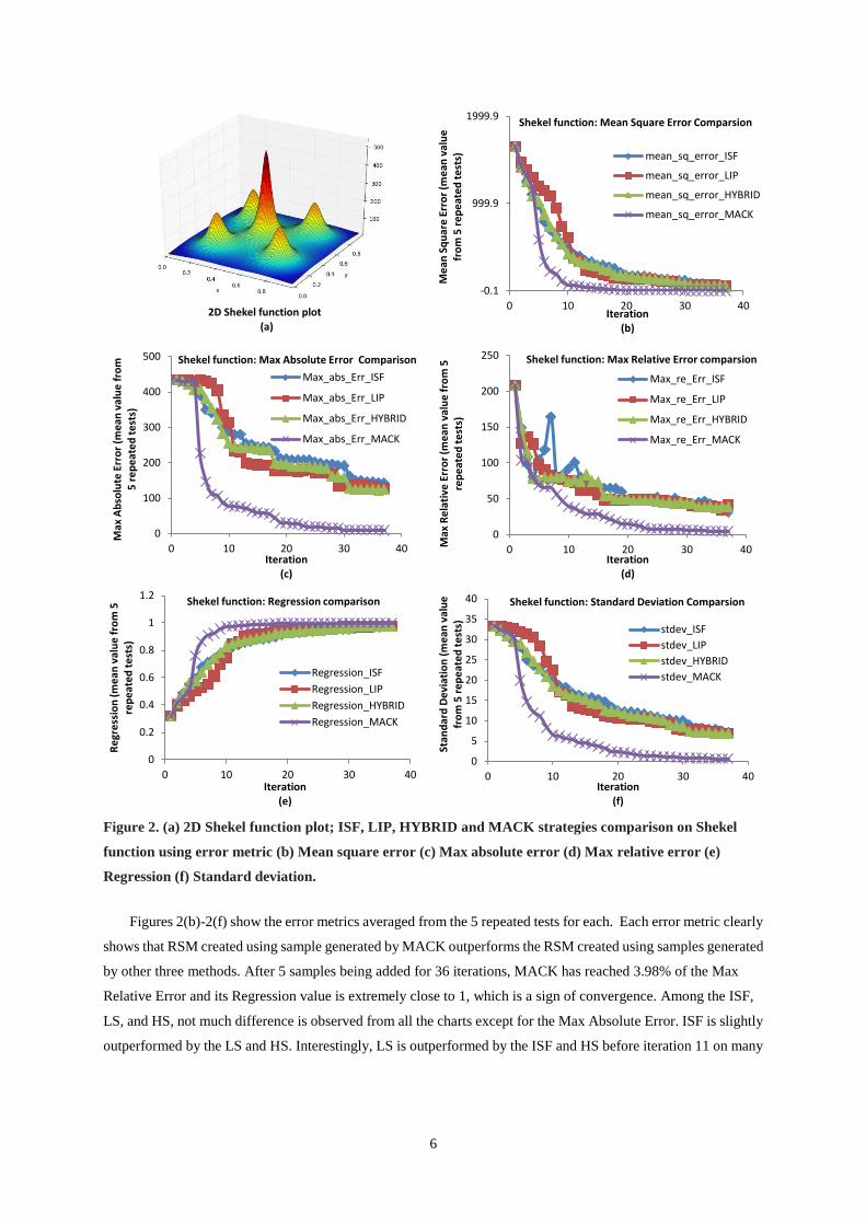
d. Test problem 4: 26D Rosenbrock function

In this test, number of design variable is 26. All have the bounds [-5,10]. MACK is not included in the test due

to the “border/corner” effect. Figure 7(a)-(f) illustrates the value of error metrics for each iteration. Among these

error metrics, only the maximum relative error plot indicates noticeable differences. Interestingly, the Max

absolute Error shows that the LS is the best in the last iterations but the Max Relative Error shows that the ISF is

the best for most of the later iterations. This may again indicate that the solution space may be quite noisy – simply

there are too many non-linear regions with equal strength. Algorithms such as LS or HS do not demonstrate

advantage, or large number of iterations of sequential sampling is required before they can show their strength.

0.80

0.85

0.90

0.95

1.00

1.05

0 10 20 30 40

Re

gre

ssio

n (m

ean

val

ue

fro

m 5

re

pe

ate

d

test

s)

Iteration(e)

Regression comparison

Regression_ISF Regression_LIP

Regression_HYBRID Regression_MACK

100

1000

10000

100000

1000000

0 10 20 30 40

Stan

dar

d D

evi

atio

n (

me

an v

alu

e f

rom

5

rep

eat

ed

te

sts)

Iteration(f)

Standard Deviation Comparsion (y axis in logarithmic scale)

stdev_ISF stdev_LIP

stdev_HYBRID stdev_MACK

11

Figure 7. RSM error metrics comparison for 26D Rosenbrock function (a) Max Absolute error (b) Max

Relative error (c) Mean Absolute error (d) Mean Relative error (e) Regression (f) Standard deviation.

e. Test problem 5: Aerodynamics drag prediction

In the automotive industry, although the use of Computational Fluid Dynamics (CFD) simulations for external

aerodynamics on a complete passenger car model has become common, the use of DoE and Optimization is not

common because of the computational cost involved. While CFD tools are becoming more accurate, they are also

computationally expensive. For a passenger car or light duty truck model, a full external aerodynamic CFD

simulation to calculate Coefficient of Drag (Cd) can take from a few hours to a couple of days using a HPC cluster

depending on mesh size and other simulation parameters. This complicates the use of optimization as well as real

time decision making during trade-off studies. Therefore, the goal is to develop a high fidelity RSM, which can

1.50E+11

1.70E+11

1.90E+11

2.10E+11

2.30E+11

2.50E+11

2.70E+11

2.90E+11

3.10E+11

0 10 20 30 40

Me

an S

qu

are

Err

or

(me

an v

alu

e f

rom

5

rep

eat

ed

te

sts)

Iteration (a)

mean_sq_error_ISFmean_sq_error_LIPmean_sq_error_HYBRID

10

11

12

13

14

15

16

0 10 20 30 40

Me

an R

ela

tive

Err

or

(me

an v

alu

e f

rom

5

rep

eat

ed

te

sts)

Iteration (b)

Mean_rel_Err_ISFMean_rel_Err_LIPMean_rel_Err_HYBRID

1800000

1900000

2000000

2100000

2200000

2300000

2400000

2500000

2600000

0 10 20 30 40

Max

Ab

solu

te E

rro

r (m

ean

val

ue

fro

m 5

re

pe

ate

d t

est

s)

Interation (c)

Max_abs_Err_ISF

Max_abs_Err_LIP

Max_abs_Err_HYBRID

100

120

140

160

180

200

220

0 10 20 30 40

Max

Re

lati

ve E

rro

r (m

ean

val

ue

fro

m

5 r

ep

eat

ed

te

sts)

Iteration (d)

Max_re_Err_ISF Max_re_Err_LIP Max_re_Err_HYBRID

0.720.740.760.78

0.80.820.840.860.88

0 10 20 30 40

Re

gre

ssio

n (m

ean

val

ue

fro

m 5

re

pe

ate

d t

est

s)

Iteration (e)

Regression_ISF

Regression_LIP

Regression_HYBRID

230000

250000

270000

290000

310000

330000

350000

0 10 20 30 40

Stan

dar

d D

evi

atio

n (

me

an v

alu

e

fro

m 5

re

pe

ate

d t

est

s)

Iteration (f)

stdev_ISF stdev_LIP stdev_HYBRID

12

accurately predict the Cd during the design negotiation, and eliminate the need of re-running the expensive CFD

simulations.

For the problem being considered in this work, there are total of 26 design variables. 25 of them are geometry

variables and continuous within their own physical bounds but one is a control/status variable which only has two

integer values: 0 and 1 to choose between two different shapes of a certain body section. The design variables also

have certain restrictions between each other defined by three constraints which are purely functions of design

variables. All the sampling algorithms discussed here can handle this kind of constraints and ensure the design

samples only go to simulations if they are feasible.

As indicated from Table 1, the sampling starts from 150 ULH DOE, then adding 32 design samples

concurrently by either ISF or LS, in separate tests. Please note that the MACK and HS is not included in this test,

because the MACK is subject to the “corner” and “border” when facing large dimensional problems, and the tests

with HS is current undergoing and not available yet. Also, for each sampling algorithm tested here, i.e., ISF or

Lipschitz, there is only one batch run of 32 design samples instead of 5 repetitions, simply because the CFD

simulations are expensive even they are evaluated concurrently. Lastly, among each batch run of 32 design

samples, there are always a few design samples for which the Cd value is unrealistic because the CFD calculation

did not converge. These invalid design samples are manually inspected and removed before they are included into

the next iteration of sequential sampling.

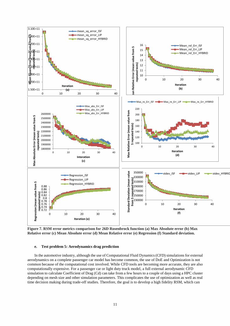
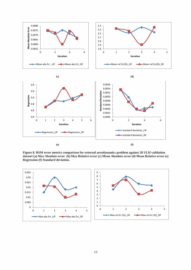
Figure 8(a)-(f) illustrates the error values between the 28 ULH validation dataset and the prediction from the

RSM. Although the ISF seems better before iteration 4, the LS outperforms the ISF at iteration 5 and 6. It’s more

obvious from the error values of Max absolute/relative errors. This confirms that the LS works because the LS has

found the non-linear regions and added samples there. Unlike the mathematical problem, it is not possible to

generate a validation dataset of 10000. Then how to accommodate any potential issue of using a relatively small as

well as static validation dataset? Here a so-called “moving” validation dataset is proposed. The idea is to use the

newly obtained design samples at each iteration as the validation dataset for the RSM trained from existing data up

to last iteration. In other words, the new design samples obtained from each iteration is used to validate the RSM

trained from last iteration. Therefore, the validation dataset is no longer static. This process of “generate batch of

new samples -> RSM training without the new samples -> validate the trained RSM” repeats until all the error

metrics converged or a satisfactory RSM is reached. Figure 9(a)–(f) shows the error values associated with the

“moving” validation datasets. It is interesting to see that the ISF outperforms the LS, which seems to be opposite to

the results in figure 8. This is because the error values are generated by comparing RSM trained without the new

samples and the new samples themselves – samples added by using LS are in the more non-linear regions

comparing to the samples generated by the ISF, which means it’s more difficult to predict these samples by the

RSM trained without the new samples.

Please note that the work of testing this problem is still undergoing. The authors are ready to test several

reduced dimensional problems 5D and 10D to compare their RSM error decreasing rates to this 26D problem.

(a)

(b)

0.0140.0150.0160.0170.0180.0190.0200.0210.022

0 2 4 6

Max

Ab

s Er

ror

Iteration

Max abs Err _LIP Max abs Err _ISF

4.0

4.5

5.0

5.5

6.0

6.5

0 2 4 6

Max

Re

lati

ve E

rro

r

Iteration

Max rel Err(%) _LIP Max rel Err (%)_ISF

13

(c)

(d)

(e)

(f)

Figure 8. RSM error metrics comparison for external aerodynamics problem against 28 ULH validation

dataset (a) Max Absolute error (b) Max Relative error (c) Mean Absolute error (d) Mean Relative error (e)

Regression (f) Standard deviation.

0.0055

0.0060

0.0065

0.0070

0.0075

0.0080

0 2 4 6

Me

an A

bso

lute

Err

or

Iteration

Mean abs Err _LIP Mean abs Err_ISF

1.8

1.9

2.0

2.1

2.2

2.3

2.4

0 1 2 3 4 5

Iteration

Mean rel Err(%)_LIP Mean rel Err(%)_ISF

0.8

0.8

0.8

0.9

0.9

0.9

0 1 2 3 4 5 6

Re

gre

ssio

n

Iteration

Regression_LIP Regression_ISF

0.0040

0.0042

0.0044

0.0046

0.0048

0.0050

0.0052

0.0054

0.0056

0 2 4 6

Stan

dar

d D

evi

atio

n

Iteration

standard deviation_LIP

standard deviation_ISF

0

0.005

0.01

0.015

0.02

0.025

0.03

0.035

0 1 2 3 4 5

Max abs Err_LIP Max abs Err_ISF

0

1

2

3

4

5

6

7

8

9

0 1 2 3 4 5

Max rel Err (%)_LIP Max rel Err (%)_ISF

14

Figure 9. RSM error metrics comparison for external aerodynamics problem against moving validation

dataset: (a) Max Absolute error (b) Max Relative error (c) Mean Absolute error (d) Mean Relative error (e)

Regression (f) Standard deviation.

8. Conclusion

Many CAE simulations require expensive computing resources and large amount of time. In vehicle industry,

this causes critical issues between the vehicle external aerodynamics engineers and design studio when vehicle

designs have to be negotiated and modified rapidly. Engineers are seeking high fidelity surrogate modeling of the

actual physical system to help them shorten the design process. This paper investigates four sequential sampling

algorithms: Incremental Space Filler (ISF), Lipschitz Sampling (LS), Hybrid Sampling, and Multivariate Adaptive

Crossvalidating Kriging (MACK) to see whether they can improve the RSM quality by a sequential sampling

fashion and how efficient they can be. Four mathematical problems and one Aerodynamics drag prediction

problem are tested extensively with these four algorithms. Based on the test results, it is concluded that: 1) the

decreasing of RSM error and number of design samples is not linearly correlated. Engineers often like to estimate

how many design samples they will need to plan ahead but this is difficult due to this reason; 2) For low

dimensional problems such as 1D or 2D, MACK is recommended as an sequential sampling algorithm; however, it

is not recommended to use MACK if the problem has more than two dimensions because the “border” or “corner”

effect; 3) For Lipschitz Sampling and Hybrid Sampling, when the total amount of design samples is fixed, different

sampling size may lead to different RSM error decreasing rate. However, small increment of design samples is

recommended simply because it provides more information of the sequential sampling history; 4) for high

dimensional problems with unknown complexity, Hybrid Sampling is recommended because it always shows

decent performance if not the best, which is observed from the test of difficult mathematical problems (2D h1, 5D

and 26D Rosenbrock function).

9. References

[1] modeFRONTIER® is a product of ESTECO spa (www.esteco.com)

[2] Jin, Ruichen, Wei Chen, and Agus Sudjianto. "On sequential sampling for global metamodeling in engineering

design." Proceedings of DETC. Vol. 2. 2002.

0

0.002

0.004

0.006

0.008

0 1 2 3 4 5

Mean abs Err_LIP Mean abs Err_ISF

0

0.5

1

1.5

2

2.5

0 1 2 3 4 5

Mean rel Err(%)_LIP Mean rel Err(%)_ISF

0.82

0.84

0.86

0.88

0.9

0.92

0.94

0.96

0 1 2 3 4 5

Regression_LIP Regression_ISF

0

0.001

0.002

0.003

0.004

0.005

0.006

0.007

0 1 2 3 4 5

standard deviation_LIP standard deviation_ISF

15

[3] Simpson, Timothy W., Dennis KJ Lin, and Wei Chen. "Sampling strategies for computer experiments: design

and analysis." International Journal of Reliability and Applications 2.3 (2001): 209-240.

[4] Crombecq, K., Gorissen, D., Deschrijver, D., & Dhaene, T. "A novel hybrid sequential design strategy for

global surrogate modeling of computer experiments." SIAM Journal on Scientific Computing 33.4 (2011):

1948-1974.

[5] dos Santos, M. Isabel Reis, and Pedro M. Reis dos Santos. "Sequential designs for simulation experiments:

Nonlinear regression metamodeling." Proceedings of the 26th IASTED International Conference on Modelling,

Identification, and Control. ACTA Press, 2007.

[6] Gramacy, Robert B., Herbert KH Lee, and William G. Macready. "Parameter space exploration with Gaussian

process trees." Proceedings of the twenty-first international conference on Machine learning. ACM, 2004.

[7] Cohn, David A. "Neural network exploration using optimal experiment design." (1994).Advances in Neural

Information Processing Systems, 1996, pp. 679–686. Morgan Kaufmann Publishers.

[8] MacKay, David JC. "Information-based objective functions for active data selection." Neural computation 4.4

(1992): 590-604.

[9] Maljovec, Dan, et al. "Adaptive Sampling with Topological Scores." Int. J. Uncertainty

Quantification,(accepted) (2012).

[10] Crombecq, Karel, and Tom Dhaene. "Generating sequential space-filling designs using genetic algorithms

and Monte Carlo methods." Simulated Evolution and Learning. Springer Berlin Heidelberg, 2010. 80-84.

[11] Provost, Foster, David Jensen, and Tim Oates. "Efficient progressive sampling." Proceedings of the fifth ACM

SIGKDD international conference on Knowledge discovery and data mining. ACM, 1999.

[12] Rigoni E., and Turco, A., “Metamodels for fast Multi-Objective Optimization: Trading Off Global

Exploration and Local Exploitation,” Proceedings of the SEAL 2010 LNCS 6457, pp.523-532, Kanpur, India,

2010.

[13] Lovison Alberto, and Rigoni Enrico, "Adaptive sampling with a Lipschitz criterion for accurate

metamodeling," Communications in Applied and Industrial Mathematics ISSN:2038-0909 Vol. 1, No. 2, 2010.

[14] Schlick T. Molecular Modeling and Simulation: An Interdisciplinary Guide. Interdisciplinary Applied

Mathematics series, Springer: New York, NY, USA. ISBN 0-387-95404-X, vol. 21,pp272-6, 2002

[15] Knoek van Soest, A. J. Knoek The Merits of a Parallel Genetic Algorithm in Solving Hard Optimization

Problems, J. Biomech. Eng. 125, 141.

[16] Turco, A., "MACK Implementation in modeFRONTIER 4.4," ESTECO Technical Report 2011-001, Trieste,

Italy, 2011.

[17] Rosenbrock, H. H., "An automatic method for finding the greatest or least value of a function", The Computer

Journal 3: 175–184, doi:10.1093/comjnl/3.3.175, ISSN 0010-4620, MR0136042, 1960.