rsm/cvs system user’s manual - fsu coapscoaps.fsu.edu/prediction/g-rsm/rsm_cvs_v2.1.pdf ·...

RSM/CVS System User’s Manual

Experimental Climate Prediction Center Scripps Institution of Oceanography, La Jolla, CA

(http://ecpc.ucsd.edu/projects/RSM/)

by

Hideki Kanamaru ([email protected]), Jongil Han, and Masao Kanamitsu

Version 2.1 - Updated on August 25th, 2004

http://ecpc.ucsd.edu/projects/RSM/

Contents

Contents...................................................................................................................................................... 2 1. Introduction ............................................................................................................................................ 3 2. Installation of CVS System and RSM .................................................................................................... 4

2.1 CVS System Installation................................................................................................................... 4 (1) Installation ................................................................................................................................... 4 (2) CVS commands ............................................................................................................................ 5

2.2 Installation of RSM/CVS system...................................................................................................... 6 3. Overview of Model System Structure .................................................................................................... 8 4. Running the Model ............................................................................................................................... 10

4.1 Test run using ‘rsm’ script.............................................................................................................. 10 4.2 Reading the output files.................................................................................................................. 12 4.3 choosing the model resolution ........................................................................................................ 13 4.4 Changing other model options........................................................................................................ 15 4.5 choosing the model domain ............................................................................................................ 17

1) Mercator projection .................................................................................................................. 18 2) polar stereographic projection .................................................................................................. 18

5. Understanding the Model Structure...................................................................................................... 19 5.1 RSM/CVS model code tree ............................................................................................................ 19 5.2 File name conventions .................................................................................................................... 20 5.3 ‘libs’ directory ................................................................................................................................ 20 5.4 ‘rsm’ directory ................................................................................................................................ 20 5.5 ‘runs’ directory ............................................................................................................................... 21

6. Model Integration Road Map ............................................................................................................... 22 6.1 Initialization.................................................................................................................................... 23 6.2 Time integration ............................................................................................................................. 24 6.3 Save output ..................................................................................................................................... 25

2

1. Introduction

• The Regional Spectral Model (RSM/CVS) at Experimental Climate Prediction Center in Scripps Institution of Oceanography has been developed to work within ECPC/SIO's GSM(Global Spectral Model)/CVS.

• The RSM/CVS system is managed by Concurrent Versions System (CVS) and

controlled by configure files and Makefile system. • The RSM/CVS system is an efficient, stable, state of the art atmospheric model

designed for regional climate research. • The RSM/CVS has the same structure as the GSM/CVS so that updates of model

physics in the GSM/CVS system can be directly incorporated. • The RSM/CVS currently works on IBM-SP, Origin, and Dec-Alpha, Linux, Sun,

Mac, Cray, NEC SX-6, NEC Earth Simulator as of July 2004 and is being tested on other platforms.

• The RSM/CVS has a parallel open-MP capabilty and the speedup is about 300% for 4

CPUs. • Users can always access the latest version of the model through the CVS system.

3

2. Installation of CVS System and RSM 2.1 CVS System Installation

Copy and update the code

Develop and update the code

Model Developers

UsersECPC/SIO Repository

(1) Installation

• First check whether you already have CVS on your system. Type ‘cvs –h’. • If you do not have CVS, get the source codes or binaries from the cvs home page:

https://www.cvshome.org

• On CVS site, go to ‘CVS downloads’, and go to ‘CCVS/archives’ for source codes and ‘CCVS/binaries’ for binaries, and install them by following the README file.

• Prior to CVS installation, the computer system should meet the following requirements:

C compiler is installed. Fortran 90 compiler is installed. There is adequate disk space.

• For example, to install the source codes of CVS:

1. gunzip cvs-1.11.16.tar.gz 2. tar xvf cvs-1.11.16.tar 3. cd cvs-1.11.16 4. ./configure --prefix=directory_to_install_cvs 5. make 6. make install

• Set environmental variable and add the cvs_executable_directory to your path.

For example, add the following line to the .cshrc file: set PATH=($path cvs_executable_directory) • Set environmental variable CVSROOT to the CVS server at ECPC/SIO.

4

https://www.cvshome.org/

setenv CVSROOT :pserver:[email protected]:/rokka1/kana/cvs-server-root/cpscvs

(2) CVS commands • login: Type ‘cvs login’ (only once), and just hit return at the password prompt

to login the CVS server as a username ‘anoncvs’ as specified in CVSROOT in .cshrc file. The access is read only.

Some useful CVS commands: • cvs co module_name: Copy the directories and files registered under

module_name. • cvs diff file_name: Show the difference between your file and the file in the

repository. • cvs status file_name: Show the status of the file_name. • cvs log file_name: Show the detailed log of the file_name.

5

2.2 Installation of RSM/CVS system

After installing the CVS system, go to the directory where you want to install RSM. The installer will create three directories: ‘libs’, ‘rsm’, and ‘runs’.

Make sure you add ‘.’ To your PATH in .cshrc file.

Go to the directory where you want to install the model.

Type ‘cvs co install’. This will download ‘install’ script from the CVS server at ECPC/SIO that you designated in your .cshrc file.

Type ‘./install’. Do not forget to put ‘./’ to make sure that the local script file ‘install’ is called. Type ‘./install -- help’ for various installer options.

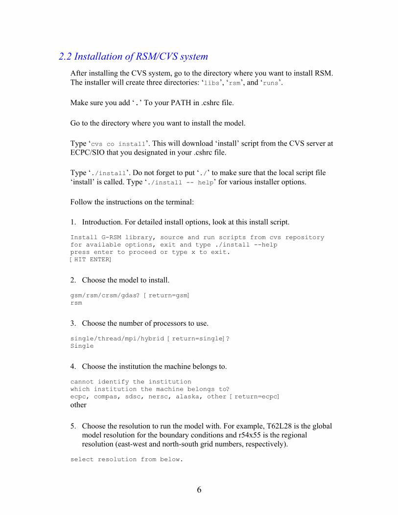
Follow the instructions on the terminal:

1. Introduction. For detailed install options, look at this install script. Install G-RSM library, source and run scripts from cvs repository for available options, exit and type ./install --help press enter to proceed or type x to exit. [HIT ENTER] 2. Choose the model to install. gsm/rsm/crsm/gdas? [return=gsm] rsm

3. Choose the number of processors to use. single/thread/mpi/hybrid [return=single]? Single

4. Choose the institution the machine belongs to. cannot identify the institution which institution the machine belongs to? ecpc, compas, sdsc, nersc, alaska, other [return=ecpc] other 5. Choose the resolution to run the model with. For example, T62L28 is the global

model resolution for the boundary conditions and r54x55 is the regional resolution (east-west and north-south grid numbers, respectively).

select resolution from below.

6

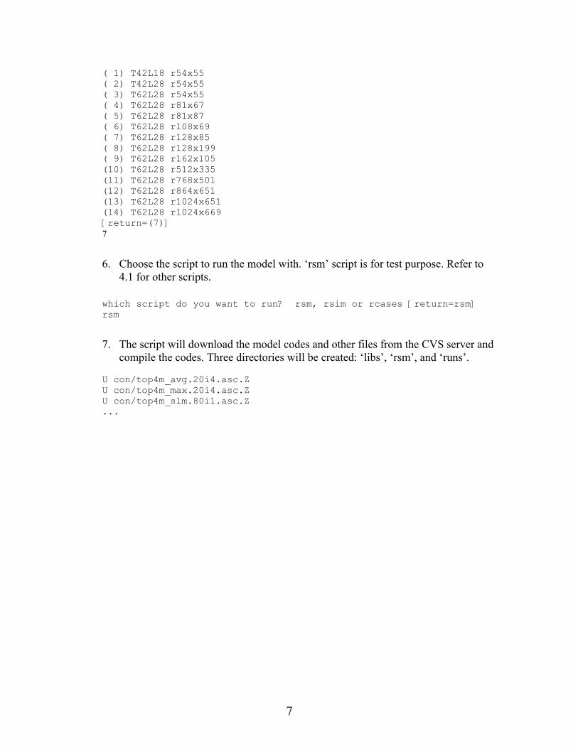
( 1) T42L18 r54x55 ( 2) T42L28 r54x55 ( 3) T62L28 r54x55 ( 4) T62L28 r81x67 ( 5) T62L28 r81x87 ( 6) T62L28 r108x69 ( 7) T62L28 r128x85 ( 8) T62L28 r128x199 ( 9) T62L28 r162x105 (10) T62L28 r512x335 (11) T62L28 r768x501 (12) T62L28 r864x651 (13) T62L28 r1024x651 (14) T62L28 r1024x669 [return=(7)] 7 6. Choose the script to run the model with. ‘rsm’ script is for test purpose. Refer to

4.1 for other scripts.

which script do you want to run? rsm, rsim or rcases [return=rsm] rsm

7. The script will download the model codes and other files from the CVS server and compile the codes. Three directories will be created: ‘libs’, ‘rsm’, and ‘runs’.

U con/top4m_avg.20i4.asc.Z U con/top4m_max.20i4.asc.Z U con/top4m_slm.80i1.asc.Z ...

7

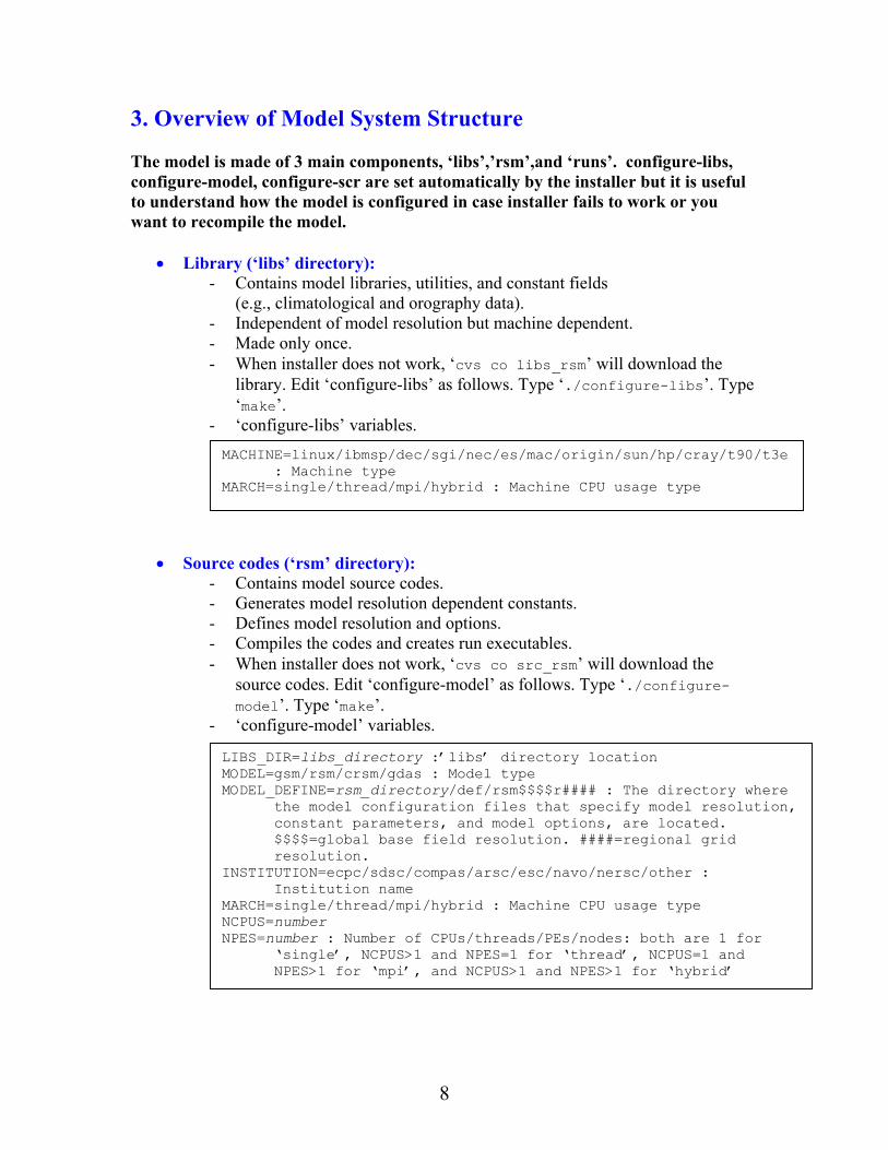
3. Overview of Model System Structure The model is made of 3 main components, ‘libs’,’rsm’,and ‘runs’. configure-libs, configure-model, configure-scr are set automatically by the installer but it is useful to understand how the model is configured in case installer fails to work or you want to recompile the model.

• Library (‘libs’ directory): - Contains model libraries, utilities, and constant fields

(e.g., climatological and orography data). - Independent of model resolution but machine dependent. - Made only once. - When installer does not work, ‘cvs co libs_rsm’ will download the

library. Edit ‘configure-libs’ as follows. Type ‘./configure-libs’. Type ‘make’.

- ‘configure-libs’ variables.

MACHINE=linux/ibmsp/dec/sgi/nec/es/mac/origin/sun/hp/cray/t90/t3e

: Machine type MARCH=single/thread/mpi/hybrid : Machine CPU usage type

• Source codes (‘rsm’ directory): - Contains model source codes. - Generates model resolution dependent constants. - Defines model resolution and options. - Compiles the codes and creates run executables. - When installer does not work, ‘cvs co src_rsm’ will download the

source codes. Edit ‘configure-model’ as follows. Type ‘./configure-model’. Type ‘make’.

- ‘configure-model’ variables. LIBS_MODELMODEL

INSTI

MARCHNCPUSNPES=

DIR=libs_directory :’libs’ directory location =gsm/rsm/crsm/gdas : Model type _DEFINE=rsm_directory/def/rsm$$$$r#### : The directory where the model configuration files that specify model resolution, constant parameters, and model options, are located. $$$$=global base field resolution. ####=regional grid resolution. TUTION=ecpc/sdsc/compas/arsc/esc/navo/nersc/other : Institution name =single/thread/mpi/hybrid : Machine CPU usage type =number number : Number of CPUs/threads/PEs/nodes: both are 1 for ‘single’, NCPUS>1 and NPES=1 for ‘thread’, NCPUS=1 and NPES>1 for ‘mpi’, and NCPUS>1 and NPES>1 for ‘hybrid’

8

• Run scripts (‘runs’ directory):

- Runs the model and stores the model outputs. - When installer does not work, , ‘cvs co scr_rsm’ will download the run

scripts. Edit ‘configure-scr’ as follows. See the next section for the next steps.

- ‘configure-scr’ variables.

SRCS_DIR=rsm_directory : ‘rsm’ directory location INSTITUTION= ecpc/sdsc/compas/arsc/esc/navo/nersc/other :

Institution name. Batch script templates are available in ‘runscr’ directory for some of the listed institutions.

NCPU_PER_NODE=number : Number of CPUs per node for mpi run

9

4. Running the Model 4.1 Test run using ‘rsm’ script Move to ‘runs’ directory. The installer created ‘rsm’ script in the directory from ‘expscr/rsm.in’ file as a template. If you want to make changes to the main ‘rsm’ run script, you can either edit the ‘rsm’ script directly or edit the template ‘expscr/rsm.in’ and ‘configure-scr rsm’. ‘configure-scr’ takes script_name as an argument and creates main run scripts from the specified template. The main run script template has to be in ‘expscr’ directory as ‘script_name.in’. There are several run script templates available.

• ‘rsim’: Performs rsm long integrations forced by global analysis or forecasts. Various options are available for monthly average calculations and archives.

• ‘rcases’: Performs many short rsm integrations forced by short global forecasts. • ‘rsm’: Performs test run (explained below).

‘configure-scr’ also creates other scripts in ‘runscr’ directory from their templates . The scripts in ‘runscr’ directory are called by the main run scripts.

For the test purpose, we use ‘rsm’ script. The ‘rsm’ script runs from 1990 March 9th 00 hours for 48 hours. The initial and boundary conditions are pre-made and stored in ‘libs/con’ directory. The key parameters are explained below.

10

RUNNAME=r_000 : The name of the directory where the output files are created.]

rsm domain specifications [see also 4.5] RPROJ=1. RTRUTH=60. RORIENT=-100. RDELX=60000. : The model resolution in x direction in meters. RDELY=60000. : The model resolution in y direction in meters. RCENLAT=90. RCENLON=0. RLFTGRD=49. RBTMGRD=134. model parameters ENDHOUR=48 : End of the forecast integration in hours. DELTAT_REG=360 : The model time step in seconds. It should be

roughly proportional to the model resolution that is set above in RDELX and RDELY.

INTOUT=3 :The model output files (r_sig, r_flx, r_sfc, and r_pgb) interval in hours. Passed to INTSIG later in the script.

NESTING_HOUR=6: The nesting interval from the global file in hours.

SWHR_REG=1 : The shortwave radiation computation interval for regional model. Usually 1 hour.

LWHR_REG=1 : The longwave radiation computation interval for regional model. Usually 1 hour.

INTSFCX=24 : Grib surface files merging interval. It should be equal to or greater than 24 hours.

INCHOUR=12 : Forecast hour per one execution of the main forecast program rfcst.x.

11

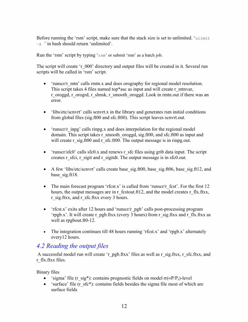
Before running the ‘rsm’ script, make sure that the stack size is set to unlimited. ‘ulimit –s ’ in bash should return ‘unlimited’. Run the ‘rsm’ script by typing ‘rsm’ or submit ‘rsm’ as a batch job. The script will create ‘r_000’ directory and output files will be created in it. Several run scripts will be called in ‘rsm’ script.

• ‘runscr/r_mtn’ calls rmtn.x and does orography for regional model resolution. This script takes 4 files named top*asc as input and will create r_mtnvar, r_oroggd, r_orogrd, r_slmsk, r_smooth_oroggd. Look in rmtn.out if there was an error.

• ‘libs/etc/scnvrt’ calls scnvrt.x in the library and generates rsm initial conditions

from global files (sig.ft00 and sfc.ft00). This script leaves scnvrt.out.

• ‘runscr/r_inpg’ calls rinpg.x and does interpolation for the regional model domain. This script takes r_smooth_oroggd, sig.ft00, and sfc.ft00 as input and will create r_sig.ft00 and r_sfc.ft00. The output message is in rinpg.out.

• ‘runscr/sfc0’ calls sfc0.x and renews r_sfc files using grib data input. The script

creates r_sfci, r_sigit and r_sigitdt. The output message is in sfc0.out. • A few ‘libs/etc/scnvrt’ calls create base_sig.ft00, base_sig.ft06, base_sig.ft12, and

base_sig.ft18. • The main forecast program ‘rfcst.x’ is called from ‘runscr/r_fcst’. For the first 12

hours, the output messages are in r_fcstout.ft12, and the model creates r_flx.ftxx, r_sig.ftxx, and r_sfc.ftxx every 3 hours.

• ‘rfcst.x’ exits after 12 hours and ‘runscr/r_pgb’ calls post-processing program

‘rpgb.x’. It will create r_pgb.ftxx (every 3 hours) from r_sig.ftxx and r_flx.ftxx as well as rpgbout.ft0-12.

• The integration continues till 48 hours running ‘rfcst.x’ and ‘rpgb.x’ alternately

every12 hours.

4.2 Reading the output files A successful model run will create ‘r_pgb.ftxx’ files as well as r_sig.ftxx, r_sfc.ftxx, and r_flx.ftxx files. Binary files

• ‘sigma’ file (r_sig*): contains prognostic fields on model σ(≡P/Ps)-level • ‘surface’ file (r_sfc*): contains fields besides the sigma file most of which are

surface fields

12

• ‘flux’ file (r_flx*): contains diagnostic fields GRIB format files

• post-processed file (r_pgb*): GRIB files on pressure surface created from the sigma and flux binary files

GRIB format files such as ‘r_pgb.ftxx’ can be easily read and displayed with the software ‘GrADS’.

• Install GrADS graphic package from http://grads.iges.org/grads/ • Set path to ‘libs/etc/’ in .cshrc. • Type ‘grmap –g0 r_pgb.ftxx ’, which generates GrADS control file (*.ctl). • For example, ‘grmap r_pgb.ft03’ will create two control files

‘r_pgb.ft03.r_pdlr.ctl’ and ‘r_pgb.ft03.r_pprs.ctl’, and corresponding index files ‘r_pgb.ft03.r_pdlr.idx’ and ‘r_pgb.ft03.r_pprs.idx’. pdlr files are for soil moisture and temperature. ‘pprs’ fiels are for all other variables.

• If necessary, edit control files. To recreate index files, type ‘gribmap –i

control_file_name ’. • Start GrADS by typing ‘grads ’. • In GrADS, type ‘open control_file_name ’

• Type ‘q file 1’ to see what variables are available.

• Plot model output fields by typing ‘d variable_name ’

4.3 choosing the model resolution If you wan to change the model resolution, you need to recompile the source codes in ‘rsm’ directory. It is not necessary to recompile the libraries in ‘libs’ directory. Go to ‘rsm/def’ directory. Look for the model resolution you want to run. If you cannot find the desired resolution, users can always create a new directory for the resolution.

• Copy the directory whose resolution is similar to your desired resolution, and name it appropriately.

• Each directory has three files: define.h, modlsigs.h, and postplevs.h. • You will only need to edit define.h.

13

http://grads.iges.org/grads/

• igrd should be a product of integer powers of 2, 3, and 5. On IBM, integer power for 3 cannot be more than 2.

• jgrd should be an odd number. define.h (model resolution and other parameters)

jcap 62 : global truncated wave number levs 28 : number of global vertical sigma levels lonf 192 : number of global E-W Gaussian grids latg 94 : number of global N-S Gaussian grids (relationship between jcap and lonf and latg: lonf ≥ 3*jcap+1,latg ≥ (3*jcap+1)/2) lsoil 2 : number of soil layers lalbd 4 : number of albedo types mtnres 8 : topography resolution in minute (8min~15km) ncldg 0 : number of prognostic cloud species (cloud water/ice, rain/snow) nstype 9 : number of soil types nvtype 13 : number of vegetation types igrd 96 : number of regional x-axis grids (should be a product of integer powers of 2,3,5) jgrd 69 : number of regional y-axis grids (should be an odd number) levr 28 : number of regional vertical sigma levels cigrd1 192: number of coarse regional x-axis grids cjgrd1 94 : number of coarse regional y-axis grids relx 5 : lateral boundary relaxation parameter in terms of number of time steps (relx*∆t = 1800-3000 sec recommended, larger number implies less relaxation) border 3 : interpolation order (3: cubic) bgf 3 : interpolation parameter (bgf*dx is a size of user-

defined base grid [so called B-grid], to which the original driving base field is interpolated)

difuh 3 : numerical diffusion parameter for temperature and moisture in terms of number of time steps (larger number implies less diffusion) difum 2 : numerical diffusion parameter for momentum in terms of number of time steps (larger number implies less diffusion) ilonf 192 : number of E-W Gaussian grids in global input data ilatg 94 : number of E-W Gaussian grids in global input data ijcap 62 : truncated wave number in global input data ilevs 28 : number of vertical sigma levels in global input data

Go back to ‘rsm’ directory and edit ‘configure-model’ to set ‘MODEL_DEFINE’ to the directory of your resolution. The following steps are common procedure for recompiling the entire ‘rsm’ directory after changing variables in ‘configure-model’ or compiler options in ‘rsm/opt’ directory. ‘make clean ’ will delete all the files that the previous compilation created.

14

Type ‘configure-model’ to recreate new Makefiles and ‘define.h’, ‘machine.h’, ‘modlsigs.h’, and ‘postplevs.h’. Type ‘make to recompile the source codes and create new executables.

4.4 Changing other model options You can change model parameters and recompile the entire ‘rsm’ directory.

• Type ‘make clean ’. • Type ‘configure-model ’. • If you want to save the default settings, do not edit define.h in

‘rsm/def/rsm$$$$r####’. • Instead edit ‘define.h’ in ‘rsm’ directory. • All the model options are set using ‘#define’ and ‘#undef’. • Type ‘configure-model ’ again • Choose ‘configure with modified define.h’. • Type ‘make ’.

Some model options in define.h

#define NEWSFC : if defined, use new surface physics #undef NEWGWD : if defined, use new gravity wave drag formulation #undef CLDADJ : if defined, conduct cloud adjustment #define SAS : if defined, simplified Arakawa-Schubert cumulus cloud scheme #undef RAS : if defined, relaxed Arakawa-Schubert cumulus cloud scheme #if (_ncldg_==0) #undef ICE #undef ICECLOUD #else : for consideration of the effect of ice #define ICE and ice cloud on radiation #define ICECLOUD #endif #undef NEWALB #ifdef NEWSFC : if NEWSFC is defined, #define NEWALB use new albedo types #endif #define G2R : if defined, nesting from global to regional grid #undef C2R : if defined, nesting from coarse to fine regional grid

15

Land surface schemes (rsm/def/physics.h) • OSU (Oregon State University land surface scheme)

OSU1: the old version of OSU and used in NCAR/NCEP Reanalysis study OSU2: the new version of OSU and the land surface vegetation and soil type properties obtained from grib files OSU2 is available on RSM/CVS (#define OSULSM2 in physics.h).

• NOAH (NOAH land surface model) Developed in NCEP, OSU, Air force, Hydrologic Research Lab NOA1: maximum one-vegetation type considered in each cell NOA1 is available on RSM/CVS (#define NOALSM1 in physics.h).

• VIC (Variable Infiltration Capacity) Developed in the University of Washington, Seattle, and Princeton University VIC1: maximum one-vegetation type considered in each cell VIC1 will be available on RSM/CVS soon.

• CLM (Common Land Model) Developed in NCAR, NASA, GIT, and Beijing Normal UniversityüCombined the best features, as possible, of NCAR LSM (Bonan 1996), BATS (Dickinson 1993), and IAP94 (Dai and Zeng 1997) CLM will be available on RSM/CVS soon.

16

4.5 choosing the model domain If you want to change the model domain, you need to edit the main run script or its template in ‘runs/expscr’. Mapping and domain parameters in the main run script

RPROJ mapping projection index 0 for Mercater projection (MP) 1 for north polar stereographic projection (NPSP) -1 for south polar stereographic projection (SPSP) RTRUTH latitude where the map plane cuts through the earth’s surface A north latitude for MP 60o for NPSP -60o for SPSP RORIENT domain orientation longitude RDELX grid spacing in meter in x-direction at TRUTH. RDELY grid spacing in meter in y-direction at TRUTH. RCENLAT reference latitude domain center latitude for MP 90o for NPSP -90o for SPSP RCENLON reference longitude domain center longitude for MP 0 for both NPSP and SPSP RLFTGRD a grid number in x-direction RBTMGRD a grid number in y-direction

After setting the parameters in ‘expscr/script_name.in ’. Type ‘configure-scr script_name ’ to recreate the main run script. A utility ‘prmap’ in ‘lib/etc’ is useful for checking the domain definition.

• ‘prmap script_name ’ takes the model resolution from ‘rsm/define.h’ and model domain parameters from the main run script ‘script_name’ and create ‘prmap.ctl’ and ‘prmap.data’.

• Open ‘prmap.ctl’ in GrADS and plot the domain.

17

1) Mercator projection

LyLx

(RCENLON,RCENLAT)

RLFTGRD = INT(Lx/RDELX) RBTMGRD = INT(Ly/RDELY) 2) polar stereographic projection

pole

Ly

RLFTGRD = INT(Lx/RBTMGRD = INT(Ly/

Lx

RORIENT

RDELX) RDELY)

18

5.2 File name conventions Source and library related files:

• *.F: source codes with C-processor directives • *.f: source codes after C-processing • *.o: object codes • *.x: executables • *.a: libraries • *.h: includes • *.in: file templates • No suffix: makefile, scripts, or constants • *.sh : scripts • *.* files are created after compilation

Data and constant files:

• *.Z : compressed • *.asc : ascii file • *.grib : grib format file • *.ieee : ieee binary (single precision) file

Source code naming and format:

• One subroutine per file. File name is the same as the subroutine name. • Lower case for Fortran variables. • Upper case for C-processor variables • Use variables ending with ‘_ ‘ for parameter. • The definitions of the parameter variables appear in the include file,

‘paramodel.h’.

5.3 ‘libs’ directory

• configure-libs: library compilation configuration script. • Makefile: library make file. • ‘makefiles’ directory: ‘Makefile’ templates for creating libraries and constants. • ‘con’ directory: contains constants and climatology files. • ‘etc’ directory: contains miscellaneous utility files. • ‘lib’ directory: contains library source codes. • ‘opt_libs’ directory: contains compilation options for various machine types. • ‘make’ command generates the following.

1. grib packing and unpacking library (w3lib.a) 2. model utility library (modelib.a) 3. ncar utility library (ncaru.a) 4. executables for various utilities (*.x in etc directory) 5. scripts to run the executables (files without suffix in etc directory)

5.4 ‘rsm’ directory

20

• configure-model: source code compilation configuration script. • Makefile: make file for executables. • ‘makefiles’ directory: ‘Makefile’ templates for creating executables. • ‘def’ directory: defines parameters and constants depending on model resolution,

model options, and machine types. ‘function.h’ defines machine dependent statements. There are directories with varying model resolutions that specify model options and resolution dependent parameters and constants.

• ‘opt’ directory: contains files that specify compiler options for various machine types.

• ‘src’ directory: contains model source codes. • ’bin’ directory: contains model executables. The ‘bin’ directory is generated after

compilation of the codes. • ‘cvs_docs’ directory: contains help files. • ‘make ’ command creates libraries and executables. The libraries are generated

first and executables are made last, since it links libraries. In addition, ‘co2’ program are executed. ‘co2’ program interpolates co2 profile in vertical to the model levels.

• Occasionally, compilation fails due to various reasons. On some machines, even when there is an error in compilation ‘make’ does not fail and keeps running to the end. This results in missing executables when the program is executed. When this occurs, you need to go to the directory that the compilation failed and type ‘make’ to see why the compilation failed. Fix the error and type ‘make’ to complete the compilation for the program.

5.5 ‘runs’ directory

• configure-scr: run scripts configuration script. • ‘expscr’ directory: contain templates for main run scripts. • ‘runscr’ directory: contains various run scripts called by the main run scripts. • ‘cvs_docs’ directory: contains help files.

21

6. Model Integration Road Map (‘rsm/src’ directory has source codes)

rsmonly (rfcst): driving routine

Blue: directory

Green: subroutine

Initialization • rgetcon (rfcst) • rsmini (rsml) • tread (rgsm)

Time integration • rsmsmf (rsml)

Increment hour (e.g., 6 hours) of global boundary forcing

Save output • rsmsav (rsml)

22

6.1 Initialization

rgetcon (rfcst): • set model integration constants • set table for model physics

•

rsmini (rsml): • set more constants beyond rgetcon • rsminp (rsml) - read global base field

- gsm2bgd (rsml): transform spectral global input field to regional grid - sread (rsml): read regional sigma field to obtain regional perturbation in wave coefficients

• rfixio (rsml): read regional surface fields

tread (rgsm): read next global base field

23

6.2 Time integration

rsmsmf (rmsl): main routine

rsmltb (rmsl): compute base field tendency

rloopr (rmsl): compute radiation fluxes

rloopa (rmsl): compute total tendency tendency

rsicdif (rmsl): semi-implicit integration

rlatbnd (rmsl): update base field and its tendency

rloopd (rmsl): local wind speed damping

rupdate (rmsl): update perturbation

rdeldif (rmsl): horizontal diffusion

rfilt1 (rmsl): time filter step 1

rloopb (rmsl): model physics computation

rfilt2 (rmsl): time filter step 2

Increment of model time step (e.g., dt=360 sec)

Intermediate outputs (INTSIG)Surface merge (INTSFCX) Post-processing (INTSIG)

24

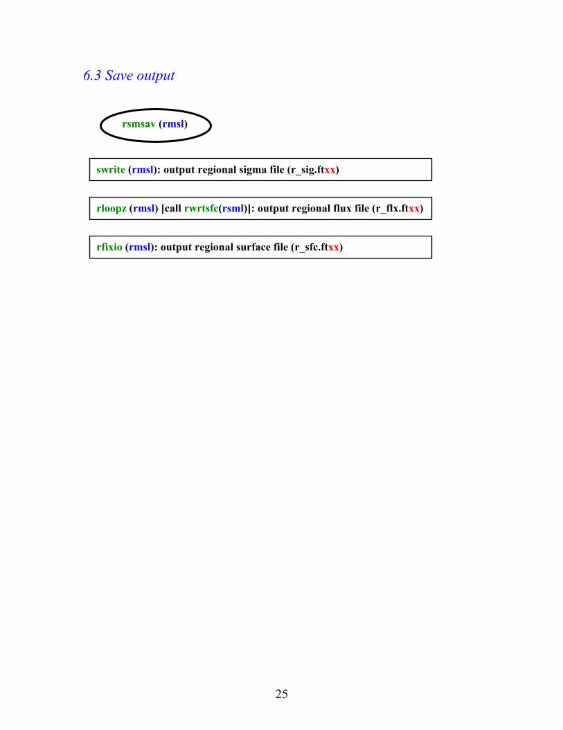
6.3 Save output

rsmsav (rmsl)

swrite (rmsl): output regional sigma file (r_sig.ftxx)

25

rloopz (rmsl) [call rwrtsfc(rsml)]: output regional flux file (r_flx.ftxx)

rfixio (rmsl): output regional surface file (r_sfc.ftxx)

rsm/cvs system user’s manual - fsu coapscoaps.fsu.edu/prediction/g-rsm/rsm_cvs_v2.1.pdf ·...

Documents