ruben manvelyan, karapet mkrtchyan and werner ruhl-general trilinear interaction for arbitrary even...

8/3/2019 Ruben Manvelyan, Karapet Mkrtchyan and Werner Ruhl-General trilinear interaction for arbitrary even higher spin g…

http://slidepdf.com/reader/full/ruben-manvelyan-karapet-mkrtchyan-and-werner-ruhl-general-trilinear-interaction 1/22

a r X i v : 1 0 0 3

. 2 8 7 7 v 1 [ h e p - t h ]

1 5 M a r 2 0 1 0

hep-th/ March 2010

General trilinear interaction for arbitrary evenhigher spin gauge fields

Ruben Manvelyan †‡, Karapet Mkrtchyan†‡

and Werner Ruhl †

†Department of Physics

Erwin Schr¨ odinger Straße

Technical University of Kaiserslautern, Postfach 3049

67653 Kaiserslautern, Germany

‡Yerevan Physics Institute

Alikhanian Br. Str. 2, 0036 Yerevan, Armenia

manvel,[email protected]; [email protected]

Abstract

Using Noether’s procedure we present a complete solution for the trilinear inter-actions of arbitrary spins s1, s2, s3 in a flat background, and discuss the possibilityto enlarge this construction to higher order interactions in the gauge field. Someclassification theorems of the cubic (self)interaction with different numbers of derivatives and depending on relations between the spins are presented. Finallythe expansion of a general spin s gauge transformation into powers of the fieldand the related closure of the gauge algebra in the general case are discussed.

http://arxiv.org/abs/1003.2877v1





































1 Introduction and notations

The motivation for the investigation of higher spin gauge field (HSF) interac-tions can be summarized as the following list of the essential three points:

1. The construction of interacting higher spin theories has been consideredas an interesting task for itself and was always in the center of attentionduring the last thirty years [1]-[17].

2. Particular attention arose during the last decade after discovering the holo-graphic duality between the O(N ) sigma model in d = 3 space and HSFgauge theory living in the space AdS 4 [18]. This case of holography is espe-cially important by the existence of two conformal points of the boundarytheory and the possibility to describe them by the same HSF gauge theory

with the help of spontaneous breaking of higher spin gauge symmetry and mass generation by a corresponding Higgs mechanism [21]-[23].

3. Another still open point is verifying the holographic correspondence on thelevel of loop diagrams in the general case, and the possibility to use thiscorrespondence for real constructions of unknown local interacting theorieson the bulk from more or less well known conformal field theories on theboundary.

These complicated physical tasks necessitate quantum loop calculations for theHSF field theory [24], [25],[26] and therefore information about the manifest, off-

shell and Lagrangian formulation of possible interactions for HSF. On the otherhand one loop calculations are mainly interesting in the framework of their ultra-violet behaviour, when the difference between an AdS and a flat space backgroundcan be neglected at least in the leading order. These motivations caused us duringlast years to spend some effort on the construction of possible couplings which westarted in series of articles that involved couplings among different higher spinfields [2, 3, 4, 19] . In our previous article [1] we directly construct a complete cu-bic selfinteraction for the case of spin s = 4 in a flat background, and discuss thecubic selfinteraction for general spin s with s derivatives in the same background.The leading term of the latter interaction together with the gauge transformationof first order in the field was presented and investigated.

Here we turn to the trilinear interaction of Fronsdal’s [20] general spin s1, s2, s3gauge fields in a flat background (Section 2) and present the full solution of the corresponding Noether’s equation (Section 3). Then we discuss a generalclassification theorem for (self)interactions based on our construction and therelation with other known couplings involving (Weyl) tensors integrated into theinteraction Lagrangians (Section 4). The last section 5 is devoted to a discussionof gauge transformations that are nonlinear in the gauge field, as they wereinvented in the classical paper [7], and the possibility to form Lie algebras of

2



gauge transformations for even spin abelian gauge fields and in this context theconstruction of the fourth and higher order selfinteractions.

To handle these sections we should introduce here briefly our standard nota-tions coming from our previous papers about HSF [1, 2, 3, 4, 19]. As usual we

utilize instead of symmetric tensors such as h(s)µ1µ2...µs(z) the homogeneous poly-

nomials in the vector aµ of degree s at the base point z

h(s)(z; a) =µi

(s

i=1

aµi)h(s)µ1µ2...µs

(z). (1.1)

Then we can write the symmetrized gradient, trace and divergence ∗

Grad : h(s)(z; a) ⇒ Gradh(s+1)(z; a) = (a∇)h(s)(z; a), (1.2)

T r : h(s)(z; a) ⇒ T rh(s−2)(z; a) = 1s(s − 1)

2ah(s)(z; a), (1.3)

Div : h(s)(z; a) ⇒ Divh(s−1)(z; a) =1

s(∇∂ a)h(s)(z; a). (1.4)

Moreover we introduce the notation ∗a, ∗b, . . . for a contraction in the symmetricspaces of indices a or b

∗a =1

(s!)2

si=1

←−∂ µi

a

−→∂ aµi

. (1.5)

Then we see that the operators (a∂ b), a2, b2 are dual (or adjoint) to (b∂ a),2a,2b

with respect to the ”star” product of tensors with two sets of symmetrized indices(1.5)

1

n(a∂ b)f (m−1,n)(a, b) ∗a,b g(m,n−1)(a, b) = f (m−1,n)(a, b) ∗a,b

1

m(b∂ a)g(m,n−1)(a, b), (1.6)

a2f (m−2,n)(a, b) ∗a,b g(m,n)(a, b) = f (m−2,n)(a, b) ∗a,b1

m(m − 1)2ag(m,n)(a, b). (1.7)

In the same fashion gradients and divergences are dual with respect to the fullscalar product in the space (z,a,b)

(a∇)f (m−1,n)(z; a, b) ∗a,b g(m,n)(z; a, b) = −f (m−1,n)(z; a, b) ∗a,b1

m(∇∂ a)g(m,n)(z; a, b).

(1.8)

Analogous equations can be formulated for the operators b2 or b∇.

∗To distinguish easily between ”a” and ”z” spaces we introduce the notation ∇µ for space-time derivatives ∂

∂zµ.

3



Here we will only present Fronsdal’s Lagrangian in terms of these conventions†:

L0(h(s)

(a)) = −

1

2h(s)

(a) ∗a F (s)

(a) +

1

8s(s − 1)2

ah(s)

(a) ∗a2

aF (s)

(a), (1.9)

where F (s)(z; a) is the Fronsdal tensor

F (s)(z; a) = 2h(s)(z; a) − s(a∇)D(s−1)(z; a), (1.10)

and D(s−1)(z; a) is the deDonder tensor or traceless divergence of the higher spingauge field

D(s−1)(z; a) = Divh(s−1)(z; a) −s− 1

2(a∇)T rh(s−2)(z; a), (1.11)

2aD(s−1)

(z; a) = 0. (1.12)

The initial gauge variation of order zeroth in the spin s field is

δ(0)h(s)(z; a) = s(a∇)ǫ(s−1)(z; a), (1.13)

with the traceless gauge parameter for the double traceless gauge field

2aǫ(s−1)(z; a) = 0, (1.14)

22ah(s)(z; a) = 0. (1.15)

Therefore at this point we can see from (1.13) and (1.14) that the de Dondergauge conditionD(s−1)(z; a) = 0, (1.16)

is a correct generalization of the Lorentz gauge condition in the case of spin s > 2.Finally we note that in deDonder gauge (1.16) F (s)(z; a) = 2h(s)(z; a) and thefield h(s) decouples from it’s trace in Fronsdal’s Lagrangian (1.9).

2 Noether’s theorem in leading order: Trino-

mial coefficients

We consider three potentials h(s1)(z1; a), h(s2)(z2; b), h(s3)(z3; c) whose spins si areassumed to be ordered

s1 ≥ s2 ≥ s3. (2.1)

†From now on we will presuppose integration everywhere where it is necessary (we workwith a Lagrangian as with an action) and therefore we will neglect all d dimensional space-timetotal derivatives when making a partial integration.

4



For the interaction we make the cyclic ansatz

L

(0,0)

I (h(s1)

(a), h(s2)

(b), h(s3)

(c)) =ni

C s1,s2,s3

n1,n2,n3

dz1dz2dz3δ(z3 − z1)δ(z2 − z1)

T (Q12, Q23, Q31|n1, n2, n3)h(s1)(z1; a)h(s2)(z2; b)h(s3)(z3; c), (2.2)

where

T (Q12, Q23, Q31|n1, n2, n3) = (∂ a∂ b)Q12(∂ b∂ c)Q23(∂ c∂ a)Q31(∂ a∇2)n1(∂ b∇3)n2(∂ c∇1)n3,

(2.3)

and the notation (0, 0) as a superscript means that it is an ansatz for terms with-out Divh(si−1) = (∇i∂ ai)h(si)(ai) and T rh(si−2) = 1

si(si−1)2aih

(si)(ai). Denoting

the number of derivatives by ∆ we have

n1 + n2 + n3 = ∆. (2.4)

We shall later determine and then use the minimal possible ∆. As balance equa-tions we have

n1 + Q12 + Q31 = s1,

n2 + Q23 + Q12 = s2,

n3 + Q31 + Q23 = s3. (2.5)

These equations are solved by

Q12 = n3 − ν 3,

Q23 = n1 − ν 1,

Q31 = n2 − ν 2. (2.6)

Since the l.h.s. cannot be negative, we have

ni ≥ ν i. (2.7)

The ν i are determined to be

ν i = 1/2(∆ + si − s j − sk), i, j, k are all different. (2.8)

These ν i must also be nonnegative, since otherwise the natural limitation of theni to nonnegative values would imply a boundary value problem which has only atrivial solution (see below). It follows that the minimally possible ∆ is expressedby Metsaev’s (see [11] equ. (5.11)-(5.13)) formula (using the ordering of the si).

∆min = max [si + s j − sk] = s1 + s2 − s3. (2.9)

5



From now on we choose mainly this ∆min for ∆ remembering that our ansatz forthe interaction describes all other cases with more derivatives also. For example

∆ = 6 for s1 = s2 = 4, s3 = 2. (2.10)

This value and the ordering of the si implies for the ν i

ν 1 = s1 − s3,

ν 2 = s2 − s3,

ν 3 = 0. (2.11)

From this result and the experience with the cubic selfinteraction for s = 4 wecan guess that the coefficient C in the ansatz is a trinomial ‡

C s1,s2,s3n1,n2,n3

= const s3

n1 − s1 + s3, n2 − s2 + s3, n3, (2.12)

which entails ij

Qij = ∆ −i

ν i,

i

ν i = 3/2∆ − 1/2i

si, (2.13)

and the expression (2.9) for ∆min.For the proof of this equation (2.12) we use Noether’s theorem to derive

recursion relations which are then solved. By variation w.r.t. h(si) we obtain

three currents whose divergences must vanish on shell. We need only do theexplicit variation once:

J (3)(z3; c) =

C s1,s2,s3n1,n2,n3

dz1dz2δ(z3 − z1)δ(z3 − z2)

(∂ a∂ b)Q12(∂ bc)Q23(c∂ )Q31(∂ a∇2)n1(∂ b∇3)n2(c∇1)n3

h(s1)(z1; a)h(s2)(z2; b), (2.14)

having the divergence

(∂ c∇3)J (3)(z3; c) =

C s1,s2,s3n1,n2,n3

{n3(∇1∇3)(∂ a∂ b)Q12

(∂ bc)Q23

(c∂ a)Q31

(∂ a∇2)n1

(∂ b∇3)n2

(c∇1)n3−1

+Q23(∂ a∂ b)Q12(∂ bc)Q23−1(c∂ a)Q31(∂ a∇2)n1(∂ b∇3)n2+1(c∇1)n3

+Q31(∂ a∂ b)Q12(∂ bc)Q23(c∂ a)Q31−1(∂ a∇2)n1(∂ a∇3)(∂ b∇3)n2(c∇1)n3}

h(s1)(z1; a)h(s2)(z2; b) | z1 = z2 = z3. (2.15)

‡We use the standard definitions

α ,β ,γ

=

s!

α!β!γ !, α + β + γ = s.

6



This divergence (and the corresponding divergences of the currents J (1,2)) mustvanish on shell.

We shall develop now a recursive algorithm. First we study the terms notcontaining any deDonder expression D(si−1), i = 1, 2, 3:

D(si−1) =1

si[(∂ ai∇i) − 1/2(ai∇i)2ai ]h(si)(zi; ai), ai = a,b,c. (2.16)

We use that(∇1∇3) = 1/2[22 −21 −23], (2.17)

and

2ih(si)(zi; ai) = F (si)(zi; ai) + siD

(si−1), (2.18)

2iǫ(si−1)(zi; ai) = δ

(0)i D(si−1), (2.19)

where F (si)

(zi; ai) is Fronsdal’s gauge invariant equation of motion and can bedropped on shell. So the n3-term of (2.15) does not contribute to the leading orderterms. On the other hand the Q23-term is purely leading order. The Q31-termcontains

(∂ a∇3) = −(∂ a∇2) − (∂ a∇1). (2.20)

Only the first term yields a leading order contribution, the next one is a divergenceterm. A possibility to classify the higher order terms is to count the divergenceand the deDonder operators separately, say by numbers m1, m2 respectively.

In the leading order (l. o.) terms we renumber the powers n1 → n1 +1 in theQ23-term and n2 → n2 + 1 in the l.o. Q31 term. We get

[(n1 + 1 − ν 1)C s1,s2,s3n1+1,n2,n3 − (n2 + 1 − ν 2)C

s1,s2,s3n1,n2+1,n3] (2.21)

(∂ a∂ b)n3−ν 3(∂ bc)n1−ν 1(c∂ a)n2−ν 2(∂ a∇2)n1+1(∂ b∇3)n2+1(c∇1)n3 = 0.

It follows that the factor in the square bracket must vanish. Two analogousrelations follow from the two other currents. The solution of these three recursionrelations is

C s1,s2,s3n1,n2,n3= const

ni −

ν i

n1 − ν 1, n2 − ν 2, n3 − ν 3

, (2.22)

which is equivalent to (2.12) for ∆ = ∆min and therefore ν 3 = 0, and describesalso all other ∆ > ∆min cases. Comparison with (2.9), (2.13) proves that we canpresent the trinomial coefficient also as

C s1,s2,s3Q12,Q23,Q31= const

smin

Q12, Q23, Q31

. (2.23)

We see that the number of contractions between indices of our three fields Q12, Q23, Q31

define our interaction completely.Finally we want to make a remark concerning the case where two or all three

of these fields are equal. Then we get only two or one current whose divergencesvanish on shell. But in this case we have a symmetry which restores the result(2.12), (2.21) and shows that this is correct in all cases.

7



3 Cubic interactions for arbitrary spins: Com-

plete solution of the Noether’s procedure

To derive the next terms of interaction containing one deDonder expression weturn to the Lagrangian formulation of the task and solve Noether’s equation

3i=1

δ(1)i L0

i (h(si)(a)), +3

i=1

δ(0)i LI (h(s1)(a), h(s2)(b), h(s3)(c)) = 0. (3.1)

where

δ(0)i h(si)(ai) = si(ai∇i)ǫsi−1(zi; ai) (3.2)

L0

i (h(si)

(a)) = −

1

2 h(si)

(ai) ∗ai F (si)

(ai) +

1

8si(si − 1)2

aih(si)

(ai) ∗ai2

aiF (s)

(ai)(3.3)

Shifting δ(1)i by a trace term in the same way as in [1] we obtain the following

functional equation:

3i=1

δ(0)i LI (h(s1)(a), h(s2)(b), h(s3)(c)) = 0 + O(F (si)(ai)). (3.4)

We solve this equation starting from the ansatz (2.2), (2.3) and integrating level

by level in means of its dependence on deDonder tensors and traces of higher spingauge fields.

Actually we have to solve the following equation:

C {si}{ni}

T (Qij |ni)[(a∇1)ǫ(s1−1)h(s2)h(s3) + h(s1)(b∇2)ǫ(s2−1)h(s3) + h(s1)h(s2)(c∇3)ǫ(s3−1)]

= 0 + O(F (si)(ai), D(si−1)(ai),2aih(si)(ai)). (3.5)

Taking into account that due to (2.5)

T (Qij |ni)(ai∇i)ǫ(si−1)(ai) = [T (Qij |ni), (ai∇i)]ǫ(si−1)(ai), (3.6)

we see that all necessary information for the recursion can be found calculatingthese commutators

[T (Qij |ni), (a∇1)] = Q31T (Q12, Q23, Q31 − 1|n1, n2, n3 + 1)

−Q12T (Q12 − 1, Q23, Q31|n1, n2 + 1, n3)

+n1T (Q12, Q23, Q31|n1 − 1, n2, n3)(∇1∇2)

−Q12T (Q12 − 1, Q23, Q31|n1, n2, n3)(∂ b∇2), (3.7)

8



[T (Qij |ni), (b∇2)] = Q12T (Q12 − 1, Q23, Q31|n1 + 1, n2, n3)

−Q23T (Q12, Q23 − 1, Q31|n1, n2, n3 + 1)

+n2T (Q12, Q23, Q31|n1, n2 − 1, n3)(∇2∇3)−Q23T (Q12, Q23 − 1, Q31|n1, n2, n3)(∂ c∇3), (3.8)

[T (Qij|ni), (c∇3)] = Q23T (Q12, Q23 − 1, Q31|n1, n2 + 1, n3)

−Q31T (Q12, Q23, Q31 − 1|n1 + 1, n2, n3)

+n3T (Q12, Q23, Q31|n1, n2, n3 − 1)(∇3∇1)

−Q31T (Q12, Q23, Q31 − 1|n1, n2, n3)(∂ a∇1), (3.9)

where we used relations like (2.18) and (2.20). In these commutators we can use

also the following identities

∇1∇2 =1

2(23 −22 −21),

∇2∇3 =1

2(21 −22 −23),

∇3∇1 =1

2(22 −23 −21). (3.10)

Now we see immediately from the first two lines of (3.7)-(3.9) that these contributeto (3.4) as leading order terms and yield the same equations for the C sini

coefficientsas (2.21)

(Q31 + 1)C s1,s2,s3n1,n2+1,n3 − (Q12 + 1)C s1,s2,s3n1,n2,n3+1 = 0, (3.11)

(Q12 + 1)C s1,s2,s3n1,n2,n3+1 − (Q23 + 1)C s1,s2,s3n1+1,n2,n3= 0, (3.12)

(Q23 + 1)C s1,s2,s3n1+1,n2,n3− (Q31 + 1)C s1,s2,s3n1,n2+1,n3

= 0. (3.13)

with the solution (2.22) or (2.23).To find the full interaction we follow the same strategy as in the case s = 4 [1]

and introduce the following classification for the higher order interaction termsin D and h = T rh :

LI = i,j=0,1,2,3i+j≤3

L(i,j)I (h(s)), (3.14)

whereL

(i,j)I (h(s)) ∼ ∇s−i(D)i(h(s)) j(h(s))3− j−i. (3.15)

In this notation the leading term described in the second section is L(0,0)I (h(s)).

To integrate Noether’s equation next to the leading term we have to insertin (3.4) the last two lines of (3.7)-(3.9) and use two important relations (2.18),

9



(2.19). Thus we arrive at the following O(D) solution:

L(1,0)I =

ni

dzdz1dz2dz3δ(z1 − z)δ(z3 − z)δ(z2 − z)

+

s1n1

2C s1,s2,s3n1,n2,n3

T (Qij|n1 − 1, n2, n3)D(s1−1)h(s2)h(s3)

+s2n2

2C s1,s2,s3n1,n2,n3

T (Qij|n1, n2 − 1, n3)h(s1)D(s2−1)h(s3)

+s3n3

2C s1,s2,s3n1,n2,n3

T (Qij|n1, n2, n3 − 1)h(s1)h(s2)D(s3−1)

. (3.16)

The detailed proof of this formula can be found in the Appendix where we describealso derivations of all other terms.

The next O(D2) and O(D3) level Lagrangians are

L(2,0)I =ni


+

s3n3s1n1

2C s1,s2,s3n1,n2,n3

T (Qij|n1 − 1, n2, n3 − 1)D(s1−1)h(s2)D(s3−1)

+s1n1s2n2

2C s1,s2,s3n1,n2,n3

T (Qij|n1 − 1, n2 − 1, n3)D(s1−1)D(s2−1)h(s3)

+s2n2s3n3

2C s1,s2,s3n1,n2,n3

T (Qij|n1, n2 − 1, n3 − 1)h(s1)D(s2−1)D(s3−1)

, (3.17)

and

L(3,0)I =

ni


+

s3n3s2n2s1n1

2C s1,s2,s3n1,n2,n3

T (Qij |n1 − 1, n2 − 1, n3 − 1)D(s1−1)D(s2−1)D(s3−1)

.

(3.18)

The remaining terms in the Lagrangian contain at least one trace:

L(0,1)I = L(0,2)

I = 0, (3.19)

L(0,3)I =

ni

C s1,s2,s3n1,n2,n3

Q12Q23Q31

8

dz1dz2dz3δ(z1 − z)δ(z2 − z)δ(z3 − z)

T (Q12 − 1, Q23 − 1, Q31 − 1|n1, n2, n3)2ah(s1)

2bh(s2)2ch(s3)

, (3.20)

L(1,1)I =

ni

C s1,s2,s3n1,n2,n3


+

s1Q12n2

4T (Q12 − 1, Q23, Q31|n1, n2 − 1, n3)D(s1−1)

2bh(s2)h(s3)

+s2Q23n3

4T (Q12, Q23 − 1, Q31|n1, n2, n3 − 1)h(s1)D(s2−1)

2ch(s3)

+s3Q31n1

4T (Q12, Q23, Q31 − 1|n1 − 1, n2, n3)2ah(s1)h(s2)D(s3−1)

,(3.21)

10



L(1,2)I =

ni

C s1,s2,s3n1,n2,n3


+ s1Q12Q23n3

8T (Q12 − 1, Q23 − 1, Q31|n1, n2, n3 − 1)D(s1−1)2bh(s2)2ch(s3)

+s2Q23Q31n1

8T (Q12, Q23 − 1, Q31 − 1|n1 − 1, n2, n3)2ah(s1)D(s2−1)

2ch(s3)

+s3Q31Q12n2

8T (Q12 − 1, Q23, Q31 − 1|n1, n2 − 1, n3)2ah(s1)2bh(s2)D(s3−1)

,

(3.22)

L(2,1)I =

ni

C s1,s2,s3n1,n2,n3


+ s2s3Q31n1n2

4T (Q12, Q23, Q31 − 1|n1 − 1, n2 − 1, n3)2ah(s1)D(s2−1)D(s3−1)

+s1s2Q23n3n1

4T (Q12, Q23 − 1, Q31|n1 − 1, n2, n3 − 1)D(s1−1)D(s2−1)

2ch(s3)

+s3s1Q12n2n3

4T (Q12 − 1, Q23, Q31|n1, n2 − 1, n3 − 1)D(s1−1)

2bh(s2)D(s3−1)

.

(3.23)

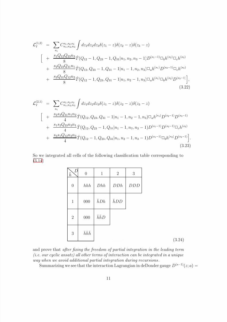
So we integrated all cells of the following classification table corresponding to(3.14)

hD

0 1 2 3

0

1

2

3

hhh Dhh DDh DDD

000

000

hhh

hDh hDD

hhD

(3.24)

and prove that after fixing the freedom of partial integration in the leading term (i.e. our cyclic ansatz) all other terms of interaction can be integrated in a uniqueway when we avoid additional partial integration during recursions.

Summarizing we see that the interaction Lagrangian in deDonder gauge D(s−1)(z; a) =

11



0 can be expressed as a sum

LdD

I (h(s)

) =

3 j=0

L(0,j)I (h

(s)

). (3.25)

and it is nothing else than the first column of this table. Therefore (3.19) meansthat in deDonder gauge the traces of the HS fields decouple from the fields as they do in the free Lagrangian.

4 Classification of gauge invariant cubic vertices

From the recent literature [1], [2], [15] we can first speculatively group the cubicgauge invariant vertices into four classes depending on the number of Weyl ten-sors they contain. In [15] vertices with (say even) spins s1, s2, s3 were explicitlyconstructed e.g. for the case 4, 4, 2, and the result was presented in a form whichwas linear in the (linearized) Weyl tensor of the minimal spin. In the remainingbracket of terms a second Weyl tensor (say for spin 2) is apparently not hidden.In [2] the ensemble of vertices constructed contain those of the spin type 2s,s,s,and these are quadratic in the (linearized) Weyl tensor of the spin s field. In allthese cases the number of derivatives is minimal and equals ∆ = s3+s2−s1, wheres1 is the minimal spin. In this section we order the spins such as s1 ≤ s2 ≤ s3,because the smaller spins give rise to the Weyl tensors, and these are representedby differential operators acting from left to right. Abandoning the constraint of

minimality on the number of derivatives, one can construct vertices from threeRiemann tensors by contraction having ∆BI = s1 + s2 + s3 derivatives § (Born-Infeld interaction). Finally a selfinteracting vertex of spin type s,s,s has beenderived in [1] for s = 4, which apparently did not factorize into any Weyl tensorat all. If we consider only the leading order terms discussed in Section 2, the Weyltensor reduces to the Riemann tensor. The Riemann tensor for spin s gauge field[27], [28] is best defined for our purpose by the differential expression

R(s)(z; a, b) = [(a∇)(b∂ c) − (a∂ c)(b∇)]sh(s)(z; c). (4.1)

With the cyclic ansatz for a vertex of an arbitrary spin type presented in thepreceeding section, we can derive results on the factorization of the l. o. termsinto Riemann tensors. Denoting the powers of the Riemann tensors maximallyappearing by n, and letting the number of derivatives be ∆∗ ≥ ∆ we may defineclasses of vertices V n(∆∗) and characterize them in terms of the spin si. Thereremain two tasks. First we may consider all explicitly known vertices for minimalderivative number ∆ and rewrite their leading orders in terms of the cyclic nota-tion for the l. o. terms discussed in the preceeding section. This was in all cases

§This case is also described by our general formula for the case ∆ = ∆BI and the triangleinequality s1 + s2 ≥ s3

12



possible. On the other hand we can turn this issue around and derive from thecyclic ansatz of Section 1 with minimal derivative number the maximum amountof information possible on the factorization into Riemann tensors, which givesnew general insights on which spin type belongs to which class V n(∆).

We prove the following theorem: The class V 0(∆) consists of those spin typeswith s3 < 2s1, the class V 1(∆) of the spin types s3 ≥ 2s1, s2 > s1, and the classV 2(∆) of the types s3 ≥ 2s1 = 2s2 . As a corollary we obtain that V 0(∆) containsall selfinteractions.

For the proof we start from (2.4), (2.12). We obtain by replacing n1 = s1− pand summing over n2, n3

n2,n3

s1

n1, n2 − s2 + s1, n3 − s3 + s1

(∂ a∇2)n1(∂ b∇3)n2(∂ c∇1)n3

(∂ a∂ b)n3−s3+s1(∂ b∂ c)n1(∂ c∂ a)n2−s2+s1h(s1)(z1; a)h(s2)(z2; b)h(s3)(z3; c)

=

s1 p

[(∂ a∇2)(∂ b∂ c)]s1− p(∂ c∇1)s3−s1(∂ b∇3)s2−s1

{(∂ c∇1)(∂ b∂ a) + (∂ c∂ a)(∂ b∇3)} p h(s1)(z1; a)h(s2)(z2; b)h(s3)(z3; c). (4.2)

Since we want to neglect all higher order terms (such as divergences, traces andcontractions of gradients (∇i∇ j)¶), use partial integrations implied by ∇1 +∇2 +∇3 = 0, and keep only the l.o. expressions, we can in the square bracket replace(∂ b∇3) by −(∂ b∇1). Introducing two arbitrary tangential vectors e, f and thestar product we get

[(∂ b∂ a)(∂ c∇1) − (∂ c∂ a)(∂ b∇1)] p

= [(e∂ a)(f ∇1) − (f ∂ a)(e∇1] p

∗e ∗f [(e∂ b)(f ∂ c)] p

,(4.3)

where we obtained p differential operator factors acting on h(s1)(z1, a) of a Rie-mann tensor. The other s1 − p components are produced as follows.

The remaining factors in (4.2) can be reordered by

[(∂ a∇2)(∂ b∂ c)]s1− p(∂ c∇1)s3−s1(∂ b∇3)s2−s1

= [(∂ a∇2)(∂ c∇1)]s1− p(∂ b∂ c)s1− p(∂ c∇1)s3−2s1+ p(∂ b∇3)s2−s1, (4.4)

which is permitted if s3 − 2s1 ≥ 0, since p runs from 0 to s1. Then the squarebracket can be contracted in the same way with the tangential vectors e, f andneglecting a contraction (∇1∇2) as of higher order we get

[(e∂ a)(f ∇1) − (f ∂ a)(e∇1)]s1− p ∗e ∗f [(e∇2)(f ∂ c)]s1− p. (4.5)

Multiplication of the two products over the square bracket operators (4.3) and(4.5) yields the Riemann tensor

Rs1(z1; f, e) = [(e∂ a)(f ∇1) − (f ∂ a)(e∇1)]s1h(s1)(z1; a). (4.6)

¶Note that the product of derivatives (∇i∇j) in this case leads also to 2R(s)(a; b; h(s)(c; z))which is equal to R(s)(a; b; (c∇)D(s−1)) = 0 on shell due to gauge invariance of the linearizedcurvature

13



However, in the remaining factors there is still the term

(∂ c∇1)s3−2s1+ p, (4.7)

which acts on h(s1) (i.e. the Riemann tensor), but by partial integration andneglect of divergences as higher order terms, we can let it act on h(s2). Then weobtain the first Riemann tensor formula

R(s1)(z1; f, e) ∗e ∗f

s1 p=0

(−1) p

s1 p

(e∂ b) p(e∇2)s1− p(f ∂ c)s1

(∂ b∂ c)s1− p(∂ c∇2)s3−2s1+ p(∂ b∇3)s2−s1 h(s2)(z2; b)h(s3)(z3; c). (4.8)

The next construction is also intended to be a Riemann tensor for the spin s1.

For this purpose we construct a homogeneous function in b of degree s1. Usingthe appropriate factors from (4.8) we define

H (z2, z3; b,c,f ) = (f ∂ c)s1(∂ b∇3)s2−s1(∂ c∇2)s3−2s1h(s2)(z2; b)h(s3)(z3; c), (4.9)

which is homogeneous both in b and c of degree s1. Then we can perform thesum in (4.8) and get

[(e∇2)(∂ b∂ c) − (∂ c∇2)(e∂ b)]s1H (z2, z3; b,c,f ). (4.10)

Concerning the differential operator in front of H this expression looks like a

Riemann tensor R

(s1)

(z2). But a gauge transformation δh

(s2)

(z2, b) acts as

(∂ b∇3)s2−s1(b∇2)ǫ(s2−1)(z2; b) =

(s2 − s1)(∇2∇3)(∂ b∇3)s2−s1−1ǫ(s2−1)(z2; b)

+(b∇2)(∂ b∇3)s2−s1ǫ(s2−1)(z2, b). (4.11)

We conclude that only for s2 = s1 the expression (4.10) can be considered as aproper Riemann tensor. This completes the proof of the theorem.

14



5 Discussion: Towards gauge transformations

as open Lie algebras

If all spins in the cubic interaction are equal s, we can derive the first order gaugetransformation of h(s) from the r. h. s. of Noether’s equation (3.4) taken off shell

[O(F ) part of δ0ǫ(s1−1)

LI ]

=ni

C s1,s2,s3n1,n2,n3


−

s1n1

2T (Qij|n1 − 1, n2, n3)ǫ(s1−1)F (s2)h(s3)

+s1Q12n2

4T (Q12 − 1, Q23, Q31|n1, n2 − 1, n3)ǫ(s1−1)

2bF (s2)h(s3)

+s3s1Q12n2n3

4T (Q12 − 1, Q23, Q31|n1, n2 − 1, n3 − 1)ǫ(s1−1)

2bF (s2)D(s3−1)

+s1Q12Q23n3

8T (Q12 − 1, Q23 − 1, Q31|n1, n2, n3 − 1)ǫ(s1−1)

2bF (s2)2ch(s3)

+s1n1

2T (Qij|n1 − 1, n2, n3)ǫ(s1−1)h(s2)F (s3)

+s1Q12n2

4T (Q12 − 1, Q23, Q31|n1, n2 − 1, n3)ǫ(s1−1)

2bh(s2)F (s3)

+s1s2n1n2

4T (Q12, Q23, Q31|n1 − 1, n2 − 1, n3)ǫ(s1−1)D(s2−1)F (s3)

−

s1Q12Q23n3

8ˆT (Q12 − 1, Q23 − 1, Q31|n1, n2, n3 − 1)ǫ

(s1−1)2

bh(s2)2

cF (s3)

.(5.1)

If we assume moreover that the gauge transformations form a Lie algebra of powerseries in some ”coupling constant” g, we can following along the ideas of Berends,Burger and Van Dam in their classical paper [7] derive conclusions on the higherorder interactions. We sum up simple results:

(1) The arguments of these authors to show that such power series algebradoes not exist for s = 3, cannot be generalized to even spins;

(2) the quartic interaction Lagrangian is nonzero and contains 2s− 2 deriva-tives.

For a given gauge function ǫ(s−1)(z; a) the gauge transformation is a substitu-tion (classically) with expansion

h → h + δǫh = h + ∇ǫ +n≥1

gnΘn(h,h,...h; ǫ), (5.2)

with Θn depending on ǫ linearly and on h in the n’th power. Moreover we assumethat the commutator of two such transformations is given by

[δǫ, δη]h = δC (h;ǫ,η)h, (5.3)

15



with the expansion

C (h; ǫ, η) = gn≥0

gnC n(h,h,...h; ǫ, η), (5.4)

where each C n depends on ǫ and η linearly and on h in the n’th power. Assubstitutions gauge transformations are associative and their infinitesimals mustsatisfy the Jacobi identity. At order g2 this is e.g.

η,ǫ,ζ cyclic

{C 1(∇ζ ; η, ǫ) + C 0(C 0(η, ǫ), ζ )} = 0. (5.5)

The commutator can also be expanded

[δη, δǫ] = g(Θ1(∇ǫ; η) −Θ1(∇η; ǫ))+ g2{[Θ1(Θ1(h; ǫ); η)−Θ1(Θ1(h; η); ǫ)]

+ [Θ2(∇ǫ, h; η) −Θ2(∇η, h; ǫ)]

+ [Θ2(h,∇ǫ; η) −Θ2(h,∇η; ǫ)]}+ O(g3). (5.6)

Inserting this expansion into the definition of the functions C n we obtain

∇C 0(η, ǫ) = Θ1(∇ǫ; η)−Θ1(∇η; ǫ), (5.7)

∇C 1(h; η, ǫ) = Θ1(Θ1(h; ǫ); η)−Θ1(Θ1(h; η); ǫ)− Θ1(h; C 0(η, ǫ))

+ Θ2(∇ǫ, h; η)− Θ2(∇η, h; ǫ) + Θ2(h,∇ǫ; η) −Θ2(h,∇η; ǫ).

(5.8)

Assume that Θ1(h; ǫ) has been extracted from (5.1) for the case of equal spins s.Then the order of derivations in Θ1 is

♮Θ1(h; ǫ) = s− 1. (5.9)

Inserting this result into (5.5), (5.7) we obtain the number of derivations in C 0, C 1as

♮C 0(η, ǫ) = s− 2 and ♮C 1(h; η, ǫ) = 2s − 3. (5.10)

This implies ♮Θ2(h, h; ǫ) = 2s− 3. (5.11)

Consequently the quartic interaction must contain 2s− 2 derivatives. The argu-ment can be continued to still higher interactions: For n’th order interactions thenumber is (s − 2)(n − 2) + 2. This result is equivalent to introducton a scale Land dimensions in the following way

[h] = Ls−2, [∇] =1

L, (5.12)

16



with a dimensionless coupling constant g, so that each term in the power serieshas the same dimension. Note that in the case of ∆ = ∆min we obtained in theprevious sections and in [1] the same dimensions for cubic selfinteractions and afree Fronsdal’s action.

In [7] the argument was presented that for spin s = 3 a Lie algebra of gaugetransformations in the form of power series does not exist, the problem startingwith the second power. The argument was based on the term

(∂ a∇2)s−1ǫ(s−1)(z1; a)h(s)(z2; b), (5.13)

which exists in Θ1. Such term is present in fact for any spin, as can be inspectedfrom (5.1). Namely, in the fifth term of the square bracket of (5.1) (this is theunique localization) we get such expression for n1 = s, n2 = n3 = 0. In equation

(5.8) in the first line we have thus 2s − 2 derivations acting on the field h ineither term. In no other terms of (5.8) such expression appears. Therefore theymust cancel inside this line and they do cancel indeed for even spin only. Thereis in this case no obstruction of the power series algebra by these arguments. Adeeper investigation of such algebras will follow in the future.

Acknowledgements

This work is supported in part by Alexander von Humboldt Foundation under3.4-Fokoop-ARM/1059429. Work of K.M. was made with partial support of CRDF-NFSAT UCEP06/07 and CRDF-NFSAT-SCS MES RA ECSP 09 01.

References

[1] R. Manvelyan, K. Mkrtchyan and W. Ruhl, “Direct construction of a cubicselfinteraction for higher spin gauge fields,” arXiv:1002.1358 [hep-th].

[2] R. Manvelyan, K. Mkrtchyan and W. Ruhl, “Off-shell construction of sometrilinear higher spin gauge field interactions,” Nucl. Phys. B 826 (2010) 1[arXiv:0903.0243 [hep-th]].

[3] R. Manvelyan and K. Mkrtchyan, “Conformal invariant interaction of ascalar field with the higher spin field in AdS D,” [arXiv:0903.0058 [hep-th]].

[4] R. Manvelyan and W. Ruhl, “Conformal coupling of higher spin gauge fieldsto a scalar field in AdS(4) and generalized Weyl invariance,” Phys. Lett. B593 (2004) 253, [arXiv:hep-th/0403241].

[5] F. A. Berends, G. J. H. Burgers and H. van Dam, “Explicit ConstructionOf Conserved Currents For Massless Fields Of Arbitrary Spin,” Nucl. Phys.B 271 (1986) 429;

17

http://arxiv.org/abs/1002.1358



http://arxiv.org/abs/hep-th/0403241







[6] F. A. Berends, G. J. H. Burgers and H. Van Dam, “On Spin Three Selfin-teractions,” Z. Phys. C 24 (1984) 247;

[7] F. A. Berends, G. J. H. Burgers and H. van Dam, “On The Theoreti-cal Problems In Constructing Interactions Involving Higher Spin MasslessParticles,” Nucl. Phys. B 260 (1985) 295.

[8] E. S. Fradkin and M. A. Vasiliev, “On The Gravitational Interaction Of Massless Higher Spin Fields,” Phys. Lett. B 189 (1987) 89.

[9] E. S. Fradkin and M. A. Vasiliev, “Cubic Interaction In Extended The-ories Of Massless Higher Spin Fields,” Nucl. Phys. B 291 (1987) 141.M. A. Vasiliev, ”Cubic Interactions of Bosonic Higher Spin Gauge Fieldsin AdS 5”, [arXiv:hep-th/0106200]. M. A. Vasiliev, ”N = 1 Supersymmet-

ric Theory of Higher Spin Gauge Fields in AdS 5 at the Cubic Level”,[arXiv:hep-th/0206068]

[10] T. Damour and S. Deser, “Geometry of spin 3 gauge theories,” AnnalesPoincare Phys. Theor. 47, 277 (1987); T. Damour and S. Deser, “Higherderivative interactions of higher spin gauge fields,” Class. Quant. Grav. 4,L95 (1987).

[11] R. R. Metsaev, “Cubic interaction vertices for massive and massless higherspin fields,” Nucl. Phys. B 759 (2006) 147 [arXiv:hep-th/0512342];

[12] R. R. Metsaev, “Cubic interaction vertices for fermionic and bosonic arbi-

trary spin fields,” arXiv:0712.3526 [hep-th].[13] A. Sagnotti, “Higher Spins and Current Exchanges,” arXiv:1002.3388

[hep-th]; D. Francia, J. Mourad and A. Sagnotti, “Current exchangesand unconstrained higher spins,” Nucl. Phys. B 773 (2007) 203[arXiv:hep-th/0701163]; D. Francia and A. Sagnotti, “Higher-spin geometryand string theory,” J. Phys. Conf. Ser. 33 (2006) 57 [arXiv:hep-th/0601199];A. Sagnotti and M. Tsulaia, “On higher spins and the tensionless limitof string theory,” Nucl. Phys. B 682 (2004) 83 [arXiv:hep-th/0311257];D. Francia and A. Sagnotti, “On the geometry of higher-spin gauge fields,”Class. Quant. Grav. 20 (2003) S473 [arXiv:hep-th/0212185].

[14] I. G. Koh, S. Ouvry, “Interacting gauge fields of any spin and symmetry,”Phys. Lett. B 179 (1986) 115; Erratum-ibid. 183 B (1987) 434.

[15] Nicolas Boulanger, Serge Leclercq, Per Sundell, “On The Uniqueness of Minimal Coupling in Higher-Spin Gauge Theory,” JHEP 0808:056,2008;[arXiv:0805.2764 [hep-th]]. Xavier Bekaert, Nicolas Boulanger, San-drine Cnockaert, Serge Leclercq, “On Killing tensors and cubic ver-tices in higher-spin gauge theories,” Fortsch. Phys. 54 (2006) 282-290;[arXiv:hep-th/0602092].

18

























[16] A. Fotopoulos, N. Irges, A. C. Petkou and M. Tsulaia, “Higher-Spin GaugeFields Interacting with Scalars: The Lagrangian Cubic Vertex,” JHEP0710 (2007) 021; [arXiv:0708.1399 [hep-th]]. I. L. Buchbinder, A. Fo-topoulos, A. C. Petkou and M. Tsulaia, “Constructing the cubic inter-action vertex of higher spin gauge fields,” Phys. Rev. D 74 (2006) 105018;[arXiv:hep-th/0609082]. Grav. 21 (2004) S1457;

[17] M. A. Vasiliev, “Higher Spin Gauge Theories in Various Dimensions”,Fortsch. Phys. 52, 702 (2004) [arXiv:hep-th/0401177]. X. Bekaert, S. Cnock-aert, C. Iazeolla and M. A. Vasiliev, “Nonlinear higher spin theories invarious dimensions”, [arXiv:hep-th/0503128]. D. Sorokin,“Introduction tothe Classical Theory of Higher Spins” AIP Conf. Proc. 767, 172 (2005);[arXiv:hep-th/0405069]. N. Bouatta, G. Compere and A. Sagnotti, “An

Introduction to Free Higher-Spin Fields”; [arXiv:hep-th/0409068].[18] I. R. Klebanov and A. M. Polyakov, “AdS dual of the critical O(N) vector

model,” Phys. Lett. B 550 (2002) 213; [arXiv:hep-th/0210114].

[19] R. Manvelyan, K. Mkrtchyan and W. Ruhl, “Ultraviolet behaviour of higherspin gauge field propagators and one loop mass renormalization,” Nucl.Phys. B 803 (2008) 405 [arXiv:0804.1211 [hep-th]].

[20] C. Fronsdal, “Singletons And Massless, Integral Spin Fields On De SitterSpace (Elementary Particles In A Curved Space Vii),” Phys. Rev. D 20,(1979) 848;“Massless Fields With Integer Spin,” Phys. Rev. D 18 (1978)

3624.

[21] W. Ruhl, “The masses of gauge fields in higher spin field theory on AdS(4),”Phys.Lett. B 605 (2005) 413; [arXiv:hep-th/0409252]; the results presentedhere are based on extensive calculations performed by K. Lang and W. Ruhl,Nucl. Phys. B 400 (1993) 597.

[22] R. Manvelyan and W. Ruhl, “The off-shell behaviour of propagators andthe Goldstone field in higher spin gauge theory on AdS(d+1) space,” Nucl.Phys. B 717 (2005) 3; [arXiv:hep-th/0502123].

[23] R. Manvelyan and W. Ruhl, “The masses of gauge fields in higher spinfield theory on the bulk of AdS(4),” Phys. Lett. B 613 (2005) 197;[arXiv:hep-th/0412252].

[24] R. Manvelyan and W. Ruhl, “The structure of the trace anomaly of higherspin conformal currents in the bulk of AdS(4),” Nucl. Phys. B 751, (2006)285; [arXiv:hep-th/0602067].

19



























[25] R. Manvelyan and W. Ruhl, “The quantum one loop trace anomaly of thehigher spin conformal conserved currents in the bulk of AdS(4),” Nucl.Phys. B 733 (2006) 104; [arXiv:hep-th/0506185].

[26] R. Manvelyan and W. Ruhl, “Generalized Curvature and Ricci Tensors fora Higher Spin Potential and the Trace Anomaly in External Higher SpinFields in AdS 4 Space,” Nucl. Phys. B 796 (2008) 457; [arXiv:0710.0952[hep-th]].

[27] B. deWit and D.Z. Freedman, “Systematics of higher spin gauge fields,”Phys. Review D 21 (1980), 358-367.

[28] R. Manvelyan and W. Ruhl, “The Generalized Curvature and ChristoffelSymbols for a Higher Spin Potential in AdS d+1 Space,” Nucl. Phys. B 797,

371 (2008) [arXiv:0705.3528 [hep-th]].

Appendix

Proof of L(i,j)I

The expression for L(1,0)I is right if the following remaining group of terms

vanishes:

+s1n1s3

2C

(si)(ni)

[T (Qij |n1 − 1, n2, n3), (c∇3)](ǫ(s1−1)h(s2)D(s3−1) + D(s1−1)h(s2)ǫ(s3−1)) (A.1)

+s1n1s22

C (si)(ni)[T (Qij |n1 − 1, n2, n3), (b∇2)](D(s1−1)ǫ(s2−1)h(s3) − ǫ(s1−1)D(s2−1)h(s3)) (A.2)

+s2n2s1

2C

(si)(ni)

[T (Qij |n1, n2 − 1, n3), (a∇1)](D(s1−1)ǫ(s2−1)h(s3) + ǫ(s1−1)D(s2−1)h(s3)) (A.3)

+s2n2s3

2C

(si)(ni)

[T (Qij |n1, n2 − 1, n3), (c∇3)](h(s1)D(s2−1)ǫ(s3−1) − h(s1)ǫ(s2−1)D(s3−1)) (A.4)

+s3n3s2

2C

(si)(ni)

[T (Qij |n1, n2, n3 − 1), (b∇2)](h(s1)D(s2−1)ǫ(s3−1) + h(s1)ǫ(s2−1)D(s3−1)) (A.5)

+s3n3s1

2C

(si)(ni)

[T (Qij |n1, n2, n3 − 1), (a∇1)](ǫ(s1−1)h(s2)D(s3−1) −D(s1−1)h(s2)ǫ(s3−1)) (A.6)

−s1Q12s2C (si)(ni)

T (Q12 − 1, Q23, Q31|ni)ǫ(s1−1)D(s2−1)h(s3) (A.7)

−s2Q23s3C (si)(ni)T (Q12, Q23 − 1, Q31|ni)h(s1)ǫ(s2−1)D(s3−1) (A.8)

−s3Q31s1C (si)(ni)

T (Q12, Q23, Q31 − 1|ni)D(s1−1)h(s2)ǫ(s3−1). (A.9)

Indeed calculating commutators in the leading order and using relation (3.12) wesee that

(A.1) + (A.6)

= s1s2(Q23 + 1)C sin1+1,n2,n3T (Q12, Q23, Q31|n1, n2 + 1, n3)D(s1−1)h(s2)ǫ(s3−1), (A.10)

20









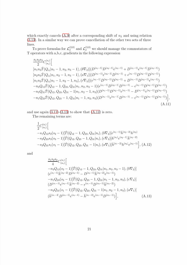
which exactly cancels (A.9) after a corresponding shift of n2 and using relation(3.13). In a similar way we can prove cancellation of the other two sets of threelines.

To prove formulas for L(2,0)I and L(3,0)

I we should manage the commutators of T operators with a,b,c, gradients in the following expression

s1s2s32

C (si)

(ni)

[n1n3T (Qij |n1 − 1, n2, n3 − 1), (b∇2)](D(s1−1)D(s2−1)ǫ(s3−1) + D(s1−1)ǫ(s2−1)D(s3−1))

[n2n3T (Qij |n1, n2 − 1, n3 − 1), (a∇1)](D(s1−1)ǫ(s2−1)D(s3−1) + ǫ(s1−1)D(s2−1)D(s3−1))

[n1n2T (Qij |n1 − 1, n2 − 1, n3), (c∇3)](ǫ(s1−1)D(s2−1)D(s3−1) + D(s1−1)D(s2−1)ǫ(s3−1))

−n3Q12T (Q12 − 1, Q23, Q31|n1, n2, n3 − 1)(ǫ(s1−1)D(s2−1)D(s3−1) − ǫ(s1−1)D(s2−1)D(s3−1))

−n2Q31ˆT (Q12, Q23, Q31 − 1|n1, n2 − 1, n3)(D

(s1−1)

D(s2−1)

ǫ(s3−1)

−D(s1−1)

ǫ(s2−1)

D(s3−1)

)−n1Q23T (Q12, Q23 − 1, Q31|n1 − 1, n2, n3)(D(s1−1)ǫ(s2−1)D(s3−1) − ǫ(s1−1)D(s2−1)D(s3−1))

,

(A.11)

and use again (3.11)-(3.13) to show that (A.11) is zero.The remaining terms are:

1

2C

(si)(ni)

−s1Q12s2(s2 − 1)[T (Q12 − 1, Q23, Q31|ni), (b∇2)]ǫ(s1−1)h(s2−2)h(s3)

−s2Q23s3(s3 − 1)[T (Q12, Q23 − 1, Q31|ni), (c∇3)]h(s1)

ǫ(s2−1)

h(s3−2)

−s3Q31s1(s1 − 1)[T (Q12, Q23, Q31 − 1|ni), (a∇1)]h(s1−2)h(s2)ǫ(s3−1)

, (A.12)

and

s1s2s34

C (si)(ni)

−n3Q12(s2 − 1)[T (Q12 − 1, Q23, Q31|n1, n2, n3 − 1), (b∇2)]

(ǫ(s1−1)h(s2−2)D(s3−1) − D(s1−1)h(s2−2)ǫ(s3−1))

−n1Q23(s3 − 1)[T (Q12, Q23 − 1, Q31|n1 − 1, n2, n3), (c∇3)]

(D(s1−1)

ǫ(s2−1)¯

h(s3−2)

− ǫ(s1−1)

D(s2−1)¯

h(s3−2)

)−n2Q31(s1 − 1)[T (Q12, Q23, Q31 − 1|n1, n2 − 1, n3), (a∇1)]

(h(s1−2)D(s2−1)ǫ(s3−1) − h(s1−2)ǫ(s2−1)D(s3−1))

, (A.13)

21



−s3s1(s1 − 1)n1

4C

(si)(ni)

Q31T (Q12, Q23, Q31 − 1|n1 − 1, n2, n3)

(δh(s1−2)h(s2)D(s3−1) + 2(∇D)(s1−2)h(s2)ǫ(s3−1))

−s1s2(s2 − 1)n2

4C

(si)(ni)

Q12T (Q12 − 1, Q23, Q31|n1, n2 − 1, n3)

(D(s1−1)δh(s2−2)h(s3) + 2ǫ(s1−1)(∇D)(s2−2)h(s3))

−s2s3(s3 − 1)n3

4C

(si)(ni)

Q23T (Q12, Q23 − 1, Q31|n1, n2, n3 − 1)

(h(s1)D(s2−1)δh(s3−2) + 2h(s1)ǫ(s2−1)(∇D)(s3−2)), (A.14)

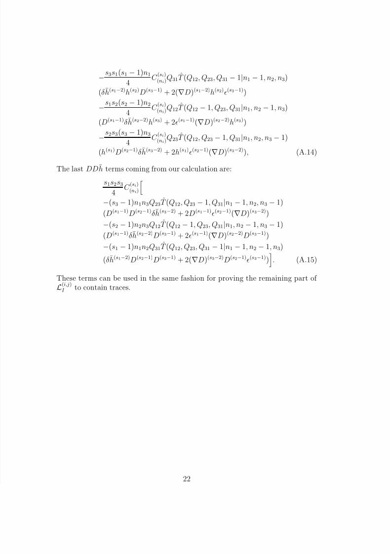
The last DDh terms coming from our calculation are:

s1s2s3

4

C (si)

(ni)−(s3 − 1)n1n3Q23T (Q12, Q23 − 1, Q31|n1 − 1, n2, n3 − 1)

(D(s1−1)D(s2−1)δh(s3−2) + 2D(s1−1)ǫ(s2−1)(∇D)(s3−2))

−(s2 − 1)n2n3Q12T (Q12 − 1, Q23, Q31|n1, n2 − 1, n3 − 1)

(D(s1−1)δh(s2−2)D(s3−1) + 2ǫ(s1−1)(∇D)(s2−2)D(s3−1))

−(s1 − 1)n1n2Q31T (Q12, Q23, Q31 − 1|n1 − 1, n2 − 1, n3)

(δh(s1−2)D(s2−1)D(s3−1) + 2(∇D)(s3−2)D(s2−1)ǫ(s3−1))

. (A.15)

These terms can be used in the same fashion for proving the remaining part of

L

(i,j)

I to contain traces.

ruben manvelyan, karapet mkrtchyan and werner ruhl-general trilinear interaction for arbitrary even...

Documents