rubinstein - simulation
TRANSCRIPT


Simulation and the Monte Carlo Method

Simulation and the Monte Carlo Method
REUVEN Y. RUBINSTEIN Technion, Israel Institute of Technology
John Wiley & Sons New York Chichester Brisbane Toronto Singapore

A NOTE TO THE READER This book has been electronicaliy reproduced from digital information stored at John Wiley &Sons, Inc. We are pleased that the use of this new technology will enable us to keep works of emluring scholarly value in print as long as there is a reasonable demand for them. The content of this book is identical to previous printings.
Copyright 0 1981 by John Wiley & Sons, lnc.
All rights reserved. Publisbcd simultaneously in Canada.
Reproduction or translation of any part of this work beyond that permitted by Sections 107 or 108 of the 1976 United Slates Copyright Act without the permission of the copyright owner is unlawful. Requests for permission or further information should be addressed to the Permissions Department, John Wiley & Sons, Inc.
Lilkruv o/congrrrr c-g k iwhbtkw Dpccc
Rubinstein, Rcuven Y. Simulation and the Monte Carlo method.
(Wiley series in probability and mathematical statistics) Includes bibliographies and index. I . Monte Carlo method. 2. Digital computer simulation. I. Title. 11. Series.
QA298.RS 5 19.2'82 8 I - 1873 ISBN Ck471-08917-6 AACRZ
10 9

To my wiJe Rina and to my friends Eitan Finkelstein and A iexandr krner - Russian refuseniks.

Preface
In the last 15 years more than 3000 articles on simulation and the Monte Carlo method have been published. There is real need for a book providing detailed treatment of the statistical aspect of these topics. This book attempts to fill this need, at least partially. I hope it will make the users of simulation and the Monte Carlo method more knowledgeable about these
It is assumed that the readers are familiar with the basic concepts of probability theory, mathematical statistics, integral and differential equa- tions, and that they have an elementary knowledge of vector and matrix operators. Sections 6.5, 6.6, 7.3, and 7.6 require more sophistication in probability, statistics, and stochastic processes; they can be omitted for a first reading.
Since most complex simulations are implemented on digital computers, a rudimentary acquaintance with computer programming will probably be an asset to the readers of this book, though no computer programs are included,
Chapter 1 describes concepts such as systems, models, and the ideas of Monte Carlo and simulation. A discussion of these concepts seems neces- sary as there is no uniform terminology in the literature. Instead of giving rigid definitions, 1 try to make clear what I mean when I use these terms. In addition to the terminology, some examples and ideas of simulation and Monte Carlo methods are given.
Chapter 2 deals with several alternative methods for generating random and pseudorandom numbers on a computer, as well as several statistical methods for testing the “randomness” of pseudorandom numbers.
Chapter 3 describes methods for generating random variables and ran- dom vectors from different probability distributions.
Chapter 4 provides a basic treatment of Monte Carlo integration, and Chapter 5 provides a solution of linear, integral, and differential equations by Monte Carlo methods. It is shown that, in order to find a solution by Monte Carlo methods, we must choose a proper distribution and present
topics.
vii

vii i PREFACE
the problem in terms of its expected value. Then, taking a sample from this distribution, we can estimate the expected value. In addition, variance reduction techniques (importance sampling, control variates, stratified sampling antithetic variates, etc.) are discussed.
Chapter 6 deals with simulating regenerative processes and in particular with estimating some output parameters of the steady-state distribution associated with these processes. Simulation results for several practical problems are presented, and variance reduction techniques are given as well.
Chapter 7 discusses random search methods, which are also related to Monte Carlo methods. In this chapter I describe how random search methods can be successfully applied for solving complex optimization problems.
The final version of this book was written during my 1980 summer visit at IBM Thomas J. Watson Research Center. I express my gratitude to the Computer Sciences Department for their hospitality and for providing a rich intellectual environment.
A number of people have contributed corrections and suBestions for improvement of the earlier draft of the manuscript, especially P. Feigin, I. Kreimer, 0. Maimon, H. Nafetz, G. Samorodnitsky, and E. Yaschin from Technion, Israel Institute of Technology, and P. Heidelberger and S. Lavenberg of IBM Thomas J. Watson Research Center. It is a pleasure to acknowledge my debt to them. I would also like to express my indebted- ness to Beatrice Shube of John Wiley & Sons and to Eliezer Goldberg of Technion for their efficient editorial guidance. Many thanks to Marylou Dietrich of IBM and to Eva Gaster of Technion for their excellent typing.
Finally, I thank the following authors and publishers for granting permission for publication of the cited material: Pages 12- 17 based on Handbook of Operations Research, Foutuktiorts and Fundamenrafs. Edited by Joseph T. Modem and Salah E. Elmagraby, Von Nostrand Reinhold Company, 1978, pp. 570-573. Pages 23-25 based on D. E. Knuth, The Art of Computer Programming: Seminumerical Algorithms, Val. 2, Addisson-Wesley, Reading, Massachu-
Pages 199-208 based on Y. R. Rubinstein, Selecting the best stable stochastic system, in Stochastic Processes and their Applications, 1980. (to appear) Pages 253-255 based on Y. R. Rubinstein and 1. Weisman, The Monte Carlo method for global optimization, Cahiers du Centre d'Etudes de Recherche Operationelle. 21, No. 2, 1979, pp. 143- 149.
setts, 1969, pp. 155- 156.

PREFACE ix
Pages 248-251 based on Y. R. Rubinstein, and A. Kornovsky, Local and integral properties of a search algorithm of the stochastic approximation type. Stochusfic Processes Appf. , 6, 1978, 129- 134.
REWEN Y. RUBINSTEIN
Ha.$2, Israel March 1981

Con tents
1. SYSTEMS, MODELS, SIMULATION, AND THE MONTE CARL0 METHODS
2.
1.1 systems, 1
1.2 Models, 3
13 Simdation and the Monte Carlo Methods, 6
1.4 A Madiine Shop Example, 12
References, 17
RANDOM NUMBER GENERATION
2.1 Introduction, 20
2.2 Coognrential Generators, 21
23 Statistical Tests of Pseudorandom Numbers, 26
2.3.1 2.3.2 2.3.3 2.3.4 Serial Test, 30 2.3.5 Run-Up-ad-Down Test, 31 2.3.6 Gap Test, 32 2.3.7 Maximum Test, 33
Chi-square Goodness-ofi Fit Te.st, 26 ~o~mogorou-Smirnou Goodness-o& Fit Test, 27 Cramer-wn Mises Goodness-of-Fit Test, 30
Exercfses, 33
References, 35

xii
3. RANDOM VARIATE GENERATION
3.1
3.2
33 3.4
35
3.6
3.7
Introduction, 38
inverse Transform Method, 39
Composition Method, 43
Acceptance-Rejection Method, 45
3.4. I 3.4.2 Multisurinte Cuse, 50 3.4.3 3.4.4 Forsythe’s Method, 56
Simulation of Random Vectors, 58
3.5, I Intvrse Transform Merhod, 58 3.5.2 Multivariate Transformation Method, 61 3.5.3 Multinormal Distribution, 65
Generating from Continuous Distributions, 67
Single- Variate Case, 45
Generalization of von Neumunn’s Method, 51
3.6. I 3.6.2 3.6.3 3.6.4 3.6.5 3.6.6 3.6.7 3.6.8 3.6.9 3.6.10
Exponentid Distribution, 67 Gamma Distribution, 71 Beta Distribution, 80 Normal Distribution, 86 Lognormal Distribution, Y I Cauchy Distribution, 91 Weibul Distribution, 92 Chi-square Distribution, 93 Student’s t-Dislribution. 94 F Distribution, 94
Generating from Discrete Distributions, 95
3.7. I Binomial Distribution, 101 3.7.2 3.7.3 Geometric Distribution, 104 3.7.4 Negatice Binomial Distribution, 104 3.7.5 Hypergeometric Distribution, 106
Exercises, 107
References, 1 1 I
Poisson Distribu t ion, I02
CONTENI S
38

CONTENTS
4. MONTE CARL0 INTEGRATION AND VARXANCE REDUCTION TECHNIQUES
4.1 Introduction, 114
4.2 Monte Carlo Integration, 115
4.2.1 4.2.2 4.2.3 4.2.4
The Hit or Miss Monte Carlo Method I15 The Sample-Mean Monte Carlo Method, I18 Efliciency of Monte Carlo Method I19 Integration in Presence qf Noise, I20
4 3 Variance Reduction Techniques, 121
4.3. I 4.3.2 4.3.3 4.3.4 4.3.5 4.3.6 4.3.7 4.3.8 4.3.9 4.3.10 4.3.JI 4.3.12
Importance Sampling, 122 Correlated Sampling. I24 Control Variates. 126 Stratified Sampling, I31 Antithetic Variates, I35 Partifion of the Region, 138 Reducing the Dimensionaliq, I40 Conditional Monte Carlo, 141 Random Quadrature Method, 143 Biased Estimators, I45 Weighted Monle Carlo Integration, 147 More about Variance Reduction (Queueing Systems and Networks), 148
Exercises, 153
References, 155
Additional References, 157
5. LINEAR EQUATIONS AND MARKOV C W N S
5.1 Simultaneous Linear Equations and Ergodic Markov Chains, 158
5.1. I 5.1.2
Adjoini System of Linear Equations, I63 Computing the Intvrse Matrix, 168
xiii
114
158

xiv CONTENTS
5.1.3 Soloing a Sysrem of Linear Equations by Simulating a Markoo Chain with an Absorbing State, 170
5.2 lntegral Equations, 173
52.1 Integral Transforms, I 73 5.2.2 5.2.3 Eigenvalue Probfem, I78
Integral Equations of the Second K i d 176
53 The DirichIet Problem, I79
Exercises, 180
References, 181
6. REGENERATIVE METHOD FOR SIMULATION ANALYSIS 183
6.1 Introduction, 183
6.2 Regenerative SimuIation, 184
6 3 Point Estimators aad Confidence Intervals, 187
6.4 Examples of Regenerative Pmceses, 193
6.4.1 A Single Seroer Queue G I / G / I , 193 6.4.2 A Repairman Modef with Spares, 195 6.4.3 A Closed Queueing Network, I97
6.5 Selecting the Best Stable Stochastic System, 199
6.6 Tbe Regenerative Method for Constrained Optimization ProMems, 248
6.7 Variance Reduction Tecbuiques, 213
6.7.1 6.7.2
Confrof Variaf es, 2 14 Common Random Numbers in Comparing Stochasric S’sfem, 224
Exercises, 2t9
References, 230
CONTENTS
7. MONTE CARL0 OPTIMIZATION
7.1
7.2
7 3
7.4
7 5
7.6
Random search Algorithms, 235
Efficiency of Random Search AlgWtthms, 241
h i and Integral Properties of Optimum Trial Random sesrd, Algorithm RS4,248 7.3.1 7.3.2
Monte Cwto Method for Globat Optimizadon, 2f2
A Closed Form Soiution for Global Optimization, Mo Optimization by Smootbd Functioaab;, 263
Appendix, 272
Exercises, 273
References. 273
Local Properires of the Algorithm, 248 iniergral Properties of the Algorithm, 251
xv
234
INDEX, 277

Simulation and the Monte Carlo Method

C H A P T E R 1
Systems, Models, Simulation, and the Monte Carlo Methods
In this chapter we discuss the concepts of systems, models, simulation and Monte Carlo methods. This discussion seems necessary in the absence of a unified terminology in the literature. We do not give rigid definitions, however, but explain what we mean when using the above-mentioned terms.
1.1 SYSTEMS
By a system we mean a set of reiated entities sometimes called componenfs or elemenrs. For instance, a hospital can be considered as rt system, with doctors. nurses, and patients a.. elements. The eiements have certain characteristics, or attributes, that have logical or numerical values. In aur example an attribute can be, for instance, the number of beds, the number of X-ray machines, skill, quantity, and so on. A number of activities (relations) exist among the elements, and consequently the elements inter- act. These activities cause changes in the system. For example, the hospital has X-ray machines that have an operator. If there is no operator, the doctors cannot have X-rays of the patients taken.
We consider both internal and external relationships. The internal relationships connect the elements within the system, while the external relationships connect the elements with the environment, that is, with the world outside the system. For instance. an internal relationship is the relationship or interaction between the doctors and nurses, or between
1
Simulation and the Monte Carlo Method R E W E N Y. RUBINSTEIN
Copyright 0 1981 by John Wiley & Sons, Inc.
2 SYSTEMS, MODELS, SI.MC'LATION, AND THE MONTE CARLO METHODS
- lnput Outpur
h System I
I I I I I I I Feedback loop I i ------------ 2
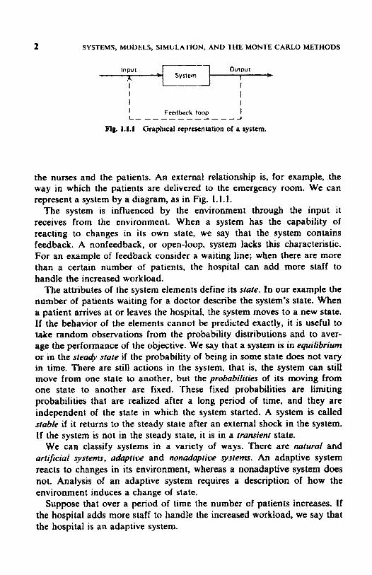
Flg. 1.1.1 Graphical representation of a system.
the nurses and the patients. An external relationship is, for example, the way in which the patients are delivered to the emergency room. We can represent a system by a diagram, as in Fig. 1.1.1.
The system is influenced by the environment through the input it receives from the environment. When a system has the capability of reacting to changes in its own state, we say that the system contains feedback. A nonfeedback, or open-loop, system lacks this characteristic. For an example of feedback consider a waiting line; when there are more than a certain number of patients, the hospital can add more staff to handle the increased workload.
The attributes of the system elements define its state. In our example the number of patients waiting for a doctor describe the system's state. When a patient arrives at or leaves the hospital, the system moves to a new state. If the behavior of the elements cannot be predicted exactly, it is useful to take random observations from the probability distributions and to aver- age the performance of the objective. We say that a system is in equilibrium or in the steady state if the probability of being in some state does not vary in time. There are still actions in the system, that is, the system can still move from one state to another, but the probabilities of its moving from one state to another are fixed. These fixed probabilities are limiting probabilities that are realized after a long period of time, and they are independent of the state in which the system started. A system is called stable if it returns to the steady state after an external shock in the system. If the system is not in the steady state, i t is in a transient state.
We can classify systems in a variety of ways. There are natural and artificial systems, ada;price and nonadaptiw sysrems. An adaptive system reacts to changes in its environment, whereas a nonadaptive system does not. Analysis of an adaptive system requires a description of how the environment induces a change of state.
Suppose that over a period of time the number of patients increases. If the hospital adds more staff to handle the increased workload, we say that the hospital is an adaptive system.

MODELS 3
1.2 MODELS
The first step in studying a system is building a model. The importance of models and model-building has been discussed by Rosenbluth and Wiener (321, who wrote:
No substantial part of the universe is so simple that it can be grasped and controlled without abstraction. Abstraction consists in replacing the part of the universe under consideration by a model of similar but simpler structure. Models.. .are thus a central necessity of scientific procedure.
A scientific model can be defined as an abstraction of some real system, an abstraction that can be used for prediction and control. The purpose of a scientific model is to enable the analyst to determine how one or more changes in various aspects of the modeled system may affect other aspects of the system or the system as a whole.
A crucial step in building the model is constructing the objective function, which is a mathematical function of the decision variables.
There are many types of models. Churchman et al. 141 and Kiviat [IS] described the following kinds:
1 Iconic models Those that pictorially or visually represent certain aspects of a system.
2 Analog models Those that employ one set of properties to represent some other set of properties that the system being studied possesses.
3 Symbolic models Those that require mathematical or logical opera- tions and can be used to formulate a solution to the problem at hand.
In this book, however. we are concerned only with symbolic models (which are also called abstract models), that is, we deal with models consisting of mathematical symbols or flowcharts. All other models (iconic, analog, verbal, physical, etc.), although no less important, are excluded from this hook.
‘There are many advantages by using mathematical models. According to Fishman (81 they do the following:
1 Enable investigators to organize their theoretical beliefs and empiri- cal observations about a system and to deduce the logical implications of this organization.
2 Lead to improved system understanding. 3 Bring into perspective the need for detail and relevance. 4 Expedite the analysis. 5 Provide a framework for testing the desirability of system modifica-
tions.

4 SYSTEMS, MODELS, SIMULATION. AND THE MONTE CARL0 METHODS
6 Allow for easier manipulation than the system itself permits. 7 Permit control over more sources of variation than direct study of a
8 Are generally less costly than the system. system would allow.
An additional advantage is that a mathematical model describes a problem more concisely than, for instance, a verbal description does.
On the other hand, there are at least three reservations in Fishman’s monograph [S], which we should always bear in mind while constructing a model.
First, there is no guarantee that the time and effort devoted to modeling will return a useful result and satisfactory benefits. Occasional failures occur because the level of resources is too low. More often, however, failure results when the investigator relys too much on method and not enough on ingenuity; the proper balance between the two leads to the greatest probability of success.
The second reservation concerns the tendency of an investigator to treat his or her particular depiction of a problem as the best representation of reality. This is often the case after much time and effort have been spent and the investigator expects some useful results.
The third reservation concerns the use of the model to predict the range of its applicability without proper qualification.
Mathematical models can be classified in many ways. Some models are srutic, other are ~+nomic. Static models are those that do not explicitly take time-variation into account, whereas dynamic models deal explicitly with time-variable interaction. For instance, Ohm’s law is an example of a static model, while Newton’s law of motion is an example of a dynamic model.
Another distinction concerns deterministic versus sfochmtic models. In a deterministic model all mathematical and logical relationships between the elements are fixed. As a consequence these relationships completely de- termine the solutions. In a stochastic model at least one variable is random.
While building a model care must be taken to ensure that it remains a valid representation of the problem.
In order to be useful, a scientific model necessarily embodies elements of two conflicting attributes-realism and simplicity. On the one hand, the model should serve as a reasonably close approximation to the real system and incorporate most of the important aspects of the system. On the other hand, the model must not be so complex that it is impossible to understand and manipulate. Being a formalism, a model is necessarily an abstraction.
Often we think that the more details a model includes the better it resembles reaIity. But adding details makes the solution more difficult and
MODELS 5
converts the method for solving a problem from an analytical to an approximate numerical one.
In addition, it is not even necessary for the model to approximate the system to indicate the measure of effectiveness for all various alternatives. All that is required is that there be a high correlation between the predic- tion by the model and what would actually happen with the real system. To ascertain whether this requirement is satisfied or not, it is important to test and establish control over the solution.
Usually, we begin testing the model by re-examining the formulation of the problem and revealing possible flaws. Another criterion for judging the validity of the model is determining whether all mathematical expressions are dimensionally consistent. A third useful test consists of varying input parameters and checking that the output from the model behaves in a plausible manner. The fourth test is the so-calied retrospective test. It involves using historical data to reconstruct the past and then determining how well the resulting solution would have performed if it had been used. Comparing the effectiveness of this hypothetical performance with what actually happened then indicates how well the model predicts the reality. However, a disadvantage of retrospective testing is that it uses the same data that guided formulation of the model. Unless the past is a true replica of the future, it is better not to resort to this test at all.
Suppose that the conditions under which the model was built change. In this case the model must be modified and control over the solution must be established. Often, it is desirable to identify the critical input parameters of the model, that is, those parameters subject to changes that would affect the solution, and to establish systematic procedures to control them. This can be done by sensitioity analysis, in which the respective parameters are varied over their ranges to determine the degree of variation in the solution of the model.
After constructing a mathematical model for the problem under consid- eration, the next step is to derive a solution from this model. There are analytic and numerical solution methods.
An analytic solution is usually obtained directly from its mathematical representation in the form of formula.
A numerical solution is generally an approximate solution obtained as a result of substitution of numerical values for the variables and parameters of the model. Many numerical methods are iterative, that is, each succes- sive step in the solution uses the results from the previous step. Newton’s method for approximating the root of a nonlinear equation can serve as an example. Two special types of numerical methods are simulation and the Monte
Carlo methods. The following section discusses these.

6 SYSTEMS, MODELS, SIMUI.ATION, AND THE MONTE CARLO METHODS
13 SIMULATION AND THE MONTE CARLO METHODS
Simulation has Iong been an important tool of designers, whether they are simulating a supersonic jet flight, a telephone communication system, a wind tunnel, a large-scale military battle (to evaluate defensive or offensive weapon systems), or a maintenance operation (to determine the optimal size of repair crews).
Although simulation is often viewed as a “method of last resort” to be employed when everything else has faiied, recent advances in simulation methodologies, availability of software, and technical developments have made simulation one of the most widely used and accepted tools in system analysis and operations research.
Naylor et al. [28] define simulation as follows:
Simulation is a numerical technique for conducting experiments on a digital computer, which involves certain types of mathematical and logicjll models that describe the behavior af business or economic system (or some com- ponent thereof) over extended periods of real time.
This definition is extremely broad, however, and can include such seemingfy unrelated things as economic models, wind tunnel testing of aircraft, war games, and business management games.
Naylor et al. f28] write:
The fundamental rationale for using simulation is man’s unceasing quest for knowledge about the future. This search for knowledge and the desire to predict the future arc as old as the history of mankind. But prior to the seventeenth century the pursuit of predictive power was limited almost entirely to the purely deductive methods of such philosophers as Plato, Aristotie. Euclid, and others.
Simulation deals with both abstract and physical models. Some simula- tion with physical and abstract models might involve participation by real people. Examples include link-trainers for pilots and military or business games. Two types of simulation involving real people deserve special mention. One is operational gaming, the other man-machine simulation.
The term “operational gaming” refers to those simulations characterized by some form of conflict of interest among players or human decision- makers within the framework of the simulated environment, and the experimenter, by observing the players, may be able to test hypotheses concerning the behavior of the individuals and/or the decision system as a whole.

SIMULATION AND THE MONTE CARL0 MhTtTflODS 7
In operational gaming a computer is often used to collect, process, and produce information that human players, usually adversaries, need to make decisions about system operation. Each player’s objective is to perform as well as possible. Moreover, each player’s decisions affect the information that the computer provides as the game progresses through simulated time. The computer can also play an active role by initiating predetermined or random actions to which the players respond.
War games and business management games are commonly discussed in operational gaming literature (see. e.g., Morgenthaler (231 and Shubik [38]).
Military gaming is essentially a training device for military leaders; it enables them to test the effects of alternative strategies under simulated war conditions. For example, the Naval Electronic Warfare Simulator, developed in the 195Os, consisted of a large analog computer designed primarily to assess ship damage and to provide information to two oppo- site forces regarding their respective effectiveness in a naval engagement [14, pp. IS, 161. The exercise, which is one form of simulation gaming, has been used as an educational device for naval fleet officers in the final stages of their training.
Business games are also a type of educational tool, but for training managers or business executives rather than military leaders.
A business game is a contrived situation which imbeds players in a simulated business environment, where they must make management-type decisions from time to time, and their choices at one time generally affect the environmental conditions under which subsequent decisions must be made. Further. the interaction between decisions and environment is determined by a refereeing process which i a not open to argument from the players [30, pp, 7.81.
In man-machine simulation there is no need for gaming. While interacting with the computer real people in the laboratory perform the data reduction and analysis.
The following two examples are drawn from Fishman (8): The Rand Systems Research Laboratory employed simulation to gener-
ate stimuli for the study of information processing centers [14, p. 161. The principal features of a radar site were reproduced in the laboratory, and by carefully controlling the synthetic input to the system and recording the behavior of the human detectors it was possible to examine the relative effectiveness of various man-machine combinations and procedures.
In 1956 Rand established the Logistics System Laboratory under U.S. Air Force sponsorship [lo]. The first study in this laboratory involved

8 SYSTEMS, MODELS, SIMULATION, AND THE MONTE CARL0 METHODS
simulation of two large logistics systems in order to compare their effec- tiveness under different management and resource utilization poticies. Each system consisted of men and machines, together with policy rules for the use of such resources in simulated stress situations such as war. The. simulated environment required a specified number of aircraft in flying and alert states, while the system’s capability to meet these objectives was limited by malfunctioning parts, procurement and transportation delays, and the like. The human participants represented management personnel, while higher echelon policies in the utilization of resources were simulated on the computer. The ultimate criteria of the effectiveness of each system were the number of operationally ready aircraft and the dollar cost of maintaining this number.
Although the purpose of the first study in this laboratory was to test the feasibility of introducing new procedures into an existing air force logistics system and to compare the modified system with the original one, the second laboratory problem had quite a different objective. Its purpose was to improve the design of the operational control system through the use of simulation.
Naylor et ai. [28] describe many situations where simulation can be successfully used. We mention some of them.
First, it may be either impossible or extremely expensive to obtain data from certain processes in the real world. Such processes might involve, for example, the performance of large-scale rocket engines, the effect of proposed tax cuts on the economy, the effect of an advertising campaign on total sales. In this case we say that the simulated data are necessary to formulate hypotheses about the system.
Secondly, the observed system may be so complex that it cannot be described in terms of a set of mathematical equations for which analytic solutions are obtainable. Most economic systems fall into this category. For example, it is virtually impossible to describe the operation of a business firm, an industry, or an economy in terms of a few simple equations. Simulation has been found to be an extremely effective tool for dealing with problems of this type. Another class of problems that leads to similar difficulties is that of large-scale queueing problems invofving multi- ple channels that are either parallel or in series (or both).
Thirdly, even though a mathematical model can be formulated to describe some system of interest, it may not be possible to obtain a solution to the model by straightforward analytic techniques. Again, eco- nomic systems and complex queueing problems provide examples of this type of difficulty. Although it may be conceptually possible to use a set of mathematical equations to describe the behavior of a dynamic system

SIMULATION AND THE MON'I'E CAR1.0 METHODS 9
operating under conditions of uncertainty, presentday mathematics and computer technoiogy are simply incapable of handling a problem of this magnitude.
Fourth, it may be either impossible or very costly to perform validating experiments on the mathematical models describing the system. In this case we say that the simulation data can be used to test alternative hypotheses.
In all these cases simulation is the only practical tool for obtaining relevant answers.
Naylor et ai. [28f have suggested that simulation analysis might be appropriate for the following reasons:
Simulation makes it possible to study and experiment with the complex internal interactions of a given system whether it be a firm, an industry, an economy, or some subsystem of one of these.
2 Through simulation we can study the effects of certain informa- tional, organizational, and environmental changes on the operation of a system by making alterations in the model of the system and observing the effects of these alterations on the system's behavior.
3 Detailed observation of the system being simulated may lead to a better understanding of the system and to suggestions for improving it, suggestions that otherwise would not be apparent.
4 Simulation can be used a.. a pedagogicai device for teaching both students and practitioners basic skills in theoretical analysis, statistical analysis, and decision making. Among the disciplines in which sirnulation has been used successfully for this purpose are business administration, economics, medicine, and law.
5 Operational gaming has been found to be an excellent means of stimulating interest and understanding on the part of the participant, and is particularly useful in the orientation of persons who are experienced in the subject of the game.
6 The experience of designing a computer simulation model may be more valuable than the actuaI simulation itself. The knowledge obtained in designing a simulation study frequently suggests changes in the system being simulated. The effects of these changes can then be tested via simulation before implementing them on the actual system.
7 Simulation of complex systems can yield valuable insight into which variables are more important than others in the system and how these variables interact.
8 Simufation can be used to expenment with new situations about which we have little or no information so as to prepare for what may happen.
1

10 SYSTEMS, MODELS, SIML;I.ATION, AND THE MONTE CARL0 METHODS
9 Simulation can serve as a “preservice test” to try out new policies and decision rules for operating a system, before running the risk of experimenting on the real system.
10 Simulations are sometimes valuable in that they afford a convenient way of breaking down a complicated system into subsystems, each of which may then be modeled by an analyst or team that is expert in that area 123, p. 373).
11 Simulation makes it possible to study dynamic systems in either real time, compressed time, or expanded time.
12 When new components are introduced into a system, simulation can be used to help foresee bottlenecks and other problems that may arise in the operation of the system 123, p. 3751.
Computer simulation also enables us to repiicate an experiment. Replica- tion means rerunning an experiment with selected changes in parameters or operating conditions being made by the investigator. In addition, computer simulation often allows us to induce correlation between these random number sequences to improve the statistical analysis of the output of a simulation. ln particular a negative correlation is desirable when the results of two replications are to be summed, whereas a positive correlation is preferred when the results are to be differenced, as in the comparison of experiments.
Simulation does not require that a model be presented in a particular format. I t permits a considerable degree of freedom so that a model can bear a close correspondence to the system being studied. The results obtained from simulation are much the same as observations or measure- ments that might have been made on the system itself. To demonstrate the principles involved in executing a discrete simulation, an example of simulating a machine shop is given in Section 1.4. Many programming systems have been developed, incorporating simulation languages. Some of them are general-purpose in nature, while others are designed for specific types of systems. FORTRAN, ALGOL, and PL/1 are examples of general-purpose languages, while GPSS, SIMSCRIPT, and SIMULA are examples of special simulation languages.
Simulation is indeed an invaluable and very versatile tool in those problems where analytic techniques are inadequate. However, it is by no means ideal. Simulation is an imprecise technique. It provides only statisti- cal estimates rather than exact results, and it only compares alternatives rather than generating the optimal one. Simulation is aiso a slow and costly way to study a problem. It usually requires a large amount of time and great expense for analysis and programming. Finally, simulation yields only numerical data about the performance of the system, and sensitivity
SIMULATION AND TlIE MOVIE CARL0 MBIIIOUS 11
analysis of the model parameters is very expensive. The only possibility is to conduct series of simulation runs with different parameter values.
We have defined simulation as a technique of performing samphng experiments on the model of the system. This general definition is often called simulation in a wide sense, whereas simulation in a nurrow sense, or stochastic simulation, is defined as experimenting with the model over time; it includes sampling stochastic variates from probability distribution [ 191. Therefore stochastic simulation is actually a statistical sampling experi- ment with the model. This sampling involves all the problems of statistical design analysis.
Because sampling from a particular distribution involves the use of random numbers, stochastic simulation is sometimes called Monte Carlo simulation. Historically, the Monte Carlo method was considered to be a technique, using random or pseudorandom numbers, for solution of a model. Random numbers are essentially independent random variables uniformly distributed over the unit interval 10, 1). Actually, what are available at computer centers are arithmetic codes for generating se- quences of pseudorandom digits, where each digit (0 througb 9) occurs with approximately equal probability (likelihood). Consequently, the sequences can model successive flips of a fair ten-side die. Such codes are called random number generators. Grouped together, these generated digits yield pseudorandom numbers with any required number of elements. We discuss random and pseudorandom numbers in the next chapter.
One of the earliest problems connected with Monte Carlo method is the famous Buffon’s needle problem. The problem is as follows. A needle of length I units is thrown randomly onto a floor composed of parallel planks of equal width d units, where d > 1. What is the probability that the needle, once it comes to rest, will cross (or touch) a crack separating the planks on the floor? It can be shown that the probability of the needle hitting a crack is P = 2l/nd. which can be estimated as the ratio of the number of throws hitting the crack to the total number of throws. In the begining of the century the Monte Carlo method was used to
examine the Boltzmann equation. In 1908 the famous statistician Student used the Monte Carlo method for estimating the correlation coefficient in his r-distribution.
The term “Monte Carlo” was introduced by von Neumann and Ulam during World War 11, as a code word for the secret work at Los Alamos; it was suggested by the gambling casinos at the city of Monte Carlo in Monaco. The Monte Carlo method was then applied to problems related to the atomic bomb. The work involved direct simulation of behavior concerned with random neutron diffusion in fissionable material. Shortly thereafter Monte Carlo methods were used to evaluate complex multidi-
12 SYSTEMS, MODELS, SIMULATION, AND THE MONTE CARL0 METHODS
mensional integrals and to solve certain integral equations, occurring in physics, that were not amenable to analytic solution.
The Monte Carlo method can be used not only for solution of stochastic problems, but also for solution of deterministic problems. A deterministic problem can be solved by the Monte Carlo method if it has the same formal expression as some stochastic process. In Chapter 4 we show how the Monte Carlo method can be used for evaluating multidimensional integrals and some parameters of queues and networks. In Chapter 5 the Monte Carlo method is used for solution of certain integral and differen- tial equations.
Another field of application of the Monte Carlo methods is sampling of random variates from probability distributions, which Morgenthaler [23] calls model sampling. Chapter 3 deals with sampling from various distribu- tions.
The Monte Carlo method is now the most powerful and commonly used technique for analyzing complex problems. Applications can be found in many fields from radiation transport to river basin modeling. Recently, the range of applications has been broadening, and the complexity and com- putational effort required has been increasing, because realism is associ- ated with more complex and extensive problem descriptions.
Finally, we mention some differences between the Monte Carlo method and simulation:
1 in the Monte Carlo method time does not play as substantial a role as it does in stochastic simulation.
2 The observations in the Monte Carlo method, as a rule, are indepen- dent. In simulation, however, we experiment with the model over time so, as a rule, the observations are serially correlated.
In the Monte Carlo method it is possible to express the response as a rather simple function of the stochastic input variates. In simulation the response is usually a very complicated one and can be expressed explicitly only by the computer program itseif.
3
1.4 A MACHINE SHOP EXAMPLE
This example is quoted from Gordon [ 11, pp. 570-5731. For better under- standing of the example an important distinction to be made is whether an entity is permanent or temporary. Permanent entities can be compactly and efficiently represented in tables, while temporary entities will be volatile records and are usually handled by the list processing technique described later.

A MACHINE SHOP EXAMPLE 13
Consider a simple machine shop (or a single stage in the manufacturing process of a more complex machine shop). The shop is to machine five types of parts. The parts arrive at random intervals and are distributed randody among the different types. There are three machines, a11 equally able to machine any part. If a machine is available at the time a part arrives, machining begins immediately. If all machines are busy upon arrival, the part will wait for service. On completion of machining the part will be dispatched to a certain destination, depending on its type, The progress of the part is not followed after it is dispatched from the shop. However, a count of the number of parts dispatched to each destination is kept.
Clearly, there are two types of elements in the system: parts and machines. There will be a stream of temporary elements, that is, the parts that enter and leave the system. There is no point in representing the different types of parts as different elements; rather, the type is an attribute of the parts. As indicated before, it is simpler to consider the group of machines as a single permanent element, having as attributes the number of machines and a count of the number currently busy. The activities causing changes in the system are the generation of parts, waiting, machining, and departing.
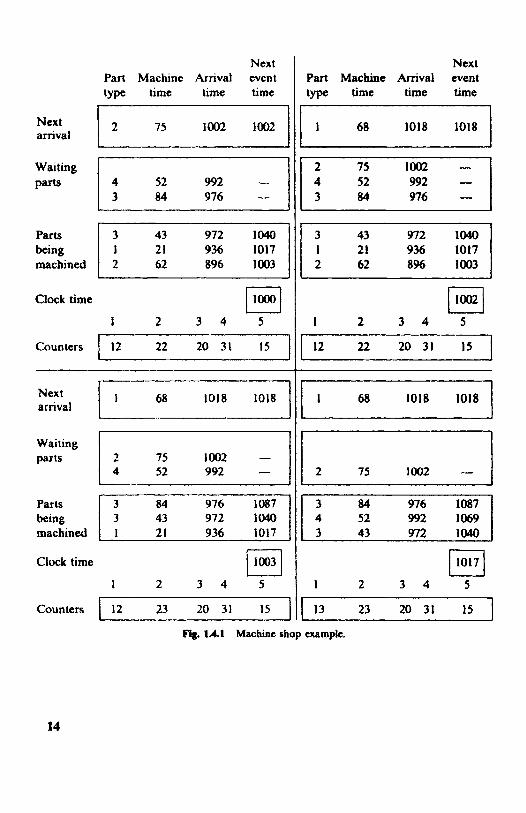
(a) System Image A set of numbers is needed to record the state of the system at any time. This set of numbers is called the syslem imge, since it reflects the state of the system. The simulation proceeds by deciding, from the system image, when the next event is due to occur and what type of event it will be; testing whether i t can be executed; and executing the changes to the image implied by the event.
The image must have a number representing clock time, an3 this number is advanced, in uneven steps, with the succession of events in the system. For each part record, there are four numbers to represent the part type, the arrival time, the machining time, and the time the part will next be involved in an event. The first three of these items are random variates derived by the methods described in Chapters 3 and 4. The next event time, in generaI, depends on the state of the system, and must be derived as the simulation proceeds.
The organization used for the system image is illustrated in Fig. 1.4.1. There are four frames in this figure, representing successive states of the system. The frames are read from left to right and from top to bottom. The frame in the top left corner is the initial state. The description of the system image is made in terms of that particular frame.
Next Part Machine Arrival event type time time time
Parts
machined being
Next 1 2 75 I002 1002 1 amval
3 43 1 21 2 62 896 1003
1 1
Waiting
Clock time
1 2 3 4 5
Counters I 12 22 20 31 I5 I
1 68 1018 1018 Next arrival
Waiting parts
being machined 936 1017
Clock time
1 2 3 4 5
Counters 12 23 20 31 15
Next Patt Machine Arrival event type time time time
( I 68 1018 1018 I I J
84 976 - I I
62 8% 1003
r;2;;;;1 1 2 3 4 5
I 12 22 20 31 15 1
1 68 I018 1018
r----- 2 75 1002 -
43 972 1040
(10171 1 2 3 4 5
1 13 23 20 31 15 I Fig. 1.4.1 Machine shop example.
14

A MACHINE SHOP EXAMPLE 15
The top line of the system image represents the part due to enter the system next. As shown here, it is a type 2 part, will require 75 minutes of machining, and is due to arrive at time 1002. This, of course, is also its next event time.
Below the next amval listing is an open-ended list of the parts that have amved and are now waiting for service. Currently, there are two waiting parts. As indicated, they are listed in order of arrival. Because the waiting parts are delayed, it is not possible to predict a next event time for them. It is necessary to see whether there is a waiting part when a machine finishes, and to offer service to the first part in the waiting line.
The next rows of numbers represent the parts now being machined, in this case limited to three. Once machining begins, the time to finish can be derived and entered as the next event time. Three parts are occupying the machines at this time and they have been listed in the order in which they will finish. Finally, a number represents the clock time, here set to an initial value of 1O00, and there are five counters showing how many parts of each type have been completed. Note that it is not customary to precalculate all the random variates. Instead, each is calculated at the time it is needed, so a simulation program continually switches between the examination and manipulation of the system image and the subroutines that calculate the random variates.
(b) The Simulation procesS Looking now at the system image in Fig. 1.4.1, assume all events that can be executed up to time loo0 have been processed. It is now time to begin one more cycle. The first step is to find the next potential event by scanning all the event times. Because of the ordering of the parts being machined, it is, in fact, necessary only to compare the time of the next arrival with the first listed time in the machining section. With the numbers shown in frame I , the next event is the arrival of a part at time 1002, so the clock is updated to this time in the second frame.
The arriving part finds all machines busy and must join the waiting line. The successor to the part just arrived is generated and inserted as the next future arrival, due to arrive at time 1018. Another cycle can now begin. The next event is the completion of machining a part at time 1003. The third frame of Fig. 1.4.1 shows the state of the system at the end of this event. The clock is updated to 1003 and the finished part is removed from the system, after incrementing by 1 the counter for that part type. There is a waiting part, so machining is started on the first part in the waiting line, and its next event time, derived from the machining time of 84, is calculated as 1087. In this case the new part for machining has the largest

16 SYSTEMS, MODELS, SIMULATION, AND THE MONTE CARLO METHODS
finish time, and it joins the end of the waiting line. The records in the waiting line and the machine segment are all moved down one line. There is tpen another completion at 1017 that, as before, leads to a counter being increment4 and service being offered to the first part in the waiting line. In this case, however, the machining time is short enough for the new part to finish ahead of one whose machining started earlier, so, instead of being the last listed part, the new part becomes the second in the list. This is shown in the last frame of Fig. 1.4.1.
(c) Statistics Gathering The purpose of the simulation, of course, is to learn something about the system. In this case only the counts of the number of completed parts by type have been kept. Depending upon the purpose of the simulation study, other statistics could be gathered. Simuia- tion language programs include routines for collecting certain typical statistics. Among the commonly used types of statistics are the following:
1 Counts Counts give the number of elements of a given type or the number of times some event occurred.
2 Utiihtion OS equipment This can be counted in terms of the fraction of time the equipment is in use or in terms of the average number of units in USE.
3 Distributions This means distributions of random variates, such as processing times and response times. together with their means and stan- dard deviations.
(d) LLst Processing In the machine shop example i t was convenient to describe the records as though they were located in one of three places, corresponding to whether they represented parts that were aniving, wait- ing, or being processed. The simulation was described in terms of moving the records from one place to the next, possibly with some resorting. A computer program that used this approach would be very inefficient because of the large amount of data movement involved. Much better control and efficiency are obtained by using list processing. With this technique each record consists of a number of contiguous words (or bytes), some of which are reserved for constructing a list of the records. Each record contains, in a standard position, the address of the next record in the list. This is called a pointer. A special word, called a header, located in a known position, contains a pointer to the first record in the list. The last record in the list has an end-of-list symbol in place of its pointer. If the list happens to be empty, the end-of-list symbol appears in the header. The pointers, beginning from the header, place the records in a specific
order, and allow a program to search the records by following the chain of

REFERENCES 17
pointers. These lists, in fact, are usually called chains. There may be another set of pointers tracing through the chain from end to beginning so that a program can move along the chain in either direction. It is also possibie for a record to be on more than one chain, simply by reserving pointer space for each possible chain.
Removing or adding a record, or reorganizing the order of a chain now becomes a matter of manipulating pointers. To remove C from a chain of the records A, B, C, D, . . . , the pointer of B is redirected to D. If the record is being discarded, its storage space would probably be returned to another chain from which it can be reassigned later. To put the record Z between B and C, the pointer of B is directed to 2 and the pointer of Z is set to indicate C . Reordering a chain consists of a series of removals and insertions.
As can be seen, list processing does not require that records be physi- cally moved. It therefore provides an efficient way of transferring records from one category to another by moving them on and off chains, and it can easily manage lists that are constantly changing size; these are two properties that are very desirable in simulation programming. Therefore list processing is used in the implementation of all major discrete system simulation languages, including the GPSS and SIMSCRIF'T simulation programs.
REFERENCES
I Ackoff, R. L., Towards a system of systems concepts, MaMge. Sei., 17, 19771, 661-671. 2 Burt, I. M., D. P. Graver, and M. Perlas, SimpIe stochastic networks: Some problem
and procedures, Nav. Res. I q i s r . Qwr:. . 17, 1970, 439-459. 3 Chorafas, D. N., System and Sinairtion. Acadrmic, New York, 1%5. 4 Churchman, C. W.. R. L. Ackoff, and E. L. Amoff, Introdttction to Operotionr Research,
Wilcy, New York, 1959. 5 bshaff , J. R. and R. L. Sisson, Design and Use of Computer SimuIation Modeis,
Macmillan, New York, 1970. 6 Frmakov. J. M., Monte Carlo Method and Rdated Questions, Nauka, Moskow, 1976 (in
Russian). 7 Evans, G. W., G. F. Wallace, and G. L. Sutherland, Simulation Using Digital Conlpurets,
hentice-Hall, Engiewood Cliffs, New Jersey, 1967. 8 Fishman. G. S.. Concepts and Merho& in Discrete Ewnt Digital Simulation. Wiley, New
Ymk, 1973. 9 Fishman, G. S., Principles o/ Discrete Ewnr Simuiation, Witey, New York, 1978.
10 Gcisler, M. A., The use of man-machine simulation for support planning, N a n Res. Logist. Quart., 7, 1960, 421-420.
I I Gordon, G., System Simulation. Prentice-Hall. Englewood Ciiffs, New Jascy, 1%9.

1% SYSTEMS, MODELS, SIMULATION, AND THE MONTE CARLO METHODS
12 H o n a k A of Operotions Research, Founaiz!ionr and F d m e d s , edited by J. J. Modern and S. E. Elmagraby, Van Nostrand Reinbold. New Yo&, 1978.
13 Hammersley, I. M. and D. C. Handscomb. Monte Carlo Method?, Wiley, New York; Metbucn, London, 1964.
14 Hannan, H. H., Simulation: A survey, Report SP-260. System Development Corpora- tion, Santa Monica, California. 1961.
IS Hillier. F. S. and G. J. Liebeman. Intmokction to Operoriw R d , Holden-Day, San Francisco, California 1968, Cbaptcr 14.
16 Hollingdde, S. H. (Ed.), Digirol Simdotion in oiprrorions Research, American HJcVier, New York. 1967.
17 10M Corporation, Biblirrgrcqolry on Simularion, Form No. 320.0924, 112 East Post Road, White Plains. New York, 1966.
18 Kiviat, P. J., Digital Computer Simuiotion: Modcling Conccp~, Report RM-5378-PR The Rand Corporation, Santa Monica, California, 1967.
I9 Kkinen, J. P. C., Staristicul Techniques in Sintulnrion, Part I, Marcel Decker. New York, 1974.
20 Lcwis. P. A. W., Large-scale Computer-Aided Statistical Mathematics, Naval Post- graduate School, Mooterey, California, in Proc. Contpuler Science and Sfarirtics: 6fh AMWI Syw. IwerJoce, Western Periodical CO., Hollywood, California, 1972.
21 Lucas. H. C., Performance evaluation and monitoring, Conput. Swu., 3, 1971.79-91. 22 Maid. H. and G. Gnugooli, Simulation oj Discrere Stocktic @stem, Science Research
Associates, Palo Alto, Califoraia, 1972. 23 Morgenthaler, G. W., The theory and application of simulation in Operations research,
in Progress in Opematiom Reseorch, edited by R. L. Ackoff, Wiky, New York, 1961. 24 M c h d . J. (Ed.). S i d t i o n , Mffiraw-Hill, Near York. 1968. 25 McMillan, C., Jr., and R. Coourles, S’sremr Anabsis: A CoyDuter Approach to Decision
MOdeLr, R c W cd., Richard D. Ervin. Homewood, lllhoiis. 1965. 26 Mikaifov, G. A., Some Problems in ripe 7 h t y of the Monte-Corlo Method, Nauka,
Novasibink, U.S.S.R.. 1974 (in Russian). 27 Mitt. I. H. and J. G. Cox, &enria& ojSimulation, Rentice-HaII, Engkwood ClifFs. New
Jersey. 1968. 28 Nayior, T. J., J. L. Ealiotfy, D. S. Burdick, and K. Chu, Conlpwcr Simvlotion Techniques,
Wiley, New York, 1966. 29 Naylor, T. J., Campurer Simulation Experiments with MOdeLt o j fi&c Systemr, Wiley.
New York, 1971. 3Q Proc. Cot$. Businem Games, sponsored by the Ford Foundation and Schooi of Business
Administration, Tulane Univmity, April 26-28, 1961. 31 Ueirman, J., Conlpufer Simularion Applications: DiscreteEmt Sinnclarionjur rhe Sywhesis
und Ana&sis o/ Complex @srem, Wiky, New Yo&, 1971. 32 Roacnbluth, A. and N. Wiener, The role of models in scicact, Phiios. Sci., Xn, No. 4,
33 Smith, J., Computer Simulation Models, Hafncr. New Yo&, 1968. 34 Sobol, J. M.. Compurarionai Method of Monte C d o , Nauka, M d o w , 1973 (in Russian). 35 Sbreider, Y. A. (Ed.), Method of Sroiisricol Tating: Monte Curio Method, Elsevier,
Amsterdam, 1964.
Oct. 1945,316-321.

REFERENCES 19
36 Stephenson, R. E., Conqpufer Simwlatron for Engineers, Harcourt Brace Jovanovitch, New York, 1971.
37 Shubik, M., On gaming and game theory, Manage. Sci., Professional Series, 18, 1972, 37- 53.
38 Shut&, M.. A Preliminuq Bibliography on Gaming, Department of Administrative Sciences, Yak University, New Haven, Connecticut, 1970.
39 Shubik, M.. Bibliography on simulation. gaming, artificial intelligence and allied topics, J . Amer. Star. Asroc., 9, 1960, 736-751.
40 Twher, K. D., The Art of Simulation, D. Van Nostrand, Princeton, New Jersey, 1963. 41 Yakowitz, S. J . , Contpurorional Probabilip and Simulation, Addison-Wesley, Reading,
Massachusetts, 1977.
C H A P T E R 2
Random Number Genera tion
2.1 INTRODUCIlON
In this chapter we are concerned with methods of generating random numbers on digital computers. The importance of the random numbers in the Monte Carlo method and simulation has been discussed in Chapter 1. The emphasis in this chapter is mainly on the properties of numbers associated with uniform random variates. The term rondom number is used instead of uniJorm random number. Many techniques for generating ran- dom numbers have been suggested, tested, and used in recent years. Some of these are based on random phenomena, others on deterministic recur- rence procedures.
Initially, manual methodr were used, including such techniques as coin flipping, dice rdling, card shuffling, and roulette wheeIs. It was believed that only mechanical (or electronic) devices could yield “truly” random numbers. These methods were too slow for general use, and moreover, sequences generated by them could not be reproduced. Shortly following the advent of the computer it became possible to obtain random numbers with its aid. One method of generating random numbers on a digital computer consists of preparing a table and storing it in the memory of the computer. In 1955 the RAND Corporation published [46] a well known table of a million random digits that may be used in forming such a table. The advantage of this method is reproducibility; its disadvantage is its lack of speed and the risk of exhausting the table.
In view of these difficulties, John von Neumann (561 suggested the mid-square method, using the arithmetic operations of a computer. His idea was to take the square of the preceding random number and extract the
20
Simulation and the Monte Carlo Method R E W E N Y. RUBINSTEIN
Copyright 0 1981 by John Wiley & Sons, Inc.

2.2 CONGRUENTIAL GENERATORS 21
middle digits; for example, if we are generating four-digit numbers and arrive at 5232, we square it, obtain 27,373,824; the next number consists of the middle four digits-namely, 3738-and the procedure is repeated. This raises a logical question: how can such sequences, defined in a completely deterministic way, be random? The answer is that they are not really random, but only seem so, and are in fact referred to aspseudoran- dom or quasi-random; still we Cali them random, with the appropriate reservation. Von Neumann’s method likewise proved slow and awkward for statistical analysis; in addition the sequences tend to cyclicity, and once a zero is encountered the sequence terminates.
We say that the random numbers generated by this or any other method are “good” ones if they are uniformly distributed, statistically independent, and reproducible. A good method is, moreover, necessarily fast and requires minimum memory capacity. Since all these properties are rarely, if ever, realized, some compromise must be found. The congruential methods for generating pseudorandom numbers, discussed in the next section, were designed specifically to satisfy as many of these requirements as possible.
2 2 CONGRUENTIAL GENERATORS
The most commonly used present-day method for generating pseudoran- dom numbers is one that produces a nonrandom sequence of numbers according to some recursive formula based on caiculating the residues modulo of some integer m of a linear transformation. It is readily seen from this definition that each term of the sequence is available in advance, before the sequence is actually generated. Although these processes are completely deterministic, it can be shown [31] that the numbers generated by the sequence appear to be uniformly distributed and statistically inde- pendent. Congruential methods are based on a fundamental congruence relationship, which may be expressed as 1321
X,+,-(uX,+c)(modm), i 5 1, ..., n, (2.2.1)
where the mult@lier a, the incremnl c, and the modulus m are nonnegative integers. The modulo notation (mod m ) means that
X,,, = a x , + c - mk,, (2.2.2)
where k, = [(ax, + c ) / m J denotes the largest positive integer in (ax, + Given an initial starting value X, (also called the seed), (2.2.2) yields a
congruence relationship (modulo m) for any value i of the sequence { X,}.
c ) / m -

22 R A m M NUMBER GENERATION
Generators that produce random numbers according to (2.2.1) are called mixed congruential generators. The random numbers on the unit inverval (0,l) can be obtained by
Xi q==- m
(2.2.3)
Clearly, such a sequence will repeat itself in at most m steps, and will therefore be periodic. For example, let a = c = X, = 3 and m = 5; then the sequence obtained from the recursive formula XI+, 5 3XI + 3(mod 5 ) is XI = 3,2,4,0,3.
It follows from (2.2.2) that Xi < m for all i. This inequality means that the period of the generator cannot exceed m, that is, the sequence X, contains at most m distinct numbers (the period of the generator in the example is 4, while m = 5).
Because of the deterministic character of the sequence, the entire se- quence recurs as soon as any number is repeated. We say that the sequence “gets into a loop,” that is, there is a cycle of numbers that is repeated endlessly. It is shown [3l] that all sequences having the form X,+ , = f ( X l ) “get into a loop.” We want, of course, to choose m as large as possible to ensure a sufficiently large sequence of distinct numbers in a cycle.
Let p be the period of the sequence. When p equals its maximum, that is, whenp = m, we say that the random number generator has a fullperiod. I t can be shown [31] that the generator defined in (2.2.1) has a full period, m, if and only if:
I c is relatively prime to m , that is, c and m have no common divisor. 2 u = I(mod g ) for every prime factor g of m. 3 u = I(mod 4) if m is a multiple of 4.
Condition 1 means that the greatest common divisor of c and m is unity. Condition 2 means that CI - g [ a / g ] + I . Let g be a prime factor of m; then denoting K = [ a / g ] , we may write
a = 1 + g k . (2.2.4)
Condition 3 means that a * 1 + 4[ a/4] (2.2.5)
if m/4 is an integer.
Xi+ I lies between the values Greenberger [ 19) showed that the correlation coefficient between X i and
i-(Z)(l-;)*-. U
m
and that its upper bound is achieved when a = m ’ / * irrespective of the value of c.

2.2 CONORUENTIAL GENERATORS 23
Since most computers utilize either a binary or a decimal digit system, we select m = 2@ or m = lop, respectively where denotes the word-length of the particular computer. We discuss both cases separately in the following.
For a binary computer we have from condition 1 that m = 2@ guarantees a full period. It follows also from (2.2.1) that, for m = 2#, the parameter c must be odd and
a = I(mod4), (2.2.6)
which can be achieved by setting a = 2 ' + l , r l 2 .
It is noted in the literature [25, 35, 44) that good statistical results can be achieved while choosing m = 235, a = Z7 + I , and c = I.
For a decimal computer m = lop. In order to generate a sequence with a full period, c must be a positive number not divisible by g = 2 or g = 5, and the multiplier a must satisfy the condition a =- )(mod 20), or alternatively, a = lo'+ 1, r > I .
Satisfactory statistical results have been achieved f 11 by choosing a = 101, c = 1, r 2 4. In this case X, had little or no effect on the statistical properties of the generated sequences.
The second widely used generator is the multiplicatiw generator X I + , =aX,(modm), (2.2.7)
which is a particular case of the mixed generator (2.2.1) with c = 0. I t can be shown [ I , 2, 5, 311 that, generally, a f i l l period cannot be
achieved here, but a maximal period can, provided that X, is reIatively prime to m and u meets certain congruence conditions.
For a binary computer we again choose m = 2@ and it is shown [31] that the maximal period is achieved when u - 8r 2 3. Here r is any positive integer.
The procedure for generating pseudorandom numbers on a binary computer* can be written as:
1 Choose any odd number as a starting value X,. 2 Choose an integer a = 8r 5 3, where r is any positive integer.
Choose a close to 2@/* (if /3 = 35, a = 2"+ 3 is a good selection). 3 Compute Xi, using fixed point integer arithmetic. T h i s product will
consist of 28 bits from which the high-order /3 bits are discarded, and the low-order /3 bits represent Xi.
4 Calculate V , = X , / 2 @ to obtain a uniformly distributed variable.
*This procedure and the one that follows arc reproduced almost verbatim from Ref. 31.

24 RANDOM NUMBER GENERATION
5 Each successive random number X,, , is obtained from the lowsrder bits of the product ax,.
For a decimal computer m = loB. I t is shown in Ref. 49 that the maximal period is achieved when a = 200r %+p, where r is any positive integer and p is any of the following 16 numbers: (3, 11, 13, 19, 2 I , 27,29,37,53,59,61,67,69,77,83,9 1). The procedure for generating ran- dom numbers on a decimal computer can be written as:
1 Choose any odd integer not divisible by 5 as a starting value A’,. 2 Choose an integer a = 2 0 r 2 p for a constant multiplier, where r is
any integer and p is any of the values 3, 11, 13, 19, 21, 27, 29,37,53,59,61,67,69,77,83,91. Choose u close to IOfl’’. (If p- 10, Q = lO0,OaO 2 3 is a good selection.)
3 Compute ax, using fixed point integer arithmetic. This product will consist of 28 digits, from which the high-order p digits are discarded, and the low-order digits are the value of XI. Integer multiplication instructions automatically discard the high-order digits.
4 The decimal point must be shifted p digits to the left to convert the random number (which is an integer) into a uniformly distributed variate defined over the unit interval U, = X,/108.
5 Each successive random number X, , I is obtained from the low-order dig& of the product ax,.
Another type of generator in which A’,,, depends on more than one of the preceding values is the additive congruential generator [ 171
X,+ ,~X,+X,- , (modm), k = 1,2 ,..,, i - 1. (2.2.8)
In the particular case k = I we obtain the well known Fibonacci sequence, which behaves like sequences produced by the multiplicative congruential method with a = (1 + *)/2. Unfortunately, a Fibonacci sequence is not satisfactorily random, but its statistical properties improve as k increases.
RESUME: We have seen that a sequence of pseudorandom numbers produced by a congruential generator is completely defined by the numbers X,, a, c, and m. In order to obtain satisfactory statistical results our choice must be based on the following six principles.:
1 The number X, may be chosen arbitrarily. If the program is run several times and a different source of random numbers is desired each time, set X , equal to the last value attained by X on the preceding run, or (if more convenient) set X, equal to the current date and time.
*These six principles are reproduced by permission from Knuth [31, pp. 155-1561.

2.2 CONGRUENTIAL GENERATORS 25
2 The number m should be large. It may conveniently be taken as the computer's word length, since this makes the computation of (aX + c) (modm) quite efficient. The computation of (ax + cxmodm) must be done exactly, with no roundoff error.
3 If m is a power of 2 (i.e., if a binary computer is being used), pick a so that a(mod 8) = 5. If m is a power of 10 (i.e., if a decimal computer is being used), choose a so that a(mod 200) = 21. This choice of a, together with the choice of c given below, ensures that the random number generator will produce all m different possible values of X before it starts to repeat.
preferably larger than m/100, but smaller than m - 6. The best policy is to take some haphazard constant to be the multiplier, such as a = 3,141,592,621 (which satisfies both of the conditions in 3).
5 The constant c should be an odd number when m is a power of 2 and, when m is a power of 10, should also not be a multiple of 5.
6 The least significant (right-hand) digits of X are not very random, so decisions based on the number X should always be primarily in- fluenced by the most significant digits. I t is generally better to think of X as a random fraction X / m between 0 and I , that is, to visualize X with a decimal point at its left, than to regard X as a random integer between 0 and m - 1. To compute a random integer between 0 and k - 1, we would multiply by k and truncate the result.
4 The multiplier a should be larger than
Finally, we present in this section the IBM System/360 Uniform Random Number Generator, a multiplicative congruential generator that utilizes the full word size, which is equal to 32 bits with 1 bit reserved for algebraic sign. Therefore an obvious choice for m is 23'.
A pure congruential generator (c = 0) with m = 2k (k > 0) can have a maximum period length of m / 4 . Thus the maximum period length is 23'/4 = 229. The period length also depends on the starting value. When the modulus m is prime, the maximum possible period length is m - 1. The largest prime less than or equal to 23' is Z3' - 1. Hence, if we choose m = Z3' - 1, the uniform random number generators will have a maximum period length of m - 1 = 23' - 2, which is only the upper bound on the period length. The maximum period length depends on the choice of the multiplier. Note that the conditions ensuring a maximum period length do not necessarily guarantee good statistical properties for the generator, although the choice of the particular multiplier 7' does satisfy some known conditions regarding the statistical performance of the generated sequence. The System/360 Generator can be described as follows. Choose any

26 RAN UOM NUMBER GENERATION
A',> 0. For n > 1,
The random numbers are (see (2.2.3)) U, = X,,/@' - I). The results of the statistical tests of the System/360 Uniform Random
Number Generator indicate that it is very satisfactory. Versions of this generator are used in the IBM SL/MATH package, the IBM version of APL, the Naval Postgraduate School random number generator package LLRANDOM, and the International Mathematics and Statistics Library (IMSL) package. The generator is also used in the simulation programming language SIMPL/I. The assembly language subroutines GGLl and GGL2 of IBM Corporation (1974) also implement this generator, as well as the FORTRAN subroutine GGL.
X,,=75Xn-,(mod23'- I ) = 16,807Xn-,(mod23'- 1).
23 STATISTICAL TESTS OF PSEUDORANDOM NUMBERS
In this section we describe some statistical tests for checking independence and uniformity of a sequence of pseudorandom numbers produced by a computer program. As mentioned earlier, a sequence of pseudorandom numbers is completely deterministic, but insofar as it passes the set of statisticai tests, it may be treated as one of "truly" random numbers, that is, as a sample from %(O, I). Our object in this section is to provide some idea of these tests rather than present rigorous proofs. For a more detailed discussion of this topic the reader is referred to Fishman [ 111 and Knuth [311.
23.1 chi-square Gooduess-of-Fit Test The chi-square goodness-of-fit test, proposed by Pearson in 1900, is
perhaps the best known of all statistical tests. Let X,, . . . , X , be a sample drawn from a population with unknown
cumulative distribution function (c.d.f.) F,(x). We wish to test the null hypothesis
H, : F,(x) = Fo(x), for all x ,
where F,(x) is a completely specified c.d.f., against the alternative
H, : F , ( x ) + Fo(x) , for some x .
Assume that the N observations have been grouped into k mutually exclusive categories, and denote by N, and Np; the observed number of trial outcomes and the expected number for the j t h category, j = 1, . . . , k, respectively, when H, is true.

2.3 STATISTICAL TESTS OF PSEUDORANDOM NUMBERS 27
The test criterion suggested by Pearson uses the following statistic:
(2.3.1)
which tends to be small when H, is true and large when Ha is false. The exact distribution of the random variable Y is quite complicated, but for large samples its distribution is approximately chi-square with k - I de- grees of freedom [ 151.
Under the Ho hypothesis we expect P(Y > = a, (2.3.2)
where a is the significant level, say 0.05 or 0.1; the quantile xt...,, that corresponds to probability 1 - -a is given in the tables of chi-square distribution.
When testing for uniformity we simply divide the interval [O, I ] into k nonoverlapping subintervals of length l/k so that Np,? = N / k , In this case we have
(2.3.3)
and (2,3.2) can again be applied for testing random number generators. To ensure the asymptotical properties of Y it is often recommended in
the literature to choose N > Sk and k > IOOO, where k = 28 and k = loa for a binary and a decimal computer, respectively.
23.2 KolmogMav-Smlmav Coodness-of-Fit Test
Another test well known in statistical literature is the one proposed by Kolmogorov and developed by Smirnov.
Let X,, ..., X w again denote a random sample from unknown c.d.f. Fx( x). The sample cumulative distributive function, denoted by F N ( x ) , is defined as
FN( x ) = -(number of X, less than or equal to x) I N
where I ( - X) is the indicator random variable (r.v.) that is,
(2.3.4)
For fixed x , F N ( x ) is itself an r.v., since it is a function of the sample.

28 RANDOM NUMBER GENERATION
Let us show that F N ( x ) has the same distribution as the sample mean of a Bernoulli distribution, namely f" F N ( x ) = ~ ] = ( ~ ) [ F I ( ~ ) ] ~ [ I - F ~ ( x ) ] ~ - ~ . k (2.3.5)
Denote V;: = 4- oo,x)( X i ) ; then has a Bernoulli distribution with parame- ter P(V, = I ) = P(Xi I x ) = F,(x). Since Zi", ,V,. has a binomial distribu- tion with parameters N and Fx(x) , and since F N ( x ) = ( I / N ) Zf-,Y, the result follows immediately.
From (2.3.5) we see that
(2.3 -6)
varF,(x) =TF,(X)[ I - F, (x) ] , (2.3.7)
Equations (2.3.6) and (2.3.7) show that, for fixed x , FN(x) is an unbiased and consistent estimator of F,(x) irrespective of the form of F,(x). Since FN( x) is the sample mean of random variables 4- o,x)( Xi), i = 1, . . . , N, it follows from the central-limit theorem that f " ( x ) is asymptotically nor- mally distributed with mean F,(x) and variance (l/N)F'(x)[ 1 - F(x)] . We are interested in estimating F'(x) for every x (or rather, for a fixed x ) and in finding how close F,(x) is to F,(x) jointly over all values x.
and 1
The result
lim P [ sup IF,(^) - ~ , . ( x ) l > e ] = o (2.3.8) N-03 - s o < x < m
is known as the Gliwnko-Cantelli theorem, which states that for every E > 0 the step function F,(x) converges uniformly to the distribution function F'(x). Therefore for large N the deviation IFN(x) - F,(x)I between the true function F,(x) and its statistical image F N ( x ) should be small for all values of x.
The random quantity D, = SUP IFN(X) - FX(X)l. (2.3.9)
which measures how far F,(x) deviates from F,(x) is called the Kolmogorm-Smirnoo one-sample statistic. Kolmogorov and Smirnov proved that, for any continuous distribution F,( x),
-oa<x<m
(2.3.10)

2.3 STATISTICAL 1ESTS OF PSEUDORANDOM NUMBERS 29
The function H ( x ) has been tabulated and the approximation was found to be sufficiently close for practical applications, so long as N exceeds 35.
The c.d.f. H ( x ) does not depend on the one from which the sample was drawn; that is, the limiting distribution of fi DN is disiribution-jiree. This fact allows D,,, to be broadly used as a statistic for goodness-of-fit,
For instance, assume that we have the random sample A',, . . . , X, and wish to test H0:F,(x)= Fo(x) for all x where Fo(x) is a completely specified c.d.f. (in our case Fo(x) is the uniform distribution in the interval (0, I)). i f Ho is true, which means that we have a good random number generator, then
is approximately distributed as the c.f.d. H( x). If Ho is false, which means that we have a bad random number
generator, then F N ( x ) will tend to be near the true c.d.f. Fx(x) ratbet than near Fo(x), and consequently ~ u p - , < , ~ ~ ( F ~ ( x ) - Fo(x)( will tend to be large. Hence a reasonable test criterion is to reject H , if
The Kolmogorov-Smirnov goodness-of-fit test with significance level Q
rejects lf, if and only if <$ D, > x, --(I where the quantile xi --I is given in the tables of H ( x ) .
Before we leave the chi-square and Kolmogorov-Smirnov tests, a word is in order on the similarity and difference between them. The similarity lies in the fact that both of them indicate how well a given set of observations (pseudorandom numbers) fits some specified distribution (in our case the uniform distribution); the difference is that the Kolmogorov-Smirnov test applies to continuous (jumpless) c.d.f.'s and the chi-square to distributions consisting exclusively of jumps (since all the observations are divided into k categories). Still the chi-square test may be applied to a continuous Fx(x) l provided its domain is divided into k parts and the variables within each part are disregarded. This is essentially what we did earlier when testing whether or not the sequence obtained from the random number comes from the uniform distribution. When applying the chi-square test allowance must be made for its sensitivity to the number of classes and their widths, arbitrarily chosen by the statistician.
Another difference is that chi-square requires grouped data whereas Kolmogorov-Smirnov does not. Therefore when the hypothesized distribu- tion is continuous Koimagorav-Smirnov allows us to examine the good- ness-of-fit for each of the n observations, instead of only for k classes, where k s n. In this sense Kolmogorov-Smirnov makes more complete use of the available data.
sup - m < x c oo I FN( x 1 - FX x )I is large-

30 RANDOM NUMBER GENERATION
As regards the efficiency of the Kolmogorov-Smirnov and chi-square tests, at present too few theoretical results are available to allow meaning- ful judgment.
233 Cramer-vm Mises Goodness-&Fit Test [4]
This test, like the preceding two, belongs to the goodness-of-fit tests and its object is the same as theirs: for a given sample X, , . . . , X , from some unknown c.d.f. we wish to test the null hypothesis
H, : & ( x ) = Fo(x),
Hi : M X ) +Fax)
where F,(x) is a completely specified distribution, against the alternative
for at least one value of x. Denote by X(, , , . . . , X(#, the order statistic and consider the following test statistic:
(2.3.12)
In other words, the ordinate of Fo(x) is found at each value in the random sample X(,,, and from this is subtracted the quantity (2i - 1)/2N, which is the average just before and just after the jump at X,,,-that is, the average of (i- 1)/N and i / N . The difference is squared, so that positive dif- ferences do not cancel the negative ones, and the results are added together.
The quantities of Y are tabulated by using an asymptotic distribution function of Y as given by Anderson and Darling 121. The Cramer-von Mises goodness-of-fit test, with significance level a. rejects Ho if and only if Y >y,-,, where the quantity y,-, can be found from the appropriate tables.
23.4 Serial Test [31]
The serial test is used to check the degree of randomness between successive numbers in a sequence and represents an extension of the chi-square goodness-of-fit test.
(qN-,>&+,,..., UNk} be a sequence of N k-tuples. We wish to test the hypothesis that the r.v.’s X , , X , , . . . , X, are independent and uniformly distributed over the kdimensional unit hypercube.
Dividing this hypercube into r ‘ elementary hypercubes, each with volume i/rk, and denoting by y,, . . . ,,r the number of k-tuples falling within the
Let X i = ( ( 1 1 % - . . uk), x , G= (u&+ 1, . . , u 2 k ) , . 9 a , x, =

2.3 STATISTICAL TESTS OF PSEUDORANDOM NUMBERS 31
element
, i - 1 ,..., k ; j i = 1 ,..., r , r r we have that the statistic
i,, . . . ,jk = 1 (2.3.13)
has an asymptotical chi-square distribution with r k - I degrees of freedom. Since there are r‘ hypercubes within which Xi may fall, the question of available space arises. If k = 3 and r = 1O00, the serial test requires lW3 = 10’ counters-a problematic requirement in terms of both storage and search. In these circumstances the test is rarely used for k > 2.
2.3.5 ‘Ibe-Wpd-Do~n Test f43]
For this test the magnitude of each element is compared with that of its immediate predecessor in the given sequence. If the next element is larger, we have a run-up: if smaller, a run-down. We thus observe whether the sequence increases or decreases and for how long. A decision concerning the pseudorandom number generator may then be based on the number and length of the runs.
For example, the following seven-term sequence 0.2 0.4 0.1 0.3 0.6 0.7 0.5 consists of a run-up of length 1, followed by a run-down of length 1, followed by a run-up of length 3. and finally a run-down of length 1, and may be characterized by the binary symbol as I 0 11 1 0, where 1 denotes a run-up and 0 a run-down. More generally, suppose there are N terms, say X , < X, < - * < X, when arranged in order of magnitude; the time- ordered sequence of observations represents a permutation of these N numbers. There are N! permutations, each of them representing a possible set of sample observations. Under the null hypothesis each of these alternatives is equally likely to occur. The test of randomness, using runs-up and runs-down for the sequence X,, . . . , X, of dimension N, is based on the derived sequence of dimension N - I , whose ith element is 0 or 1 depending on whether Xi+, - X,, i = 1,. . .. N - 1, is negative or positive. A large number of long runs should not occur in a “truly” random sample. The test rejects the null hypothesis if there are at least r runs of length t or more, where both r and 1 are determined by the desired significance level.
The means, variances, and covariances of the numbers of runs of length t or more are given in Levene and Wolfowitz (341.

32 RANDOM NUMBER GENERATION
The expected numbers of occurrences of runs in a “truly” random sample are [43]
2N - for total runs 3
N + l 12
for runs of length 1
11N- 14 12
for runs of length 2
. . * . . . . . . . . . . . . . . . . . I . . . . . . . . . . . . . . . . .
2[ ( k 2 + 3k + l ) N - ( k3 + 3k2 - k - 4)]
( k + 3)! f o r k < N - 1
2 N!
for runs of length k,
for runs of length N - I . I_
Tables of the exact probabilities of at least r runs of the length z or more are available in Olmstead [44] for n 2 14, from which the appropriate critical region can be found.
A test of randomness can also be based on the total number of runs, whether up or down, irrespective of their lengths. The hypothesis of randomness is rejected when the total number of runs is small. Levene [33] has shown that the r.v.
U - ( 2 N - I)/3 z= [ ( i 6 N - 29)/9O]
(2.3.1 4)
has a standard normal distribution, so that for large N the test of signifi- cance can be readily done.
23.6 Gap Test [31]
The gap test is concerned with the randomness of the digits in a sequence of numbers. Let U,, . . . , U, be such a sequence. We say that any subsequence l$, V,+ [,. . . , r/,+, of r + I numbers represents a gap of length rif r/l and V,+, lie between a and p(0 I a < p I I ) but V,+i, i - I,. . . , r - 1, does not. For a “true” sequence of random numbers the probability of obtaining a gap of length r is given in Ref. 44 and is equal to
P( r ) = (0.9)‘(0.1). (2.3.15)
A chi-square goodness-of-fit test based on the comparison of the expected and actual numbers of gaps of length r may again be used.

EXERCISES 33
23.7 Maximum Test [35J
,, . . . . qk), j = I , . . . , N, be a sequence of N k- tuples. It is shown in Ref. 35 that, i f the sequence U,,,.., V,, is from %(O, I) , then Y:, . . . , Y i is also from %(O, 1). To check whether or not U , , . . . , V,, is a “true” sequence of random numbers, we can apply the chi-square or the Kolrnogorov-Smirnov test to the sequence { ‘;.”, j =
The reader might ask: “How many tests do we need to check the rapdom number generator?’ and also “Which of them should we choose?“ In fact, more computer time may be spent testing random numbers than generating them.
Another question that arises is: “What should be done with the sequence of numbers if i t passes most of the tests but fails one of them?’ These questions, as well as many others, must be solved by the statistician.
Let Y,“ = max(U(,-
I , . . ., N}.
EXERCISES
1 Consider a sequence
Xl+l ==!(XI) .
where X , . X 2 . . . . are integers, 0 I X, < m, and 0 s j ( X , ) < m.
(a) Show that the sequence I S ultimately periodic, in the sense that there exist numbers h and p for which the values X,. Xi,. . . ,Xu.. . . , Xu+*-, are distinct, but Xm+* = X , when n 2 p. Find the maximum and minimum possible values of p and A .
(b) Show that there exists an n > 0 such that X , = Xzm: the smallest such value of n lies in the range p I n 5 p + A , and the value of X, is unique in the sense that, if X, - X,, and X , = X2,, then X, = X , (hence r - i is a multiple of A).
From Knuth 1311.
2 Prove that the middle-square method using2n-digit numbers to the base /3 has the following disadvantage: if ever a number X , whose most significant n digits are zero, appears. then the succeeding numbers wiIl get smaller and smaller until zero occurs repeatedly. From Knuth 131).
3 A sequence generated as in exercise 1 must begin to repeat after at most m values have been generated. Suppose we generalize the method so h a t X,,, depends on X,- I as well as on X , ; formally, letf(x,y) be a function such that, if 0 5 x,y < m, then 0 < / ( x , y ) < m . The sequence is constructed by selecting X, and XI arbi- trarily, and then letting
X,+ , -f( X I , X , - ), for i > 0.
Show that the maxtmum period conceivably attainable in this case is m2. From Knuth [3 I].

34 RANDOM NUMBER GENERATION
4 Given the two conditions that c is odd and a(mod)45 1, prove that they are necessary and sufficient to guarantee the maximum tengtb period in the sequence
X,, , =5 axi - c(mod m )
when m = ac, e + 2. From Knuth [3 I]. 5 Prove that the sequence
X,, I = ax, - c(mod m ) ,
with m - loc, e > 3, and c not a multiple of 2 and not a multiple of 5, will have a full period if and only if a(mod 20) = 1. From Knuth 13 I]. 6 Show that the random function
" I ( X - - X i ) i f t > _ O ( A : i f t < O SJX) = I: -- , whereI(t)= i - I
is the empirical distribution function of a sample XI, X,, . . . , X,; this should be done by showing that S,,(X) = F,(x) for all x.
7 Let F , ( x ) be the empirical distribution function for a random sample of size n from %(O, 1). Define
X n ( l ) = - \ / ; ; [ F , ( r ) - t ]
zn(r) = ( 1 + I)x,( &), for 0 _< 5 I .
Prove chat vadX,(r)) 5 vaifZ,(i)] for a11 0 5 1 I 1 and all n .
8 Find the minimum sample size N required such that
P( D N < 0.05) 2 0.95.
9 A random sample of size 10 is obtained:
X, P 0.503 Xz = 0.621 X, 91 0.447 X, 0.203 X, P 0.710 X, 6 0.480 X7 0.320 XB = 0.581 X g = 0.55 1 Xi0 - 0.386.
For a level of significance a = 0.05 test, the null hypothesis
F , ( x ) = F o ( x ) , forallx,
where Fo( x) is from uniform distribution, that is,
0, i f x < O x , i f O < x < I 1. i f x 2 1
using:
(a) The Kolmogorov-Smirnov test. (b) ?'he Cramer-von Mises test.

REFERENCES
REFERENCES
35
I
2
3
4 5
6
7
6
9 10
11
12
13
I4
I5
16
17
I8
19
20 21 22
23
24
AUard, 1. L., A. R. Dobell, and T. E. Hull, Mixed congrucntial random number generators €or decimal machines. J. Assoc. C o q . Moch., 10, 1966 131- 141. Anderson, T. W. and D. A. Darling, Asymptotic theory of main “goodness of fit” critrria based on stochastic processes. Ann. Moth. Sror., 23, 1952, 193-212. Barnett, V. D., The behavior of pseudo-random sequences generated on computers by the multiplicative congruential method, Murh. Cmp., 16, 1%9, 63-69. Conover, W . J., Practical Nonporametric Stufisfics, Wiley, New York, 1971. Coveyou, R R., Serial correlation in the generation of pseudo-random numbers, J.
Coveyou, R. R. and R. D. MacPherson, Fourier analysis d uniform random number generatom J , Assoc. Comp. Mach., 14, 1%7, 100- 119. Dieter, U., Pseudo-random numbers: The exact dlslribution of pain. M a h . C~nlp., U,
Dieter, U. and J. Ahrens, An exact determination d serial correlations of pseudo-random numbers, N u m r . Moth., 17, 1971, 101-123. Downham. D. Y., Th e runs up and down test, COT. J., 12, 1%9. 373-376. Downham, D. Y. and F. D. K. Robens, Multiplicative congrucntial pitdorandom number generators, Camp. J. , 10 1967, 74-77. Fishman, G., Principles of Dixrete Ewnt Simuhtion. Wiley. New York, 1978. Foraythe, G. E., Generation and testing of random digits, U.S. Not. Bur. Stand. A e l . Morh. Ser., No. 12, pp. 34-5, 1951, Franklin, J. N. Deterministic simulation of random processes, Moth. Conlp., 17, 1963.
Franklin. J. N., Numerical simulation of stationary and non-stationary Gaussian random processes, Soc. Indltt. Appl. Math. Rm.. 7 . 1965, 68-80. Gibbons, J. D., Nonpammefric Stufistical InJerence, McGraw-Hill. Tokio; Kogakusha, 1971.
Gorenstein, S., Testiog a random number generator, Comm. Assoc. Cow. Mach. 10,
Green, 8. F., J. E. K. Smith, and L. Klem, Empirical tests of an addltive random generator. J. Asoc. Camp. Mach.. 6, 1959, 527-537. Greenberger, M., Notes in a new pseudo-random number gentrator. J . Assoc. Canyc.
Grccnbcrger, M., An a priori determination of serial correlation in computer generated random numbers, Murk Camp., 15, 1961, 383-389. Gnenberger, M., Method in randomness, Comm. Assor. Cow. Mach., 8, 1%5, 177-179. Gnrenberger, F., Tests of random digits, Muth. Tub. Aidr C q . , 5, 1950,244-245. Gruenberger, F. and A. M. Mark, The d 2 test of random dig& Moth. Tob. Aidr Cow., 5. 1951, 109-110. Hammer, P. C., The mid-square method of generating digits, U.S. Not. Bur. Stand. Appl. Math. Ser., No. 12, p- 33, 1951. Hull. T. E. and A. R. Dobell, Random number generators, Soe. I&$. Appl. Moth. Reo.,
ASSOC. C~nlp. Mach., 7, 1960,72-74,
1971, 855-883.
28- 59.
1967, 1 11- I IS.
Mach., 6, 1961. 163- 167.
4, 1%2, 230-254.

36 RANDOM NUMBER GENERATION
25
26
27
28 29
30 31
32
33
34
35
36
37
38
39 40
41
42
43 44
45
46 47
48 49
Hull. T. E. and A. R. Dobell, Mixed congruential random number generators for binary
Hutchinson, D. W., A New UnijOrm PsAldo-Ran&m Number Generator, File 651, Depart- ment of (7omputer Sciences, University of Illinois, Urbana, LUinds, April 27, 1%5. Hutchinson, I). W.. A ncw uniform pseudorandom number generator, Comm. Assoc.
IBM corpOrstion, Random Number Generation a d Testing, Form aCL801 I, 1959. IBM Corporation, Generd Pwpase Simrrlolion Sysfm/360 User’s Manual, G H 20-0326, white Plains, New York, January 1970. Jmsson, B., Rrurdom Number Generatom, Almquist and Wiskell, Stockhoh, 1%. Knuth, D. E., l”hr Art of Compluer Programming: Suninwrical Algonthmr, Vol. 2,
Lcbmcr, D. H., Mathematical methods in Iarge-scaIe computing units. Ann. Conlp. Lab. H a m d Unie., 26, 1951, 141- 146. Levene, M., Dn the power function of tests of randomness based on runs up and dam, A m . Math. Stat., 23, 1952, 34-56. Lcvene, M. and T. Wolfowitr The covariance matrix of runs up and down, Ann. Math. Stat., IS, 1944, 58-69. MacLaten, M. D. and G. Marsaglia, Uniform random number generator% J. ~ S O C .
C o w . Mach.. 12, 1965, 83-89. Marsagha, G., Random numbers fall mainly in the planes, Proc. Nut. Acad. Sci., 61,
Marsaglia, G. The structure of linear congruenlial squencts in Applications UJ Number Theory to Numerical Anu&sis. edited by S. K. Zaremba, Academic, New York, 1972. Mood, A. M., E. A. Graybill, and D. C. Roes, Introduction to rhc %oiy of Statistics, 3rd ed., McGraw-Hill, New York. 1974. Moore, P. G., A sequential test for randomness, Biomctrika, 40, 1953, I 1 I - I IS. Moshmao, J., The generation of pseudo-random numbers on a decimal calculator, J .
Moshman, J., Random number generation in Mathemtical Metho& fur Digital Cm- purers, Vol. 2, edited by A. Ralston and H. S. Wilf, Wiky, New Yotit, 1967. 249-263, Nance, R. and C. Overstmet, Bibliography on random number generation, Cow. Rm.,
Naylor, T. el ah, Conlputer Simulation Techniques, Wiley, New York. 1%. Olmstcad, P. S., Distribution of sample arrangements for runs up and down, Ann. Math.
Owen, D. B., Handbook of St&sticai Tables, Addison-Wesley, Reading, Massachusetts, 1962. Page, E. S.. Pseudo-random elements for computers, Awl. Stat., 8, 1959, 124- 131. Rand Corporation. A Mittion Random Digits with JOOO.OOO Normal Deviates, Free Press, Clencoe, Illinois, 1955, Rotenkg, A., A new pseudo-random number generator, J. Assoc. Comp. Mach., 7, 1W. Taussky, 0. and J. Todd, Generation and testing of pseudo-random numbers, in Symposium on Monte Carlo Methodr, edited by H. A. Meyer, Wiley, New York, 1956,
machints, J . ASS^. C~mp. Mmh., 11, 1944,31-40.
C m ~ t . Mach,, 9, 1966.432-433.
Addimn-Wesley, Reading. M-hwtts, 1969.
Sept. 1968, 25-28.
ASSOC. COT. Mach., 1, 1954.88-91.
13, 1972.495-508.
S14t.. 17, 1946, 24-33.
I 5- 28.

REFERENCES 37
50 Tausworthe, R. S., Random number generated by linear recurrence modulo two, Moth.
51 Thompson, W. E., ERNIE-A mathematical and statistical analysis, J. Roy. Bat. Soc.,
52 Tippett, L. H. C., Random sampling numbers, in Tracts for Cowuters, No. XV, Cambridge University Press, New York, 1925.
53 Tochcr, K. D., The Art o/ Simulufion, English Universities Press, London, 1963. 54 Toot~lI, J. P. R., W. D. Robinson, and A. G. Adams, The runs up-and-down performance
of Tausworthe pseudo-random number generators, J. Assac. Cmp. Mach., 18, 1971, 38 1-399.
55 Van Geider, A., Some new results in pseudo-random number generation, J. Assuc, Comp. Moch., 14, 1967,785-792.
56 Von Neumann, J., Various techniques used in connection with random digits, U.S. Nat. Bur. Stand. Appi. Math. Ser., No. 12, 36-38, 1951.
57 Westlake, W. J., A uniform random number generator based on the combination of two congruential generators. J . Assoc. Conp. Mach., 14, 1967, 337-340.
58 Whittlesey, J., A comparison of the correlational behavior of random number generators, & o m . Amoc. Contp. Mach., It, 1968,641-644.
COW.. 19, 1%5, 201-209.
A. 122, 1959, 301-333.

C H A P T E R 3
Random Variate Generation
3.1 INTRODUCITON
In this chapter we consider some procedures for generating random variates (r.v.'s) from different distributions. These procedures are based on the following three methods: inverse transform method, composition method, and acceptance-rejection method, which are described, respec- tively, in Sections 3.2,3.3, and 3.4. Some generalizations on von Neumann's acceptance-rejection method are given in Section 3.4.3. Several techniques for generating random vectors are the subject of Section 3.5. Sections 3.6 and 3.7 describe generation of random variates from most widely used continuous and discrete distributions, respectively.
The notations and mode of algorithm presentation are similar to those in Fishman 1121 and are used here to provide uniformity with other works in the field of random variate generation,
For convenience we refer to sampling from a particular distribution by placing the name of the distribution of type of random variate before the word generation. For example, exponential generation denotes sampling from an exponential distribution.
For simplicity U is a uniform deviate with probability density function (p.d.f.)
V is a standard exponential deviate with p.d.f. e - " , O < o < m
otherwise , 38
Simulation and the Monte Carlo Method R E W E N Y. RUBINSTEIN
Copyright 0 1981 by John Wiley & Sons, Inc.

INVERSE TRANSFORM METHOD 39
and Z is a standard normal deviate with p.d.f.
- o c < Z < ~ . 1 e - r ' / 2 &(I) = -
fi; X usually denotes the random variable with p.d.f. f x ( x ) from which we wish to generate a value.
3.2 JNYERSE TRANSFORM METHOD
Let X be a random variable with cumulative probability distribution function (c.d.f.) F,(x). Since F,(x) is a nondecreasing function, the inverse function F; ' ( y ) may be defined for any value of y between 0 and 1 as: F;'(y) is the smallest x satisfying F'(x) > y , that is,
F<'(y)=inf{x:F'(x) > Y ) , 0 1 y I 1. (3.2. I )
Let us prove that if U is uniformly distributed over the interval (0, I), then (Fig. 3.2.1)
X = F , ' (Vj (3.2.2) has cumulative distribution function F,( x).
The proof is straightforward:
P ( X I x j = P ( F ~ ' ( C I ) i x ] = P I V I F , ( x ) ] 5 F ' ( x ) . (3.2.3)
So to get a value, say x, of a random variable X, obtain a value, say u, of a random variable U, compute FX-'(u), and set i t equal to x.
Fig. 3.2.1 Inverse probability integral transformation method.

40 RANDOM VARIATE GENERATION
T k alrporitkm iT-I 1 2 X t FL '(U). 3 Deliver X.
Generate U from %(O, I ) .
Example 1 Generate an r.v. with p.d.f. 0 5 x 5 I ir7 otherwise. f x ( x ) =
The c.d.f. is
x < o
x > 1. Applying (3.2.2), we have
X = F , ' ( L I ) = U ' ' Z , O l u l 1.
(3.2.4)
Therefore LO generate a variate X from the p.d.f. (3.2.4) we generate from %(O, 1) and then take a square root from U .
Example 2 Generate an r.v. from the uniform distribution '%(a,b), that is,
otherwise. The c.d.f. is
x < a
a < x < b
x > b .
and X = FX-'(U) = a + ( b - a ) U
Example 3 Let X , , . . . , X,, be independent and identically distributed (i.i.d) r.v.'s distributed F,(x). Define Y,=max(X, ,..., X,,) and Y, = min(X,, . . .,A'"). Generate Y, and U,. The distributions of Y, and Yl are, respectively [23],
FY,(Y? = c M Y ) ] "

INVERSE TRANSFORM METHOD 41
and
G J Y ) = 1 - [ 1 - F * ( Y ) ] " .
y, = 1;;;- I( u ' I n )
Y, = Fx-l(l - u q .
y, E U'/"
Y, = I - U"".
Applying (3.2.2}, we get
and
In the particular case where X = U we have
and
To apply this method F'(x) must exist in a form for which the corresponding inverse transform can be found analytically. Distributions in this group are exponential. uniform, Weibuil, logistic, and Cauchy. Unfortunately, for many probability distributions it is either impossible or extremely difficult to find the inverse transform, that is, to solve
u q j * ( t ) d f -03
with respect to x. Even in the case when Fi-' exists in an explicit form, the inverse
transform method is not necessarily the most efficient method for generat- ing random variates.
Example 4 Generate a random variable from the piece-wise constant p.d.f. (Fig. 3.2.2)
x,-, < x Sx , ; i = 1,2 ,..., n
otherwise where C, 2 0, (1 = x,, < x, < - . < x,- 4 x, = b. Denote P, = J, ' f ; , fx(x)dx, i = 1 ,..., n, and &=2;- ,< , F,=O; then
f x ( x ) = { 2 9
I - I
F A X ) = = r, .I+/* C , d x - F , _ , + C , ( . r - x , _ , ) , J ' I xt I
where i = max { j : x,-, I x } . J

42 R A N W M VARIATE GENERATION
P x1 x2 x3 b
Fig. 3.223 Piece-wise constant p. d. 1.
Now solving F,(X) = U with respect to X , we obtain U - 4 - 1
Ci X = n . + , where&-,% U<&.
I - I
To carry out the method: 1 Generate U from %(O, I ) . 2 Find i from
1- 1 i
2 P,< u I 5, i s I , ..., n . J’- 1 J’1
3 i - I
4 Deliver X.
Example 5 Let fx(x) be represented as n
f*(4 5 r: f,W* .h 2 0. 1 - I
Denote
(3.2.5)

COMPOSITION METIIOD 43
and
Let us prove that
X = # + - ' ( U - F , - l ) , wheree-, 5 V < F , (3.2.6) It is easy to see that +,/Pi is a c.d.f. and that (U- c-l)/e. is distributed %(O, I ) if c- , < U I 4. Therefore the r.v. X = F''((U - t - . l ) /P,) has a p.d.f. f, / P , conditional to F;- < U 5 6. Noticing that X = +; '(V - F,- I )
= FX-'((V - <-l)/q.), f x ( x ) = CY-, ( f ; / P , ) P , , the results follow im- mediately. To carry out the method:
1 P , t j F m f , ( x ) d x , i = 1 ,..., n. 2 F;tx:,IP,,i= I ,..., n. 3 Generate LI from %(O, I ) . 4 Find i from 6-i < W 5 6, F,c-O. 5 t # + ( x ) + j ~ , f , ( x ) d x , i = I , . . . ,n. 6 X*-$; ' (U- 7 Deliver A'.
As an example, let [22] j - * ( x ) = $ ( I +2), - 1 5 x 5 1.
Assume f , ( x ) = : , / , ( x ) = ~ x 2 , - 1 5 x 2 1. Then PI=:, P 2 = 5 , I cpl(x) = i ( x f I ) , r$2(x)==i(x3 + I), and
3 3 COMPOSITION METHOD
This method is employed by Butler [7]. Refs. 1 I , 22, 29, and 35 exploit this method to great advantage.
In this technique j-,(x), the p.d.f. of the distribution to be simulated, is expressed as a probability mixture of properly selected density functions.
Mathematically, let g ( x J y ) be a famiiy of one-parameter density func- tions, where y is the parameter identifying a unique g(x). If a value of y is drawn from a continuous cumulative function F , ( y ) and then if X is

44 RAVDOM VARlATE GENERATION
sampled from the g(x) for that chosen y , the density function for X will be
IF y is an integer parameter, then
!ax) = c pIg(xlY = i ) (3.3.2) I
where
Z P , = l , p i > o ; i - 1 , 2 ,...; P , = P ( y = i ) . I
By using this technique some important distributions can be generated. This technique may be applied for generating complex distributions from simpler distributions that are themselves easily generated by the inverse transform technique or by the acceptance-rejection technique.
Another advantage of this technique is that we can sometimes find a decomposition (3.3.2) that assigns high probabilities Pi to p.d.f.3 from which sampling X is inexpensive and concomitantly assign low probabil- ities pi to p.d.f.’s from which sampling X is expensive.
Example 1 Generate an r.v. from
Therefore
Example 2 (Butler “71) Generate an r.v. from
Let

ACCEPTANCE-REJECTION MBIHOD 45
and g(x(y)=ye--”’ . A variate is now drawn from distribution F,(y) . Once thisy is selected, it determines a particular g ( x ) =ye-yx. The desired variate from f x ( x ) is then simply a variate generated from g ( x ) =ye -yx.
To carry out the composition method: 1 Generate U,, r/, from %(O, I).
3 X t -(l /Y)ln V . . 4 Deliver X.
2 Ycu,-””.
Example 3 Generate an r.v. from W
F, (x ) = Pix’, 0 I x 5 1, 1 - I
where Xz, P, = 1, pi 2 0. The algorithm can be written directly: I Generate W, and V2 from %(O, 1). 2 Find i from z;:‘, Pk s W , I Z;, Pk, where 2;; I Pk = 0. 3 X t U.”. 4 Deliver X.
3.4 ACCEF1;4NCEREJEXXION METHOD
This method is due to von Neumann (341 and consists of sampling a random variate from an appropriate distribution and subjecting it to a test to determine whether or not it will be acceptable for use.
3-4.1 Single-Variate Case
represent f x ( x ) as Let X to be generated From f x ( x ) , x E I. To carry out the method we
M.) = Ch(x)g(x)* (3.4.1)
where C 2 1, h ( x ) is also a p.d.f., and 0 <g(x) S 1. Then we generate two random variates I/ and Y from %(O, 1) and h ( y ) , respectively, and test to see whether or not the inequality I/ I g ( Y ) holds:
1 If the inequality holds, then accept Y as a variate generated from
2 If the inequality is violated, reject the pair U, Y and try again. M X ) .
The theory behind this method is based on the following.

46 RANDOM V W A T E GENERATION
'fbeorem 3.4.1 Let X be a random variate distributed with the p.d.f. fx (x) , x E I , which is represented as
f x b ) - C g ( x ) h ( x ) , where C 2 I , 0 < g ( x ) 5 I , and h ( x ) is also a pdf . Let U and Y be distributed %(O, 1) and h(y ) , respectively. Then
M x I U 5 = f x ( x ) . (3.4.2)
Proof By Bayes' formula
We can directly compute
Upon substituting (3.4.4) and (3.4.5) into (3.4.3). we obtain
fY(XIU d Y ) ) = Cg(x)h(x) 5 M X ) . Q.E.D.
The efficiency of the acceptance-rejection method is determined by the inequality U 5 g ( Y ) (see (3.4.5)). Since the trials are independent, the probability of succcss in each trial is p = l/C. The number of trials N before a successful pair U, Y is found has a geometric distribution:
Py(n) =p(l -p )" . n=0,1, ..., (3.4.6)
with the expected number of triils equal to C. Algorithm AR-1 describes the necessary steps.
A i g o n t h AR-1 1 Generate U from %(O, 1). 2 Generate Y from the p.d.f. h ( y ) . 3 If U I g ( Y ) , deliver Y as the variate generated from f x ( x ) . 4 Go to step 1.

ACCEPlANCE-REJECI’ION METHOD 47
For this method to be of practical interest the following criteria must be
1 It should be easy to generate an r.v. from h ( x ) . 2 The efficiency of the procedure 1/C should be large, that is, C
should be close to 1 (which occurs when h ( x ) is similar tofx(x) in shape). To illustrate this method (Fig. 3.4.1) let us choose C such that l;c(x) i Ch( x) for all x E I , where C 2 1. The problem then is to find a function +(x) = C h ( x ) such that +(x) 2fx(x) and a function h ( x ) = +(x)/C, from which the r.v.’s can be easily gener- ated.
The maximum efficiency is achieved when &(x) = +(x), Vx E 1. In this case I/C = C = I , g(x) = 1, and there is no need for the acceptance- rejection method because h ( x ) = j x ( x ) (to generate a variate fromfx(x) is the same as from h ( x ) ) .
There exist an infinite number of ways to choose h ( x ) to satisfy (3.4.1). Many papers connected with choosing h ( x ) have been written, and we consider some of them later.
used in selecting h ( x ) :
In the particular case when +(x) = M, a I x 5 b, and 1
b - a ’ h ( x ) =-
we obtain from (3.4.1) C - M ( b - a )
(3.4.7)
(3.43)
(3.4.9)
Von Neumann (341 first considered the acceptance-rejection method for this particular case, and his algorithm can be described as follows.
AIgonikm AR-2 I Generate U, and V, from %(O, 1). 2 Y ~ u + U2(b - a) .
t I

48 RANDOM VARIATE GENERATION
3 If
deliver Y as the variate generated fromj,(x). 4 Go to step 1.
We now consider three examples. The first two are related to Algorithm AR-2 and the third to Algorithm AR-I.
Example 1 Generate a random variate from
fx(x) = 3x2, 0 I x I 1.
Here M = 3. (I = 0, and 6 = 1. To apply Algorithm AR-2: 1 Generate two uniform random variates W, and U2 from qL(0, 1). 2 Test to see if U, 5 U;. 3 If the inequality holds, accept U2 as the vanate generated fromfx(x). 4 If the inequality is violated, reject W, and U2 and repeat steps 1
through 3.
Example 2 Generate a random variate from 2 --
f x ( x ) = ~ d R 2 - x 2 , - R I x I R. TR
Assume M = 2/nR; then Algorithm AR-2 is as follows: I Generate two uniform random variates I / , and U, from %(O, I). 2 Compute Y-(2U2 - 1)R. 3 If U, < J , ( Y ) / M , which is equivalent to ( 2 4 - I)' I 1 - U:, then
accept Y = (2U2 - l)R as the variate generated from f x ( x ) . 4 If the inequality is violated, reject U , and U, and repeat steps 1
through 3 again. The expected number of trials C = 4 / ~ and the efficiency l/C = n/4 = 0.785.
Example 3 Generate a random variate from I, --x
f a x ) = r(a) , O < a < I ; x L O .
To apply the acceptance-rejection method we use the inequality
x > I ,

ACCEPTANCE-REJECTION METHOD 49
which is the same as
Here
~
h( x) =
-a- I
C = -( 1 + f ), rt a) and we obtain from (3.4.1)
To generate a random variate from/,(x) we generate two random variates U and Y from qL(0,l) and h ( y ) , respectively, and then apply the accep- tance rule U 5 g( Y ).
Note that the random vanate Y can be easily generated by the inverse transform method. To apply Algorithm AR-I :
1 2 Generate Y from h ( y ) . 3 If
Generate U from %(O, I ) .
U 5 ( e - y , 0 5 Y < 1
Y" I , l < Y < O o ,
deliver Y as the variate generated from f x ( x ) . 4 Go to step 1.
The probability of success is I a + e C aeI'(a)' -=-
and the mean number of trials is
a e f ( a ) C=-- a + e

50 RANIIOM VARIATE GENERATION
Let us assume that h ( x ) is known up to the parameter /3, that is, h(x) = h(x,/3). It is shown (see MichaiIov [22] and Tocher [33]) that the optimal p, which provides minimum to C, is achieved by
(3.4.10)
3.4.2 Multivariate Case
of the following theorem wil1 be left to the reader. Theorem 3.4.1 can easily be extended to the multivariate case. The proof
Theotem 3.4.2 Let X = ( X , , . . . , X,) be a random vector distributed with the p.d.f.j,(x), x = ( x i , . . . ,x,) E D, where D = ( ( x , , . . . ,x,) : ui I xi I bi, i = 1,. . . , n}, and supposej,(x) I M. Generate U,, . . . , U,, , from %(O, 1) and define Y = ( Y , , . - . , Y , ) , where &=u,+(b i -u i )Ui , i = 1 ,..., n. Then
We can see that this theorem is an extension of von Neumann's method described in Algorithm AR-2 for the muhivariate case.
Example 4 Generate a random vector uniformly distributed over the complex region G (Fig. 3.4.2). The algorithm is straightforward.
I Generate a random vector Y uniformly distributed in Q where $2 is a nice region (multidimensional rectangular, hypersphere, hyperellipsoid, etc.).
Fig. 3.4.2 Generating a random vector uniformly distributed over a complex area.

ACCEPTANCE-REJECTION METIIOU 51
2 If Y E C. accept Y as a variate uniformly distributed in G. 3 Go to step I .
Exampk 5 Generate a random vector uniformly distributed on the surface of an n-dimensional unit sphere. To generate a random vector uniformly distributed on the surface of an
n-dimensional unit sphere, we simulate a random vector uniformly distrib- uted in the n-dimensional hypercube { - 1 I x, I I}:-, and then accept or reject the sample (XI,. . . , X,,), depending on whether the point (XI,. . . , X,,) is inside or outside the n-dimensional sphere.
The algorithm is as follows: I Generate U,.. . ., U,, from %(O, 1). 2 X , c I -2U1 ,..., X,+l -2U,,, and Y 2 c Z ~ , , X ~ . 3 If Y 2 < 1, accept Z = ( Z , ,..., Z,), where Z , = ( X , / Y ) , i = 1 ,..., n,
as the desired vector. 4 Go to step 1. The efficiency of the method is equal to the ratio
I volume of the sphere C
I 3-- -=-
volume of the hypercube n2n - I r( n / 2 ) '
For even n ( n = 2 m )
and 1 lim -=a.
m-tee C In other words, for n big enough the acceptance-rejection method is inefficient.
Remark To generate a random vector uniformly distributed inside an n-dimensional unit sphere, we have to rewrite only step 3 in the last algorithm as follows:
3 If Y*I 1,accept Y = ( Y I , ..., Y,,)asthedesiredvector.
3.43 Generathation of von Neumann's Method
There are various modifications and generalizations of von Neumann's method [ 10, 291. For simplicity consider the single variate case.
Consider a random vector Y = ( Y t , Y,) distributed hy,y , (y ,r y2), - 00 < y , < CXI, y2 E [O, M ] and let T ( x ) be an arbitrary continuous func-

52 RANDOM VARIATE GENERATION
tion such that sup, T( x) = M. Similarly to (3.4.2) let us find
J Y , b ! Y 2 5 W,)) which we denote jx( x ) . By Bayes' formula
(3.4.1 1)
Differentiating F, (x ) with respect to x, we obtain
M X ) =fYI(xIY2 5 W l ) )
Theoretically, (3.4.12) offers an infinite: number of possibilities for choos- ing h and T so as to define a proper f x ( x ) . But, practically, this formula has no direct application for generating r.v.3 from f x ( x ) .
Let Y, and Y2 be independent. Consider some particular cases, as follows.
(3.4.14)
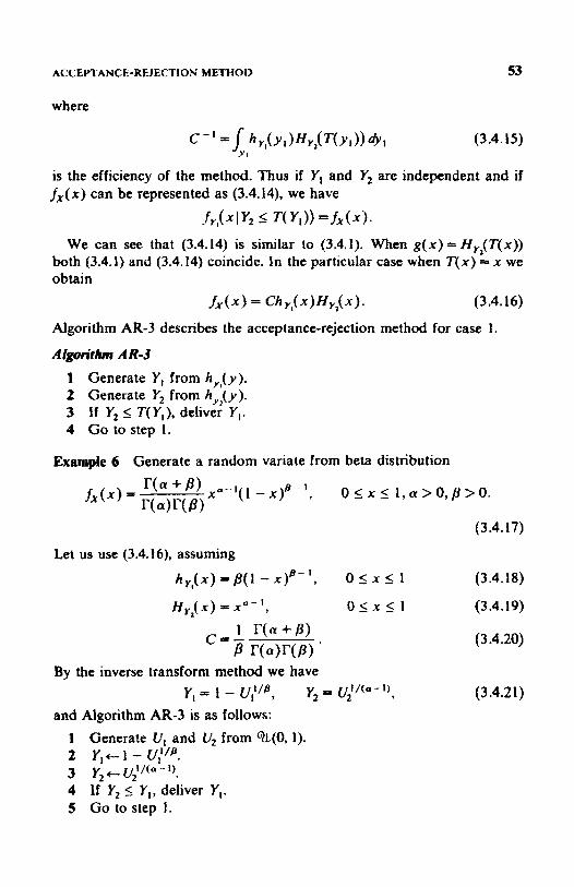
ACCEPTANCE-REJECTION METHOI) 53
where
c - ' = / h , I ( Y , W , j T ( Y , ) ) d L , (3.4.15)
is the efficiency of the method. Thus if Y, and Yz are independent and if f x ( x ) can be represented as (3.4,14), we have
Y I
f Y f . d Y 2 -< T( Y,)) = f x ( x ) .
We can see that (3.4.14) is similar to (3.4.1). When g ( x ) = H,,(T(x)) both (3.4.1) and (3.4.14) coincide. In the particular case when T ( x ) = x we obtain
f x ( x ) = Ch,,(xW,jx). (3.4.16)
Algorithm AR-3 describes the acceptance-rejection method for case I.
Atgoritkm AR-3 1 Generate Y, from h,,,(y). 2 Generate Yz from h,,,(y). 3 If Y2 5 T(Y,) , deliver Y,. 4 Go to step 1.
Example 6 Generate a random variate from beta distribution
(3.4.17)
Let us use (3.4.16), assuming
h y , ( X ) - /3(1- x ) P - l , 0 I x 2 1 (3.4.18)
H , j x ) = x u - I , 0 5 X l l (3.4.19)
(3.4.20)
By the inverse transform method we have Y , = 1 - u y ,
and Algorithm AR-3 is as follows:
Y, * u. I/(" - I t (3.4.2 1)
1 Generate U, and U2 from %.(O, 1). 2 Y , c 1 - u y . 3 Y 2 t . U p - ' f . 4 If Yz 5 Y,, deliver Y,. 5 Go to step 1.

54 RANDOM VARIATE OENERATION
Example 7 Consider again the problem of generating a random variate from beta distribution (3.4.17). Let us make use of (3.4.14), assuming
h,I(x) = axa-" , O l x l l (3.4.22)
(3.4.23) H , j T ( x ) ) = ( 1 - x)@- 1, 0 I x I 1
(3.4.24)
(3.4.25)
By the inverse transform method Y, = U;/a, Y, = Ui/(@-'), and Algorithm AR-3 is as follows:
1 Generate U, and U, from Gz.(O, 1). 2 Y , c u y . 3 Y 2 c up(@- 1).
4 5 Go to step 1.
If Y2 I. 1 - Y,, deliver Y,.
Remark If f x ( x ) can be represented as f x ( x ) = Ch,,(xNl - H,JT(x))] , then it is easy to see that Algorithm AR-3 can be written as follows.
A l g o ~ t h AR-3' I Generate Y, from hy, (y ) . 2 Generate Y, from h,l(y). 3 If Y, 2 T( Y,), deliver Y,. 4 Go to step 1.
CASE 2 Let 0 5 T ( x ) 5 M and let Y2 be from qL(0, M), that is,
I (3.4.26) 0 l Y , 5 M
h y $ Y 2 ) = M' 1, otherwise. Then i t follows directly from (3.4.13) that
(3.4.27) h Y , ( x )I'( x ?
f a x ) = = C,h, , (x)T(x) ,
where

ACCEPTANCE-RFJECTION METHOD 55
The efficiency of the method is
(3.4.29)
Substituting C , = C/M in (3.4.1) and denoting g(x) = T ( x ) / M , we obtain = ChY,(XMXh (3.4.30)
which is exacdy (3.4.1). So case 2 corresponds to Algorithm AR-I.
Example 8 Consider again the problem of generating a random variate from beta distribution (3.4.17), representing f x ( x ) as in (3.4.30), that is, applying Aigorithm AR-1 and taking into account that
g( x) = HY,(X) = xu- (3.4.3.1)
and
g ( x ) = H , j T ( x ) ) = (1 - x Y - I, (3.4.32)
respectively, for both examples 6 and 7; Algorithm AR-1 for example 6 (see (3.4.17) through (3.4.21)) can be written as:
1 Generate U, and U, from %(O, 1).
3 i f U, 5 Y O - ' , deliver Y. 4 Go to step 1.
2 Y t 1 - u;'?
Similarly, for example 7 Algorithm AR-I can be written as: 1 Generate LI, and Uz from %(O, I). 2 y c u ; / = . 3 If U, I ( I - Y ) @ - ' , deliver Y. 4 Go to step 1.
CASE 3 Let u I x 5 b, 0 5 7(x) 5 M, and let Y, and Yz be independent r.v.'s distributed %,(a. 6) and %(O, M), respectively. We immediately ob- tain from (3.4.14)
fA-4 = Tfx). (3.4.33)
Rewritingf'(x) in the standard way (3.4.1)
= C h ( x ) g ( x ) ,
56
we have
RANDOM VARIATE GENERATION
C = M ( b - a ) (3.4.34)
a l x l b
otherwise
1 (3.4.35)
(3.4.36)
Therefore case 3 corresponds to Algorithm AR-2.
We can easily see that Algorithm AR-3 generalizes both Algorithms AR-I and AR-2 in the sense that, when h,l(x) is distributed uniformly, we obtain Algorithm AR-I, and when both h,l(x) and h,$x) are distributed uniformly, we obtain Algorithm AR-2. But (3.4.1) generalizes (3.4.14) in the sense that the c.d.f. HyJT(x)) is a particular case of g(x), 0 I g(x) < 1.
RESUME: Formula (3.4.1) generalizes 3.4.14. In the particular case when g ( x ) can be represented as a c.d.f. H,t(T(x)) from which a random variate Yz can be easiiy generated, Algorithm AR-3 generalizes Algo- rithm AR-I and as a rule saves computation (CPU) time.
Formula (3.4.14) can be extended easily for the multivariate case.
Theorem 3.43 Let Y = (Y,, . . . , Y,,) be a random vector with p.d.f. h, (x ) , x=(x,, . ..,x,,), and let W be a random variable with p.d.f. h,(w), w E [ O , MI. Let T ( x ) be an arbitrary continuous function such that sup, T ( x ) = M. Then
fy, I . . . 9 y, ( X I , . . . , x, 1 w 5 T( Y )) = Ch ,( x)H, ( T( x)), (3.4.37)
where
The proof of this theorem is left for the reader.
3.4.4 Forsythe’s Method
Forsythe’s method is a rejection technique for sampling from a continu- ous distribution. The original idea is attributed to von Neumann [34]. Forsythe [ 151 described the method explicitly. Other descriptions are given by Ahrens and Dieter [2] and Fishman [ 121 with an application to different distributions. Our nomenclature follows that of Forsythe.

ACCEIYTANCE-REJECTION METHOD 57
Suppose we wish to generate a random variable X from any p.d.f. of the form
where
(3.4.39)
and h ( x ) is an increasing function of x over the range [0, 001. In the first stage of the method an interval is selected for x, and in the second stage the value of x is determined within the interval by a rejection.
For each k = 1,2,. . . , K (K is defined below} pick g, as large as possible subject to the constraints
Next compute h ( g k ) - h ( g k - l ) 5 1, g,=O- (3.4.40)
r, = i g k j x ( x ) c i x , /c = 1,. . . ,K. (3.4.4 I )
Here the number of intervals, K, is chosen as the least index such that r, exceeds the largest number less than one that can be represented in a computer. ( K may be chosen smaller if we set f k = i , and if we are willing to truncate the generated variable by reducing any value above gk to the interval I&-, ,&). Finally, compute
d k = g k - g k - , . k = 1, ..., K (3.4.42)
and the function
Gk( X ) = h( g, - 1 -t X ) - h( gk - i ) 5 h (gi ) - h( gk - ) 5 1 3 0 5 X 5 dk . (3.4.43)
Now we present the algorithm. Steps I to 3 determine which interval [gk- , .gk ) the variabley will belong to. Steps 4 to 8 determine the value of y within that interval.
AIgorirkm F- I 1 Set k c 1. Generate U fram 9L(4 1). 2 If U 5 r,, go to step 4 (the k th interval is selected). 3 If U > r,, set k t k + I and go back to step I . 4 Generate another uniform deviate U and set X = Ud,. 5 S e t t + G , ( X ) . 6 Generate U,, U,, . . . , U, where N is such that r > U,, t > U., ..., I >
7 If N is even, reject X and return to step 1. 8 If N is odd, accept X.
U,- I , but t I V, (N = 1 if 1 I Ui).
s8 RANDOM VARIATE GENERATION
The proof of the method is given in Forsythe [I51 (see also Fishman [12, p. 4001 and Ahrens and Dieter [2]).
Example 1 For h ( x ) = x, f x ( x ) is a standard exponential distribution and we have g, = k , d, = 1, and r, = 1 - e - k for all k.
Exponentid Distribution
Example 2 Normal Distribution For h ( x ) = x2/2, f x ( x ) corresponds to the positive half of the normal distribution and we have go = 0, g, = 1,
3)’/’, and k 2 2. Also g, = (2k - k 2 2. d , = 1, d , = 3”’ - I , . . . , d , = (2k - 1)”’ - (2k -
X 2 G , ( x ) = ~ + g , - i ~ , k L 1-
The advantage of this method is that it provides a rejection technique for densities of the form (3.4.39) without the need for exponentiation. If G,( x) is easier to calculate than e - h ( x ? as it is for many members of the exponential family, the method can yield fast algorithms.
An important feature of the method is that it does not specify a unique algorithm, but rather a family of algorithms, subject to (3.4.40) being satisfied. The interval widths d, can be chosen at will.
A disadvantage of the method is that it requires tables of the constants g&, d&v and rk.
3.5 S I M U T I O N OF RANDOM VECTORS
35.1 loverse Transform Method
c.d.f. F,(x). We distinguish the following two cases. Let X = (X,, . . . , X,,) be a random vector to be generated from the given
CASE 1 joint p.d.f. is
The random variables XI.. . . , A’,, are independent. In this case the
n
f x ,...., x , ( h .. - 4) - II f ; ( x , ) * (3.5.1)
whereJ(xi) Is the marginal p.d.f. of the random variable Xi. It is easy to see that, in order to generate the random vector X =(XI,, . . , X , ) from c.d.f. Fx(x) , we can apply the inverse-transform method
X, = &-‘(q) , i== 1 ,..., n (3 5 2 )
1 - 1
to each variable separately.

SIMULATION OF RANDOM VECTORS 59
Exsmple 1 Let XI be independent r.v.'s with the p.d.f.
I 1 1 - - , a , < x , < h , , i = i ,..., n
\O, otherwise. To generate the random vector X = (XI, . . . , X, , ) with the joint p.d.f.
f ; (X , ) = b, - a ,
1 I (xI, . . . , x , , ) E D
-ti, , , , , x j x I . . . . * x n ) = 1 il ( b t - a , )
lo.-' otherwise
where D = (xi , . . . , x n ) : a , 5 x, 5 b,, i = I , . . . . n } , we apply the inverse transform formula (3.5.2) and get X, = a, + (b, - u,)V, i = 1,. . . , P I .
CASE 2 The random variables are dependent. In this case the joint c.d.f. is
Tbeorem 3.5.1 Let U , . . . . , Un be independent uniformly distributed ran- dom variates from %(O. 1). Then the vector X = ( X I , . .. ,A',), which is obtained from the solution o f the following system of equations
FAXI) = u,
(3.5.4)
is distributed according ta cv(.xj. The proof of this theorem is similar to the proof of (3.2.2) and is left for the reader.
The procedure for generating random variates from (3.5.3) contains only two steps.
I Generate n independent uniformly distributed variates from %(O, 1). 2 Solve the system of equations (3.5.4) with respect to X = ( X I , . . . , X,,).
There are n ! ordered combinations (possibilities) to represent the varia- bles X I , . . . , Xn in vector X , and therefore n! possibilities to generate X while solving (3.5.4). Thus for n = 2 and n! = 2 we can write fx,,x,(xl, x 2 )

60 RANWM VARIATE GENERATION
in two different ways:
(3.5.5)
(3.5.6)
The efficiency of simulation will generally depend on the order in which the random variates X i , i = 1,. . . , n , are taken while forming the random vector X.
The following example, which is taken from Sobol [29], uses both formulas (3.5.5) and (3.5.6) for generating a two-variate random vector X = (XI, X 2 ) and shows the difference in their efficiency.
Example 1
if x, + x2 I 1, x1 10.~2 2 0 fX,,X,(x17x2) = { otherwise.
CASE 1
fx, , * , (x 1 x2 = f,( X l Mi( x2 I x , 1. The marginal p.d.f. of the r.v. XI is
ft(x1) =i'-+ f x , x , ( x , , x ~ ) ~ x ~ = ~ x , ( ~ -xI ) , 0 < x l I I .
The conditional p.d.f. of the r.v. X, , gwen XI = xl, is
The correspondent marginal and conditional distribution functions are, respectively,
CASE 2

SIMULATKON OF RANDOM vEcrms 61
The corresponding marginal and conditional distribution functions are
Fl( x , I x 2 ) = J”), ( x , I X I ) dr , = x f ( 1 - x2) - z, 0 I x , I I - x2 0
and the system (3.5.4) is 1 - (1 - X 2 ) ] = u, i Xf( l -x2)-2=u2
i x; = U2( 1 - X$.
Inasmuch as I - U is distributed in the same way as U, the last system can be written
( I --x,)’= u1
Comparing both cases, we can see that the first system is rather difficult to solve (we would have to solve cubic and quadratic equations, respectively), while the second system has a trivial soIution
x, = 1 - uy3
x, = u y w y . Unfortunately, there is no way to find a priori the optimal order of representing the variates in the vector to minimize the CPU time.
Remark For independent r.v.’s the efficiency of simulation does not depend on the order in which the r.v.’s are taken in forming the random vector X.
An alternative method for generating random vectors is the acceptance- rejection method based on Theorem 3.4.3.
35.2 Multivariate Transformation Metbod
This method can sometimes be useful for generating both random variables and random vectors.

62 RANDOM VARlATE GENERATION
Suppose that we are given the joint p.d.f. fx ,,.-., xJxI ,..., xn) of the n-dimensional continuous random variable (XI, . . . , Xm). Let
K' { (X I , . . . . X n ) :fx,... . x l X l * . . . , X , ) > 0) - (3.5.7)
Again assume that the joint density of the random variables Y, = g, (X, , . . . ,A',), . . . , Y, = gk( X i , . . . ,X , , ) is desired, where k is an integer satisfying 1 I k I n. If k < n, we introduce additional new random varia- bles Y k + , = g k + , ( X i , . . . , X,,), . . . , Y,, = g, (X, , . . . ,A',,) for judiciously selected functions g , , I , . . . ,g,,; then we find the joint distribution of Y, ,..., Y,; finally, we find the desired marginal distribution of Y ,,..., Y, from the joint distribution of Y,, . . . , Y,. This use of possibly introducing additional random variables makes the transformation y , = g , ( x , , . . . , x J r . . . ,y,, = g,(xl, . . . , x") a transformation from an n- dimensional space to an n-dimensional space. Henceforth we assume that we are seeking the joint distribution of Y, = g , ( X , , . . .,A',), . . ., Y, - g , ( X , , . . . , X,,) (rather than the joint distribution of Y , , . . . , Y,) when we have given the joint probability density of Xi,, . . , X,,.
We state our results for n = 2. The generalization for n > 2 is straightfor- ward. Let fx , , , , (x , ,x , ) be given. Set K = {(x1.x2) : fx , .x , (x1 .x2) > 0). We want to find the joint distribution of Y, = gl( XI, X,) and Y, = g , ( X , , X,) for known functions g,(x,,x,) and g 2 ( x , . x 2 ) . Now suppose that y I = g,(x,, x , ) and yz 5 g 2 ( x I , x,) defines ;t one-to-one transformation that maps K onto, say, D. x , and x 2 can be expressed in terms of yl and y2; so we can write, say. x , = 'pI ( y , , y 2 ) and x2 = tp2 (y1,y2). Note that K is a subset of the xIx2 plane and D is a subset of theyly2 plane consisting of points ( y l , y 2 ) for which there exist a ( x , , x , ) E ~ such that ( y l , y 2 ) = [gl(xI,x2), g2(x,,x2)]. The determinant
is called the Jacobian of the transformation and is denoted by J . The above discussion permits us to stale Theorem 3.5.2.
Theorem 3.52 Let Xi and X , be jointly continuous random variables with density function f x , , x , ( x , , x 2 ) . Set K = { ( x I , x 2 ) : fx , , x ,Cx l ,x z ) > 0) . Assume that:
1 y , =gl(x,,x2) and y , =g2(xl,x2) defines a one-to-one transforma- tion of K onto D.

SIMULATION OF RANDOM VECTORS 63
2 The first partial derivatives of x , = q,(y1,y2) and x2 = (p2(y,,y2) are
3 The Jacobian of the transformation is nonzero for (yI,y2) E D. Then continuous over D .
the joint density of Y, = gt( XI, X,) and Y, = g2( XI, X 2 ) is given by f,,, Y,< Y I 9Y2 = I J 1 fx,, x,( Q I( Yl 9Y2 ) 9 d Y t PY2 ) ) I D ( Yl rY2 ). (3 -5.8)
where
The proof is essentially the derivation of the formulas for transforming variables in double integrals. For proof, the reader is referred to Neuts ~ 5 1 .
For the single variate case the transformation formula (3.5.8) becomes
(3.5.9)
Heref,(x) is the given p.d.f.,fy(y) is the desired p.d.f., 1, is the interval of x, and Y PL: g( X ). We can see that (3.5.9) is a particular case of (3.5.8).
Example I variables. Let Y, = Z , + Z2 and Y2 = Z, /Z2 . Then
Let Z, and Z2 be two independent standard normal random
Y2 1 +Y2
I J =
I I + Y 2
Y l
( 1 + Y d 2
To find the marginal distribution of, say Y,, we must integrate out yl, that
64
is
R A h W M VARIATE GENERATION
Let
then
and so
a Cauchy density. In other words, the ratio of two independent standard normal random variables has 3 Cauchy distribution.
To generate an r.v. from a Cauchy distribution we generate Z, and Z2 from N(0, 1) and take their ratio.
Example 2 Let Xi have a gamma distribution
x , 2 0, n i > O 0, otherwise
with parameters ni and I for i = 1,2, and assume X , and X2 are indepen- dent. Suppose now that the distribution of Y, = X , / ( X , + X,) is desired. We have only the one function y , = gI(xI,x2) = x1 /(x, + x2), so we have to select the other to use the transformation technique. Since x , and x2 occur in the exponent of their joint density as their sum, x , + x2 is a good choice. Let y2 = x , + x2; then xi = y l y 2 , x2 =y2 - y,y2, and
J = l Y2 I - Y , y' I'Y2. - Y2

SIMULATION OF RANDOM VECTORS 65
Hence
It turns out that Yl and Yz are independent and that Y, has a beta distribution with parameters n l and n2.
Thus to generate a random variate from beta distribution we generate two gamma variates X , and X 2 , then calculate Xl/(Xl + X2) .
3.5.3 Muitinormal Distribution
p.d.f. is given by A random vector X = (X,. . . . , X n ) has a multinormal distribution if the
exp[ - f ( x - p ) 7 X c - 1 ( x - p)] (3.5.10) I f x ( x ) =
(27r)n'2p(
and denoted by N(p. C).
matrix Here p = (pl.. . . . p n ) is the mean vector, I: is the covariance ( n X n)
'72 n
which is positive definite and symmetric, 1x1 is the determinant of 2, and I: I is the inverse matrix of I:.
Inasmuch as C is positive definite and symmetric, there exists a unique lower triangular matrix
CI1 0 - * - 0 0 . . . c21 c22 C = (3 -5.12)

66 RANDOM VARIATE GENERATION
such that
z = CCT. (3.5.13)
Then the vector X can be represented as x==cz+p, (3.5.14)
where Z = (Z,, . . . , Z,) is a normal vector with zero mean and covariance matrix equal to identity matrix, that is, all components Z,, i = 1,. . . , n, of 2 are distributed according to the standard normal distribution N(0, 1 ).
In order to obtain C from C = CC’ the so-called “square root method” can be used, which provides a set of recursive formulas for computation of the elements of C.
It follows from (3.5.14) that
X,=c,,Z,+I.r , . (3.5.15)
Therefore var X I = u , ~ = obtain
and c, I = u:(‘. Proceeding with (3.5.14) we
(3.5.16) x, = C 2 I G + c222 + P 2
and var X, = u2, = var( cZ1Z, + c2*Z2). (3.5.17)
From (3.5.15) and (3.5.16)
E[W, - - P , ) ( - Y , - P d I = 0 1 2 = ~ [ c l l ~ l ( C 2 I Z I + C 2 2 Z 2 ) ] . (33.18)
From (3.5.17) and (3.5.18)
(3.5.19)
(3.5.20)
Generally, c , ~ can be found from the following recursive formula: J - 1
- 2 C,kCjk k = I
c,, = (3.5.2 1) J - 1 I / , ’ ( ‘JJ - ‘;k)
where

GENERATING FROM CONTINUOUS DISTRIBUTIONS 67
Algorithm MN-I describes the necessary steps for generating a muitinor- ma1 variate.
Aigon3h MN-1
1
where
2 Generate Z = (Z , , . . . , 2,) from N ( 0 , 1).
4 Deliver X. 3 X t C Z + p .
3.6 GENERATING FROM CONTINUOUS DISTRIBUTIONS
This section describes generating procedures for various single-variate continuous distributions.
3.6.1 Exponential Distribution
An exponential variate X has p.d.f.
(3.6.1) otherwise
denoted by exp(p).
Pmcedune E- I By inverse transform method
u = ~ ~ ( x ) = 1 -e-.' 'fl (3.6.2) so that
X = -[3ln(l - U ) . (3.6.3)
Since I - U is distributed in the same way as U, we have X = -p ln U . (3.6.4)

68 RANDOM VAIUATE GENERATION
For sampiing purposes we may assume /3 = I : if Y is sampled from the standard exponential distribution exp( I), then X = PV is from exp(P).
Algorithm E-1 1 Generate U from %(O, I). 2 X t - B l n l J . 3 Deliver X .
Although this technique seems very simple, the computation of the natural logarithm on a digital computer includes a power series expansion (or some equivalent approximation technique) for each uniform variate gener- ated.
P m d a E-2 We now prove a proposition that can be useful for generating from exponential distribution exp( 1).
Proposition Let U , , , . . , V,, U n + l , . . .. U2,-, be independent uniformly distributed random variables, and let YIt , . . . , L&,- ,) represent the order statistics corresponding to the random sample U,, . . , U2"- I. Assume U,, = 0 and Ute, = I ; then the r.v.'s
n
Y& = (q,. I ) - q,,)in n o,, k = 1. ..., n (3.6.5) I - I
are independent and distributed exp( 1).
Proof Denote
X , - qL)-- q k -,,, k = 1 ,..-, n - 1
and n
x,= - I n n v , . It will be shown in Section 3.6.2 that X, is from the Erlang distribution, that is,
1 - 1
(3.6.6)
It is aiso known (Feller [ I I]) that the vector ( X , , . . . ,Xn- ,) is distributed fx ,,..., X a . I ( ~ 1 ~ * * * r x n - 1 ) ~ ( n - I ) ! (3.6.7)
inside the simplex n- I ~ x x , s l , x ,20, k = l , . . - , n - I .
k - I

GENERATING FROM CONTINUOUS DISTRIBUTIONS 69
Hence
Iv , , . , . , YJY I -
n
= I l e - * < , ~ , ~ o , i - - i ,.... n . (3.6.9)
Q.E.D. I - I
For n = 3 we have
1 3 \

70 RANDOM VARIATE GENERATION
Algorithm E-2 describes the necessary steps.
Alpt i thm E- 2
1 Generate 2n - 1 uniformly distributed random variates U,, . . . , 2 Arrange the variates U,, ,, . . . , U2,,- , in order of increasing ma@-
u,, u,, ,, . - ., UZn- 1’
tudes, that is, define them to be the order statistics q,,, . . . , q,,- ,). 3 Y k t ( q k - 1 ) - qk))ln(n;-&(h k = l , * . * , n * 4 Deliver Y,, k = 1,. . . , n, as an r.v. from exp(1).
Comparing (3.6.5) with the inverse transform method Y,= -In&, k = l , ..., n,
we find that the advantage of Algorithm E-2 is that it requires only one computation of In n;,,U, for generating n exponential variates simulta- neously. In the same time the inverse transform method requires n compu- tations of In u k for each variate Y,, k = 1, .. . ,n, separately. The disadvantage of Algorithm E-2 is that it needs 2n- I uniform variates rather than n uniform variates for the inverse transform method. Addition- ally, Algorithm E-2 requires the arrangement of the uniform variates CJ, ,+ , , . . .. to be order statistics U(i), . . ., if(,,-.,) and then calculation of U(k- ,) - q k ) , which is also time consuming.
Simulating both algorithms we find that Algonthm E-2 is faster than the standard inverse Algorithm E-I for n = 3 to n = 6. The optimal n is 4.
There are many alternative procedures (Ahrens and Dieter [ 11, Marsaglia [19]) for generating from exp(8) without the benefit of a logarithmic transformation, procedures that are based on the composition method, acceptance-rejection method, and Forsythe method [IS] (see also example 1, Section 3.4.4). The reader is also referred to Fishman’s monograph [ 121. Before leaving the exponential distribution we want to introduce von Neumann’s ingenious method [34] for generating from exp(l), a method that was later extended by Forsythe (151 and Ahrens and Dieter [2] for generating various distributions.
Let ( X , : i = 0, . . . } be a sequence of i.1.d. r.v.’s from the standard triangular distribution
and define an r.v. N, taking positive integer values through ( X i } by the

GENERATlNG FROM CONTlNUOUS DISTRIBUTIONS 71
inequaii ties 2 N- I I4
x , 5 x o , C X J l X 0 ”.., X J S X ~ . ~ x , > X , . 1- 1 J v l 1-1
We accept the sequence { X,} if N is odd; otherwise we reject it and repeat the process until N turns out odd. Let T be the number of sequences rejected before an odd N appears (T = 0.1, . . . ) and let X, be the value of the first variable in the accepted sequence; then Y = T + Xo is from exp(1). It is shown in ref. 34 that generation of one exponentional variate in such a way requires on the average (1 + e ) (1 - e - ’1 = 6 random numbers.
3.6.2 Ganuna Distribution
A random variable X has a gamma distribution if its p.d.f. is defined as
otherwise,
and is denoted by G(a,P). Note that for (x = I, C(1,p) is exp(P). Inasmuch as the c.d.f. does not exist in explicit form for gamma
distribution, the inverse transform method cannot be applied. Therefore alternative methods of generating gamma variates must be considered.
k e d m G-1
One of the most important properties of gamma distribution is the repro- ductive property, which can be successfully used for gamma generation. Let Xi, i = 1,. . . , n, be a sequence of independent random variables from G( ai, 8). Then X = Xy-, X, is from G( a, 0) where a = Xy- pi.
If a is an integer, say, a = m, a random variate from gamma distribution G(rn,/I) can be obtained by summing m independent exponentiaf random variates exp( p), that is,
m m
X - P ~ (--InU,)== -pin I1 u,, i= I i.; I
which is called Erlang distribution and denoted Er(m, p). describes generating r.v.’s from Er(m, p). A l g ~ t i t b i G-1
1 X t O . 2 Generate V from expfl). 3 X t X + Y .
(3.6.10)
Algorithm G-1
72 RANDOM VARIATE GENERATION
4 5 ata-I. 6 Go to step 2.
It is not difficult to see that the mean computation (CPU) time for generation from Erlang distribution is an increasing linear function of a. However, if a is nonintegral, (3.6.10) is not applicable and some difficulties arise while generating gamma variates.
For some time no exact method was known and approximate techniques were used. The most common method was the so-called probability switch method [24].
Let m = [a] be the integral part of a and let 6 = a - m. With probability 6, generate a random variate from Gfm + l ,@). With probability I - 6, generate a random variate from G( m, /I). This mixture of gamma variates with integral shape parameters will approximate the desired gamma distri- bution. This technique will only work when a 2 1.
In the particular case when a=; gamma variables can be generated exactly by adding half the square of a standard normal variate to the variate generated in (3.6.10).
Proc4drcrp G-2
Johnk [ 161 suggested a technique that exactly generates' variates from G ( 6 , P ) , where O < 6 < 1.
If a = 1, X C ~ X and deliver X.
Theorem 3.6.1 Let W and V be independent variates from beta distri- bution Be(& 1 - 6) (see Section 3.6.3) and exp(l), respectively. Then X = /3V W is a variate with G( 6, li).
Prmf of this transformation is
Let u = v and let x = @w. Then w = x /@u, and v = u. The Jacobian
(3.6.1 1)
The joint distribution of ( u , x) is therefore given by
otherwise. (3.6.12)
*It is understood that when we say a method "exactly generates" random variables on a computer, that the exactness is limited by the computer used and by the randomness of the underlying pseudorandom number generator.

GENERATING FROM CON I'INUOUS DISTRIBUTIONS 73
The marginal distribution for X is
which is G(S, p). Q.E.D. A I & t h C-2
I Generate two variates W and Y from Be(& I - 6) and exp(l),
2 Compute X = pYW that is from G(S,B). 3. Deliver A'.
respectively.
To generate a variate from G((w,P) we generate an r.v. Y from Er(rn, l), then compute X = p( Y+ V W ) , which is from G ( a , P ) . Here IY = 6 + m.
Recently, a number of procedures for sampling from G(a,B), based on the acceptance-rejection method, were suggested by Ahrens and Dieter [3], Cheng [9], Fishman [13), Tadikamalla [30, 311 and Wallace [35]. Let us consider some of them.
Procedure c-3 Wallace [35] suggested a procedure for generating from G(a, 1) with a > 1 based on both the acceptance-rejection and probability switch methods.
Let
f.(.) = C h ( X k ( X ) P
where h ( x ) is a mixture of two Erlang distributions Er(m, I ) and E r ( m + I , 1) equal to
x"'e-" X m - l - -x e h ( x ) = P + ( I - P)-- x 2 0, (3.6.13) ( m - l ) ! m ! '
and
g ( + 4 = ( ; ) u [ I + ( < - m $1
(3.6.14)
(3.6.15)
It can be found from (3.4.10) that the optimal P is equal to I - 6, where 6 = a - [a]. I t follows from (3.6.14) that the mean number of trials C is a monotone decreasing function of rn for a fixed S and
(m - l ) ! d lim = I ,
m+oo r ( m + 8 )

74 RANDOM VARIATE GENERATJON
that is, asymptotically the execution time does not depend on S and achieves optimal efficiency C = 1. Algorithm G-3 describes Wallace's procedure.
Al-*thm G-3 1 Compute 6 = a - m, where m = [a]. 2 Generate Cr ,,.. ., U, from %(O, I). 3 With probability 1 - 6 compute
rn
v- -In 11 q. i- I
4 With probability 6 compute m+ I
v = - I ~ u,. i= 1
5 Generate another uniform variate U from %(O, I). 6 If U I ( V / m ) ' / [ 1 + ( ( V ( / m ) - I)&], deliver V as an r.v. from G(a, 1). 7 Go to step 2.
The following three procedures are reproduced with little change from Ref. 12.
Proaedwe GC Fishman [13) describes another procedure for generating from G(a , l), a 2 I :
exp[ -X( I - ]/a)] (YO 'exp( 1 - a)
g(x) = x a - ' (3.6.16)
& ) = L , - X / . a (3.6.17)
The probability of success on a trial is
1 c aaeI-o ' -=-
For large a the mean number of trials is
(3.6.18)
(3.6.19)
(3 A.20)
It is not difficult to see that the condition U 5 g ( Y ) , where the r.v. Y is

GENERATING FROM CONTINUOUS nISTRIBUTtONS 75
from exp(l/a), can be written as V, 2 f a - 1)( V, - In V, - 1) and V, and V2 are independent r.v.’s from exp(1).
Algoritlun G-4 1 A c a - 1 . 2 Generate V, and V2 from exp(1). 3 If Vz < A(V, - In V, - I ) , go to step 2. 4 Deliver V, as a variate from G(a, I).
Pmcedum G-5 This procedure is due to Cheng 191 and describes gamma generation G(a , 1) for a > 1 with execution time asymptotically independent of a.
In Cheng’s procedure
* ( p + x ” - 2 , x 2 0 (3.6.2 1 ) otherwise
h ( x ) =
4a” c= r( a)eaX
ea-r g ( x ) = x a - A ( y + 2))’- 4*a+h ’
(3.6.22)
(3.6.23)
where
p 51 aAr A = (2a - The execution time C is a monotonicalty decreasing function of a such that, for a = I, C = 1.47, and for a = 2, C = 1.25; asymptotically
2 lim C=-m 1.13. p4ao G
(3 -6.24)
Let b = a - In 4 and d = a + l / X . Then Cheng’s algorithm can be writ- ten as follows.
A f g d h G-5 1 Sample U, and U2 from %(O, I ) . 2 Vc-X In[U, /( 1 - &)I. 3 X c a e ’ . 4 If b + d - X 2 ln(U,2V2), deliver X. 5 Go to step I .
P h ~ b G-6 Ahrens and Dieter [3] suggested an alternative procedure for generating from G(a ,p ) with a > 1 and execution time independent of a asymptoti-
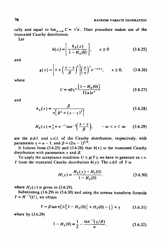
76 RANDOM VAIUATE GENERATION
cally and equal to lima-ta C = L/m. Their procedure makes use of the truncated Cauchy distribution.
Let
(3.6.25)
and
where
and
(3.6.27)
(3.6.28)
H , ( x ) = 1 + tan-'( 7 ), - 00 < x < 00 (3.6.29)
are the p.d.f. and c.d.f. of the Cauchy distribution, respectively, with parameters y = a - 1. and p = (2a - 1)'/2.
I t follows from (3.6.25) and (3.6.28) that h ( x ) is the truncated Cauchy distribution with parameters y and p.
To apply the acceptance condition U 5 g( Y ), we have to generate an r.v. Y from the truncated Cauchy distribution h ( y ) . The c.d.f. of Y is
(3.6 -30)
where H , ( y ) is given in (3.6.29).
Y = H - ' ( U ) , we obtain Substituting (3.6.29) in (3.6.30) and using the inverse transform formula
Y-ptanTr(u[I - H , ( o ) ] + H , ( o ) - ~ } + y (3.6.3 1)
where by (3.6.29)
(3.6.32)

OENERATING FROM CONTINUOUS DISTRIBUTIONS 77
It is readily seen that the condition U 5 g ( Y ) is equivalent to
y' - V = I n U < h g ( Y ) = i n [ 1 + ( y i 2 y ) 2 ] + y l n T - r+y, (3.6.33)
where I/ is from exp(1). Y' = y + p tans(U -;) and can be found from u = Hy(y). A f @ t h G-6
1 yea-1. 2 Generate U from %(O, 1). 3 ~ ' t - y + tans(U - f 1. 4 Generate V from exp(1). 5 6 Go to step 2.
The following two procedures for generating from C(a , 1) are due to Tadikamalla [30, 311.
If - V I In[ 1 + (Y' - y)2 / /?2 ] + y In( Y ' / y ) - Y' + y , deliver Y'.
P * o c t d ~ ~ 6 - 7
In this procedure 1301 h ( x ) is froin Er(m,p) , that is,
Then it is readily shown that xsexp[ -X(I - I/P)]
g ( x ) = , X L O (3.6.35) [ s p / ( p - - 1 ) ] % - *
(3.6.36)
where 6 = a - m and m = [a]. The value of a that maximizes the efficiency can be found from (3.4.10)
and is equal to a/m. Tadikamalla showed by simulation that his procedure is faster than
Fishman's Procedure G-4 for 3 5 a I 19 and is comparable for other values of a. For 1 5 a < 2 both methods coincide. This is not surprising. The reason for the great efficiency of this procedure is that Erlang distribution Er(m, p), with n = [a], approximates the gamma distribution C( a, p ) better than the exponential distribution exp(a) (see Procedure G-4) does.

78 RANDOM VARIATE GENERATION
In addition, Tadikamalla's procedure is better than Ahrens and Dieter's Procedure G-6 for a S 8.
Algorihm G7 1 Compute &+a - m, where m = [a]. 2 Generate m independent random variates U,, . . . , Urn from %(O, 1). 3 Compute Y = -/3Inn;,q.. 4 Generate another uniform variate U from %(O, 1). 5 If
YGexp[ - ~ ( 1 - I/P)] U S
[ &I6e-6 '
deliver Y. 6 Go tostep2.
P m d W e G-8
In this procedure 1311 h ( x ) is from the Laplace (double exponential) distribution with location parameter a - I and scale parameter 8, that is,
Then it
(3.6.37)
is readily shown that
(3.6.38)
and
A I W * t h G-8 1 Generate a random vanate Y from the Laplace distribution with
2 If Y < 0, go to step 1. 3 Generate a uniform random variate from SL(0, 1). 4 If U I g( Y ) (see (3.6.38)), deliver X. 5 Go to step i .
Iocation parameter a - 1 and scale parameter 8.

GENERATLNG FROM COKFINUOCS D i s r m u r I o N s 79
Table 3.6.1 The Relative EXkkndes (l/C), and the Average Number of Roodom Numbers Required ( N ) for Certain Algorithms
Fishrnan Tadikamalla I Tadikamalla 2
a 1/c N 1/c N I/C N 1.5 0.7953 2.5 0.7953 2.5 0.8642 2.3 2.5 0.m9 3 -3 0.887 1 3.4 0.7872 2.5 3.5 0.5047 4 .O 0.9222 4.3 0.7565 2.6 5.5 0.3992 5 .O 0.9520 6.3 0.7304 2.7 8.5 0.3194 6.3 0.9695 9.3 0.7 174 2.8
10.5 0.2868 7 .O 0.9755 11.3 0.7144 2.8 15.5 0.2355 8.5 0.9836 16.3 0.7132 2.8 20.5 0.2045 9.8 0.9876 21.3 0.7 149 2.8 30.5 0.1674 11.9 0.9917 31.3 0.7 195 2.8
100.5 0.0920 21.7 I .oooo I01 .o 0.7355 2.7
Tadikamalla [31] compared the relative efficiency and CPU timing of his procedures with Fishman’s [13J and Ahrens and Dieter’s procedures [3].
Table 3.6.1 gives the relative efficiencies and the number of uniform random numbers required for these procedures for some selected values of a. The efficiencies of Ahrens and Dieter’s method are not given in Table 3.6.1 because these have to be calculated numerically and the details are not available in Ref. 3. For increasing values of a the efficiency of Fishman’s algorithm decreases and the efficiencies of Tadikamalla’s first algorithm (G-7) and of Ahrens and Dieter’s algorithm increase. The efficiency of ’Tadikamaila’s second algorithm (G-8) decreases as a in- creases up to a certain value and then it increases again. Also note that the number of uniforms required for Tadikamalla’s second algorithm (G-8) remains fairly constant.
Table 3.6.2 gives the CPU timings for these four methods on an IBM 370/165 computer, for selected values of a. These timings are based on generating 10,OOO variates and using the subroutine TIMER available on the IBM computer.
The following observations can be made about the methods compared above.
1 Fishman’s procedure is the simplest of all the procedures and the CPU time per trial is constant for any a. As a increases, the number of trials required for one gamma variate increases (efficiency decreases), and thus the CPU time per variate increases with a.
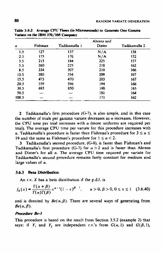
80 RANDOM VARIATE GENERATION
Table 3.63 Average CPU Times (in Micnxewh) to Generate One Gamma Varbte on the IBM 370/165 Computer
a Fishman Tadikamalla 1 Dieter Tadikamalla 2 Ahrens and
1.5 2.5 3.5 5.5 8.5
10.5 15.5 20.5 30.5 50.5 100.5
127 I75 213 260 334 380 473 559 693 -
I37 176 184 225 307 3 54 470 596 850 -
N/A N / A 225 218 2 10 209 203 1 94 190 181 171
138 152 157 I62 166 167 167 166 165 164 1 62
2 Tadikamalla’s first procedure (G-7), is also simple, and in this case the number of trials per gamma variate decreases as a increases. However, the CPU time per trial increases with a (more uniforms are required per trial). The average CPU time per variate for this procedure increases with a. Tadikamalla’s procedure is faster than Fishman’s procedure for 3 I a I 19 and the same as Fishman’s procedure for I 5 a < 2.
3 Tadikamalla’s second procedure, (G-8), is faster than Fishman’s and Tadikamalla’s first procedure (G-7) for a > 2 and is faster than Ahrens and Dieter’s fur all a. The average CPU time required per variate for Tadikamalla’s second procedure remains fairly constant for medium and large values of a.
3.63 Beta Distribution
An r.v. X has a beta distribution if the p.d.f. is
and is denoted by &(a,@). There are several ways of generating from Be(a, PI. Procedum &-I This procedure is based on the result from Section 3.5.2 (example 2) that says: if Y, and Yz are independent r.v.’s from G(a, 1) and G(P, l),

GENERATING FROM CONTINUOUS DISTRIBUTIONS 81
respectively, then
(3.6.4 1)
is from Be(a, p) . The corresponding algorithm is as follows.
Algoritkm Bp-1
1 Generate Yt from G(a, 1). 2 Generate Y2 form G(P, I ) , 3 4 Deliver X .
X t Y , / < Y, + Y2).
procrdurp Be- 2 Another approach when a and p are integers is based on the theory of order statistics. Let U,, . . , , be random variates from %(O, 1). Then the ath order statistic qat is from Be(a,#3). The algorithm is extremely simple.
Algorirhm Be- 2 1 Generate (a + #3 - 1) uniform random variates U , , . . . , Va+,-, from
2 Find U(a,, which is from Be(a,#3). %(O, 1).
It can be shown that the total number of comparisons needed to find qpt is equal to (a /2 ) ( a + 2p - I), that is, this procedure is not efficient for large a and 8.
Many procedures for sampling from Be( a, p ) with nonintegral a and p have been proposed recently (see Ahrens and Dieter (31, Cheng IS], Johnk [16], and Michailov [221). We consider only a few of them.
Procedure Be-3 The simplest procedure for generating from Be(a,B) with arbitrary nonin- tegral a and /3 uses the mode
(3.6.42)
which corresponds to x* - (a - I ) / ( a + p - 2).

82 RANDOM VARIATE GENERATION
The following algorithm, Be-3, is based on the acceptance-rejection Algorithm AR-2.
AIgM-thm Be-3 1
a - 1 + a - 2
2 Generate U, and U, from %(O, I). 3 If MU, 5 [T(a + p)/I'(a)I'(jI)]U?-'(l - U,)@-I, deliver U, as a
variate from Be( a, p).
procodrrne Be-4 This procedure is due to Jahnk 116) and is based on the following theorem.
4 Go to step 2.
Theorem 3.6.2 Let U, and U2 be two uniform vanates from %(O, 1) and let Y, = Uila and Y2 = fJ;'@. If Y, + Y, 5 1, then
is from B(a,/3).
Proof It is obvious that
f y , ( y , j = ayP- I. 0 iy, I 1
0 SYZ 5 1 J y J y 2 ) = / ? Y p i ,
and u - I 8-1
f Y , Y , ( Y , , Y 2 ) =aPYl Y2 *
Let X = Y, / ( Y l + Y,) and W = Y, + Yz. The Jacobian
(3.6.43)
(3.6.44)
(3.6.45)
(3.6.46)
=I 1-w (3.6.47) ax aw J = - - w I-x
ax a w

GENERATING FROM CONTINUOUS DiSrKlk3UTlONS 83
By Bayes' formula
(3.6.49)
Substituting (3.6:5 1 ) and (3.6.50) into (3.6.49), we obtain
Q.E.D. The efficiency of the method is equal to
(3.6.52) For integer a and P
(3.6.53)
Table 3.6.3 represents the mean number of trials C as a function of a and p. Asymptotically,
lim C - lirn C = lirn C = c o . 8;.0 U > O P-m u-rw &+m a-+m
Thus for large a or /3 Johnk's procedure is not efficient.
TaBie 3.63 I'be Mean Number of Trials as a Functlw of a and f i P
a I 3 1 2 4 6 3 4 20 56 5 6 56 252

84 RANDOM VARIATE GENERATION
Algorithm Be-4 1 j t l . 2 Generate V, and r/i+, from %(O, 1). 3 Y,+ u.''u. - , 4 Y2' q:/f. 5 If Yl + Y2 L 1, go to step 2. 6 j+-j+2. 7 Deliver X = Y, /( Y, + Y2).
P m e e h Be-5 This procedure is based on the results of examples 6 and 7 from Section 3.4.3. As follows from (3.4.20) and (3.4.24), the efficiencies of the accep- tance-rejection method AR-3 are, respectively,
in examples 6 and 7. For integer a and /? we have, respectively,
1 (a- I)!/?! c ( a + P - l ) ! I E --
I . ! ( P - I ) ! c (a+/?- I ) ! -=
(3.5.54)
(3.5.55)
(3.6.56)
(3.6.57)
In both cases (3.6.56) and (3.6.57) the efficiencies are a little higher than in Johnk's procedure Be4 (see (3.6.53)). I t is interesting to note that for p > a it is more efficient to represent J x ( x ) in the form of (3.4.18) through (3.4.20) and for a > /3 it is more efficient to representf,(x) in the form of (3.4.22) through (3.4.24).
Procediin? Be-6 In this procedure h ( x ) is Ee(m,n), that is,
( m + n - I ) ! (m- I ) ! (n - - I ) ! h ( x ) = x"-'(l - x y - I , 0 I x I 1
(3.6.58) where m = [ af and n = [ p]. Then

GENERATING FROM CONTINUOUS DlSTRIBUTIONS 85
where 6, = a - rn, S, = /3 - n, and B ( r , s ) = r ( r ) r ( s ) / I ' ( r + s). It is quite easy to prove that the function y = xsc(I - x)&, is concave on [0, I ] and achieves its unique maximum
Sf'6262 61 y* = at the point x* = -
(6 , +62)6,+6z 4+4? Now we set
and
The efficiency of the procedure is
I t is easy to see that
(3 -6.61)
Comparing (3.6.6 1) with (3.6.56) and (3.6.57), we can also readily prove that Procedure Be-6 is more efficient than Procedure Be-5 for a 2 2, p 2 2.
A l m l h m &-6
1 2 3 If
Generate U from %(O, I). Generate Y from Re(m, n ).
deliver Y. 4 Go to step 1.
Remark I f 6, = 0, then g ( x ) = ( 1 - x)',, y* = 1, and C = B ( m . n ) / B ( r n , p ) . If 8,= 0, then g(x) = ~ ' 1 , y* = I , and C = B ( r n , n ) / B ( a , n ) . If 6 , = 6 , = 0 , then C = 1.
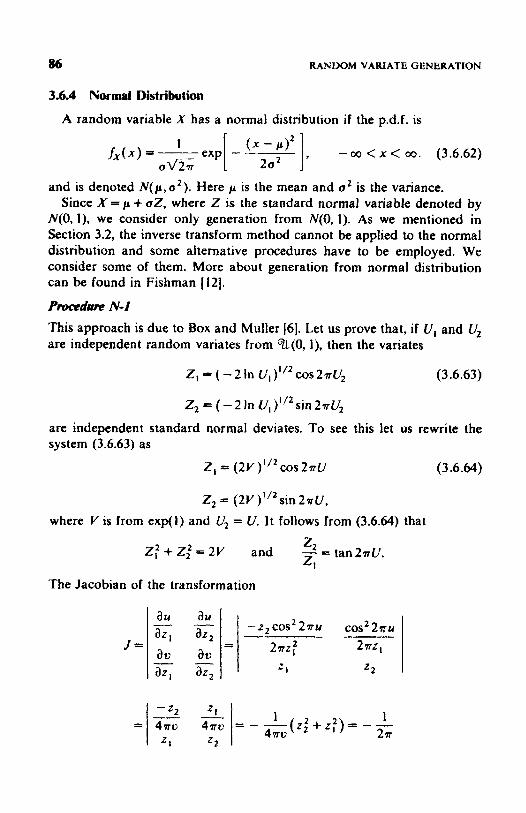
86 RANUOM VARIATE GENERATION
3.6.4 Normal Distribution
A random variable X has a normal distribution if the p.d.f. is
and is denoted N(p.a2). Here p is the mean and u2 is the variance. Since X = p + aZ, where Z is the standard normal variable denoted by
N(0, I), we consider only generation from N ( 0 , I). As we mentioned in Section 3.2, the inverse transform method cannot be applied to the normal distribution and some alternative procedures have to be employed. We consider some of them. More about generation from normal distribution can be found in Fishman [ 121.
Procedure N-l This approach is due to Box and Muller [6]. Let us prove that, if U, and U2 are independent random variates from %(O, I), then the variates
Z , = - 2 In U, cos 2nu2 (3.6.63)
2, = ( - 2 In U, ) 1/2 - sin 2774
are independent standard normal deviates. To see this let us rewrite the system (3.6.63) as
z, = (2V cos 2nU
Z , = ( 2 ~ )"'sin 2 n ~ , where Y is from exp(1) and U, = U. I t follows from (3.6.64)
Z : + Z $ - 2 V and -- ' 2 - tan 2nU. 2,
The Jacobian of the transformation
I - - - ( z ; + z : ) = 1 -- 1 4nv 2n
(3.6.64)
that

GENERATING PROM CONTINUOUS DISTRIBVTIONS 87
and
(3.6.65)
The last formula represents the joint p.d.f. of two independent standard normal deviates.
A/g&thm N- I 1 Generate two independent random variates U, and U, from %(O, I). 2 Compute 2, and Z , simultaneously by substituting U , and U, in the
system of equations (3.6.63).
Procedure 1V- 2
This procedure is based on the acceptance-rejection method. Let the r.v. X be distributed
(3.6.66)
Since the standard normal distribution is symmetrical about zero, we can assign a random sign to the r.v. generated from (3.6.66) and obtain an r.v. from N ( 0 , 1).
To generate an r.v. from (3.6.66) write ,f,( x ) as
,,(.K, = c'h(x)g(-r)
where h( x ) = e --* (3.6.67)
(3.6.68)
(3.6.69)
The efficiency of the method I& equal to Lf.I*/2e ~ 0 . 7 6 . The acceptance condition
u 5 g( Y ) is u 2 exp[ - ( Y - 1),/2], (3.6.70)
which is equivalent to
( Y - 2 ' - I n U 2 (3.6.7 1)
where Y is from exp(1).
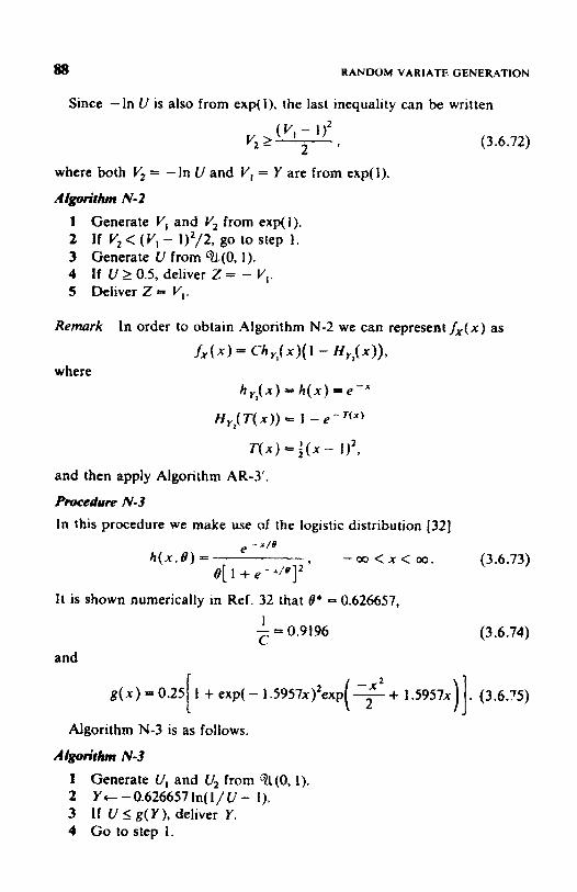
88 RANDOM VARIATE GENERATION
Since -In U is also from exp( 1). the last inequaIity can be written
(3.6.72)
where both Vt = - In U and I/, = Y are from exp( 1).
AIgoritihm N-2 1 Generate V, and V2 from exp(1). 2 If V, < (v , - 1)~/2, go to step I . 3 Generate U from %(O, I). 4 If U 2 0.5, deliver Z = - V,. 5 Deliver Z = Y , .
Remark In order to obtain Algorithm N-2 we can representf,(x) as
f * ( x ) = C b , W ( 1 - N y J x ) ) , where
h y,( x ) = h( x ) = e - x
H , , ( T ( x ) ) = I - e - n x )
T ( x ) = t ( . X - Q2, and then apply Algorithm AR-3‘.
Pmcedurp N-3 In this procedure we make use of the logistic distribution [32]
It is shown numerically in Ref. 32 that 8+ = 0.626657, I - = 0.9196 c
and
(3.6.74)
g(x) = 0.25 I + exp( - i ~ ~ x ) ’ e x p ( $ + 1.5957x)I. (3.6.3) [ Algorithm N-3 is as foliows.
Algorithm N-3 I Generate U, and U, from %(O, 1). 2 Yc-0.626657ln(l/U- I). 3 If U 5 g(Y), deliver Y . 4 Go to step 1.

GENERATING FROM COMINUOUS DISTRIBUTIONS 89
P m d U W N-4
This procedure is based on the relationship between the normal distribu- tion with chi-squared distribution and a vector uniformly distributed on the n-dimensional unit sphere.
Let Z , , . . . , Z , be i.i.d. r.v.3 distributed N(0, I ) and let X = (2:-,Z,?)1/2; then it can be shown by the multivariate transformation method that the vector
Y = = ( Y , ,..., .”)+ = I ,..., ”) X (3.6.76)
is distributed uniformly on the n-dimensional unit sphere.+ Now taking into account that X * = Z;- lZ,’ has the chi-squared distribu-
tion with n degrees of freedom (see Section 3.6.8), the algorithm for generating from N ( O , l ) , where I is a unit matrix of size n, is as follows.
A l g o d h N-4 1 Generate a random vector Y = (Y,, . . . , U,) uniformly distributed on
2 Generate a chi-square distributed random variate xz with n degrees
3 2, - X Y , , k - I , ..., n. 4 Deliver Z = ( Z , , . . . ,Za}.
Since the efficiency of the algorithm for generating Y = (Y,, . . . , Y,) (see example 5, Section 3.4.2) decreases when n increases, it would be interest- ing to find the optimal n in order to minimize the CPU time while sampling from N(0, I).
the n-dimensional unit sphere.
of freedom.
procedrm N-5
This procedure relies on the central limit theorem, which says that if X i , i = l , ..., n,arei.i.d. r.v.’swith E(X,)=pandvar(X,)=a’, then
I - I Z - n”2U
(3.6.77)
converges asymptotically with n to N(0, 1). Consider the particular case
*An alternative algorithm for generating a vector uniformly distributed on the n-dimensional unit sphere is given in example 5, Section 4.3.2.

90 RANDOM VARIATE GENERATION
when all Xi, i = 1 , . . , . n , are from %(O, I). We find that p = f
n
(3.6.78)
A good approximation can already be obtained for n = 12. In this case I2
Z = C V,-6. (3.6;79) I = = 1
Algorithm N-5 is straightforward.
Aigoritlhnt N-S 1 Generate 12 uniformly distnbutcd random variates U,, . . . , U,2 from
%(O, 1). 2 Z+-X!i , l . ! - -6 . 3 Deliver %.
PMdUm N-6
Another approximation technique for generating from N ( 0 , 1) is given in Tocher [33j; it makes use of the following approximation:
(3.6.80) 2e
( I + e
e - v 1 / 2 y
for x > 0 and k = TIT. The c.d.f. for the approximation is
The inverse transformation is 1 1+u X = - I n - k 1 - u - (3.6.8 1 )
Attaching a random sign K to this variate we obtain the desired variate

GENERATING FROM COXTINUOUS DISTRIBVTIONS 91
AlgoritAvn N-6 1 Generate U, and U, from %(O, 1). 2 X + VwT jni(1+ u,)/I - v~>I. 3 If U, 5 0.5, deliver 2 = -X. 4 Deliver Z = X .
3.65 Distribution
with p.d.f. Let X be from N(p, a'). Then Y = e x has the lognormal distribution
0. otherwise. A I ~ i t l C m LN-1
1 Generate 2 from N(0, I). 2 X c p + a Z . 3 Y e e x . 4 Deliver Y.
3.6.6 Cauchy Distribution
equal to An r.v. X has a Cauchy distribution denoted by C(a,p) if the p.d.f. is
, a > o , p > o . - o o < x < O o B =
n[ p + (x - *,'I (3.6.83)
and the c.d.f. is equal to
(3.6.84)
Applying the inverse transform method, we obtain
Algorithm C-1 describes the necessary steps.
Al'dhm C-1
1 Generate U from U(0, 1). 2 X t a - @/tan (vll) . 3 Deliver X.

92 RANDOM VARIATE GENERATION
The next aigorithm is based on the following two properties: (a) If Z , and Z , are independent variates from N(0, I) then Y = Z , / Z ,
is from C(0, 1). (b) If X is from C(0,l) then Y -PX + a is from C(a, / l ) . The last
property can be obtained directIy from the transformation formula (3.5.9)
AIgM'th C-2
1
3 Deliver X . The third algorithm is based on the following property [ 181: (c) If Y, and Y, are independent r.v.'s both from %( - f . +) and
Generate Z, and Z2 from N(0, 1). 2 x+pz,/z, + a.
Y: + Y: 5 f then X = Y, / Yz is from C(0, 1).
Algrn'thm C-3 Generate U, and U2 from DzL(0, 1).
2 Y , t - U , - f and Y 2 t U 2 - , . I
If Y:+ r,2>; go to 1. 4 X t h Y l / Y, + a. 3
5 Deliver A'. The efficiency of the algorithm is
P( r: t. Y; 5;) +, so the algorithm is relatively efficient.
3.6.7 W d W Distribution
An r.v. has a Weibul distribution if the p.d.f. is equal to
0, otherwise and is denoted by W( a, #I). To generate X by the inverse transformation method note that
u = F,( x) 5 1 - e * ( x / f l ) " (3 h.87)
so
x = p ( - t n ( l - u))"". (3.6.88)

GENERATING FROM CONTINUOUS DISTRIBUTIONS 93
Since 1 - U is also from ~%(0, I), we have
or
( $ ) u = -In U. (3.6.90)
Taking into account that -ln(O) is from exp(l), the algorithm for generating an r.v. from a Weibul distribution can be written as follows.
A I m i t k m W-I 1 Generate V from exp( 1).
3 Deliver X. 2 X t p v ” ” .
3.6.8 Chi-square Distribution
Let Z,, . . . ,Z, be from N(0,l). Then k
Y- 2:; (3.6.91)
has the chi-square distribution with k degrees of freedom and is denoted
Formula (3.6.91) says, “the sum of the squares of independent standard normal random variables has a chi-square distribution with degrees of freedom equal to the number of terms in the sum”. One approach for generating a chi-square variate from x 2 ( k ) is to generate k standard normal random variables and then apply (3.6.9 1).
Another approach makes use of the fact that x 2 ( k ) is a particular case of a gamma density with gamma parameters a and equal, respectively, to k / 2 and 2.
i - I
X 2 W
Consider two cases.
CASE 1 If k is even, then Y can be computed as
Y = -2111 11 . (3.6.92)
Formula (3.6.92) requires k/2 uniform variates compared to k in (3.6.91). It also requires one logarithmic transformation, compared to k logarithmic and k cosine or sine transformations .for generating Zi from N(0, l), i = 1,. . . , k (see (3.6.63) and (3.6.64)).
(:I: 1

94 RANDOM VARIATE GENERATION
CASE 2 If k is odd, then k/2 - I / 2
Y=-21n( 1- rI 1 u,)+z2 , (3.6.93)
where Z is from N(0, I ) and ZJ, is from %(O, 1).
For k > 30 the normal approximation for chi-square variates can be used based on the following formula [24):
z = m - V % = - i . Solving for Y. the chi-square variate, we obtain
( Z + m)2 2 Y - (3.6.94)
Remark of freedom 2(a + /3), 2a, and 2p, respectively; then
Let Y , , Y2, and Y, be chi-square random variabies with degrees
has a beta density with parameters a and p. Applying formula (3.6.92), we get
3.6.9 Student’s I Distribution
Let 2 have a standard normat distribution, let Y have a chi-square distribution with k degrees of freedom, and let Z and Y be independent; then
(3.6.95)
has a Student’s t distribution with k degrees of freedom. To generate X we simply generate Z as described in Section 3.6.4 and Y as described in Section 3.6.8 and apply (3.6.95). For k 2 30 the normal approximation can be used.
3.6.10 F Distribution
Let Y, be a chi-square random variable with k, degrees of freedom; let Yz be a chi-square random variable with k, degrees of freedom, and let Y,

GENERATING FROM DISCRETE DISTRIBUTIONS 9s
and Y, be independent. Then the random variable
(3.6.96)
is distributed as an F distribution with k , and k , degrees of freedom. To generate an F variate we first produce two chi-square variates and then use (3.6.96).
Remurk 1. then l / X has an F distribution with k , and k, degrees of freedom.
If X has an F distribution with k and k, degrees of freedom,
Remark 2. degrees of freedom, then
If X is an F-distributed random variable with k , and k ,
(3 6.97)
has a beta density with parameters a = k /2 and /3= k, /2.
3.7 GENERATING FROM DISCRETE DlSTRIBUTIONS
In this section we describe several procedures for generating stochastic variates from must of the well known discrete distributions. We start with the inverse transform method, which Is generafly easily implemented and is widely used.
Let X be a discrete r.v. with probability mass function @.m.f.) Pr ( X = x k ) = P, , k - 0, 1 , . . . (3.7.1)
and with c.d.f. L
8, = Pr(X G x,) - CP, . (3.7.2) 8 I1
Then
where U is from %(O, 1). Thus
X = min { x : g,- , < U s g k } . (3.7.4)
Algorithm IT-2, which is called the inverse transform algorithm, describes generating discrete r.v.'s. This algorithm is based on logical comparison of U with g,'s and is as follows.

96 RANDOM VARIATE GENERATION
Ct Po. B C C . KtO. Generate U from %(O, I). If U I B (U I &), deliver X = x k .
K t K + 1. CCAk + lc Bt B -k c ( Pk + 1 = + 1 'k ).
(8, + 1 = gk + pk+ 1 )' Go to step 5 .
Here Po and A,+ , = PA+ /Pk are distributed dependent. The recurrent formulas
'k i. 1 = A k + I 'k (3.7.5) gk+l =gk + ' k+I (3.7.6)
in steps 7 and 8 are straightforward for calculation.
Most discrete r.v.'s are integers nonnegative valued, that is, xk = k, k = 0, 1,. , . . Later, we consider only these r.v.3. It is easy to see that the mean number of trials
m 00
C = I + x x k P k = Z k P , = l + E ( X ) (3.7 -7) k - I k - l
is equal to the expected value plus one additional trial. Table 3.7.1 represents the values of Po, A,+ I , and C for most well known
discrete distributions. In order to generate an r.v. from a specified discrete distribution, we
take the corresponding values Po and Ak+, from Table 3.7.1 and then run Algorithm IT-2.
In many cases we can improve the efficiency of the inverse transform method IT-2 by starting the search of X at k = m, rn being an interior point (for example, mode, median, etc.), rather than at k = 0. We assume that tables of Pk and gk are available.
The procedure is as follows. If U 2 g,, then gm+t g m + i - 1 + Pm+, (3.7.8)
P,+, = P,+,- IA&+, , i = 1,2,. . . . (3.7.9)
(3.7.10)

4 + L
PI 4 - + c.
4 I 9,
h
4
h
4 Y s
L
4
-. C
2 L N
I C
-.
W
97
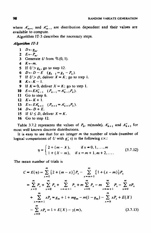
98 RANDOM VARIATE GENfXATION
where A;+, and A:-, are distribution dependent and their values are available to compute.
Algorithm IT-3 describes the necessary steps.
A 1 g ~ i . h IT-3 1 2 3 4 5 6 1 8 9
10 11 12 13 14 15 16
D+gm* E t P , . Generate (I from %(O, 1). K t m . If U > g,, go to step 12.
If U > D, deliver X = K; go to step 1.
If K = 0, deliver X = K; go to step 1. E c E A , " - I Go to step 6. K+K+ 1.
DeD+E. If U 5 D, deliver X = K. Go to step 12.
D + D - E (gk- I =gk - Pk).
K t K - 1.
( Pk- I = A : - I Pk) .
E c E A 4 ; + I ( p k + I = I pk 1-
Table 3.7.2 represents the values of Po, m(mode), A i + l and A i + , for
It is easy to see that for an integer m the number of trials (number of most well known discrete distributions.
logical comparisons of I/ with g: s) is the following r.v.:
(3.7.12) 2 + ( m - X), 1 + ( X - m ) , i f x = m + l , m + 2 ,....
i fxS0, I , ..., m
m ?II W m
= 2 P,+ I;: P,+ P , + M ~ ~ , - m P,- X X P , x - 0 x - 0 n - m + l x = 0 x - m + I x-0
W m
+ 5: x P , = g , + I + m g , - m ( l -gm)- 2 x P x + E ( X ) x - m + I x - 0
m
- xPx" 1 + E ( X ) - y ( m ) , (3.7.13) x-0

Tabl
e 3.7.2
Dis
aete
Uni
mod
ai D
brtri
butio
ss
Dist
ribu
tion
Not
atio
n PO
Mod
al
Val
ue rn
Bino
mia
l
px
= (;
)Px(
l -P
)"-"
x=O
,1, ...
, n,p
>O
Po
isson
e
P, =
-
X!
x=O
,l, .
.., X
>O
N
egat
ive
bino
mia
l
P,-
(x+
;-
I)p'
(l -
p)"
X=
=O
,I, ...
, o<
p<
I
Hyp
erge
ome tr
ic
\ml
max
(O,n
l + m
- n
) s
x 5 m
in(n
,.rn
)
-.P
n-k
k
+l
I-p
h k
+l -
k ,-
n-k
+l
p
k 5; k (
rik
- 1
)(1 -
p)

100 RANDOM VARlATE GENERATION
where m
y ( m ) - 2 2 xPx-g,+m-2mg, . (3.7.14)
It follows from (3.7.7) and (3.7.13) that Algorithm IT-3 is more efficient than Algorithm IT-2 for m such that y( m ) > 0. However, y ( m ) is not necessarily positive for each m.
x - 0
The following example illustrates this point.
Example 1 Assume that the r.v. X has the following p.rn.f.:
p, x = o
0, otherwise.
Let m = 1; then y ( l ) = 2 2 ~ , 0 x P x - g , + 1 -2g,,,- 1 - f + 1 - f - -0.25 < 0, and therefore Algorithm IT-2 is more efficient than Algorithm IT-3.
Neverthetess, in many cases it is possible to choose the starting point m in such a way that y ( m ) > 0, and therefore it is possible for IT-3 to be more efficient than IT-2.
Lemma 3.7.1 I f there exist m > 0 such that rn
.x- I P,I Z: ( 2 % - ij& forg,<;, (3.7.15)
then y ( m ) > 0.
Proof Condition Po 5 Z'$ ,(2x - 1)P' is equivalent to m
2 I= x p x - g , > o , x-0
and, correspondingly, condition g, 5 f , m > 0, is equivalent to
(3.7.16)
m - 2mg, > 0. (3.7.17)
Q.E.D. Both (3.7+16) and (3.7.17) yield y ( m ) > 0.
Note I We can see that Lemma 3.7.1 is valid if Po 5 2:- ,Px.

GENERATING FROM DISCRETE DIS'TRIBU'I'IONS 101
This condition is not restrictable and holds for practically all discrete distributions.
Lemma 3.7.2 y ( m ) achieves its maximum at points mo or m,+ 1 where mo = max ( m : g , 5 i), depending, correspondingly, on whether gm0+ gm,+ i 5 I O r ~ m , + g m , + t > 1.
Prooj It is straightforward to obtain from (3.7.14) that
AY( m ) = ~ ( m + 1) - Y( m ) = 1 - g m - gm+ I - (3.7.18)
For m < mo we have g, + g,+ 5 1, and therefore Ay(m) 2 0; for m > mo we have, correspondingly, g, + g,+ I > I and Ay(m) < 0. Therefore y(m) is a unimodal function with the maximum at points m, or mo+ I , depending on whether gm0 + gm0 + I I 1 or gma + gm0 + I > 1. Q.E.D.
Nore 2 mum at the median or at a point neighboring the median on the left.
In other words, Lemma 3.7.2 says that y ( m ) achieves its maxi-
As a corollary from these two lemmas we obtain the following theorem.
Tbeorem 3.7.1 The optimal starting point in Algorithm IT-3 is either the median mo= max { m : g , S i } , if Po 5 Z::;'(2x - IjP, and gm0+ gme+l s 1, or mo + 1, if Po I Z,ol m + I (2x - 1)P. and ~ Q ~ ~ + R ~ ~ + ~ > 1.
Nofe 3 Theorem 3.7.1 is valid not only for integer nonnegative valued r.v.'s, but for any discrete r.v. with values xO,x,, . . . , since Algorithm IT-3 is determined not by the sequence x,, x I . . . . , but by its indices 0, 1, . . . .
In the rest of this chapter we consider some alternative procedures for generating discrete r.v.'s. Generally, procedures for generating discrete variates are simpler than procedures for generating continuous variates, and we describe them only briefly.
3.7.1 Binomial Dtstrfbution
An r.v. X has a binomial distribution if the p.m.f. is equal to
P, = (;)p"(l - p ) " - - I , x 5 0, ... , n (3.7.19)
and is denoted by B(n ,p ) . Here 0 < p < 1 is the probability of success in a single trial, and n is the number of trials.
To apply the inverse transform method IT-2 we must check the follow- ing condition after step 5: if K- n - 1, terminate the procedure with X = K - n .

I02 RANDOM VARIATE GENERATION
It is also worthwhile to note that. if Y is from B(n ,p ) , then n - Y is from B(n, 1 - p ) . Hence for purposes of efficiency we generate X from B ( n , p ) according to
~ - ~ ( n ! p ) i f p ~ ; $
y--B(n, 1 - p ) ifp >f. (3.7.20)
For larger n the inverse-transform procedure becomes time consuming, and we can consider the normal distribution as an approximation to the binomial.
As n increases the distribution of
(3.7.2 1)
approaches N ( 0 , 1).
with respect to X, and round to nonnegative integer, that is,
X = max (0, [ -0.5 + np + Z(np( 1 - p ) ) ” 2 ] ) ,
To obtain a binomial variate we generate Z from N(0, I), solve (3.7.21)
(3.7.22)
We should consider replacing the binomial with the approximate normal
It is shown [22] that, if m is the mode, then for large n the mean number
where [a] denotes the integer part of a.
when np > 10 forp >-f and n(1 - p ) > 10 forp <:.
of trials in Algorithm IT-3 is equal to
(3.7.23)
Comparing both Algorithms IT-2 and IT-3 (compare (3.7.7) with (3.7.23)). we can see that for large n the mean number of trials is proportional to np and im, respectively.
So for large n Algorithm IT-3 is essentially more efficient than Algo- rithm IT-2.
The acceptance-rejection method can also successfully be implemented for generating from B ( n , p ) (see Ahrens and Dieter [4] and Marsaglia 1201). Description of algorithms for this and their efficiency can be found in Fishman’s monograph [ 121.
3.7.2 Poisson Distribution
An r.v. X has a Poisson distribution if the p.m.f. is equal to
x = 0,1,. . . ; h > 0 (3.7.24) Axe -’ P, = -
x ! ’ and is denoted by P(A) .

GENERATINO FROM DISCREl'E D1SlRIBU'l'tONS 1 03
I t is well known (Feller (111) that, if the time intervals between events are from exp(l/X), the number of events occurring in an unit interval of time is from P ( h ) .
Mathematically, it can be written X x * I
X q 5 1 5 2 I r ; , i = O i -0
(3.7.25)
where T,, i = O , 1 , ..., X + 1, are from exp(I/X). Since = -(l/X)ln V,, the last formula can be written as
X x + I
i -0 i = O - InY < A < - lnV,, X = O , l , ... (3.7.26)
or
(3.7.27)
The following algorithm is written with respect to (3.7.25):
1 A + l ( # k = 1). 2 KcO. 3 Generate Uk from %{O, 1).
5 If A < e-', deliver X = K. 6 K t K + 1. 7 G o to step 3.
For large h(h> 10) we can approximate the Paisson distribution by
A c - U k A ( g i , + I m g k U k ) '
normal distribution. As X increases, the distribution of
(3.7.28)
approaches N(0, 1).
with (3.7.22) we obtain To obtain a Poisson variate we generate Z from N(0, I ) , then by analogy
(3.7.29)
It is shown in Ref. 22 that, if m is the mode, then for large n the mean
x = max (0, [ x + z''~ - OS]),
where [a] is the integer part of a.
execution time in Algorithm IT-3 is similar to (3.7.23) and is equal to
(3.7.30)

104 RANDOM VARlATE GENERATION
The mean number of trials in both Algorithms IT-2 and IT-3 are proportional, respectively, to X and A'", and therefore Algorithm IT-3 is again essentially more efficient than Algorithm IT-2.
3.73 Geomebrc . Distribution
An r.v. has the geometric distribution if the p.m.f. is equal to
P x = p ( l - p ) " , x=O,l , ..., o < p < I (3.7.3 1) and is denoted by Ge(p) . Geometric distribution describes the number of trials to the first success in a serial of Bernoulli trials,
The following procedure describes generating from Ge(p) and is based on the relationship between exponential and geometric distribution. Let Y be from exp(/?); then
(3.7.32) which is G e ( p = 1 - e - ' ' f l ) .
For /3 = - 1 /In ( 1 - p ) (3.7.32) is identical to (3.7.3 I). Therefore
(3.7.33)
where V = -In(U) is a standard exponential variate, that is, X is from Ge( p). Hence to generate an r.v. from G e ( p ) we generate an r.v. from the exponential distribution with /3 = - I /ln ( I - p ) and round the value to an integer.
CPU time for this procedure is constant, whereas the CPU time for the inverse transform method is proportional to l / p . However, because this procedure requires generation from the exponential distribution and rounding, it is more efficient than Algorithm IT-2 only for p < 0.25.
3.7.4 Negative Binomid Distribution
The p.m.f. for the negative binomial distribution is
P x = ( x + r - X I ) f ( l --p)", X'O,l,. . . ; p > o (3.7.34)
and is denoted by N B ( r , p ) . When r is an integer the distribution is called Pascal distribution, which describes the number of successes occurring before the rth failure in a series of Bernoulli trials. This implies that geometric distribution is a special case of Pascal distribution with r = 1.

GENERATING FROM DISCRETE DISTRIBUTIONS 1oJ
The following algorithm describes generating from Pascal distribution with parameters r and p denoted PS(r,p) .
1 X t O . 2 YCO. 3 Generate Ox+ from %(O, I). 4 If U,, > p , go to step 8. 5 Y C Y + I . 6 If Y = r, deliver X. 7 Go to step 3. 8 X t X + l . 9 Go to step 3.
An alternative procedure is based on the reproducfiw property of the negative binomial distribution analogous to that for the gamma distribu- tion. Let X, , i = 1,. . . , n , denote a sequence of i.i.d. t.v.’s from NB(r,,p). Then X = 2:- I X, is from PS( r , p ) , where r = 2:- !r,.
Suppose that r, = 1, i = 1,. . . , r, which means that X,, i = 1,. . . , r , are from C e ( p ) ; then X = Z : , , X , is from NB(r ,p ) .
The algorithm is straightforward and contains the following steps:
1
3 Deliver X.
Generate X,, . . . , X, from Ge( p ) . 2 x+-z;olx,.
This procedure is more efficient than the inverse transform method IT-2 for p > 0.75.
Another possible method for generating an r.v. from NB( r , p ) makes use of the following relationship (see Johnson and Kotz [ 18, p. 1271):
Pr ( X I k ) = Pr ( Y 2 r ) , (3.7.35)
where X is from N B ( r , p ) and Y is from B( p , r + k ) . The reader is asked to describe an algorithm based on (3.7.35), assuming that r.v. Y from B ( p , r + k ) is given.
The next procedure is based on the relationship between negative
Suppose we have a mixture of Poisson distributions, such that the binomial distribution with gamma and Poisson distributions.
parameter X of the Poisson distributions
x = o , I , ... e -’V P ( X = x l X ) =-
x! ’

106 RANDOM VARIATE GENERATION
varies according to G( a, p), that is,
X 2 0,a > 0, #3 > o . (3.7.36)
Then
P( X = x) = i w P ( X = xlh)f , (A)dA (3.7.37)
= P V 4 3 -
So Xis from N B ( a , 1/(P+ 1)).
(3.7.34). The algorithm is as foIlows: It is obvious that, when A is from G ( r , (1 - p ) / p ) , (3.7.37) is identical to
1 Generate an r.v. X from G ( r , p / ( I - p ) ) 2 Generate X from P(A). 3 Deliver X.
I t is not difficult to see that an alternative algorithm for generating an r.v. from N B ( r , p ) is the following:
1 Generate A from G(r , 1). 2 Generate X from P ( X p / ( l - p ) ) 3 Deliver X.
3.7.5 Hypergeometric Distribution
An r.v. X has a hypergeometric distribution if the p.m.f. is equal to
, max(O,n, + m- n) I x 15 min(n, ,m) P, = ( ",--": ) (9
(3.7.38)
and is denoted H( n. m, nt). Hypergeometric distribution describes sam- pling without replacement from finite population. i t has three parameters, n, m, and n, , which have the following meanings: n, the size of the total population in two classes, rn, the size of the sample (m < n ) that is taken from the total population n without replacement, and n,, the size of the

EXERCISES 107
population in the first class ( n - tz, is the size of population in the second class).
Generation from H(n, m, n , ) involves simulating a sampling experiment without replacement, which is merely a Bernoulli trials method of generat- ing from B(n,p) with n andp altering (varying) depending, respectively, on the total number of elements that have been previously drawn from the total population and the number of the first class elements that have been drawn.
The original value n = no is reduced according to the formula n , = = n i w I - I , i = I ,..., m (3.7.39)
when an element in a sample of m is drawn.
elements is drawn, becomes Similarly, the valuep =po = n , / n , when the ith element in a sample of n
n i - Ipi - l - 6 n , - l - 1
, i = 1 ,..., M , Pi = (3.7 .#)
where S = I when the sample elements ( i = I ) belong to the first class, and 6 = 0 when the sample elements ( i - I ) belong to the second class.
1 Describe an algorithm lor generating from Laplace (double exponential distri- bution)
, B > O , - 0 0 4 x < < .
using the inverse transform method
tion 2 Apply the inverse transform method for generating from extreme value distribu-
3 Describe an algorithm for generating from logistic distribution
4 Consider the triangular random variable with the density function
if x < 2a or x 2 2b if 20 I x < a + b x - 2 a
(26 - X) if a + b s x < 26,

108 RANDOM VAR3ATE GENERATION
F d x ) = +
and the distribution function
if 2a I x < a + b ( x - 2 ~ ) ~ 2( b - a)2 ’
I - (26 - x ) ~
2 ( b - a J 2 if a + b 2 x < 26
Ill i f x 2 2 b
This random variable can be considered as a sum of two independent random variables uniformly distributed between a and b. Show that, applying the inverse method, we obtain
2a + ( b - a ) 6 U if05 W ~ 0 . 5
2 b + ( a - b ) < 2 ( 1 - U ) , i f O . S c U < I . 5 Let
C,X, X , - , I X S X ~ , i 5 1 , ...* n
’xix).p { 0, Otherwise x o = a , x , = b , c , k O , a 2 0 .
Using the inverse transform method, prove that
where F, = Z:, I $2- ,c,x dx. Describe an algorithm for generating from jx( x),
6 k t X ,,..., X, be i.i.d. r.v.’s from exp(A).
(a) Show that Y , = min ( XI,. . . , X,) is distributed exp ( n X ) . (b) Describe an algorithm for generating from Y,.
from Be( a,@).
Show that their ratio X/W has a Cauchy density.
Section 3.4 by making use of Theorem 3.4.2.
10 Describe algorithms for generating from the following p.d.f.’s:
(a) j x . y ( x , y ) = c e - ( x + Y ) , x r O , y 20. @) / x u ( x y ) = c x e c x y , 0 5 x 5 2 , y 2 0. (c) For generating from N ( p , X ) where 1 r = ( ~ , , l ~ ~ , p , ) = ( l , 2 , 3 ) , and
7 Lct U , , . .., U,+,-, be from %.(a. 1). Prove that the ath order statistic C&, is
8 The joint density of the r.v.’s X and Y is of the fonnf(uz + d) for all u and u.
9 Describe two alternative algorithms, correspondingly, for examples 4 and 5 of
1 1 0 x - I 2 0 .
i o 0 31
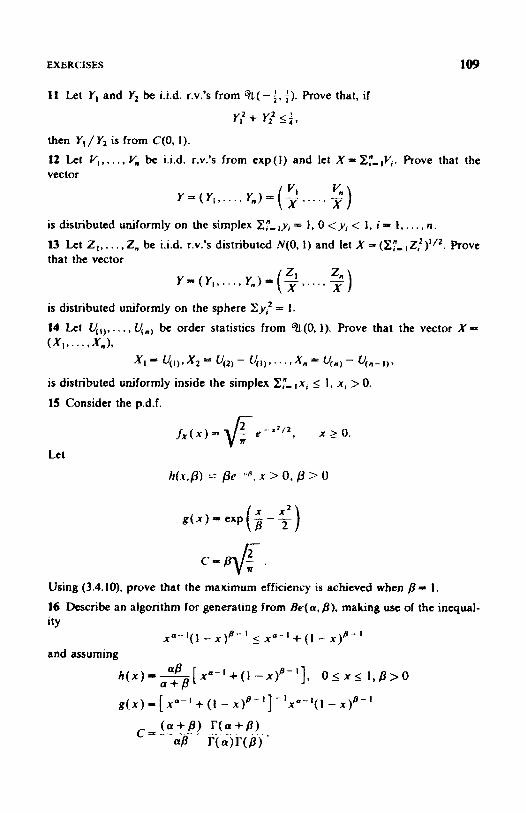
EXERCISES 109
11 Let Yl and Y2 be i.i.d. r.v,'s from %( - 4, i). Prove that, if
Y:+ Y 2 ' 5 i ,
then Yl / Y2 is from C(0, 1).
12 Let V, ,..., V, be i.i.d. r.v.'s from exp(l) and let X=z: - ,V i . Prove that the vector
Y = ( Y [ , ..., Y " ) = ( s x ' . * " 5) X
is distributed uniformly on the simplex 2;- ,y , = I , 0 <yi < 1, i - I , . . . , n. 13 Let Z,, . . . ,Z, be i.i.d. r.v.3 distributed NfO, 1) and let X = (2;- ,Z:)'/*. Prove that the vector
Y = ( Y I , . . . , Y n ) - ( 2 ,..., 3) X
is distributed uniformly on the sphere Zy: = 1 .
14 Let Yt,, . . . , y , , be order statistics from %(O, I) . Prove that the vector X = ( X , t . . . 1 X").
X I 5 q,),x* = y 2 , - y l ) , . . . ,X" = q", - qn-,t, is distributed uniformly inside the simplex 2:, ,x, I I , x , > 0. 15 Consider the p.d.f.
Let
Using (3.4. lo), prove that the maximum efficiency i s achieved when /3 = I . 16 Describe an algorithm for generating from &(a,@}, making use of the inequal- ity
and assuming x"-'(l - - x f - ' 2 x * - I + ( I - X)+'
h ( x ) = - [ x " - ' + ( l aB - x y - q , o l x l l , p > o
g ( x ) = [ x" - I+ ( I - x y - '1 - k'( 1 - x y - 1
a + p

110 RANDOM VARXATE GENERATION
Compare the efficiency of this procedure with the efficiency of Johnk's procedure, B e 4 17 Describe an algorithm for generating from G(a, 1) by the acceptance-rejection method AR-I, assuming
h ( x ) - p E 4 B , m ) + (1 - P ) W P , m + 11%
that is, h ( x ) is a mixture of two Erlang distributions, where m = [a] and P = a / m .
18 Prove that Procedure Be-6 i s more efficient than Procedure Be-5 for a 2 2, B z 2 . 19 Rescribe an acceptance-rejection algorithm for generating an r.v. from N(0, l), representingf,(x) = Cg(w)h(x,P) and assuming that
m < x < m .
Verify that the optimal @ = I , the efficiency I/C = e'/'/
g(x)==0.8243(1 +xZ)e-X2/2.
= 0.6578, and
From Tadikamalla and Johnson [32]. 20 Describe an algorithm for generating from truncated Erlang distribution
m -- te - x / B x > l , B > O , m = 1 , 2 ,...,
@"(m - I ) ! ' fx(x) c
and find c.
21 Prove that, ifj'(x) can be represented asfx(x)== Ch,,(xWl - ff,J'f(x))], then Algorithm AR-3 can be rewritten as AR-3'. 22 The p.rn.f. for the uniform discrete distribution is
x = u , a + 1 ,..., 6 , t P x p b - u + 1
where b and u are integers and b > u. Prove that X =[a + ( b - u + 1)UJ has the desired distribution, and describe an algorithm for generating an r.v. from P,. Here [a] is the integer part of a.
23 Let Y be from Bernoulli distribution, that is,
P,=pY(I -p)? y = O , l , O < p < 1.
Prove that, if Y , , . . . , Y, are i.i.d. r.v.'s from Bernoulli distribution, then X - C;, ,x is from B(n,p) . Describe an algorithm for generating an r.v. from B ( n , p ) , using the above result. For purposes of efficiency use the fact that if X is from B(n,p) , then n - X is from B ( n , I - p ) .
24 Prove (3.7.25), that is, if the time intervals between events are from exp(l/h), then the number of events occurring in a unit interval of time is from P(h) .

REFERENCES 111
ZJ Prove that y = x81(l - X ) ~ > is a concave function on (0,1] and has a maximum equal to
26 t e t X and XI be i.i.d. r.v.'s and let Y = aX + ( I - a ) X , , where 0 5 1.1 Prove that the correlation coefficient
I .
a P X , Y = $W.
Describe an algorithm for generating a pair of r.v.'s (A'. Y) for which p x v = p. 27 Prove Theorems 3.4.2 and 3.4.3.
28 By analogy with Theorem 3.4.2 formulate a theorem that is a multidimensional version of Algorithm AR-I, and prove it. 29 Let X = (X,, . , . , A',,) be i.i.d. r.v."s uniformly distributed inside a n n-dimensional unit sphere. Prove that the vector Y = C S i s uniformly distributed inside the ellipsoid
where Z is a symmetric and positively defined ( n X n) matrix and C is the lower triangular matrix (3.5.13). such that B - C'C. Hint: Use the fact that the vector W = ( WI.. . . , W,) - KX is uniformly distributed inside the n-dimensional sphere
Y T Z Y 5 K2,
WrW p W: +. W: +. . . + W: 5 K 2 with radius K.
REFERENCES
Ahrens, 3. H. and U. Dieter, Computer methods for sampliq from the exponential and normal distributions, Comm. A s ~ o c . Comp. Mach., 15, 1972. 873-882. Ahrens, J. H. and U. Dieter, Extensions of Fonytbe's method for random sampling from the normalldistribution, Math. Cow., 27, 1973, 927-937. Ahrene, J. H. and U. Dieter, Computer methods for sampling from gamma, beta, poisson and binomial distributions, C-ring, 12. 1974, 223-246. Ahrcns. J. H. and U. Dieter, Non-Unifonn RMdono Numbers, Institut fk Mathematiache Statist&. Technixhe Hochschulc in Graz, Austria, 1974. A n d e m , T. W., An Intr&rion to Mdtiwriote Storisticol AnolyJir, Wiley, New York, 1958. Box, G. E. P. and M. E. Muller, A note on the generation of random normal deviates,
Butler, J. W., Machine sampling from given probability distributions, in Synposim on Monte Corlo Mef&, edited by M. A. Meyer, Wiley, New York. 1956. Chcng, R. C. H., Generating Beta variates with non-iotegral shape parameters, Comm. Assoc. Comp. Mach,, 21, 1978. 317-322.
A M . Math. S I ~ . , 29, 1958, 610-611.

112 R A N W M VARIATE GENERATION
9 10
11
12 13
14
15
I6
17 18
19
20
21
22
23
24 25 26
27
28
29 30
31
32
33
Cheng, R. C. H., The generation of gamma variables, AppL Stut., 26, 1977,71-75. Ermakw, J. M., Mottle Carlo Method and Related Questions, Nauka, Moscow, 1976 (in Russian). Feller, W.. An Intmdwtion ro Probobilify 2 k o y and 10 &lications, Wiley, New Yak, 1950. Fishman, G. S., Principles of Discrete Ewnr Simuhtwn, Wiky, New Yo&, 1978. Fishman, 0. S., Sampling from the gamma distribution on a computer, C o r n . ICWUK..
Fishman, G. S., Sampling from the Poisson distribution on a computer, Conlputing, 17,
ForsytbG G. E.. Yon NCUXIUM’S comparison method for random samphg and from the normal and other distributions,” Math. Cq., 26, 1972, 817-826. JGhnk, M. D., Erzeugung von Betraver(eiIten and Gammamtcilten Zuffa ldcn, Metrika, 8, 1964, 5- IS. Johnson. N. L. and S . KO@, Discrete Disrributiau, Houghton-Mifflin, 1969. Johnson, N. L. and S. Kotz, Continuour Unicariate Distriktim,Vols. 1 and 2, Houghton- Mifflin, 1970. Marsagha, G., Generating exponential random variables, Ann. Math. Staf., 32, 1961,
Marsagha, G.. Generating discrete random variables in a computer, Comm. Assm. C m p .
Mamaglta, G., M. D. MacLaren, and T. A. Bray, A fast p r d u r e for generaling normal random variables, Comm. Asw. Contp. Mach., 7, 1964. Michailov, S. A., Some Prvbtenu in the l”hew o/ the M w e Carlo Metho&, Nauka, Novosibirsk, U.S.S.R., 1974 (in Russian). Mood. A. M., F. A. Graybill, and D. C. Boes, Inrr&ticm to rhe l”heqv oj Statistim, 3rd td., McGraw-Hill, New York. 1974, 4- 10. Naylor, T. H . et al.. Conylurer Simulation Tkchniques, Wiley, New York, 1966. Ncuts, M., Probabiliry. AUyn and Bacon, 1972. philips, D. T. and C. Beightlcr, Procedures far generating gamma variates with non-integer parameter sets, J. Stat. C q . Sirnulorion. 1912, 197-208. Reks, D., A simple algorithm for generating binomial random variables, J. A m r . Stat.
Robinson. D. W. and P. A. W. h i s , Generating $amma and Cauchy random variables: An extension to the Naval Postgraduate School random number package, 1975. Sobol, J. M., Cmputationa! Methook of Monre Carlo, Nauka, Moocow, 1973 (in Russian). Tadikamalla, P. R., Computer generation of gamma random variables, Comm. Assoc. COT. Mach., 21, 1978, 419-422. Tadikamatia, P. R., Computer generation of gamma random variabkq 11, Comm. Assoc. Conip. Mach., 21, 1978,925-928. Tadikamalla, P. R., and M. E. Johnson, Simple rejection methods for sampling from the normal distribution, in Prmeedngs of the Firsr Inietnatiowl Conference of Mathematical Modeling, X. J. A d a , Ed., St. Louis, Missouri, 1977, 573-577. Tocher, K. D., The Art of Simulation, Van Nostrand, Princeton, New Jersey, 1963.
Conip. Mwh., 19, 1976,407-409.
1976, 147- 156.
899-900.
Mmh., a, 1963,37-38.
ASSM., 67, 1972,612-613.

REFERENCES 113
34 VOD Neumana, J.. Various techniques used in connection with random digits, U.S. Not. Bur. Stand. Appl. Math. Ser., No. 12, pp. 36-38, 1951.
35 Wallace, N. D., Computer generation of gnmma random variates wih non-integral shape jmrameters, Comm. Assoc. Cmp. Mock. 17, 1974,691495.
36 Walker. A. J., An efficient method for generating discrete random variables with general distributions, T m . Moth. Sofrware, 3, No. 3, Stptcrnbcr 1977.253-257.
37 Whittaker, I., Generating gamma and beta raudom variables with non-integrable shape parameters, Appl. Stat., 23, 1974. 210-214.
38 Wilde, D. J., Optimum Seeking Methodr, Rcntice-Hall. Englcwood Cliffs, New Jersey, 1964.
39 Yakowitz, S. J., Cowputotion Pmbabiiiity and Simuklrion, Addison-Wdy, Reading, Massachusetts, 1977.

C H A P T E R 4
Monte Carlo Integration and Variance Reduction Techniques
4.1 INTRODUCI‘ION
The importance of good numerical integration schemes is evident. There are many deterministic quadrature formulas for computation of ordinary integrals with well behaved integrands. The Monte Carlo method is not competitive in this case.
But if the function fails to be regular (i.e., to have continuous derivatives of moderate order), numerical analytic techniques, such as the trapezoidal and Simpson’s rules become less attractive. Especially in the case of multidimensional integrals, application of such rules (formulas) runs into severe difficulties. I t is often more convenient to compute such integrals by a Monte Carlo method, which, although less accurate than conventional quadrature formulas, is much simpler to use.
It is shown that each integral can be represented as an expected wlue (parameter) and the problem of estimating an integral by the Monte Carlo Method is equivalent to the problem of estimating an unknown parameter. For convenience we use the expression “estimating the integral” rather than “estimating the unknown parameter.” In Section 4.3.12 we consider several practical examples of estimating such parameters (integrals).
114
Simulation and the Monte Carlo Method R E W E N Y. RUBINSTEIN
Copyright 0 1981 by John Wiley & Sons, Inc.
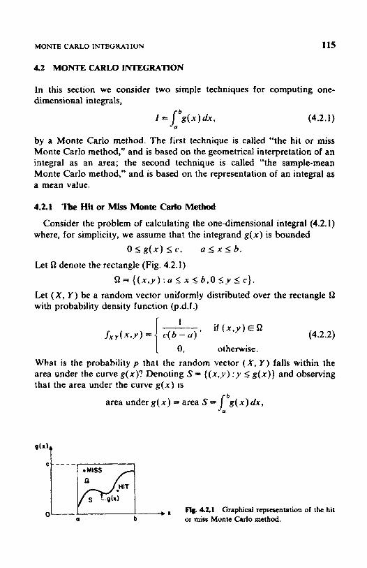
MONTE CARLO INTEGRATION 115
4.2 MONTE CARLO INTEGRATlON
In this section we consider two simple techniques for computing one- dimensional integrals,
I = f 6 g ( x ) d x , (4.2.1)
by a Monte Carlo method. The first technique is called “the hit or miss Monte Carlo method,” and is based on the geometrical interpretation of an integral as an area; the second technique is called “the sample-mean Monte Carlo method,” and is based on the representation of an integral as a mean value.
a
4.2.1 Tbe Hit or IMiss Monte Carlo Method
Consider the problem of calculating the one-dimensionat integral (4.2.1) where, for simplicity, we assume that the integrand g ( x ) is bounded
O I g ( x ) _ < c . a I x I 6 .
Q = { ( x , y ) : u < x I b , o 5 : ~ Y r e ) . Let fi? denote the rectangle (Fig. 4.2.1)
Let (X, Y) be a random vector uniformly distributed over the rectangle S2 with probability density function (p.d.f.)
(4.2.2)
otherwise. What is the probability p that the random vector ( X , Y) falls within the area under the curve g(x)? Denoting S = { ( x , y ) : y I g ( x ) ) and observing that the area under the curve g(x) is
a r e a u n d e r g ( x ) = a r e a S = i b g(x)d.x,
c - - _ _
- g M
Fig. 42.1 Graphical representation of the hit
i ~ . ‘ a b or miss Monte Carlo method.

116 MONTE CARL0 INTEGRATION AND VARIANCE REDUCTION TECHNIQUES
we obtain
(4.2.3)
Let us assume that N independent random vectors ( X , , Y,), ( X , , Y2),. . . , ( X N , YN) are generated. The parameter p can be estimated by
(4.2.4)
where NH is the number of occasions on which g ( X , ) 2 6 , i = 1,2,. . . , N, that is, the number of “hits,” and N - NH is the number of “misses”; we score a miss if g( X i ) < y i , i = 1,. . . , N, as depicted in Fig. 4.2.1.
It follows from (4.2.3), and (4.2.4) that the integral Z can be estimated by
(4.2.5) 1-49, = c( b - a)-.
In other words, to estimate the integral I we take a sample N from the distribution (4.2.2), count the number N,, of hits (below the curve g(x)) , and apply (4.2.5).
Since each of the N trials constitutes a Bernoulli trial with probability p of a hit, then
$I- NH N ’
NH N
(4.2.6)
that is, 8, is an unbiased estimator of 1. The variance of p is
which, together with (4.2.3). gives
[ c ( b - a ) - I ] . 1 Z varb = -
[ c ( b - a ) ] * (4.2.8)
Thus
var8, = [ c ( b - a)I2 var$ = [ c(b - a)I2-!-p( 1 -p) (4.2.9) N I N = - [ c(b - a ) - 11
and the standard deviation
% = [var 8, 1 ’’, = N - ‘ / 2 { Z( c(b - a ) - I ] 1 ”,.
MONTE CARL0 INTEGRATION 117
Note that the precision of the estimator 8,, which is measured by the
How many trials do we have to perform, according to the hit or miss
P [ l e , - q < & ] (4.2.10)
inverse of standard deviation, is of order N -'I2.
Monte Carlo method, if we require
Chebyshev's inequality,
together with (4.2.10), gives var ff,
E2
Substituting (4.2.9) in (4.2.12), we obtain
a S l - - - ,
P ( 1 - P ) [ C @ - 4 1 2 a l l - N E ~
Solving (4.2.13) with respect to N, we have
(4.2.1 I )
(4.2.12)
(4.2.13)
(4.2.14)
which is the required number of trials for (4.2.10) to hold.
which says that for N sufficiently large the random variable (r.v.) When N is sufficiently large we can apply the central limit theorem,
(4.2.15)
is distributed approximately according to the standard normal distribution, that is,
P ( 0 , I x ) ==+(x). (4.2.16)
where 1 s
+(x)=-/ e - r f /2dr . (4.2.17)
We can easily verify that the confidence interval with level 1 -2a for I is f i n --c9
(4.2.18)
where
z a = + - ' ( a ) * (4.2.19)

118 MONTE CARL0 INTEGRATION A N D VARIANCE REDUCTION TECHNIQUES
Hammersley and Handscomb [ 101 write:
Historically, hit or miss methods were once the ones most usually pro- pounded in explanation of Monte Carlo techniques; they were of course, the easiest methods to understand (particularly if explained in the kind of graphical language involving a curve in a rectangle).
Nit or Miss Monte Cado Method A I g d h m 1 2 Arrange the random numbers into N pairs (U,, U;),
(U2, U;), . . . ,(U,, U;) in any fashion such that each random number U, is used exactly once.
3 Compute
Generate a sequence { r/i}:,”, of 2 N random numbers.
X , = a + V , ( b - a ) and g ( X i ) , i = 1 , 2 ,..., N. 4 Count the number of cases NH for which g ( X , ) > cq.‘. 5 Estimate the integral I by
NH 8, = c (6 - a ) - N
4.2.2 The Sample-Man Monte Carlo Method
Another way of computing the integral
I = J b g ( . r ) d x a
is to represent it as an expected vaiue of some random variable. Indeed, let us rewrite the integral as
(4.2.20)
assuming thatjx(x) is any p.d.f. such thatf,(x) > 0 when g(x) ZO. Then
where the random variable X is distributed according to f x ( x ) . Let us assume for simplicity
if D < x < 6,
otherwise;
I
(4.2.21)
(4.2.22)
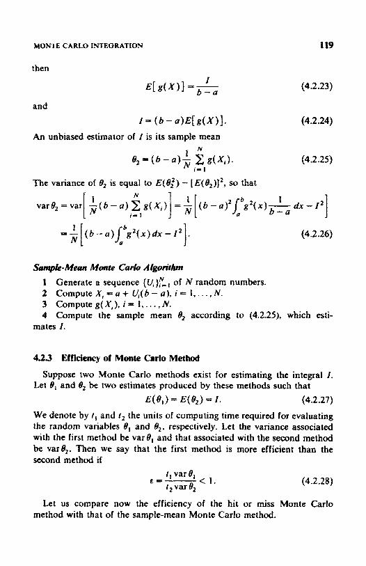
MONTE CARLO INTEGRATION 119
then
(4.2.23)
and
An unbiased estimator of I is its sample mean s N
(4.2.25)
The variance of 8, is equal to E(6:) - [E(f?,)]’, so that N 1 var 8, = var [ ( b - u ) g ( X i ) ] = A [ ( 6 - u) ’ l”p ,( x ) b-a
is= I
Sanr;ple-Mean Monte Carl0 Algunthm
1 Generate a sequence {V,>,”-, of N random numbers. 2 Compute X , = a + Q ( b - a), i== I ,..., N. 3 Compute g( X,), i = I , . . . , N. 4 Compute the sample mean 0, according to (4.2.25), which esti-
mates I.
4.23 Efficiency of Monte Carlo Method
Let B , and 8, be two estimates produced by these methods such that Suppose two Monte Carlo methods exist for estimating the integral 1.
q e , ) = qe , ) = I . (4.2.27)
We denote by I , and f , the units of computing time required for evaluating the random variables 8, and 6,. respectively. Let the variance associated with the first method be var 8, and that associated with the second method be var8,. Then we say that the first method is more efficient than the second method if
I , varb, €5- < I .
t t var 8, (4.2.28)
Let us compare now the efficiency of the hit or miss Monte Carlo method with that of the sample-mean Monte Carlo method.

120 MONTE CARLO INTEGRATION AND VARWNCE REDUCTION TECHNIQUES
Propodtho 4.2.1 var 8, I var B,.
Proof Subtracting (4.2.26) from (4.2.9), we obtain
(4.2.29)
Note that
therefore
and further var 8, - var 8, 2 0. Q. E. D.
Assuming that the computing times 1 , and t , for 8, and 0, are approxi- mately equal, we conclude that the samplemean method is more efficient than the hit or miss method.
If var 8, and var 8, are unknown, we can replace them by their estima- tors
(4.2.3 1) I’ N 2 g( Xi)( b -- a ) - 6
and then estimale by
11 s: E J - (4.2.32)
It is interesting to note that, estimating the integral by 8, and S,, we do not need to know the function g(x) explicitly. We need only evaluate g(x) at any point x.
4.2.4 Integration in the Presence of Noise
Suppose now that g(x) is measured with some error, that is, we observe g(x,) = g ( x i ) + ei, i = 1,2,. . . , N, instead of g, where ei are independent identically distributed (i.i.d.) random variables with
E ( E ) = 0, var ( E ) = u 2 (4.2.33)
and IEf < k < 00. (4.2.34)

VARIANCE REDUCTION TECHNIQUES 121
Let ( X , Y ) be a random vector distributed
otherwise, where
c, 2 g(x) + k. Then, by analogy with 8, for the hit or miss method, we obtain
NH ” 8, ~ , ( 6 - a ) - (4.2.35)
where N,, is the number of hits, that is & X i ) 2 K., i = I , . . . , N. By analogy with f12 for the sample-mean Monte Carlo method with
a l x S 6
otherwise, we obtain
N 1 N 8, =---(!I - a ) i ( X i ) .
I - 1 (4.2.36)
We can show that both r.v.’s 4, and 8, are unbiased and converge almost surely (as.) and in mean square to I and that the sample-mean method is again more efficient than the hit or miss method.
4 3 VARIANCE REDUCllON TECHNIQUES
Variance reduction can be viewed as a means to use known information about the problem. In fact, if nothing is known about the problem, variance reduction cannot be achieved. At the other extreme, that is, complete knowledge, the variance is equal to zmo and there is no need for simulation. Variance reduction cannot be obtained from nothing; it is merely a way of not wasting information. One way to gain this information is through a direct crude simulation of the process. Results from this simulation can then be used to define variance reduction techniques that will refine and improve the efficiency of a second simulation. Therefore the more that is known about the problem, the more effective the variance reduction techniques that can be employed. Hence it is always important to clearly define what is known about the problem. Knowledge of a process to be simulated can be qualitative, quantitative, or both.

122 MONTE CARL0 INTEGRAlION A N D VARIANCE REDUCTION TECHNIQUES
43.1 Importance Sampling
Let us consider the problem of estimating the multiple integral* ”
I =I g ( x ) d x , x E D c R”
We suppose that g E L z ( x ) (in other words, that therefore that I exists).
The basic idea of this technique 1141 consists
(4.3.1)
fg2 (x )dx exists and
of concentrating the distribution of the sample points in the parts of the region D that are of most “importance” instead of spreading them out evenly. By analogy with (4.2.20) and (4.2.21) we can represent the integral (4.3.1) as
(4.3.2)
Here X is any random vector with p.d.f.jx(x), such thatfx(x) > O for each x E D c R“. The functionjx(x) is called the importance sampling distribu- tion. It is obvious from (4.3.2) that 5 = g ( X ) / J y ( X) is an unbiased estima- tor of I, with the variance
(4.3.3)
In order to estimate the integral we take a sample X,, . . . X, from p.d.f. f x ( x ) and substitute its values in the sample-mean formuia
(4.3.4)
We now show how to choose the distribution of the r.v. X in order to minimize the variance of {, which is the same as to minimize the variance of e,.
Theorem 43.1 ?‘he minimum of varr is equal to
(4.3.5)
*Formula (4.3.1) is a Lebesque integral and it is assumed that the domain of integration is bounded (has finite measure). Readers not familiar with Lebesque integrals may assume it to be a Ricmam integral.

VARIANCE REDUCTION TECHNlQUtS 123
and occurs when the r.v. X is distributed with p.d.f.
(4.3.6) I g( -t- )I f x ( x ) =
J l g W lfx
Proof Formula (4.3.5) follows directly if we substitute (4.3.6) into (4.3.3). In order to prove that var &, I var 5 it is enough to prove that
which can be obtained from Cauchy-Schwarz inequality. Indeed,
Corollary I f g(x) > 0, then the optimal p.d,f. is
A x ) . fxx(x) = -j-
and var f = 0.
(4.3.7)
(4.3.8)
Q.E.D.
(4.3.9)
This method is unfortunately useless, since the optimal density contains the integral j I(g(x))i dx, which is practically equivalent to computing I. In the case where g(x) has constant sign it is precisely equivalent to calculat- ing I. But if we already know 1, we do not need Monte Carlo methods to estimate it.
Not all is lost, however. 'The variance can be essentially reduced if f x ( x ) is chosen in order lo have a shape similar to that of [g(x)(. When choosing f x ( x ) in such a way we have to take into consideration the difficulties of sampling from such a p.d.f., especially if lg(x)( is not a well behaved function. In estimating the integral, we can save CPU time if the sample X,. . . . , X, will be taken in the subregion D' = (x : g(x) # 0 ) of D. This is the same as defining
f x ( x ) = 0. if g( x) = 0. (4.3.10) jx( x) > 0, if g( x) # 0 and

124 MONTE CARLO INTEGRATION AN11 VARIANCE REDUCTION TECHNIQUES
Consider the problem of choosing the parameters of the distribution fx(x) in an optimal way. We assume that the p.d.f. fx(x) is determined up to the vector of parameters a, that is, / , (x)=/ , (x,a). For instance, if f x ( x ) represents one-dimensional normal distribution, that is, X- N(p, u2) , then the unknown parameters can be the expected value p and the variance 02. We want to choose the vector of parameters a to minimize the variance of S,, that is,
(4.3.1 1)
The last problem is equivalent to
The function
(4.3.12)
(4.3.1 3)
can be multiextremal and generally it is difficult to find the optimal a. Some techniques for global optimization are discussed in Chapter 7.
4.3.2 CorreLted Sampling
Correlated sampling is one of the most powerful variance reduction techniques.
Frequently, the primary objective of a simulation study is to determine the effect of a small change in the system. The sample-mean Monte Carlo method would make two independent runs, with and without the change in the system being simulated, and subtract the results obtained. Unfor- tunately, the difference being calculated is often small compared to the separate results, while the variance of the difference will be the sum of the variances in the two runs, which is usually significant. If, instead of being independent, the two simulations use the same random numbers, the results can be highly positively correlated, which provides a reduction in the variance. Another way of viewing correlated sampling through random numbers control is to realize that the use of the same random numbers generates identical histories in those parts of the two systems that are the same. Thus the aim of correlated sampling is to produce a high positive correlation between two similar processes so that the variance of the difference is considerably smaller than it would be if the two processes were statisticaliy independent.

VARIANCE REDUCrION TECHNIQUES 125
Unfortunately, there is no general procedure that can be implemented in correlated sampling. However, in the following two situations correlated sampling can be successfully employed.
1 The value of a smatl change in a system is to be calculated. 2 The difference in a parameter in two or more similar cases is of more
interest than its absolute value.
Let us assume that we desire to estimate B I = I , - 1 2 .
where* (4.3.14)
and I 2 + 2 ( X ) f 2 ( W , X E D 2 CR". (4.3.16)
Then the procedure for correlated sampling is as follows:
1 Generate X,, . . . , X, from f,( x ) and Y,, . . . , YN from f2( x). 2 Estimate A1 using
where . N
(4.3.18)
(4.3.19)
(4.3.20)
9: = E(B, - f l y (4.3.2 1)
4+E(e*-12)2 (4.3.22)
- I N 8, 5 - x R A Y , ) ' 1-1
*Introducing g(x)o+(x)/fx(x), where j x ( x ) is a p.d.f., integral I - J+(x)dx can be written as I I J g ( x ) f ( x ) d r . An unbiased estimator of the last integral is
q . = i r ( X ) (4.3.13) and the integral a n be estimated by
(4.3.14) I N 8, - T J ,Z g ( x i ) .
1-1

126 MONITE CARL0 INTEGRATION A N D VARIANCE REDUCTION TECHNIQUES
and
cov( e, , d2) = E [ ( e, - 1, )( d* - 12)] . (4.3 -23)
Now if 6, and e2 are statistically independent, then
cov( 6, , t j 2 ) 5 0 (4.3.24)
and 0 * = u; + u2'. (4.3.25)
However, if the random variables X and Y are positively correlated and if g,(x) is similar to gz(x) in shape, then the random variables 6, and dz will also be positively correlated, that is, C O V ( ~ , , ~ ~ ) > 0, and the variance of A8 may be greatly reduced.
Thus the key to reducing the variance of A8 is to insure positive correlation between the estimates i, and iz. This can be achieved in several ways. The easiest way is to obtain correlated samples through random number control. Specifically, this can be accomplished by using the same (common) sequence of random numbers U,, . . . , U, in both simulations, that is, the sequences XI ,..., X, and Y, ,..., Y, are generated using X, = F , - ' ( q ) and Y, = F2-'(CJ,), respectively. Clearly, if jX is similar to fy, the r.v.'s X, and k; will be highiy positively correlated since they both used the same random numbers.
I t is difficult to be specific as to how random number control should be applied generally. As a rule, however, to achieve maximum correlation common random numbers should be used whenever the similarities in problem structure will permit this. Such an example is given in Section 6.7.2, while comparing some output parameters of regenerative processes.
433 CmbdVIIliates
The use of control variates is another technique for reducing the vari- ance. In this technique, instead of estimating a parameter directly, the difference between the problem of interest and some analytical mode1 is considered.
Application of control variates is very general [ 10, 12, 131. Most of them concern queues and queueing networks (see Sections 4.3.13 and 6.7). Our nomenclature follows Lavenberg and Welch's paper [ 131.
A random variate C is a control variate for Y if it is correlated with Y and if its expectation pc is known. The control variate C is used to construct an estimator for p that has a smaller variance than the estimator Y. For any p
Y ( P ) = Y - P ( C - p , ) (4.3.26)

VARIANCE REDUCTION TECHNrQUES 127
is an unbiased estimator of I.(. Now var[ Y(P)] = var[ Y] - 28cov[ Y, C ] + P2var[ C].
2 ~ c o v [ Y , C ] >P2var[c] ,
variance reduction is achieved. The value of /? that minimizes var[Y(P)] is easily to be found as
(4.3.27)
Hence if
cov[ Y , c] B* z=
var[ C ]
and the minimum variance is equal to
vat[ Y ( a * ) ] " (1 - ~ " y C ) v a r [ ~ ] , (4.3.28)
where p y c is the correlation coefficient between Y and C. Hence the more C is correlated with Y, the greater the reduction in variance.
Another type of control variate is one for which the mean E ( C ) is unknown but is equal to p, that is, E(C) =3 E( Y ) = p. Any linear combina- tion
Y ( P ) - P Y + ( l -P )C
is again an unbiased estimator of p , and if Y and C are correlated, variance reduction will be achieved.
We now extend the above results to the case of more than one control variate. Let C = ( C , , . . . , Cn) be a vector of Q control variates, let p c be the known mean vector corresponding to C, that is, pc = ( p , , . , . , pQ), where p, = E[C,], and let fi be any vector. Then
Yf 6) = y - b'(C - cc) (4.3.29)
is an unbiased estimator of p. Here t is the transpose operator. The vector 8' that minimizes var[Y(p)] (see [ 131) is
P * X Q YC .y-' c 7 (4.3.30)
where Zc is the covariance matrix of C and uyc is a Q-dimensional vector whose components are the covariances between Y and Cis. The resulting minimum variance is
var[ Y(@*)] = ( I - R$,-) var[ Y], (4.3.3 1)
where
(4.3.32)

128 MONTE CARLO INTEGRATION A N D VARIANCE REDUCTION TECHNlQUES
As before the larger the multiple correlation coefficient R’yC between C and Y, the greater the variance reduction.
Again, if Y,, . . . , Y p + , are Q + 1 different unbiased estimators of un- known p, then
Q+ I 22 4yl (4.3.33)
1- I
where Zp,’,B, = I is also an unbiased estimator of p. For practical application of control variables there are two key prob-
lems. First, control variables must be found that are highly correlated with the estimators of interest. Second, since the vector uyc and the matrix Zc are in general unknown, the optimum coefficient vector 8’ is unknown and must be estimated. Further, its estimation must be incorporated into effective statistical procedures, and we now turn our attention to these questions.
p is Let Yk, k = I , . . . , K, be a sample fromf,(y). An unbiased estimator of
The variance of F is equal to
and is estimated by
The random variable
a( F ) has approximately a t-distribution with K- 1 degrees of freedom. The confidence interval can be found from
prob [ - t,- , ( 1 - ;)ti( ) I p I F + I,- 1 - )d( ) ) fis 1 - a.
(4.3.35)
Let C , be the value of C for the kth run. Then if the optimum
(4.3.36)
coefficient vector p* were known, we would use the estimator
Yk(f l * ) = yk - @*‘(c& - a C )

VARIANCE REDUCTION TECHKIQUES 129
for the k th replication. The estimator based on K runs would be
and a confidence interval could be obtained by replacing Yand Yk with y(JB*) and Yk(f3*), respectively, in (4.3.34) and (4.3.35). In this case (p* known)
(4.3.37)
and the variance reduction given by (4.3.31) would be obtained. Further- more, the ratio of the mean confidence interval widths would be approxi- mately proportional to the ratio of the standard deviations, and hence confidence interval width would be reduced by approximately (I - R$c)*".
However, in practice @* is unknown and hence must be estimated. We estimate it by the sample equivalent of (4.3.30), that is, by
8' = e,$, I , (4.3.38)
where i, and 2, are the sample covariance vector and sample covariance matrix whose elements are given by
and
where C4k is the qth element of C, and k = I , . . , , K. Substituting fi* for f4* in (4.3.3.61, we obtain
is the average of Cqk,
Y&(B*) = Y& - @*W& - P c )
and
in general, y(fi*) is a biased estimator of p since fi* and are dependent. Also, the Yk(fi*) are dependent, so we cannot directly use the r-statistic to obtain a confidence interval for y. However, if we assume
to have a multivariate normal distribution, then it is shown in

130 MONTE CARLO lt4TEGRAI'ION AND VARJANCE REDUCTION TECHNIQUES
[ 131 that y(@*) is an unbiased estimator of p and
(4.3.39)
has a r-distribution with K- Q - I degrees of freedom. Hence a confi- dence interval can be obtained from
5 p I F( p ) + f x - p - l ( 1 - ;)s( U ( 6 ' ) ) ) = I - a. (4.3.40)
Further, the ratio a*(Z)(Y(fi+))/a*(v) is gwen [13] by
We can see from (4.3.41) that there exists a trade-off between (K- 2)/( K - Q - 2) and 1 - R2yC. At one extreme, if K is not large with respect to Q, the factor (K - 2)/( K - Q - 2) can nullify the potential variance reduction. At the other extreme we expect the factor 1 - R$, to be a decreasing function with respect to Q. I t was indicated in [13] that for finite K the number of control variates Q has to be relatively small. It would be interesting to find the optimal Q as a function of K by making some assumptions about R,.
T h e major cost involved in the application of control variables is the effort required to develop a reasonable set of control variates. This requires understanding the model in sufficient detail to define possible control variables and estimators of interest.
There are only a few published reports describing the application of control variables for practical problems. However, judging from them we hope that variance reduction in the range 0.25 to 0.75 could be realized in practical situations.
Now we consider how the control variates can be used in estimating the integral
1- ma - I s ( x ) f x ( x ) d x . (4.3.42)
Let g,(x) be a function that approximates g(x) well and let the expecta- tion E[g , (x ) ] be known. The function g,(x) is a control variate for g(x). Denoting Y - g ( x ) , C=g,,(x), and pLc = jgo(x) fx (x)dx, we have for

VARIANCE REDUCTION TECHNIQUES 131
which is an unbiased estimator of the integral I. Taking a sample X,, . . . , X, from fx(x), we can estimate the integral I
by
where P* is the optimal /I, which minimizes var[Y(P)]. The efficiency of this technique depends on how well gdx) approximates g(x) . But it is sometimes difficult to find a g o ( x ) that approximates g(x) well enough and such that EIg, (x) ] is known.
In many cases no approximation is known for g(x). This can be overcome by simulating some values of X (making a pilot run) and plotting the results.
The extension to the case of Q control variates (see (4.3.29)) in calculat- ing the integral I is as follows. Let +( X ) = I+,( X), . . . , Cpc( X)] be a vector of control variates, with known mean vector po, that is, p, = E[+JX) ] . Then for any vector fl
Y ( B ) = d X ) - P ( 4 4 X ) - P + ) (4.3.43)
is an unbiased estimator of p. Denoting Y = g( X ) , Cp( X ) = C, p+ = p,, we obtain formula (4.3.29).
43.4 Stratified Sampling
This technique is well known in statistics [3]. For stratified sampling we break the region D into m disjoint subregions Di, i = I , 2,. . . ,m, that is, D = u:, Dl, Dk n Dj = 0, k Z j where 0 is an empty set. Then define
(4.3.44)
which can be estimated separatdy by the Monte Carlo method (for instance by the sample-mean Monte Carlo).
The idea of this technique is similar to the idea of importance sampling: we also rake more observations (samples) in the parts of the region D that are more “important,” but the effect of reducing the variance is achieved by concentrating more samples in more important subsets D,, rather than by choosing the optimal p.d.f.
Let us define PI =I f * ( x ) d x . (4.3.45)
D ,

132 MONTE C A R L 0 IhTEGRATION AND VARfANCE REDUCTION TECHNIQUES
In trod ucing
(4.3.47) if x E 0, otherwise,
we can rewrite integral 1, as
(4.3.48)
where
Inasmuch as I , is expressed as an expected value, the sample-mean estimator for I, can be written as
where the r.v. XI is distributed according t o f x ( x ) / P , on 0,. T = P,g(X,h
The integral I , can be estimated by N, 4
T , = - g ( X , , ) , k , = i ,..., ~ , , i 5 1 , . . . , m Nl k , - 1
and the integrat I by
We may quickly verify that
where
(4.3.49)
(4.3 S O )
(4.3.51)
(4.3.52)
If stratification is well carried out, the variance of O6 may be less than the variance of the sample-mean method 6, with Xy- IN, = N.

VARIANCE REDUCTION TECHNIQUES 133
Once the subsets D t , ..., Dm are selected, the next requirement is to define the number of samples to assign to each interval. More specifically, let N, be the number of samples assigned to the subset Di where
m
E & = N . (4.3.53) i - I
The following theorem tells us how to stratify in an optimal way.
Theorem 43.2 For given partitioning D = uY-, Di
subject to m
occurs when
and is equal to
Ppi Ni = N7
(4.3.54)
(4.3.55)
(4.3.56)
The proof of the theorem is left to the reader. Thus when the stratification regions are prescribed the minimum vari-
ance of $6 occurs when the N, are proportional to P p , . This theorem, as well as Theorem 4.3.1, has no important direct applica-
tion because the values of u, are usually unknown. One practical suggestion is to make a small “pilot” run to obtain rough
estimates for a,. Such estimates would be of help in determining the optimal N,, with the appropriate trade-off between the cost of sampling and the degree of precision desired.
Let us choose N, = P, N (we assume that PI can be calculated analyti- cally).
Proposition 43.1 var86 I varg,, that is, if the sample size Iv, in each subset Di is proportional to PI (i.e., if N, = Ne.), then the variance of the stratified sampling method will be less or equal to the variance of the sample-mean method.

134 MONTE CARLO INTEGRATION AND VARIANCE REDUCTION TECHNIQUES
Proof Substituting 8 = NP, in (4.3.52), we obtain
var e, = - 53 P,.varg( X i ) . (4.3.57) l r n
h.'j=l
From the Cauchy-Schwarz inequality we have
m - 2 m m r 2
s x 2 xp#= fcl. ;-I Pi j - 1 i l l Pi
Multiplying (4.3.52) by P, and summing over i from 1 to m, we obtain
which together with (4.3.58) can be written as m
Comparing (4.3.57) and (4.3.60), we immediately receive the proof of this proposition. Q.E.D.
In other words, proposition 4.3.1 states: There is no function g(x) E Lz( D,J) such that the stratified sampling method would be worse than the sample-mean method while choosing 4. = P,N. Of course, if the last assumption is not true, the stratified sampling method may be worse than the sample-mean method. In exercise 6 such an example is presented.
It can be proven that the efficiency of stratified sampling in comparison with the sample-mean method is approximately m2. In the particular case when P, = l / m and N, = N / m , we obtain the so-called systematic sampling method [8).
The procedure for systematic sampling is as follows:
1 Divide the range [0,1] of the cumulative distribution into m intervals
2 Generate {t&,&s = 1,. . . , N / m ; i = 1,. . . , m } from %(O, 1). 3 Y k , t ( i - I + u&,)/m; k, = 1,. . . , N / m ; i = 1,. . .,m.
each of width I / m .
4 X , , c F - ' ( Y & , ) .
The estimator for the integral I is

VARIANCE REnUCTlON TECHNIQUES 13s
and the sample variance is
4 3 5 AntithetlcvariRtes
This technique is due to Hammersley and Morton [ 1 I]. In this technique we seek two unbiased estimators Y' and Y" for some unknown parameter I (in our case i is the unknown integral}, having strong negative correlation. Note that f ( Y + Y") will be an unbiased estimator of I with variance
var[ f (Y' + Y " ) ] = f var Y' + f var Y + f cov( Y', Y"), (4.3.61)
and it follows from the last equation that, if the covariance cov(Y', Y") is strongly negative, the method of antithetic variates can be effective in reducing the variance.
As an example, consider the integral
which is equal to
(4 -3.62)
The estimator of I is then Y = + Y ' + Y " ) - f [ g ( U ) t g ( l - U ) ] . (4.3.63)
Y is an unbiased estimator of I , because both Y' = g ( V ) and Y" = g( 1 - U ) are unbiased estimators of 1. To estimate 1 we can take a sample of size N from the uniform distribution and find
. N (4.3.64)
The time required for one computation by (4.3.64) is twice that required by the sample-mean method. Therefore the estimator (4.3.64) will be more efficient than the estimator 0, (4.2.25) with a = 0 and b = 1 only if
var 8, I 4 var 8*,
h.oposition 43.2 (nondecreasing) function with continuous first derivatives, then
If g ( x ) is a continuous monotonically nonincreasing

136 MONTE CARL0 WTEGRATION AND VARIANCE REDUCTION TECHNIQUeS
Prooj Let us assume without loss of generality that N = I . It follows from (4.3.61) that
+ f i ' g ( x ) g ( 1 - x ) d x - I2 (4.3.66)
Therefore
2 var 6, - var8, = g ( x ) g ( I - x)& - 12. 1' The theorem will be proved if we prove
&Ig(x)g ( l - x)dx I 12. (4.3.67)
Let us assume that g(x) is a monotonically nondecreasing function with continuous first derivatives (the proof when g ( x ) is nonincreasing is similar), such that g( 1) > g(0) . Let us introduce another auxiliary function
(4.3.68)
such that +(O) = +(I) = 0. The first derivative + ' ( . x ) = g ( l - x ) - I (4.3.69)
is also a monotone function and +'(O) > 0, +'( l ) < 0. Therefore +(x) 2 0, x E [0, I], and obviously
Integrating (4.3.70) by parts, we get
(4.3.7 1)
and substituting (4.3.69) into (4.3.71), we obtain (4.3.67). Q.E.D.
More generally, let
l = ~ m g ( x ) f , ( x ) d x , x E R ' . (4.3.72) -a
Then by analogy with (4.3.64) an unbiased estimator of I is
(4.3.73)

VARIANCE REDUCTION TECHNIQUES 137
where x i = F - 1 ( q ) (4.3.74)
x; = F - ' ( 1 - q.) (4.3.75)
and F,(x) is the cumulative distribution function (c.d.f.) of X. The pairs X i and X,: are, of course, correlated since the same random numbers V,, i = 1.. . . , N, were used to generate both r.v.'s XI and Xi. Furthermore, these r.v.3 are negatively correlated and therefore 8, may have a smaller variance than @,.
Let us rewrite (4.3.51) for the case when the region D = ( x : x E[O, l]}. We have
where 0 = a. < a, < * 1 < a,,, = 1, Pi = a; - a;- ,, and Ujj is a sample, from %(O, 1). Letting m = 2, 4 = N , and denoting a, = a, we get for (4.3.76)
N 1 e,=- C ( n g ( a q I ) + ( l - a } g [ a + ( I - L Y ) u , ~ ] ) . (4.3.77)
N j - 1
Let us now make qi dependent. Assuming q, = L$z = V,, we obtain - N
8;=- 1 2 {ag(aU,)+(I - a ) g [ a + ( l - a ) V , ] } (4.3.78) N j - 1
or, alternatively, assuming L$, - 1 - qz = r/., we have . N
I t is easy to see that both 8; and 0; arc estimates of the antitbetic variates type. If a = f . then (4.3.79) reduces to (4.3.64).
Consider now a case with two strata for (4.3.72). Assume the domain of & ( x ) is broken up by x , into the ranges - oa < x < x, and x, < x < 00. By analogy with (4.3.79) an unbiased estimator of I is
(4.3.80) I N N 1 - 1
6 , s - I: [ adX,) + ( 1 -.)g(Xi')]
where
xi = F - ' ( a q ) (4.3.81)
x,' = F - I [ a + ( I - a ) q . j . (4.3.82)
In the particular case when a = f (4.3.82) reduces to (4.3.73).

138 M O N E CARLO INTEGRATION AND VARIANCE REDUCTION TECHNIQUES
We can try to obtain an a that minimizes vare, in (4.3.80). Generally, this problem is difficult to solve because 8, does need to be unimodal with respect to a. In Chapter 7 some techniques for multiextremal optimization are considered.
43.6 Partition of the Region.
representing the integral I as In this technique 1211 we break region D into two parts D - D , u D2,
(4.3.83)
Let us assume that the integral
(4.3.84)
can be calculated analytically, and let us define a truncated p.d.f.
\ 0, otherwise where P = j D , I x ( x ) d x .
Formula (4.3.83) can be written as
An unbiased estimator of I is then
and the integral 1 can be estimated by
(4.3.85)
(4.3 3 6 )
(4.3.87)
(4.3.88)

VARIANCE REDUCTION TECIINIQUES
Ropusiion 4 3 3 var 6, 5 ( I - P ) var e,. 139
(4.3.89)
Proof We have from (4.3.4) that
and, correspondingly, from (4.3.88) that
Multiplying (4.3.90) by ( I - P ) and subtracting (4.3.91), we obtain
2
- (I - P ) f 2 + ( L : ( x ) d x ) (4.3.92)
Now introducing
we have
“(1 - ~ ) v a r ~ , - v a r ~ ~ ] = ( I - P ) c L + ( P ~ / ~ ~ - P - ’ / * ~ , ) ~ ~ o ,
and Proposition 4.3.3 is proved. Q.E.D.
As a result of the proposition, we find that this technique is at least (1 - P ) - ’ times more efficient than the sample-mean Monte Carlo method.

140 MONTE CARL0 INTEGRATION AND VARIANCE REDUCTION TECHNIQUES
43.7 Reducing the Dimensionality
w h e . This approach is due to Buslenko [21] and is sometimes called expected
Let us assume that the integral
can be represented as
(4.3.95)
where
y = ( x ,"." x , ) E D , C R '
2 = ( x , + * , . .. ,x,) E D2 c P-'. and
Assume also that the integration with respect to t can be performed analytically, that is, the marginal p.d.f.
f A Y ) = / - ; f i .L (Y .4d2 (4.3.96)
and the conditional expectation
can be found analytically. I t is obvious that
An unbiased estimator of I is
~ y ~ E z [ g ( z f Y ) J , (4.3.99)
and it can be estimated by . N 1
@,=- r: Ez[gfZIY,)], 1 - 1
where x , i = I , . . . , N are distributed with p.d.f. fy(y).
(4.3.100)

VARIANCE REDUCTION TECHNIQUES 141
Proposition 43.4 If integration can be performed analytically with re- spect to some variables, then the variance will be reduced, that is,
(4.3.101) var v9 I var q, , where qs is the sample-mean estimator (see (4.3.13)).
Proof The proof is quite simple. Denote V = g( Y, Z). Now using the well known formula [I71
var V-var,{€,(Y~Y)} +E,(var,(VIY)) (4.3.102)
and noticing that q4 = V, v9 = E,[g(ZIY)] = E , ( V ( Y ) , and E,-var,(V(Y) 2 0, the result folIows immediately. Q.E.D.
43% Couditional Monte Carlo
If the problem under consideration is very complex-the sample space is complicated, or the p.d.f. is difficult to generate from-then it may be possible to embed the given sample space in a much larger space in which the desired density function appears as a conditional probability. Simula- tion of the large problem can be much simpler than the original complex problem and, despite the added computation required to calculate the conditional probabilities, the gain in efficiency can be quite high.
This technique was developed by Trotter and Tukey [24]. Our nomen- clature follows Hammersley and Handscomb's book [lo].
Consider again the problem of estimating
(4.3.103)
Let D be embedded in a product space 51 = D X X . Each point of s 1 5 D X R can be written in the form z = (x,y),+where x E D andy E R. Let h ( z ) 5
h ( x , y ) be an arbitrary density function, let + ( z ) = +(x,y) be an arbitrary real function, both defined on 52, and let
(4.3.104)
We also assume that both h ( r ) and J / ( x ) are never zero. We may regard x andy as the first and second coordinates of z so that x is a function of z, which maps the points 52 onto D.
Let dz denote the volume element swept out in S2 when x and y sweep out volume elements dx and dy in D and R, respectively. The Jacobian of the transformation I = ( x , y ) is
(4.3.105) dx 4 9 ( z ) = 4 ( x , y ) = - dz '

142 MUNII: CARLO IN'TEGRATION AND VARIANCE REDUCTION TECHNIQUES
We define the weight function
Then we have the following identity:
(4.3.106)
(4.3.107)
(4.3.108)
where X is the first coordinate of the random vector 2 sampled from &I with p.d.f. h ( t ) .
The unbiased estimator of I is then of the form a , o = g ( X ) w ( Z ) . (4.3.109)
Both functions C$ and h , and also the region R, are at our disposal; we may choose them to simplify the sampling procedure and to minimize the variance of the estimator q,*.
We now consider a particular case. Let h ( z ) be a given distribution on the product space St - D x R , and let J , ( x ) =j,(xly,) be the conditional distribution of h(z) giveny ==yo. If we write P ( y ) for the p.d.f. of Y when 2 = (X. Y) has p.d.f. h(z ) , we have
h ( z ) h - J x ( x l Y ) P ( Y ) d x & ? (4.3.1 10)
and comparison of (4.3.106) and (4.3.103) gives
In particular
(4.3.1 11)
(4.3.1 12)
(4.3.1 13)

VARIANCE REDUCTION TECHNIQUES 143
This leads to the following rule. Suppose that 2 = (X, Y) is distributed on 52 with p.d.f. h ( z ) = h ( x , y ) ; then
9ro - g ( X ) w ( Z ) ,
where w( Z) is given by (4.3.1 13), is an unbiased estimator of the condi- tional expectation of g( X ) given that Y =yo. Note that this rule requires neither sampling from the possibly awkward space D nor evaluation of the possibly complicated function f, and @ is available for variance reduction.
43.9 Random Quadrature Method
Ermakov [4] suggested a quite general method of Monte Car10 integra- tion based on orthonormal functions. We need some preliminary results before describing this method.
region D, that is, Let +i(x), i = 0, 1,. ... m, be a system of orthononnal functions over the
and let m
R ( x ) w g m ( x ) C ~ i + t ( ~ ) (4.3.115)
be an interpolation formula for a given function g(x). The problem is to choose cjt for a given set of points x, E D , in such a way that
(4.3.1 16)
that is, at points xi we require coincidence in both the original g ( x ) and the approximated function gm( x). To find c, we have to solve the following system of linear equations with respect to c,:
I - 0
! ? , (XI ) = g(x,), i = 091,. .. , m ;
C & O ( X ~ ) + ci+i(no) + . . +Cm+m(Xo) = d x o ) . . . . . . . . . . . . . . . . . . . . . . . . . . . c~cPo(xr) +cI+,(xr) + * . * +cm+m(X,) -g(x,) (4.3.1 17) . . . . . . . . . . . . . . . . . . . . . . . . . . . c o + o ( x m ) + ~ 1 + 1 ( ~ m ) + + C m + m ( x , ) s g ( X m ) *
Applying, for instance, Cramer’s rule, we find
where
w( xo,. ... x m ) =
(4.3.118)
(4.3.1 19)

144 M O m E CARL0 INTEGRATION A N D VARIANCE REDUCTION TECHNIQUES
is the (n + IMn + I ) determinant and wg(xo,x, , . . . , x m ) is the correspond- ing determinant in which the first column vector +o(x) = (+o(xo), . . . &(xrn)} is replaced by the .right-hand side vector g(x) = {g(xo) , g(x,), . . . ,g(x,,,)}. With these results at hand let us consider the problem of calculating the integral
I0 = /+o(x)dx) fix. (4.3.1 20)
Substituting (4.3.1 IS) in the last formula, we have
which is an approximation of la and is catled an interpolation quadrature formula [4] for I,. Taking into consideration the orthonormality condition (4.3.1 14). we immediately obtain
fo = co. (4.3.122)
Therefore the value of integral Zo is approximately equal to the coefficient co in the interpolation formula (4.3.1 15) and can be calculated by Cramer's rule (4.3. I 18).
Ermakov 141 suggested choosing the points x, E D in the interpolation formula (4.3.115) according to some probabilistic law rather than de- termining them in advance.
Assuming that x,,c,. or both of them are random variables, they called (4.3. I 15) a random quadrature formula, which is a natural generalization of the same formula (4.3.1 15) with deterministic x , and c,. They proved the following theorem.
Tbeorem4.33 Let
I 0 7 if X E Bo c Rm+' be a random variable distributed with
where B o = ~ x : w ( x ) - O }
and B + = { x : w ( x ) # O ) .
(4.3.123)
(4.3.124)

VARIANCE REDUCTION TECHNIQUES 145
Then fl,, is an unbiased estimator of I,, that is,
E ( 4 , ) = I0 (4.3.125)
with variance
(4.3.126)
The proof of the theorem as well, as some generalizations and applications can be found in Ermakov’s monograph [4].
This method offers great possibilities because of its general character. But it also has some weak points: first, we must define a set of orthonor- ma1 functions over the region D: second, we must find an efficient way of
1 (m + I ) !
sampling Xo,X , . . . . ,Xm with joint p.d.f. [w(x , , XI. * . . , XJ2.
Even then computation of fl,, is generally no small matter, and therefore the random quadrature method seems to be of rather limited practicality,
43.10 Biased Estimators
Until now we have considered unbiased estimators for computing in- tegrals. Using biased estimators, we can sometimes achieve useful results. Let us estimate the integral
bY N
r, R ( W
x A U )
r = l $12 N
I = I
instead of using the usual sample-mean estimator
Here U is distributed uniformly in D, that is,
(4.3.127)
(4.3.128)
and X is distributed according to j ” ( x ) .

146 MONTE CARL0 IN7EGRATION AND VARIANCE REDUCTION TECHNIQUES
lim N-m
It is clear that E(B, , ) f I, that is, 6,, is a biased estimator of I. Let us is consistent. To prove consistency let us represent 8,, as a show that
ratio of two random variables 6;, and 6;, that is, . N
‘ N
a.s. z g ( W
z: S((u,) I - 1 3 I, if / l g ( x ) [ d x < 00 (4.3.135)
1- I
where
and
(4.3.130)
(4.3.131)
(4.3.132)

VARIANCE REDUCTlON TECHNIQUES 147
One major advantage of this method is that the sample is taken from a uniform distribution rather than from a general f x ( x ) from which the generation of r.v.'s can be difficult (recall for instance that in importance sampling f x ( . x ) has to be proportional to Ig(x)I, and if g ( x ) is a com- plicated function, it is difficult to generate from f x ( x ) ) .
Powetl and Swann [ZO] cailed this method weighred unijortn sampling. They showed that for sufficiently large N this method is times more efficient than the sample-mean method.
4.3.11 Weighted Monte Carlo integration
Yakowitz et af. [27] suggested estimating the integral
1 + ( X ) d X
using the following Monte Carlo procedure:
1 Generate &'&,, . ., r/ , from %(O, I ) . 2 Arrange U , , . . . , U, in the increasing order q,,, . . ., U,,,. 3 Estimate the integral by
I ( dU(,)) + p ( u O d I ) ) ) ( c l f d + I) - q,)) 9 (4'3'137)
whereti,,, = 0 and U( ,,,+ ,) = 1. They proved the following
Prolpositian 6.35 Assume g ( x f is a function with a continuous second derivative on [0, 1). If (q,,}ft, is the ordered sample associated with N independent uniform observations, then
k N4
var ot3 = E ( B , , - I 1' 5 - , (4.3.138)
where k is some positive constant.
I t is also shown in 1271 that in the one-dimensional case varf?,,= o(l/N4), which is much less than vare, = 0 ( 1 / N ) in the sample-mean Monte Carlo method and in the two-dimensional case var = O(l/N2), which is bigger than varo,, in the one-dimensional case but less then var$ = O(I/N) for the sample-mean Monte Carlo method. Unfortunately, Yakowiiz et at.% method becomes inefficient as the dimensionality of x increases.

1 4 MONTE C A R I . 0 INTEGRATION A N D VARIANCE REDUCTION TECIiNIQUES
43.12 More about Variance Reduction (Queueing System and Networks)
In this section we consider two more examples of application of variance reduction techniques, which are taken from Refs. 29, 32, and 33. The first example is a single server queue G I / G / 1, the second, a network. Some other examples of variance reduction with application to different prob- lems can be found in Refs. 28 through 46.
(a) Single Server Queue CIIG/1[46] Consider a single server queueing system G//G/l, with a general distribution of service and interarrival time. We assume that, if an arriving customer finds the server free, his service commences immediately, and he departs from the system after completion of his service. If the arriving customer finds the server busy, he enters the waiting room and waits for his turn to be served. Customers are served on a first-in-first-out (FIFO) basis.
Let S, denote the service time of ith customer who arrives at time I , and let A, = r, - I,- ,, i 2 1, denote the interarrival time (the time between the arrivals of the ( i - 1)th and i th customers).
Assume that the sequences (S,,i 2 0) and ( A , , i 2 11 each consist of i.i.d. r.v.3 and are themselves independent. Let p be the mean service rate, and let X be the mean arrival rate, that is,
E ( S , ) = p - * and E ( A , ) = X - ' .
The parameter p=A/p is called the fruflic inremiry and measures the congestion of the queueing system. The necessary and sufficient conditions for the system to reach steady-state position (to become stable) is p < 1. To measure the performance of the system we can use the mean waiting
time of the ith customer (time for arrival to commencement of service); the number of customers in the system at time t; the amount of time in the interval [O.t ] that the server is busy; or the total number of customers who have been served in the interval [O.rJ. As our measure of performance we take the mean waiting time of the ith customer and denote it by E(W,).
We assume that customer 0 arrives at time f , = 0 and finds an empty system. The following recursive formula is well known [33j:
w,-0
W , = max( W , - , - A, + S, - ], 0 ) = ( M: - , - A, + S, - I ) + , i = 1,2, ... . (4.3.139)
Usually, for the G / / G / I queueing system it is difficult to find E(W,) analytically and simulation may be used. In order to estimate E(Wi) we run the queueing system N times, each time starting from I , = 0, obtain a

VARIANCE REDUCTION TECHNIQUES 149
sequence of service times {Sik, i 2 0, k = 1,. . . , N) and a sequence of interarrival times {Aik , i 2 1,k = I , , . . , N ) , and estimate E(W,) by the sample-mean formula
where ~ ~ & = ( ~ , - l ) k - s 4 ~ k + $ $ - 1 ) k ) + , w&=o* We now explain how the antithetic and control variates methods can be
applied for variance reduction, thereby improving the efficiency of the simulation. Both methods are based on reuse of the same random num- bers.
Antithetic oariufes. Let Fl( x) be the c.d.f. of the interarrival time A, and let F2(x) be the c.d.f. of the service time S,. Let us generate two se- quences of random numbers {qi‘), i 2 0, k = 1,. . . , N} and {&i*), i 2 0, k = 1,. . . , N}, and obtain two corresponding sequences A,, = Fl- ‘ ( V f ) ) and &, = F2-’(U,i2)) of interarrival and service times. Introducing the antithetic sequences ( t - U,!’), i 2 0, k = 1,. . . , N ) and { 1 - qf), i 2 0, k = I , . . . , N}, we can define another two sequences Alk = F, - I ( 1 - b$’) and S,: = Ft-’(l - U,i2’) of interarrival and service times and estimate the mean waiting time E ( y ) by
(4.3.141)
where
Wk $= [ q, I ,>k - Ft- I - C p ) + f-2- I ( I - q!? + . Now
1 4N
1 2N
var Kc”)==- [var W; + var
= - [var
+ ~ C O V ( W , , q)]
(4.3.142)
By analogy with (4.3.65) we can conclude that the method of antithetic
var e(A) s j v a r e, (4.3.143)
+ cov( y , y ) f .
variates will be more efficient than the sample-mean method if
which means that cov(W,, w,‘) is negative and /cov(w, v)} >ivar q.

I!% MONTE CARLO INTEGRATION AND VARIANCE REDUCTION TECHNIQUES
Page [46f suggested estimating E( W ) by
(4.3.144)
where W;; = [ yy- I )k - F,- I( CIA2)) + F2- ‘(!(I) > I + . Comparing the estimates W,(”) and ~ ~ s , l ) ~ e can see that antithetic
pairs I - b $ I ) and I - U , f ) in FYI(A) were replaced, correspondingly, by U,f’ and L&‘j in
Mitchel [45j proved that, for any i > 0, both estimators @”) and @”) are more efficient than the sample-mean estimator.
Control wriates. It is suggested in Ref. 33 that
C, = C, - I - A, + S, - I I Co = 0 (4.3.145)
be chosen as a control variate for W, = max(W;.-, - A, + Si- 0), W, = 0. Table 4.3.1 presents var(K) for different methods and for the 200th
customer, based on 25 runs. The service time has an exponential distribution with mean p-’ 1. I 1 1;
the interamval time is assumed to be constant and equal to unity, and at time f , = 0 there are no customers in the system. We can see that the effect of variance reduction by the antithetic and control vanates is substantial.
fb) Networks
i) Antithetic oariates To illustrate the use of antithetic variates for networks, consider the
Suppose we wish to estimate the expected completion time of T = TI + T, The procedure of using antithetic variates for estimating E ( T ) is
1 Generate two sequences of random numbers {r/l(‘’, i = I , , . . , N) and
network shown in Fig. 4.3.1.
by simulation, assuming that TI and Tz are independent.
straightforward and can be written as:
{@*),i= 1,. . . , N}.
TPWe 43.1 var ( Wi) for Diffweat Methods Method Sample-Mean Antithetic Variates Control Variates (@ - 1)
var ( W j ) 10.678 1.770 1 A27 . .-
Source: Data from Ref. 33.

VARIANCE REDUCTION TECHNIQUES 151
TZ @ 43.1 Network (from Rel. 29). r,
2 Compute T,i = F1- '( fJ,(')), T2, = 4- '( q(')), T;, = Fl- '( 1 - U,(')), and
3 Estimate E ( T ) by Ti, = 4- '( 1 - p).
Let us assume that both TI and T2 are distributed exp(1). Then denoting = Tli + T,, and = Ti, + Tii, we obtain
On the other hand, in the sample-mean method with 2N runs we have 1
2 f f . var(T ) = - (4.3.147)
Thus the variance has been reduced by about one third. I t can be proven by analogy with Proposition 4.3.3 that for any continu-
ous r.v. T, and T, the method of antithetic variates is more efficient than the sample-mean method.
This simple example has been chosen solely to simplify the presentation. The method of antithetic variates can be successfully employed for any more composed network.
Control variaces. Consider the network shown in Fig. 4.3.2. We are interested in finding E( TAB), the mean completion time of the network. We

152 MONTE CARLO INTEGRArlOK AND VARIANCE REDUCTION TECHNIQUES
Fig. 43.2 Network.
B
Fig, 133 The upper control network.
Fig. 43.4 The lower control network.
assume that all T,, i = I , . . . , 10, are independent exponentially distributed c.v.’s with the same mean 10. Even in this case it is difficult to calculate E(TAB) because of the “crossing” link of duration TI,,. It is suggested in Ref. 29 that the control networks be chosen as a subnetwork of the original complex network, formed by deleting links with low probabilities of falling within the critical part. Two such control networks are shown in Fig. 4.3.3 and 4.3.4: the upper and lower control networks, respectively.
For these two control networks the mean completion times are available analytically. Table 4.3.2 presents simulation results for the expected value and the variance of the completion time for the network in Fig. 4.3.2. The

EXERCISES 153
Table 433 Simulation results for t k Netnr#k En Fig. 43.2
Control Variates Sample Antithetic Method Mean Variates Upper Network Lower Network
Variance var ( T A B ) 6.2 4 .o 3.8 3.1
Source: Data from Ref. 29.
Expected Value E(TAB) 55.1 54. I 54.3 53.8
following methods are considered: sample-mean, antithetic variates, and control variates, using both the upper and the lower control networks. The simulation results are based on 50 runs. It is clear that the degree of variance reduction depends on our skill in selecting the controI networks, which is not an easy problem.
EXERCISES
1 Apply Chebyshev's rule to find the minimal sample size N for which the following formula will hold:
?+(lo, - 11 5 c ) =a,
where
I N N i - 1
6 , - ( b - a ) - - x g ( X , ) and X - % ( u , b ) .
2 Assuming that for sufficiently large N
find the confidence interval for I with the level of significance a.
equation, or Lagrangian multipliers.
unbiased estimator of I is
3 Prove Theorem 4.3.2. Hint: apply Bellman's dynamic programming recursive
4 Let f - X ~ - , u , l i , where I i - j g , ( x ) d x and ui are known coefficients. An
where jx( x) is a multidimensional distribution.

154 MON I E CAR1 0 IN I'FGRATION A N D VARIANCE REDUCTION TECHNIQUES
(a) Prove that min,r(r, var (q) is achieved when /x(x)= I Q ( x ) l / j I Q ( x ) l d x , where Q( x ) = 2:- ,a,g,( x ) and is equal to
(b) Prove that, if A',, ..., A',, are independent, then minjx(r,var(q) is achieved when
and is equal to
where
n
i2 - a:/:, , = I
From Evans [ 5 ] .
5 Consider the integral
which can be estimated by both the sample-mean Monte Carlo method . N
and by the antithetic vanates method
where the sample A',, i = I , . . . . N , is taken from %(a, 6). By the assumptions of Proposition 4.3.2 prove
var 8, 5 fvar 6,.
6 Let m = 2 , N, = N2 = N / 2 , in the stratified sampling method. According to Proposition 4.3.1, P, -f and P2 = 4. Prove that if we choose P, - f and P2 m i , then €or any g( x) E L2( XJ), var& > var O,, that is, the stratified sampling method is worse than the sample mean method. From Ermakov [4).
7 Prove by induction on rn that
j- J w * ( x 0 . x 2 ...., x,)dxO,dxl ...., d x , = ( m + I)! , m+ I
where w( x,,, xI, . . . , x,) is defined in (4.3.119). From Sob01 [22].

REFERENCES 155
8 Find an estimator for
I = ~ m g ( x ) c - k x d x . k > 0 ,
assuming that the sample is taken from the exponential distributionJ,( x ) = Xe-Ax, A 3 0. Prove that, for ~ ( x ) = rx: c > I . The minimum variance of the estimator will be achieved when A = k/(n + I ) . From Soh1 1221.
9 Let U be a random number and let X = clU i- b and X' = a(l - U ) + b. Show that the correlation coefficient between X and X ' is equal to - I . 10 Consider the following network: Assume that 7; . i = I , 2,3, are i.i.d. r.v.'s distributed F7( I). Write two formulas for estimating the expected campletion time E( TAB), using the following methods:
(a) Sample-mean Monte Carlo method. (b) Antithetic variates.
7-3
11 Prove that while integrating in situation of noise (see Section 4.2.4) both 8, and 4, converge as. and in mean square to I = j g ( x ) d x and that var6, < var8,. It Let I = $ g ( x ) h ( x ) d r = E ( g ( X ) ) ; where h ( x ) is a p.d.f. Let jx (x) be another p.d.f. An unbiased estimator of I is
and is equal to
13 Show that the method of antithetic variates is a particular case of the method of control variates.
REFERENCES
1 Burt, I. M. and M. B. Garman, Conditional Monte Carlo: A simulation technique for stochastic network analysis. Munage. Sci.. 18. 1971, 207-217.
2 Clark, C. E., Importance sampling in Monte Carlo Analysts. Oper. Rrs., 9. 1961,
3 Cochran, W. S., SanQling Techniques, 2nd ed., Wdey, New York, 1966. 603-620.

156 MONTE CARL0 INTEGRATIOK AND VARIANCE REDUCTION TECHNIQUES
4
5 6
7
8 9
10
I t
I2
13
14
15
16
17
I8
19 20
21
22 23
24
25
26
27
Ermakov, J. M., Monte Carlo Method and Relared Questions, Nauka, M-w, 1976 (in Russian). Evans. 0. H., Applied multiplex sampling, Technometrics, 5, No. 3, 1%3,341-359. Garman. M. B.. More on conditional sampling in the simulation of stochastic networks, MaMge. Sci., 17, 1972, 90-95. Gray, K. G., and K. I. Travers, The Monre Carlo Method, Stipcs, Champaign, Illinois, 1978. McGrath, E. I., Fwrdamentals 01 Operations Researcll, West Coast University, 1970. Halton, 1. H., A retrospective and prospective survey of Monk Carlo method. Soc. Indust. Appl. Math. Rev., 12, 1970. 1-63. Hammersky, J. M. and D. C. Handscomb. Monre Curio Methods, Wiley, New York, 1964. Hammersley, J. M. and K. W. Morton, A new Monte Carlo technique antithetic variatcs, Prw. Cambridge Phil. Soc., 52. 1956,449-474. Kahn, M. and A. W. Marshall, Mcthods of reducing sample size in Monte Carlo computations, Opcr. Res., 1, 1953, 263-278. Laveaberg S. S. and Welch P. D., A perspective on the usc of control variables to increase the efficiency of Monte Carlo simulations. Research Report RC8161, IBM Corporation, Yorktown Heights. New York, 1980. Marshall, A. W., The usc of multi-stage sampling schemcs in Monte Carlo computations. in Syqosiutn on Monte Carlo Methodr, edited by M. A. Meyer, Wiley, New York, 1956,
Michailov, G. A,. Some ProMems in the Theory of the Morue Carlo Method, Nauka, Novosibirsk, U.S.S.R., 1974 (in Russian). Mitchell. 8.. Various Reduction by Antithetic Variatu in GI /G/ 1 Queueing Simulation, Oper. Res.. 21, 1973, 988-997. Mood, A. M., F. A. GnybiU, and D. C. Bog, introdrrction to the Theory of Statistics, 3rd cd., McGraw-Hill, New Yo&, 1974. Morhman. I., The application of sequential estimation to computer simulation and Monte Carlo procedures, J. Assoc. C q p . Mach., 5, 1968, 343-352. Neuts, M., Probobilip, Allyn and Bacon, 1972. Powell, M. 1. D. and 1. Swam, Weighted uniform sampling-A Monte Carlo technique for reducing variance, J. Imt. Marh. Am.. 2, 1966, 228-238. Shreider. Yu. A, (Ed.). nlp Monte Carlo Method (:he Method of Statisrical Trids), Perpmon. EImsford, New York, 1966. Sobol, I. M., Conlprt:atioml M e t h d of Monre Carlo, Nauka, Moscow, 1973 (in Russian). Spanier, J., An analytic approach to variance reduction, Soc. Indust. Appl. Math. J . Appl. Math., 18, 1972, 172- 192. Trotter, M. F. and Tukey, J. W., Conditional Monte Carlo for normal samples, in Sympaciwn on Morue Carlo Methodp, edited by M. A. Meyer, Wiky, New Yo&, 1956, pp. 64- 79. Wendcl, J. G., Groups and conditional Monte Carlo, Ann. Math. Stat., 2% 1957, 1048- 1052. Yakowitz, S. J., Compwationai Probabilip ond Sitnuhion, Addison-Wesley, Reading, Massachusetts, 1977. YakowiY S. ct al., Weighted Monte Carlo integration, Sm. Indus:. Awl. Math. J . Nwnrr. Anal., 15, No. 6, 1978, 1289-1300.
pp. 123-140.
ADDITIONAL REFERENCES
ADDITIONAL REFERENCES (SECTION 43.12)
157
28.
29
30
31
32
33
34
35
36
37
38
39
40
41
42
43
44
45
46
Burt, J. M., Jr. and M. Garman. Monte Carlo techniques for stochastic network analysis, in Proceedings of the Fourrh Conjerence on the Applicationr of Simulation, December
Burt, J. M, Jr., D. P. Gaver, and M. Perlas. Simple stochastic network: Some problems and proccdures, N o w 1 Rer. Logist. Quart. 17, 1970,439-460. Carter, G. and E. Ignalt, A simulation model of fire department operations, INI. Elec. Electron. Eng, Tram. Syst., Man, Cybern., 6, 1970, 282-292. Carter, G. and E. Igna11, Virtual measures for computer sirnulation experiments, Report P-4817, The Rand Corporation, Santa Monica, California, April 1972. Gaver, D. P. and G. S. Shedler, Control variable methods in the simulation of a model of a multiprogramrned computer system, Nau. Rar. Logist. Quart., 1% 1971, 435-450. Gaver, D. P. and G. L. Thompson. Programming and Probability M&h in Opcrationr Research, Brooks/Cole, Monterey, California, 1973. Iglehart, D. L., Functional limit theorems for the queue CI/C/I in light traffic, Ado.
Iglehart, 13. L. and P. A. W. Lewis, Variance reduction for regenerative simulations, I: Internal control and stratified sampling for queues, Technical Report 86-22, Control Analysis Corporation, Palo AIto, California. 1976. Lawnberg. S. S., Efficient &mation of work rates in closcd queueing networks, in Proceedings in Coqvutarional Slatisisrics, Physica Verlag. Vienna, 1974. pp. 353- 362. Lavenberg S. S., Regenerative simulation of queueing networks, Rescarcb Report RC 7087, IBM Corporation, Yorktown Heigths, New York, 1978. Lavenbcrg, S. S., T. L. Mocller, and C. H. Sauer, Concomitant control variables applied to the regenerative simulation of queueing systems, Research Report RC 6413, IEM Corporation, 1977. Lavenberg S. S., T. 1.. Moeller, and P. D. Welch, Control variables applied to the simulation of queueing models of computer systems, in Conpurer P e r f o r m e , North Holland, Amsterdam, 1977, pp. 459-467. Lavcnbcrg, S. S., T. L. Moeiler, and P. D. Welch, Statistical results on multiple control variables with application to variance reduction in queueing network simuiation, Re- starch Report, IBM Corporation, Yorktown Heights, New Yo&, 1978. Lavenberg, S. S. and C. H. Sauer, Sequential stopping d e s for the rcgencrative method of simuiation, I B N J. Ra. Qew~iop. , 21, 1977, 545-558. Lavenberg, S. S. and G. S. Shedler, Derivation of confidence intcrvals for work rate estimators in closcd queueing network, SOC. Induri. Am. Math. J . Comp., 4, 1975,
Lavenberg, S. S. and D. R. Slutz, Introduction to regenerative simulation, IBM J. Res.
Lavenberg, S. S. and D. R. Slutt, Regenerative simuiation of M automated tape library.
Mitchell, B., Variance reduction by antithetic variatcs in GI/G/1 queueing simulations, Oper. Res., 21, 1971, 988-997. Page, E. S., On Monte Carlo methods in congestion problems, Oper. Res., 13, 1965, 300- 305.
9- I I, pp. I46- 153.
A&. P d . , 3, 1971, 269-281.
108- 124.
Dtwlop., 19, 1975.458-462.
IBM J . R a . DeoClop., 19, 1975, 463- 415.
C H A P T E R 5
Linear Equations and Markov Chains
In this chapter we show how Monte Carlo methods can be used to solve linear algebraic, integral, and differential equations. As a rule Monte Carlo methods are not competitive with classical numerical methods for solving systems of linear equations (some special cases where Monte Carlo meth- ods can be used are considered at the end of Section 5.1.3). We discuss the Monte Carlo methods, however, because they serve to introduce analogous Monte Carlo methods for solving integral equations. These methods are widely used, since numerical methods are not efficient in this latter case.
This chapter is constructed as follows: In Section 5.1 we solve a system of linear equations and find the elements of the inverse matrix in the system by simulating discrete-time Markov chains. The problem of finding a solution of integral equations by simulating continuous-time Markov chains is the subject of Section 5.2. Finally, in Section 5.3 we construct a Markov chain for solving the Dirichlet problem.
5.1 CHAINS
SIMULTANEOUS LINEAR EQUATIONS AND ERGODIC MARKOV
A Monte Carlo solution to a system of linear equations is based on one proposed by von Neumann and Ulam and extended by Forsythe and Leibler [4].
Let us consider a system of simultaneous linear equations written in vector form
Bx -/, (5.1.1)
158
Simulation and the Monte Carlo Method R E W E N Y. RUBINSTEIN
Copyright 0 1981 by John Wiley & Sons, Inc.

SIMUL.TANEOUS LINEAR EQUATIONS AND ERGODIC MARKOV CHAINS I 59
where the vector x' = (x,, . . . , x,,) is to be found and the matrix B = (1 b. and the vector f ' = ( f l , . . . ,f,) are given; f denotes the transpose operation.
Introducing I - A = B, where I is an identity matrix, system (5.1.1) can be rewritten as
x = A x + f . (5.1.2)
'I
Suppose
(5.1 3)
Under this assumption we can solve (5.1.2) by applying the following recursive equation:
X ( k + 1) = AX(k) +f, (5.1.4)
Assuming x o = 0 and A' E I, we have x ( k + ' ) = ( I + A + - ' - + A k - ' + Ak)f
k = A"f.
m - 0 (5.1.5)
Taking the limit, for B nonsingular, k
lim x(")= lim 2 A " ' f = ( I - A ) - ' f = B - l f = x , (5.1.6)
we obtain the exact solution of x. Thejth coordinate of the vector x k + ' is equal to
k-oo k+m m30
-t * * + E a,ilaali2* . * aik-likAk* (5.1.7) l l , i 2 , . , . sdk
We also consider the. problem of finding the inner product ( h , x ) = h l x l + - + h , x , , (5.1.8)
where h is a given vector and x is a solution of (5.1.2). ft is readily seen that by setting
h'=(O ,.... 0,1,0 I . . . , 0) (5.1.9) i-?-
i we obtain xi.

160 LINEAR EQUAIIONS AND MARKOV CHAINS
In order to solve (5.1.2) let us introduce an arbitrary ergodic Markov
P = I1 PijIIy (5.1.10) chain (M.C.)
n n
x p i = l , x < j = ~ , P ~ L O , P , , > O , ~ , ~ = = ~ ,..., n , i - 1 j - 1
such that* 1 P i > % if hi # O
2 E j > O ifa,,#O,i,j=1, ..., n, (5.1 . I 1)
where p i and 4, are, respectively, the initial distribution and the transition probabilities of the Markov chain.
We first consider the problem of estimation ( h , ~ ( ~ + ’ ) ) , which ap- proximates ( h , x } . Let k be a given integer and let us simulate the Markov chain (5.1.10), (5.1.1 1) k units of time. We associate with the Markov chain a particle that passes through the sequence of states i,, i,, . . . , i k .
Define
(5.1.12)
which can be written recursively
(5.1.13) %- 1 1 1 wm = ww,- - , em l b ,
h i,
PI, m=O
w o = l .
We also define the random variable (r.v.) k
qL(h) =- I: W m J - (5.1.14)
associated with the sample path i o + i , - + . . * -+it, which has probability p,aP,a ,I~I ,2 . . P , . l , h . Now we are able to prove the following
Propositioo 5.1.1 k
E [ v k ( h ) ] = ( h , A ” / ) = ( h , X ( k + l ) ) l (5.1.15) m- 1
that is, ?)k( h ) is an unbiased estimator of the inner product (h, dk+’ ) ) .
*The Markov chain need not be homogeneous; we are considering the homogeneous case for simplicity only.

SIMULTANEOUS LINEAR EQUATIONS AND ERGODIC MARKOV CHAINS 161
Proof Each path i ,-+i, 4 . +ik will be realized with probability
P( i,, i , , . . . , i k ) = p j o ~ - a i l Pi,,, * . . Pi h - - I r k ' . (5.1.16)
While simulating the M.C. (5.1.10)-(5.1.1 I), since the r.v. ak(h) is defined along the path io-+i , -+. . +ik, we have
n n
E [ . ~ l , ( h ) J = 2 . * * 2 ~k(h)PioP,oil * * * ek-,jkt' (5.1.17) I , - 1 i k - l
which, together with (5.1.12) through 15.1.14). gives
n n k
(5.1.18)
Using the property Zy,, Pi, = 1, the last formula can be written as k n n
E [ 7 ) k ( h ) ] I= Z * * * X ~ ~ ~ ~ ~ a , l ~ ~ l i ~ ~ . . ' ~ ~ i ~ - l ~ ~ ~ ~ . (5.1.19) m - Q r p - l i ,=I
Taking into account that
and
we immediately obtain k
E [ ? l k ( h ) ] = ( h , m - 0 A Y ) r < h . n ~ k + 1 9 .
Q.E.D. To estimate (h, xfk+')) we simulate N random paths ig)+i!')--+ - - - 4
iy', s = 1,2,. . . , N, of length k each and then find the sample mean . N
(5.1.20)

162 LINEAR EQUATIONS AND MARKOV CHAINS
2%e Pme&m for Esrimpting (h, x('+'))
1 Choose any integer k > 0. 2 Simulate N independent random paths ig)+i;')+ *
3 Find
d i p ) , s =I:
1,. . . , N, of the Markov chain (5.1.l0)-(5.l.11).
where
4 Calculate
( 5 . I .23) I N Ns-,
ek =- 2 vt'(h)*
which is an unbiased estimator of the inner product { h , . d k + ' ) ) . Taking the limit of (5.1. 15), we obtain
Thus provided that the von Neumann series A + A 2 + - * converges and the path i@-i , -+* - 9 h i k . . . i s infinitely long, we obtain an unbiased estimator of ( h , x) .
The sample-mean is then of the form . N
( 5 . I .25)
where
and
( 5 . I .27)
We note that the inner products (h , X L _ , A m f ) for different h andfcan be found from (5.1.23) by using the same random paths ir)+ii')-+ * - * i t ) , s 3 1,. ". , N of the M.C. (5.1.10)-(5.1.11).

SIMULTANEOUS LINEAR EQUATIONS A N D ERGODIC MARKOV CHAINS 163
Remark and
In the particular case where A = aP, 0 < a < 1, we have W, = a"
5.1.1 Adjoint System of Linear Equations
Let us define for the system of linear equations (5.1.2) an associated
(5.1.28) system of linear equations
x* = A'x* + h
where A' = llaf, I!: is the transpose of A. It is readily seen that < h , x ) = < x * , f > - (5.1.29)
Indeed, we have from (5.1.2) and (5.1.28) (x*,x) = ( x * , A x ) + (x*, f ) and (x,x*) = ( A ' x * , x } + ( h , x ) , respectively. Now (5.1.29) follows be- cause ( A ' x * , x ) = ( x * , A x ) . We call the pair (5.1.2) and (5.1.28) adjoint systems.
A direct consequence of (5.t.29) is that there exists another unbiased estimator of (h, x ), which can be written as
(5.1.30)
where
are defined on the sample path I , , 4 i , .--, * . ' + i k , which is obtained from the Markov chain defined by the following:
p* = 114; 11; n n
I:p:=t, X P ; = l , p i - * > 0, P,; 2 0, i , j = 1 ,..., n, 1 - 1 J - 1
such that
1. p,?>O, i f f ; . + O
2. P , ; > O , ifa,! ,#O,i ,j=l. ..., n .

164 !.INEAR EQUATIONS AND MARKOV CHAINS
In the particular case for which P in (5.1.10)-(51.11) is a doubly stochastic matrix, that is,
n n
!", ,=I and xcj=l, (5.1.31)
P* can be chosen equal to P'. Assuming also A' = A, then together with (5.1.31) we obtain P' = P , and (5.1.30) becomes
j - I i s 1
k (5.1.32)
Comparing (5.1.14) with (5.1.32), we can see even in this case, that is, when A' = A and P' = P, q $ ( h ) # v k ( h ) . The difference between qz(h ) and q k ( h ) is in terms of J o and /I,~, which are interchanged.
We return now to the original problem (5.1.2) of estimating all coordi- nates xi of the vector x. In order to estimate the j t h coordinate x, of x we assume
h ' = e , = ( O ,..,, O , l , O ,..., 0)
L Pi, m-0
$ ( A ) =-2 2 W,h;_.
- i
and start simulating the M.C. from the state j, that is, pI,=p, = 1. The corresponding path is then j-+i,-+i2-+* * * + i k .
Denoting k
? k k J = x W,hm9, (5 . I .33) m=O
where
we immediately obtain the coroiiuty
E [ qk( e l ) ] = x;'+')% (5.1.34)
and aIso N
(5.1.35) BJe,) = 2 q f ) ( e , ) = x j k + ' ) .
I t follows from (5.1.33) that, in order to estimate all the components xi, j = 1,2, ..., n, of the vector x, we have to simulate n random paths j+i,+i2+.*--+ik,j= 1,2 ,..., n , o f theMarkovchain(5.1.10)-(5.1.11), each time starting from a new state i , = j .
1
S = I

SIMULTANEOCS LINEAR EQUArlONS A N D ERGODIC MARKOV CHAINS 165
Looking carefully at (5.1.33), we find that all qn(e,), j = 1,2,. . . , n, are similar. They differ only in the initial terms aloi , /~oi l and f ; , which are associated with the choice of the initial state i,. Thus for qk(e,) and qk(er ) we have a,,,/cl,. 4 and arl l /Prl , . .{, respectively.
We now turn to the question of whether or not all the components x, of x can be estimated simultaneously by simulating one path, The answer is affirmative. We start this topic with the following
Definition The path i0+I,-+ visited each s ta te j = I , . . . , n at least once.
. -+iT will be called cowering if it has
Let io-+ii -+ 1 . . -+iT+. . - be an infinite realization from the Markov chain (5 . I . l0)-(5. I . 1 1). Because our Markov chain is ergodic, each state will be visited infinitely many times and the first hitting time to the state j, T, = min(t : i , = j ) is finite almost surely (as.). With this result in hand the procedure for finding all the estimates qk( e,), j = 1,2, . . . , n, from one realization can be written in the following way:
1 Simulate a covering path
i,+i,+. . . --+iT-+. . -+I,.-+. * * -+iT+k, (5.1.36)
where T - max,{q) = maxmin,(r : i , = j } , j = 1 , . . . , n, and k is some fixed number.
2 Find the first hitting time = min{t : i , =j) for each state j - I , . . . , n , separately.
3 Take the subpath i r , - * i , * + , - * . . . - + I r l + k (which is the part of the generated path) for each state j = I , . . . , n , separatety.
4 Calculate a11 T, + k
?Je,)= W ~ A , ~ , j = I , . . . , n ( 5 . I .37) m - c
where
are deiined on the same path (5.1.36) starting at different points T, associ-
is of the same length k. Thus i 0 + i p . . . -+i, will be a covering path of minimal length (in a given realization).
ated with the first hitting time. Each subpath iT ,4 iz , , , -+* . * -+* * * -+i,,+&

166 LINEAR EQUATIONS AND MARKOV CHAINS
5 Simulate N such independent random paths i t ) - . j ( s ) + . l . - -,igd,-p - * +,$,?I+ * . -+i$$) + k
and find
( 5 . I .39)
which estimates x,.
Therefore all r.v.'s qk(e,),j = I , . . . , n, are defined on the same path and calculated according to the same formula (5.1.37). The only difference between them is the starting point, which is determined by the first hitting time T, and is a random variable.
Proof The proof of this proposition is based on the strong Markov property, which is given in Ref. 2, Proposition 1.22, p. 117, which states that for any homogeneous Markov chain and any bounded function g defined on the state space, we have
E [ g( i , , i , , I , . . . , ) / i f =i] =ii E[ g ( i 0 , i l , . . - )tio - j ] .
In our notations
E [ +jk(ej)lq = I ] = E [ g ( i , , i f + ,, . . . , i f + k ) I i , = j ] = E [ g(io,. . . , i k ) l i O = j ] .
By Proposition 5.1.1 E [ g ( i , , . . . , i k ) l io - j ) = x j k + ' ) . Since E[qk(e,)(T/ = l ]
does not depend on I, we have E(qk(ej) lT, = I ] = E[jlk(e,)] = x;"'). Q.E.D.
Proof
(5.1.41)

SIMULTANEOUS LINEAR EQUATIONS A N D ERGODIC MARKOV CHAINS 167
Similarly,
1 1 N = - { E [ ij,. ei) 1' - [ xjk+ I)]') = var +,( ei ).
Now again using Proposition 1.22 of Ref. 2 (p. 117). we have
E ( [i,(e,)121? = t ) = ~ [ g ( ~ , , . - . , i , + , ) ~ i , = j ]
2 = E [ i ( i o , . . . , i k ) ~ i o = j ] = E( [ vk(e , ) ] ).
Therefore var(B,( e,)] = vaqd,( e, )]. Q.E.D.
To compare the efficiencies of the two methods we use (4.2.28), which can be written
var B,( ej)
ivar d,< e,) ' E = (5.1.42)
and assume without loss of generality N = 1. Since var @,( e,) = var d,( e,), we have e = t / L In the first case we have n trajectories each of length k, so the total length of these trajectories is nk. In the second case we have one trajectory of length max,, ,. . . , ,"{ 7;} + k, with mean E(max,, ,,, , ,,#{ q}) + k .
I t is obvious that the second algorithm is on the average more efficient when n > 1 and k % ( n - l ) - ' E [ T = maxj-,.,.,,n{T,)J. Because the first hitting time T,, j = I , . . . , n , to each state is finite as., i t can be proven that
(5.1.43) ~ = = + - a . s . ask-+oo,
that is asymptotically the method of covering path is n times more efficient than the standard Monte Carlo method.
The efficiency of the second method can be improved if we can find i, = I such that
t I
I "
= min E[max(?}li,=I] j - 1. . . . .n io = I . . . . . n
and then take this i, = I as a starting point of the path or, equivalently, choose the initial distribution as
- 0, i f i o = l if i o # / .

168 LINEAR EQUATIONS AND MARKOV CHAINS
5.1.2 Computing the Inverse Matrix
It follows from ( 5 . 1 4 that m
x - 2 A m f = B - ' f m a 0
where B"' = 11 $;'lly- = 1 + A + A z + * . Thejth coordinate of x is n
x i = 2 bi;%. r - I
Setting f = e , = ( O ,..., O , I , O ,..., 0),
r - (5.1.44)
we obtain
x j = bj;', (5.1.45)
and the estimator qk( x i ) in (5.1.33) becomes
v&&-')= c w m . m / i , - r
(5.1.46)
Here the summation with respect to W, is taken over the indices i , = r , that is, when the particle visits the state r .
The sample mean is then
(5.1.47)
where s = 1,2, . . , , N is the path number. Thus setting
h ' - h , - e , = ( O ,..., O , l , O ,..., 0) (5.1.48) - i
and f=f;=e,=O ,..., 0,1,0 ,..., 0,
L---y---.l
r we can estimate all the elements bi;' of the inverse matrix B - ' by (5.1.47).
Inasmuch as the problem of determining bj; ' is a particular case of the problem of finding x,. we can estimate all the elements b,;' of the j t h row of the inverse matrix B - ' simultaneously with xi. Thus the Monte Carlo method provides a way of estimating a single element or any collection of

SIMULTANEOUS LINEAR EQUATIONS AND ERGODlC MARKOV CHAINS 169
the elements of B - I . This desirable feature differentiates the Monte Carlo method from other numerical methods in which, as a rule, all the elements of B -' are computed simultaneously.
By solving the adjoint system we can estimate simultaneously all the elements bj;' of the rth column of the inverse matrix B - ' . It follows also from (5.1.36) through (5.1.39) that all the elements bi;' can be estimated simultaneously with the x,'s from the covering path.
Before leaving this section we want to turn the readers' attention to the analogy that exists in calculating integrals and solving systems of linear equations by Monte Carlo methods,
Calculating the integral
Z = J g ( x ) d x ,
we introduce any p.d.f. f x ( x ) such that
where X is distributed with p.d.f.j,(x) andf,(x) > 0 when g(x) # 0. Then taking a sample N fromf,(x), we estimate the integral I by (see (4.3.4))
While solving the system of linear equations we introduce any ergodic Markov chain (5. I. 10)-(5. I . I 1). Then simulating our Markov chain, we obtain the path io+i,-+ * - +ik with probability P(io , i,, . . . , i k ) =
The element x j k ' ' ) of the vector x - ( ~ + ' ) can be written (see (5.1.7)) as Pi,Pioil* * * PiA-
x j k + I ) 5 4 -+ 2 a , l , ~ - t + C aJita,tilf;2 + *
il i t t h
+ ajitai,i2- . . aik .t;kLk i t . i 2 , . . . , i ,

170 LINEAR EQtiATlONS AND MARKOV CHAINS
where l)k is distributed according to ql ,C . . , P,k-E,,. Here i , = j and p, = 1.
3 $3’ Now considering N random paths j(’)-+i;’)-+i$‘)-+- - + & 3 s = I , . . . , N, we can estimate x j k ) by (5.1.39).
Comparing (4.3.4) and (5.1.39, we realize that both problems of calcu- lating the integral and solving the system of linear equations can be reduced to the problem of estimating the expected value of some random function. In our case the random functions are g ( X ) / j x ( X ) and ?f&(e,), respectively.
These results allow us to suggest a general Monte Curio procedure for solving different problems, which can be written as:
1 Find a suitable distribution associated with the problem. 2 Take a sample from this distribution. 3 Substitute the values from the sample in a proper formula, which
estimates the solution.
5.1.3. solving a System d Linear Equations by Simulating a Markov Chain with an Absorbing State
Another possibility of estimating ( h , x ) is by simulating a Markov chain with an absorbing state, as was suggested by Forsythe and Leibler
with
(5.1.50)
n
P,, 2 0, i . j - I .... , n , P , . , + & =g, = 1 - 2 P,, 2 o / ” I
n
~ p , = I , p 1 2 O , i = = 1 , 2 ,..., n , 4 = I
which is essentially an augmented (51.10) matrix. Here p , and P,, are, respectively, the initial and the transition probabilities.
Assume also: 1 p , > O , if h , # 0 ,
2 < , > O , i f a i j+O, i , j= 1,2 ,..., n . (5.1.51)

SIMULTANEOL'S LINEAR EQUATIONS AND ERGODIC MARKOV CHAINS 171
The state n + I is called an absorbing state of the Markov chain (5.1.50)- (5.1.51). It is well known (Cinlar [2]} that, if there exists a state i , i = I , . . . , n, such that P,.,+ , > 0, then all the random paths i,+;, + * . . + i,,, terminate in state n + 1 a s . and the expected time of termination of each random path is finite, that is, E(v) < cc.
We start to simulate our Markov chain (5.1.50)-(5.1.5 1) by choosing the initial state i , according to the probability pi,. i, = I , 2 , . . . , n, where xio Pi, - - I . Consider now a particle that is in state 1,. The particle either will be absorbed with probability gio in state i, or will pass to another state i , with probability P,,,,. Generally. if at time m - I the particle arrived at the state i,- ,, then it will either be absorbed from there with probability gim--I or will continue along the random path to the next state i, with probability The random path ;,--+i,--+. * - -+j (") has probability
n
P i o ~ o i l ~ ~ , i l * . * Pi-iipgi.T where gie= <.:.,,+, = 1 - 2 P,> j - I
is the probabi!ity of absorption from state i,.
The expectation of 9 is Consider any r.v. q, which is defined on the parth i ,-+i,--+* - -+i(p).
f f i n n
where qk is defined on the path that terminates exactly after k units of time.
kt
(5.1.52)
where W, is the same as in (5.1.12).
Proposition 5.1.4
E [ V ( k , ( h ) ] = < h * x ) * (5.1.53)
that is, q t k ) ( h ) is an unbiased estimator of the inner product ( h , x ) , provided E(k) < 00.

172 LINEAR EQUATIONS AND MARKOV CHAINS
p =
Substituting (5.1.22) in (5.1.54) and talung (5.1.12) into account, we obtain
01" P t n + r . . . 01,
: 0" I ann Pnn+t 0 . . . 0 1
. . .
m n n
Now comparing (5.1.55) with (5.1.19). we immediately obtain (5.1.53). Q.E.D.
The procedure for estimating ( h , x ) is:
1 Simulate N independent random paths $)--+il ')--+. - - +if') (k), s =
2 Determine 1,. . . , N, from the Markov chain (5.1.50)-(5.1.51).
where Wi') is the same as in (5.1.22). 3 Estimate ( h , x ) by
In the particular case where u,, 2 0 and X7- lai, < 1, the matrix P in (5.1 .SO) can be chosen as
that is, p i , = ai j , i , j = I , . . . , n. In this case W, - 1 and
There are, however, few applications of these techniques. The reason is that the Monte Carlo method is not competitive with classical numerical analysis in solving systems of linear equations. Still, there are some situations where the Monte Carlo method can be successfully used:
1 The size of the matrix A = IIa!, 11; is sufficiently large ( n > lo3), and a very rough approximation is required.
2 It is necessary to find ( h , x ) for different h andf, where x = A x +f. As mentioned above, such problems can be solved (estimated) simulta- neously by simulating only one Markov chain.

INTEGRAL EQUATIONS 173
5 2 INTEGRAL EQUATIONS
One of the most fruitful applications of Monte Carlo methods is in solution of integra: equations. The reason is that such equations cannot be solved efficiently by classical numerical analysis.
The idea of solving integral equations by a Monte Carlo method is similar to that of solving simultaneous linear equations. Both methods use Markov chains for simulation.
There exists ample literature on solving integral equations by Monte Carlo methods (see [3,7-9]). Its history is connected with the problem of neutron transport, which is described in Spanier and Gelbard's monograph [9]. One of thc earliest methods for solving integral equations by a Monte Carlo method was proposed by Albert [ I ] and was later developed in Refs. 3, 7, and 8.
Before proceeding with this topic we need some background on integral transforms.
5.2.1 integral Transforms
operator such that Throughout this section we follow Sob1 [S]. Let K be an integral
K + ( x ) = J K k x,)+(x, 1 h, I x , E D , (5.2.1)
which maps the function $ ( r ) into K + ( x ) . K + ( x ) is usually called the first iteration of J. with respect to the kernel K.
The second iteration is
(5.2.2) Proceeding recursively we obtain
the k th iteration of + with respect to the kernel K. We can estimate such integrals by quadrature methods or by Monte
Carlo methods, as described in Chapter 4. However, there exists another Monte Carlo method of estimating such integrals, a method that is similar to the method of solving systems of simultaneous linear equations and that based on simulating a Markov chain.
Before describing the method let us introduce some notations and make some assumptions.
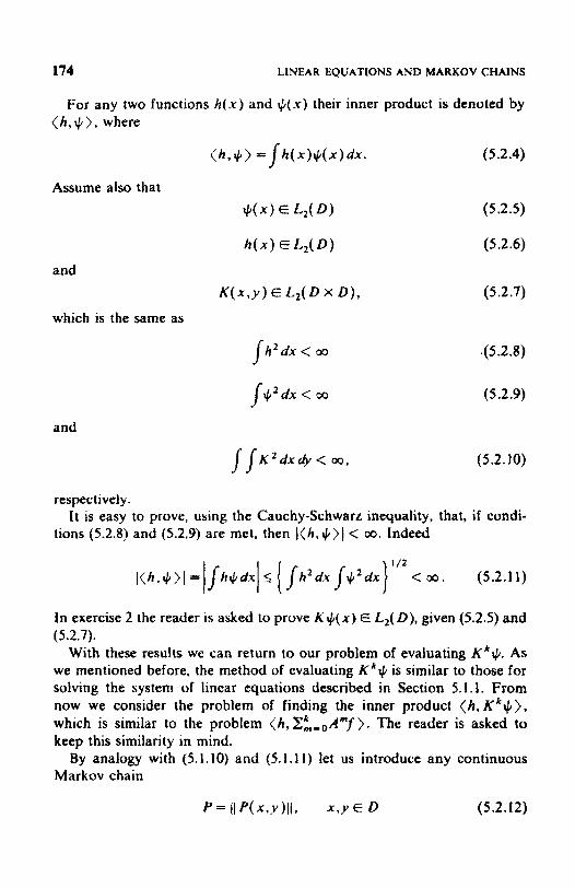
174 LINEAR EQUATIONS AND MARKOV CHAINS
For any two functions h ( x ) and $(x) their inner product is denoted by
( h , It> = j h ( x ) $ ( x ) dx. (5.2.4)
( h , $), where
(5.2.5)
(5.2.6)
(5.2.7)
j h ’ d x < 03 .(5.2.8)
JJ.’ dx < OQ (5.2.9)
and
S I K ’ d x i @ < 00, (5.2.10)
respectively.
tions (5.2.8) and (5.2.9) are met. then \ (h, +)I < co. lndeed It is easy to prove, using the Cauchy-Schwarz inequality, that, if condi-
In exercise 2 the reader is asked to prove K+(x ) E L2( D) , given (5.2.5) and (5.2.7).
With these results we can return to our problem of evaluating Kk+. As we mentioned before, the method o f evaluating K k $ is similar to those for solving the system of linear equations described in Section 5.1.1. From now we consider the problem of finding the inner product ( h , K k \ t ) , which is similar to the problem (h,ZL, ,A”’ f ) . The reader is asked to keep this similarity in mind.
By analogy with (5.1.10) and (5.1.11) let us introduce any continuous Markov chain

INTEGRAL EQUATIONS 175
satisfying jP(x,y)dy = 1, J p ( x ) d x = I , such that 1 p ( x ) > 0 , ifh(x)#O
2 P ( x , y ) > 0 if K ( x y ) + 0, (5.2.13)
where p ( x ) and P ( x , y ) are, respectively, the initial and the transition densities of the Markov chain (5.2.12)-(5.2.13).
By analogy with Proposition 5.1.1 we can readily prove the following
(5.2.14)
(5.2.15)
(5.2.16)
Assuming for some given y that h f x ) -p( .x) = 6(x -y), where a(,) is Dirac’s delta function, we immediately obtain E[q,(h)J = Kk+.
The procedure for estimating the inner product <h, K k f }, where K k # is defined in (5.2.3), can be written by analogy with the procedure for estimating ( h , d k + ’ ) ) in Section 5.1.1 as foIlows:
t Choose any integer k > 0. 2 Simulate N independent random paths x:)+x/’)-+. . - -+xp), s =
3 Find 1,2,. . . , N, from Markov chain (5.2.12)-(5.2.13).
(5.2.17) h ( x , )
P(X0) qy) (h )= -Wpqi (xk ) , s = 1 )..., N,
where
(5.2.18)
4 Calculate N
(5.2.19) I B k = - ~ $ ) ( h ) m ( h , K ~ \ t , ) ,
lv 2 - 1
which is an unbiased estimator of the inner product ( h , K k + ) .

1 76 LINEAR EQUATrONS AND MARKOV CHAINS
5.2.2 integral Equations of tbe Second Kind Consider the following integral equation of the second kind:
4 x 1 =I K(x,x,)dx,)dx, + . f ( x ) , (5.2.20) D
which can be written as
z = Kz +f. (5.2.2 1)
Let us assume that f ( x ) E L2( D), K ( x , x , ) E L2(D X D) , and
IX.I=suP~IK(x,Y)ldL< 1- (5.2.22)
Under these assumptions by analogy with (5.1.4) we can estimate (5.2.20), applying the following recursive equation:
Z(k+ 1) = Kt(k) + f. (5.2.23)
D
Setting Zo = 0 and KO =- 0, we get k
z '" ' ) -f+ Kf+ * * * + Kkf t C Kmf. (5.2.24) m - 0
Taking the limit k
lim d k ) = lim K m f = = z , k+w k - r m ,,,-a
we obtain the exact solution of z provided the von Neumann series converges.
One way of estimating ( h , ~ ) is via simulation of a continuous Markov chain similar to (5.1.10)- (5.1. I I).
The following proposition can be readily proved [8] by analogy with Proposition 5.1.1.
Proposition 5.2.2 For any given vector h
where the r.v. q k ( h ) is defined on the path xo+xI+* * + X k , such that

INTEGRAL EQUATlONS 177
The sample mean N k
(5.2.28)
estimates the inner product ( h , Z i _ o K ' " j ) .
an infinite path xo+xI +. - + x k + Assuming again h ( x ) = p ( x ) = S(x -y), we obtain (5.2.23). Considering
* , we define the random variable
(5.2.29)
It can be shown that for q,(h) to be an unbiased estimator of ( h , ~ ) , that is,
it is not enough to assume the convergence of the von Neumann series ZZ=&"f, that is,
00
2 K r n f < o o . (5.2.3 1) m=O
The reader is asked in exercise 5 to prove (5.2.301, provided
$j, f K m f l < o o . (5.2.32)
It is obvious that, when K ( x , y ) 2 0 andf(x) 2 0, both (5.2.31) and (5.2.32) coincide.
Another way of estimating ( h , z ) is via simulation of a continuous Markov chain with an absorbing state similar to that of (5.1.50)-(5.1.51). Consider the random path xo-+x, -+ - . . - + x ( ~ ) with the absorption time k, which is a random variable such that E ( k ) < m. Define on this path the r.v. (compare with (5.1.52))
m=O
(5.2.33)
where g( x) is the absorption probability, p ( x ) is the initial distribution, and
Then by analogy with Proposition 5.1.4 we can readily prove
E [ 7l,, ,(h)] = ( h , z ) , (5.3 35)
provided Ez-ol K m f l < co.

178 LINEAR EQUATIONS AND MARKOV CHAINS
To estimate ( h , z ) we simulate A' random paths x ~ ) + x ! ~ ) + * * - -+x(';\ with absorption state and find
(5.2.36)
The problem x = A x +j can be considered as a particular case of the problem z = Kz + f. Indeed, let us partition the region D into n mutually disjoint subregions Oil i = 1,2,. . . , n, such that D = and let us assume thatf(x) and K ( x , x , ) are constant functions in each subregion Di, i = 1,2,. . . ,n, that is,
f(x) = A ? x E Di
Qxrx,) =a, , , x E D,, x , E 0,. (5.2.37)
Then, for any x E Di, n
(5.2.38)
Inasmuch as z( x ) does not depend on x , the last formula can be written as
z i = C u,/z , + A * (5.2.39)
Thus by partitioning the region D into n disjoint subregions, we can find the solution of the integral equation (5.2.19) by solving the system of linear equation (5.2.39).
n
I" 1
5.23 Eigenvalw Robtern
Consider the following homogeneous integral equation:
Z ( X ) = hJK(x.x,)z(x,)dx,, (5.2.40)
which can be written as z=AKz. (5.2.4 I )
If z # 0, then X is called the eigenvalue and z ( x ) is called the eigenfunction corresponding to A.
Let us assume that the smallest eigenvalue A, is positive and that the ker- nel K( x , y ) = K ( y , x ) is symmetric and positive definite, that is, ( K + , +} > 0 if # 0. Under these assumptions for any two positive functionsf and
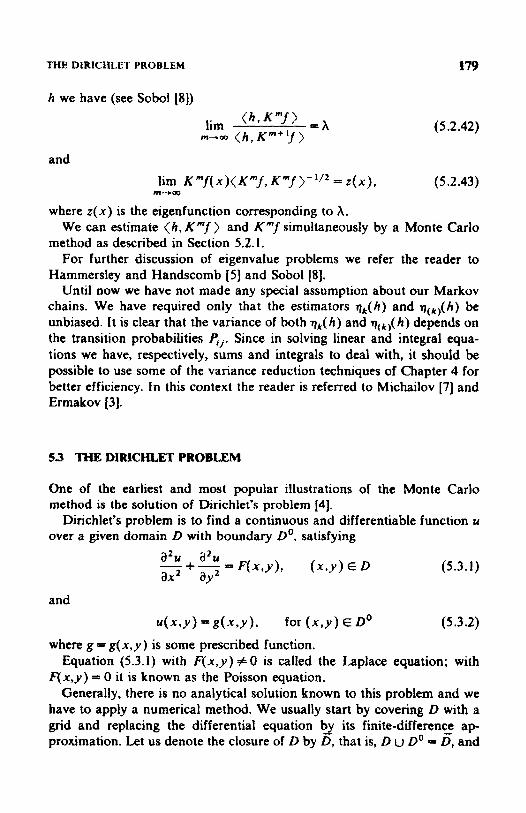
THE DIRICHLET PROBLEM 179
h we have (see Sob01 IS))
(5.2.42)
and
lim K m f ( x ) ( K m f , K" ' f>- ' /2 = t ( x ) , (5.2.43) m-cm
where z(x) is the eigenfunction corresponding to A. We can estimate ( h , K " j ) and K"f simultaneously by a Monte Carlo
method as described in Section 5.2. I . For further discussion of eigenvatue problems we refer the reader to
Hammersley and Handscomb [S j and Sobol[8]. Until now we have not made any special assumption about our Markov
chains. We have required only that the estimators qk(h) and ~ ( ~ ) ( h ) be unbiased. It is clear that the variance of both qk( h ) and qk,( h ) depends on the transition probabilities 4,. Since in solving linear and integral equa- tions we have, respectively, sums and integrals to deal with, it should be possible to use some of the variance reduction techniques of Chapter 4 for better efficiency. in this context the reader is referred to Michailov [7] and Ermakov 131.
53 THE DIRlCHtMT PROBLEM
One of the earliest and most popular illustrations of the Monte Carlo method is the solution of Dirichlet's problem 141.
Dirichlet's problem is to find a continuous and differentiable function u over a given domain D with boundary Do, satisfying
(5.3.1)
and
u ( x . y ) = g ( x , y ) . for ( X , Y E Do (5.3.2) where g = g ( x . y ) is some prescribed function.
Equation (5.3.1) with F(x ,y ) # 0 is d i e d the Laplace equation; with F ( x , y ) = 0 it is known as the Poisson equation.
Generally, there is no analytical soIution known to this problem and we have to apply a numerical method. We usually start by covering D with a grid and replacing the differential equation by its finite-difference a p proximation. Let us denote the closure of D by 5, that is, D u Do = 5, and

1%0 LINEAR EQUAHONS AND MARKOV CHAINS
the coordinates of the grid by x , = ah and y8 = ph, where h is the step size. Taking the two-dimensional case for convenience, we call the point ( x,,ya) E 5 an interior point of 6 if four neighbor points of (x,,yg), namely, - (x, - h a a ) , (x, + h,ya), (x,,up - h) , and (x,,y8 + h ) also belong to D.
We call ( x , , y p ) ~ D a boundary point if there are not four neighbor points that belong to 5.
'faking this definition into account, we have for any interior point
ua+ t , f i *'a@ + ' a - h,p ua . . f i+~ - *Ma8 + ua.B-1 i- E: Fa83 ( X , , Y ~ ) E D ,
(5.3.3) h2 h2
which is the finite-difference equation of (5.3.1). Here uOp = u(xa,ya), Faa = F(x,, x8), u,, = u(x, 2 h,yp), and u,,8-c = u(x,,yp2,) . The fast equation can be rewritten as
(5.3.4)
U 0 . p ga.8 and (x,+yp) E Do. (5.3.5)
% @ = f ( ~ , - I , p + U P + l . B + ~ , , p - 1 ~ 0 , / 3 + 1 - h 2 F p ) .
The boundary condition (5.3.2) is then
It is not difficult to see that by numbering all the points (x, ,y@) E B i n any order we can rewrite (5.3.4) and (5.3.5) as
n
u,= 2 u,,u,+x, i , j - 1 , 2 ,..., n. (5.3.6)
Here n is the number of mesh points f.x,,.v8) E 5, which is also equal to the order of the matrix Ii a,, / I ;.
The matrix [lu,,ll has a specific structure: all diagonal elements are equaI to zero; each row corresponding to an interior point of D has four elements equal to $, ail other elements being zero; each row corresponding to a boundary point of Do contains also elements equal to or zero, but the number of $ elements is as that of neighboring points, which is always less than 4.
Thus the Dirichlet problem is approximated by a system of linear equations (5.3.6), which can be solved by the Monte Carlo methods described in Section 5. I .3.
J - 1
EXERCISES
1 Describe an algorithm for simulating an ergodic Markov chain. 2 Prove that K $ ( x ) E Lz(D) , given (5.2.5) and (5.2.7).
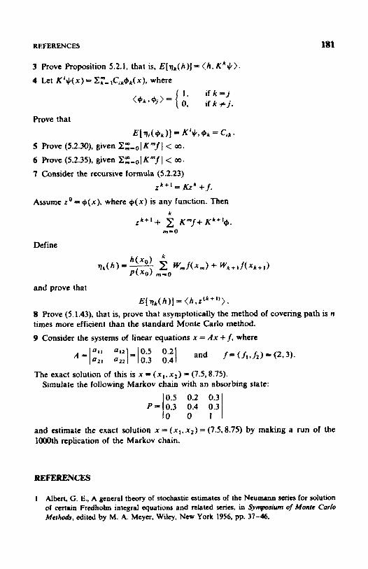
REFERENCES 181
Prove that
5 Prove (52.30). given Zz-ol K m j l < 03. 6 Prove (5.2.35), given x: , , lKmjl < 00. 7 Consider the recursive formula (5.2.23)
E [ q i ( + k I] ie K ' # > b k a Gin.
z k + I = K r k + + f .
Assume z o = +(x), where +(x) is any function. Then k
i r k + ' + K m f + Kk+'+ . m=O
Define k
2 w m f ( x m ) + wk+I/(xk+l) h(x-0)
V k ( h ) = - P ( X O ) m-0
and prove that
8 Prove (5.1.43), that is, prove that asymptotically the method of covering path is n times more efficient than the standard Monte Carlo method. 9 Consider the systems of linear equations x = Ax +f, where
E [ q k ( h ) ] = ( h , Z " + ' ) } .
The exact solution of this is x = (xl. x l ) = (7.58.75). Simulate the following Markov chain with an absorbing state:
0.5 0.2 0.3 P I 0 3 0.4 0 3
and estimate the exact solution x = (xI, x 2 ) = (7.5,8.75) by making a run of the IOOOlh replication of the Markov chain.
l o 0 I ' I
REFERENCES
I Albert, G. E., A general theory of stochastic estimates of (he Neumaan series for solution of certain Fredhdm integral equations and related series, in Symposium o/ Monre Carlo Merhodr, edited by M. A. Meyer. Wiley, New York 1956, pp. 37-46.

182 LINEAR EQUA’HONS AND MARKOV CHAINS
2 Cinch, E.. Infroducrion fo Stochatric P m m e s . Pnntice-hall. Eaglewood Cliffs. NCW Jersey, 1975.
3 Ennakov, J. M., Monte Cario Method and Related QuesfMN, Nauka, M m w , 1976 (ia Russian).
4 Forsythr, S. E. and R. A. Leibler, Matrix inversion by a Monte Carlo method, Math. Tables Other Aidr Compuf., 4, 1950, 127- 129.
5 Hammersky. I. M. and D. C. Handscomb. Morrtu CurloMeihnds. Illethuen. 1.ondon. 1964
6 Halton. 1. H.. A retrospective and prospective survey of Monte Carlo method, Soc. Xndurr. Appl. Math. Rev.. 12, 1970, I - 63.
7 Michaiiov, G. A., Some Problem in tho Theory of f h t Monre Cad0 Meihod, Nauka, Novosibirsk, U.S.S.R., 1974 (in Russian).
8 Sobol, J. M., Cmywtational Metltodr of Monfe Carlo. Nauka, Moscaw, 1973 (in Russian). 9 Spanicr. J. and E. M. Gclbard, Monre Carlo Principles and Neutron Tronsporta;im
Problem, Addison-Wesley, Reading, Massachusetts, 1969.

C H A P T E R 6
Regenerative Method for Simulation Analysis
6.1 INTRODUCTION
i t has already been mentioned in Chapter I that many real-world problems are too complex to be solved by analytical methods and that the most practical approach to their study is through simulation. In this chapter we consider simulation of a stochastic system, that is, of a system with random elements. Simulation of such systems can be considered as a statistical experiment, in which we seek valid statistical inferences about some unknown parameters associated with the output of the system (or the associated model) being simulated. However, classical methods of statistics are often unsuitable for estimating these parameters. The reason, as we see later, is that the observations made on the simulated system are highly correlated and nonstationary in time; under these circumstances it is difficult (actually impossible} to carry out adequate statistical analyses of the simulated data. To overcome these difficulties a procedure based on regenerative phenomena, called the regenerative method, has recently been developed.
Historically, Cox and Smith [4] were the first to suggest use of regenera- tive phenomena for simuiating a queueing system with Poisson arrivals. This idea was extended by Kabak [39] and Poliak 1591. Quite recently, Crane and Iglehart [6-91 developed a methodology for the regenerative method, based on a unified approach to analyze the output of simulations of those systems that have the property of self-regeneration, that is, of invariably returning (at particular times) to the conditions under which the future of the simulation becomes a probabilistic replica of its past. In other words, if the simulation output is viewed as a stochastic process, the
183
Simulation and the Monte Carlo Method R E W E N Y. RUBINSTEIN
Copyright 0 1981 by John Wiley & Sons, Inc.

184 REOENERATIVE METHOD FOR SIMULATION ANALYSIS
regenerative property means that at those particular times the future behavior of the process is independent of its past behavior, and is governed by the same probability law, that is, at those times the stochastic process “starts afresh probabilistically.” Crane and iglehart showed that a wide variety of problems, such as communication networks, queues, main- tenance and inventory control systems, can be cast into a common framework using regenerative phenomena; they then proposed a simple technique for obtaining point estimators and confidence intervals for parameters associated with the simulation output.
The regenerative method also provides answers to the following im- portant problems: how and when to start the simulation, how long to run it, when to begin collecting data, and how to deal with highly correlated data.
The theory and practice of the regenerative method are now in the process of rapid development. The list of references contains about 100 relevant papers known to the author. An excellent introduction to the regenerative method can be found in Crane and Lemoine’s book (101. Iglehart’s forthcoming monograph 138) will present a rigorous development of both the theory and practice. Many others recently obtained results, in particular regarding simulation of response time in networks of queues, are to be found in lglehart and Shedler’s monograph [37].
This chapter is organized as foliows. The basic ideas of the regenerative method are discussed in Section 6.2. Section 6.3 deals with statistical problems, in particular with the confidence interval for the expected values of some functions defined on the steady-state distribution of the process being simulated. In Section 6.4 the ideas of the regenerative method are illustrated for a single-server queue, a repairman system, and a closed queueing system. Choice of the best among a set of competing systems is the subject of Section 6.5. Section 6.6 deals with a linear programming problem in which the coefficients are unknown and presents the output parameters of regenerative processes. Variance reduction techniques in regenerative simulation are the subject of Section 6.7.
6.2 REGENERATIVE SlMUWTiON
We start this section with the definition of a regenerative process. Roughly speaking, a stochastic process ( X ( f ) : I 2. 0) is called regenerative if there exist certain random times 0 < To < T, < T, < * - - forming a renewal process’ such that at each such time the future of the process becomes a
*A sequence of random variables (q : n 2 0) is a renewal 6 provided !hat To = 0 and T, - Ta-, (n 2 1) are i.i.d. r.v.’s.

6.2 REGENERATIVE SIMULATION 185
probabilistic replica of the process itself. Informally, this means that at these times the future behavior of the process is independent of its past behavior and is invariably governed by the same law. In other words, the part of the process ( X ( r ) : T i - , < f I T,} defined between any pair of successive times is a statistically independent probabilistic replica of any other part of the same process defined between any other pair of successive times.
The times {T : i 2 0) are called regeneration times and the time between q - , and T, is referred to as the length of the ith cycle. Formally [5 ] , a stochastic process ( X ( t ) : f 2 0) is regenerative if there exists a sequence To, T,, . . . of stopping times+ such that:
I T = { q : I = O , l , . . . I isarenewalprocess. 2 For any I , rn E (0, 1 , . . . I , f,, . . . , i , > 0, the random vectors
( X ( r , ) , . . . , X ( t , ) } and (X(T, + t , ) , . . . .X(T, + r , } are identically distrib- uted and the processes (X(f) : t < T,} and (XCT, f I ) : f 2 0 ) are indepen- dent.
For example, let { X, : n 2 0) be an irreducible, aperiodic, and positive recurrent Markov chain with a countable state space I 5 (0, I , . . . }, and let j be a fixed state; then every time at which statej is entered is a time of regeneration.
Let us select a fixed state of the Markov chain (M.C.), say state 0. We then obtain a sequence of stopping times { q : i 2 0) such that O = To < T, < T2 < . - and X, - 0 almost surely (as.); that is, once the system enters state 0, the simulation can proceed without any knowledge of its past history.
For another example, let us consider the queue size at time t for a Gi/G/ 1 queueing system. Suppose the time origin is taken to be an instant of departure at which rime the departing customer leaves behind exactlyj customers. Then every time a departure occurs leaving behindj customers, the future of the stochastic process after such a time obeys exactly the same probability law as when the process started at time zero. More examples of regenerative processes are considered in Section 6.4.
I t is shown in Ref. 8 that under certain mild regularity conditions the process ( X ( t ) : I > 0 ) has a limiting steady-state distribution in the sense that there exists a random vector X such that
lim P{ X ( r ) 5 x} = P( X 5 x). I-+W
.A random variable T taking values in [O, + , OD) is a stopping time [S) for a stochastic process { X ( r ) : r 2 O), provided that for every finite f 2 0, the occurrence OT nonoccurrence of the event {T 5 r ) can be determined from the history ( X ( s ) : s c t ) of the process up to time 1.
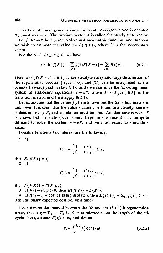
186 REGENERA1 1VE METHOD FOR SIMULATION ANALYSIS
This type of convergence is known as weak convergence and is denoted X(r)rjX as r + 00. The random vector X is called the steady-state vector.
Let f : Rk-+ R be a given real-valued measurable function, and suppose we wish to estimate the value r = E { f ( X ) } , where X is the steady-state vector.
For the M.C. {X,, : n 2 0 ) we have
r = ~ ( f ( ~ ) ) = z f ( i ) P ( X = i ) - x j ( i ) q . (6.2.1) i E I i E I
Here, n = ( P ( X = i ) : i E I} is the steady-state (stationary) distribution of the regenerative process { X,, : n > 0}, and f ( i ) can be interpreted as the penalty (reward) paid in state i. To find r we can solve the following linear system of stationary equations, n = nP, where P = (el : i, j E I ) is the transition matrix, and then apply (6.2. I).
Let us assume that the valuesf(i) are known but the transition matrix is unknown. It is clear that the value r cannot be found analytically, since 7~
is determined by P, and simulation must be used. Another case is when P is known but the state space is very large; in this case it may be quite difficult to solve the system n*sP, and we must resort to sirnulation again.
Possible functions f of interest are the following:
1 If
then E ( f ( X ) ) = 9, 2 If
then E ( f ( X ) } = P ( X l j } . 3 Iff(i)==iP,p>O, then E { f ( X ) ) = E { X P } . 4 If f ( i ) = c, = cost of being in state i, then E ( f ( A')} - &,c, P( X = i )
(the stationary expected cost per unit time).
Let 5 denote the interval between the ith and the (i + 1)th regeneration times, that is 7 = q+ - 7;, i 2 0; 7, is referred to as the length of the ith cycle. Next, assume E(T,) < 00, and define
(6.2.2)

6.3 POINT ESTIMATORS AND CONFIDENCE lNTERVALS 187
or T , + , - l
(6.2.3)
depending on whether the process ( X ( t ) : t 2 O} is continuous-time or discrete-time. In other words, y. is the penalty (reward) during the cycle of length T~ = q+ , - q.. Naturally, Y, is a random variable (r.v.) because so are T, and f( Xi) .
We now formulate two fundamental propositions that are used exten- sively in the rest of this chapter.
Proposition 6.2.1. The sequence {( T , T ~ ) : i 2 I } consists of independent and identicaily distributed (i.i.d) random vectors.
Propitioo 6.2.2. I f T , is aperiodic,* E ( r l ) < og, and E ( l f ( X ) l ] < 00, then
(6.2.4)
There is an analogous ratio formula when T ! is periodic. For proof of these propositions the reader is referred to [S].
Proposition 6.2.1 says that the behavior patterns of the system during different cycles are statistically independent and identically distributed. Proposition 6.2.2. enables us to estimate the value r = E( Y , ) / E ( 7 , ) (which is the same as r = E( Y , ) /E( 7, ) ) by classical statistical methods, and to find point estimators and confidence intervals fur r. These two problems are the subject of the next section.
63 POINT ESTIMATORS AND CONFIDENCE LlVTERVAI.23 [tZ, 281
In this section we consider several point estimators and confidence inter- vals for the ratio E ( Y , ) / E ( 7 , ) . The problem we consider is as follows: given the Lid. sequence of random vectors { ( Y , T ~ ) : ~ > l}, find point estimators and construct IOO(1 - &)% confidence intervals for the ratio E( r, )lQ 7, 1.
*The random variable T, is periodic with period X > 0 if, with probability 1, it assumes values in the set (0, A, 2X,. . . ] and A is the largest such number. if there is no sucb A, then T , is said to be aperiodic.

188 REGENERATIVE METHOD FOR SIML%ATION ANALYSIS
Let Z, = Y, - '7,. It is readily seen that the Z,'s are i.i.d. r.v.'s, since the vectors (Y,, 7,) also are. Note also that
E ( Z , ) = 0 (6.3.1)
and a Z = v a r ( Z , ) = v a r ( Y , ) - 2 r c o v ( Y , , ~ , ) f r 2 v a r ( ~ , ) . (6.3.2)
Denote Y = (1 /n)X;, I Y,, and 7' = (1 / n ) z : , fr ,; then by virtue of the central limit theorem, (c.1.t.) we have
(6.3.3)
where 3 denotes weak convergence and it is assumed that o2 < 00. The last formula can be rewritten as
(6i3.4)
where i = F/+. Inasmuch as u is unknown, we cannot obtain a confidence interval for r directly from (63.4). However, we can estimate u2 in (6.3.2) from the sample, that is, by
s2 =si, - 2 i s 1 , + f 2 s z z , (6.3.5)
where
and . n
It is straightforward to see that s 2 - w 2 a.s. as n+w, so (6.3.4) can be rewritten as
n"2( i - r ) S/ .F
e N ( 0 , I}, as n-w,
and the I O O ( 1 - 61% confidence interval for r = E( ~ ) / E ( T ~ ) is
(6.3.6)
(6.3.7)
where t6 = (p- '(I - S/2), $J is the standard normal distribution function, and i = y/F is the point estimator of E ( Y l ) / E ( T i ) . The procedure for
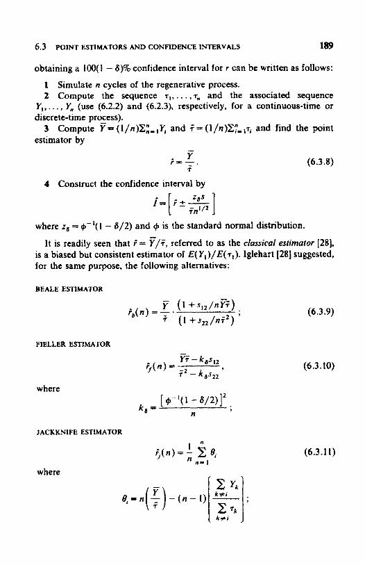
6.3 POINT ESTIMATORS AND CONFIDENCE INTERVALS 189
obtaining a loo( 1 - a)% confidence interval for I can be written as follows:
1 2 Compute the sequence . . . ,rn and the associated sequence
Simulate n cycles of the regenerative process.
Y, ,..., Y, (use (6.2.2) and f6.2.3), respectively, for a discrete-time process).
3 Compute Y=(l/n)Z:,,Y, and 7’ ( l /n)xy-i7i estimator by
- Y i = y . 7
continuous-time or
and find the point
(6.3.8)
4 Construct the confidence interval by
where zd = +-‘(I - 6/2) and + is the standard normal distribution.
It is readily seen that i- = T/F, referred to as the clarsicul estimator [28], is a biased but consistent estimator of E( Y , ) / E ( T ~ ) . Iglehart [28] suggested, for the same purpose, the following alternatives:
BEALE ESTIMATOR
FIELLER ESTIMATOR
where
JACKKNIFE ESnMATOR
where
(6.3.9)
(6.3.10)
(6.3.11)

190 REGENERATIVE METHOD FOR SIMULATION ANALYSIS
TIN ESTlMATOR
(6.3.12)
Let us now cite some results from Ref, 28. The four point estimators (6.3.9) through (6.3.12) as well as the classical estimator are biased. Their expected value can be expressed as
E [ i (n) -J 5= r + c + 2 c2 + o( f ) (6.3.1 3)
The point estimators (6.3.9), (6.3.1 l), and (6.3.12) have been suggested in order to reduce the bias of (6.3.13) up to order I / n 2 . For the jackknife method c , = 0, since
The reader is asked to prove that for both Beale and Tin estimators c , / n is also equal to zero.
- i,}--+O as. as n 3 ~ , we can replace i both in (6.3.6) for the c.1.t. and (6.3.7) for the confidence interval without changing the results.
For the jackknife method formulas (6.3.6) and (6.3.7) can be written, respectively, as
Since both n ’ / * ( i - i b b ) d O and
9 - r
i * N ( O , 1) as n-+ 00
/ 2 $ (6.3.14)
where
The FielIer method yields the following lOO(1 - 6)% confidence interval:
(6.3.15) 0 ’ / 2
I,= 7 - 7 t, + I- ( 7 2 - k,szz ) ( i2 - k,s,,)

6.3 POINT ESTIMATORS AND CONFIDENCE INTERVALS 191
where
and
[ + - ‘ ( I -w]’ k, = n
The performances of these estimators were compared numerically (via simulating several stochastic models), and the following results were ob- tained [28].
For short runs the jackknife method is recommended both for point estimators and confidence intervals because it produces slightly better statistical results than other methods. Two minor drawbacks of the jack- knife method are a large memory requirement and slightly more complex programming. Additional storage addresses of the order of 2n are required, where n is the number of cycles observed. Where the storage requirement for the jackknife method is excessive, the Beale or Tin methods are recommended for point estimates and the classical method for the confi- dence intervals. The Fieller method is recornmended for neither point nor confidence intervals. It is found to be heavily biased for short runs and more compiicated than the classical method. The above mentioned five point estimators were based on simulating n cycles of regenerative processes. Another possibility is to consider point estimators based on the simulation for a fixed (but large) Length of time f . In this case the number of cycles N, in the interval (0, r ] is a random variable given by
N, = 2 $ o , q K l s= 1
where I,o,rl is the indicator function of the interval [O, t j . Replacing n by N,, we can modify all the point estimators (6.3.8) through (6.3.12), preserv- ing their consistency. For example, for the classical estimator we have
Thus, asymptotically, there is little difference while considering point estimators based on simulation n regenerative cycles or on simulation for fixed length of time 1. The c.1.t. in this case is

192 REGENERATIVE METHOD FOR SiMULAnON ANALYSIS
Recently Heidelberger and Meketon 1321 considered estimators based on simulations for a relatively short length of time I . They defined estimators
Nt
i = I x x
i( N,) = - X Ti
i - I
(6.3.17) *v,
and N, + 1
They then showed that
E f i ( N,)) = r + O( L ) 1 .
(6.3.18)
(6.3.19)
and
E ( i ( N , + l ) ) = r + o ( + ) , (6.3.20)
so that a bias reduction is achieved by continuing the simulation until the first regeneration after time r. The bias reduction is comparable to that of the jackknife, Beale, and tin estimators since t is proportional to the number of cycles. Table 6.4.3 lists empirical results from simulations of a closed queueing network model for these estimators.
We turn now to the problem of determining run length. The lOO(1 - S)% confidence interval for a large but fixed number of cycles has a width approximately equal to
2a+- ’( I - 6/2) - E ( T , ) n ’ / 2 ’
In terms of duration time I (6.3.20) can be written as (see [24])
(6.3.21)
(6.3.22)
Note that neither u nor E ( 7 , ) are known in advance. Hence it may be worthwhile to take a small sample and obtain rough estimates for u and E(T,) . Such estimates would form a basis for a final decision or run length

6.4 EXAMPLES OF REGENERATIVE PROCESSES 193
and level of confidence. We wish to emphasize that all ratio estimators described in this section are designed for simulations with a fixed number of cycles n or a fixed run length t. An alternative possibility would be to consider procedures based on sequential stopping rules.
6.4 EXAMPLES OF REGENERATIVE PROCESSES
In this section we consider three examples of regenerative processes, taken from Refs. 6, 10, and 49: a single server queue, a repair model with spares, and a closed queueing network.
6.4.1 A Single Server Queue GI/G/Z [ti]
This example was described in Section 4.3.12, and will be briefly recapitulated here.
Let Cr: and S, be the waiting time and service time, respectively, of the ith customer in a singe server queue. Let A,+, be the time between the arrival of the ith and ( i + 1)th customers. We assume that {S,, i 2 0) are i.i.d. with E ( 8 ) = p-' and that { A , , i 2 I } are i.i,d. with .!?(A,) = A - ' , Let the traffic intensity p be defined by p = A/p. We assume that customer number 0 arrives at time 0 to an empty system. Let X, = S,- I - A , for i 1 1. The waiting time process {W,, i 2 0) can be defined recursively by
w,-0
~ = ( F V , - ~ + X , ) + , i > I .
It i s known [36] that, if p < 1, there exists an infinite number of indices i such that W, 3: 0 and a random variable W such that W,* W, as i 4 to. Thus we choose zero state as our return state and regenerations occur whenever a customer arrives to find an empty queue. We are interested in estimating E ( W ) , which is finite if E(S:) < m.
Since no analytical results are available for calculating the steady-state waiting time E ( W ) , we estimate it via simulation by making use of the classical estimator (6.3.8). The simulation results are shown in Fig. 6.4.1,
We see that the customers I , 3,4, 7, 11, and 16 find the server idle, that is, W, = W, = W, = W, = W , , = W,, = 0, while customers 2, 5, 6, 8, 9, 10,. 12, 13, 14, and 15 find the server busy and wait in the queue before being SC?fVed.
It follows from Fig. 6.4.1 that the simulation data contains five complete cycles with the following pairs {(&7,) , i = 1,. . . , 5 ) : (Y1,71) (10,2),
The sixth cycle will start with the arrival of customer 16. Using the ( Yz, r2) = (0, l), (Y,, T ~ ) = (30,3), (Y,, 7,) = (50,4), and ( Y5, T5) = (60 ,5) } -
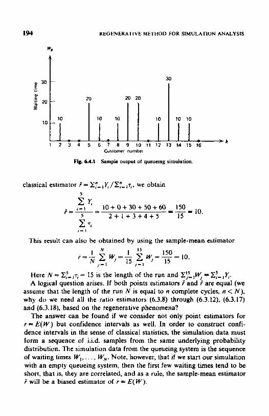
194 REGENERA I IVE METHOD FOR SIMULATION ANALYSIS
Customer number
Fig. 6.4.1 Sample output of queueing simulation.
classical estimator i = 2:= ,x /Z;- , T ~ , we obtain
i K , - I 10+0+30+50+60 150 r = - - - =-* 10.
5 2 + 1 + 3 + 4 + 5 15 2 7,
1 - 1
This result can also be obtained by using the sample-mean estimator
l N I l 5 150 15 i=- wj=Ts 2 w,=-=10. ,-, 1-1
Here N = C:-,T, = 15 is the length of the run and Zy-tW, = C:-,q. A logical question arises. If both points estimators r' and F are equal (we
assume that the length of the run N is equal to n complete cycles, n < N), why do we need all the ratio estimators (6.3.8) through (6.3.12), (6.3.17) and (6.3.181, based on the regenerative phenomena?
The answer can be found if we consider not only point estimators for r = E( W ) but confidence intervals as well. In order to construct confi- dence intervals in the sense of classical statistics, the simulation data must form a sequence of i.i.d. samples from the same underlying probability distribution. The simulation data from the queueing system is the sequence of waiting times W,, . . . , W,. Note, however, that if we start our simulation with an empty queueing system, then the first few waiting times tend to be short, that is, they are correlated, and as a rule, the sample-mean estimator ? will be a biased estimator of r = E( W).

6.4 EXAMPLES OF REGENERATIVE PROCESSES 195
Tabie 6.4.1. Simulation R d t s for tbe M / M / t Queue
Parameter Value Point Estimates Confidence Interval Theoretical
0. loo 0.110 [0.0%,0.123] E( y, ) r = E( W ) = - E( 7 , )
&W2) + 0.040 0.046 [0.035,0.056]
qfiw-:-oTj- } 0.120 0.133 [0.116,0.148] &7i) 2 .Ooo 2.1 10 [2.012,2.207] 4 W ) 0. I73 0.182 [0.141,0.271]
Source: Ref. 6. Note: Number of cycles n = Moo, level of confidence IOO(1 - 6) = 90%~ number of replications N = 10. h = 5, p = 10).
To overcome this difficulty we can run the model until it reaches the steady state and then start collecting and updating the simulation data. The problem of determining the steady-state distribution is a difficult one, moreover, requiring considerable computation (CPU) time, but unless we start from it W, and Wj+ , will again be correlated (if Wi is short, then W,+, will also tend to be short and vice versa). Since the r.v.'s W,, . . . , W, are correiated, classical statistical methods cannot be applied in constructing confidence intends for r = E( W ). Still, this difficulty can be overcome by using the regenerative property, namely, by grouping the simulation data into independent pairs (blocks) ( V,, 7, ) . . . . , ( Y,, T"), which yields different ratio estimators (see (6.3.8) through (6.3.12)' (6.3.17) and (6.3.18)) and the associated confidence intervals by means of classical statistics. Table 6.4.1 presents simulation results for the queueing system M/M/ I with h = 5, p = 10 based on a run of 2000 cycles. Confidence intervals at the 90% level are given for the parameters E( W ) , E( W 2 ) , E((V%'- 0.1 )+}, E ( T , ) , and a ( W ) . The function E ( d G I 7 +) may be interpreted as a penalty for long waiting time.
_I-.
6.4.2. A Repairman Model with Spares [lo]
We now consider a repairman problem with n operating units and M
spares (Fig. 6.4.2). Each of the operating units fails with rate A. A failed unit enters a queue for service from one of s repairmen on a first-in-first-out (FIFO) basis and is replaced by a spare (if available). The distribution of the i.i.d. repair times is exponential with mean p-' for each repairman. A
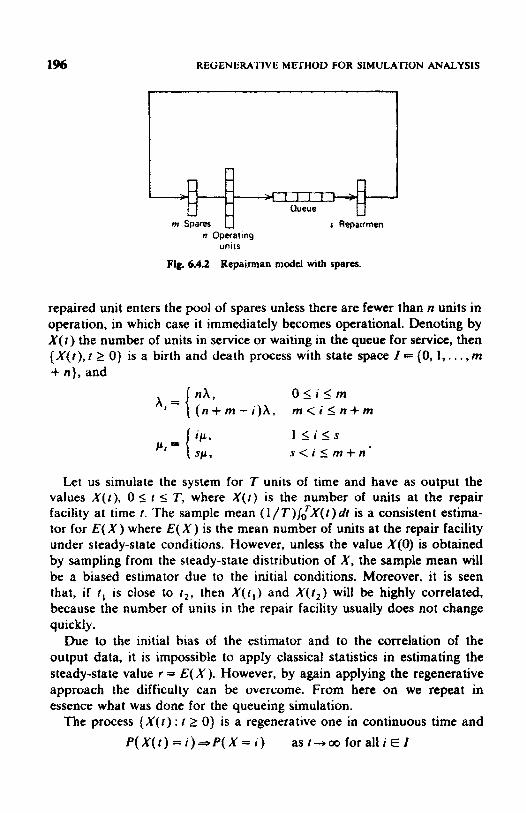
1% REGENERATIVE METHOD FOR SIMULA'NON ANALYSIS
& Queue
m Spares u r Repairmen n Operating
units
Repairman model with spares. Flg, 6.4.2
repaired unit enters the pool of spares unless there are fewer than n units in operation, in which case it immediately becomes operational. Denoting by X ( r ) the number of units in service or waiting in the queue for service, then { X ( t ) , r 2 0) is a birth and death process with state space Z = (0, 1,. . . , m + n ) , and
O l i < m m < i I n + m
I l i l s
A , = ( n h y ( n + m - i ) A ,
s < i 5 m + n
Let us simulate the system for T units of time and have as output the values X ( r ) , 0 5 I 6 T. where X ( r ) is the number of units at the repair facility at time r . 'The sample mean (l/T)j:X(t)dt is a consistent estima- tor for E( X ) where E( X ) is the mean number of units at the repair facility under steady-state conditions. However, unless the vaiue X ( 0 ) is obtained by sampling from the steady-state distribution of X, the sample mean will be a biased estimator due to the initial conditions. Moreover, it is seen that, if I , is close to r 2 , then X ( r , ) and X ( t z ) will be highly correlated, because the number of units in the repair facility usually does not change quickly.
Due to the initial bias of the estimator and to the correlation of the output data, it is impossible to apply classical statistics in estimating the steady-state value r = €( X). However, by again applying the regenerative approach the difficulty can be overcome. From here on we repeat in essence what was done for the queueing simulation.
The process { X( t ) : t 2 0) is a regenerative one in continuous time and P ( X ( r ) = i )=aP( X = i ) as t + 00 for all i E I

6.4 EXAMPLES OF REGENERATIVE PROCESSES 197
Table 6.4.2. Simulation Results for R e p o l h m ~ Model Parameter Theoretical Value Confidence Interval
5.353 (5.238,5.432] 1.269 [ I .201, 1.3251 0.465 [0.444,0.475] 0.988 [0.987,0.990] 0.012 [O.OIO, 0.013)
42.02 I i37.459.47.681 j 73.375 [65.262,83.342]
Source: Ref. 10. Note: Run length = 500 cycles; level of confidence - 95%.
Suppose we start the simulation at time TI = 0 with n operating units and M spares, that is, at T, = 0 the repair facility is empty; then the sequence is (7; : i 2 0}, where T. is defined as the regeneration time when the repair facility becomes empty. In other words, the system “starts afresh probabilistically,” or regenerates itself, at each time q. For any real-valued measurable function -f we define
then the pairs (Yt,7!), . . . ,( Y,,,7,). where ri = I;.+, - T,, are i.i.d. Suppose that the simulation time T exactly equals n cycles; then
D l . n
i- i
is a biased but consistent estimator for r = E ( f ( X ) ) = E ( Y , ) / E ( T ~ ) . Table 6.4.2 gives simulation results for some output parameters based on
run of 500 cycles. E ( i , ) represents the number of failures over a cycle. It is assumed that n = 10, m = 5, s = 4, and p = 2. The “lifetime” of an operat- ing unit is exponentially distributed with A = 5.
6.43 A Closed Qwueiag Network I491
Consider a closed queueing system that is a model of the time-sharing computer system in Fig. 6.4.3. The network comprises M service centers with a fixed number N of customers. Service center 1 consists of N

198 REGENERATIVE METHOD FOR SIMULATION ANAL.YSIS
i Fig. 6 4 3
terminals (identical parallel servers); hence a customer at this center never has to wait for a sewer to become free. Service center 2 is a single server processor, that is, all customers receive service immediately, and if there are k customers present each customer is served at I / & of the server’s rate. Service centers 3,. . , , M represent peripheral input-output devices (single server queues}, each of which is scheduled on a FIFO basis. A customer (device) completing service at service center 1 immediately enters service center 2, and immediately thereafter service center j with probability p, > 0, j = 3,. , . , M, where Z K 3 p , = 1. After completing service at service centerj , j = 3,. . . , M, the customer enters service center I with probability I - p . or service center 2 with probabilityp. Service times at service centers j = 1,2,. . . , M are i.i.d. and exponentially distributed with mean p,-’. It is assumed that routing through the network i s Markovian and that all service and routing mechanisms are mutually independent.
Let Q ( f ) = (Q , ( t ) , . . . , Q,,,(f)), where Q, ( f ) is the number of customers at service centerj at time 1. It can then be shown [49] that { Q ( r ) : f 2 0) is a continuous-time irreducible Markov chain, and hence a regenerative process. We define a response time as the time interval between a customer’s departure from service center I and his next return to it, and let W; be the just completed time of the i th customer arriving there. Then W = { W,, i 2 0 ) is regenerative with regeneration occurring whenever a last customer arrives at service center 1 leaving centers 2,. . . , M empty. Again, we are interested in the expected stationary response time r = E( W), which is known to be finite [49]. Let d, be the utilization of service center i, that is, the long run average proportion of time the server there is busy. The particular parameters chosen for this model are listed in Fig. 6.4.3 and yield d2 =: 0.894, d , = 0.268, r = 8.65.
Table 6.4.3 presents point estimators and 90% confidence intervals for several ratio estimators discussed in Section 6.4.3.

6.5 SELECTING THE REST STABLE STOCHASTIC SYSI'EM 199
TABLE 6.43. Point Estimates and 90 Confidence Intervals for E( W ) = 8.65 in C W Oueulne Network
N - 5 N = 10 N - 30 N = 50 Estimate 2 = 220 2 - 4 4 0 t = = 1320 t - 2220
i( 4 1 8.28 5 0.10
i( Nt + 1) 8.64 5 0.10
Classical i 8.23 +- 0.17
Jackknife 8.93 t 0.23
8.46 8.55 5 0.07 & 0.07
8.60 8.62 2 0.07 2 0.07
8.50 8.56 lr. 0.09 t 0.07
8.71 8.61 t 0.09 & 0.07
8.59 t 0.07
8.63 -e 0.07
8.60 rt 0.08
8.62 -c 0.08
Source: Ref.22. Note: N - number of cycles simulated; r = number of response times simulated; R = 200 repIications for t = 220, 440; R = 100 replications for t = 1320; R 60 replications for r = 2200.
65 SELECTING THE BEST STABLE SIOCHASTIC SYSTEM
In this section we consider some techniques for selecting the best system from among m alternative systems according to a certain criteria.
Assume that N( N 2 2) stochastic systems are being simulated, each giving rise to a regenerative process { X I ( f ) : t 2 0). i = 1,. . . , N. For exam- pie, N alternative designs are considered for a new system.
Suppose that the measure of performance for the ith system is
r , = E { f ( X ' ) ) , i = I ,..., N (6.5.1)
wherejis a real-valued bounded measurable function, X ' is the steady-state random variable of the regenerative process ( X ' ( t ) : f 2 0). The problem is to choose the best system, that is, the system with the smallest value of 5 :
r l - min r,= min E ( ~ ( X ' ) ) ) . (6.5.2) 1 - 1 ,_. . , N I = I ,..., N
(We are minimizing 5 ; the alternative problem of maximizing ri can be considered as well.)
Iglehart (301 presents a method based on the following scheme. Two positive numbers P* and S* are specified. Then with probability P* the system with the smallest (largest) r, is selected whenever that value of 5 is separated by at least P from the other 5's. Two procedures have been considered in Ref. 30 for this problem. The first procedure is sequential and the second is two-stage. Both procedures involve the use of normal

200 REGENERATIVE METHOD FOR SIMULATION ANALYSIS
approximations and require large samples in terms of the number of cycles of the regenerative processes simulated.
We consider here another adaptive approach suggested by Rubinstein (611. Our method is based on an iterative procedure that selects the best system with probability 1.
We start solving the problem (6.5.2) by considering the following linear programming problem:
N
min W( p ) = min C E{ j( x')}p,, (6.5.3) P p / = I
subject to N x p , = 1 , p , 2 0 , i = I ...., N. (6.5.4)
If there exists a unique solution of (6.5.2), then the problem (6.5.3)-(6.5.4) is equivalent to (6.5.2) and its solution is given by a vectorp* with a single nonzero component:
p* = (0 ,...) 0,1,0, ..., 0). (6.5.5)
f - 1
- I
The algorithm for solving the problem (6.5.3)-(6.5.4) is based on a step-by-step correction of the probability vector pin], where n denotes the step number. There exists a mechanism, provided by (6.5.9) below, which ensures that p,[n] 2 4n], i = I , . . . . N, where { ~ [ n ] } : - ~ is a monotone decreasing sequence of positive numbers, subject to (6.5.13) and (65.14) below. On the nth step the ith system, i E ( 1 , . . .,h'}, is chosen by simulating the distribution p [ n - I]. We denote this event by X [ n ) = X'. One cycle of the process { X ' ( r ) : I 2 0 ) is carried out. Denote by ~ ' [ n ] , i = I , . . . , n, the totai number of renewal cycles made by the ith system up to and including the nth step. We check whether or not the inequality v k [ n - I ] 2 ne[n] , k E { I , . . . , i - 1, i + I , . . + , N) is satisfied for all systems. If for some indices k , , . . . , k , E { 1, . . * , i - I, i + I,. . . , N}, this inequality does not hold then one additional cycle is carried out for each system k , , . . . , k, , so that ultimately
v k [ n ] 2 n e [ n l , k - I ,..., N. (6.5.6) We record
k 7," = qitml - 7&- 1' k = i , k , , . . . , k,,
the lengths of the cycles performed, and for each k calculate
j( X k ( i ) ) d r , k = i , k , , . . . . k , (6.5.7)
if the process { X ' ( t ) : i 1 0) is continuous-time.

6.5 SELECTING 'THE BEST STABLE STOCHASTIC SYSTEM 20 1
In the case of a discrete-time process the integral should be replaced by
(6.5.8)
We construct a new distribution p [ n ] by the following recurrence for-
A n 1 = % * , m , { P [ n - 11 - v b I H n l i ) ) . (6.5.9)
the corresponding sum over the v k [ n]th cycle. Set also Y," s= T," = 0, if k B { i , k l , . . . , ks}.
mula:
Here S, is a simplex in R N :
ns, is the projection operator onto the simplex S,, such that, for any x E R N ,
I l l -&)I! = min llz -yII, Y E S .
and B ( . I . ) is a vector { B , ( . l . ) ,..., B,( .I . ) ) , where
B k ( n l i ) ' ikp,'[ - ' I r k [ '1 (6.5.10)
(6.5.1 1)
Yk[n] = Y k [ n - I ] + Y,", # [ n ] = . ~ ~ [ n - I ] +T,k. k- I , ..., N (6.5.12)
The initial values of p[O] E ScIol, Y [O] = ( Y '[O], . . . , Y "O]), and 7[0] = ( ~ ' [ o j , . . . , T ~ [ O ] ) can be chosen arbitrarily, for example, Yk(0) = 0, ~ ~ ( 0 ) = 0, k = 1,. . . , N. The sequences { y [ n ] } r , and { ~ [ n ] ) , " ~ must be chosen so that the following conditions are satisfied:
(6.5.13)
(6.5.14)
(6.5.1 5)
m c dn1 c 00. (6.5.16) n=1 e [ n ] V i

202 REGENERATIVE METHOD FOR SIMULATION A N U Y S I S
Remark f example,
In order to satisfy conditions (6.5.13) through (4.5.16) take, for
y [ n ] - n - I , e [ n ] -11-0.4.
Remark 2 We assume that r," 2 r,, > 0, k = I , . . . , m, n = 1,2,. . . , that is, that the cycle is taken into account only if it is of some minimal length (which can be considered as the sensitivity threshold of the measuring instrument).
Remark 3 The r.v.'s Y k [ n ] and ~ ' [ n b k = 1 ,..., N, n l 1, defined in (6.5.12), store the information obtained up to and including the nth step. We should aIso note that, for each k fixed, only v L [ n ] summands in both Y k ( n ] and 7 ' [n l are nonzero.
Theorem 6.5.1 If the values of the function f are uniformly bounded by some constant D and if there exists the unique optimal solutionp* of the problem (6.5.3)-(6.5.4), then for any initial distribution p[O] E the sequence ( p [ n 11,"- ,, generated by the algorithm (6.5.9)-(6.5.14), converges t o p * with probability I .
Coroliary The theorem remains valid if we assume that the values of the function f cannot be observed directly, but are measured with a random noise. In other words,
!( x ' } = E ~ ( Q ( X',<)} , i = I . . . ., N, where 6 is a random vector with an unknown time-independent probability distribution function. In this case we can consider another random pro- cess:
{ U l ( t ) : i L ~ } = { ( x l ( r ) , t ) ) ; i = i ,..., N. If ( X ' ( t ) : t 2 0 ) is regenerative, then ( U ' ( t ) : t 2 0} is also regenerative and the values of Q are uniquely defined for each value of the steady-state r.v. I/' of the process ( U 1 ( f ) : t 2 01, and
E ( j ( X ' ) } = E f E , ( Q ( X ' . E ) } } = E { Q ( U ' ) } , i = I , ..., N .
Proof of the Theorem Before proving the theorem, let us introduce some notation. Let
ll[nJ = r l [ n ] - r, , 4 n 3 = maxlr,[n]f (6.5.17) 1
where 5 = E ( / ( X ' ) } , i = 1 , . . . . N, and n== 1,2, . . . .

6.5 SELECTING THE BEST STABLE STOCHASTIC SYSTEM 203
On the nth step the state of the algorithm can be descnbed by a 4iV-dimensional vector z[nl= ( ~ [ n ] , 7 [ n ] = ( ~ ' [ n ] , . . . , ~ ~ [ n ] ) , Y[n] = ( Y 1 [ n ] ,..., Y N [ n l > . v [ n l = ( ~ ' f ~ 1 , ..., v N [ n J ) ) . We first prove the following lemma.
Lemma. For any Z[O] such that p [ O ] E Srlol, and 7[0] > 0, m
y [ n ] E ( ( t i [ n ] I I E I O ] } <a, i = i ,..., N. (6.5.18) n= I
Proof Without loss of generality set i = 1 and define n = 1,2, . .. . 2; = Y,'- ri7,1,
If a cycle of the regenerative process ( X ' ( r ) : t 2 0) was not carried out on the nth step, then 2: = 0. For all n's such that a cycle of ( X ' ( r ) : t 2 0) was performed on the nth step, the 2; are i.i.d. r.v.'s with E(Z,') = 0 and variance u$. Define also
z'[ n] = z ' [ n - 11 i- z,!. n = 1,2,. . ., z ' [ O ] = Y ' [ O ] - r , d [ o ] .
Then by the Cauchy-Schwarz inequality,
s "{ z" n ] ' j r [ o ] } . E"2( ( T I [ n ])-'I." 01)
- < (( z'[ o])* + no=?)'"-^'/^( ( TI[ OJ + rev'[ n]) -'In[ 01 1, where r0 was defined in Remark 2. Since by (6.5.6) d [ n ] 2 ncfn], we have
E ( l i , [ n ] l l E [ O ] ) S ( ( Z ' [ O ] ) * +n~~)''~(~'[o] f?,ne[ .])-'.
Thus for n large enough
E { [ f , [ n ] p [ O ] } I A , e - ' [ n ] n - - " * , (6.5.19)
where A, = A,(ZlO]>. Inequality (6.5.19) and condition (6.5.16) imply the convergence of the series (6.5.18). Q.E.D.
Corollary For any state Zjn] of the algorithm on the nth step, 00 c Y [ ~ l ~ ( ~ [ ~ J l ~ [ ~ l } < 09.
m=n+ I
Now we can prove our theorem.

204 REGENERATIVE METHOD FOR SIMULATION ANALYSlS
Consider the vector p * [ n ] E Sctnl, such that
(6.5.20)
where I is defined by (6.5.2) and is unique by the condition of Theorem (6.5.1). We have:

6.5 SELECTING 'THE BEST STABLE STOCHASTIC SYSTEM 205
The first sum in (6.5.26) exists by (6.5.15) and the second by the corolIary from the Iernma. Taking the conditional expectation of both sides

206 REGENERATIVE METHOD FOR SLMULATION ANALYSIS
in (6.5.26), we obtain
E { ~ [ n ] l Z [ n - 1 1 ) = E { l I p [ n ] - p * [ n ] l \ ' ( = [ n - I ] } +LE[n] Qo
+ D 2 N I3 y2[m]e-'[ m - 1 3
f 2N 2 y( m] E{E(r[m]lZ[ n ] } I Z [ n - I ] }
m=n+ 1 00
m-n+ I
=E{llp[nI -P+Cnll121qn- 1 1 ) +LEE.]
m
+ D2N 2 y 2 [ m]~-'[ m - I ] m-n+ 1
m
+ 2 N 2 y [ m ] E ( t [ m ] f Z [ n - I ] ) . (6.5.27) m - n + I
The last equality in (6.5.27) is justified by the fact that E [ n ] is a Markov chain taking values in R"151. Using (6.5.25),
E f o [ n ] l Z [ n - 13)s I I P [ " - 1 1 - p * [ n - 1]11' cz,
+ LE[ n - 1 1 + DZN 2 y 2 [ M I € - ' [ m - I ]
+ 2 N 2 y [ m ] E ( r [ m ] l E [ n - I ] ) = t ) [ n - 1 3 .
m a n CQ
m-n
(6.5.28)
Thus o [ n ] is a supermartingait [ 5 ] with respect to E[n], and o(n]-+o a.s. as ti--+m. On the other hand,
ra
4.1 = 2 N x Y E ~ l q ~ [ m l J q n ] } (6.5.29) m - n + 1
is also a supermartingale, since 00
~ ( u [ n ] ~ ~ [ n - 11 ) - 2 r [ n ] ~ { t [ m ] l ~ [ n - ~ ] } 1u[n-1]. m = n + l
(6.5 -30)
Therefore u [ n ] - + u as. as n+oo and thus [ \ p [ n ] - p * [ n ] J I - + o - u a.s. Taking the unconditional (i.e., conditioned by Z[O]) expectation of both
sides of the first inequality in (6.524). using (6.5.25), and summing up from

6.5 SELECTING THE BESl SrABLE SlOCI.IAS’~IC SYSTEM 207
n = 1 to n = n,, we obtain
+ M O I - 4 n i l ) “I
+ D ~ N 2 y2[ ~ ] E - I [ n - 11 (6.5.31) n - I
RI
- 2 x Y [ n l E ( w P C n - 11)- Wp*En- 11)) n= I
+2N 2 y[n]E{r[n]). n= I
As nI -+ m the last sum converges according to the lemma. Therefore m 2 Y b + 1lE{r(pEnl)-r(p*Enl)) 00. (6.5.32) n- 1
By the Fatou lemma 03 z: y [ n + 1l{~(P[nl)--r(P*Cnl)) < m a - s - (6.5.33)
From (6.5.33) and (6.5.14) follows the existence of a subsequence nk such that
j lp[ n k l -p*[n,]112-+Oa.s. asn,-+m.
n- 1
Therefore v - I( = 0 a.s. and 11 p [ n ] -p*[n]ll-+O as. as n + w . On the other hand, p*[ n ]-+p*, and so
p [ n3 +p* a s . as n-, ao. Q.E.D.
Example Search for an optimal policy in a Markov decision process in the absence of a priori information.
Consider a system of I states, S,, . . . , S,. At every stage n = 1,2,. . . , one of M possible decisions D l , .... DM must be made. Denote by S j n ] and D [ n ] the state and decision made in stage n, respectively. If S[n] = Si and D [ n ] =: D,, then the system moves at the next stage, n + I, into the state SJ with an a priori unknown probability
T$= P r { S [ n + l ] = q \ S [ n ] = S i , D [ n ] = D k } .
This transition, if it occurs, is followed by a random reward (or penalty) cb

2041 REGENERATIVE METHOD FUR SIMULATION ANALYSIS
with an a priori unknown expectation. The expected payoff at stage Si, after the decision D, is made, is given by
I
4; = +,"/. j - I
A p o l i q is a vector of indices P fs (k], . . . , k,), which determines what decision should be made at each state: for every i - 1,. . . , I , k i is an integer lying between 1 and M, and at state Si decision Dk should be made.
Suppose that some fixed policy P = (k ,, . . . , k,) is maintained. The system then constitutes a Markov chain with transition probabilities
Henceforth it is assumed that for every policy P, the corresponding Markov chain is ergodic. Denote by v$'), . . . , njP) the steady-state proba- bilities of this chain, that is,
v,(')= lim P'{s [~ ] -S ,> , i = I ,..., I . n-rcp
The problem is to find a policy P for which the expected payoff, I
r(P) = C *,(P)cpf*, i = 1
is minimal. There are N = MI possible policies. For each policy P,,, = (k;", . . . , k,"),
m = I , . . . , N, let r,,, = rep-). The problem is therefore to choose the policy with the smallest value of r,,,.
The regenerative process ( X m ( t ) : I 2 0}, corresponding to the policy Pm, is the Markov chain whose states are S, , . , . , S, and whose transition probabilities are lr,;?, i, j = I , . . . , I. The regeneration times p,", n = 0, 1,2, . . . , for this policy are the times of visiting a certain fixed state, say
Since the algorithm (6.5.9)-(6.5.16) does not require any a priori in- formation about the regenerative processes ( X m ( t ) : t 2 01, m = 1,. . . , N, or about the values of r, , . . . , r,, it can be applied for finding the optimal policy for the Markov decision process described above.
s,.
6.6 THE BEGENERATIVE METHOD FOR CONSTRAINED OPTIMIZATION PROBLEMS [st]
In this section we consider an algorithm for solving a linear programming problem, whose coefficients present some unknown characteristics of re- generative processes.

REGENERATIVE METHOD FOR CONSTRAINED OPTIMIZATION PROBLEMS 209
Let us consider the following linear programming problem: N
(6.6.1)
subject to N
r , ( p ) = z E { f , ( X f ) ) P , 10, i- l , . . . , M (6.6.2)
P = ( P I , * . * , P N ) * pt2°* ~ P P , ~ ~ . (6.6.3)
Here X', i = 1.2,. . . , N, are the steady-state r.v.3 of the regenerative processes (X'(r) : r 2 0), i = I , 2, . . . , N; the functionsf,,j = 0,1,. . . , M, are red measurable bounded functions defined on the ranges of these processes. E ( & ( X ' ) ) can be viewed as a performance index of the ith system, i - 1, ..., N.
We assume that the values E ( S , ( X ' ) ) , i = I , . . . , N, j = O , l , . . . , M, are unknown a priori; therefore the standard simplex method for solving this linear programming problem cannot be applied. Our solution for this problem is based on the penalty function given below and the regenerative approach studied in the previous sections. Before we start solving this problem let us note that, if we drop (6.6.2) in the linear programming (LP) problem (6.6.1)-(6.6,3), then the problem (6.6.1)-.(6.6.3) is identical to the problem (6.5.3)-(6.5.4), which is of course the same as the problem (6.5.2). The problem (6.5.3)- (6.5.4) is referred to as an unconstrained problem (UC) and is therefore a particular case of the constrained LP problem (6.6.1)-(6.6.3).
We start solving the problem (6.6.1j-46.6.3) by introducing the following penalty function:
1- 1
N
I- I
(6.6.4)
where p, > 0 , j = 1,. . . , M. The operator [ - I + is defined by
(6.6.5)
Now instead of the original LP problem, the following problem is solved:
(6.6.6)
where p satisfies (6.6.3) and the sequences (pj[n]}2- ,, j = 1,. . . , N, satisfy

210 REGENERATIVE METHOR FOR SIMULATION ANALYSIS
the following conditions:
Now we propose an adaptive algorithm that converges with probability one to the optimal solution of the LP problem (6.6.1)-(6.63).
The algorithm i s similar to the algorithm (6.5.8)-(6.5.16) and is based on a step-by-step correction of the probability vector dn], where n denotes the step number. As in the algorithm (6.5.8)-(6.5.16) there exists a mecha- nism, provided by (6.6.12) below, that ensures thatpi[n] 2 ~ [ n l , i = I , . . . , N, where ( ~ f n ] } , " ~ is a monotone decreasing sequence of positive numbers, subject to (6.6.16) through (6.6.21) below. On the nth step the ith system, i E ( 1,. . . , N), is chosen by simulating the distributionp[n - 1). We denote this event by X [ n ] = X ' . One cycle of the process ( X ' ( t ) : z 2 0) is carried out. Denote by v ' [n] , i = 1,. . . , n, the total number of cycles made by the ith system up to and including the nth step. We check whether or not the inequality v k j n - I] 2 n ~ [ n ] , k E ( I,. . . , i - 1,i + 1,. . . , N}, is satisfied for a11 systems. If for some indices k,, . . . , k , E { 1,. . . , i - 1, i + 1,. . . , N) this inequality does not hold, then one additional cycle is camed out for each system k, , . . . , k,, so that ultimately
v"n3 2 t t E E . 1 , k-I ,..., N, (6.6.8) holds.
We record also
k = i, k , , . . . , k,, (6.6.9)
the lengths of the cycles performed. and for each k calculate M + 1 numbers
k k 7" = T,k.,nl - T,.[,l- I ,
Y ~ ~ ~ ~ ~ ~ ~ ' ~ ~ ~ ( ~ ~ ( , ) ) ~ z , k = I , k ,,..., k,, j = O , l , ..., M, ( M I - I
(6.6.10)
In the case of discrete-parameter processes the integral should be re-
(6.6.11)
The new distribution pin ] is updated according to the following recurrence formula:
P [ " l =%Jn)(PE"- 11 - Y [ 4 B ( n l Q ) . (6.6.12)
if the process { X k ( t ) : r 2 0) is continuous-time.
placed by the corresponding sum over the (vk[n])th cycle. Set also
Y,"' = T," = 0 , i f k # i , k , ,..., k , , j = 0 , 1 ,..., M.

REGENERATIVE METHOD FOR CONSTRAINED OPTiMlZATION PROBLEMS 21 1
Here S, is a simplex in RN:
1 H s,- ( p = ( p f , . . . , P ~ ) : Pk= 1 , 0 < e < P k - - < 1 ,
k- 1
vs, is the projection operator onto the simplex S,, such that for any Z E R N ,
IlZ-%,(Z)lI = min l I ~ - Y l l l Y E S ,
and S(-l.) is a vector ( B , ( . ) - ) , . . . ,B , ( . l . ) ) , where
(6.6.13)
(6.6.14)
(6.6.15)
~ ~ [ n ] = 7 ' [ . - 11 +~,k, k- 1 ,..., N , j s 0 , 1 , ..., M. (6.6.16) The initial values of p[O] E SEIO,, Y[O], and T [O] can be chosen arbi-
trarily. In the above, the sequences
[ Y .I >n"l 7 {e[ .I >n"- 0, ( P ' C n 3 In"- 1 and {P"[ n] 1;- must be chosen in such a way that the following conditions are satisfied:
n]iO% ' [ ' ] L o (6.6.17) Q,
2 Y [ 4 =a (6.6.18)
5: ( y f f l ] p ~ ~ [ n ] 2 E - - " n - I ] ) < 00 (6.6.19)
RQ I 00
n- 1 W
n-1'2y[n]~"[n]E-'[n] <a0 (6.6.20)

212 REGENERATWE METHOD FOR SIMUIATION ANALYSlS
Remark Z take, for example,
In order to satisfy conditions (6.6.17) through (6.6.22) we can
y [ n f - n - I ,
p" n ] -p'" n ] -no.2.
E [ n ] - n -0.2,
Remark2 W e a s s u m e t h a t r ~ 2 T 0 > 0 , i = 1 ,... l N l n = 1 , 2 ,..., that is ,a cycle will be taken into account if it is of some minimal length (which can be considered as the sensitivity threshold of the measuring instrument).
Remark 3 The r.v.'s Yk'[ n] and T ' [ n ] , k = 1,. . . , N , j = 0.1,. . . , Mi n 2 1, defined in (6.6.16), accumulate the information obtained up to and includ- ing the npth step. It is worth noting that, for each fixed k, only v k [ n ] summands in both Yk' fn] and ~ ~ [ n J are nonzero.
Now we formulate a theorem, which is proven in Rubinstein and Karnovsky [62].
Theorem 6.6.1 If the values of the functions 4, j = 0.1, . . . , M, are uni- fomly bounded by some constant D and if there exists the unique optimal solution p* of the LP problem, then for any initial distribution p[O] E SeI0, the sequence {p[n]) ,"c, generated by the algorithm (6.6.7)-(6.6.22) con- verges with probability I top'.
Corollary 1 Since the UC problem (6.5.3)-(6.5.4) is a special case of the LP problem (6.6.1)-(6.6.3), the algorithm (6.6.7)-(6.6.22) solves the UC problem as well.
Corollary 2 The theorem remains valid if we assume that the values of the functions fJ cannot be observed directly, but can be measured with a random noise. In other words,
where 6 is a random vector with an unknown time-independent probability distribution function. In this case we can consider another random pro- cess:

VARIANCE REDUCTlON TECHNIQUES 213
6.7 VARIANCE REDUCIlON TECHNIQUES
In Chapter 4 we studied several variance reduction techniques- namely: correlated and stratified sampling, antithetic and control variates- for estimating integrals. the mean waiting time in the GI/G/I queueing system, and the expected completion time in networks. Here we deal further with variance reduction techniques for estimating some output parameters of the steady-state distribution of regeneration processes. To understand how expensive simulations can be, consider estimating, via simulation E [ W ] , the expected stationary waiting time in an N / M / I queue. Usually, we would not simulate an M / N / l queue since analytic results are available. However, despite its simplicity it can be very expen- sive to estimate E [ W ] . It is therefore a good candidate for testing simula- tion methodologies. Let the traffic intensity p < 1; then PN, the average of the first N waiting times, has an asymptotically normal distribution with mean E[ W ] and variance a 2 / N . Therefore a confidence interval for E [ W ] may be constructed.
A major problem in any simulation is how long to run it. One possibility is to run the simulation until the half length of a prescribed confidence interval. Table 6.7.1 lists the run lengths needed for the M/M/I queue to have a half iength of 0.10 E ( W ) . It follows from this tabIe that as p
Table 6.7J Sompfep Sizes for tfre M / M / 1 Queue Requiretl P E ( W ) 01 N
0.10 0.1 I I 0.375 8,200 0.20 0.250 1.39 6,020 0.30 0.429 3.96 5,830 0.40 0.667 10.6 6,430 0.50 1 .00 290 7,850 0.60 I S O 8a.5 10,600 0.70 2.33 335 16,700 0.80 4 .OO 1,976 33,400 0.90 9 .oo 35,901 119,000 0.9s 19.0 607.600 455 ,OOo 0.99 99 .O 3.95 x 1081.09 x 10'
Source: Ref. 24. Note: N = Number of customers that must be simulated for a !W% confidence interval for E [ W ] to have a half length of 0.1 EIWI,
p - 1, P ID V P , a WI = V P ( P - A).

214 REGENERATIVE METHOD FOR SIMULAllON ANALYSIS
increases beyond 0.3 the required run lengths increase rapidly, and for large values of p simulation is no longer a practical method.
In the following two sections we consider control variates and common random numbers (correlated sampling) techniques for variance reduction while simulating stochastic processes, and we give some practical recorn- mendations for their application. The results of these sections are based on Heideiberger [24j, Heidelberger and iglehart 1231, and Lavenberg, Moeller, and Sauer [45], and are reproduced mostIy from them.
6.7.1 Control VsriStes
The method of control variates has already been described in Sections 4.3.3 and 4.3.12, and is only reviewed briefly here.
Let { X,, n 2 .O> be a sequence of 1.i.d. random variables with unknown mean r = E(X,,). We are interested in estimating r via simulation. Let a,’ = a Z ( X n ) be the variance of X,,. We can estimate r by
N
and then form a confidence interval by using the c.1.t.:
Suppose now that we have another sequence of random variables {C,,, n 2 O), called control variates, such that en’s are i.i.d., that X,, and C, are correlated (usually achieved by simulating X,, and C, with the same stream of random numbers) and that r, = E(C,,) is known. Let f l be some constant and set
ZAP) = x, - P(C, - rc). (6.7.1)
Then (Z,,(P),n 2 0 ) are i.i.d. with mean r and some variance denoted by o*(/?). Let
N
r, ZAP) n- I Z A P > = N ;
then by the strong law of large numbers zN(@)+r a.s. as N - P ~ and, by the c.l.t.,
It can be readily shown (see also Section 4.4.3) that p==fi*, which

VARIANCE REDUCTION TECHNIQUES 215
minimizes the variance a2( p), is equal to
and that
o Z ( p f ) = ( 1 - p 2 ( X n , c"))u:. (6.7.3)
Formula (6.6.1) can be extended easily to the case of more than one control variate. Indeed, let C = ( C , , . . . , Ce) be a vector of Q control variates, let rc = ( r , , . . . , ro) be the known mean vector corresponding to C, and iet fl be any vector. Then
zn(S) = Xn - B'(C, - re) (6.7.4)
is an unbiased estimator of r . Another type of control variate C = (C, , . . . Ce) is one for which the
vector E(C) is unknown but its components E(C,), q = 1,. . . , Q, are equal to r . In this case
(6.7.5)
with Zf-,,Pi = I , is again an unbiased estimator of r . We now consider two examples of application control variates for which
formulas (6.7.4) and (6.7.5) are applied and variance reduction is achieved. The first example deals with (6.7.5); the second with (6.7.4).
Example 1 Let ( X , , n 2 0 ) be an irreducible, aperiodic positive recurrent Markov chain with state space I = (0, I , 2,. . . , } and transition matrix P = ( p , , . i , j ~ I}. It is known from Section 6.2 that X,*X as n-+oo(* denotes weak convergence), where X is the steady-state random variable having the stationary distribution o = (q : i E I} and 'R can be found from the solution of the system of linear equations II = 'RP.
Let f : I + R be a real-valued function on I and define
r = ~ ( f ( x)) = v j = q f ( i ) . 1 E l
Here of= Z,,,n,f(i) is the inner product, of o andf. We are interested in estimating r. If the matrix P is unknown or the state space I is large (i.e., it is difficult to solve n = 'RP), it may become necessary to estimate r = ?if
*For simplicity wc use this form ratba than the more conventional (a,/).

216 REGENERATIVE METHOD FOR SIMULATJON ANALYSIS
via simulation. This can be done as follows (see also (6.2.1) through (6.2.4)):
Pick some state in I, say 0, and set To = 0. Define T, = inf(n > Tm-, : X,, = 0}, m 2 0.
We say that a regeneration occurs at time Tm and the time between T, and Tm+,, that is, 7, = Tm+l - T,, is referred to as the length of the m cycle. Let k be some positive integer and let rv = n$, = E ( f , ( x ) ) , v = 0, 1,. . . , &. For each m 1 0 and v = 0,1,. . . , k, define Y,(v) by
Tm+I--I
L ( V ) = E L ( X n ) . n - T ,
It follows from Proposition 6.2.2 that, if n I f, I < cx), then
(6.7.6)
Let Z,(Y) = Y,(Y) - r,?,. By (6.7.6) we have for each Y = 0, 1,. . . ,& and each m 2 0
E( z m i Y 1) = 0 (6.7.7) Define
M x Y A v )
z 7,
(6.7.8) m- I ?,(M) = M
m- 1
and
for each v = 0,1,. . . , k. Then i , (M)-+r, a.s. as M-, 00 and i u ( N ) + r p a.s. as N+m. Observe
t!at r , ( M ) i s an estimator for re based on M cycles of the process and X , ( N ) is an estimation for r, based on N transitions of the process. Because {Z,, ,(v): m 2 0 ) are i.i.d., it is readily possible to prove the foilowing two c.1.t.'~:

VARIANCE REDUCTION TECHNIQURS 217
Proposition 6.7.1 Let & be a (k + 1) x ( k + 1)-dimensional covariance matrix of Z,,,(v)’s, whose (i,j)th entry is uij = EiZm(i}Zm(j)]. If E(I f , (x) l ) < 00 for each Y = 0, 1,. . . , k , then
[ V a (ro( M ) - r,), . . . , (q M ) -.,)I =aN 0,- ( E;tl) (6.7.12)
(6.7.13)
The proof of this proposition is given in Ref. 24.
Now let j3 be a ( k + 1)-dimensional row vector of real numbers whose vth entry is P(v). Let r,f(M), and %(A’) denote (k+ 1)-dimensional column vectors whose v t h entries are rv, i , (M), and P,(N), respectively. A simple application of the continuous mapping theorem (Theorem (5.1) of Billingsley [ I J) yields the following.
Pnopositioa 6.7.2 Let oi ( j l> = f3Zk/3‘ = 2&X&oj3(i)ui,j3(j). Under the hypotheses of Proposition 6.7.1,
and
where flr = Zf,@(v)r, is the inner product of B and r.
In order to form confidence intervals for the ry’s (or for linear combina- tions of the r,,’s) it is necessary to know the u,[k as well as E(T,) . These constants are usuaiiy unknown and must be esttmated. In addition j3 may be a fixed, but unknown, vector so it too must be estimated. The following proposition, the proof of which is also given in Ref. 24, tells us that we may replace these quantities in Proposition 6.7.2 by any sequence of strongly consistent estimators preserving the asymptotic normality.
Proposition 6.73 Suppose that ?l(M)+E(~l) a.s., that &,., M ) + q j as. for each i and j, and that &i, M)-+P( i> as . for each i . Let k k ( M ) be the matrix whose (i,j)th entry is 6 , , (M) , let & M ) be the vector whose ith

218 REGENERATIVE METHOD FOR SLMULATION ANALYSIS
component is b(i, M), and let Gk( 6, M ) = fi( M$,( M)B'(M). Then
\ / ; i ? ( B ( M ) Y M ) - B ( M ) r ) 3 N ( 0 , 1) a s M + o o . (6.7.16)
We turn now to the problem of choosing the functionsf, with a view to
Heidelberger (24-261 suggested several ways of choosing 1,, v = 0, . . . , k.
Let
G ( B ' M ) / ? , ( M )
achieving variance reductions.
We consider only one of them [24}.
i, = P'f, v = 0, 1,. . .,k, (6.7.17)
where P' is the v step matrix function of the process. It is shown in Ref. 24 that in this case, that is, whenf, = P'f, all rv = nf,, Y = 4 1 , . . . , k, are equal to r , and if E{ I f( x)l) < co, then wf = R( Pf ). Since r, = r, v = 0, 1, . . . , k, it is obvious that
M
= n i = r * (6.7.18) m= ' 1 ym(v) a.s. E ( Y , ( v ) )
4 H 71 1 Fv(M)= M
c 7, m= I
Therefore each FV( M). Y = 0,1, , . , , k, is a strongly consistent estimator for r , and we can use one of them for this purpose. However, better results can be achieved by using all of them simultaneously, for instance, using (6.7.5), which can be written as
k $(W = 2 B(y)?,(M), (6.7.19)
where Xt,,@( v ) * 1. Variance reduction can be achieved if we choose the @(v)'s so as to minimize the asymptotic variance u&3) of $(M). Mathe- maticalty it can be written as
minimize u,'( p ) = FZF' (6.7.20)
subject to 2 p( v) * 1. (6.7.2 I )
The solution of this problem, which can be obtained using Lagrange multipliers, is
V - 0
k
r - 0
(6.7.22)
(6.7.23)

VARIANCE REDUCTION TECHlrilQUES 2 19
where e denotes the ( k + I )-dimensional row vector each of whose compo- nents is 1, and where t is the transpose operation. Formulas (6.7.10) and (6.7.1 I ) can be now rewritten as
(6.7.24)
(6.7.25)
where ,?@( N ) = X:-,,/3( Y)$,.( N ), and both
and
j (M)-+ra . s . a sN+oo
i @ ( N ) + r a . s . a s ~ - , m .
Since the cova;iance matrix Z i s in general unknown, it is necessary to estimate it. If Z ( M ) is any estimator such that e ( M ) - + X as. as M d m , then it is clear that $ - ‘ ( M ) - + X - ’ as. as M 4 o o . Letting
k
‘@.( M ) = r: a*(.. M ) q w , (6.7.26) v-0
and applying Proposition 6.7.3, we have
(6.7.27)
where 6kk(&,M)-+uk(P*) as. as M-w and ? , ( M ) is any sequence of numbers suchAthat ? , ( M ) - t E ( 7 ! ) as. as M-+ 03. A corresponding c.1.t. exists for the X,( N )‘s as well.
This method is called the ‘‘method of multiple estimates” because it combines several different estimates of the same quantity.
In order to apply this method the functionsf, must be computed (usually before the start of the simulation). For computation efficiencyf, can be defined recursively by lo -f and f, = PS,- I for Y 2 I . This saves having to compute the Y step transition function P‘, a potentially large computa- tional economy. If the state space is finite and the transition matrix is sparse, the work involved in calculatingfi for a few values of v may not be too heavy.
We note that to form the estimates .C”( N) (or Fp( M)) we must evaluate f . (X, ) for each value of Y and each transition n. This tends to increase the amount of time needed for each transition simulated. However, if the variance reduction obtained is sufficientiy large, the potential savings in

220 REGEKERATIVE METHOD FOR SIMULA’TION ANALYSIS
the number of transitions that need to be simulated will more than offset the extra work per transition. We also note that additional work must be done at the end of each cycle to update the estimates of the covariance matrix X k (using no variance reducing technique, we need only update ui). It is shown (see [24]) that u ~ ( ~ * ) - + O as k - m . For many types of Markov chains we can expect substantial variance reductions even when k is relatively small (say 2 or 3). For countable I we have
ua fk(+ I3 p ; m = E[S(X,,,)IX,=~]. (6.7.28)
J ” 0
Thus if the Markov chain makes transitions only to “neighboring” states and if f ( j ) is close tof(i) for j close to i, it can be seen from (6.7.28) that, for smatl k , f k ( i ) and f ( i ) should be nearly the same. This means that ik( N ) and i,,( N ) will be highly correlated, a condition that generally results in good variance reduction. Many queueing networks exhibit this special type of structure.
Ideally, we would like to be able to have the “optimal” value of k in the sense that, for a given computer budget, we would like to pick the value that yieids the narrowest confidence intervals for r (part of the budget must be allocated to calculation of theJ’s). To perform such an optimiza- tion we would have to know u:(j3*) for each Y 2 0. These quantities are generally unknown, and even to estimate them would require calculating the f,’s and then simulating the Markov process for an additional number of cycles. The disadvantage of such a procedure is that the cost of computation off, may be higher than the gain achieved through variance reduction. Generally speaking, the success of this technique depends on our ability to compute and store efficiently the functions 4.
The method of multiple estimates can be extended to certain types of continuous-time processes such as continuous-time Markov chains and semi-Markov processes (see 124)). To find out the efficiencies of this method Heidelberger I241 considered
the following four examples: the queue length process in a finite capacity M/M/ 1 queue, the queue length process in the repair problem with spares, and the waiting time processes in both M/M/1 and M / M / 2 queues. These processes were chosen because analytic results are readily available, thereby making a comparison between analytic and simulation results possible. Despite their simplicity, these processes are by no means “easy” to simulate, in particular the heavily loaded queues, which require very large run lengths to get good simulation estimates. The simulation results, which are also presented in Ref. 24, show that for all four examples substantial variance reduction was obtained. However, as this method

VARIANCE REDUCTION TECHNIQUES 221
entails additional computations both before and during the course of simulation, we would recommend using it only when it is computationally advantageous to do so. In the case of Markov chain it is likely that the method will be most effective if the transition matrix of the process is sparse, in which case the preliminary calculations can be carried out with relative ease. It is for this type of process that the method is recommended.
Example 2 We consider now another example of variance reduction, taken from Ref. 45. Before starting this example we need more mathemati- cal background on the regenerative method.
Let X again be the steady-state vector of the regenerative process ( x ( t ) : t 2 0}, let f and g be given real-valued measurable functions, and suppose we want to estimate
(6.7.29)
It follows from Proposition 6.2.2 that, if E ( l f ( X ) l } < 00 and €(1g(x)l} < 00, then
(6.7.30)
where
and
z, 3 J 7, + 'g { X( t ,} df T,
are dependent random variables defined with respect to a single cycle T~ = K,, - q. In the particular case where g = 1, we have Zi = 7, and (6.7.30) becomes (6.2.4). The classical point estimator for p obtained from M cycles is
M
zcy, I I 2,
(6.7.31) 6s- i - I , I - 1.2, . . . I
1- I
and for sufficiently large M
(6.7.32)
222 REGENERA r x w M E T H O D FOR SIMULATION ANALYSIS
where
Furthermore, if we replace u with its estimator 6 such that M
( l / f ~ - 1)) C ( .yr -Fz i ) * 6 2 = 1 - 1 (6.7.33)
(( 1 / M !, Zi
the c.1.t (6.7.32) will also hold; therefore a confidence interval for p can be obtained.
Assume now that we have Q pairs of dependent random variables { Y C 4 ) , Z'4'), q = I , . . . , (3, defined with respect to a single cycle. Denote
E( Y t q ) )
E( Z'q') Pq = (6.7.34)
Assume also that p , q = I , . . . , Q, is known, but that the expected values of the pairs { Y ( q ) , Z(q5} are unknown. In order to apply control vanates in this case the sequence of i.1.d. pairs of random vectors
R, = (( U,,, Z,,), ( Yjl),Z,!lb), . . . , ( Y,,(e), Z ( Q ) ,, )}, n = l , . . . , M (6.7.35)
is collected, and then the Q-dimensional vector of control variates C = ( C , , , . . , CQ) is defined as
M
Yi4'
r, z y , (6.7.36) n-i I
cq5 '&f (7" I . . . . , Q .
n - I
Now, by analogy with (6.7.4), for any vector #3 a point estimator for p using these control variates is
i ( B ) = f i - B'(C - PcL (6.7.37)
where p c = ( p , , . . . ,pQ). Note that because fi and Cq, q = 1.. . . , Q, are biased estimators, respectively, for p and p q , q = 1,. . . , Q, the estimator i;(p) is also biased, which differentiates it from the unbiased estimator for Z,,(B) in (6.7.4). However, f i ( f3 ) is a strongly consistent estimator of p and, for M sufficiently large,
(6.7.38)

VARIANCE REDUCTION TECHNIOUES 223
where
The value of fl that minimizes 0 2 ( p ) is (see (4.3.30))
p* = z-b, (6.7 .#) where the matrix 2 and (I have elements
and
(6.7.41) 1 y ( P ) - p q Z f P ) Y -- pi? (x)w = cov -- - [ E [ Z ] ' E [ Z t P ' ]
(6.7.42)
The resulting minimum value of ~'(13) is
U * ( 13') = ( 1 - R 2 ) U * . (6.7.43) where
Finally. for M sufficiently large
(6.7.44)
(6.7.45)
where s* is an estimator of p* and C i z ( f l ' ) is an estimator of oz(p*). As M increases d*( f l ' ) / ( i * approaches 1 - R 2 , and therefore vanance reduction can be achieved.
Now we start with the example given in Ref. 45. Consider a G I / G / I queue with i.i.d interarrival times A, and i . i d service times S,. Let p 2 be the mean interarrival time. Assume that the traffic intensity p = p 2 / p t < I ; this means that the queueing time {&,i 2 0}, which is defined by W; = (y-, + S,_ I - A , ) + , i 2 I , and Wo-O, is a regenerative process with regenerative points (T, , k = 1,2,. . . }, where T, is the serial number of the kth customer that arrives to find the system empty and T, = 1 (consult Section 6.4.1).
The steady-state waiting time E ( W ) = 1-1 can be estimated by M
X Y r;=- t = I
5 2, 1 - 1

224 REGENERATtVE METHOD FOR SIMULATION ANALYSIS
where T , + I - ~
Y = z w,
x A,,
I= s,,
J 'T ,
and 2, = q+l - q. Define T#+1-1
I'T
y w =
the duration of the i th busy cycle (busy period plus idle time), and T , + I - ~
J'T,
ym=
the duration of the t h busy period. It is known [45j that E( and E ( Y ( " ) = p 2 E ( Z ) , where E ( Z ) = E ( Z , ) , i= 1,2, ....
(see also (6.7.36))
= p l E ( 2)
The following vector of control variates C = (C1, C,) with components
M 2 Y;q)
x Z" n= 1
Cq = M 4" 1,2,
n- I
is considered in Ref. 45 and the point estimator $(#3) given-in (6.7.37) is adapted for the parameter p = E( W). It is shown numerically in Ref. 45 that substantial variance reduction is obtained by simulating the G I / G / 1 queue and some other queueing models, while using these control variates.
6.7.2 Common Random Numbers in Comparbg Stodmstii Systems [U] In this section we show how the method of common random numbers
may be used in simulation of discrete and continuous Markov chains for variance reductions.
Suppose we have two irreducible, aperiodic, positive recurrent Markov chains in discrete time and we wish to construct a confidence interval for r , - rt = E{ j,( XI)) - E{ j2( X 2 ) } by simulating the two processes. Here X', i = I , 2, is the steady-state r.v. of the regenerative process X i = ( X i : t 2 0) and the J;. are given real-valued functions defined on the state space 1, of process X'.
Let us consider the following two point estimates of ri: n
n n (6.7.46) ;i - k = 1 -
k- I
VARIANCE REDUCTION TECHNIQUES 225
and . N-l
(6.7.47)
where n is the number of simulated cycles, N is the number of steps, and it is assumed without loss of generality that TO = 0, Xi = 0, i = 1,2. The two c.t.t.’s are the following:
(6.7.48)
(6.7.49)
as n and N+m.
processes XI and Xz independently and apply the bivariate c.1.t. To construct a confidence interval for r ’ - r 2 we can simulate the two
N’/*[t , , , - I] =.N(O,A), (6.7 SO)
where ?& = (?;, F i ) , r = ( r ‘, r‘) , N(0, A) is a two-dimensional normai vector with mean vector 0 = (0,O) and covariance matrix
It can be readily shown (see [23]) that
N ’ / z [ ( F ; - ?:) - (r, - r , ) ] *N(O, I ) , (6.7.51)
U
where
A c.1.t. simiiar to (6.7.51), but based on simulating rn cycles, can also be obtained to construct a confidence interval for rl - r,.
Now we turn our attention to the problem of using common random numbers while generating sample paths for XI and Xz. Our goal in using common random numbers is to produce a shorter confidence interval for r , - r2 for the same length of simulation run. In other words, we seek a c.1.t. similar to (6.7.51) but with a smaller value of u. To accomplish this we

226 REGENERATIVE METHOD FUR SIMULATION ANALYSIS
generate the bivariate M.C. X = ( X , , : n 2 0}, where X,, = ( X i , X,’). At each jump of the process X the same random number is used to generate the jumps of the two marginal chains Xi and X2. The marginals of the process X are seen to have the same distributions as the original chains X i and X2; however, the marginal chains are now dependent. The state space of the chain X is denoted by F which is a (possibly proper) subset of I, X f2. We assume here that the chain X is also irreducible, aperiodic, and positive-recurrent. (These conditions are not automatic but usually hold for practical simulations.) Furthermore, we assume for convenience that (0,O) E F and use that state to form regenerative cycles. Note that X,*X as n 4 00, and the marginal distributions of X are the same as those of XI and X 2 . namely, ( ~ ( i ) : j E I ) for i = 1,2. For any real-valued function f : F-PR satisfying E { i f ( X ) l } < 00, the regenerative method can be ap- plied to X to estimate E { f ( X ) } . Let .Yo = (O,O), To = 0, and define the mth entrance to state (0 ,O) by X to be
T,, I = inf{ n > T, : X,, = ( O , O ) } , m 2 0. Also, let T,,, = Tm+, - T,, m 2 0, be the length of the mth cycle and
?- , , ,+# - I
Y i ( i ) = x(x , , ) , m 2 0 .
Set Zh(i) = Yk( i ) - r,~,,,. Since the ratio formula (6.2.4) still holds for the process X, E c , , o ~ ( Z ~ ( i ) ) = 0 for i = 1,2. Let
q, = E ~ o , o l ( Z X i } Z X j } ) , i?j- 1.2,
which we assume is finite and nonzero. Since the vectors Z m = (Z&( 1). ZL(2)) are i.i.d., the standard c.1.t. yields
n- T ,
n
nil2 Z ; * N ( O , ~ ) , (6.7.52)
where I: = {a,,). By analogy with (6.7.49) and (6.7.50) it can be shown (see 1231) that
A”/’[ F,,, - r] a N ( 0 , B ) . (6.7.53)
m= I
and
(6.7.54)
Here B = ui, /E(o,o,( and

VARIANCE REDUCTION TECHNIQUES 227
A c.1.t. similar to f6.7.54), but in terms of n regenerative cycles, can also be obtained. Now consider the marginals of (6.7.53) in conjunction with (6.7.49). Since the marginals of the chain X have the same stochastic structure as the chains X’ and X2 considered separately, these two c.l.t.’s must be identical. Hence
(6.7.55)
Thus upon comparing the constant uz in (6.7.51) and uz in (6.7.54), we conclude that L?’ < u 2 if and only if > 0.
The measure of variance reduction we use is
(6.7.56)
So, for example, if R = 2, then only half as many steps of the Markov chain X need be simulated to obtain a confidence interval of specified length for r , -. r2 as would be required when simulating X’ and X2 independently. In addition, of course, only one stream of random numbers need be generated. While we have worked here with discrete-time Markov chains, the same method can be used for continuous-time Markov chains, semi-Markov processes, and discrete-time Markov processes with a general state space.
The following definition and properties will be used in obtaining non- negative correlation.
Definition 1 Random variables Y = (Y,, . . . , Y,) are said to be associated if cov { j ( Y ).g( Y )} 2 0 for all nondecreasing functions f and g for which E { ~ ( Y Y ) ) . E { K ( Y ) } and E { . f ( Y ) , g ( Y ) } exist.
PROPERTY 1. Any subset of associated random variables are associated.
PROPERTY 2. If two sets of associated random variables are independent of one another, then their union is a set of associated random variables.
PROPERTY 3. The set consisting of a single random variable is associated.
PROPERTY 4. Nondecreasing functions of associated random variables are associated.
A class of processes for which nonnegative correlation can be guaran- teed is stochastically monotone Markov chains (s.m.m.c.). In the following definition let i be a fixed index.

228 REGENERATIVE METHOD FOR SIMULATION ANALYSIS
Definition 2 Let X' = {Xi,n 2 0 ) be a real-valued Markov process with initial distribution P, (x ) = P( XA 5 x) and transition function P i ( x , A ) = P { X , , + l ( i ) E A I X , ( i ) = x } (for measurable sets A). X' is said to be an s.m.m.c. if, for everyy, P , ( x , ( - 00,yj) is a nonincreasing function of x.
Define the inverse distribution functions J',-'(-) and P,-'(x, .) by
P,-'(u)=inf ( y : ~ , ( y ) 2 u ) (6.7.57)
(6.7.58)
Henceforth we assume that the sample paths of X' are generated on the computer, using the inverse transformation scheme
XA = l y ( U 0 ) (6.7.59)
X;=+- ' (X;- [ ,U") . n 2 1, (6.7.60)
where (Un,n 2 0 ) is a sequence of random numbers. Notice that, if X' is an s.m.m.c., then <-I(x, u ) is an increasing function
in both arguments. This fact enables us to show that for each n 1 0 ( X i , . . . , X i , X i , . . , ,Xi) are associated.
Theorem 6.7.1 I f Xi and X2 are both s.m.m.c.'s with sample paths generated by (6.7.59) and (6.7.60), then, for each n 2 0, { X d , . ..,X,,, X i , . . . , Xi) are associated random variables.
1
Proof The proof is by induction. For n = 0 Property 3 implies that (U,} is associated and since &-I(Ua) is a nondecreasing function of U, for each i, yields that {Xi, Xi} are associated. Assume now that {Xd,. . . , X i , X i , , . . , X i ) are associated. Since V'+ I is independent of this set, { X i , . . . ,A';, Xi, . . . , X i , U,+ are associated by Property 4. The map that takes these random variables into (Xi.. . . , X,', Xi+ ,, X i , . . . , X:, Xt+ is nondecreasing because X' and Xz are both s.m.m.c.*s. Property 4 then yields the final result. Q.E.D.
The following theorem, whose proof is found in Ref. 23, shows that, when simulating s.m.m.c.'s using common random numbers, a reduction in variance is achieved.
Theorem 6.7.2 Let X' and X2 both be s.m.m.c.3 with sample paths generated by (6.7.59) and (6.7.60). Let f, and f2 be nondecreasing functions.

EXERCISES
If
229
then u,2 2 0.
The efficiency of common random numbers in variance reduction was checked for different output parameters of regenerative processes and substantial variance reduction was achieved only for some particular cases. The effect of variance reduction decreases with increasing complexity of the processes being simulated. The method is effective only where the expected cycle length is sufficiently short. If preliminary simulation runs indicate that the expected cycle length is excessive, it is sugpested that independent simulations be performed.
EXERCISES
I For the data given in Fig. 6.4.1 construct a 90% confidence interval using the cIassical estimator
i y, I - 1 r II n ’ c 1 - i
where n is the number of cycles
t Prove by induction that, if = P F j , where P’ is the uth step transition matrix, then r, = n, is equal to r = nJ. Here n is the steady-state distribution of P. From Heidelberger [24]. 3 Prove that, if nlf I < 00, then wJ- n(P’). From Heidelberger 1241.
4 Prove that the solution of the problem (6.720)-(6.7.21) is (6.7.22)-(6.7.23). 5 Consider the following system of linear equations:
Y = aPY +f, where P is an ( n x n ) ergodic Markov chain with stationary distribution n = nP, a < 00. Prove that
r I -a ( T , Y ) =
where r = (n,f ) .
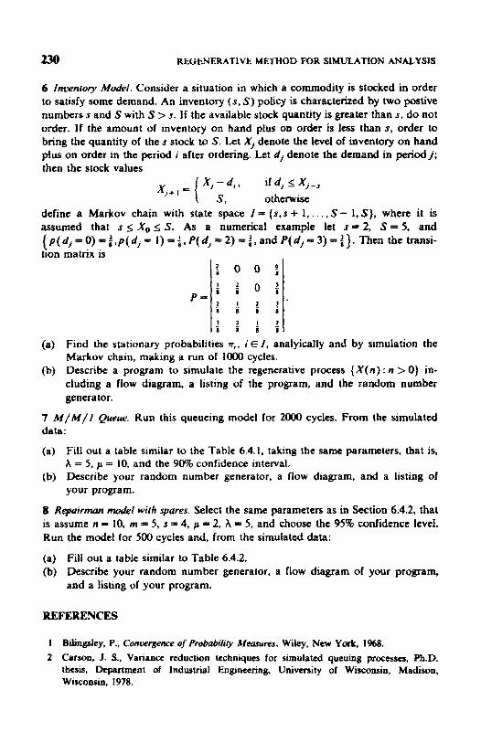
230 REGENERATIVE METHOD FOR SIMULATION ANALYSIS
6 Inventory Model. Consider a situation in which a commodity is stocked in order to satisfy some demand. An inventory (s, S) policy is characterized by two postive numbers s and S with S > s. I f the available stock quantity is greater than s, do not order. If the amount of inventory on hand plus on order is less than s, order to bring the quantity of the s stock to S. Let Xi denote the level of inventory on hand plus on order in the period i after ordering. Let dj denote the demand in periodj; then the stock values
Xj - d i , if dj I Xj-, xi+l= { s, otherwise
define a Markov chain with state space I = (s,s + 1,. . . , S - 1, S}, where it is assumed that s X,, 5 S. As a numerical example let s- 2, S= 5, and { p ( d, = 0 ) = f ,p ( d, = 1) = +, P( d, = 2) = f , and P( d, = 3) = ). Then the transi- tion matrix is
I ? 1 ! ? I 8 1 6 1
(a) Find the stationary probabilities n,, ~ E I , analyically and by simulation the Markov chain, making a run of lo00 cycles.
(b) Describe a program to simulate the regenerative process ( X ( n ) : n > 0 ) in- cluding a flow diagram, a listing of the program, and the random number generator.
7 M / M / I Queue. Run this queueing model for 2000 cycles. From the simulated data :
(a) Fill out a table similar to the Tahlc 6.4.1, taking the Same parameters, that is, X = 5, p = 10, and the 90% confidence interval.
(b) Describe your random number generator, a flow diagram, and a listing of your program.
8 Repuinuur maiel with spares. Select the same parameters as in Section 6.4.2, that is assume n - 10, m = 5, s = 4, p = 2. A = 5, and C~OQSC the 95% confidence level. Run the model for 500 cycles and, from the simulated data:
(a) Fill out a table similar to Table 6.4.2. (b) Describe your random number generator, a flow diagram of your program,
and a listing of your program.
REFERENCES
I Bilingsley, P., Conwrgence of Pro&&& Measures, Wiley, New York, 1968. 2 Carson, J. S., Variance reduction techniques for simulated queuing processes, W.D.
thesis, Department of Industrial Engineering, University of Wisconsin, Madison, Wisconsin, 1978.

REFERENCES 231
3 Carson, J. S. and A. M. Law, Conservation equations and variance reduction in queuing simulations. Technical Report 77-25. Department of Industrial University of Wisconsin, Madison, Wisconsin, 1977.
4 Cox, D. R. and W. L. Smith, Queues, Methuen. London, 1961. 5 &ar, E., Introduction to Slochanic Procuses, Prentice-Hall, Engtcwood Cliffs. New
Jersey, 1975. 6 Crane. M. A. and D. L. Iglehart, Simulating stable stochastic systems, I: General
multi-server queues, J. Assoc. Cow. Mach., 21, 1974, 103- 113. 7 Crsne, M. A. and D. L. Igtehart. Simulating stable stochastic systcma, 11: Markov chains,
8 Crane. M. A. and D. L. Iglehart, Simulating stable stochastic systems, 111: Regenerative prooescrea and discrete-event simulations, @er. Re$., 23, 1975, 33-45.
9 Crane, M. A. and D. L. Iglehart. Simulating stable stochastic systems, IV: Approxima- tion tcchnrqucs, Monoge. Sci., 21, 1975, 1215- t224.
10 Crane, M. A. and A. J. Lemoine, An Inrrochrerion to the Rgenemtiw Method for Sirnulotion Ano&is, Springer-Verlag, New Yo& 1977.
11 Esary, J. D., F. Roschan, and D. W. Walkup. Asgociation of random variables with application, Ann. Mofh. Stoi., 38. 1967, 1 6 1 4 7 4 .
12 Fiacso. A. V. and G. P. McCormick, Nonlinear Progromming: Sequential Uncomtroined Minimization Techniques, Wiley, N e w Yo& 1966.
13 Fishman, G. S., Concepts and Methods in Discrete Digi t4 Sitnularim, Wiley, New York, 1973.
14 Fishman. G. S., Statistical analysis for queueing simulations, Manuge. Sci., 20, 1973,
15 Fishman, G. S., Estimation in multiservcr queueing simulations, W r . Ru., 22, 1974,
16 Fishman, G. S., Achieving specific accuracy in simulation output analysis, Convn. Assoc.
17 Gass, S. I., Linuor Programming Mefiwds and Applications, 3rd ed, MaSraw-Hiil. New York, 1969.
18 Gavcr, D. P. and G. S. Shcdler, Control variable metbods in the simutation d a model of a multiprogrammed computer system, Nm. Re#. Lagist. Qwt . , 18, 1971.435-450.
I9 Gavcr, D. P. and G. L. Ihompson, Progromiftg and Probabiiiq Madels in Operatiom Reseurch, Brooks/Colc, Monterey, California, 1973.
20 Gunther, F. L., The almost regenerative method for stochastic system simulations, Technical Report ORC 75-21, Operations Research Center, University of California, Berkeley, California, 1975. Heidelberger. P., Variance reduction techniques for the simulation of Markov processes, Ph.D. thesis, Department of Operations Research, Stanford University, Stanford, Cali- fornia, 1978.
22 Heidelberger, P. and M. Meketon, Bias reduction in regenerative simulation, Research Rcport RC 8397, IBM Corporation, Yorktown Heights, New York, 1980.
23 Heidelberger. P. and D. t. lglehart Comparing stochastic systcms using regenerative simulation and cnmrnon random numbers, A&. Appl. Prob, 11. 1979, 8w-819.
24 Heidclberger. P.. Variance reduction techniques for the simulation of Markov processes, 1: Multiple atimates, IBM J. RCS. k f q . (to appear).
J. A m . C~nlp. Mach., 21, 1974, I 14- 123.
363- 369.
72- 78.
COW. Mach., 29, 1977,310-315.
21
232 REGENERATIVE METHOD FOR SIMULATION ANALYSIS
25
26
27
28
29
30
31
32
33
34
35
36
37
38 39 40
41
42
43
44
45
Heidclbcrger, P., Variance reduction techniques for the simulation of Markov processes, 11: Matrix iterative melhods, Acfu I n j m . , 13, 1980. 21-37. Heidelbcrgcr, P., A variance reduction technique that increases the regeneration frequency, in Cwrent Issues in Cowpurer Simulation, Academic, New York, 1979, pp.
Hordijk, A.. D. L. Iglehart, and R. Schassbergcr, Discrete time methods for simuiating continuous time Marka, chains, A&. Appl. Prob., 6, 1976,772-788. Iglehart, D. L., Simulating stochastic syslcms, V: Comparison of ratio estimators, Nrm. Rex. k i s t . Qwm., 22, 1975, 553-565. [&hart, D. L., Simulating stable stwhastic systems, VI: Quantile estimation, J. Assoc.
Iglehart, D. L., Simulating stable stochastic systems, VII: Selecting best system, in Aigwirkmic Met& in Probobili@, Vol. 7, edited by M. Neuts, North-Holland, Amster- dam. l977,37-50. Iglchart. D. L, Regenerative simulation for extrcme value+, Technical Report 43, Dqmrtment of Operations Research, Stanford University, Stanford, California, 1977. Iglehart, D. L. and P. A. W. Lewis, Variance reduction for regenerative simulations, I: Intern1 control and stratified sampling for queues, Tochaical Report 86-22, control Analysis Corporation, Palo Alto, California, 1976. Iglehart, D. L. and G. S. Shedler, Regenerative simulation of response times in network of queues, J. Assoc. Comp. Mach.. 25, 1976,449-460. Iglehart, D. L. and G. S. Shedler, S&ulation of response times in finitecapacity open networks of queues, Oper. Ru., 26, 896-914. Iglehart, D. L. and C. S. ShcdIcr, Regenerative simulation d response times in networks of queues, 11: Multiple job types, Rescarch Report RJ 2256, IBM Corporation, San Jose, California, 1978.
Iglebert, D. La, The regenerative metbod for simulation analysis, in Cwrenr Trent& in Pw&rurnnu'w M E I M L ~ , Vsl "1, S%jtw.ar* Ew;newi~, rditd by YL. k& Cknady ond R, T. Ycb, &ntic;c-Hall, Enytewvod Cliffs, New J q , 1978. Iglehurt, D. L. and G. S. Shcdler, Regenerative simulation of response times in networks of queucar, Springer-Verlag, New York, 1980. Iglehart, D. L., Regenerative simulation. Forthcoming. Kubak, I. W., Stopping rules for queueing simulations, Uper. Ru., 16, 1968,431-437. Karlin, S. and H. M. Taylor, A First Cmrse in Stochaslie Pnrccssc~, 2nd ed., Academic, New York, 1975. Kiefer, J. and J. Woifowitz, On the tkory of queues with many servers, Trans. Amer.
Knuth, D. E., f i e Art o/ Computer P r o g m ' n g , Vol. 2, Seminumtieal Algorithms, Addison-Wesley, Reading, Massachusetts, 1969. Lauenberg, S. S., Efficient estimation of work ram in closed queueing networks, in Proceedings in Conpurcuid Stufisiics, Physica Verlag, Vienna, 1974, pp. 353-362. Lavenbcrg, S. S., Regenerative simulation of queueing networks, Research Report RC 7087. IBM Corporation, Yorktown Heights, New Yo&. 1978. Lavenberg, S. S., T. L. MotUer, and C. H. Sauer, Concorninant control variables applied to the regenerative simulation of queueing system, #per. Ru.. 21, 1979, 134- 160.
257-269.
COW. M a h . , 23, 1976,347-360.
Muth. SW., 78. 1955, I- 18.

REFERENCES 233
46
47
48
49
50
51
52
53
54
55
56
57
58
59
60
61
62
63
64
Lavenberg, S. S., T. L. Moeller, and P. D. Welch. Control variables applied to the sirnubation of queueing models of computer systems, in C o m e r Per/omumce. North Holland Amsterdam, 1977. pp. 459-467. Lavenberg, S. S.. T. L. Moelkr. and P. D. Welch, Statistical results on multiple control variables with application to variance reduction in queueing network simulation, Re- search Report RC 7423. 1BM Corporation, 1978. Lavenbcrg, S. S. and C. H. Sauer, Sequential stopping rules for the regenerative method of simulation, 1EM J. Res. k l q . , 21, 1977. 545-558. Lavenberg, S. S. and G. S. Shedler. Derivation of confidence intervals for work rate estimators in a closed queueing network. Soc. lndust. Appi. Math. J . Cw., 4, 1975,
Lavenberg, S. S. and D. R. Slutz, Introduction to regenerative simulation, IEM J. Res.
tavenberg. S. S. and D. R Slutz. Regenerative simulation of an automated tape library, IBM J. Res. Develop., 19, 1975,463-475. Law, A. M., Efficient estimators for simulated queueing system, Technical Report ORC 74-7. Operations Research Center, University of California, Berkeley, California, 1974. Law, A. M., Efficient estimators for simulated queueing systems. Manage. Sci., 22, 1975,
Law, A. M.. Confidence intervals in discrete event simulation: A comparison of replica- tion and batch means. Technical Report 76-13, Department of Industrial Engineering, University of Wisconsin, Madison, Wisconsin, 1976. Law. A. M. and J. S. Carson, A sequential procedure for determining the length of a steady-state simulation, Technical Report 77- 12, Department of Industrial Engineering, University of Wisconsin, Madison. Wisconsin, 1977. Law, A. M. and W. D. Kelton, Confidence intervals for steady-state simulations, 11: A survey of sequential procedures, Technical Report 784, Department of Industrial En- gineering, University of Wisconsin, Madison, Wisconsin, 1978. Lewis, P. A. W., A. S. Goodman, and J. M. Milter, A pseudo-random number generator for the System/360, IBM Syst. J.. 8. 1969, 199-200. Mitchell, B., Variance reduction by antithetic variates in GI/G/I qwuaing simulations, W r . Res., 21. 1973, 988-997. Poliak, D. G., Some methods of efficient simulation for queueing system, Eng, Cybern.
Robinson, D. W., Determinants of run lengths in simulation of stable stochmtic systems, Technical Report 86-21, Control Analysis Corporation, Palo Alto, California, 1976. Rubinstein, Y. R., Selecting the best stable stochastic system, Stochasik Processes Appl.,
Rubinstein. Y. R. and A. Karnovsky, The regenerative method for constrained optimiza- tion problems, in OR’79, edited by K. B. Haley. North-Holland, Araslcrdam. 1979,
Seila, A, F., Quantile estimation methods in discrete event simulations of stochastic systems, Technical Report 76-12, Curriculum in Operations Research and Systems Analysis, University of North Carolina, Chapel Hill. North Carolina, 1976. Varga, R. S., Murrix Iteratiuc Analysis, Prentice-Hall, Englewood Cliffs. New Jersey, 1%2.
108- 124.
D e ~ l o p . , 19. 1975,458-462.
30-41.
(J’SY), I, 1970, 75-85.
10, 1980. 75-851.
931-949.

C H A P T E R 7
Monte Carlo Optimization
Optimization is the science of selecting the best of many possible decisions in a complex real-life environment. The subject of this chapter is Monte Carlo optimization, a subject playing an important role in finding extrema-- that is, minima or maxima of complicated nonconvex real-valued functions. We show how Monte Carlo methods can be successfully applied while solving complex optimization probIems where the convex optimiza- tion methods (see Avriel [Z]) fail. Before proceeding to the rest of the chapter, however, we explain what we mean by local and globd extrema for unconstrained optimization.
Consider a real-valued function g with domain D in R". The function g is said to have a local maximum at point x* f D if there exists a real number S > 0 such that g(x) 2 g(x*) for all x E D satisfying IIx - x*ll c 6. We define a local minimum in a similar way, but in the sense that inequality g ( x ) 5 g(x*) i s reversed. If the inequality g(x) 5 g ( x * ) is re- placed by a strict inequality
g( x ) < g( x * ) , x E D, x it x*,
we have a strict local maximum: and if the sense of the inequality g c x ) < g(x*) is reversed, we have a strict local minimum. We say that the function g has a global (absolure) maximum (strict global maximum) at x* E D if g(x) I g(x*) , f g ( x ) < g(x*)J holds for every x E D. A similar definition holds for a global minimctm (strict global minimum). A global maximum at x* implies that g ( x ) takes on its greatest vahe g(x*) at that point no matter where else we may search in the set D. A local maximum, on the other hand, only guarantees that the value of g ( x ) is a maximum with respect to other points nearby, specifically in a ®ion about x* .
234
Simulation and the Monte Carlo Method R E W E N Y. RUBINSTEIN
Copyright 0 1981 by John Wiley & Sons, Inc.

RANDOM SEARCH ALGORITHMS 235
Thus a function may have many local maxima, each with a different value of g(x), say, g(x;), j - 1, ..., k . The global maximum can always be chosen from among these local maxima by comparing their values and choosing one such that
where
x* E ( x , " , j = 1 ,..., k } ,
I t is clear that every global maximum (minimum) is also a local maximum (minimum); however, the converse of this statement is, in general, not true. If g(.x) is a convex function in R" and D C R" is a convex set then every local minimum of g at x E D also a global minimum of g over D [2].
7.1 RANDOM SEARCH ALGORITHMS
Consider the following deterministic optimization problem:
(7.1.1)
where g( x) is a real-valued bounded function defined on a closed bounded domain D c R". It is assumed that g dchieves its maximum value at a unique point x*. The function g( x ) may have many local maxima in D but only one global maximum.
When g(x) and D have some attractive properties. for instance, g(x ) is a differ- entiable concave function and I1 is a convex region, thcn, as previously mentioned, a local maximum i s also a global maximurn and probleni (7. I . 1) can be solved explicitly by mathematical programming methods (see Avriel [2]). If the problem cannot be solved explicitly, then numerical methods, in particular Monte Carlo methods, can be applied. For better understanding of the subsequent text we describe an iterative gradient algorithm, assuming for simplicity that the set D = R".
According to the gradient algorithm, we approximate the point x* step by step. If on the ith iteration ( i = 1,2,. . . ) we have reached point x,, then the next point x,+, is chosen as
x , + , = x , + a , V g ( x i ) , a , > O (7.1.2)
where
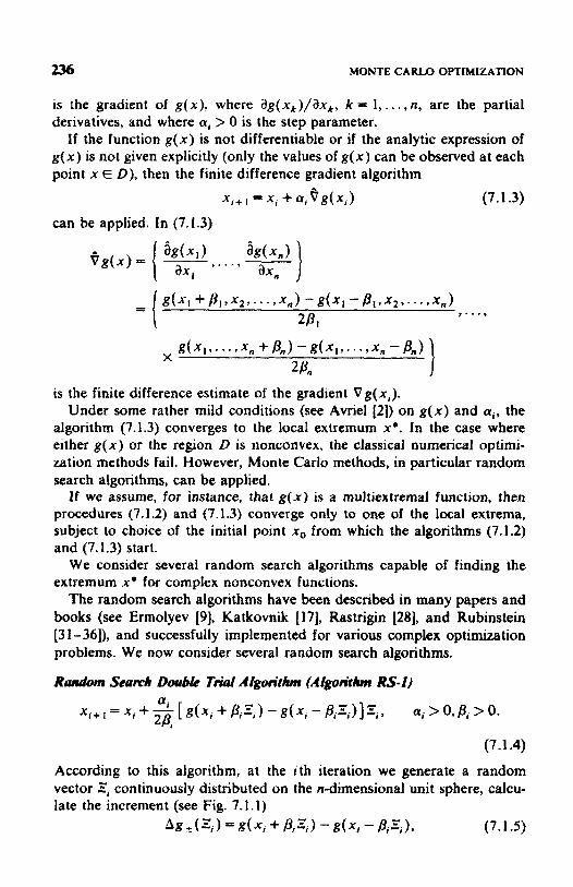
236 MONTE CARLO OPTIMIZATION
is the gradient of g(x), where i 3 g ( x k ) / b k , k = 1,. . . , n, are the partial derivatives, and where a, > 0 is the step parameter.
If the function g(x) is not differentiable or if the analytic expression of g( x) is not given explicitly (only the values of g( x) can be observed at each point x E D), then the finite difference gradient algorithm
x,+ I = x, + a, $g(x,) (7.1.3)
can be applied. In (7.1.3)
is the finite difference estimate of the gradient Vg(x,). Under some rather mild conditions (see Avriel [2]) on g(x) and a,, the
algorithm (7.1.3) converges to the locai extremum x*. In the case where either g ( x ) or the regton D is nonconvex, the classical numerical optimi- zation methods fail. However, Monte Carlo methods, in particular random search algorithms] can be applied.
If we assume, for instance, that g(x ) is a rnultiextrernal function, then procedures (7.1.2) and (7.1.3) converge only to one of the local extrema, subject to choice of the initial point xo from which the algorithms (7.1.2) and (7.1.3) start.
We consider several random search algorithms capable of finding the extremum x* for complex nonconvex functions.
The random search algorithms have been described in many papers and books (see Ermolyev 191, Katkovnik [ 171, Rastrigin [28j, and Rubinstein [3 1-36]). and successfully implemented for various complex optimization problems. We now consider several random search algorithms.
Rpndom Seawh D d k T d Algm'thm (Algorithm RS-I) a,
x,+, = x, + - g(x, + p,Z,) - g ( x , - &Zi) JZ,, a,. > O,P, > 0. 2 4 (7.1.4)
According to this algorithm, at the ith iteration we generate a random vector S, continuously distributed on the n-dimensional unit sphere, calcu- late the increment (see Fig. 7.1.1)
Ag -t ( ', 1 = g t xi + Pi ' 1 ) - g( x j - f i n Ej 1 1 (7.1.5)
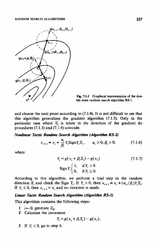
RANDOM SEARCH ALGORITHMS 237
Fii. 7.1.1 Graphical repnsentation of the ble trials random search algorithm RS-1.
dou-
and choose the next point according to (7.1.4). It is not difficult to see that this algorithm generalizes the gradient algorithm (7.1.3). Only in the particular case where Zl is taken in the direction of the gradient do procedures (7.1.3) and (7.1.4) coincide.
Nunlinear Tacric Rmulom Smwh Algodhm (AlgO&hm RS-2) x t + , = x , + -YiSignY,Ei, a; a,>O,j3,>0,
Pi (7.1.6)
(7.1.7)
I , U x > O 0, ify L O .
Sign U,
According to this algorithm, we perform a trial step in the random direction E, and check the Sign Y,. If > 0, then x,, , = x , + (a , /PI)YE, . If U, I 0, then x , , , = x, and nu iteration is made.
Linear Tactic Rondom Sea& Algorithm (Algoriflun RS-3) This algorithm contains the following steps:
1 i t 0 , generate &. 2 Calculate the increment
Y, =g(xi + PtZ,) -gfxi).
3 If Y, < 0, go to step 6.

238 MONTE CARL0 OPTIMIZATION
4 a
x,, , = xi + 2 YEi, ai > 0, pi > 0. PI
(7.1.8)
5 Go to step 7. 6 x i f l tx i . i t i + 1; generate zl. 7 Go to step 2.
Thus if 5 > 0, we perform as many iterations as possible in the initial chosen random direction xi + /3,Ej- ,; if y. 5 0, we generate a random vector Sj and perform only one iteration according to the nonlinear tactic random search algorithm RS-2.
It is not difficult to see that search in the same direction versus choice of a new direction is subject to the shape of g(x ) . The flatter the gradient lines, the more iterations will be performed according to step 4 and correspondingly the fewer iterations according to step 6. In the particular case where g ( x ) is a linear function, all iterations will be performed according to step 4 in the direction of the vector xo + a + ao&- 'YoE0, where Z, is the first random vector such that Y , > O and no iteration will be performed according to step 6. This is the reason why this algorithm is called a linear tactic random search algorithm.
Optimum Trial Random Search Algori th (Algoritrhm RS-4)
This algorithm comprises the following steps: Choose N > 1 independent random points xi + /?& on the sphere
{xi + PIEi}, where Zi is a random vector continuously distributed on the unit sphere with reahations k = 1,. . . .IV.
-
1
2 Consider the sequence of increments
and let Z,$ denote the direction that has produced this maximum. 4 ' fie p i n t x,+, is chosen according to the following iterative proce-
dure:
x i + , = x, + a , f i i - l ~ ~ , Z ~ ' , ai > O, pi > 0. (7.1 . I 1)
Thus the next point x , + ~ is chosen in the direction E,$ of the greatest increase x g of the function g(x), that is, the vector Z$, corresponds to the trial optimal among those available.
RANDOM SEARCH ALGORITHh4S 239
Stahtimi Gmdient Rrrndom Search Algorithm (Algorithm RS-5) This algorithm can be described as follows.
( x i + bizi}, where unit sphere with realizations Z i k , k = 1 ? . . . , N .
1 Choose N > I independent random points xi + bizjk on the sphere is a random vector continuously distributed on the
2 Calculate the sequence of increments
Kk =g(xi + pisik) - g ( x i ) , 3 Set
k = 1, . . . , N . (7.1.12)
(7.1.13) 1 ” &=- 2 VkSik .
k-i 4 The point x i + , is chosen according to
x i + l 5 xi + aiPi-lV,.s, a; > 0, Pi > 0. (7. I . 14)
Thus given x i , the next point xi+ I is chosen in the direction which is a result of averaging the sample Zil, . . . ZiiN weighted with their correspond- ing increments xk (7.i.12). In the particular case where N = n and - + = e k , = O ...., 0 . 1 , O , . . , , 0, k = I ,..., n, -
k
we obtain the foltowing finite difference gradient algorithm:
where Xi+L = x, + a , b ( x , ) (7.1.1 5 )
) - g(x, -4- @ I , % * , . . . , x n ) - g(-r) gtx,, . . . ‘X, + f i n ) - g ( x ) . . . . I
1 3 1 P n
It is not difficult to prove that for a linear function the direction of qe, on the average, coincides with that of the gradient of g(x). This is the reason why the algorithm is called “statistical gradient algorithm.’’
Consider the following srochasfic opfimization problem.
max “ E [ + ( x , W ) ] = max g ( % ) = g ( x * ) = g * . (7.1.16) x E D c R x E D c R ”
Here + ( x , W ) is a function of two variables, x and W, x* is the optimal point of g(x), which is assumed to be unique, and W is an r.v. with unknown p.d.f. fw(w). We assume that at each point x E D only the individual realization of +( x, W ) can be observed.
It is clear that, if the p.d.f. j w ( w ) is unknown, probiem (7.1.16) cannot be solved analytically. However, numerical methods can be applied.

240 MONTE CARLO OPTIMlWTION
One widely used numerical method for solving (7.1.16) is the srochastic approximation method. This method was originated by Robbins and Monro [30], who suggested a procedure for finding a root of a regression function measured with a noise. Kiefer and Wolfowitz [ 191 considered a procedure for finding x* in the optimization problem (7.i.16) where x E R'. The procedures of Robbins-Monro and Kiefer-Wotfowitz were generalized by Dvoretzky 181. Hundreds of papers and many books have been written in the past I5 years about stochastic approximation, their convergence, and their applications. The reader is referred to Wilde [44] and Wasan [43].
We consider the following algorithm:
x , + I = x , + a , ~ + ( x , ~ K), (7.1.17)
where
+(x, + B L , X * , . . , x n , Wl,) -@(x i - P I , X Z , . . * ?X,, W,2) 28,
$4x,, x 2 , . . . * x, + P, , W,,) - 44x1 7 x2 1 . . * 7 x, - Pn, Wn2)
28,
,...,
1 is the estimate of the gradient fig(x).
It is readil seen that in the absence of noise, that is, when W - 0 , 6+(x, W ) =Jg(x) and (7.1.17) coincides with (7.1.3). In addition, if the realizations of the noise ar,e independent and E( W) = 0, then 6+(x, W ) is an unbiased estimator of V g ( x ) .
Proof of convergence of algorithm (7.1.17) to x*, subject to some conditions on the sequences (al)zr, and the function +(x, W), can be found, for instance, in Dvoretzky (81, Gladyshev [13j, and Wasan [43].
I t is not difficult to understand that the random search algorithm can also be used for solving problem (7.1.16). For instance, by analogy with (7.1.17) the random search double trial algorithm (Algorithm RS-I) can be written as
a X , + ~ = X , +--"[+(x,+ P I E , . q,) - + ( x i F2) ]E , . (7.i.i8)
We can see that, for the same reasons as the random search algorithm (7.1.4) extends the gradient algorithm (7.1.3), the random search algorithm (7.1.18) extends the stochastic approximation algorithm (7.1.17).
Proof of convergence of (7.1.18) to x* can be found in Rubinstein [31). In analogy with (7.1.18) we can adopt any of the random search algorithms RS-2 through RS-5 for solving problem (7.1.16).
2/31

EFFICIENCY OF THE RANDOM SEARCH ALGORITHMS 291
7.2 EFFICIENCY OF THE RANDOM SEARCH ALGORIT)?MS
The random search algorithms can be compared according to different criteria. Usually, they are compared according to their local and integral properties [28, 291.
Local properties are associated with a single iteration of the random search algorithm, integral properties-with many iterations. Comparing dif- ferent algorithms according to integral properties we usually define:
I The initial condition from which search starts. 2 A set of test functions (linear, quadratic, parabolic, multiextremal,
etc.) for which the extremum is sought. 3 Some criteria that must be achieved during optimization. The follow-
ing criteria can be used. Find an index k corresponding to the best algorithm among S algorithms available, such that:
(a)
where the number of iteration i is given. t w

242 MONTE CARLO OPTIMIZA'IION
I t is readily seen that the first three problems are associated with finding the best algorithm when the number of iteration i is given; the last two involve finding the best algorithm that hits, at the minimum number of iterations, a given region R, or R , containing the extremum point x*. In Section 7.3 we consider some local and integral properties of Algorithm RS-4.
Generally, the problem of comparison of different algorithms according to their integral properties is difficult to solve. Some attempts to overcome this difficulty have been made by Rastrigin [28]. Another interesting problem is how to find the optimal combination of algorithms, each of which is capable of finding the extremum of g(x). This problem is solved in Rubinstein [33] and uses Bellman's principle of optimality.
Now we consider some local properties of the random search algorithms, assuming that some point x, has been reached, and that we are allowed to make only a single step (iteration). Let x!:)~, s = I , . . . , S, be the point (the state of the system) after this single iteration. Let us define the efficiency of the random search algorithms as
(7.2.1)
where
that is, where Axfa) is the projection of the vector x!:), - x, on the direction of the vector x, - x*. and 4(*' is the number of observations (measure- ments) of g(x) required for the algorithms in the ith step. For simplicity we consider only the case where g ( x ) is approximately a linear function, which is the same as to assume that in Taylor expansion
g ( ~ , + , ) = ~ ( ~ , + ~ X , ) ~ ~ ( ~ , ) + ~ ~ ~ , ~ V ~ ( ~ , ~ ~ + ~ ( ~ ~ , ) . (7.2.2) Therefore at each iteration made by the random search algorithms, we approximate gfx) IinearIy on the interval Ax,. It is proven in (32) that, for a rather wide class of functions optimized by random search algorithms under the conditions
m OD
I - I i - I
there exists a number I, sufficiently large and such that for i 1 1 a linear approximation of g(x), that is, (7.2.2), is valid.
Substituting (7.2.2) in any of the four random search Algorithms RS-1, RS-2, RS-4, and RS5 (see, respectively, (7.1.4). (7.1.6), (7.1.11), and

EFFICIENCY OF THE RANDOM SEARCH ALGORITHMS
(7.1.14)), we readily obtain
243
, v ~ ~ ~ , = x, + a ~ ’ ) V g ( . x , ) cos p!*’ i- o( AX^"') (7.2.3)
where
and s = I , 2,4,5 corresponds to RS- I , RS-2, RS-4,
(7.2.4)
and RS-5. The distribu- tion of ‘p!’) depends on the specific algorithm and on the distribution of the random vector E!:,’”). Let us assume without loss of generality that afs)= 1. Then taking into account that for a linear function g(x) the direction of the vector x* - xi coincides with the direction of the gradient V g ( x i ) , we can express the efficiency C, (see (7.2.1)) as
E(c0s py) c, = E( A!(”)
(7.2.5)
We consider here only the efficiencies of the random search Algorithms RS-I, and RS-4, assuming that the vector E is uniformly distributed on the surface of the unit n-dimensional sphere.
(a) The Double Trial Random Search Algorithm RS-1 (7.1.4). (7.2.3). and (7.2.4) that
It follows from
where p!’) is a random angle between t b vector 2:’) uniformly distributed on the n-dimensional sphere and the vector V g ( x , ) . We assume here that the direction of the gradient corresponds to ‘p;”=O. Furthermore, it follows from (7.2.5) that the distribution of d’) does not depend on i ; therefore the index i can be omitted. We also omit for convenience index (1) in d’). I t is shown in the Appendix that pl has a p.d.f.*
(7.2.6) 7r 7r
h,(cp) = B,sinn-2cp, - - < ‘p 5- 2 - 2 ’
where
(7.2.7)
*We use for convenience - 5 rp I 7 rather than 0 5 p 5 n (see Appendix).

244 MONTE CARLO OPTIMIZATION
Since for Algorithm RS-I we need two observations of g(x) at points g(x + B E ) and g(x - BE), respectively, the efficiency C, (see (7.2.5)) is
C,”’= E(coscp) 2 .
The expected value and the variance of cos cp are, respectively,
(7.2.8)
(7.2.9)
(7.2.10)
Substituting (7.2.9) in (7.2.81, we obtain
B n c, = - n - 1
and the following relationships can also be easily
(7.2.1 1)
verified :
Table 7.2.1 and Fig. 7.2.1 represent the efficiency C,, and var(cos p) = u2 as
Table 7.2.1 The Efficiency and u’ ss FurrdiolrP d II for Aigod?bm RS-1
0 2
2 3 4 5 6 7 8 9
10 I 1
0.3 184 0.25 0.2125 0. I875 0. I702 0.1556 0.1452 0.1367 0.1294 0.123
0.5995 0.416 0.314 0.26 0.22 I 0.1957 0.166 0.1401 0.1344 0.2268
0.41 12 0.3876 0.3792 0.3677 0.3602 0.3518 0.3564 0.3652 0.3529 0.3538
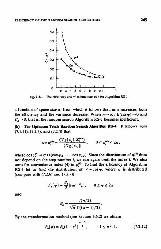
EFFICIENCY OF THE RANDOM SEARCH ALGORITHMS 245
; 0.3
0.2 ;_I 0. I
\ 9
0 2 3 4 5 6 7 8 91011
Fig. 7.2.1 'f ie efficiency and y2 as functions of n for Algorithm RS-I.
a function of space size n, from which it follows that, as n increases, both the efficiency and the variance decrease. When n+oo, E(coscp)-+O and Cn-+O, that is, the random search Algorithm RS-I becomes inefficient.
(b} The Optimum Trials Random Search Algorithm RS4 It follows from (7.1.1 I), (7.2.3), and (7.2.4) that
where cos qy) = max(cos vir, . . . , cos pi#). Since the distribution of v:*) does not depend on the step number i, we can again omit the index i. We also omit for convenience index (4) in 91:'). To find the efficiency of Algorithm RS-4 let us find the distribution of Y==eoscp, where cp is distributed (compare with (7.2.6) and (7.2.7))
and
By the transformation method (see Section 3.5.2) we obtain n - 3 -
P,(o)= Bn(l 4) * , - 1 5 0 5 1 . (7.2.12)

246 MONTE CARLO OPTIMIZATION
The c.d.f. and p.d.f. of V: = max( V, , . . . , V, ) are, respectively,
F , ( 4 ) = [ F,(41N (7.2.13)
and
P , ( ” ; } = ” F , ( o ) ] ” - ’ P,(u). (7.2.14)
The expected value and the variance of Vi are, respectively,
(7.2.15)
For n = 3 we have
P3(uoN)=$l N + t ) ) N - ’ (7.2.17)
N - I N + l E( v$) = - (7.2.18)
(7.2.19) 4N var( v,,} =
( N - 1)“ + I t follows from (7.2.5) that the efficiency of Algorithm RS-4 is
For n = 3 we obtain ( N - I )
c 3 = ( N + 1)”
(7.2.20)
(7.2.2 1)
The optimal value of C, equals i and is achieved when N is equal to 2 or 3. Generally, it is difficult to find C, and var(V,O) for n > 3. Table 7.2.2 and
Fig. 7.2.2 represent simulation results for C, and var( V,”) as a function of n for the optimal number of trials N+ on the base of 100 runs. It is interesting to note that the optimal N* = 2 and does not depend on n.
Comparing Algorithms RS-1 and RS-4 for a linear function, we con- clude that RS-I is more efficient than RS-4 for all n > 1. The variance associated with Algorithm RS-4 for the optimal N* = 2 is always less than that associated with RS-1. The intuitive explanation for it can be given as follows. Taking two random trials according to Algorithm RS- I, we always

EFFICIENCY OF THE RANDOM SEARCfl .ALGORITHMS 241
Table 7.2.2 Tbe Efficiency and the var( V , ) as Functions of II for Algorithm RS-4
cn n Cn varf v:) N* -
3 0.198 0.236 2 4075 4 0.159 0.171 2 3845 5 0.137 0. I34 2 3743 6 0.121 0.1 10 2 3647 7 0.109 0.053 2 3575 9 0.092 0.070 2 3478
11 0.08 I 0.050 2 3622
0
Note: The sample size is equal to 100.
find a feasible random direction toward the extremum, which is generally not true for Algorithm RS-4. Indeed, the probability of finding such a direction (success) in N independent trials is equal P ( N ) = I - ( I -p)” Here p is the probability of success in a single trial. Taking into account that for a linear function p = l , we obtain, for the optimal N+ = 2. P( N* = 2) = a , that is, the probability of a success in Algorithm RS4 is equal to f - Defining khe efficiency as CdS)/u(’)), where o(’)= (var(cosrp(’))J’/*. we see from Tables 7.2.1 and 7.2.2 that both Algorithms RS-I and RS-4 have approximately the same efficiency.
\
0 . 2 5 0.20 t 0.05 1
0 2 3 4 5 6 7 8 9 1011 n
Fig. 7.2.2 The efficiency and the var(V:.) as functions of n for Algorithm S-4 (the sample size is equal to 100).

248 MONTE CARLO OPTIMIZATION
73 LOCAL AND INTEGRAL PROPERTIES OF THE OPTIMUM TRIAL RANDOM SEARCH ALGORITHM RS-4
This section is based on Ref. 35.
73.1 Local Properties of the Algorithm
The term "local properties" refers here to convergence of the vector x,+ , - x, to the direction of greatest increase of the function g(x) , as the number of trials m tends to infinity.
Assume that g(x) is a continuous function and
+(x, W ) = g ( x ) + W , x E D c R", (7.3.1)
that is, each measurement of the function g(x) is accompanied by additive noise W, and assume that the vector Z is continuously distributed on the unit sphere with a densityf(Z). Let B be the set on the surface of the unit sphere defined by the condition f (Z) > 0 and let B be the closure of E . Let us also assume that the maximum
(7.3.2) maxg(x + BZ) -g( x + PZ')), 2' E ii IEB
occurs a1 the unique point x + pro.
optimum-trial directions ( E ~ > ~ - , defined by We are concerned with the asymptotic behavior of the sequence of
Theorem 73.1 Vector Ev is almost surely (as.) the only limiting vector of the sequence {E2)zE, if and only if the noise W satisfies the following property: For a s . any sequence ( W,}:-, of W's realizations and for any c > 0, there exists a natural number K , (which depends on the sequence) such that
W,< Fk+c, K , I k < c n , (7.3.4)
where - W, = max W,.
I < l < k - l (7.3.5)
Proof (1) Suffiency Let us prove that for every 6 >0, the 6- neighborhood S( Eo, 8 ) of the point Zo contains almost all optimum-trial directions E:, when m is sufficiently large. The proof is by contradiction. Assume that there exists 6 > 0 such that the following holds: There is a

LOCAL AND INIEGRAL PROPERTIES OF TIIF. RANDOM SEARCH ALGORITHM 249
positive probability that a realization (Ern): contains a subsequence (Z,,,}r- such that
g ( x + p E m , ) + Wmh>g(x+@Z,)+ y , 1 S j < m , - 1 (7.3.6)
and at the same time Zrnk B S( so, 6).
Continuity of g(x) implies that we can choose 7 > 0 and 6, < 6, such that inf g(x + P Z ) > sup g(x + p S ) + 27. (7.3.7)
E Bn s( E", 8 , )
The case of unbounded noise Assume the sequence { Wmk)y- is
Wm4< wmk+ 0 , mk > K, (7.3.8)
Denote by Zk the number of the trial in which the maximum qmk is achieved, that is, WS4 = Kmk and iiik < mk hold. The sequence of indices (Eik)';9ct is a.s. unbounded, because { Wml)T=, is as . unbounded. Therefore &he event
E- "ko E Bln S( z0, 6,) will as. occur for some Eke> K,, since at each trial there is a constant nonzero probability of its occurrence. Comparing the results obtained in trials iEk, and mko, it follows from (7.3.7) and (7.3.8) that
3 E if/( I@. 6)
(a) unbounded and satisfies
B( x + P',iiko) + w,ii.,> g(" + B'rnb0) + Wmro+ 7 s
which contradicts (7.3.6). Q.E.D. If sup W = Wmx < m, then the
sequence { Wrn>z, , as. contains an infinite subsequence { W , , ) ~ , such that
On the other hand, there exists as. a particular subscript miO such that
(b) The case of bounded noise.
W,,,,,-q< Wm,5 Wmx, i = 1,2, ...
z 4 0 E Bn S(Z*,&,). Thus fcr any m > mio satisfying Em B S(?, S),
g ( x + P m , , , ) + Wm,*> gtx + @Ern) + Wm, + 7)
g(x + gzm) + Wm, which contradicts (7.3.6). Q.E.D.
(2) Necessity Assume that the set ?of sequences {Wk}:-t not satisfy- ing the theorem's condition has a probability P ( c ) > 0 For each sequence

250 MONTE CARLO OPTIMIZATION
from c there exists a number c > 0 and a subsequence { Wk,}lm,, such that
wk, 2 Ek, + c. (7.3.9)
Our task now is to prove that with probability P ( c ) the vector Zo is the only limiting vector of the sequence { E:}:- ,. What we actually prove is a somewhat stronger statement: namely, that the set of limiting vectors contains the set
V, = iin { Zlg(x + PS") - c < g(x + pz) I g(x + pro>}. (7.3.10)
To prove this statement it suffices to show that for any y €3 and any S > 0 the sequence {E;}E-, will visit the neighborhood S(y,S) infinitely often. Indeed, for any trial there exists a constant positive probability of entering the set S ( y , 8 ) n V,. This implies that the subsequence of trials (k,} satisfying (7.3.9) as. contains a new subsequence {k,,) such that
E S ( y , 6) n V, holds. The vectors z k , , will be optimum-trial directions, -k,, since for any i , 1 I i 5 k,l- 1,
8(AX + @5k,l ) + wk,l > 8( x + pz' 1 f wk,, =.g(n+pz, )+ w;.
Q.E.D.
Remark In the case without noise ( W = 0 a.s.) we can explicitly calculate the number of trials required to enter a prescribed &neighborhood S( Eo, 6) of the point I' with a prescribed probability p.
Define
that is a is the probability of visiting S(Zo,S) at each single trial. The probability of visiting S(Zo, 6 ) at least once by making rn trials is equal to
p ,= I - ( l - a ) m . (7.3.1 1)
Thus if we want p, 2 p , i t suffices to produce
trials. In the case where p = 1 - a,
In a In(I - a) m 2
(7.3.1 2)
(7.3.13)
Table 7.3.1 shows some values of m as a function of a.
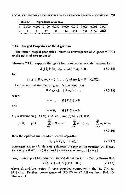
LOCAL AND IN’I‘EGRAI. PROPERTIES OF THE RANDOM SEARCH ALGORITHM 251
TaMe 73.1 Dependence of m 00 a
a 0.500 0.200 0.100 0.050 0.020 0.010 0.005 0.002 0.001
r n l 8 22 58 194 458 1057 3104 6903
73.2 Integral Properties of the Algorithm
The term “integral properties” refers to convergence of Algorithm RS-4 to the point of extremum x*.
Tbeorem 73.2 Suppose that g ( x ) has bounded second derivatives. Let
E( 115, II*Ix(J,xI, . . - 7 x , ) I hf < 00 (7.3.14)
for 11 x, 11 I 5 < 00, j = 0, 1 , . . . , I , where 5, = @,- ’ E$.
Let the normalizing factor y, satisfy the condition
0 < v,( TI II X I I I + A, ) < WJ 9 (7.3.15)
where 7, = 1 ,
7, =r 0,
If l l ~ & l l > o
if II VP, iI = 0
and
( V , is defined in (7.3.18)), and let a, and /3, be such that m m @
a, 2 0, /3, 2 0, I] alp, < 00, 2 /j? < m, 2 a , = 00: 1 - 1 1- I 1 - 1
(7.3.1 6)
then the optimal trial random search algorithm
x, + I = 4 .x, - a,v,E, ) (7.3.17)
converges as . to x * . Here a(.) denotes the projection operator on D (i.e., for every x E R“, n ( x ) E D and IIx - n(x)ll- min,,,llx - Y 11.
Proof Since g ( x ) has bounded second derivatives, it is readily shown that E(Eitxi) = C i V g ( x j ) +P,V,s (7.3.18)
where C, and the vector V , have bounded components, that is, Ci < 00,
IIV,ll < 00. Further, convergence of (7.3.17) to x* follows from Ref. 10, Theorem 1.

252 MONTE CARLO OPTIMIZATION
7.4 MONTE CARLO METHOD FOR GLOBAL OPTiMIZATlON
(a) Deterministic Optimization Problem The problem of finding the global extremum of g( x ) (see (7. I . 1)) has been approached in a number of different ways. The earliest methods were associated with the grid tech- nique and the function was evaluated at equispaced points throughout D. We shall consider only Evtushenko's algorithm [ 1 I ] in such a deterministic sense. Some other deterministic approaches for global optimization are given in Dixon [7], Shubert 1371, and Strongin [39]. Evtushenko makes the foilowing assumptions about the function and the objective:
1 The function satisfies the Lipscitz condition, that is,
Ig(X,)-g(x,)j<~llx,-x,If,
for any xi . x 2 E D, L > 0. 2 Each x E D,, where
0,s { x : tg(x) -g(x*)J < E } ,
is accepted as an approximation for x * .
Evtushenko's algorithm IS as follows.
Algorithm GI- I 1 Evaluate the funclion a1 N equispaced points x,, . . . ,xNthroughout D
and define y, =g(x,), k = 1 , . . ., N.
2 Estimate g* by
The theoretical background to this approach is very simple. Let V , be the
MN = max( y , . . . . ,y, ).
sphere 11 x - x, [I 5 r, where
Then for any x E V,
Hence if the sphere V,, i = I , . ..,N, covers the whole set D, then MN cannot differ from g+ by more than E. and the problem is solved.
In the simplest case where D is an interval, a I x I b, Evtushenko proposed the following procedure:
rt = L . - ' ( g ( . ~ , ) - MN + E ) .
g( x ) 2 g( x,) - Ix, = MN - c,
E x , = u + - M , = g ( x , )
2 E + B ( X & ) - 4 L '
L X&+, = XK + M , = max(g(x,),M,-,).

MONTE CARLO METHOR FOR GLOBAL OPTIMIZATION 253
The number of function evaluations required to solve the problem is greatest in the case of a monotonically increasing function, namely
L ( b - a ) N = 2 E .
Most algorithms for global optimization contain random elements and are related to the Monte Cario method. We consider some such algorithms. Brooks (4) suggested, for solving problem (7.1.1), the following “pure”
random search algorithm.
Aig~dhttt GI-2 1 Generate X , , . . . , X, from any p.d.f.f,(x) such thatf,(x) > 0, when
X E D. 2 Find Y k = = g ( X k ) . k = I ,..., N. 3 Estimateg* by
M, = max( Y,, . . . , YN).
that reference, and our discussion is based on it.
that ( D , B , P ) is a probability space.
This algorithm was also discussed in Ref. 36. Our nomenclature follows
Let p be the probability measure defined on B, the Bore1 o-field of D, so
L e t g - ’ ( a , b ) = { x E D : a < g ( x ) _ < b } , and Iet F ( y ) = P ( Y ; l y ) ; then
F ( y ) = p{ 4 X,) 5 v } = P ( g - ’( - -7Y 1) and Y,, . . . , Y, are independent identically distributed (i.i.d.) random vari- ables (r.v.’s) on R’ with a cumulative probability distribution function (c.d.f.) F.
Proposition 7.4.1 borhood of x+, and suppose g is continuous at s*, then
Suppose P assigns u positive probability to every neigh-
lim MN =g* a s . N + W
(7.4.1)
Proof It is clear that F(g*) = 1 and for each 6 > 0 we have 1 - F(g* - 6) = P ( g * - 6 < g( X , ) 5 g*} > 0 by our assumption. Let A N ( 6 ) be the event (MN 5 g* - 6); then P(A,(6)) = FN(g* - 6) and X g , , P { A , ( 6 ) } = F(g* - 6)/(1 - F(g* - 6)) < 00. By the Borel-Cantelli lemma P { M , ,< g* - 6 infinitely often) = 0 for all d > 0 and thus (7.4.1) follows. Q.E.D.
The choice of P, and consequently the resulting F, depends on our prior knowledge of x’. If it is known that a certain region is more likefy to include x*, then it would be more efficient to assign a higher probability to

254 MONI'E CARLO OPTIMIZATION
that region. If nothing is known a priori about x*, a uniform distribution over D can be assumed.
In guaranteeing (7.4.1) the exact choice of P is immaterial. However, the rate of convergence is determined by the properties of F. For example, by a theorem of Gnedenko [MI, if there exists a constant a > 0 such that
1 - F(g* - 0 5 ) 1 - F(g* - 6 )
lim = c u , v c > o 610
(7.4.2)
then
with aN determined by F(g* - aN) = ( N - l)/N. Some more properties of MN are listed below.
Geometric distribution Let jv8 be the first N for which MN > g* - 6. Then N8 is a geometric r.v., that is,
I
P { N , p k ] =: Fk- ' (g * - 6)[ 1 - F(g* -a) ] . k f ,2, . . . . (7.4.4)
Consequently, it is well known that
- I EN, = = ??& I - F ( g * - 6)
and P ( N 8 5 k } 5 1 -- Fk(g* - 6) ZE P&,t.
I t is clear that ~ ~ 3 0 9 as 640 and thus f6,,,,,l = 1 - ( 1 - l /98)[v~1+l - e - ' = 0.63 (here [q] is the integer part of v). Hence 9)8 = EN, is approxi- mately a 63% confidence bound for N8, the number of trials necessary to make MN > g* - 6 (6 > 0 small). Let a = 1 - F(g+ - 6); then fa$k = 1 - (1 - a)&. For every given pair (a,P) the smallest k for which P8.k 2 P is k( a, 8) = In( 1 - &/In( 1 - a), and Table 7.3.1 with k( a, 1 - a) = nr can be used again.
2 tack of memory I t is well known that (7.4.4) implies P { N b > k + m/Na > m ) = P(Ng > k).
P ( M , + , I g* - SIM, 5 g* - S} = P ( M , I g* - 6 ) ,
(7.4 S)
In terms of N,,, we thus have
because the events {A'& > k} and {Mk 5 g* - 6 ) are identical. It follows that, given m successive failures (to enter ( y : y > g* - 6 ) ) , the conditional distribution of the number of trials necessary for the first success equals its

MONTE CARLO MEI'HOD FOR GLOBAL OPTIMIZATION 255
unconditional distribution. In particular we have E( N, I M, 5 g * - 6 1 = m + EN8. (7.4.6)
3 Poisson approximation If (7.4.2) or (7.4.3) hold, then Z8,,v, the number of q, i = 1.2,. . . , N, for which > g* - 6, is asymptotically Poisson distributed. More precisely, for fixed N and 6 > 0, Z8, , is a binomial r.v. with parameters N and p = I - F(g+ - 8 ) . When (7.4.2) holds by substituting 6 = a N in (7.4.2), we obtain N [ I - F(g* - 6a,)]+c", which implies that Zco, ,N converges in distribution to a Poisson r.v. with parame- ter c".
The problem of finding the global maximum of g ( x ) can be reduced to that of finding the mode for association with g(x) density function. Indeed, if g(x) 2 0, x E D , then $(x) =c-'g(x) where c - ' = ( j g ( x ) d x ) - ' is a density function. and the problems of finding the global maximum of g ( x ) and finding the mode of #(x) are equivalent. This can be solved by one of the methods mentioned in Refs. 41, 42, and 46.
If g(x) is unrestricted in sign but bounded, that is, if Ig(x)l 5 k , then f x ( x ) - c - ' ( g ( x ) + k ) , where c . ' = [ J ( g ( x ) + k ) d x ) - ' is again a density function.
A natural extension of the "pure" random search algorithm GI-2 is the so-called muitistart algorithm [7], which is probably the one most fre- quently used in practice for global optimization. In this approach we use any iterative procedure (gradient, random search, etc.) for local optimi- zation and run i t from a number of different starting points xoJ, j - I , .... N. The set of all terminating points hopefully includes the global maximum x * .
The muitistart algorithm is as follows. Algorithm GI-3
1 Generate Xol , . . . , X,, from any p.d.f.f,Jx-) > 0, x E D (usually X, is chosen to be uniformly distributed over D ) .
2 Consider XoI.. . . , X, , as the starting points, then apply N times a local optimization algorithm (gradient, random search, etc.) and find the local extrema x:, , . . .xfN of g(x) associated with Xol,. . . , XoN.
3. Estimate x * by max (1:. . . . , x:}.
Let us define D, as the set of starting points A', from which the algorithm will converge toj-th local maximum. We call DJ the region ofarrruction of the j th local maximum. Let us assume that the number of local maxima is finite, and let X, be uniformly distributed over D; then the probability

256 MONTE CARLO OPTIMIZATION
of at least one X,, from a sequence of N points drawn at random over D, falling in the region of attraction of the global maximum 0;. equals
(7.4.7)
where m( 0 ) is the measure of D.
A more sophisticated approach to the global optimization problem was suggested by Chichinadze [5], who introduced a probability function P( u ) as the probability of g(x) < c, that is, if m ( V ) is the measure of the level set
Y = { x : g ( x ) < u ) .
then
(7.4.8)
The function P(o) is, of course, not available, but if we calculate g(x) at N points distributed at random over D, and count the number M of these points for which g ( x ) < u, then M / N approximates P( u). It is not difficult to see that the global maximum corresponds to P ( c ) = I and the global minimum to f ( u ) = 0. To find the solution P ( c ) = 1, Chichnadze sug- gested approximating f ( v ) by a linear combination of a set of given polynomial functions P,(u), i = I . . . . , k ,
k P(,) = 2 h,P,( t ; ) . (7.4.9)
r = l
The range of u was divided at the points u,, j = 1, . . . ,s. and the optimal values of A, were determined by minimizing
(7.4.10)
where M, is the number of points for which g ( x ) <u,, and q . > O , j = 1,. . . , s. The root t‘* of P( u) = 1 was then determined to obtain an estimate of the global maximum of g(x).
Considerable attention has been paid in the multiextremal optimization to the random search algorithms. Gaviano [ 121 showed that if
(7.4.1 1) - x,+ I = x, + a,&,
a, = arg ( global max g( x, + arSr)) ,
and (7.4.12)

MONTE CARLO METHOD FOR GLORA!.. OPTIMIZATION 257
then lim P ( g ( x , ) - g( x+) < E ) = I (7.4.13)
for every p > 0. Here E is a vector uniformly distributed on the surface of a unit n-dimensional sphere.
If D is a finite space and if a bound on the first derivative of g ( x ) is known, then Evtushenko's [ 1 11 or Shubert's [371 one-dimensional global optimization techniques could be used to find the optimal ai. However, for a general function, a global optimization along the lines of (7.4.12) is difficult to perform.
Matyas [22] proved the convergence to x' of the foHowing random search algorithm.
Aigorihm GI-4
with zero mean and covariance matrix 2, that is Y - N(0, Z).
i+ 00
1 Generate Y,, Yz, . . . , from an n-dimensional normal distribution
2 Select an initial point xi E D. 3 Compute g(xl). 4 i c l . 5 If x, + Yi ED, go to step 8. 6 x i + - x , + , . 7 Go to step 10. 8 Compute g(x, + Y,). 9
x i + U,, if g( xi + q.) 2 g( xi) - e, where E > 0 i x i 3 otherwise. xi+)-
10 i c i + 1. 11 Go to step 5 .
According to this algorithm, a step is made from the point xi in the direction only if x i + Y, E D and g ( x i + Y,) 2 g ( x i ) - e.
The following procedure, based on cluster analysis, was introduced into global optimization by Becker and Lago [3].
AIgoritAm G/-5
1 Select N points uniformly distributed in D. 2 Take Nl < N of these points with the greatest function values. 3 Apply a cluster analysis to these N, points, grouping them into
discrete clusters; then find the boundaries of each cluster and define a new domain D , c D, which hopefully contains the global maximum.
4 Replace D by D, and perform steps 1 through 3 several times.

258 MONTE CARL0 OPTIMIZATION
This is a heuristic algorithm and its ability to find the global maximum depends on the cluster analysis technique used in step 3 and on the parameters N and N,. There exists a positive probability of missing the global maximum. However, in practice this technique is widely used for global optimization. More on cluster analysis for global optimization can be found in Gomulka [lS], Price [27], and Tom [@I.
(b) Stochastic Optimization Problem Consider the stochastic optimiza- tion problem (7.1.16). assuming that
g ( x , W ) = g(.) f w, (7.4.14)
which means that g ( x ) is measured with some error W. The following Monte Carlo algorithm, which is similar to Algorithm G1-2, can be used for estimating g* in (7. I . 16).
AlgWithtn GI-2' 1 Generate X I , . . . , X, from any probability distribution function
(p-d-f.)&(Xh ( f x ( ~ ) > 0 , ~ ED). 2 Find Y k - g ( x , , w k ) = g ( X k ) + w k $ k = I , ..., N. 3 Estimateg" by
MN Q max(Y,, . . ., Y N ) .
Let wk be i.i.d. r.v.'s with a given c.d.f. H. We also assume that the W, and the X, are independent and that W, * inf (u: N(u) = 1) 5 00. The following proposition is proven in Ref. 36.
Proposition 7.4.2. Under the conditions of Proposition 7.4.1 lim M, = g + + W,, a s .
N - 4 ) (7.4.15)
Proof: Let E N = max q.
We say that (EN) is stable if there exists a sequence of constants {q,,,) such that for all 6 > 0
IcrsN
lim P ( j € , - q ! , I > & f = O . (7.4.16) N-tW
We consider three cases. 1 < GO, in which case our estimate for g* is MN - W,, and we
lim ( MN - w+) = g * a s . (7.4.17)
certainly have
N-bW

MONTE CARLO METHOD FOR GLOBAL OPTIMIZATION 259
2 W , = 00, but {EN} is stable, in which case (7.4.16) implies lim ( MN - q N ) = gf in probabiIity, (7.4.18)
N-m
and qN is determined by H(qN) = ( N - l)/N. A necessary and sufficient condition for case 2 is [14]
I - H ( u + 6 ) lim =o, V6 > o .
u-bao 1 - H ( u ) (7.4.19)
We thus see that, if W, and q N are known, we still have convergent algorithms in (7.4.17) and (7.4.18).
W , = 00, but ( E N ) is not stabIe. Here we have by (7.4.15) M N + m as. Q.E.D.
3
The following examples will demonstrate these ideas.
1 If the W; are normally distributed with mean 0 and variance u2, then (7.4.19) holds and { E N } is stable with qN = 4 2 log N)”’.
2 Suppose that the W,’s have the generalized double exponential distri- bution, that is,
Then by (7.4.19) (EN} is not stable for Q I I , but is stable for a > 1 with
Algorithm GI-3 can be also adapted for the stochastic optimization problem (7.1.16). rewriting step 2 as follows:
2 Consider ,Yo,, . . . , ,YON as the starting points; then apply N times a local iterative procedure (stochastic approximation, random search, etc.) that is able to find the association local extrema x: . . . . , xz of E [ g ( x, W ) ] = g ( x ) .
q N = (log ( N/2))1’a.
(c) Cowtrained Optimizatkm Consider the following constrained opti- mization problem:
(7.4.20)
subject to g,(x)sO, k = l , ..., m. (7.4.21)
We assume that the convex programming methods (see Avriel [2j) cannot be applied because the convexity assumptions do not hold either for the region D = { x : g,(x) I 0, k = I , . . . , M } or for the function go(x).

260 MONTE C A W OPTIMIZATION
Let us consider two cases.
1 If the region D = {x : g k ( x ) 5 0, k = I , . . . , rn) is known, and we can readily generate r.v.’s at D, then Algorithms G1-2 through GI-5 can be directly applied for finding the global extremum of (7.4.20) and (7.4.21).
2 If the region D = { x :g, (x) 5 0, k = 1,. . . ,m} is either unknown explicitly or is complex, but another region D, that contains D and has a simple shape is known, then we generate r.v.’s at D, and accept or reject them according to whether X E D or X E (0, - D) . Next we can apply again Algorithms GI-2 through GI-5.
75 A CLOSED FORM SOLUTlON FOR GLUBAL OPTIMIZATION
This section is based on the results of Meerkov [23] and Pincus [25]. Both papers deal with the multiextremal optimization and use the classical Lapkace formula for certain integrals. We follow Pincus [25].
Consider the optimization problem mjn “g(x) =g(x*) =g+,
X E D C R
where g(x) is a continuous function, D is a closed bounded domain, and x* is the unique optimum point, Pincus [25J proved the following theorem.
Theorem 75.1. Let g ( x ) = &x,, . . . , x , ) be a real-valued continuous function over a closed bounded domain D E R“. Further, assume there is a unique point x* E D at which min,c,,g(x) is attained (there are no restrictions on relative minima). Then the coordinates X: of the minimiza- tion point are given by
In particular the theorem is valid when D is convex and the objective function g is strictly convex. The proof of the theorem is based on the Laplace formula, which for sufficiently large X can be written as
bi exp ( - ~ g ( x)) d~ m x , ~ exp ( - ~ g ( x * ) ) (7.5.2)
exp ( - M x ) ) dX = exp ( - M x * ) ) . (7.5.3)
We now outline a Monte Carlo method based on Metropolis et al. work [24] (see also [26n for evaluating the coordinates of the minimization point

A CLOSED FORM SOLIJTION FOR GLOBAL OP1 IMIZATION 261
x* = (x:, . . . , x,' 1, that is, for approximating the ratio appearing on the right-hand side of (7.5.1). For fixed X (7.5.1) can be written as
(7.5.4)
For large h the major contribution to the integrals appearing in (7.5.1) comes from a small neighborhood of the minimizing point x*. Metropolis' sampling procedure (241, described below, is based on simulating a Markov chain that spends, in the long run, most of the time visiting states near the minimizing point and is more efficient than a direct Monte Carlo, which estimates both the numerator and the denominator separately.
The idea of the method is to generate samples with density
where the denominator of (7.5.5) IS not known. This is done as follows. Partition the region D into a finite number N of mutually disjoint
subregions 0, and replace integrals over D by corresponding hemann sums using the partition { D,}. Fix a point y J = (yi, . , . , y i ) E 0,. Then construct an irreducible ergodic Markov chain {Xk} with state space {y', . . , , y N ) and with transition probabilities pJ,, I 5 i, j I N, satisfying w J J ' I p # k 3 j - I , . . . , N , w h e r e v J = exp I ( - h g ( y J ) J / Z , , - , exp I[ -Ag(yh)J; that is, (5) is the invariant distri- bution for the Markov chain. It should be noted that, in the last expression for T, we have assumed for simplicity that all subregions D, have equal volumes. Then using the strong law of large numbers for Markov chains, we have with probability I
L g k-I
* k -+
m--Lm
(7.5.6)

262 MONTE CARL0 OPTIMIZATION
The sampling error for each component X; of the vector x k is (see [26]) E[m-'(ZT-', ,X; - F , ) ~ ] 5 c / m , where c is a positive number,
J = I
From Chebyshev's inequality we have
k - m [I k-l P rn-' x ; - p ,
We now turn to the question of how Metropolis constructs a Markov chain with the required invariant distribution. He starts with a symmetric transition probability matrix P* = ( p : ) , 1 5 i , j < N, that is, p,'i =pi:, p; > 0, Z;Zyp:, = I , the known ratios r1/nJ, and defines the transition matrix of the Markov chain (X,) as follows:
PI, = J P : l , 1 (7.5.7)
Pi: + p I j ( l - z ) , i = j , I I t is shown in Ref. 14 that a Markov chain with the above transition
matrix has the invariant distribution {q}, that is, 4 = X,p,,?. A chain with such a transition matrix can be realized as follows. Given that the chain is in statey' at time k , that is, {X, = y ' } , the stale at time k + 1 is determined by choosing a new state according to the distribution { p $ , j = I , . . . , N). If the state chosen isy', we calculate the ratio ~ / q . If ~ / q 2 1, we accept yJ as the new state at time k + I ; if 5/77, < 1. we takeyJ as the state of the Markov chain at time k + 1 with probability r j /q and y' as the new state at time k + I with probability 1 - ?/ni. It is also shown in Ref. 16 that this procedure leads to a Markov chain with transition matrix P = (pi,).
I t should be noted that (7.5.1) can be useful not only for finding the global optimum in a multiextremal problem, but aIso for solving nonlinear equations (see [20]) and some kinds of problems in statistical mechanics as well (see [ 161).

OPTIMIZATION BY SMOOTHED FVWCTIONAW 263
7.6 O€TIMlZATION BY SMOOTMED FUNCTlONALS
Consider the following stochastic optimization problem (see (7. I . 16)) min E,[ + ( x , w ) ] = rnin "g(x) =g(x*)
x E D c R " x E D c R (7.1.16')
where +(x, W ) is a stochastic function with unknown p.d.f. p ( x ) , D is a convex bounded domain, and x* is the unique optimal point. We also assume that g ( x ) is bounded for each x E D and var,[+(x, W ) ] < 00. For solving this problem let us introduce the following convolution function:
OD
f(x,P) = Jrn A ( o , P ) g ( x - w)dv=I__X( (x - o),P)g(o)dtb - m
(7.6.1 )
In order for g( x, j 3 ) to have nice smoothed properties, let us make some
I &",/I)= (I/P")~(v/P) = [ ~ / ~ ~ ) h ( a , / p , . . . , wn/p) is a piece-wise
2 lims,,h ( o, P ) = 6( v), where 6( u ) is Dirac's delta function. 3 lima,,&x, 8) = g(,x), if.r is a point of continuity of'g(.r) 4 h^(o,p) is a p.d.f.. that is, $Cx. /3 )= E v [ g ( x - V>1.
We assume that the original function g(x) is not "well behaved." For instance. it can be a multiextremal function or have a fluctuating character (see Fig. 7.6.1). We expect "better behavior" from the smoothed function g(x, p) than
from the original one. The idea of smoothed functionats is as follows: for a given function g(x)
construct a smoothed function gfx, P ) and, operating only with b(x, p), find the extremum for g(x-). In other words, while operating only with
which is called a smoothedfuncfional[ 18).
assumptions about the kernel hc( u, p).
differentiable function with respect to 0.
Fig. 7.6.t A bed "behaved" function.

264 MONTE CARLO OPTIMIZATION
g ( x , P ) , we want to avoid all fluctuation and local extrema of g ( x ) and find x' .
it is obvious that the effect of smoothing depends on the parameter p: for large /3 the effect of smoothing is large, and vice versa. When p+O it follows from condition 2 that & x . P ) - g ( x ) and that there is no smooth- ing.
I t is intuitively clear that, to avoid fluctuations and local extrema, /? has to be sufficiently large at the start of the optimization. However, on approaching the optimum we can reduce the effect of smoothing by letting p vanish, since at the extremum point x' we want coincidence of both extrema, g(x) and g ( x , p ) . Accordingly, we speak of a set of smoothed functions g ( x , b , ) , s = I , 2 , . . . , while constructing an iterative procedure for finding x + .
Before describing the iterative procedure for solving the problem (7. I . t 6 ) , we derive some attractive properties of g(x, p). PROPERTY I If g ( x ) is convex, then g ( x , P ) is also convex.
The proof of this property is straightforward. For 0 < h < I
A g ( x, p ) + ( I - h ) g ( Y I P ) - kit Ax + t I - x )y , P )
= / h ' ( o . P ) [ Xg(x - u ) + ( I - X ) g ( y - v ) - g ( h x + ( l - h ) y - 0 ) l d v .
(7.6.2)
The convexity of g(x) implies g ( h x + ( 1 - X ) y - u ) =g(A(x - 0) + ( 1 - A ) ( y - u ) )
5 Xg( x - G ) + ( I - h ) g ( y - 0). (7.6.3)
Substituting (7.6.3) in (7.6.2) and taking into account that k ( o , p ) 2 0, we obtain the proof immediately.
PROPERTY 2 I t is readily seen that the gradient of the smoothed function %( x , /I) may be expressed as
'- 30 '-03
(7.6.4)
and is called a smoorhcd gradient. Using the right-hand side of (7.6.4), together with condition 1 ), we obtain
(7.6.5)

OPTIMIZATION BY SMOOTHED FUNCTIONALS 265
where
(7.6.6)
is the gradient of h( u) and i3h(o)/i3uk* k = I , . . . , n, are the partial deriva- tives.
It is important to note that, to find a gradient of the smoothed function &x,P), we do not need to know the gradient of g(x), which sometimes does not exist at all,
We consider also the following smoothed function:
d ( x , P ) =jm h*(ri,P)[ g ( x + 0 ) +g(x - ri,] dri. (7.6.7)
By analogy with (7.6.4) and (7.6.5) we can obtain the smoothed gradient - m
for g(x, P ) :
1 m =-I h " ( o ) [ g ( x - P t ; ) - g ( x + P ~ ) ] d ~ (7.6.8) P - m
Now we give two examples of kernels h'( o, p), which satisfy conditions 1 through 4, and find their smoothed gradients according to (7.6.8).
Example 1 tion
Let h ( o ) be an n-dimensional standard multinormal distribu-
(7.6.9)
g x ( x , / 3 ) = - ! - j w c h ( r i ) E g ( ~ + P o ) - - g ( x - P t ; ) ] ~ . (7.6.10)
Then the smoothed gradient of g ( x ) is
P - -m
Example 2 Let
(7.6.1 1)

266 MONTE CARLO OPTIMIZATION
that is, let the random vector u be uniformly distributed over the surface of the unit sphere. The smoothed gradient equals
gxx(x,/?) = i i oh(c) [ g(x + P O ) -g(x - P O ) ] do. (7.6.12) cI I= 1
Having g x ( x , / ? ) a t our disposal, we can construct, for instance, an
x,+t = +, - a g x ( x , . @ , ) ) , a > o (7.6.13)
and find the conditions under which x i converges to x* in the deterministic optimization problem minxEDcR.g(x) = g(x*), which is a particular case of (7. I . 16), with p ( w ) being a Dirac 6 function.
Here n( -) denotes the projection operation on D (i.e., for every x E R", n ( x ) E D and Ifx - n(x)l i = min,,,l[x -yil), and a is a step parameter.
Since g(x) is not a "well behaved" function, calculation of the multiple integrals gx( x, 8) and g'( x, P ) are usually not available in explicit form and numerical methods have to be used. One of them is, as we know, the Monte Carlo method. For instance, an estimator of gx(x , /3 ) can be found by the sampie-mean Monte Carlo method (see Section 4.2.2)
iterative gradient algorithm
and is called pnrnrnetrical sra[isricul gradient (PSG) 11 81. Heref'u) is a p.d.f. from which a sample of length N is taken. Assuming
that J( 0 ) = h( I)), we obtain, respectively, the PSG in examples 1 and 2, as
& x , B ) = - - ~ [ g ( x + B ~ ) - g ( x - f l V , ) ] (7.6.15) 1 *
Nfl / a 1
and
The r.v.3 in (7.6.15) and (7.6.16) are generated from (7.6.9) and (7.6.11), respectively .
By analogy with (7.6.7) the smoothed gradient of + ( x , W) is oc
4 ~ < ( x * P . W ) = J h , ( u , P ) [ + ( x - 0, W , ) - + ( x + u , W 2 ) ] d u --P
I = = -J h"( 4+[(x - Po, W , ) - 4 4 x +Po , w,)] do 9 P --m
(7.6.17)

OPTIMIU'TION BY SMOOTHED FUNCTIONALS 267
and by analogy with (7.6.14) the sample-mean Monte Carlo estimator for the smoothed gradient of + ( x , W ) is
(7.6.18)
Assuming!( v) zz h( c ) by analogy with (7.6.15) and (7.6.16), we have the PSG for Examples 1 and 2, respectively:
From (7.6.18) through (7.6.20) it follows that the estimator I ( x . P ) of the smoothed gradient &(x,P, W ) is constructed on the basis of observations of @(x, W ) alone. Both the "artificial" random variable Y and "natural" random variable W are averaged in these equations. Table 7.6.1 presents some smoothed gradients and their estimators.
Assuming that the r.v.3 V and W are mutually independent and taking the expectation of I( x , @ ) with respect to W and V, we obtain
(7.6.21)
where
That is, the PSG < ( x , p ) is an unbiased estimator for the smoothed gradient & ( x , p, W ) . Assuming also the independence of W$*s,j - I , . . . , N, we obtain the variance of the s th component of & x , P ) :
s- l , . . - , n , (7.6.23)
where
(7.6.24)
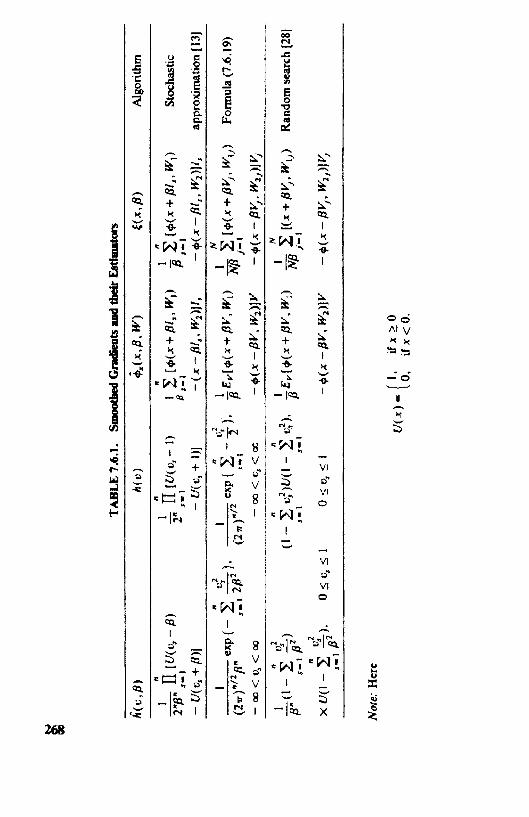
stoc
hast
ic
appr
oxim
atio
n I I
31
I Fo
rmul
a (7
.6.1
9)
Ran
dom
sear
ch [2
8]
stoc
hast
ic
appr
oxim
atio
n I I
31
I Fo
rmul
a (7
.6.1
9)
Ran
dom
sear
ch [2
8]
stoc
hast
ic
appr
oxim
atio
n I I
31
I Fo
rmul
a (7
.6.1
9)
Ran
dom
sear
ch [2
8]
stoc
hast
ic
appr
oxim
atio
n I I
31
I Fo
rmul
a (7
.6.1
9)
Ran
dom
sear
ch [2
8]
stoc
hast
ic
appr
oxim
atio
n I I
31
I Fo
rmul
a (7
.6.1
9)
Ran
dom
sear
ch [2
8]
stoc
hast
ic
appr
oxim
atio
n I I
31
I Fo
rmul
a (7
.6.1
9)
Ran
dom
sear
ch [2
8]
stoc
hast
ic
appr
oxim
atio
n I I
31
I Fo
rmul
a (7
.6.1
9)
Ran
dom
sear
ch [2
8]
stoc
hast
ic
appr
oxim
atio
n I I
31
I Fo
rmul
a (7
.6.1
9)
Ran
dom
sear
ch [2
8]
stoc
hast
ic
appr
oxim
atio
n I I
31
I Fo
rmul
a (7
.6.1
9)
Ran
dom
sear
ch [2
8]
stoc
hast
ic
appr
oxim
atio
n I I
31
I Fo
rmul
a (7
.6.1
9)
Ran
dom
sear
ch [2
8]
stoc
hast
ic
appr
oxim
atio
n I I
31
I Fo
rmul
a (7
.6.1
9)
Ran
dom
sear
ch [2
8]
stoc
hast
ic
appr
oxim
atio
n I I
31
I Fo
rmul
a (7
.6.1
9)
Ran
dom
sear
ch [2
8]
stoc
hast
ic
appr
oxim
atio
n I I
31
I Fo
rmul
a (7
.6.1
9)
Ran
dom
sear
ch [2
8]
Alg
orith
m
stoc
hast
ic
appr
oxim
atio
n [ 1
31
Form
ula (
7.6.
19)
Ran
dom
sear
ch [2
8]
Not
e: H
ere

OPTIMIZATION BY SMOOTHED FUNCTIONAIS 269
and
~ { ( S ( x * S ) , S ( x J 3 ) > ) = var [ 5 C,(x,8)] + c E [ l ( x * P ) 3 . E [ ~ ( x , p ) ] > s= I
5 u ' N - ? ~ - ~ + ( & ( x , f l ) . & ( x , 8 ) ) . (7.6.25)
Here h, , (Y) is the s t h coordinate of the vector h J V ) , ( , ) denotes the scalar product, and
u2 = n2 max sup u,'(x). (7.6.26)
Note that nz appears in (7.6.26) rather than n because of the covariance terms.
Taking into account that g(x) is bounded for all x E D and var,[+(x. W ) ] < 00, we can readily conclude that u:(x) < 00 for all x E D and therefore u2 < 00.
X E D
Now problem (7.1.16') can be solved by the following algorithm: X 1 + , = a ( x i - - a E ( x , , P , ) ) . (7.6.27)
Theorem 7.6.1 Assume that the iterative process is constructed in accor- dance with (7.6.27) and that for every x E D and for every i the following conditions are satisfied:
( ( x - - , ~ * ) , g , ( x , P , ) > 2 K,Ilx-.x*l12-YI (7.6.28)
(7 6 2 9 )
0 < a < 2K,Kc' (7.6.30)
(7.6.3 1)
(7 h.32)
ElIx,1I2 < 0 0 9 (7.6.33)
where ilx 11 = (Zt- , x ~ ) ' / ~ is the norm of x , and K, and K, are positive constants. Then process (7.6.27) converges in the mean square to the point x + , that is, lim,,,EHxi - x*1/' = 0. If we replace condition (7.6.31) by
43 I= f i j -2&.-1 < co (7.6.34) i - 1
and conditions (7.6.32) by W
Z yi<mq i - I
(7.6.35)

270 MONTE CARL0 ODTIMII^A’~ION
then process (7.6.27) converges, with probability I , to x*, that is,
Proof Without loss of generality we can set X* = 0. Taking the condi- tional expectation of ( I X , + ~ 11, given x,, . . . ,x,, we obtain from (7.6.27)
E( Itx,+ I I I 21x,, . . . . X I ) I IIXI I/ - 2a<x,, Et ( ( X I * P I > ] ) + aZE[ tC(x,,P,h CCx,.a,>>]. (7.6.36)
Substituting E [ [(x, p) ] = &.( x, P ) in (7.6.36), we obtain
E( Ii X I + I [I 21xIt. . x,) I 11 x, 11 - 2 a < x l , & ( x l , A ) ) + a 2 ~ [ < W , 7 P 1 ) , S ( x , , B , ) ) ] * (7.6.37)
Now taking (7.6.26) through (7.6.29) into account, we obtain
E(llX,+ll12 p l , . . . . x l ) 5 I I ~ , 1 l 2 - 2 ~ K 1 l I X , I l 2 + 2 w ,
+ a z 4 - ‘p,-2u2 + a2K, 11 xi 11
= ( I - 2 a K , + a 2 K 2 ) ~ ~ x l ~ ~ 2 + a Z N l ~ 5 8 , ~ 2 u 2 + 2 a y l . (7.6.38)
Taking the expectation of both sides of the last inequality, we obtain
E I [ x l+ I I[ * 2 ( I - 2 a K , + a 2 K 2 ) E )Ix, 11 + a2&-2N,-1u2 + 2 aY1
+ ( I - 2aKl + c ~ ~ K , ) ~ E 1 1 ~ , 1 1 ~ I
+ 2 (a2j3,-*N ‘az + 2ay,)(1 - 2 a ~ , + U~K,)’-~. 5 - I
(7.6.39)
I t FoIlows from (7.6.30) that I - 2aK, + a2K2 < I ; therefore (7.6.39) can be rewritten as
I
Ellx,+,l12 I K;Ellx,112 + 2 (a’#3~zNs-1u2 + Zay,)K;-’, (7.6.40) s= I
where
K3 = 1 - 2 a K , + d K 2 . (7.6.4 I )
The first term in (7.6.38) converges to 0 as i-+oo, since K,< 1 and Ell~,11~ < 00 (see (7.6.33)). Thus the theorem will be proven if we prove

OPTIMIZATION BY SMOOTHED FUNCTIONALS 27 1
that i
Iim ( ~ * P , - ’ N - I - 2 a y , ) ~ ; - ’ = 0. 1-Q) 5’1
To prove this we assume that for any number e we have chosen a number T such that, for all s > T, a2/3s-2Ns-1u2 - 2ays is less than E. Then
I T
2 (a2#3;2Ns-’u2 + 2cry,)K:-’ 5 K ; [ (a2u2/3,-2N,-1 -t ~ C X ~ , ) K ; ~ s= I Ls-I
1 I
+ x . r=T+ I
i n view of the fact that T is finite, the first term in (7.6.42) i-+ 00, since K, < 1. Using the formula for a geometrical obtain:
(7.6.42)
tends to zero as progression, we
I iim E K ~ ( I - K;-‘) limEllx,112_<IimeK; x
1 - K3 ‘+O0 s - T + I t--roc
Since E may be any positive number, wc have l im,~mEllx, 11 = 0. This completes the proof of the first part of the theorem. To prove the convergence of (7.6.27) with probability 1 , it is sufficient to
show that Zp“, , E(1l x, 11 2 , < do. Summing both sides of (7.6.40), we have by (7.6.34) and (7.6.35)
m m i
from which the result follows. Q.E.D.
Remark 1 The theorem remains valid for the deterministic optimization problem
min “g( x) = g( x*). x E D c R
which is a particular case of problem (7. I . 16). when W = 0.
Remark 2 Condition (7.6.28), together with (7.6.32), allowed g(x) to be nonconvex.

272 MONTE CARLO OPTIMIZATION
APPENDIX
Let S be a random vector uniformly distributed over the surface of a unit n-dimensional sphere with its center at origin, and let R be any given unit vector issuing from the origin (see Fig. 7.A.I).
The p.d.f. of the random angle between E and R is sought. For reasons of symmetry we confine ourselves to the semisphere 0 I cp IT. The p.d.f. is then [28]:
where
The expected value of the r.v. Q) is T E ( q ) = - 2 '
from which i t follows that on the average, R and E are orthogonal.
function, that is, It is readily verified that, as n increases, h , ( q ) approaches to Dirac's B
Fig. 7.A.2 represents h,,(q) for different n.
n . 2
- 1* 2 en1 n.
-- &. 7.A.2 The density function of cp for differ-

REFERENCES 273
EXERCISES
1 Find the efficiency C, (7.2.8) and var(coscp) of Algorithm RS-2 analytically and of Algorithm R S 5 by simulation. For Algorithm RS-5 describe the random number generator and the flow diagram of your program. 2 Prove that for a linear function g ( x ) the direction of b',= in Algorithm RS-5 (see (7.1.13)) coincides, on the average, with that of the gradient of g ( x ) .
3 By analogy with algorithm RS-1 (see (7.1.18)) describe the nonlinear tactic Algorithm RS-2, the linear tactic Algorithm RS-3, the statistical gradient Algorithm RS-5 for solving problem (7.1.16).
4 Prove that, if g(x) is convex in R" and if the point x + in which g ( x ) attains its minimum value is unique, then k( x , /I) (see (7.6. I)) is strictly convex. 5 Given a linear function ( c , x ) invariant for the convolution (7.6.1). that is, I h( 8. x - u ) ( c , u ) du = < c. x >, prove that %( x , 8) 2 g(x).
6 Prove (7.6.4) and (7.6.5).
7 Prove that, if h,(rp) - i B,,[sin"-'cp[, 0 5 cp 5 27r, then P,,(o), where c = coscp is distributed according to (7.2.12).
8 Consider the following modification of Algorithm RS-I (see (7.1.4)):
Find the efficiency C,, (7.2.8) and var(cosq), assuming that g ( x ) is a linear function.
REFERENCES
I Archetti, F., A sampling technique for global optimizstion, in Towards Global Optimlxa- tion. edited by L. C. W. Duon and G. P. &go, North Holland, American Elsevier. New Yo&, 1975.
2 Avriel, M., Nonlinear Programming. AnuryJis and Merhadr. Rentice-Hall, Englewood CliSfs, New Jersey, 1976.
3 Becker, R. W. and G. V. Lago, A global optimization algorithm, Eighth Allerton Conference on Circuits and System Ttreory, 1970, pp, 3- 13.
4 Brooks, S. H.. A discussion of random methods for gceking maxima, Oper. Res., 6, 1958,
5 Chichinadze, V. K., Random search to dettnnine the extremum of the function of several variables, Eng. Cybern., 1, 1967, 115- 123.
6 Dcvroye, L. P., On the convergence of statistical search, Inst. Elm. Electron. Eng. Tram. sysl., Man, Cybern.. 6, 1976, 46-56.
7 Dixon, L. C. W., Global optimization without convexity. Technical Report N85, The Hatficld Polytechnical Numerical Optimization Center, July 1977.
8 Dvoretzky, A., On stochastic approximation, in Proceedings of the Third Berkelq Sym- posium on Mathematical S1arislics and Probabilily, Vol. 1, 1956, pp. 39-55.
244-25 I .

274 MOW3E CARL0 OPTIMIZATION
9 LO
11
I2
13
14
15
16
17
18
19
20
21 22 23
24
25
26
27
28 29
30
Ermolyev, Yu. M., Stochastic Programming Methoa3, Nauka, Moscow, 1976 (in Russian). Ermolyev, Yu. M., On the method of generalizcd stochastic gradients and quasi-Ftjer- sequences, Cybernetics, 5, 1969, 208-220. Evtushenko. Yu. G. Numerical methods for finding global exlrema (case of a non uniform mesh). U.S.S.R. Cow. Math. Math. Phys., It, No. 6, 1971. pp. 38-55. Gaviano, M., Some general rcsuits on the convergence of random search algorithms in minimiation problems, in Toward Global Qntimizatian, cdited by L. C. W. Dixon and 0. P. Szeg&. North Holland, American Elsevier, New Yo&, 1975. Gladyshev, E. Y., On Stochastic Approximation. Theory Prob. Appl., 1966, No. 2,
Gnedenko, B. V., Sur la distribution du tcnne maximum d’une serie aleatoirc. Ann. Math., 44, 1943, 423-453. Gomulka, J., Numerical experience with Tom’s clustering algorithm and two implemcn- tations of Branin’s method, in Toward Global @timuation, Vol. 2, edited by L. C. W. Dixon and G. P. Szego. North Holland, American Elsevier, New York, 1977. liammersley, 1. M. and D. C. Handscomb, Monte Car& Methods, Wiley, New Yo&; Mcthuen. London. 1964. Katkovnik, V. Ya., Linear Esritnationt and Stochric @timiUrtion Problem, Nauka, Moscow, 1976 (in Russian). Katkovnik, V. Ya. and Yu. Kulchitsky, Convergence of a class of random search algorithms, Automat. Remote Control 1972, No. 8, 1321- 1326. Kiefer, J.. and J. Wolfowitz, Stochastic estimation of the msximum of a regression function, Ann. Math. Stat., 23, 1952, 462-466. Ktciza, V., On the modolmg of nonlinearity by the sequence of Markov chains, Liih. Math. 1.. XV, No. 4, 1975, 125-130. Mangasanan, 0. L.. Nonlinear Programming, McGraw-Hill, New York, 1969. Matyas, J., Random optimization, Automat. R e m e Contrd, 16, 1965, 246-253. Meerkov. S. M., Deceleration in the search for the global extremum of a function, A u ~ o m t . Remote Confml, 1972, No. 12, 129- 139. Metropolis, N., A. W. Rosenbluth, M. N. Rosenbluth, A. H. TeUer. and E. Teller. Equations of state calculations by fast computing machines. 1. Chem. Physics, 21. 1953,
Pincus, M., A closed form selection of certain programming problems,, Opcr. Ra., 16,
Pincus, M., A Monte-Carlo method for the approximate solution of certain types of constrained optimization probkms, Oper. Res., 18, 1970, 1225- 1228. Price, W. L., A controlled random search procedure for global optimization, in Towar& Global Optimization, Vol. 2, edited by L. C. W. Dixon and G. P. &go, North Holland, American Elsevier, New York, 1977. Rastrigin, L. A., The Stochastic Methods o/ Search, Nauka, Moscow, 1968 (in Russian). Rastrigin, L. A., and Y. Rubinstein, The comparison of the random search and the stochastic approximation wlule solving the problem of optimization, A w m r . Confd, 2,
Robins, H.. and Monro, S.. A stochastic approximation metbod, Ann. Marh. Star., 22,
272-275.
1087- 1092.
1%8,690-694.
NO. 5, IW9.23-29.
1951,400-407.

REI'ERENC'ES 275
31
32
33
34
35
36
37
38
39
40
41
42 43 44
45
46
Rubinstein, Y., Convergence of the random search algorithm, Auromaf. Control, 3, No. I,
Rubinstein, Y., Piece-wise-linear representation of function in situation of noise, Automat. Contro!, 2, No. 5, 1968, 36-42. Rubinatein, Y., choice of the optimal search strategy. J . Opfimizar. 'lirteory Appl., IS, No.
Rubinstein, Y. and J. Har-El. Optimal performane of learning automata in switched random environments, Imr. Elec. Electron. Eng. Tram. Sy$t., Man, Cyber.. SMC-7, 1977, 674- 678. Rubinstein. Y. and A. Karnovsky, Local and integral properties of a search algorithm of the stochastic approximation type. Sfmhnstic Processes Appl., 6, 1978, 129- 134. Rubinstein. Y. and 1. Weissman, The Monte-Carlo method for global optimization, Cah. Cen. Etud. Rech. Qper., 21, No. 2, 1979, 143-419. Shubert, 6. O., A sequential method for searching the global maximum of a function. Six. Indust. Appl. Math. J . Numer. AMI., 1972. No. 9, 379-388. Suitti, C., Cnnvergence proof of minimization algorithms for nonconvex functions,
Strongn, R. G., Simple search algonthm for global extremum of function of several variables and its use in functions approximation problem, Rndiofizjku, 7, No. 15, 1972,
Tom, A., A search clustering approach to the global optimization problem, in Towwdr G t W Optimixalion. Vol. 2, edited by I-. C. W. Dixon and G. P. Szcgo, North HoUand, American Elsevier, New York. 1977. Van Ryrin, J., On strong consistency of density estimations, Ann. Muth. Bar., 40, 1%9, 1765.- 1772. Venter, H. J., On estimation of the mode. Ann. Math. Stat., 38. 1%7, 1446- 1455. Wasan, M. T.. Stocliartic Approximafion. Camhridge University Pnsu. New York, 1%9. Wilde. D. J., Optimum Seeking Merho&, PrentiLmHall, Englewood Cliffs, New Jersey, 1964.
Yakowitz, S. J. and L. Fisher, On sequential search for the maximum of unknown function. J. Math. A w l . Appl., 41. 1973, 234-259. Zielinski, R., A Monte Carlo estimation of the maximum of a function. Algorithm, MI,
1969.46-49.
3. March 1976, 309-317.
JOTA. 23, 1977,203-210.
1077- 1085.
NO. 13, 1970, 5-7.


Index
Acceptance-rejection method, 45 Ahrens, J., 35, 70, 75 Antithetic variates, 135, 149, 151 Avriel, M , 234, 235, 273
Biased estimator, 145
Cheng, R,CH., 73, 75, IN, 112 6nlar, 182,231 Closed queueing network, 197 Composition method, 43 Conditional Monte Carlo, 141 Confidence interval, 187, 188 Congruential generators, 21, 22 Constrained optimization problem, 208, 259 Control variates, 126, 150, 214 Correlated sampling, 124 Crane, M. A., 183,231
Devroye, L. P.t 273 Dieter, U„ 70, 1 U Dirichlet problem, 179 Dixon, L C . W„ 252, 273 Dvorctzky, A., 240, 273
Efficiency of Monte Carlo method, 119 Eigenvalue problem, 178 Ergodic Markov chains, 160 Ermarkov, S. M„ 17, 143, 156 Estimates:
interval, 187 point, 187
Estimators: Beaie, 189 Fieller, 189 jackknife, 189 Tin, 190
Fishman, G. S., 8, 17, 73, 86, 112
Simulation and the Monte Carlo Method REUVEN Y. RUBINSTEIN
Copyright © 1981 by John Wiley & Sons, Inc.
Forsythe, GM 56, 70, 158
Gaver, D. PM 157 Generalization of von Neumann's method, 51 Generation:
beta, 80 binomial, 101 Cauchy, 91 ehi-square, 93 discrete uniform, 95 Eriang, 71 exponential, 67 extreme value, 107 gamma, 71 geometric, 104 hypcrgeometric, 106 logistic, 107 lognormal, 91 multtnormaf, 65 negative binomial, 104 normal, 86 Poisson, 102 Student, 94 Wei bull, 92
Global maximum, 234 Global optimization, 234, 252
Halton, I. H„ 156 Hammersley, I, M„ 18, 141, 156 Handscornb, D. C, I41, 156 Heidelberger, P., 192, 218, 220
Iglehart, D. L., 183, 199, 231 Importance sampling, 122 IntegraJ equations, 173 Inventory model, 230 Inverse matrix, 168 Inverse transform method, 39
277

278 INDEX
Jdhnk, M. D„ 72,81, 82
Katkovnik, Ya., 236, 274 Kicfer, JM 240, 274 Kieinen, J. P. C , 18 Knuth, D„ 31,232
Lavenburg. S* S., 126, 156,232 Law, A. M, 233 Lewis, P. A. W„ 18, 233 Linear equations, 158 Local ex trema, 234
Markov chain, 160, 185 Marsaglia, G.t 36, 70, 112 Marshal, A. W,t 156 Michailov, S. A., 18, 81, 112, 156 Mitchel, B„ 156,233 Monte Carlo integration, 115 Monte Carlo methods, 6, 11, 12 Monte Carlo optimization, 234 Multicxtremal function, 236 Multiplicative generator, 23
Naylor, 6, 8, 9, 18,36 Networks, 150 Neuts, M., 112, 156
Page, E. S-, 36, 150, 157 Pinkus, M, H , 260, 274
Queueing: Gl/G/I, 193 M/M/l , 195,230
Random quadrature method, 143 Random search algorithms, 235, 268
double trials algorithm, 236 nonlinear tactic algorithm, 237 optimum trial algorithm, 238 statistical gradient, 239
Rastrigin, L A., 236, 242t 274
Regenerative process, 184 Regenerative simulation, 184 Repairman model with spares, 195, 230 Rubinstein, Y. R., 200, 212, 233, 236, 242
Selecting best stable stochastic system, 199 Smoothed functional, 253 Smoothed gradient, 264, 266 Spanier, J., 156 Stochastic approximation, 240 Stochastic optimization problem, 258 Stopping time, 185 Stratified sampling, 131
Tests of pseudo-random numbers, 26 chi-square goodness-of-fit test, 26 Cramer-von-Mises goodness-of-fit test, 30 gap test, 32 Kolmogorov-Smirnovgoodness-oMit test, 27 maximum test, 33 run-up-and-down, 31 serial test, 30
Tocher, D. D., 19,37,90, 112 Tukey, J. WM 141
Variance reduction technique, 121,213 antithetic variate, J 35, 149, 159 common random numbers, 224 conditional Monte Carlo, 141 control variates* 126, 150, 214 correlated sampling, 124 importance sampling, 122 stratified sampling, 131
Von Neumann, J., 37, 113
Walker, A, JM 113 Wasan, M, T.f 275 Weighted Monte Carlo method, 147 Welch, P., 126 Wolfowit*, J.,240
Yakowiu, S. X, 19, 113, 147, 156

WlLEY SERIES IN PROBABILII'Y AND MATH EM AT1 CA 1, STAT1 S'I'I CS
ESTABL.ISHEL) BY WA1.TER A. St lEWI lART A N D SAMtlEL s. WILKS Editors Ralph A. Bradky J. Stuart Hunter Geo{frey S. Watson
ADLER The Geometry of Random Fields ANDERSON The Statistical Analysis of Time Series ANDERSON A n Introduction to Multivariate Statistical Analysis ARAUJO and GlNE The Central Limit Theorem for Real and Ranach
ARNOLD The Theory of Linear Models and Multivariate Analysis BARLOW, BARTHOLOMEW, BREMNER, and BRUNK Statistical
BARNETT Comparative Statistical Inference BHATTACHARYYA and JOHNSON Statistical Conceptsand Methods BI1.I-INGSLEY Probability and Measure CASSEL. SARNDAL. and WRETMAN Foundations of Inference in
DE FINETTI Theory of Probability, Volumes 1 and I I DOOB Stochastic Processes FELLER An Introduction to Probability Theory and Its Applications.
FELLER An Introduction to Probability Theory and Its Applications.
FULLER Introduction to Statistical Time SeriL% GRENANDER Abstract Inference HANNAN Multiple Time Series HANSEN. HURWITZ. and MADOW Sample Survey Methods and
Theory, Volumes 1 and I I HARDING and KENDALL Stochastic Geometry HOEL Introduction to Mathematical Statistics. Fourth Edirion HUBER Robust Statistics IOSIFESCU Finite Markov Processes and Applications ISAACSON and MADSEN Markov Chains KAGAN, LINNIK, and RAO Charactcrizdtion Problems in Mathematical
KENDALL. and HARDING Stochastic Analysis LAHA and ROHATGI Probability Theory LARSON Introduction t o Probability Theory and Statistical Inlerence.
LARSON Introduction to the Theory of Statistics LEHMANN Testing Statistical Hypotheses MATHERON Random Sets and Integral Geometry MATTHES, KERSTAN, and MECKE Infinitely Divisible Point Processes PARZEN Modern Probability Theory and Its Applications PURl and SEN Nonparametric Methods in Multivariate Analysis RANDLES and WOLFE Introduction to the Theory of Nonparametric
RAO Linear Statistical Inference and Its Applications, Second Edirion ROHATGI An Introduction to Probability Theory and Mathematical
Statistics RUBINSTEIN Simulation and The Monte Carto Method SCHEFFE The Analysis of Variance SEBER linear Regression Analysis SEN Sequential Nonparametrics: lnvariance Principles and Statistical
SERFLING Approximation Theorems of Mathematical Statistics TJUR Probability Based on Radon Measures
David G. Kendall
Probability and hfat hematirol Siati.stic.7
Valued Random Variables
Inference Under Order Restrictions
Survey Sampling
Volume I, n i r d Edirion, Revised
Volume I I . Srrond Edirion
Statistics
Second Edition
Statistics
Inference
Simulation and the Monte Carlo Method R E W E N Y. RUBINSTEIN
Copyright 0 1981 by John Wiley & Sons, Inc.

Prohutiitii,~~ onif Mutlic.*mut i d Siuiisrtcr. (CtJniinwd) WI1.L.IAMS Diffusions. Markov f’rocesses. and Martingales. Volume I :
ZACKS Thcorq of Statistical Inference
ANDERSON. AUQUIER. HAUCK, OAKES, VANDAELE. and
ARTHANARI and DODGE Mathematical Programming in Statistics BAILEY The Elements of Stochastic Processes with Applications to the
BAILEY Mathematics. Statistics and Systems for Health RARNETT Interpreting Multivariate Data BARNETT and LEWIS Outliers in Statistical Data BARTHOLOMEW Stochastic Models for Social Processes. Sewnd
BARTHOLOMEW and FORBES Statistical Techniques for Manpower
BECK and ARNOLD Parameter Estimation in Engineering and Science BELSLEY. K U H , and WELSCH Regression Diagnostics: Identifying
BENNETT and F R A N K L I N Statistical Analysis in Chemistry and the
RHAT Etements of Applied Stochastic Processes BLOOMFIELD Fourier Analysis of Time Series: An Introduction BOX R. A. Fisher, The Life of a Scientist BOX and DRAPER Evolutionary Operation: A Statistical Method for
Process Improvement BOX. HUNTER, and HUNTER Statistics for Experimenters: An
Introduction to Design, Data Analysis. and Model Huilding BROWN and HOLLANDER Statistics: A Biomedical Introduction RROWNLEE Statistical Theory and Methodology in Science and
Engineering. Sewnd Oliricin BURY Statistical Models in Applied Science CHAMBERS Computational Methods for Data Analysis C34ATTERJF.E and PRICE Regression Analysis by Example CHERNOFF and MOSES Elementary Decision Theory CHOW Analysis and Control of Dynamic Economic Systems CHOW Econometric Analysis by Control Methods CI.ELl.AND. BROWN. and dcCANl Basic Statistics with Business
COCH R A N Sampling Tcchniques. 7’hird Edition COCH R A N and COX Experimental Designs. Second Edirion CONOVER Practical Wonparametric Statistics. Secwd Eilirion CORNE1.I.. Experiments with Mixtures: Designs. Modelsand The Analysis
COX Planning of Experiments DANIEL Biostatistics: A Foundation for Analysis in the Health Sciences.
DANIEL Applications of Statistics to Industrial Experimentation DAKIEI. and WOOD Fitting Equations t o Data: Computer Analysis o f
DAVID 9 Order Statistics. Second Edirion DEMING Sample Design in Business Research DODGE and ROMlG * Sampling inspection Tables. Second Edition DRAPER and SMITH Applied Regression Analysis, Second Edition DUNN Rasic Statistics: A Primer for the Biomedical Sciences. Second
F‘oundat ions
Applied Probabilit.r and Statblirs
WEISBERG Statistical Methods for Comparative Studies
Natural Sciences
Edition
Planning
Influential Data and Sources of Collinearity
Chemical industry
Applications. Second E l i r b n
of Mixture Data
Stc-and Edifion
Multifactor Data, Second Edition
Edirion
Regression DUNK and CLARK Applied Statistics: Analysis of Variance and
ELANDT-JOHNSON Probability Models and Statistical Methods in Genetics
Analysis ELANDT-JOHNSON and JOHNSON Survival Modeis and Data
wnrinued on back

Applid 1'rohuhiiir.r and .Stuii.stinv (Con t i n i d ) FI.EISS Statistical Methods for Rates and Proportions, Srcond Edition GAi.AMROS The Asymptotic Theory of Extreme Order Statistics GIBBONS, OLKIN. and SOBEL Selectingand Ordering Populations: A
GNANADESIKAN Methodsfor Statistical Data Analysisof Multivariate
GOLDBERGER Econometric Theory GOLDSTEIN and DI LLON Discrete Discriminant Analysis GROSS and CLARK Survival Distributions: Reliability Applications in
GROSS and HARRIS Fundamentals of Queueing Theory CU PTA and PANCHAPAKESAN Multiple Decision Procedures: Theory
and Methodology of Selecting and Ranking Populations GLiTTMAN. WILKS. and HUNTER Introductory EngineeringStatistics.
Second Edition HAHN and SHAPIRO Statistical Models in Engineering HALD Statistical Tables and Formulas HALD Statistical Theory with Engineering Applications HARTIGAN Clustering Algorithms HILDEBRAND. I-AING, and ROSENTHAL Prediction Analysis of
HOEL Elementary Statistics, Fourth Edition HOLLANDER and WOLFE Nonparametric Statistical Methods JAGEKS Branching Processes with Biological Applications JESSEN Statistical Survey Techniques JOHNSON and KOTZ Distributions in Statistics
Discrete Distributions Continuous Univariate Distributions-I Continuous Univariate Distributions 2 Continuous Multivariate Distributions
New Statistical Methodology
Observations
the Biomedical Sciences
Cross Classifications
JOHNSON and KOTZ Urn Models and Their Application: An Approach
J O H N S O N and LEONE Statistics and Experimental Design in Engineer-
JUDGE. GRIFFITHS. HILL and LEE The Theory and Practice of
KALBFLEISCH and PRENTICE The Statistical Analysis of Failure
to Modern Discrete Probability Theory
ing and the Physical Sciences, Voturnes I and 11, Stwind Edition
Econometrics
Time Data KEENEY and RAIFFA Decisions with Muhiole Obicctives LANCASl ER An Introduction to Mtdical SiatistiG L.EAMER Specification Searches: Ad Hoc Inference with Nonexperi-
McNElL Interactive Data Analysis MA". SCHAFER and S1NGPIIRWALI.A Methods for Statistical
MEYER Data Analysis for Scientists and Engineers MILLER Survival Analysis MILLER, EFRON. BROWN, and MOSES Biostatistics Casebook OTNES and ENOCHSON Applied Time Series Analysis: Volume 1, Basic
OTNES and ENOCHSON Digital Time Series Analysis POLLOCK The Algebra of Econometrics PRENTER Splines and Variational Methods R A O and MlTRA Generalized Inverse of Matrices and Its Applications RIPLEY Spatial Statistics SCHUSS Theory and Applications of Stochastic Differential Equations SEAL Survival Probabilities: The Goal of Risk Theory SEARLE Linear Models SPRINGER The Algebra of Random Variables UPTON The Analysis of Cross-Tabulated Data WEISBERG Applied Linear Regression WHITTLE Optimization Under Constraints
mental Data
Analysis of' Reliability and Life Data
Techniques

Applied Prc,hahiiit,y und Sturktirs (C'onlinued) WILLIAMS A Sampler on Sampling WONNACOTT and WONNACOTT Econometrics. Second Edition WONNACOTTand WONNACOTI' * Introductory Statistics, ntirdEdiirion WONNACOTT and WONNACOTT Introductory Statistics for Business
WONNACOTT and WONNACOTT Regression: A Second Course in
ZELLNER An Introduction to Bayesian Inference in Econometrics
BARNDORFF-NIELSEN Information and Exponential Families in
BHAlTACHARYA and RAO Normal Approximation and Asymptotic
BIBBY and TOUTENBERG Prediction and improved Estimation in
RlLLlNGSLEY Convergence of Probability Measures JARDINE and SIBSON Mathematical Taxonomy KELLY Reversibility and Stochastic Networks KINGMAN Regenerative Phenomena RAKTOE. HEDAYAT, and FEDERER 0 Factorial Designs
and Economics. Second Edirbn
Statistics
Trucrs on Probabiliiy and Staristics
Statistical Theory
Expansions
Linear Models

9 ~jlllllll 780471 I/ lll~~llll 089179 Ill 11 llll/