run-up reduction through vetiver grass final report · run-up reduction through vetiver grass final...
TRANSCRIPT

Run-up Reduction through Vetiver Grass
FINAL REPORT
Auke AlgeraMSc ThesisDelft, April 2006
Delft University of TechnologyFaculty of Civil Engineering and GeosciencesSection of Hydraulic Engineering
Graduation committee:Prof. dr. ir. M.J.F. StiveIr. H.J. VerhagenDr. ir. H.L. FontijnDrs. ing. W.N.J. Ursem

.

1
Preface
PREFACE
This report is my Master thesis at the Delft University of Technology, Faculty of
Civil Engineering and Geosciences, Section of Hydraulic Engineering. The study
and the tests were performed at the university.
I sincerely hope the study and this report will help creating better and stronger
dikes. Then doing this study was not only a pleasant but also a very meaningful
period.
I want to thank my thesis committee for being a great help during this study.
Without their help and critical review I would not be able to write the report
as it is now. I also owe thanks to the people from the Laboratory for Fluid
Mechanics. During the tests they were always directly available for answering
my questions and helping me.
Delft, 2006
Auke Algera

2
Abstract
ABSTRACT
Vetiver grass is used in tropical regions to stabilize soil structures and arable
land. Because of its stiff stems and firm roots, flow velocities are reduced and
the soil retained. The application of Vetiver grass on the outer slope of a dike
is investigated in this report.
The objective is to determine the effect of Vetiver grass hedges on the run-
up. Also the effect of different planting configurations on the run-up has to be
discussed.
Different research shows that the layer thicknesses and velocities on a location
on the outer slope depend on the maximum run-up height and the height of the
location. The overtopping volumes over a dike depend mainly on the fictitious
run-up height and the crest height.
A dense hedge of Vetiver grass is able to pond water. A relationship can be
found between the water depth behind the hedge and the specific discharge
through the hedge. About the failure of Vetiver grass hedges little is known,
however research shows that a Vetiver grass hedge is able to pond water up
to 40 cm.
Tests are conducted on small-scale. Vetiver grass hedges is modelled as vertical
plates with vertical slits. The blocking factor is determined by use of the
relationship between the water depth and the specific discharge of a Vetiver
hedge. A blocking factor of 75% corresponds with a Vetiver hedge. Different
plates with different slit widths are used to determine the effect of the width
of the slits on the results.
The measures in the tests are chosen so that the dependency of the results on
the openings are is negligible. For tests it can be derived from theory that the
relative reduction of the run-up height only depends on the blocking factor.
The theory that the reduction of the run-up for the tests is independent of the
run-up height could not be rejected. The results of the tests show a constant
reduction of the overtopping volumes. The breaker parameter is important for
the reduction of the run-up height. It is assumed that the different amount
of turbulence in the run-up tip with different breaker parameter, causes the
dependency of run-up height on the breaker parameter.
With a blocking factor of 75% a reduction of the run-up volume of more than
55% is measured. A blocking factor of 60% causes a reduction of the volume
of 40%.
The flow through the openings in the tests is drag dominant. For larger run-up
the flow remains drag dominant. Thus modeling a Vetiver hedge by a plate with
larger openings is allowed.

3
Abstract
An example with the use of Vetiver grass on a dike in Vietnam is worked out.
This example shows that with the use of two Vetiver grass hedges on a dike
a reduction of 90 cm of the crest height is feasible. This corresponds with a
reduction of 20% of the costs and material use in this example.

4
Table of Contents
CONTENTS
PREFACE 1
ABSTRACT 2
1. INTRODUCTION 6
1.1 Background 6
1.1.1 The use of Vetiver grass 7
1.2 Problem Definition 9
1.3 Objective of this research 9
1.4 Outline 10
2 STATE OF THE ART 12
2.1 Wave Run-up 12
2.1.1 Wave run-up height 12
2.1.2 Layer Thicknesses and Velocities of Wave run-up 14
2.1.3 Summary and Evaluation 16
2.2 Characteristics of Vetiver Hedges 16
2.2.1 General Characteristics of Vetiver Grass 16
2.2.2 Flow Through Dense Planted Hedges 17
2.2.3 Failure of Vetiver through flow 19
2.2.4 Summary and Evaluation 20
2.3 Objects in Run-up 21
2.3.1 Flow around Objects in Run-up 21
2.4 Conclusion 23
3 SMALL-SCALE RUN-UP TESTS 24
3.1 Modeling a Vetiver Grass Hedge 24
3.1.1 The blocking-factor 25
3.2 Test Design 26
3.3 Test Procedure 28
4. RESULTS OF THE TESTS 30
4.1 Processes observed 30
4.2 Error Analysis 31
4.3 Quantitative Results 33
4.3.2 Overtopping 35
4.3.1 Run-up height 37
5. VETIVER GRASS ON A DIKE 42
5.1 Location 42
5.2 Design of the Dike 43
5.5 Construction Costs 47
5.4 Management Considerations 47
5.5 Conclusions 48

5
Table of Contents
6 CONCLUSIONS AND RECOMMENDATIONS 50
6.1 Conclusions 50
6.2 Recommendations 50
REFERENCES 52
APPENDIX 1 PROCESSING OF THE MEASUREMENTS I

Introduction
6
1. INTRODUCTION
In this chapter some background is given on the subject. From this background
a problem definition and objectives of this research are extracted. After that
the outline is given for research on Vetiver grass and run-up.
1.1 Background
A large part of the world’s human population lives along coasts and in river
deltas. These people are often protected against flooding by dikes. The most
well known failure mechanism of a dike is overflow when the water level
exceeds the dikes crest level. An overview of failure mechanisms can be seen
in figure 1.1
Fig. 1.1: Failure
mechanisms of Dikes
(TAW,1998)
The height of dikes is often determined by the permitted wave run-up and
wave overtopping discharge. Since one of the failure mechanisms of dikes is
the erosion of the inner slope, caused by wave overtopping, this should be
controlled (mode B in fig. 1.1). In the Netherlands research has been done on
overtopping and run-up in order to determine the right crest levels (van der
Meer, 2001). The crest level is an important parameter in dike design since it
has considerable influence on the materials and space required. However, to
prevent the inner slope from erosion also other measures besides raising the
dikes crest can be implemented.
Designing a berm or making the slope of the dike less steep can be effective as
wave run-up reduction. These measures are quite costly since they require a
lot of extra building material and space. Especially in densely populated areas
these measures will be very expensive.
Another way to reduce the run-up is increasing the roughness of the outer
slope. With a rough outer slope more energy will be dissipated and less water
will overtop the dike. An outer layer of rubble mound rocks can reduce the wave
run-up by 45 % compared to a smooth asphalt layer (van der Meer, 2002). An
armour layer on the inner slope of the dike will increase the permitted wave

Introduction
7
overtopping discharge since the erosion will be limited. If no rock is available
nearby this will be expensive too.
A relatively cheap armour layer can be a vegetative layer. The roots of the
vegetation will hold the soil of the dike and the part above the ground will be
able to reduce the wave run-up. The reduction of wave run-up by a field of low
grass, is small compared to a smooth slope (van der Meer, 2002). A low grass
cover on the outer and inner slope of a dike is used to control erosion, since
it can create a good closed sod. Higher vegetation like bushes and trees may
give more reduction in run-up however, uprooting or falling of a tree or bush
during a storm leaves the slope exposed, so the use of trees and bushes is
often discouraged.
Tall stiff grasses cannot get uprooted; roots of over a meter tall are common
and when loaded by a horizontal force the stems will bend before the roots
break. The stiff stems can reduce the wave run-up flow. Another advantage
of these grasses is that they may grow fast and any damage can be repaired
relatively fast compared to trees and bushes.
1.1.1 The use of Vetiver grass
Vetiver grass hedges have been used in agriculture for centuries in India and
South-east Asia. The hedges are used to protect slopes from erosion and retain
the soil and water. They are planted along the contour of the slopes and the
Vetiver roots reinforce the soil and the leaves and stems slow down the flow
and thus allow sediment to settle an example can be seen in figure 1.2. The
most used type of Vetiver grass is Vetiver Zizanioides. This is a large type of
Vetiver grass which hardly produces any seeds.
Fig. 1.2: A clump of
Vetiver grass ponding
water (Maaskant, 2005)
Vetiver grass is not the only stiff stemmed grass; some others are switch grass
(Panicum virgatum L.), miscanthus (Miscanthus sinensis) and tall fescue
(Festuca arundinacae). Below in table 1.1 some mechanical properties of the
different grasses are described.

Introduction
8
Grass M (m-2) d (mm) I (mm4) E (Gpa) MEI (N)
Switchgrass old 3700 3.15 4.8 8.5 152
Switchgrass young 7400 3.85 10.8 2.9 231
Vetiver 3500 9.10 337 2.6 3060
Miscanthus 10400 2.25 1.3 3.5 46
Fescue 6870 1.75 0.2 0.2 1
Table 1.1 Stem density,
stem diameter, moment
of inertia, modulus of
elasticity, MEI product
(Dunn, 1996)
Vetiver has some advantages compared to other tall grasses. The stems of
Vetiver have a larger diameter than other types and so a complete clump is
stiffer than the others (MEI), as can be seen in table 1.1. Vetiver also has a
vigorous root system. A biological advantage of this type of Vetiver grass is
that it is not invasive, which means that when you plant it, it will not become
a weed because it is sterile. Vetiver is fast growing compared to the other
grasses, under ideal circumstances Vetiver stems can grow over 1 cm per day
(Maaskant, 2005). Vetiver grows under a wide variety of site conditions. Vetiver
is hardly eaten by cattle so grazing on an area will not affect the hedges.
The grass cannot stand severe frost so its use is limited to tropical and sub-
tropical regions. Vetiver is currently used in many countries of the world for
the retention of soils in agricultural areas and the stabilization of soil structures
(see figure 1.3)
Vetiver is for instance currently used for bank stabilization in Vietnam (figure
1.4), to protect roadsides from erosion in China and stabilize hill slopes in
South America. Since it has a lot of engineering applications some research
has already been done on the characteristics of the stems and the roots of the
grass. Because of its mechanical and biological characteristics and the fact that
knowledge about maintenance and planting of Vetiver is available in a lot of
countries, Vetiver grass is the prime candidate for the reduction of run-up.

Introduction
9
1.2 Problem Definition
Overtopping of waves may cause erosion of the inner slope and therefore
weaken the dike. Vetiver hedges on the outer slope may decrease the run-
up that is causing the overtopping. Using Vetiver may reduce material costs,
construction costs and the required space to build a dike. Further research
is necessary, before Vetiver grass hedges can be used to decrease the wave
overtopping. The hedges on the dikes may protect large areas against flooding
and therefore have to be reliable during storm events. Research has to be done
in the field of performance, maintenance and construction before Vetiver can
be relied on. One of the most important things that has to be investigated is
the amount of reduction of wave run-up due to Vetiver grass hedges. The wave
run-up levels can be used to determine the overtopping.
1.3 Objective of this research
The main objective of this research is:
“Determine the effect of Vetiver grass hedges on wave run-up”
A relation has to be found between the wave height, hedge characteristics
and run-up level. The following questions related to this objective will be
answered:
• What is the hydraulic resistance of Vetiver grass hedges?
• What is the effect of different planting configurations on the reduction of
the wave run-up?
Related problems like failure of the grass due to overloading will be briefly
mentioned in this report.

Introduction
10
1.4 Outline
In this report first attention is paid to what is already known about Vetiver grass
and run-up. This is described in chapter 2 “State of the art”. In this chapter
finally conclusions are drawn, about what subjects need further investigation. In
chapter 3 “Small scale tests” tests are described to test the hydraulic resistance
of Vetiver grass in wave run-up. These tests are conducted and the results are
presented in chapter 4 “Results”. The conclusions from chapter 4 are used to
work out an example of real Vetiver on a dike. The effect of Vetiver on the
construction costs and material use can be seen in chapter 5 “Vetiver on a
dike”. Conclusions and recommendations for further research are finishing this
report in chapter 6.

.

12
State of the Art
2 STATE OF THE ART
In this chapter characteristics of wave run-up and Vetiver grass are discussed
as far as they are useful for determining the reduction of the run-up. From the
known characteristics of the wave run-up and Vetiver conclusions will be drawn
on what needs to be tested furthermore.
2.1 Wave Run-up
A breaking wave on a slope of the dike causes a layer of water to run-up on the
dike. For calculations on the reduction of the wave run-up the height, the layer
thicknesses and velocities have to be known for a smooth slope.
Figure 2.1 Definition
sketch for wave run-
up
2.1.1 Wave run-up height
The wave run-up height has been a subject to a lot of research, since it is an
important parameter for the design of dikes and breakwaters. For the calculation
of wave run-up heights of regular breaking waves on smooth slopes research
has been done by Hunt and Schüttrumpf.
Regular waves
Hunt’s Formula
Hunt’s formula gives for regular breaking waves ( ξ ≤ 2 5, ):
R H
H
L
u =
=
ξ
ξαtan
0
Equation 2.1
The run-up is maximum at ξ ≈ 3 just at the transition between plunging and
collapsing.
Schüttrumpf, 2001
Schüttrumpf proposes the following formula for breaking and non-breaking
regular waves:

13
State of the Art
Equation 2.2 R H c c
c
c
u = ⋅ ⋅ ⋅=
=
1 1
1
1
2 25
0 5
tanh( )
,
,
*
*
ξ
The advantage of this formula is the smooth transition between breaking and
non-breaking waves in one formula.
Random waves
Van der Meer, 2001
For wave spectra van der Meer gives for waves on a dike or breakwater the
following formula. It is used for the design of dikes in the Netherlands:
R Hu m b f2 0 01 65% / ,= ⋅ ⋅ ⋅ ⋅γ γ γ ξβ
With a maximum for larger ξ0
Equation 2.3
R Hu m f2 0 04 0 1 5% / ( , , / )= ⋅ ⋅ −γ γ ξβ
Where:
Ru2% = 2% wave run-up level above the still water line (m)
Hm0 = wave height H mm0 04= ⋅ (m)
γ b = the influence of a berm (-)
γ f = the influence of the roughness of the slope (-)
γ β = the influence of oblique wave attack (-)
ξ0 = the surf similarity parameter ξ α0 0= tan / s (-)
s0 = wave steepness s H gTm m0 0 1 0
22= ⋅ ⋅ −π /( ), (-)
Tm−1 0, = spectral wave period T m mm− −=1 0 1 0, / (s)
m0 = zero moment of spectrum (m2)
m−1 = first negative moment of spectrum (m2s)
This formula represents the average wave run-up level and is different from the
design rule. This formula includes the influences of a berm and the roughness
of the slope. The reduction of the Vetiver grass on the wave run-up could to be
implemented in one of these factors. The wave spectrum that has to be used to
calculate the wave run-up is the wave spectrum at the toe of the dike.
Van Gent, 2002
Van Gent proposes the following formula for the wave run-up:

14
State of the Art
R H c p
R H cc
p
c
u m
u m
2 0 2 0 0
2 0 34
0
0
2 1 35
%
%
/
/
.
= ⋅ ≤
= − ≥
=
ξ ξ
ξξ
c
cc
cp
c
c
3
43
2
2
3
2
4 0
0 25 0 5
=
= ⋅ = ⋅
.
. .
Equation 2.4
The advantage of this formula is that the transition of breaking to non-breaking
is fluent, still two equations are used.
Schüttrumpf, 2001
Schüttrumpf uses one equation to describe the relationship between the run-up
height and the ξd for wave spectra. This is another ξ than used by van Gent and
van der Meer. To calculate L0 Schüttrumpf used the average period instead of
the Tm-1,0
. ξ0 is about 5% smaller than ξ
d in general.
R H c c
c
c
u s d2 1 1
1
1
3 0
0 65
%
*
*
tanh( )
,
,
= ⋅ ⋅ ⋅
=
=
ξEquation 2.5
2.1.2 Layer Thicknesses and Velocities of Wave run-up
Research done on flow on dike slopes was done to determine the wave
overtopping rates. No significant difference in the layer thickness and run-up
velocity between model tests with and without wave overtopping could be found
(Schüttrumpf, 2001). Most investigations on velocities and layer thicknesses
find the following relationships between run-up and thickness or velocities.
Equation 2.6 u c g R zu u= ⋅ ⋅ −( )
Equation 2.7h c R zh u= ⋅ −( )
In these equations z is the height on the slope. and ch and c
u are constants
Regular Waves
For regular waves Schüttrumpf, 2001 finds ch = 0.284. This author conducted
tests with slope angles of 1:3, 1:4 and 1:6. According to Schüttrumpf, 2001 this
value is in good accordance with observations by Tautenhain (ch = 0.246). For
cu a value of 0.94 is proposed. R
u was calculated by using equation 2.2
Random Waves
The following formulae were proposed by Schüttrumpf and van Gent, 2003 for
the layer thicknesses and velocities for wave spectra:
15
State of the Art
u
g Hc
R z
Hs
uu
s
22
2%%
%
⋅= ⋅
−
Equation 2.8
h
Hc
R z
Hs
hu
s
22
2%%
%= ⋅−
Equation 2.9
q c g R zq u2 2 2
1 5
% % %
.= ⋅ ⋅ −( )Equation 2.10
Where:
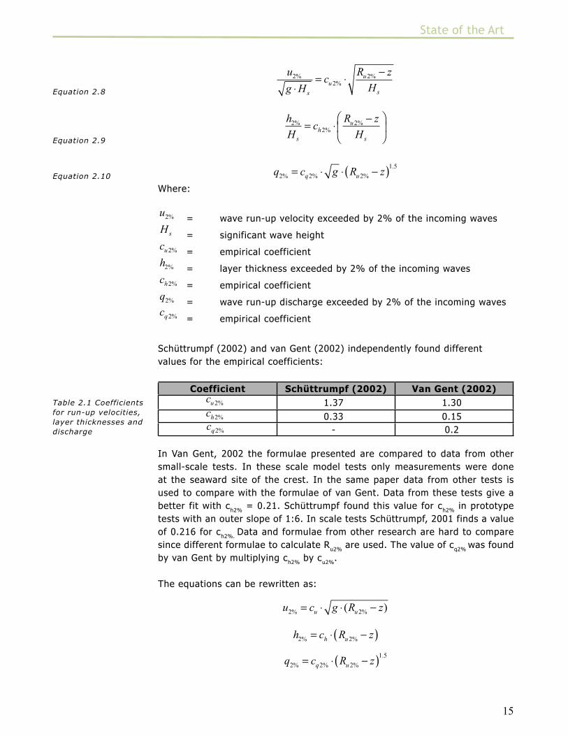
u2% = wave run-up velocity exceeded by 2% of the incoming wavesH s = significant wave heightcu2% = empirical coefficienth2% = layer thickness exceeded by 2% of the incoming wavesch2% = empirical coefficientq2% = wave run-up discharge exceeded by 2% of the incoming wavescq2% = empirical coefficient
Schüttrumpf (2002) and van Gent (2002) independently found different
values for the empirical coefficients:
Coefficient Schüttrumpf (2002) Van Gent (2002)cu2% 1.37 1.30ch2% 0.33 0.15cq2% - 0.2
Table 2.1 Coefficients
for run-up velocities,
layer thicknesses and
discharge
In Van Gent, 2002 the formulae presented are compared to data from other
small-scale tests. In these scale model tests only measurements were done
at the seaward site of the crest. In the same paper data from other tests is
used to compare with the formulae of van Gent. Data from these tests give a
better fit with ch2%
= 0.21. Schüttrumpf found this value for ch2%
in prototype
tests with an outer slope of 1:6. In scale tests Schüttrumpf, 2001 finds a value
of 0.216 for ch2%.
Data and formulae from other research are hard to compare
since different formulae to calculate Ru2%
are used. The value of cq2%
was found
by van Gent by multiplying ch2%
by cu2%
.
The equations can be rewritten as:
u c g R zu u2 2% %( )= ⋅ ⋅ −
h c R zh u2 2% %= ⋅ −( )
q c R zq u2 2 2
1 5
% % %
.= ⋅ −( )

16
State of the Art
u2%
, c2%,
q2%
are dependent on Ru2%
and therefore the values for regular waves
and wave spectra can be compared. It may not be necessarily true that for every
wave in a wave spectrum that has a run-up height of Ru2%
also the velocities
and layer thicknesses measured are of the value u2%
and h2%.
However, these
values are strongly correlated. Therefore the values of ch2%
and cu2%
can be
compared to ch and c
u.
2.1.3 Summary and Evaluation
For the run-up levels the following graphs compare the different researches
about this subject.
Figure 2.2 Wave run-
up levels according to
different research
Differences in the results can be explained by different scales (see chapter
3 and 4), different measurement techniques and the fact that these highly
turbulent flows are difficult to measure. Schüttrumpf, 2001 finds a slightly
lower value for the run-up levels than the other studies for regular waves. Also
lower velocities and quite large layer thicknesses were found relative to other
research. Since Schüttrumpf, 2001 is the only study found with systematic
measurements of run-up levels, velocities and layer thicknesses for regular
waves, these results are used for further calculation.
2.2 Characteristics of Vetiver Hedges
In this section the mechanical and hydraulic characteristics of Vetiver grass will
be discussed. In order to get a good view on how Vetiver grass may reduce
the run-up and handles with the loads. A lot of research has been done to
derive the resistance of flow through vegetated channels (Ben Chie Yen, 2002).
However, most of the research has been done for submerged vegetation and
with open channel flow. The research is focused on finding resistance factors in
order to find the resistance for the whole lining. A Vetiver hedge on the other
hand is a discrete object in flow.
2.2.1 General Characteristics of Vetiver Grass
Vetiver grass is a stiff stemmed grass. Dunn, 1996 investigated the mechanical
properties of three types of stems (vegetative stems, green internodes, dry
internodes) of the grass and came up with the values below:

17
State of the Art
Veg. stems Gr. internodes Dry internodes
Largest Diameter 4.5 mm 8.6 mm 6.2 mm
Smallest Diameter 1.6 mm 6.1 mm 4.9 mm
Mom. of Inertia (Major Axis) 8.2 mm4 272 mm4 83 mm4
Mom. of Inertia (Minor Axis) 1.0 mm4 120 mm4 45 mm4
Modulus of Elasticity E 0.21 GPa 2.6 GPa 4.7 GPa
Bending Angle Yield Point φ 5.1 º 2.4 º 5.6 º
Yield Strength Y 3.7 MPa 7.3 MPa 20.2 MPa
Table 2.2 Mechanical
characteristics of
Vetiver grass (after
Dunn, 1996)
The different stems of the plant grow very dense. Meyer et al., 1995 report
3500 stems per m2. He reported a diameter of 9.1 mm which is combined stem
and leaves. Rough calculations show that 22.7% of the total surface is taken
by stems.
2.2.2 Flow Through Dense Planted Hedges
Some tests have been performed with dense planted hedges of Vetiver. The
small slips of Vetiver were planted less than 15 cm apart. The result after some
time is a very dense hedge which is able to pond water. Flow through a discrete
Vetiver grass hedge is drawn in figure 2.3
Figure 2.3 Flow through
a discrete Vetiver
hedges
Dabney, 2003
In order to find a relationship between the discharge and the backwater depth,
in Metcalfe (2003) and Dabney (2003) it is tried to determine a Manning’s ‘n’
for the resistance of a barrier of Vetiver grass. Manning’s equation is commonly
used for determining the resistance for water flowing through vegetation lined
channels:
Equation 2.11
Where:
= the velocity in this case u1
= a hydraulic resistance parameter
= the hydraulic radius
= the slope of the bottom
For the hydraulic radius of wide flows, the backwater depths are used. This
however, is not useful in this case since the backwater depth is independent of
the slope (Dabney, 1996). The ‘n’ depends on the specific discharge. However,

18
State of the Art
the Manning’s ‘n’ values may serve as indicative values for the backwater depth,
only for the slopes tested, which are slopes in the range of 0.03-0.07.
Figure 2.4 ‘n’-values
for different vegetation
versus specific discharge
(Dabney, 2003)
Metcalfe, 2003
In Metcalfe (2003) ‘n’ values of about 0.6 s/m1/3 were found for hedges of 2
years old with a maximum discharge of 0.06 m2/s. Also higher values for lower
discharges were found which compare good with the values in Dabney, 2003.
Dalton, 1996
In Dalton, 1996 the following formula is derived after Smith, 1982:
q x z za b= ⋅ ⋅1 ∆Equation 2.12
The coefficients ξ, a and b were determined by the use of linear regression
analysis. The tests were done on seedlings planted in one row with a space of
125 mm with hedges of different ages. For a hedge of 2 years old the following
constants were found:
x
a
b
===
0 66
1 78
0 62
.
.
.
For all the heights in meters and q is in m2/s
Dabney, 1996
Dabney (1996) only provides a formula without test results or theoretical
considerations.

19
State of the Art
∆
∆
d Re Veg Leaf Re
d
= ⋅ ⋅ ⋅ <
= ⋅
0 000341 11 700
0 0762
1 07 0 17 0 47. ,
.
. . ,
RRe Veg Leaf Re0 49 0 17 0 47 11 700. . , ,⋅ ⋅ > Equation 2.14
In which
Re = the Reynolds Number q /ν (-)
(-)
= The diameter of the stem measured at 5 cm height (cm)
= Number of stems per cm2 at 5 cm height (cm-2)
= The width of the hedges (cm)
= A dimensionless number related to the number of leaves (-)
For the larger Reynolds number this formula can be rewritten as:
qVeg Leaf
d=⋅ ⋅
⋅ν
0 0762 0 35 0 96
2 04
. . .
.∆
In this formula apparently no difference is made between the difference in
water level and the water level upstream.
2.2.3 Failure of Vetiver through flow
No specific research has been done about the failure of whole hedges. The
failure occurs because of the overloading of a single stem. When stems are
loaded, they first bend through an elastic range and then an inelastic range.
After that the stems will fail and the stems may break or bend and develop a
hinge point (Dunn, 1996 after Rehkugler and Buchele). Because of interactions
between the stems in a hedge a single plant failure is hard to calculate from
the mechanical properties of a single stem.
Dabney, 1996 report backwater depths up to 0.4 m for Vetiver grass hedges of
0.3 m wide. Meyer, 1995 reports a backwater depth of 0.42 m. Dabney, 1996
also argued that the failure of grass hedges depend on the density of the hedge.
A dense hedge will fail with lower discharge because of the higher backwater
depth. Sediment and residues will weaken a hedge even more because of
filling up the hedge, while not adding to the strength. In Meyer, 1995 tests
were performed to determine the sediment trapping capacity for several types
of grass hedges. Those tests were carried out in a small indoor flume and
the influence of placing the grass in the flume is unknown. It was found that
the sediment increased the backwater depth, because the sediment trapped
blocked the openings in the hedges. In Temple, 2001 tests with switch grass
and water with flowing residues were performed. The result was a weaker
hedge because the residues blocked the flow and a higher backwater with
lower discharge was the result. With wave run-up however this will not be an

20
State of the Art
issue because of the oscillatory flow.
For single plants of Vetiver grass Chengchun Ke, (2002) reports the ability to
remain erect in flows of 0.6-0.8 m deep with velocities up to 3.5 m/s. No other
reports on the hydraulic characteristics of single plants could be found.
2.2.4 Summary and Evaluation
The different formulae for the flow through hedges are presented in figure
2.5.
Figure 2.5 backwater
specific discharge
relationships
The backwater discharge relationships show remarkable similarities. This is
mainly because of the fact that the hedges are all tested under the same flow
regimes and the formulas are found by curve fitting. The formula of Dabney,
2003 can only be used for the slopes tested since the backwaterdepth is
independent of the slope. The use of Manning’s formula is not appropriate
for a situation with a discrete hedge. Dabney, 1996 does not present any
theoretical background or measurements. After personal communication no
further information on equation 2.14 could be presented, therefore this formula
should be used with great care. In the following chapters the formula presented
by Dalton, 1996 will be used. Some some remarks about the values of x, a and
b are made below.
The formula presented by Dalton can be theoretically explained as follows: The
energy loss (ς) through the hedge can be calculated as follows:
du
gd
u
g1
1
2
22
2
2 2+
⋅− −
⋅= ςEquation 2.15
From this formula the following can be derived:
Equation 2.16q d g d d u= ⋅ ⋅ ⋅ − + − +2 1 2 1
22 ( )ς

21
State of the Art
For very close hedges will be very small and the term can be neglected.
Since the ς also depends on the velocities, this formula can be rewritten as:
q d g d d= ⋅ ⋅ ⋅ ⋅ −2 1 22ζ ( )
The resulting formula is similar to an equation for a submerged orifice. The ζ
in this equation depends on the elasticity and diameter of the stems, the width
of the hedge, the density and the water depth. This because the characteristics
of the hedge change with the height. Since the stems of Vetiver remain largely
erect during flow (Dalton, 1996) the effect of the bending of the stems on ζ can
be neglected. For calculations on hedges the following formula is proposed.
q d g d da= ⋅ ⋅ ⋅ ⋅ −1 1 2
0 52ψ ( ( )) .Equation 2.17
Where:
ψ = a hedge factor only dependent on the hedge characteristics
= a factor to be determined by experiments
Dalton, 1996 found a slightly higher exponent than the 0.5 mentioned in the
formula. This is mainly because of the curve fitting, because a slightly higher
value for a and an exponent of 0.5 will give almost the same results.
It has to be noted that when the flow downstream of the hedge is super-
critical, which is actually the case for figure 2.5, theoretical the downstream
water depth has no influence on the flow through the hedge.
2.3 Objects in Run-up
The only research that could be found on forces on objects in the run-up
zone on dikes and slopes was about the forces acting on a crown-wall of a
breakwater. In tests with rough slopes usually only the reduction in run-up is
measured for random or regular placed blocks or stones. However, for a slender
object protruding the run-up flow on dikes and breakwaters no literature could
be found.
To get more information about the effect of a hedge on the run-up first one
slender object is considered below. To determine the effect of one object in the
run-up zone the energydissipation has to be determined. The exact values of
the layer thickness and velocities are hard to determine as can be concluded
from the different results from van Gent and Schuttrumpf. Therefore the exact
values of the energy loss are also hard to find. However, as a first indication
the parameters that determine the energyloss can be determined.

22
State of the Art
2.3.1 Flow around Objects in Run-up
The resistance of one object is causing the dissipation of energy of the flow.
Therefore the forces on a object are important for the reduction of the run-
up. The forces per unit length on a stiff object in non-stationary flow can be
described by the Morrison-equation:
F t C AdU
dtC D U Um d( ) = ⋅ ⋅ ⋅ + ⋅ ⋅ ⋅ ⋅ ⋅0
1
2ρ ρ [kN/m]
Equation 2.18
Flow in run-up can be described as follows:
u z g R z
dz
dtg R z
Tg
g R z
bore u
u
r u
( ) ~ ( )
~ ( ( ))
~ ( )
.
⋅ −
−
⋅ −
0 5
2
Equation 2.19 [m/s]
[m/s2]
[s]
In this Tr is the run-up time, the time between the run-up bore hitting the object
and the time for the maximum run-up for the undisturbed situation. Schüttrumpf,
2001 states that the bore velocities near the vicinity of the maximum run-up-
level cannot be described by u g R zbore u~ ( )⋅ − because of viscous effects. This
is assumed to be insignificant for large waves in nature. Since Tr and u depend
on (Ru-z) the acceleration also depends on (R
u-z).
Equation 2.20
du
dtf u T
F f t T U Ddu
dth
r
r
=
=
( , )
( , , , , , , , )ρ ν
For run-up this eventually comes down to:
Equation 2.21 F f t R z g Du= −( , ( ), , , , )ρ ν
Since we are interested in the energy loss for one run-up period, we have to
integrate over Tr
and multiply by U this gives:
Equation 2.22 ∆E f g R z Du= −( , ( ), , , )ρ ν
It can be seen that the dissipation of energy depend on two geometrical
parameters that is, D and (Ru-z). The energy dissipation can be made
dimensionless by dimensional reasoning:
Equation 2.23 ∆E
g R z Df
g R z D R z
Du
u u
ρ ν⋅ ⋅ − ⋅=
⋅ − ⋅ −
( )
( ),( )
3
From this it can be seen that the energy dissipation in one wave run-up cycle
depends on the Reynolds number and a dimensionless run-up height parameter.

23
State of the Art
The run-up parameter can be compared to the Keulegan-Carpenter number for
sinusoidal motion:
Equation 2.24
For run-up this comes down to:
Equation 2.25 U T
D
g R zg
g R z
D
R z
D
bore r
u u
u⋅=
⋅ − ⋅ ⋅ ⋅ −=
−( ) ( )
( )
2
However, it is noted that the Keulegan-Carpenter parameter is defined over
the whole wave cycle while the run-up height parameter is defined over the
run-up period only. The Keulegan-Carpenter parameter is used to determine
the energy loss per unit length of the object. Since the water depth for run-up
depends on (Ru-z) this is not necessary for run-up.
In reality the run-up height is not only dependent on the amount of energy
but also on the momentum. A crown wall on a breakwater for instance is not
reducing run-up because of energy dissipation but because of reflecting the
incoming wave. The exchange of momentum however, is also dependent on the
same two dimensionless parameters. For a hedge the different stems interact
and tests cannot be done with one stem and then simply multiplied therefore
run-up tests will be necessary.
2.4 Conclusion
From literature good information could be found on the wave run-up on smooth
slopes and on the hydraulic behavior of Vetiver hedges in stationary flow. More
research will be needed on:
• Failure of Vetiver in flow
• Peak forces acting on Vetiver in run-up
• The effect of Vetiver hedges on run-up heights and flow.
To do research on the failure of Vetiver in flow, prototype tests are needed.
The complex interactions between stiff stems and leaves are hard to scale.
Therefore real Vetiver plants need to be tested. Since full-scale run-up tests
are quite expensive, flumes could be used where the loading is represented by
a hydraulic jump. Layer thickness, celerity and bore wedge angle need to be
the same as with run-up.
To test the reduction of Vetiver hedges on run-up scale tests can be conducted.
The hydraulic characteristics of the Vetiver hedges can be scaled, except for
failure. The hedges can be represented by scaled artificial objects.
24
Small-scale Run-up Test
3 SMALL-SCALE RUN-UP TESTS
In order to determine the effect of a Vetiver grass hedge on the run-up, small
scale run-up tests have to be conducted. The tests are used to determine the
effect of a Vetiver grass hedge on:
• Run-up height
• The amount of water flowing through the hedge
In this chapter the design of the test and the scaling of the Vetiver grass hedge
is described. For run-up tests, scaling according Froudes law is used, since a
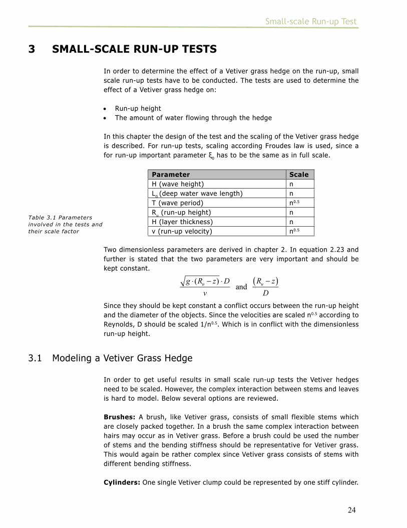
for run-up important parameter ξ0 has to be the same as in full scale.
Parameter Scale
H (wave height) n
L0 (deep water wave length) n
T (wave period) n0.5
Ru (run-up height) n
H (layer thickness) n
v (run-up velocity) n0.5
Two dimensionless parameters are derived in chapter 2. In equation 2.23 and
further is stated that the two parameters are very important and should be
kept constant.
g R z D
v
R z
D
u u⋅ − ⋅ −( )( ) and
Since they should be kept constant a conflict occurs between the run-up height
and the diameter of the objects. Since the velocities are scaled n0.5 according to
Reynolds, D should be scaled 1/n0.5. Which is in conflict with the dimensionless
run-up height.
3.1 Modeling a Vetiver Grass Hedge
In order to get useful results in small scale run-up tests the Vetiver hedges
need to be scaled. However, the complex interaction between stems and leaves
is hard to model. Below several options are reviewed.
Brushes: A brush, like Vetiver grass, consists of small flexible stems which
are closely packed together. In a brush the same complex interaction between
hairs may occur as in Vetiver grass. Before a brush could be used the number
of stems and the bending stiffness should be representative for Vetiver grass.
This would again be rather complex since Vetiver grass consists of stems with
different bending stiffness.
Cylinders: One single Vetiver clump could be represented by one stiff cylinder.
Table 3.1 Parameters
involved in the tests and
their scale factor

25
Small-scale Run-up Test
This would neglect the bending of Vetiver grass. However, as said in chapter 2,
the effect of bending can be neglected. The drag factor of a cylinder however,
is not constant. The drag factor is related to the Reynolds number. Since we do
not know the velocities between closely packed cylinders the drag is hard to
determine and is not representative for a Vetiver clump.
Vertical plate with openings: A plate with openings can also represent a
hedge of Vetiver grass. The openings in the plate should represent the openings
in a Vetiver hedge. This can be established by using the stage-discharge
relationship of a Vetiver grass hedge described in chapter two. Again problems
may occur because of laminar flow through the openings.
3.1.1 The blocking-factor
A vertical plate on the dike slope is used to model the Vetiver hedge. Vertical
slits in the plate have to be cut so the plate is hydraulically representative for
a Vetiver hedge.
The blocking factor of the Vetiver hedges is calculated as follows. From the
stage discharge graph a specific discharge of 0.08 m2/s is found at a water
level of 0.4 m in front of the hedge. The discharge through a contraction of a
channel is calculated using the following formula:
q b d g d= ⋅ ⋅ ⋅ ⋅ ⋅ ⋅µ2
3
2
3Equation 3.1
μ is the contraction coefficient and depends on the blocking factor, Froude
number and the width of the sheet. From Kindsvater an Carter, 1953 an
average value of 0.7 for μ is found. For q = 0.08 m2/s and d = 0.4 m a value
for b is found of 0.25. Hence the blocking factor of the Vetiver grass is 75
%. By planting Vetiver in a wider grid or overloading a hedge lower blocking
factors could be obtained. Therefore tests with different blocking factors are
conducted: 75 % and 60 %.
Figure 3.1 Water level
discharge graph for
Vetiver hedges and
different blocking factors

26
Small-scale Run-up Test
3.1.2 Distribution of the slits
Making the slits too small would overestimate the reduction of run-up because
of laminar flow through the slits. This is inevitable since the flow is oscillatory
and the velocities are near zero near the moment of maximum run-up. The
effect of this can be reduced by creating wider slits.
Making the slits too wide would also overestimate the reduction of the run-
up. In front of a Vetiver hedge the water surface is assumed horizontal along
the hedge. The openings in the hedge are too small to get large differences
in water level along the hedge. With very wide gaps in the plates flow in the
middle of the gaps is not affected by the blocking on the sides. In figure 3.1 the
different flow profiles through the different opening width presented
Figure 3.1 Flow profiles
through openings in the
hedge.
Only for the middle turbulent flow profile hardly any wall effects occur. Because
the flow profile and velocities are hard to determine several distributions of
slits were tested in a wave flume of 80 cm wide. The results for the different
plates with the same blocking factor can only be similar, when the middle flow
profile is mainly present.
The same flow profile is obtained in stationary flow. The blocking factor of 75
percent resembles vetiver in stationary flow. Given the rectangular flow profile
the flow through the openings can be considered quasi-steady. And so a plate
with slits may resemble a vetiver hedge very well in run-up.
Name Blocking Number of slits Width of slits Spacing
A 0% 1 80 cm -
B 75% 8 2.5 cm 10 cm
C 75% 4 5 cm 20 cm
D 60% 16 2 cm 5 cm
E 60% 8 4 cm 10 cm
F 60% 4 8 cm 20 cm
Table 3.2 Table with
different hedges tested.
Hedges with two
different blocking factors
were used.
3.2 Test Design
For the dike a slope of 1:3 is designed since this is a common slope angle for
dikes. Run-up is measured by placing another slope 1:3 behind the hedge and
measuring the run-up height. In figure 3.3 the test set-up is shown:

27
Small-scale Run-up Test
Figure 3.3 Test set-up
used to measure the
reduction of the run-up.
The amount of water passing through the hedge is determined by putting a box
behind the hedge and measuring the amount of water of a controlled number
of waves.
Figure 3.4 Test set-
up used to measure
the reduction of the
overtopping.
For the slope and the vertical plates laminated wooden sheets of 18 mm
are used. Each of the different plates is tested for 6 different regular wave
climates:
Table 3.3 Waves used for
testing.Vmax
is calculated
by using 0.94 for cu this is
proposed by Schüttrumpf
(2001) see chapter 2
Nr. H T L0
ξ Ru
(Hunt) Vmax
1 125 mm. 2.28 s 8.1 m 2.7 0.34 m 1.10 m/s
2 128 mm. 2.5 s 9.7 m 2.9 0.37 m 1.25 m/s
3 135 mm. 2.5 s 9.7 m 2.8 0.38 m 2.03 m/s
5 150 mm. 2.5 s 9.7 m 2.7 0.40 m. 1.32 m/s
4 140 mm. 2.70 s 11.3 m 3 0.42 m 1.23 m/s
6 160 mm. 2.88 s 12.95 m 3 0.48 m 1.50 m/s
For some plates additional tests were conducted with other waves these are
shown in table 3.4
Nr. H T L0
ξ Ru
(Hunt) Vmax
7 0.12 2.08 6.75 2.5 0.3 0.99
8 0.14 2.25 7.90 2.5 0.35 1.21
9 0.16 2.4 8.98 2.5 0.4 1.4Table 3.4 Waves used for
testing.
In table 3.5 the plates with different blocking factors are described. The
maximum Reynolds number given is for waves of 0.1 m which generate a flow
through the slits. Using higher waves will give even higher Reynolds numbers.

28
Small-scale Run-up Test
Name Blocking No. of slits Width of slits (Ru-z)/D Re
max,1
A 0% 1 80 cm - 8.8*105
B 75% 8 2.5 cm 1.7 2.7*104
C 75% 4 5 cm 0.85 5.5*104
D 60% 16 2 cm 3.4 2.2*104
E 60% 8 4 cm 1.7 4.4*104
F 60% 4 8 cm 0.85 8.8*104
Table 3.5 The hedges
and the Reynolds number
and dimensionless run-
up number. (Ru-z)/D
is calculated for the
smallest wave. Remax,1
is
calculated by using the
max. velocity from the
first wave and the width
of the slits
The Reynolds numbers seem high enough to ensure turbulent flow. However,
these are calculated by the velocities of the undisturbed run-up. The hedge
itself will slow down the run-up velocities and pond water.
3.3 Test Procedure
The run-up is measured by use of a point gauge. A series of waves are monitored
and the average run-up of the regular waves is being used. A picture of the
upper part of the slope is visible in figure 5.3.
Figure 3.5 A Picture of
the test set-up. Looking
down from the crest. The
point gauge for measuring
the run-up level and the
hedge behind the plate is
clearly visible. This part
of the slope could be
removed to measure the
overtopping
The amount of water flowing through the hedges is measured by collecting water
that is passing through the hedge in a box. This is established by removing
the slope above the hedge. First the wave generator was started so no start
effects would be measured. When a controlled number of waves passed the
hedges, first the box was closed than the wave generator was stopped. The
water collected in the box was pumped in another box that could be weighed
in order to determine the amount of water.

29
Small-scale Run-up Test
Figure 3.6 The box that
was used to collect the
water. The pump was
used to pump water to a
weighing device. In the
background the hedge is
visible.

30
Test Results
4. RESULTS OF THE TESTS
The results of the tests conducted are presented here. First the general
processes observed are discussed. This is a description of how a Vetiver hedge
is reducing the run-up. Then an error analysis is described before the measured
results are presented.
4.1 Processes observed
When the run-up tongue is hitting the Vetiver hedge, part of the water is
blocked so the run-up is reduced. This is off course the most important part of
the reduction of the run-up. (see figure 4.1)
Figure 4.1 Side view of
the run-up bore hitting
the hedge. (behind the
measuring tape). The
water is partly splashing
up against the hedge and
partly transmitted.
The water that is blocked by the hedge creates a reflected wave from the hedge.
(see figure 4.2) This wave is running down the slope to the water. Breaking of
a wave is related to the steepness of the water surface. This is caused by the
combination of the incoming and reflected wave. Since the hedge is altering
the reflected wave, the breaking is also changed. The change of the breaking is
determined by the breaker parameter (ξ) and the dimensionless run-up height
(Ru/z).

31
Test Results
Figure 4.2 Side view of
the reflected wave of
the run-up bore. The
maximum run-up level
has not yet been reached.
Yet a wave on top of the
run-up tongue is running
down.
The water that is passing through the hedge after reaching its maximum run-
up level is also running down. This water is again slowed down by the hedge on
its way back down the slope. The run-up tongue of the new wave has to run-up
over a layer of water flowing down the slope. This will reduce the run-up of the
new wave. The reduction depends on the dimensionless run-up height (Ru/z)
Figure 4.3 Water running
down the slope is also
slowed down by the
hedge.
4.2 Error Analysis
Three different sources for errors can be distinguished: scale effects,
measurement errors and model errors. These are discussed before the results
of the tests are presented.
4.2.1 Scale Effects
In most cases it is impossible to simulate properly all of the processes involved.
In order to get representative results the scale of the tests need to be adapted
to decrease the scale effects. The scale effects concerning the viscosity of water
32
Test Results
were already described in the previous chapter. The plates were designed such
that the viscosity does not play an important role.
The surface tension of the air-water surface can play a role in the wave celerity
for small waves. For depths over 2 centimeters and periods of over 0.35 seconds
this does not play an significant role (Schüttrumpf, 2001).
During the impact of the run-up tongue compressibility may play a role. The
air water mixture in the leading bore is far more compressible than water.
Tests with different scales to determine the forces on a crown wall give no big
differences (Martin, 2000). This is only true for a run-up tongue hitting the
crown wall. If waves break on the wall compressibility may play an important
role (Martin, 2000).
4.2.2 Model errors
The model is made of wooden plates. These plates of 18 mm thick may widen
during the tests because of the water. The slits in the plates are cut with an
accuracy of about 1 mm. These errors are insignificant for the tests especially
when comparing different results.
The wave generator was ordered to create waves of one wave height and one
period. Although the wave generator is equipped with an automatic reflection
compensator, different run-up heights are found in the tests. Differences of the
order of 6 mm were found in the run-up. This corresponds with a wave height
difference of 2 mm.
The overtopping water was collected in a box. From this box the water was
pumped into another box hanging under a weighing device. While pumping
water from one box to another box errors can be made because of residues in
the pump and the boxes. This error is estimated at 2 liter.
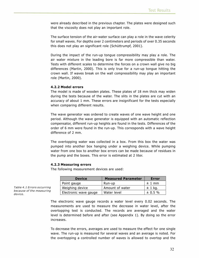
4.2.3 Measuring errors
The following measurement devices are used:
Device Measured Parameter Error
Point gauge Run-up ± 1 mm
Weighing device Amount of water ± 1 kg.
Electronic wave gauge Water level ± 0.5 %
Table 4.1 Errors occurring
because of the measuring
device.
The electronic wave gauge records a water level every 0.02 seconds. The
measurements are used to measure the decrease in water level, after the
overtopping test is conducted. The records are averaged and the water
level is determined before and after (see Appendix 1). By doing so the error
increases.
To decrease the errors, averages are used to measure the effect for one single
wave. The run-up is measured for several waves and an average is noted. For
the overtopping a controlled number of waves is allowed to overtop and the

33
Test Results
complete volume is measured. The combined measuring and model errors then
become as follow:
Parameter Error
Average run-up 3 mm.
Overtopping volume 3*10-3 m3/number of waves
Water level 0.5 mm
Table 4.2 Combined
measuring and test set-
up errors.
4.3 Quantitative Results
The reduction of the run-up is related to the energy dissipation. In chapter
2 the energy dissipation for flow around one object was mentioned. The
dimensionless numbers from chapter 2 and the flow profiles from chapter 3 are
used below to explain the results of the tests.
In chapter two dimensionless parameters are determined that affect the
dissipation of energy and the exchange of momentum during run-up with a
slender object:
∆Eg R z D
fg R z D R z
Dusmooth
usmooth usmooth
ρ ν⋅ ⋅ − ⋅=
⋅ − ⋅ −
( )
( ),( )
3
Equation 4.1
This is only true for one object. For a group of objects, like the plate with
the slits, the energy loss per unit length can be calculated by multiplying the
energy loss by the density, by n/l, in which n is the number of stems and l is
the hedge length. By doing so the interaction between the different objects is
neglected. The flow pattern around the objects interfere with each other and
this should be taken into account too. Full expression for the energy loss per
unit length then can be described as:
Equation 4.2
∆Eg R z D
l fg R z D R z
Dusmooth
usmooth usmooth
ρ ν⋅ ⋅ − ⋅=
⋅ − ⋅ −( )
/( )
,( )
,%3
⋅n
l
The energy loss per unit length is linked to the volume behind the run-up
hedge at the moment of maximum run-up. The energy of a run-up tongue can
for instance be calculated by calculating the potential energy of the run-up
tongue at the moment the maximum run-up height is reached. The reduction
of the run-up volume is determined by the same parameters as above:
Equation 4.3
∆VV
l fg R z D R z
D
n
l
usmooth usmooth/( )
,( )
,%=⋅ − ⋅ −
⋅
ν
34
Test Results
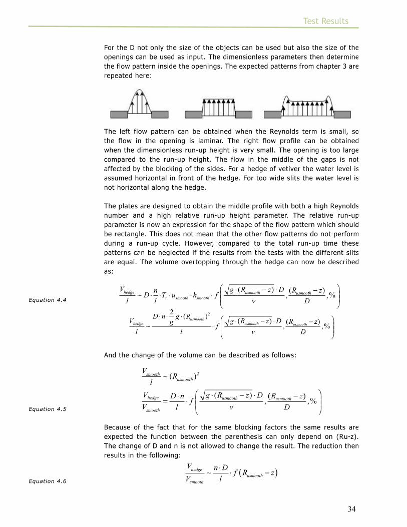
For the D not only the size of the objects can be used but also the size of the
openings can be used as input. The dimensionless parameters then determine
the flow pattern inside the openings. The expected patterns from chapter 3 are
repeated here:
The left flow pattern can be obtained when the Reynolds term is small, so
the flow in the opening is laminar. The right flow profile can be obtained
when the dimensionless run-up height is very small. The opening is too large
compared to the run-up height. The flow in the middle of the gaps is not
affected by the blocking of the sides. For a hedge of vetiver the water level is
assumed horizontal in front of the hedge. For too wide slits the water level is
not horizontal along the hedge.
The plates are designed to obtain the middle profile with both a high Reynolds
number and a high relative run-up height parameter. The relative run-up
parameter is now an expression for the shape of the flow pattern which should
be rectangle. This does not mean that the other flow patterns do not perform
during a run-up cycle. However, compared to the total run-up time these
patterns can be neglected if the results from the tests with the different slits
are equal. The volume overtopping through the hedge can now be described
as:
V
lDn
lT u h f
g R z D Rhedge
r smooth smooth
usmooth usmoo∼ ⋅ ⋅ ⋅ ⋅ ⋅
⋅ − ⋅( ),(
νtth z
D
−
),%
2
Equation 4.4
V
l
D ngg R
lf
g R z D
v
Rhedgeusmooth
usmooth usmooth∼
⋅ ⋅ ⋅⋅
⋅ − ⋅ −2 2( )
( ),( zz
D
),%
And the change of the volume can be described as follows:
V
lR
V
V
D n
lf
g R z D
v
smoothusmooth
hedge
smooth
usmooth
∼ ( )
( ),
2
=⋅
⋅⋅ − ⋅ (( )
,%R z
D
usmooth −
Equation 4.5
Because of the fact that for the same blocking factors the same results are
expected the function between the parenthesis can only depend on (R u-z).
The change of D and n is not allowed to change the result. The reduction then
results in the following:
V
V
n D
lf R z
hedge
smooth
usmooth∼
⋅⋅ −( )
Equation 4.6

35
Test Results
The problem with the dependency of (Ru-z) is that a dimension of length has
been introduced. The dimensions both on the left and right hand side of the
equations have to be the same. This can only be reached if:
f R z constant
V
VcD n
L
usmooth
hedge
smooth
−( ) =
= ⋅⋅Equation 4.7
So when a constant reduction is measured, the flow can be assumed to be
quasi-steady. And the forces are drag dominant. (see paragraph 3.1.2)
4.3.2 Overtopping
The amount of water passing through the hedge during one run-up cycle was
measured by collecting the water in a box. By doing so the amount of water
passing through the hedge is overestimated, because no water running down
the slope will reduce the run-up of the next wave. For overtopping on smooth
slopes the overtopping can be calculated by determining the imaginary run-up
tongue (Schüttrumpf, 2001).
Figure 4.5 Calculation of
the overtopping volumes
The run-up volume on the left side of the figure 4.5 needs to be measured.
Because of the overestimation the overtopping volumes found in tests with
a smooth slope, found a better fit with calculations which use the volume of
the run-up tongue above the crest level (right side of figure 4.5). (Battjes,
1976). The measured data were compared with calculations of the overtopping
volume, calculated by using ch= 0.284 and the measured run-up levels.

36
Test Results
Figure 4.6 Measured
overtopping volumes
versus the calculated
overtopping volumes.
The measured data are all larger than the calculated data, because of the
absence of a horizontal dike crest in the tests. The difference between the
calculated data and the measured data is about 20%. The calculation of the
overtopping itself gives an overestimation of 42%. So the total amount of
overestimation of the run-up tongue is 69 %. However, it is assumed that this
is the same for the overtopping with the hedges. The reduction in the volume of
overtopping can be seen in the graph below for the plates with 75% blocking.
Figure 4.7 Reduction of
the overtopping volume
with a blocking factor of
75%
The reduction of the overtopping volume is considerable. The volume is reduced
by over 55%. No significant differences could be found between the different
hedges with the different widths of the gaps except for the largest run-up. The
reduction is almost constant as expected.

37
Test Results
The tests were conducted with different breaker parameters. Because of that
the small differences can be explained. The influence of the breaker parameter
may be the effect of the reflection of the waves. On the other hand, it is more
likely that different breaker types create different amounts of turbulence in
the tip of the run-up tongue. In the formulas for the reduction of the run-up
the average velocities are used, which gives an underestimation of the forces.
Since the differences are small no further tests are conducted to measure the
influence of the breaker parameter.
Figure 4.8 Reduction of
the overtopping volumes
with a blocking factor of
60%
The reduction of the overtopping is much smaller than with the plate with 75
% blocking as can be expected. The reduction is about 40% as can be seen
from figure 4.8.
4.3.1 Run-up height
The run-up height and the run-up volume are strongly linked to each other.
Therefore run-up height should give the same trend as the run-up volume. The
results should be independent of the run-up height and only depend on the
blocking factor.

38
Test Results
For the hedges with a blocking factor of 75% the results are presented
below:
Figure 4.9 Reduction of
the run-up height with
75% blocking.
From this graph it can be seen that no differences significant are found in the
run-up height between the different slit width. On the other hand, no clear
trend can be observed. The reduction is over 25 % in all cases. In figure 4.10
the results from the hedge with the narrow slits are presented together with
some additional measurements. The reduction is now a function the breaker
parameter:
Figure 4.10 Reduction
of the run-up versus
breaker parameter.
The influence of the breaker parameter is visible in this graph. A higher
breaker parameter gives less reduction. A breaker parameter of 3 gives half
the reduction as the breaker parameter of 2.5. Only one point doesn’t fit, this
can be caused by the low Reynolds number because of the fact that this point
is measured at very low run-up.

39
Test Results
The reduction seems constant for different run-up heights if the breaker
parameter is kept constant. This means that the relative reduction of the run-
up height is independent of (Ru-z).
The breaker parameter determines the breaking of a wave. A surging wave with
a high breaker parameter has less turbulence at the tip of the run-up tongue
than plunging waves.
The reduction is determined by using an average velocity. In the case of higher
turbulent flow because of the differences in velocities are the forces on the
objects are larger. This increases the reduction of the run-up.
In figure 4.11 the results for the hedges with a blocking factor of 60% are
presented. Also no significant differences between the hedges, although the
widest slits tend to give less reduction in run-up.
Figure 4.11 Run-up
reduction with 60%
blocking.
In figure 4.12 the reduction again is set out versus the breaker parameter.
Figure 4.12 Run-up
reduction versus the
breaker parameter

40
Test Results
In this graph the same trend as with the hedges with a blocking factor of 75%
is visible. The relative reduction ΔRu/(Ru-z) seems independent of the run-up
height, but depends on the breaker parameter.
The differences between the two blocking factors are small especially for the
larger breaker parameter. The reduction of the run-up is for both blocking
factors about 20-25 % at a breaker parameter of 3.
4.3.3 Conclusion and Evaluation
The theory that the reduction is independent of the run-up height could not be
rejected. Both the relative reductions of the run-up height and the overtopping
volume were found constant over the run-up height. The run-up height
reduction by both hedges is at least 20% for the breaker parameters tested.
The reduction of the volumes is at least 55% for the 75% blocking hedge and
around 40% for the hedge with a blocking of 60%.
For the Reynolds numbers, the relative run-up height number and blocking
factors tested, the reduction of the run-up height through a plate with vertical
slits depends mainly on the breaker parameter. The differences in the results
for the different breaker parameters are larger than the differences between
the blocking factors tested. The run-up height is determined by the fast flowing
tip of the run-up tongue. For a Vetiver hedge with higher blocking factors at
the lower parts of the hedge the reduction of the run-up height could be more.
The reduction of the run-up height is difficult to use for further calculation
since the differences between the different breaker parameters are large.
The reduction of the overtopping volume is much more than the reduction of
the run-up height. The influence of the breaker parameter on the overtopping
volumes is very small.
Since the main reason to plant Vetiver on a dike is to decrease the overtopping
volumes, the reduction of volume is a better parameter to use for further
calculation than the reduction of the height.
Forces on the plates in the tests are drag dominant. This means that the flows
through the plates are quasi-steady. The forces on the plate are mainly caused
by the velocities and not by the acceleration or deceleration of the flow.
It is expected that for higher run-up heights the flow remains drag dominant.
(Ru-z)/D is only getting larger for higher run-up so the flow profile in the
opening remains a rectangle. For a real Vetiver hedge the D is getting smaller
this also causes (Ru-z)/D to increase so for a Vetiver hedge the flow is also drag
dominant. This is similar to the behavior with short waves through vegetation.

41
Test Results
A higher Keulegan-Carpenter parameter creates more drag dominant flow.
The hedges were designed to simulate the drag of Vetiver grass in steady flow.
Since the flow through the openings in the run-up tests were quasi-steady it
can be concluded that the plates with the slits are a good model for a Vetiver
hedge.

42
Vetiver on a Dike
5. VETIVER GRASS ON A DIKE
To determine the effect of Vetiver grass hedges on a dike an example is worked
out below. In this example a conventional dike with conventional armour
layer and a dike covered with Vetiver grass are designed and compared. The
differences in use of material and costs will are shown. In this example the
wave climate is determined by some rules of thumb, Therefore the examples
can only be used for comparison and indication.
5.1 Location
The location is in Vietnam in the coastal district southeast of Ho Chi Minh City.
This Can Gio district is a large biosphere reserve recognized by the UNESCO.
It covers 75,740 hectares and is dominated by mangroves both brackish and
salt water species. About 58,000 people are living within the boundaries of the
reserve of which 54,000 live in the transition area (1997). The district is the
poorest district of the Ho Chi Minh province. The biosphere reserve is expected
to be a site where eco-tourism and different sustainable economic activities
can be implemented to develop the area. (UNESCO, 2000). In the south of the
district there are some villages along the coast that need protection from the
waves coming from the sea.
Figure 5.1 Map of the Can
Gio district

43
Vetiver on a Dike
There is a large mud flat lying in front of the coast. This mud flat is protecting
the coast most of the time from wave attack. However during storms the water
level may rise because of wind set-up. The typhoon Linda (1997), one of the
severest typhoons of the century caused wind set-up of 1 meter at sea and 4
meters inside the delta. No levels of set-up along the coast are known. A set-up
of 2.5 meters along the coast seems a good assumption. From this maximum
water level the wave climate at the toe of the dike can be determined by the
following rule of thumb (d’Angremond, 2001):
H hs ≤ ⋅0 55.Equation 5.1
Breaking of the waves causes the wave spectrum to change; this is neglected
in this example. The spectral wave period is assumed to be 7 seconds, so the
value of the breaker parameter becomes 2.5.
5.2 Design of the Dike
The height of a dike is determined by the amount of overtopping allowed. In
the Netherlands the following design rule from van der Meer, 2001 is used to
determine the crest height:
q
g H
h
Hm
bk
m b f v⋅= ⋅ ⋅ ⋅ − ⋅ ⋅
⋅ ⋅ ⋅ ⋅
0
30
0 0
0 0674 3
1,
tanexp ,
αγ ξ
ξ γ γ γ γβ
With a maximum of
q
g H
h
Hm
k
m f⋅= ⋅ − ⋅ ⋅
⋅
0
30
0 2 2 31
, exp ,γ γ βEquation 5.2
In this equation q is the average discharge allowed the other factors are the
same as in equation 2.3. The discharge allowed is determined by the state
of the inner slope. In the guidelines the following average discharges are
mentioned:
0.1 l/m per s for sandy soil and a bad cover
1.0 l/m per s for clay with a reasonable well grass cover
10 l/m per s for a good grass cover or an armour layer.
The conventional dikes in the area consist of clay, covered with a geo-textile
and an armour layer of placed concrete blocks or placed granite stones on a
granular filter. This armour layer has a roughness of 0.95. The inner slope
is unprotected and just covered with some low grasses and weed. The outer
slope has a slope angle of 1:3. The inner slope is assumed 1:2.5. If an average
overtopping discharge of 0.1 l/m per second is used as a design rule, a dike
height of 4.57 meters will be necessary. The cross section of the dike is drawn
in figure 5.2.

44
Vetiver on a Dike
Figure 5.2 Cross-section
of the dike without
Vetiver grass.
Since a hedge of Vetiver grass will reduce the volume of overtopping by 55 %
the crest levels can be decreased. The new crest levels are given in the table
5.1:
Nr. of hedges q allowed without hedge hk above SWL
No hedge 0.1 4.58
1 hedge 0.22 4.12
2 hedges 0.49 3.67
3 hedges 1.1 3.21
Table 5.1 Crest heights
for different numbers
of hedges on the outer
slope
The reduction by multiple hedges is calculated by multiplying the reduction
of one hedge. In reality some water will remain between the hedges and the
reduction is even more.
The number of hedges to be planted on a slope is limited by the length of
the slope and the strength of the hedges. The hedges need to be planted
with a spacing of one meter. This allows people to move through the hedges
for maintenance and inspection. Near the still water line the hedges will be
overloaded and water will flow over the hedges. Water flowing over the hedges
is a different mechanism from water flowing through the hedges.
In chapter 2 it can be found that there is limited knowledge of the strength of
mature hedges in flow. The failure mechanism is unknown. For one stem Dunn,
1996 states that after overloading of a stem, the stem will break or develop a
hinge point. For a hedge the following extreme failure mechanisms are possible
or a combination of those:
• Breaking or hinging of several weaker stems at low heights. A more open
hedge remains that can cope with the extra discharge through the hedge.
• Breaking or hinging of all stems at a certain height. The lower part can cope
with the load and when overloaded the extra flow will simply flow over the
hedge.
• Brending through an elastic range so after overloading the hedge turns
back in its original state.

45
Vetiver on a Dike
In further calculations the height of 0.4 m is considered as the height, where
the stems will break or develop a hinge point or bend. This height can be
exceeded by some of the run-up layers, but most of the water overtopping the
dike needs to flow through the hedges. Other wise the proposed reduction is not
feasible. In figure 5.3 a probability distribution function for wave overtopping
is shown:
Figure 5.3 probability
distribution function
for wave overtopping
volumes per wave;
q = 1 l/s per m width, Tm
= 5 s and Pov = 0.10 van
der Meer (2002)
Waves with a high probability overtop the dike often but the damage caused is
small. Larger waves cause more damage, however their occurrence is very low.
Vetiver grass should be able to withstand the most damaging waves.
In this case the 1% wave run-up height is assumed as a design run-up height.
For determining the Ru1%
van Gent (2002) is used:
R
Hc for p
R
Hc
cfor p
c
u
s
u
s
10 0
11
2
0
2 0 2
%
%
( )
( )
.
γξ ξ
γ ξξ
⋅= ⋅ ≤
⋅= − ≥
=
0
0
55
1 45 5 1
1
2
0
0
1
⋅ = ⋅
= =
c
c
for Ru
ξ p 0.5c
c
c c
1
0
0 1% . .Equation 5.3
In this case the average Ru1%
is 4.31 meters. The layer thickness of the run-
up tongue can be calculated for a smooth slope by the equation proposed by
Schüttrumpf, 2001:
h R zu= ⋅ −0 284. ( )Equation 5.4
This is perpendicular to the slope for perpendicular to the hedge ch should be
0.3. If two hedges are planted the lower hedge is planted 33 cm lower than the
crest. The higher hedge is planted on the top of the slope. The lower hedge is
planted at 3.37 m from the still water line. In this case the layer thickness is
0.28 m for a Ru1%
. This is well below the 0.4 m height of the hedge. However,
the 0.28 m is calculated for smooth slopes and reflection of part of the wave is

46
Vetiver on a Dike
not taken into account. So a small part of the water will splash over the hedge
, this is considered negligible.
If the height of the hinge or bending point is taken at 0.6 m a third hedge
may be considered. A third hedge would need to be planted 0.66 meter below
the crest level. At this level the water layer thickness is about 0.53 m for Ru1%
.
Again this is only for a smooth slope and probably a lot of water is flowing over
the hedge and the reduction of 55% is not feasible. So, if only water flowing
through the hedge is considered, 2 hedges is probably the maximum number
of hedges needed
If water is flowing over the hedges, the hedges can be interpreted as artificial
roughness elements. Planting more hedges below the 2 already planted, will
also have effect on the run-up. This is not tested however, in van der Meer,
2002 roughness elements are described. The hedges can be described as
ridges. For small ridges a roughness factor of 0.75 is found. For a cover with
small grass, that is sod forming, the roughness is 1,0. Since the roughness is
not investigated a safe roughness factor of 0.95 is used for overloaded Vetiver
grass the same as for the placed blocks. The new dike can be seen in the
picture below:
Figure 5.4 Cross section
of a dike with Vetiver
grass
When an average overtopping discharge of 1 liter/m per second is allowed,
considerably more water is flowing over the dike. Allowing more water to
overtop the dike can only be done if a good inner slope is present. A good inner
slope can be very expensive in construction or management. The heights of a
conventional dike and a dike with hedges is described below:
Nr. of hedges q allowed without hedge hk above SWL
No hedge 1 3.26
1 hedge 2.2 2.81
2 hedges 4.9 2.36
Table 5.2 Crest heights
for different numbers
of hedges on the outer
slope
The Ru1%
is 4.31 meters and water will flow over the hedges, since the layer
thickness will be 0.45 meters at the top of the slope. This is a small amount from
the total number of waves spilling over the crest of the dike. Over 10% of the
waves will overtop this dike since Ru10%
is 3.31 m. However, the 1% wave does

47
Vetiver on a Dike
considerable more damage. So for a well managed inner slope the reduction of
the run-up by flowing through a Vetiver hedge is small. If the Vetiver hedges
can be considered as artificial roughness elements the construction costs can
still be decreased. The dike with Vetiver as is drawn below:
Figure 5.5 Cross section
of a dike with Vetiver
grass (q= 1.0 l/m/s)
From the calculations above it can be concluded that the effect of Vetiver
hedges can be considerable if the average discharge over the dike is small.
If the inner slope is protected with a good armour layer planting of Vetiver
hedges on the outer slope is not very useful.
5.5 Construction Costs
For the construction costs the following specific costs were applied.
Material Unit Price
Clay m3 $ 5
Vetiver hedge m $ 4
Armour layer m3 $ 12Table 5.3 Prices of
different materials
The thickness of the armour layer is assumed to be 0.4 m. The construction
costs of the different dikes are described below:
Dike Price/m
Conventional dike q = 0.1 l/m/sec. $ 871
Vetiver dike q= 0.1 l/m/sec. $ 691
Conventional dike q = 1.0 l/m/sec. $ 603
Vetiver dike q = 1.0 l/m/sec $ 588Table 5.4 Costs of the
different dikes
In this calculation the extra measures for allowing 1.0 l/m/s over the dike are
not taken into account. This might be very expensive and the lower dike may
eventually cost more than the dike with an allowed overtopping of 0.1 l/m/
s. The results of the conventional dike and the Vetiver dike with the higher
overtopping can be compared because, both might need the measures for
protection of the inner slope.

48
Vetiver on a Dike
5.4 Management Considerations
The height where the stems will break or develop a hinge point is very
important in these calculations. The height may be change due to management
techniques. By pruning the Vetiver hedge at 0.4 m height the old stems may
enforce the lower part and stimulate breaking or hinging at a height of 0.4 m.
Since maintenance and inspection will be needed, paths have to be cut through
the hedges. These will become week spots in the dike armour layer. These
paths and the inner slope behind it need extra protection.
In between the hedges the slope should be protected with small good sod
forming grass. Regular pruning of Vetiver grass, so sunlight can break through,
might help growing the grass in between the hedges.
Because of all these management measures, the management of Vetiver grass
hedges can be more expensive than the management of a conventional armour
layer. However in countries with low wages like Vietnam and Bangladesh the
reduction of the construction costs will be considerably more than the extra
management costs
5.5 Conclusions
The reduction of the costs can be 20% as the example above shows. However,
the result highly depends on the average discharge allowed. For low average
discharges Vetiver can be very effective. The calculations above show that
some assumptions have to be made before the effect could be calculated. In
further research the following could be investigated:
• Roughness when the run-up tongue flows over the Vetiver hedge.
• Failure mechanism and the maximum load.

.
50
Conclusions and Recommendations
6 CONCLUSIONS AND RECOMMENDATIONS
In the first chapter a problem definition was described. From that the objective of
this research was derived. The objective of this research is repeated below:
“Determine the effect of Vetiver grass hedges on wave run-up”
A relationship has to be found between the wave height, hedge characteristics
and run-up level. The following questions related to this objective will need to
be answered:
• What is the hydraulic resistance of Vetiver grass hedges
• What is the effect of different planting configurations on the reduction of
the wave run-up?
In this chapter the results are compared to the objective stated. The conclusions
are followed by recommendations for further research.
6.1 Conclusions
Tests show that a plate with slits can represent a hedge of Vetiver grass in run-
up. A plate with slits and a blocking factor of 75% has about the same drag
factor as a Vetiver grass hedge. .
The theory that the reduction of run-up only depends on the blocking factor
could not be rejected. Small scale run-up tests show that a plate with 75%
gives a reduction of at least 55% of the overtopping volumes. The run-up
height is reduced by more than 20%.
A more open hedge with a blocking factor of 60% blocking reduces the
overtopping volume by 40%. The run-up height is also reduced by more than
20%.
The reduction of the run-up height depends amongst others on the breaker
parameter. Since the overtopping volume is less dependent on the breaker
parameter, this should be used for further calculation.
For dikes with a low average overtopping discharge allowed (0.1 l/m/ second),
two hedges placed on the top of the slope have the most effect. It can reduce
the height of the dike by about 0.9 m. With an average discharge of over 1
l/m/s the effect of a Vetiver hedge is considerably less.
6.2 Recommendations
In some calculations in this report assumptions have been made. These
assumptions have to be verified. This report can be the part of a larger research

51
Conclusions and Recommendations
on Vetiver grass. A possible lay-out of this research can be seen below:
Table 5.4 Possible lay-
out of the research on
Vetiver grass
The research in this report is part of phase one and two. Phase two is not
finished and can be extended by the following research:
• Assumptions about the failure mechanisms in chapter 5 are very crucial for
the reduction of the costs. The failure of Vetiver hedges can be tested in
flumes where the forces on Vetiver during wave run-up are simulated by a
hydraulic jump. Layer thickness celerity and bore wedge angle need to be
the same as with run-up.
• The roughness factor of Vetiver grass hedges when overloaded was assumed
to be 0.95. It is very well possible that the reduction may be even larger.
This needs to be tested.
For Phase three the following can be said:
• Scaling of the hedges is good possible. Large scale tests in laboratory flumes
tend to be very expensive. However, they need to be done to get statistical
prove of the reduction of a Vetiver hedge in run-up. This is necessary
because design rules have to be created and should contain statistical
prove.
Phase four can also be started:
• It is yet not possible to use Vetiver grass in design rules because of the
reason stated above. Planting Vetiver on a dike for different testing purposes
can be done, however without relying on it. If no other options are possible
to strengthen a dike Vetiver grass can yet be a last option.
Next to more research on Vetiver grass in the run-up zone other investigation
should also be started. Research on the use of Vetiver grass for reinforcement
of the inner slope of a dike. This would allow more overtopping and would also
lower the dike. If good results with Vetiver on the inner slope are acquired the
use of Vetiver on the outer slope could be abandoned.

52
References
REFERENCES
Battjes, J.A., Roos A., 1976, Characteristics of flow in run-up of
periodic waves, Communications on Hydraulics Department of Civil
Engineering Delft University of Technology. Report no. 75-3
Ben Chie Yen, January 2002, Open Channel Flow Resistance, Journal
of Hydraulic engineering. 20-39
Dabney, S.M. et al. 1996 Stiff-Grass Hedges a vegetative Alternative
for Sediment Control, Proceedings of the Sixth Federal Interagency
Sedimentation Conference X 62-69
Dabney, S.M., 2003, Erosion Control, Vegetative from Encyclopedia of
Water Science, Marcel Dekker, inc.
Dabney, S.M., Shields, Jr. F.D., Temple, D.M., Langendoen, E.J., 2004.
Erosion Processes in Gullies Modified by Establishing Grass Hedges.
Transactions of the ASAE 47(5) 1561-1571
Dalton, P. A., Smith, R.J., Truong, P.N.V.,1996. Vetiver grass hedges for
erosion control on a cropped floodplain: hedge hydraulics. Agricultural
Water Management 31 91-104
d’Angremond, K, van Roode, K.C. 2001, Breakwaters and closure
dams. Delft University Press
Dunn, G.H and Dabney, S.M., 1996. Modulus of Elasticity and Moment
of Inertia of Grass Hedge Stems. Transactions of the ASAE 39(9) 947-
952
Kindsvater, C.E., Carter, R.W., Tracy, H.J., 1953. Computation of Peak
Discharge at Contractions, Geological Survey Circular 284
Maaskant, I., 2005 Toepassingsmogelijkheden van Vetiver gras en
Cyperus Rotundus op dijken. Msc-thesis Delft University of Technology,
Faculty of Civil Engineering, Department of Hydraulic Engineering
Metcalfe, O. Truong, P., Smith, R. 2003. Hydraulic Characteristics of
Vetiver Hedges in Deep Flows. Proceedings of the Third International
Vetiver Conference.
Meyer, L.D., Dabney, S.M., Harmon, W.C., 1995. Sediment-trapping
Effectiveness of Stiff-grass Hedges. Transactions of the ASAE 38(3)
809-815

53
References
Schüttrumpf, H. 2001, Wellenuberlaufstromung bei Seedeichen.
Leichtweiss-Institut fur Wasserbau Mitteilungen Heft 149 1-128
Schuttrumpf, H., van Gent, M.R.A. 2003, Wave overtopping at seadikes,
Coastal Structures 2003.
Temple, D.M., Dabney, S.M., 2001, Hydraulic Performance Testing of
stiff Grass Hedges. Proceedings of the Seventh Federal Interagency
Sedimentation Conference XI 118-124
van Gent, M.R.A. 2002. Wave overtopping events at Dikes, Proceedings
of the ICCE 2002.
van der Meer, J.W. 2002, Technisch rapport Golfoploop en Golfoverslag
bij Dijken. Technisch Adviescommissie Waterkeringen
Appendix I
I
APPENDIX 1 PROCESSING OF THE MEASUREMENTS
The results presented in chapter 4 are derived from the measurements as
described in this appendix. The processing is done for every test. In this
appendix example B6 is used which means the hedge named B and wave climate
6 (see chapter 3). The measurements are described below:
Measured Value
Water level measurement (h) 50 mm
Measured run-up height with hedge (Ru) 378 mm
Measured run-up height smooth slope 427 mm
Height hedge at the crest side (z) 258 mm
Table I.I Measured values
during run-up tests.
Quantity Value
(Ru-z) 120 mm
(Rusmooth
- z) 169 mm
Reduction (Rusmooth
- Ru)/(Rusmooth
- z) 0.29Table I.II Calculated
quantities
After the values are known the error-margins are calculated in the table below.
The values for the measurement errors are determined in chapter 4.
Error margin Value
(Ru-z)max
120+3 mm 123 mm
(Ru-z)min
120-3 mm 117 mm
(Rusmooth
-z) max
169+3 mm 172 mm
(Rusmooth
-z) min
169-3 mm 166 mm
Reduction max (172-117)/172 0.32
Reduction min (166-123)/166 0.26Table I.III Determining
the error margins for the
run-up tests
For the calculation of the overtopping the following procedure is used:
Measured Value
Overtopping Volume 136 liters
Number of waves 30
Average volume 4.53 liters
Volume per meter width (V*1/0.8) 5662 mm2
Table I.IV Measurements
and calculated quantities
of the overtopping test
The water level is recorded with the wave gauge. The recorded values are
shown in the graph below. On the right the water level is averaged over the
wave period.

Appendix I
II
Figure I.I The output of
the wave gauge. The
negative waterlevel is
because of the conversion
to the same levels of the
point gauge.
Measured Value
hstart
52.3 mm.
hend
46.6 mm.Table I.V Start and end
value of the waterlevel
The overtopping volume is a function of (Ru-z)2. Therefore not the average water
level was taken as reference level, but the water level at 1/3 of the difference.
This is the water level at which the average run-up volume measured is taking
place. From this reference water level the volume has to be calculated to 50
mm.
Quantity Value
Hreference
50.4 mm.
Waterlevel difference -0.44 mm.Table I.VI Determining
the reference waterlevel
Quantity Value
(Ru-z) 120 mm
Sqrt(10) * (Ru-z) * Δh -162 mm2
Overtopping volume at h=50 mm 5504 mm2
Table I.VII Table with the
conversion of the average
volume to the volume at
h = 50 mm.
The same is done for the overtopping for with the smooth slope. The overtopping
for the smooth slope is 16403 mm2. Now the error margins can be established
the errors are described in chapter 4 and repeated below:
Parameter Error
Average run-up 3 mm
Overtopping volume 3*10-3 m3/number of waves
Water level 0.5 mTable I.IIX Table with the
measurement errors
Now the maximum and minimum values can be calculated:

Appendix I
III
Quantity Value
Overtopping Volumemin
133 liters
Number of waves 30
Average volumemin
4.43 liters
hstart max
52.8 mm.
hend max
47.1 mm.
Hreference max
50.9 mm.
Waterlevel difference -0.94 mm.
Volume per meter width (V*1/0.8) 5541 mm2
(Ru-z) 123 mm
Sqrt(10) * (Ru-z) * Δh -350.5 mm2
Overtopping volume at h=50 mm 5195 mm2
Table I.IX Determining
the minimum overtopping
volume
Quantity Value
Overtopping Volumemin
139 liters
Number of waves 30
Average volumemin
4.63 liters
hstart max
51.8 mm.
hend max
46.1 mm.
Hreference max
49.5 mm.
Waterlevel difference +0.54 mm.
Volume per meter width (V*1/0.8) 5791 mm2
(Ru-z) 117 mm
Sqrt(10) * (Ru-z) * Δh +19 mm2
Overtopping volume at h=50 mm 5811 mm2
Table I.X Determining the
maximum overtopping
volume
The same procedure is used to calculate the values for a smooth slope
Parameter Value
V 16403 mm2
Vmax
16749 mm2
Vmin
16055 mm2
Table I.XI Overtopping
values for the smooth
slope
The maximum and minimum reduction are calculated below:
Parameter Value
Reduction (16403-5504)/16403 0.66
Reductionmax
(16749-5195)/16749 0.69
Reductionmin
(16055-5811)/16055 0.64
Table I.XII Reduction of
the overtopping and the
error margins.