runge-kuttadiscontinuous galerkinmethod witha …zhongxh/paper/hweno.pdfthe runge-kutta...

Runge-Kutta discontinuous Galerkin method with a

simple and compact Hermite WENO limiter

Jun Zhu1, Xinghui Zhong2, Chi-Wang Shu3 and Jianxian Qiu4,∗

1 College of Science, Nanjing University of Aeronautics and Astronautics, Nanjing,Jiangsu 210016, P.R. China.2 Department of Mathematics, Michigan State University, East Lansing, MI 48824,USA.3 Division of Applied Mathematics, Brown University, Providence, RI 02912, USA.4 School of Mathematical Sciences and Fujian Provincial Key Laboratory of Math-ematical Modeling and High-Performance Scientific Computation, Xiamen Univer-sity, Xiamen, Fujian 361005, P.R. China.

Abstract. In this paper, we propose a new type of weighted essentially non-oscillatory(WENO) limiter, which belongs to the class of Hermite WENO (HWENO) limiters, forthe Runge-Kutta discontinuous Galerkin (RKDG) methods solving hyperbolic conser-vation laws. This new HWENO limiter is a modification of the simple WENO limiterproposed recently by Zhong and Shu [29]. Both limiters use information of the DGsolutions only from the target cell and its immediate neighboring cells, thus maintain-ing the original compactness of the DG scheme. The goal of both limiters is to obtainhigh order accuracy and non-oscillatory properties simultaneously. The main noveltyof the new HWENO limiter in this paper is to reconstruct the polynomial on the targetcell in a least square fashion [8] while the simple WENO limiter [29] is to use the entirepolynomial of the original DG solutions in the neighboring cells with an addition ofa constant for conservation. The modification in this paper improves the robustnessin the computation of problems with strong shocks or contact discontinuities, withoutchanging the compact stencil of the DG scheme. Numerical results for both one andtwo dimensional equations including Euler equations of compressible gas dynamicsare provided to illustrate the viability of this modified limiter.

AMS subject classifications: 65M60, 35L65

Key words: Runge-Kutta discontinuous Galerkin method; HWENO limiter; conservation law.

∗Corresponding author. Email addresses: [email protected] (J. Zhu), [email protected] (X. Zhong),[email protected] (C.-W. Shu), [email protected] (J. Qiu)

http://www.global-sci.com/ Global Science Preprint

2

1 Introduction

In this paper, we are interested in solving the hyperbolic conservation law{

ut+ f (u)x =0,u(x,0)=u0(x),

(1.1)

and its two-dimensional version{

ut+ f (u)x+g(u)y=0,u(x,y,0)=u0(x,y),

(1.2)

using the Runge-Kutta discontinuous Galerkin (RKDG) methods [4–7], where u, f (u)and g(u) can be either scalars or vectors.

It is not an easy task to solve (1.1) and (1.2) since solutions may contain discontinu-ities even if the initial conditions are smooth. Discontinuous Galerkin (DG) methods cancapture weak shocks and other discontinuities without further modification. However,for problems with strong discontinuous solutions, the numerical solution has significantoscillations near discontinuities, especially for high order methods. A common strategyto control these spurious oscillations is to apply a nonlinear limiter. One type of limitersis based on the slope methodology, such as the minmod type limiters [4–7], the momentbased limiter [2] and an improved moment limiter [3]. These limiters do control theoscillations well, however they may degrade accuracy when mistakenly used in smoothregions of the solution. Another type of limiters is based on the weighted essentially non-oscillatory (WENO) methodology [11–13,17], which can achieve both high order accuracyand non-oscillatory properties. The WENO limiters introduced in [18–20, 22, 30] and theHermite WENO limiters in [19,22] belong to this type. These limiters are designed basedon the WENO finite volume methodology which require a wider stencil for higher orderschemes. Therefore, it is difficult to implement them for multi-dimensional problems,especially on unstructured meshes. An alternative family of DG limiters which servesat the same time as a new PDE-based limiter, as well as a troubled cells indicator, wasintroduced by Dumbser et al. [10].

More recently, a particularly simple and compact WENO limiter, which utilizes fullythe advantage of DG schemes in that a complete polynomial is available in each cellwithout the need of reconstruction, is designed for RKDG schemes in [29]. The two ma-jor advantages of this simple WENO limiter are the compactness of its stencil, whichcontains only immediate neighboring cells, and the simplicity in implementation, espe-cially for unstructured meshes [31]. However, it was observed in [29] that the limitermight not be robust enough for problems containing very strong shocks or low pres-sure problem, especially for higher order polynomials, for example the blast wave prob-lems [23,28] and the double rarefaction wave problem [16], making it necessary to applyadditional positivity-preserving limiters [27] in such situation. In order to overcome thisdifficulty, without compromising the advantages of compact stencil and simplicity of lin-ear weights, we present a modification of the limiter in the step of preprocessing the

3

polynomials in the immediate neighboring cells before applying the WENO reconstruc-tion procedure. This preprocessing is necessary to maintain strict conservation, and is de-signed in [29] to be a simple addition of a constant to make the cell average of the prepro-cessed neighboring cell polynomial in the target cell matching the original cell average.In this paper, a more involved least square process [8] is used in this step. The objective isto achieve strict conservation while maintaining more information of the original neigh-boring cell polynomial before applying the WENO procedure. Numerical experimentsindicate that this modification does improve the robustness of the limiter.

This paper is organized as follows: In Section 2, we provide a brief review of RKDGfor one dimensional and two dimensional cases. In Section 3, we provide the details ofthe new HWENO limiter for one dimensional scalar and system cases. In Section 4, weprovide the details of the HWENO limiter for two dimensional scalar and system cases.We demonstrate the performance of our HWENO limiter with one and two dimensionalnumerical examples including Euler equations of compressible gas dynamics in Section5. Concluding remarks are given in Section 6.

2 Review of RKDG methods

In this subsection, we give a brief review of the RKDG methods for solving one and twodimensional conservation laws.

One dimensional case. Given a partition of the computational domain consistingof cells Ij = [xj− 1

2,xj+ 1

2], j= 1,··· ,N, denote the cell center by xj =

12(xj− 1

2+xj+ 1

2), and the

cell size by ∆xj = xj+ 12−xj− 1

2. The DG method has its solution as well as the test function

space given by Vkh ={v(x):v(x)|Ij

∈Pk(Ij)}, where P

k(Ij) denotes the set of polynomials ofdegree at most k defined on Ij. The semi-discrete DG method for solving (1.1) is defined

as follows: find the unique function uh(·,t)∈Vkh such that for j=1,··· ,N,

∫

Ij

(uh)tvdx−∫

Ij

f (uh)vx dx+ f j+ 12v(x−

j+ 12

)− f j− 12v(x+

j− 12

)=0 (2.1)

holds for all test functions v∈Vkh , where u±

j+ 12

=uh(x±j+ 1

2

,t) are the left and right limits of

the discontinuous solution uh at the interface xj+ 12

and f j+ 12= f (u−

j+ 12

,u+j+ 1

2

) is a monotone

flux for the scalar case and an exact or approximate Riemann solver for the system case.

Two dimensional case. Given a partition of the computational domain consistingof rectangular mesh consisting of cells Iij = [xi− 1

2,xi+ 1

2]×[yj− 1

2,yj+ 1

2], for i= 1,··· ,Nx and

j=1,··· ,Ny with the cell sizes xi+ 12−xi− 1

2=∆xi, yj+ 1

2−yj− 1

2=∆yj and cell centers (xi,yj)=

( 12(xi+ 1

2+xi− 1

2), 1

2(yj+ 12+yj− 1

2)). We now give the new test function space Wk

h ={p : p|Iij∈

Pk(Iij)} as the polynomial spaces of degree of at most k on the cell Iij. The semi-discrete

DG method for solving (1.2) is defined as follows: find the unique function u∈Wkh such

4

that, for all 1≤ i≤Nx and 1≤ j≤Ny,

∫

Ii,j

(uh)tvdxdy=

∫

Ii,j

f (uh)vx dxdy−∫

Ij

fi+ 12(y)v(x−

i+ 12

,y)dy+∫

Ij

fi− 12(y)v(x+

i− 12

,y)dy

+∫

Ii,j

g(uh)vy dxdy−∫

Ii

gj+ 12(x)v(x,y−

j+ 12

)dx+∫

Ii

gi− 12(x)v(x,y+

j− 12

)dx,

(2.2)

hold for all the test function v∈Wkh , where the “hat” terms are again numerical fluxes.

The semi-discrete schemes (2.1) and (2.2) can be written as

ut= L(u)

where L(u) is the spatial discretization operator. They can be discretized in time by anon-linearly stable Runge-Kutta time discretization [25], e.g. the third-order version:

u(1) = un+∆tL(un),

u(2) =3

4un+

1

4u(1)+

1

4∆tL(u(1)), (2.3)

un+1 =1

3un+

2

3u(2)+

2

3∆tL(u(2)).

As in [29], to apply a nonlinear limiter for the RKDG methods, for simplicity, we takethe forward Euler time discretization of the semi-discrete scheme (2.1) as an example.Starting from a solution un

h ∈ Vkh at time level n (u0

h is taken as the L2 projection of the

analytical initial condition into Vkh ). We would like to “limit” it to obtain a new function

un,new before advancing it to next time level. That is: find un+1h ∈Vk

h , such that, for j =1,··· ,N,

∫

Ij

un+1h −un,new

h

∆tvdx−

∫

Ij

f (un,newh )vx dx+ f n,new

j+ 12

v(x−j+ 1

2

)− f n,new

j− 12

v(x+j− 1

2

)=0 (2.4)

holds for all test functions v∈Vkh . The limiting procedure to go from un

h to un,newh will be

discussed in the following sections.

3 New HWENO limiter in one dimension

In this section, we describe the details of the modified HWENO reconstruction procedureas a limiter for the RKDG method in the one dimensional scalar and system cases.

5

3.1 The troubled cell indicator in one dimension

An important component of the simple WENO limiter in [29] is the identification of trou-bled cells, which are cells that may contain discontinuities and in which the WENO lim-iter is applied. We will use the KXRCF shock detection technique developed in [15] todetect troubled cells. We divide the boundary of the target cell Ij into two parts: ∂I−j and

∂I+j , where the flow is into (v·n < 0, n is the normal vector to ∂Ij and v is the velocity)

and out of (v·n> 0) Ij, respectively. Here, we define v, taking its value from inside thecell Ij as f ′(u) and take u as the indicator variable for the scalar case. The target cell Ij isidentified as a troubled cell when

|∫

∂I−j(uh(x,t)|Ij

−uh(x,t)|Il)ds|

∆xk+1

2j |∂I−j |·||uh(x,t)|Ij

||>Ck, (3.1)

where Ck is a constant, usually, we take Ck = 1 as in [15]. Here Il, for l = j−1 or j+1, denotes the neighboring cell sharing the end point ∂I−j with Ij. uh is the numerical

solution corresponding to the indicator variable(s) and ||uh(x,t)|Ij|| is the standard L2

norm in the cell Ij.

3.2 HWENO limiting procedure in one dimension: scalar case

In this subsection, we present the details of the HWENO limiting procedure for the scalarcase. The idea of this new HWENO limiter is to reconstruct a new polynomial on thetroubled cell Ij which is a convex combination of three polynomials: the DG solutionpolynomial on this cell and the “modified” DG solution polynomials on its two imme-diate neighboring cells. The modification procedure is in a least square fashion [8]. Theconstruction of the nonlinear weights in the convex combination coefficients follows theclassical WENO procedure.

Assume Ij is a troubled cell.Step 1.1. Denote the DG solution polynomials of uh on Ij−1, Ij+1, Ij as polynomials

p0(x), p1(x) and p2(x), respectively. Now we want to find the modified version of p0(x),denoted as p0(x) on the cell Ij−1 in a least square fashion [8]. The modification procedureis defined as follows: p0(x) is the solution of the minimization problem

min∀φ(x)∈Pk(Ij−1)

{

∫

Ij−1

(φ(x)−p0(x))2dx

}

, (3.2)

subject to ¯φ= ¯p2, where

¯φ=1

∆xj

∫

Ij

φ(x)dx, ¯p2 =1

∆xj

∫

Ij

p2(x)dx.

Here and below ¯⋆ denotes the cell average of the function ⋆ on the target cell.

6

Similarly, p1(x) is the solution of the minimization problem

min∀φ(x)∈Pk(Ij+1)

{

∫

Ij+1

(φ(x)−p1(x))2dx

}

(3.3)

subject to ¯φ= ¯p2.For notational consistency we denote p2(x)= p2(x).The final nonlinear HWENO reconstruction polynomial pnew

2 (x) is now defined by aconvex combination of these modified polynomials:

pnew2 (x)=ω0 p0(x)+ω1 p1(x)+ω2 p2(x). (3.4)

According to the modification procedure, it is easy to prove that pnew2 has the same cell

average and order of accuracy as p2 if the weights satisfy ω0+ω1+ω2 = 1. The convexcombination coefficients ωl,l=0,1,2 follow the classical WENO procedure [1, 12, 13]. Wediscuss it in the following steps.

Step 1.2. We choose the linear weights denoted by γ0,γ1,γ2. As in [29], we haveused complete information of the three polynomials p0(x), p1(x), p2(x) in the three cellsIj−1, Ij+1, Ij, hence we do not have extra requirements on the linear weights in order tomaintain the original high order accuracy. The linear weights can be chosen to be anyset of positive numbers adding up to one. The choice of these linear weights is thensolely based on the consideration of a balance between accuracy and ability to achieveessentially nonoscillatory shock transitions. In all of our numerical tests, following thepractice in [9, 29], we take γ2=0.998 and γ0=γ1=0.001.

Step 1.3. We compute the smoothness indicators, denoted by βℓ, ℓ= 0,1,2, whichmeasure how smooth the functions pℓ(x), ℓ=0,1,2, are on the target cell Ij. The smallerthese smoothness indicators are, the smoother the functions are on the target cell. We usethe similar recipe for the smoothness indicators as in [13]:

βℓ=k

∑l=1

∆x2l−1j

∫

Ij

(

1

l!

dl

dxlpℓ(x)

)2

dx, ℓ=0,1,2. (3.5)

Step 1.4. We compute the non-linear weights based on the smoothness indicators:

ωi=ωi

∑2ℓ=0ωℓ

, ωℓ=γℓ

(ε+βℓ)2. (3.6)

Here ε is a small positive number to avoid the denominator to become zero. We takeε=10−6 in our computation.

Step 1.5. The final nonlinear HWENO reconstruction polynomial is given by (3.4), i.e.unew

h |Ij= pnew

2 (x)=ω0 p0(x)+ω1 p1(x)+ω2 p2(x).It is easy to verify that pnew

2 (x) has the same cell average and order of accuracy as theoriginal one p2(x), on the condition that ∑

2ℓ=0ωℓ=1.

7

3.3 HWENO limiting procedure in one dimension: system case

In this subsection, we present the details of the HWENO limiting procedure for one di-mensional systems.

Consider equation (1.1) where u and f (u) are vectors with m components. In order toachieve better non-oscillatory qualities, the HWENO reconstruction limiter is used witha local characteristic field decomposition. In this paper, we consider the following Eulersystem with m=3.

∂

∂t

ρρµE

+∂

∂x

ρµρµ2+p

µ(E+p)

=0, (3.7)

where ρ is the density, µ is the x-direction velocity, E is the total energy, p is the pressureand γ=1.4 in our test cases. We denote the Jacobian matrix as f ′(u), where u=(ρ,ρµ,E)T .We then give the left and right eigenvector matrices of such Jacobian matrix as:

Lj(u)=

B2+µ/c

2−

B1µ+1/c

2

B1

2

1−B2 B1µ −B1

B2−µ/c

2−

B1µ−1/c

2

B1

2

, (3.8)

and

Rj(u)=

1 1 1µ−c µ µ+c

H−cµ µ2/2 H+cµ

, (3.9)

where c=√

γp/ρ, B1=(γ−1)/c2, B2=B1µ2/2 and H=(E+p)/ρ.Assume the troubled cell Ij is detected by the KXRCF technique [15] by using (3.1),

where v=µ is the velocity and again v takes its value from inside the cell Ij. We take boththe density ρ and the total energy E as the indicator variables. Denote p0, p1, p2 to be theDG polynomial vectors, corresponding to Ij’s two immediate neighbors and itself. Thenwe perform the characteristic-wise HWENO limiting procedure as follows:

Step 2.1 Compute Lj = Lj(uj) and Rj =Rj(uj) as defined in (3.8) and (3.9), where uj isthe cell average of u on the cell Ij.

Step 2.2. Project the polynomial vectors p0, p1, p2 into the characteristic fields ˜pℓ =Lj pℓ, ℓ= 0,1,2, each of them being a 3-component vector and each component of thevector is a k-th degree polynomial.

Step 2.3. Perform Step 1.1 to Step 1.5 of the HWENO limiting procedure that has beenspecified for the scalar case, to obtain a new 3-component vector on the troubled cell Ij as˜pnew

2 .Step 2..4. Project ˜pnew

2 back into the physical space to get the reconstruction polyno-mial, i.e. unew

h |Ij=Rj ˜pnew

2 .

8

4 New HWENO limiter in two dimension

4.1 The troubled cell indicator in two dimension

We use the KXRCF shock detection technique developed in [15] to detect troubled cellsin two dimensions. We divide the boundary of the target cell Iij into two parts: ∂I−ij and

∂I+ij , where the flow is into (v·n < 0, n is the normal vector to ∂Iij) and out of (v·n > 0)

Iij, respectively. Here we define v, taking its value from inside the cell Iij, as the vector( f ′(u),g′(u)) and take u as the indicator variable for the scalar case. For the Euler system(4.4), v, again taking its value from inside the cell Iij, is (µ,ν) where µ is the x-directionvelocity and ν is the y-direction velocity, and we take both the density ρ and the totalenergy E as the indicator variables. The target cell Iij is identified as a troubled cell when

|∫

∂I−ij(uh(x,y,t)|Iij

−uh(x,y,t)|Il)ds|

hk+1

2ij |∂I−ij |·||uh(x,y,t)|Iij

||>Ck, (4.1)

where Ck is a constant, usually, we take Ck=1 as in [15]. Here we choose hij as the radiusof the circumscribed circle in Iij, and Il,l =(i, j−1); (i−1, j); (i+1, j); (i, j+1), denote theneighboring cells sharing the edge(s) in ∂I−ij . uh is the numerical solution corresponding

to the indicator variable(s) and ||uh(x,y,t)|Iij|| is the standard L2 norm in the cell Iij.

4.2 HWENO limiting procedure in two dimensions: scalar case

In this subsection, we give details of the HWENO limiter for the two dimensional scalarcase.

The idea is similar to the one dimensional case, i.e. to reconstruct a new polynomialon the troubled cell Iij which is a convex combination of the following polynomials: DGsolution polynomial on this cell and the “modified” DG solution polynomials on its im-mediate neighboring cells. The nonlinear weights in the convex combination coefficientsfollow the classical WENO procedure. To achieve better non-oscillatory property, themodification procedure now is in a least square fashion [8] with necessary adjustment.

Assume Iij is a troubled cell.

Step 3.1. We select the HWENO reconstruction stencil as S={Ii−1,j, Ii,j−1, Ii+1,j, Ii,j+1,Iij}, for simplicity, we renumber these cells as Iℓ,ℓ=0,··· ,4, and denote the DG solutionson these five cells to be pℓ(x,y), respectively. Now we want to find the modified versionof pℓ(x,y), denoted as pℓ(x,y), in a least square fashion [8] with necessary adjustment.The modification procedure not only use the complete information of the polynomialpℓ(x,y), but also use the cell averages of the polynomials from its other neighbors.

For p0(x,y), the modification procedure is defined as follows: p0(x,y) is the solution

9

of the minimization problem

min∀φ(x,y)∈Pk(I0)

{

(

∫

I0

(φ(x,y)−p0(x,y))2dxdy

)

+ ∑ℓ∈L0

(

∫

Iℓ

(φ(x,y)−pℓ(x,y))dxdy

)2}

,

subject to ¯φ= ¯p4 and

L0={1,2,3}∩{ℓ : |pℓ− p4|<max(|p1− p4|,|p2− p4|,| p3− p4|)},

where pℓ=1

|Iℓ|

∫

Iℓ

pℓ(x,y)dxdy is the cell average of the polynomial pℓ(x,y) on the cell Iℓ

and |Iℓ| is the area of Iℓ. Here and below ⋆ denotes the cell average of the function ⋆ onits own associated cell.

For this modification, we try to find the polynomial p0, which has the same cell av-erage as the polynomial on the troubled cell p4, to optimize the distance to p0(x,y) andto the cell averages of those “useful” polynomials on the other neighboring cells. Bycomparing the distance between the cell averages of the polynomials on the other neigh-boring cells and the cell average of p4 on the target cell, if one is not the farthest, then thispolynomial is considered “useful”.

Remark: The one dimensional algorithm is consistent with the two dimensional one,because in one dimension we only have two immediate neighbors and hence L=∅ is theempty set. In the extreme case (for example, if |p1− p4|= | p2− p4|= |p3− p4|), this twodimensional algorithm could degenerate to the one dimensional case and L0 could alsobe ∅.

Similarly, p1(x,y) is the solution of the minimization problem


{

(

∫

I1


)

+ ∑ℓ∈L1

(

∫

Iℓ


)2}

,


L1={0,2,3}∩{ℓ : |pℓ− p4|<max(|p0− p4|,|p2− p4|,| p3− p4|)}.

p2(x,y) is the solution of the minimization problem


{

(

∫

I2


)

+ ∑ℓ∈L2

(

∫

Iℓ


)2}

,


L2={0,1,3}∩{ℓ : |pℓ− p4|<max(|p0− p4|,|p1− p4|,| p3− p4|)}.

p3(x,y) is the solution of the minimization problem


{

(

∫

I3


)

+ ∑ℓ∈L3

(

∫

Iℓ


)2}

,

10


L3={0,1,2}∩{ℓ : |pℓ− p4|<max(|p0− p4|,|p1− p4|,|p2− p4|)}.

We also define p4(x,y)= p4(x,y).Step 3.2. We choose the linear weights denoted by γ0,γ1,γ2,γ3,γ4. Similar as in the

one dimensional case, we put a larger linear weight on the troubled cell and the neigh-boring cells get smaller linear weights. In all of our numerical tests, following the practicein [9, 29], we take γ4=0.996 and γ0=γ1=γ2=γ3= 0.001.

Step 3.3. We compute the smoothness indicators, denoted by βℓ, ℓ= 0,.. .,4, whichmeasure how smooth the functions pℓ(x,y), ℓ= 0,.. . ,4, are on the target cell Iij. We usethe similar recipe for the smoothness indicators as in [1, 13, 24]:

βℓ=k

∑|α|=1

|Iij||α|−1

∫

Iij

(

1

|α|!

∂|α|

∂xα1 ∂yα2pℓ(x,y)

)2

dxdy, ℓ=0,··· ,4, (4.2)

where α=(α1,α2) and |α|=α1+α2.Step 3.4. We compute the nonlinear weights based on the smoothness indicators.Step 3.5. The final nonlinear HWENO reconstruction polynomial pnew

4 (x,y) is definedby a convex combination of the (modified) polynomials in the stencil:

unewh |Ii,j

= pnew4 (x,y)=

4

∑ℓ=0

ωℓ pℓ(x,y). (4.3)

It is easy to verify that pnew4 (x,y) has the same cell average and order of accuracy as the

original one p4(x,y) on the condition that ∑4ℓ=0ωℓ=1.

4.3 HWENO limiting procedure in two dimensions: system case

In this subsection, we present the details of the HWENO limiting procedure for two di-mensional systems.

Consider equation (1.2) where u, f (u) and g(u) are vectors with m components. Inorder to achieve better non-oscillatory qualities, the HWENO reconstruction limiter isused with a local characteristic field decomposition. In this paper, we only consider thefollowing Euler system with m=4.

∂

∂t

ρρµρνE

+∂

∂x

ρµρµ2+p

ρµνµ(E+p)

+∂

∂y

ρνρµν

ρν2+pν(E+p)

=0 (4.4)

where ρ is the density, µ is the x-direction velocity, ν is the y-direction velocity, E is thetotal energy, p is the pressure and γ=1.4 in our test cases. We then give the left and right

11

eigenvector matrices of Jacobian matrices f ′(u) and g′(u) as:

Lxij(u)=

B2+µ/c

2−

B1µ+1/c

2−

B1ν

2

B1

2

ν 0 −1 0

1−B2 B1µ B1ν −B1

B2−µ/c

2−

B1µ−1/c

2−

B1ν

2

B1

2

, (4.5)

Rxij(u)=

1 0 1 1

µ−c 0 µ µ+c

ν −1 ν ν

H−cµ −νµ2+ν2

2H+cµ

, (4.6)

Lyij(u)=

B2+ν/c

2−

B1µ

2−

B1ν+1/c

2

B1

2

−µ 1 0 0

1−B2 B1µ B1ν −B1

B2−ν/c

2−

B1µ

2−

B1ν−1/c

2

B1

2

, (4.7)

Ryij(u)=

1 0 1 1

µ 1 µ µ

ν−c 0 ν ν+c

H−cν µµ2+ν2

2H+cν

, (4.8)

where c=√

γp/ρ, B1=(γ−1)/c2, B2=B1(µ2+ν2)/2 and H=(E+p)/ρ. The troubled cell

Iij is detected by the KXRCF technique [15] using (4.1). Denote pℓ, ℓ= 0,··· ,4, to be theDG polynomial vectors, corresponding to Iij’s four immediate neighbors and itself. TheHWENO limiting procedure is then performed as follows:

Step 4.1. We reconstruct the new polynomial vectors px,new4 and p

y,new4 by using the

characteristic-wise HWENO limiting procedure:– Step 4.1.1 Compute Lx

ij = Lxij(uij), L

yij = L

yij(uij), Rx

ij = Rxij(uij) and R

yij = Rx

ij(uij) as

defined in (4.5)-(4.8), where again uij is the cell average of u on the cell Iij.

12

– Step 4.1.2. Project the polynomial vectors pℓ, ℓ=0,··· ,4, into the characteristic fields˜pxℓ= Lx

ij pℓ and ˜pyℓ= L

yij pℓ, ℓ= 0,··· ,4, each of them being a 4-component vector and each

component of the vector is a k-th degree polynomial.– Step 4.1.3. Perform Step 3.1 to Step 3.5 of the HWENO limiting procedure that has

been specified for the scalar case, to obtain the new 4-component vectors on the troubledcell Iij such as ˜px,new

4 and ˜py,new4 .

– Step 4.1.4. Project ˜px,new4 and ˜p

y,new4 into the physical space px,new

4 = Rxij

˜px,new4 and

py,new4 =R

yij

˜py,new4 , respectively.

Step 4.2. The final new 4-component vector on the troubled cell Iij is defined as

unewh |Iij

=px,new

4 +py,new4

2.

5 Numerical results

In this section, we provide numerical results to demonstrate the performance of theHWENO reconstruction limiters for the RKDG methods described in previous sections.We would like to remark that, for some cases with fourth order RKDG methods, theusage of the WENO limiters in [29] might not work well or might even break down,while the new HWENO limiters in this paper could obtain good resolutions. The sim-ple Lax-Friedrichs flux is used in all of our numerical tests. We first test the accuracy ofthe schemes in one and two dimensional problems. We adjust the constant Ck in (3.1)or (4.1) to be a small number 0.001 from Example 5.1 to Example 5.4, for the purposeof artificially generating a larger percentage of troubled cells in order to test accuracywhen the HWENO reconstruction procedure is enacted in more cells. In such test cases,we assume the coarse mesh as Γh, which has cell size h, and then divide each cell intotwo (in 1D) or four (in 2D) equal smaller cells and denote the associated fine mesh asΓ h

2, which has smaller mesh size h

2 . The error in the target cell Ii is set as ehi . The L1 and

L∞ convergence errors in the computational field are defined as: ||eh||L1 = 1N ∑

Ni=1 |e

hi | and

||eh||L∞ = max1≤i≤N |ehi |, where N is the number of cells in the computational domain.

The numerical order of accuracy are given by: OL1 = log2(||eh||

L1

||eh2 ||

L1

), OL∞ = log2(||eh||L∞

||eh2 ||L∞

).

The CFL number is set to be 0.3 for the second order (P1), 0.18 for the third order (P2) and0.1 for the fourth order (P3) RKDG methods both in one and two dimensions.

Example 5.1. We solve the following scalar Burgers equation:

µt+

(

µ2

2

)

x

=0, x∈ [0,2], (5.1)

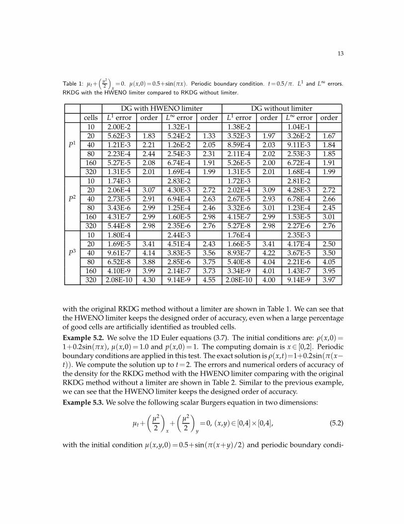
with the initial condition µ(x,0) = 0.5+sin(πx) and periodic boundary conditions. Wecompute the solution up to t= 0.5/π, when the solution is still smooth. The errors andnumerical orders of accuracy for the RKDG method with the HWENO limiter comparing

13

Table 1: µt+(

µ2

2

)

x= 0. µ(x,0)= 0.5+sin(πx). Periodic boundary condition. t= 0.5/π. L1 and L∞ errors.

RKDG with the HWENO limiter compared to RKDG without limiter.

DG with HWENO limiter DG without limiter

cells L1 error order L∞ error order L1 error order L∞ error order

10 2.00E-2 1.32E-1 1.38E-2 1.04E-120 5.62E-3 1.83 5.24E-2 1.33 3.52E-3 1.97 3.26E-2 1.67

P1 40 1.21E-3 2.21 1.26E-2 2.05 8.59E-4 2.03 9.11E-3 1.8480 2.23E-4 2.44 2.54E-3 2.31 2.11E-4 2.02 2.53E-3 1.85160 5.27E-5 2.08 6.74E-4 1.91 5.26E-5 2.00 6.72E-4 1.91320 1.31E-5 2.01 1.69E-4 1.99 1.31E-5 2.01 1.68E-4 1.99

10 1.74E-3 2.83E-2 1.72E-3 2.81E-220 2.06E-4 3.07 4.30E-3 2.72 2.02E-4 3.09 4.28E-3 2.72


10 1.80E-4 2.44E-3 1.76E-4 2.35E-320 1.69E-5 3.41 4.51E-4 2.43 1.66E-5 3.41 4.17E-4 2.50


with the original RKDG method without a limiter are shown in Table 1. We can see thatthe HWENO limiter keeps the designed order of accuracy, even when a large percentageof good cells are artificially identified as troubled cells.

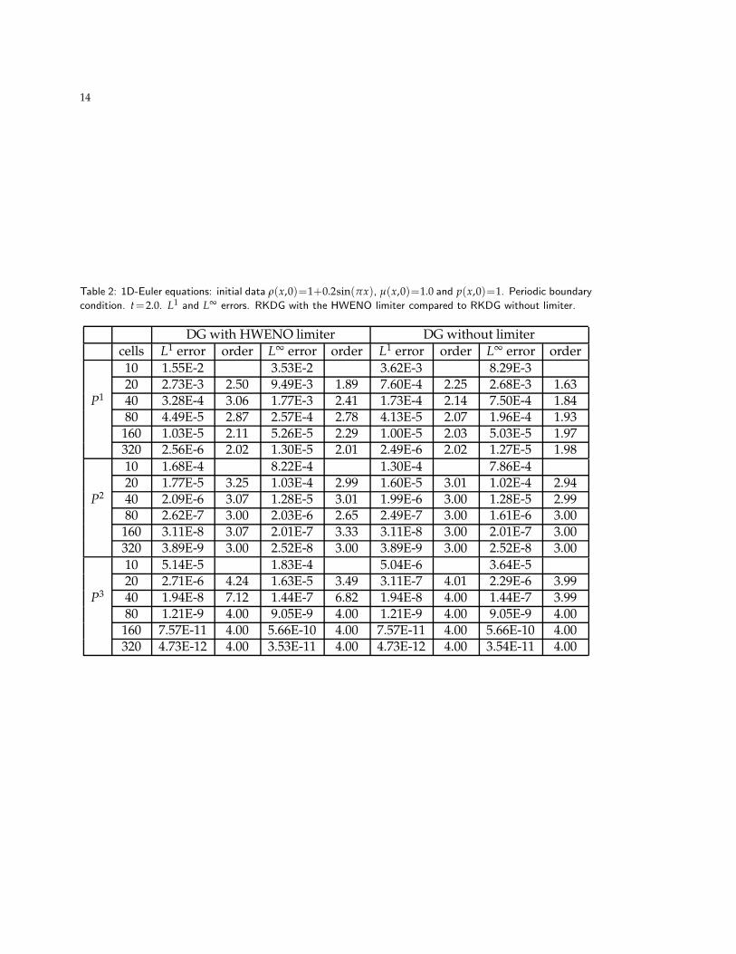
Example 5.2. We solve the 1D Euler equations (3.7). The initial conditions are: ρ(x,0)=1+0.2sin(πx), µ(x,0)= 1.0 and p(x,0)= 1. The computing domain is x∈ [0,2]. Periodicboundary conditions are applied in this test. The exact solution is ρ(x,t)=1+0.2sin(π(x−t)). We compute the solution up to t=2. The errors and numerical orders of accuracy ofthe density for the RKDG method with the HWENO limiter comparing with the originalRKDG method without a limiter are shown in Table 2. Similar to the previous example,we can see that the HWENO limiter keeps the designed order of accuracy.

Example 5.3. We solve the following scalar Burgers equation in two dimensions:

µt+

(

µ2

2

)

x

+

(

µ2

2

)

y

=0, (x,y)∈ [0,4]×[0,4], (5.2)

with the initial condition µ(x,y,0)= 0.5+sin(π(x+y)/2) and periodic boundary condi-

14

Table 2: 1D-Euler equations: initial data ρ(x,0)=1+0.2sin(πx), µ(x,0)=1.0 and p(x,0)=1. Periodic boundary

condition. t=2.0. L1 and L∞ errors. RKDG with the HWENO limiter compared to RKDG without limiter.



10 1.55E-2 3.53E-2 3.62E-3 8.29E-320 2.73E-3 2.50 9.49E-3 1.89 7.60E-4 2.25 2.68E-3 1.63

P1 40 3.28E-4 3.06 1.77E-3 2.41 1.73E-4 2.14 7.50E-4 1.8480 4.49E-5 2.87 2.57E-4 2.78 4.13E-5 2.07 1.96E-4 1.93

160 1.03E-5 2.11 5.26E-5 2.29 1.00E-5 2.03 5.03E-5 1.97320 2.56E-6 2.02 1.30E-5 2.01 2.49E-6 2.02 1.27E-5 1.98

10 1.68E-4 8.22E-4 1.30E-4 7.86E-420 1.77E-5 3.25 1.03E-4 2.99 1.60E-5 3.01 1.02E-4 2.94

P2 40 2.09E-6 3.07 1.28E-5 3.01 1.99E-6 3.00 1.28E-5 2.9980 2.62E-7 3.00 2.03E-6 2.65 2.49E-7 3.00 1.61E-6 3.00

160 3.11E-8 3.07 2.01E-7 3.33 3.11E-8 3.00 2.01E-7 3.00320 3.89E-9 3.00 2.52E-8 3.00 3.89E-9 3.00 2.52E-8 3.00

10 5.14E-5 1.83E-4 5.04E-6 3.64E-520 2.71E-6 4.24 1.63E-5 3.49 3.11E-7 4.01 2.29E-6 3.99

P3 40 1.94E-8 7.12 1.44E-7 6.82 1.94E-8 4.00 1.44E-7 3.9980 1.21E-9 4.00 9.05E-9 4.00 1.21E-9 4.00 9.05E-9 4.00

160 7.57E-11 4.00 5.66E-10 4.00 7.57E-11 4.00 5.66E-10 4.00320 4.73E-12 4.00 3.53E-11 4.00 4.73E-12 4.00 3.54E-11 4.00

15

Table 3: µt+(

µ2

2

)

x+(

µ2

2

)

y=0. µ(x,y,0)=0.5+sin(π(x+y)/2). Periodic boundary condition. t=0.5/π. L1

and L∞ errors. RKDG with the HWENO limiter compared to RKDG without limiter.



10×10 3.99E-2 3.27E-1 3.19E-2 3.40E-120×20 9.78E-3 2.03 1.20E-1 1.44 7.88E-3 2.02 1.05E-1 1.68

P1 40×40 2.31E-3 2.08 3.28E-2 1.87 1.98E-3 1.99 3.26E-2 1.6980×80 5.34E-4 2.11 9.10E-3 1.85 4.92E-4 2.01 9.16E-3 1.83

160×160 1.23E-4 2.12 2.38E-3 1.93 1.23E-4 2.00 2.40E-3 1.93

10×10 5.04E-3 1.77E-1 5.20E-3 1.81E-120×20 8.16E-4 2.62 4.13E-2 2.09 8.29E-4 2.64 4.15E-2 2.12

P2 40×40 1.12E-4 2.86 6.08E-3 2.77 1.12E-4 2.88 6.03E-3 2.7880×80 1.44E-5 2.96 1.00E-3 2.60 1.44E-5 2.96 1.00E-3 2.59

160×160 1.82E-6 2.98 1.37E-4 2.86 1.82E-6 2.98 1.37E-4 2.86

10×10 1.91E-3 8.22E-2 1.91E-3 8.29E-220×20 1.25E-4 3.93 9.16E-3 3.16 1.29E-4 3.89 9.21E-3 3.17

P3 40×40 8.97E-6 3.80 7.57E-4 3.60 9.11E-6 3.82 7.51E-4 3.6180×80 5.80E-7 3.95 5.93E-5 3.67 5.76E-7 3.98 6.03E-5 3.64

160×160 3.65E-8 3.99 3.97E-6 3.90 3.65E-8 3.98 3.97E-6 3.92

tions in both directions. We compute the solution up to t= 0.5/π, when the solution isstill smooth. The errors and numerical orders of accuracy for the RKDG method with theHWENO limiter comparing with the original RKDG method without limiter are shownin Table 3. We again observe good results as in the one-dimensional case.

Example 5.4. We solve the Euler equations (4.4). The initial conditions are: ρ(x,y,0) =1+0.2sin(π(x+y)), µ(x,y,0)=0.7, ν(x,y,0)=0.3, p(x,y,0)=1. The computational domainis (x,y)∈ [0,2]×[0,2]. Periodic boundary conditions are applied in both directions. Theexact solution is ρ(x,y,t)= 1+0.2sin(π(x+y−t)). We compute the solution up to t= 2.The errors and numerical orders of accuracy of the density for the RKDG method with theHWENO limiter comparing with the original RKDG method without a limiter are shownin Table 4. The proposed HWENO limiter again keeps the designed order of accuracy.

We now test the performance of the RKDG method with the HWENO limiters forproblems containing shocks. From now on, we reset the constant to Ck=1. For compari-son with the RKDG method using the minmod TVB limiter, we refer to the results in [4,7].For comparison with the RKDG method using the previous versions of HWENO typelimiters, we refer to the results in [18, 30].

Example 5.5. We consider the 1D Euler equations (3.7) with a Riemann initial con-

16

Table 4: 2D-Euler equations: initial data ρ(x,y,0) = 1+0.2sin(π(x+y)), µ(x,y,0) = 0.7, ν(x,y,0) = 0.3, and

p(x,y,0)=1. Periodic boundary condition. t=2.0. L1 and L∞ errors. RKDG with the HWENO limiter comparedto RKDG without limiter.



10×10 4.16E-2 7.98E-2 2.55E-2 4.44E-220×20 5.61E-3 2.89 1.81E-2 2.13 3.72E-3 2.78 7.71E-3 2.52

P1 40×40 7.83E-4 2.84 3.80E-3 2.25 5.29E-4 2.81 1.51E-3 2.3580×80 1.17E-4 2.73 7.02E-4 2.44 9.14E-5 2.53 4.73E-4 1.67

160×160 2.49E-5 2.24 1.63E-4 2.10 1.89E-5 2.27 1.30E-4 1.86

10×10 7.94E-4 5.71E-3 7.95E-4 5.52E-320×20 1.06E-4 2.90 9.23E-4 2.63 1.02E-4 2.95 8.78E-4 2.65

P2 40×40 1.34E-5 2.98 1.43E-4 2.69 1.25E-5 3.03 1.28E-4 2.7780×80 1.48E-6 3.17 1.70E-5 3.07 1.49E-6 3.07 1.70E-5 2.91

160×160 1.81E-7 3.04 2.17E-6 2.97 1.81E-7 3.04 2.17E-6 2.97

10×10 4.10E-4 9.86E-4 4.86E-5 6.70E-420×20 2.85E-6 7.16 4.04E-5 4.60 2.85E-6 4.08 4.04E-5 4.05

P3 40×40 1.75E-7 4.02 2.49E-6 4.02 1.75E-7 4.03 2.49E-6 4.0280×80 1.08E-8 4.01 1.55E-7 4.01 1.08E-8 4.02 1.55E-7 4.01

160×160 6.76E-10 4.00 9.71E-9 4.00 6.76E-10 4.00 9.71E-9 4.00

17

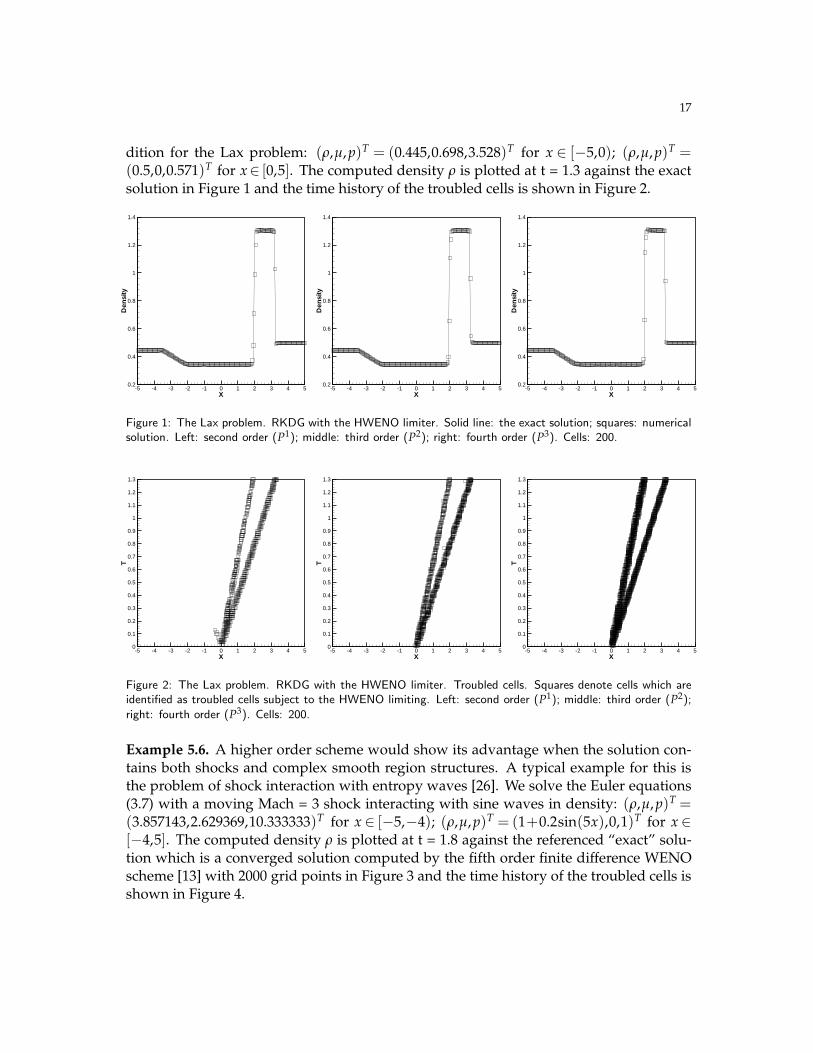
dition for the Lax problem: (ρ,µ,p)T = (0.445,0.698,3.528)T for x ∈ [−5,0); (ρ,µ,p)T =(0.5,0,0.571)T for x∈ [0,5]. The computed density ρ is plotted at t = 1.3 against the exactsolution in Figure 1 and the time history of the troubled cells is shown in Figure 2.

X

Den

sity

-5 -4 -3 -2 -1 0 1 2 3 4 50.2

0.4

0.6

0.8

1

1.2

1.4

X

Den

sity

-5 -4 -3 -2 -1 0 1 2 3 4 50.2

0.4

0.6

0.8

1

1.2

1.4

X

Den

sity

-5 -4 -3 -2 -1 0 1 2 3 4 50.2

0.4

0.6

0.8

1

1.2

1.4

Figure 1: The Lax problem. RKDG with the HWENO limiter. Solid line: the exact solution; squares: numericalsolution. Left: second order (P1); middle: third order (P2); right: fourth order (P3). Cells: 200.

X

T

-5 -4 -3 -2 -1 0 1 2 3 4 50

0.1

0.2

0.3

0.4

0.5

0.6

0.7

0.8

0.9

1

1.1

1.2

1.3

X

T

-5 -4 -3 -2 -1 0 1 2 3 4 50

0.1

0.2

0.3

0.4

0.5

0.6

0.7

0.8

0.9

1

1.1

1.2

1.3

X

T

-5 -4 -3 -2 -1 0 1 2 3 4 50

0.1

0.2

0.3

0.4

0.5

0.6

0.7

0.8

0.9

1

1.1

1.2

1.3

Figure 2: The Lax problem. RKDG with the HWENO limiter. Troubled cells. Squares denote cells which areidentified as troubled cells subject to the HWENO limiting. Left: second order (P1); middle: third order (P2);

right: fourth order (P3). Cells: 200.

Example 5.6. A higher order scheme would show its advantage when the solution con-tains both shocks and complex smooth region structures. A typical example for this isthe problem of shock interaction with entropy waves [26]. We solve the Euler equations(3.7) with a moving Mach = 3 shock interacting with sine waves in density: (ρ,µ,p)T =(3.857143,2.629369,10.333333)T for x ∈ [−5,−4); (ρ,µ,p)T = (1+0.2sin(5x),0,1)T for x ∈[−4,5]. The computed density ρ is plotted at t = 1.8 against the referenced “exact” solu-tion which is a converged solution computed by the fifth order finite difference WENOscheme [13] with 2000 grid points in Figure 3 and the time history of the troubled cells isshown in Figure 4.

18

X

Den

sity

-5 -4 -3 -2 -1 0 1 2 3 4 50.5

1

1.5

2

2.5

3

3.5

4

4.5

X

Den

sity

-5 -4 -3 -2 -1 0 1 2 3 4 50.5

1

1.5

2

2.5

3

3.5

4

4.5

X

Den

sity

-5 -4 -3 -2 -1 0 1 2 3 4 50.5

1

1.5

2

2.5

3

3.5

4

4.5

Figure 3: The shock density wave interaction problem. RKDG with the HWENO limiter. Solid line: the “exact”solution; squares: numerical solution. Left: second order (P1); middle: third order (P2); right: fourth order

(P3). Cells: 200.

X

T

-5 -4 -3 -2 -1 0 1 2 3 4 50

0.1

0.2

0.3

0.4

0.5

0.6

0.7

0.8

0.9

1

1.1

1.2

1.3

1.4

1.5

1.6

1.7

1.8

X

T

-5 -4 -3 -2 -1 0 1 2 3 4 50

0.1

0.2

0.3

0.4

0.5

0.6

0.7

0.8

0.9

1

1.1

1.2

1.3

1.4

1.5

1.6

1.7

1.8

X

T

-5 -4 -3 -2 -1 0 1 2 3 4 50

0.1

0.2

0.3

0.4

0.5

0.6

0.7

0.8

0.9

1

1.1

1.2

1.3

1.4

1.5

1.6

1.7

1.8

Figure 4: The shock density wave interaction problem. RKDG with the HWENO limiter. Troubled cells. Squaresdenote cells which are identified as troubled cells subject to the HWENO limiting. Left: second order (P1);

middle: third order (P2); right: fourth order (P3). Cells: 200.

19

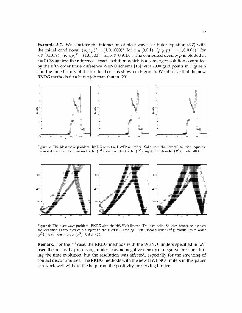
Example 5.7. We consider the interaction of blast waves of Euler equation (3.7) withthe initial conditions: (ρ,µ,p)T = (1,0,1000)T for x ∈ [0,0.1); (ρ,µ,p)T = (1,0,0.01)T forx∈ [0.1,0.9); (ρ,µ,p)T =(1,0,100)T for x∈ [0.9,1.0]. The computed density ρ is plotted att = 0.038 against the reference “exact” solution which is a converged solution computedby the fifth order finite difference WENO scheme [13] with 2000 grid points in Figure 5and the time history of the troubled cells is shown in Figure 6. We observe that the newRKDG methods do a better job than that in [29].

X

Den

sity

0 0.2 0.4 0.6 0.8 10

1

2

3

4

5

6

7

X

Den

sity

0 0.2 0.4 0.6 0.8 10

1

2

3

4

5

6

7

X

Den

sity

0 0.2 0.4 0.6 0.8 10

1

2

3

4

5

6

7

Figure 5: The blast wave problem. RKDG with the HWENO limiter. Solid line: the ”exact” solution; squares:numerical solution. Left: second order (P1); middle: third order (P2); right: fourth order (P3). Cells: 400.

X

T

0 0.2 0.4 0.6 0.8 10

0.01

0.02

0.03

X

T

0 0.2 0.4 0.6 0.8 10

0.01

0.02

0.03

X

T

0 0.2 0.4 0.6 0.8 10

0.01

0.02

0.03

Figure 6: The blast wave problem. RKDG with the HWENO limiter. Troubled cells. Squares denote cells whichare identified as troubled cells subject to the HWENO limiting. Left: second order (P1); middle: third order

(P2); right: fourth order (P3). Cells: 400.

Remark. For the P3 case, the RKDG methods with the WENO limiters specified in [29]used the positivity-preserving limiter to avoid negative density or negative pressure dur-ing the time evolution, but the resolution was affected, especially for the smearing ofcontact discontinuities. The RKDG methods with the new HWENO limiters in this papercan work well without the help from the positivity-preserving limiter.

20

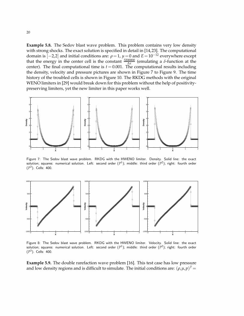
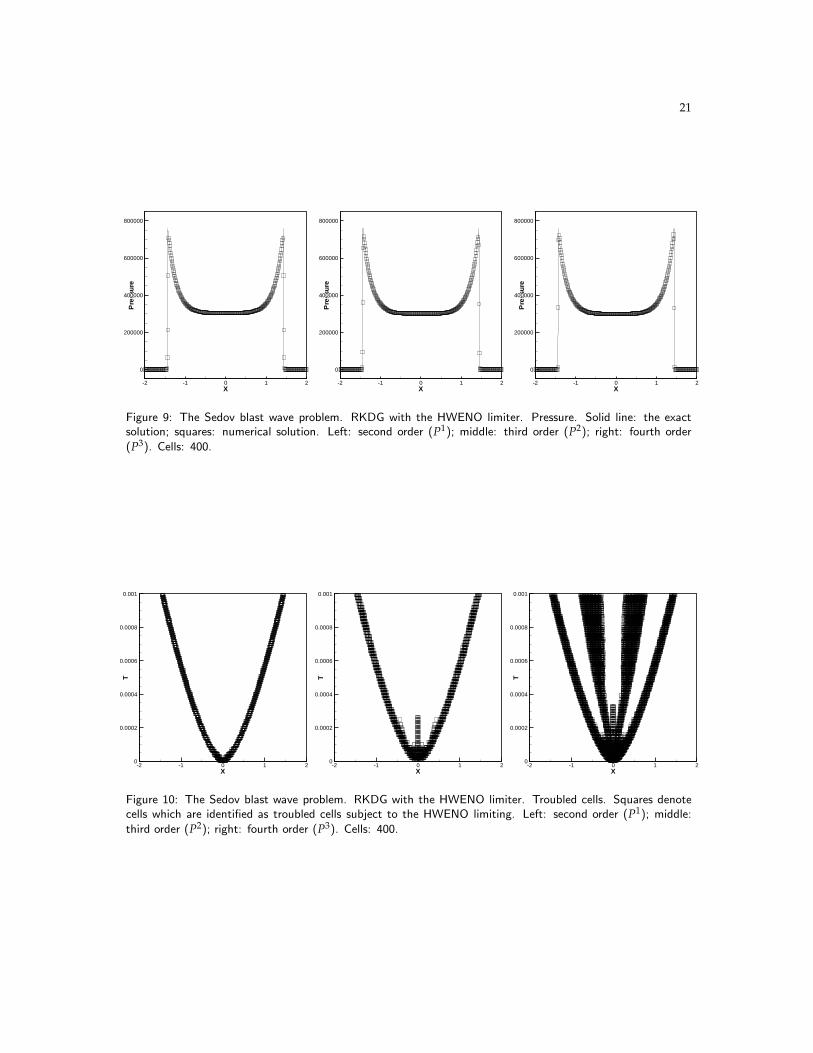
Example 5.8. The Sedov blast wave problem. This problem contains very low densitywith strong shocks. The exact solution is specified in detail in [14,23]. The computationaldomain is [−2,2] and initial conditions are: ρ=1, µ=0 and E=10−12 everywhere exceptthat the energy in the center cell is the constant 3200000

∆x (emulating a δ-function at thecenter). The final computational time is t= 0.001. The computational results includingthe density, velocity and pressure pictures are shown in Figure 7 to Figure 9. The timehistory of the troubled cells is shown in Figure 10. The RKDG methods with the originalWENO limiters in [29] would break down for this problem without the help of positivity-preserving limiters, yet the new limiter in this paper works well.

X

Den

sity

-2 -1 0 1 2

0

1

2

3

4

5

6

7

X

Den

sity

-2 -1 0 1 2

0

1

2

3

4

5

6

7

X

Den

sity

-2 -1 0 1 2

0

1

2

3

4

5

6

7

Figure 7: The Sedov blast wave problem. RKDG with the HWENO limiter. Density. Solid line: the exactsolution; squares: numerical solution. Left: second order (P1); middle: third order (P2); right: fourth order

(P3). Cells: 400.

X

Vel

oci

ty

-2 -1 0 1 2-1000

-500

0

500

1000

X

Vel

oci

ty

-2 -1 0 1 2-1000

-500

0

500

1000

X

Vel

oci

ty

-2 -1 0 1 2-1000

-500

0

500

1000

Figure 8: The Sedov blast wave problem. RKDG with the HWENO limiter. Velocity. Solid line: the exactsolution; squares: numerical solution. Left: second order (P1); middle: third order (P2); right: fourth order(P3). Cells: 400.

Example 5.9. The double rarefaction wave problem [16]. This test case has low pressureand low density regions and is difficult to simulate. The initial conditions are: (ρ,µ,p)T=

21

X

Pre

ssu

re

-2 -1 0 1 2

0

200000

400000

600000

800000

X

Pre

ssu

re

-2 -1 0 1 2

0

200000

400000

600000

800000

X

Pre

ssu

re

-2 -1 0 1 2

0

200000

400000

600000

800000

Figure 9: The Sedov blast wave problem. RKDG with the HWENO limiter. Pressure. Solid line: the exactsolution; squares: numerical solution. Left: second order (P1); middle: third order (P2); right: fourth order

(P3). Cells: 400.

X

T

-2 -1 0 1 20

0.0002

0.0004

0.0006

0.0008

0.001

X

T

-2 -1 0 1 20

0.0002

0.0004

0.0006

0.0008

0.001

X

T

-2 -1 0 1 20

0.0002

0.0004

0.0006

0.0008

0.001

Figure 10: The Sedov blast wave problem. RKDG with the HWENO limiter. Troubled cells. Squares denotecells which are identified as troubled cells subject to the HWENO limiting. Left: second order (P1); middle:

third order (P2); right: fourth order (P3). Cells: 400.

22

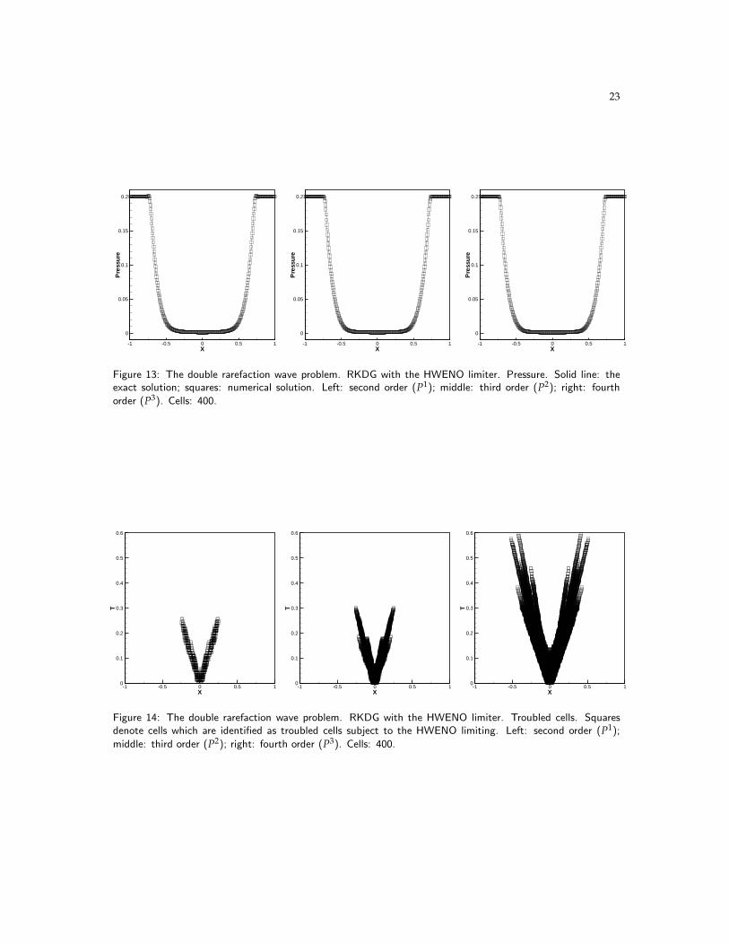
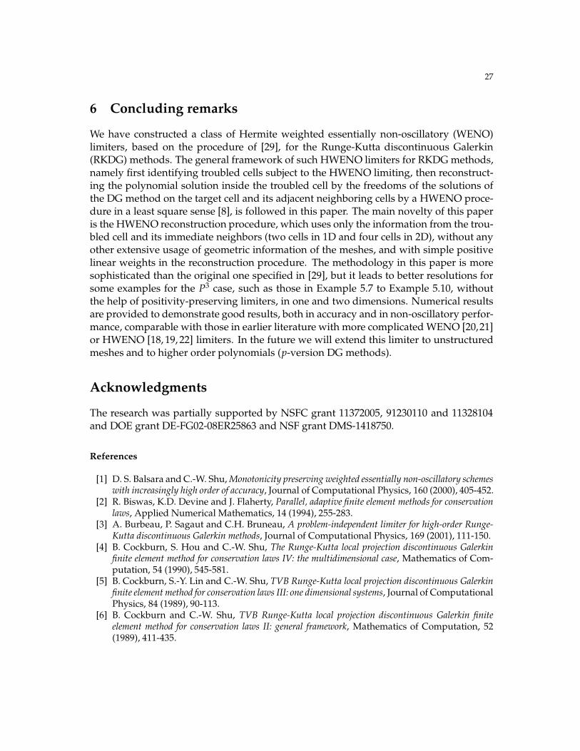
(7,−1,0.2)T for x∈ [−1,0); (ρ,µ,p)T=(7,1,0.2)T for x∈ [0,1]. The final computational timeis t=0.6. The computational results including the density, velocity and pressure picturesare shown in Figure 11 to Figure 13. The time history of the troubled cells is shown inFigure 14. For the P3 case, the RKDG methods with the WENO limiters in [29] do notwork for this problem without the help of positivity-preserving limiters, however thesame RKDG methods with the new HWENO limiters in this paper produce good results.

X

Den

sity

-1 -0.5 0 0.5 10

1

2

3

4

5

6

7

X

Den

sity

-1 -0.5 0 0.5 10

1

2

3

4

5

6

7

X

Den

sity

-1 -0.5 0 0.5 10

1

2

3

4

5

6

7

Figure 11: The double rarefaction wave problem. RKDG with the HWENO limiter. Density. Solid line: theexact solution; squares: numerical solution. Left: second order (P1); middle: third order (P2); right: fourth

order (P3). Cells: 400.

X

Vel

oci

ty

-1 -0.5 0 0.5 1

-1

-0.5

0

0.5

1

X

Vel

oci

ty

-1 -0.5 0 0.5 1

-1

-0.5

0

0.5

1

X

Vel

oci

ty

-1 -0.5 0 0.5 1

-1

-0.5

0

0.5

1

Figure 12: The double rarefaction wave problem. RKDG with the HWENO limiter. Velocity. Solid line: theexact solution; squares: numerical solution. Left: second order (P1); middle: third order (P2); right: fourth


Example 5.10. Double Mach reflection problem. This model problem is originally from[28]. We solve the Euler equations (4.4) in a computational domain of [0,4]×[0,1]. Thereflection boundary condition is used at the wall, which for the rest of the bottom bound-ary (the part from x= 0 to x= 1

6 ), the exact post-shock condition is imposed. At the top

23

X

Pre

ssu

re

-1 -0.5 0 0.5 1

0

0.05

0.1

0.15

0.2

X

Pre

ssu

re

-1 -0.5 0 0.5 1

0

0.05

0.1

0.15

0.2

X

Pre

ssu

re

-1 -0.5 0 0.5 1

0

0.05

0.1

0.15

0.2

Figure 13: The double rarefaction wave problem. RKDG with the HWENO limiter. Pressure. Solid line: theexact solution; squares: numerical solution. Left: second order (P1); middle: third order (P2); right: fourth


X

T

-1 -0.5 0 0.5 10

0.1

0.2

0.3

0.4

0.5

0.6

X

T

-1 -0.5 0 0.5 10

0.1

0.2

0.3

0.4

0.5

0.6

X

T

-1 -0.5 0 0.5 10

0.1

0.2

0.3

0.4

0.5

0.6

Figure 14: The double rarefaction wave problem. RKDG with the HWENO limiter. Troubled cells. Squaresdenote cells which are identified as troubled cells subject to the HWENO limiting. Left: second order (P1);

middle: third order (P2); right: fourth order (P3). Cells: 400.

24

boundary is the exact motion of the Mach 10 shock. The results shown are at t = 0.2.Three different orders of accuracy for the RKDG with HWENO limiters, k=1, k=2 andk=3 (second order, third order and fourth order), are used in the numerical experiments.The simulation results are shown in Figure 15. The “zoomed-in” pictures around thedouble Mach stem to show more details are given in Figure 16. The troubled cells identi-fied at the last time step are shown in Figure 17. Clearly, the resolution improves with anincreasing k on the same mesh.

X

Y

0 1 2 30

0.5

1

X

Y

0 1 2 30

0.5

1

X

Y

0 1 2 30

0.5

1

Figure 15: Double Mach refection problem. RKDG with the HWENO limiter. 30 equally spaced density contoursfrom 1.5 to 21.5. Top: second order (P1); middle: third order (P2); bottom: fourth order (P3). Cells: 800 ×200.

25

X

Y

2 2.50

0.25

0.5

X

Y

2 2.50

0.25

0.5

X

Y

2 2.50

0.25

0.5

Figure 16: Double Mach refection problem. RKDG with HWENO limiter. Zoom-in pictures around the Machstem. 30 equally spaced density contours from 1.5 to 21.5. Left: second order (P1); right: third order (P2);

bottom: fourth order (P3). Cells: 800 × 200.

26

X

Y

0 1 2 30

0.5

1

X

Y

0 1 2 30

0.5

1

X

Y

0 1 2 30

0.5

1

Figure 17: Double Mach refection problem. RKDG with the HWENO limiter. Troubled cells. Squares denotecells which are identified as troubled cells subject to the HWENO limiting. Top: second order (P1); middle:

third order (P2); bottom: fourth order (P3). Cells: 800 × 200.

27

6 Concluding remarks

We have constructed a class of Hermite weighted essentially non-oscillatory (WENO)limiters, based on the procedure of [29], for the Runge-Kutta discontinuous Galerkin(RKDG) methods. The general framework of such HWENO limiters for RKDG methods,namely first identifying troubled cells subject to the HWENO limiting, then reconstruct-ing the polynomial solution inside the troubled cell by the freedoms of the solutions ofthe DG method on the target cell and its adjacent neighboring cells by a HWENO proce-dure in a least square sense [8], is followed in this paper. The main novelty of this paperis the HWENO reconstruction procedure, which uses only the information from the trou-bled cell and its immediate neighbors (two cells in 1D and four cells in 2D), without anyother extensive usage of geometric information of the meshes, and with simple positivelinear weights in the reconstruction procedure. The methodology in this paper is moresophisticated than the original one specified in [29], but it leads to better resolutions forsome examples for the P3 case, such as those in Example 5.7 to Example 5.10, withoutthe help of positivity-preserving limiters, in one and two dimensions. Numerical resultsare provided to demonstrate good results, both in accuracy and in non-oscillatory perfor-mance, comparable with those in earlier literature with more complicated WENO [20,21]or HWENO [18, 19, 22] limiters. In the future we will extend this limiter to unstructuredmeshes and to higher order polynomials (p-version DG methods).

Acknowledgments

The research was partially supported by NSFC grant 11372005, 91230110 and 11328104and DOE grant DE-FG02-08ER25863 and NSF grant DMS-1418750.

References

[1] D. S. Balsara and C.-W. Shu, Monotonicity preserving weighted essentially non-oscillatory schemeswith increasingly high order of accuracy, Journal of Computational Physics, 160 (2000), 405-452.

[2] R. Biswas, K.D. Devine and J. Flaherty, Parallel, adaptive finite element methods for conservationlaws, Applied Numerical Mathematics, 14 (1994), 255-283.

[3] A. Burbeau, P. Sagaut and C.H. Bruneau, A problem-independent limiter for high-order Runge-Kutta discontinuous Galerkin methods, Journal of Computational Physics, 169 (2001), 111-150.

[4] B. Cockburn, S. Hou and C.-W. Shu, The Runge-Kutta local projection discontinuous Galerkinfinite element method for conservation laws IV: the multidimensional case, Mathematics of Com-putation, 54 (1990), 545-581.

[5] B. Cockburn, S.-Y. Lin and C.-W. Shu, TVB Runge-Kutta local projection discontinuous Galerkinfinite element method for conservation laws III: one dimensional systems, Journal of ComputationalPhysics, 84 (1989), 90-113.

[6] B. Cockburn and C.-W. Shu, TVB Runge-Kutta local projection discontinuous Galerkin finiteelement method for conservation laws II: general framework, Mathematics of Computation, 52(1989), 411-435.

28

[7] B. Cockburn and C.-W. Shu, The Runge-Kutta discontinuous Galerkin method for conservationlaws V: multidimensional systems, Journal of Computational Physics, 141 (1998), 199-224.

[8] M. Dumbser, D.S. Balsara, E.F. Toro and C.D. Munz, A unified framework for the constructionof one-step finite-volume and discontinuous Galerkin schemes on unstructured meshes, Journal ofComputational Physics, 227 (2008), 8209-8253.

[9] M. Dumbser and M. Kaser, Arbitrary high order non-oscillatory finite volume schemes on un-structured meshes for linear hyperbolic systems, Journal of Computational Physics, 221 (2007),693-723.

[10] M. Dumbser, O. Zanotti, R. Loubere and S. Diot, A posteriori subcell limiting of the discontin-uous Galerkin finite element method for hyperbolic conservation laws, Journal of ComputationalPhysics, 278 (2014), 47-75.

[11] O. Friedrichs, Weighted essentially non-oscillatory schemes for the interpolation of mean values onunstructured grids, Journal of Computational Physics, 144 (1998), 194-212.

[12] C. Hu and C.-W. Shu, Weighted essentially non-oscillatory schemes on triangular meshes, Journalof Computational Physics, 150 (1999), 97-127.

[13] G. Jiang and C.-W. Shu, Efficient implementation of weighted ENO schemes, Journal of Compu-tational Physics, 126 (1996), 202-228.

[14] V.P. Korobeinikov, Problems of Point-Blast Theory, American Institute of Physics, 1991.[15] L. Krivodonova, J. Xin, J.-F. Remacle, N. Chevaugeon and J.E. Flaherty, Shock detection and

limiting with discontinuous Galerkin methods for hyperbolic conservation laws, Applied Numeri-cal Mathematics, 48 (2004), 323-338.

[16] T. Linde, P.L. Roe, Robust Euler codes, in: 13th Computational Fluid Dynamics Conference,AIAA Paper-97-2098.

[17] X. Liu, S. Osher and T. Chan, Weighted essentially non-oscillatory schemes, Journal of Compu-tational Physics, 115 (1994), 200-212.

[18] H. Luo, J.D. Baum and R. Lohner, A Hermite WENO-based limiter for discontinuous Galerkinmethod on unstructured grids, Journal of Computational Physics, 225 (2007), 686-713.

[19] J. Qiu and C.-W. Shu, Hermite WENO schemes and their application as limiters for Runge-Kuttadiscontinuous Galerkin method: one dimensional case, Journal of Computational Physics, 193(2003), 115-135.

[20] J. Qiu and C.-W. Shu, Runge-Kutta discontinuous Galerkin method using WENO limiters, SIAMJournal on Scientific Computing, 26 (2005), 907-929.

[21] J. Qiu and C.-W. Shu, A comparison of troubled-cell indicators for Runge-Kutta discontinuousGalerkin methods using weighted essentially nonoscillatory limiters, SIAM Journal on ScientificComputing, 27 (2005), 995-1013.

[22] J. Qiu and C.-W. Shu, Hermite WENO schemes and their application as limiters for Runge-Kuttadiscontinuous Galerkin method II: two dimensional case, Computers and Fluids, 34 (2005), 642-663.

[23] L.I. Sedov, Similarity and Dimensional Methods in Mechanics, Academic Press, New York,1959.

[24] C.-W. Shu, Essentially non-oscillatory and weighted essentially non-oscillatory schemes for hyper-bolic conservation laws, In Advanced Numerical Approximation of Nonlinear HyperbolicEquations, B. Cockburn, C. Johnson, C.-W. Shu and E. Tadmor (Editor: A. Quarteroni), Lec-ture Notes in Mathematics, volume 1697, Springer, 1998, 325-432.

[25] C.-W. Shu and S. Osher, Efficient implementation of essentially non-oscillatory shock-capturingschemes, Journal of Computational Physics, 77 (1988), 439-471.

[26] C.-W. Shu and S. Osher, Efficient implementation of essentially non-oscillatory shock capturing

29

schemes II, Journal of Computational Physics, 83 (1989), 32-78.[27] C. Wang, X. Zhang, C.-W. Shu and J. Ning, Robust high order discontinuous Galerkin schemes for

two-dimensional gaseous detonations, Journal of Computational Physics, 231 (2012), 653-665.[28] P. Woodward and P. Colella, The numerical simulation of two-dimensional fluid flow with strong

shocks, Journal of Computational Physics, 54 (1984), 115-173.[29] X. Zhong and C.-W. Shu, A simple weighted essentially nonoscillatory limiter for Runge-Kutta

discontinuous Galerkin methods, Journal of Computational Physics, 232 (2013), 397-415.[30] J. Zhu, J. Qiu, C.-W. Shu and M. Dumbser, Runge-Kutta discontinuous Galerkin method using

WENO limiters II: Unstructured meshes, Journal of Computational Physics, 227 (2008), 4330-4353.

[31] J. Zhu, X. Zhong, C.-W. Shu and J.X. Qiu, Runge-Kutta discontinuous Galerkin method usinga new type of WENO limiters on unstructured meshes, Journal of Computational Physics, 248(2013), 200-220.

runge-kuttadiscontinuous galerkinmethod witha …zhongxh/paper/hweno.pdfthe runge-kutta...

Documents