SIMULATING DIOXANE TRANSPORT IN A HETEROGENEOUS GLACIAL

AQUIFER SYSTEM (WASHTENAW COUNTY, MICHIGAN) USING PUBLICLY

AVAILABLE MODELS AND DATA

By

Rungroj Benjakul

A THESIS

Submitted in partial fulfillment of the requirements for the degree of

MASTER OF SCIENCE IN GEOLOGY

MICHIGAN TECHNOLOGICAL UNIVERSITY

2010

© 2010 Rungroj Benjakul

This thesis, “Simulating Dioxane Transport in a Heterogeneous Glacial Aquifer

System (Washtenaw County, Michigan) Using Publicly Available Models and Data,” is

hereby approved in partial fulfillment of the requirements for the Degree of MASTER

OF SCIENCE IN GEOLOGY.

DEPARTMENT: Geological and Mining Engineering and Sciences

Signatures: Thesis Advisor _________________________________________

John S. Gierke

Department Chair _________________________________________

Wayne D. Pennington

Date _________________________________________

3

ABSTRACT

The primary challenge in groundwater and contaminant transport modeling is

obtaining the data needed for constructing, calibrating and testing the models. Large

amounts of data are necessary for describing the hydrostratigraphy in areas with complex

geology. Increasingly states are making spatial data available that can be used for input to

groundwater flow models. The appropriateness of this data for large-scale flow systems

has not been tested. This study focuses on modeling a plume of 1,4-dioxane in a

heterogeneous aquifer system in Scio Township, Washtenaw County, Michigan. The

analysis consisted of: (1) characterization of hydrogeology of the area and construction of

a conceptual model based on publicly available spatial data, (2) development and

calibration of a regional flow model for the site, (3) conversion of the regional model to a

more highly resolved local model, (4) simulation of the dioxane plume, and (5)

evaluation of the model's ability to simulate field data and estimation of the possible

dioxane sources and subsequent migration until maximum concentrations are at or below

the Michigan Department of Environmental Quality's residential cleanup standard for

groundwater (85 ppb). MODFLOW-2000 and MT3D programs were utilized to simulate

the groundwater flow and the development and movement of the 1,4-dioxane plume,

respectively. MODFLOW simulates transient groundwater flow in a quasi-3-dimensional

sense, subject to a variety of boundary conditions that can simulate recharge, pumping,

and surface-/groundwater interactions. MT3D simulates solute advection with

groundwater flow (using the flow solution from MODFLOW), dispersion, source/sink

mixing, and chemical reaction of contaminants. This modeling approach was successful

at simulating the groundwater flows by calibrating recharge and hydraulic conductivities.

The plume transport was adequately simulated using literature dispersivity and sorption

coefficients, although the plume geometries were not well constrained.

4

ACKNOWLEDGEMENT I am highly grateful to my advisor, Professor John S. Gierke, for his kind

guidance, encouragement, and support for this research. Many thanks are due to Dr.

Remigio H. Galárraga-Sánchez and Dr. Aleksey Smirnov for serving as my thesis

committee. Special thank to Tyler Fincher for helping me in dealing with English

difficulty and review my thesis writing. I would also like to acknowledge my gratitude to

the Royal Thai Government for providing me a great opportunity to study in the United

States with full financial support. I am grateful to the Department of Geological and

Mining Engineering and Sciences and Michigan Technological University for having me

here.

I would also like to extend special thanks to Kelly Mclean and Amie Ledgerwood

for all their office and registration help, Miriam Rioz Sanchez and Rudiger Escobar Wolf

for helping with the GIS data processing, my fellow students: Elisa Piispa, Claudia Toro,

Anna Colvin, Edrick Ramos, Anieri Morales, Carla Alonso and many others for all

supports and friendship. My willingness to put forward everyday was supported by

encouraging words from family and friends. Lastly, I offer my regards and blessings to

all of those who supported me in any respect during the completion of the thesis.

5

TABLE OF CONTENTS

ABSTRACT ....................................................................................................................... 3

ACKNOWLEDGEMENT ................................................................................................ 4

LIST OF TABLES ............................................................................................................ 7

LIST OF FIGURES .......................................................................................................... 8

1. INTRODUCTION ...................................................................................................... 10

BACKGROUND ............................................................................................................ 10

STUDY SITE ................................................................................................................ 13

Geology ................................................................................................................. 15

Climate .................................................................................................................. 18

1,4-DIOXANE .............................................................................................................. 19

Environmental fate ................................................................................................ 20

Toxicology ............................................................................................................. 21

Regulatory Standards............................................................................................ 21

PURPOSE, OBJECTIVES, AND SCOPE ............................................................................ 22

2. METHODS ................................................................................................................. 23

CONCEPTUAL FLOW MODEL ...................................................................................... 24

Boundary Conditions ............................................................................................ 26

REGIONAL FLOW MODEL ........................................................................................... 29

Steady State Simulation......................................................................................... 29

Model calibration.................................................................................................. 30

Sensitivity Analysis................................................................................................ 32

LOCAL MODELING ...................................................................................................... 33

TRANSPORT MODELING .............................................................................................. 35

Advection............................................................................................................... 36

Dispersion ............................................................................................................. 37

Diffusion ................................................................................................................ 37

Retardation ........................................................................................................... 38

6

Potential Sources of Contamination ..................................................................... 39

3. RESULTS .................................................................................................................... 41

CONCEPTUAL MODEL ................................................................................................. 41

REGIONAL FLOW MODEL ........................................................................................... 42

Steady State Flow .................................................................................................. 42

Model Calibration ................................................................................................. 43

Sensitivity Analysis................................................................................................ 47

LOCAL FLOW MODEL ................................................................................................. 48

TRANSPORT MODEL .................................................................................................... 52

Potential Sources of Contamination ..................................................................... 52

4. DISCUSSION ............................................................................................................. 55

HYDROGEOLOGIC SETTING ......................................................................................... 56

GROUNDWATER FLOW MODEL ................................................................................... 56

TRANSPORT MODEL ................................................................................................... 56

LIMITATION AND UNCERTAINTY ................................................................................ 57

FUTURE WORK ........................................................................................................... 58

5. CONCLUSIONS ......................................................................................................... 61

REFERENCES ................................................................................................................ 62 

SUPPLEMENTARY DATA .............................................................................. CD-ROM

7

LIST OF TABLES 

TABLE 1.1 SUMMARY OF THE GEOLOGIC SETTING OF THE WESTERN PLUME AREA ............ 17

TABLE 1.2 CHARACTERISTIC AND PROPERTIES OF DIOXANE .............................................. 20

TABLE 2.1 SUMMARY OF THE HYDROGEOLOGY OF THE CONCEPTUAL MODEL .................... 25

TABLE 2.2 RIVER BOUNDARY CONDITION PARAMETERS .................................................... 27

TABLE 2.3 GROUNDWATER RECHARGE VALUES ASSIGNED DURING CALIBRATION PROCESS

......................................................................................................................... 31

TABLE 3.1 SIMULATED WATER BUDGET FOR THE CALIBRATED REGIONAL FLOW MODEL ... 46

TABLE 3.2 SUMMARY OF CALIBRATED PARAMETER VALUES FOR THE REGIONAL MODEL... 47

TABLE 3.3 SUMMARY OF CALIBRATED PARAMETER VALUES AND SENSITIVITIES FOR THE

LOCAL MODEL .................................................................................................. 52

TABLE 4.1 COMPARISON OF THE PUBLISHED MODELS TO THIS STUDY ................................ 55

8

LIST OF FIGURES

FIGURE 1.1 SELECTED IMPORTANT FEATURES IN THE STUDY AREA .................................... 11

FIGURE 1.2 LOCATION MAP OF THE STUDY AREA ............................................................... 14

FIGURE 1.3 TOPOGRAPHIC MAP OF THE STUDY AREA ......................................................... 14

FIGURE 1.4 SURFICIAL GEOLOGY OF WASHTENAW COUNTY ............................................. 17

FIGURE 1.5 ANNUAL PRECIPITATION DATA AT UNIVERSITY OF MICHIGAN WEATHER

STATION ID 200231 ........................................................................................ 18

FIGURE 1.6 ANNUAL TEMPERATURE DATA AT UNIVERSITY OF MICHIGAN WEATHER

STATION ID 200231 ........................................................................................ 19

FIGURE 1.7 STRUCTURE OF DIOXANE ................................................................................. 19

FIGURE 2.1 REGIONAL MODEL DOMAIN OF THE CONCEPTUAL MODEL ................................ 25

FIGURE 2.2 TOP VIEW OF REGIONAL MODEL EXTENT SHOWING LATERAL GRID SPACING AND

BOUNDARY CONDITIONS .................................................................................. 27

FIGURE 2.3 GROUNDWATER RECHARGE ZONES, EASTINGS AND NORTHINGS ARE IN FEET . 28

FIGURE 2.4 SEPTEMBER 1995 POTENTIOMETRIC SURFACE MAP OF UPPER AQUIFER .......... 31

FIGURE 2.5 LOCAL MODEL EXTENT SHOWING BOUNDARY CONDITIONS ............................. 34

FIGURE 2.6 APRIL, 1988 DELINEATION MAP OF DIOXANE CONCENTRATION IN UPPER

AQUIFER ......................................................................................................... 40

FIGURE 3.1 TOP ELEVATION CONTOUR MAP OF THE LOWER CONFINING LAYER ................ 42

FIGURE 3.2 STEADY STATE POTENTIOMETRIC SURFACE MAP (REGIONAL MODEL LAYER 2,

CONTOURS ARE IN FEET AMSL, EASTINGS AND NORTHINGS ARE IN FEET) ........ 43

FIGURE 3.3 PLOT OF COMPUTED VERSUS OBSERVED HEADS FOR UPPER AQUIFER UNIT IN

REGIONAL FLOW MODEL .................................................................................. 44

FIGURE 3.4 PLOT OF RESIDUAL VERSUS OBSERVED HEADS FOR UPPER AQUIFER UNIT IN

REGIONAL FLOW MODEL. ................................................................................. 45

FIGURE 3.5 RELATIVE COMPOSITE SENSITIVITY OF CALIBRATED PARAMETERS .................. 48

FIGURE 3.6 STEADY STATE POTENTIOMETRIC SURFACE MAP (LOCAL MODEL LAYER 2,

CONTOURS ARE IN FEET AMSL, EASTINGS AND NORTHINGS ARE IN FEET) ........ 49

FIGURE 3.7 PLOT OF COMPUTED VERSUS OBSERVED HEADS FOR UPPER AQUIFER UNIT IN

LOCAL FLOW MODEL. ...................................................................................... 50

9

FIGURE 3.8 PLOT OF RESIDUAL VERSUS OBSERVED HEADS FOR UPPER AQUIFER UNIT IN

REGIONAL FLOW MODEL. ................................................................................. 51

FIGURE 3.9 SIMULATED PLUME DELINEATION MAP IN LOWER AQUIFER WITH INITIAL

CONDITION ...................................................................................................... 53

FIGURE 3.10 CALIBRATED PLUME DELINEATION MAP IN LOWER AQUIFER ........................ 54 

10

1. Introduction Background

Groundwater contamination by 1,4-dioxane (hereinafter called dioxane) has been

a concern of government and residents in Washtenaw County, Michigan for almost four

decades. Dioxane is harmful to humans’ health and found to be stable in water (Agency

for Toxic Substances and Disease Registry: ATSDR, 2007). To date, more than a

hundred private water wells are contaminated by dioxane released from the Pall Life

Sciences (PLS), formerly Gelman Sciences. The Michigan Department of Environmental

Quality (MDEQ, 2004) reported that dioxane was used by PLS between 1966 and 1986

to produce medical filters. Disposal method and waste handling during this period

resulted in a discharge of dioxane into groundwater. However, the volume of released

wastewater and the concentration of the chemical are unknown, which consequently

results in uncertainty of the mass-loading history of the area.

Contamination in the wells was first discovered in the fall of 1985 and a

comprehensive site investigation started later in 1986 (MDEQ, 2004). The contaminant

mapping activities delineated the Core System, the Western System, and the Evergreen

System (Figure 1.1). The Core System is the source of contamination, with the

concentrations in excess of 500 ppb (µg/L), spans all of the PLS property, wastewater

seepage ponds, and surrounding area.

This study focuses on the dioxane plume (also known as the Western Plume)

located to the west of a larger area impacted by groundwater contamination in Scio

Township, Washtenaw County, Michigan. According to the Consent Judgment, the

Western System (or the Western Plume area) is the area of groundwater contamination

west, northwest or southwest of the Core System. Thus, the Western Plume area (Figure

1.1) refers to the western area of the PLS site, extending to the confluence of the Honey

Creek Tributaries and reaching from a northern extent along Interstate Highway I-94 one

mile to the south. The Western System was initially believed to be emanating from the

Core System contamination. After the additional site investigation, the perception of this

11

area was changed. The Western Plume then has been interpreted separately from the Core

System (MDEQ, 2004).

Figure 1.1 Selected important features in the study area (created from MDEQ 2004 and digital data of Michigan Geographic Framework, Michigan Center for Geographic Information). The areas impacted by dioxane contamination include the Core System, the Marshy System, the Western System, the Evergreen System Area, Artesian Well Area and the Dupont Circle Area. The yellow star represents the center of the Western System.

Geologic complexity and limitation in subsurface data are always challenges in

analyzing the behavior of a groundwater system. Groundwater modeling is generally

considered a valuable approach for describing and/or predicting groundwater flow and

contaminant fate and transport. It has been used at many hazardous waste sites with

varying degrees of success. Therefore groundwater models were developed for the

Western Plume area to better understand the subsurface behavior. The three dimensional

(3D) groundwater model developed by Brode (2002) was built to examine the role of

12

groundwater and surface water interactions with the development of the groundwater

contamination in the study area. It consisted of four model layers representing two

aquifers bounded by two confining layers. The model was calibrated with data from eight

observation wells in the Western Plume area. An advective transport of dissolved dioxane

from Little Lake was simulated using MODPATH (Pollack, 1944), a particle-tracking

(advection only) post-processing model, to determine the travel pathways and transport

history.

Later, Cypher and Lemke (2009) constructed three alternative conceptual models

coupled with the possible locations where the contaminant enters the groundwater to

enhance the perception of the aquifer system and reduce the model uncertainty. The

analysis was composed of four major procedures: (1) construction of the alternative

models for a site, (2) calibration of the models based on the same dataset, (3) ranking the

viability of the models using various criteria, and (4) evaluation model appropriateness.

The authors utilized the MODFLOW-2000 and MODPATH programs to simulate

groundwater flow in the conceptual models and evaluate the transport pathway,

respectively. After running all models under steady state condition, the models were

calibrated using the potentiometric surface of the static water level data in September

1995, which is the date before the remediation at the site was implemented. The authors

also examined the sensitivity of the models to small changes in model parameters and

boundary conditions. As a result, the contaminated Core System area, i.e., the holding

ponds and Third Sister Lake, were identified as the most probable sources of the Western

Plume. Nevertheless, further refinement of the conceptual and numerical model was

suggested for this area based on additional publically available data and more

mechanistically sophisticated transport modeling.

Regional modeling studies of groundwater contamination have not been common

due to the inherent complexity of computer modeling and the dearth of data for many

sites. Lack of field investigation data for studying contaminant behavior is always a

challenge for contaminant transport modeling. State laws and local ordinances require

that hydrogeological data be collected and reported for domestic water purposes, both for

private and community supplies, as well as for construction, industrial and agricultural

13

purposes. Prior to the prevalence of geographical information systems (GIS), this data

was filed away, often in non-centralized fashion, making data gathering problematic.

Currently, however, hydrogeological information for water supply purposes is commonly

archived in publically accessible sites, typically maintained by state departments of

environmental quality/natural resources. In addition, even information on contaminated

sites (contaminant concentrations in soils and groundwater) are available. The goal of this

work is to use publically available data to construct regional and local models of

groundwater flow and contaminant transport for a field site where modeling was

performed previously using fewer data sources. The objective is to demonstrate that the

publically available data can be used with publically available models to adequately

simulate field conditions in a complex glacial aquifer system contaminated with 1,4-

dioxane. The site conditions and important contaminant properties are outlined below.

Study Site

This study focused on the contamination in a shallow aquifer of the Western

Plume System located in Scio Township, Washtenaw County, Michigan as shown in

Figure 1.2. The Sister Lakes and the Honey Creek and its tributary are the significant

hydrographic features in the area (Figure 1.2). The Western Plume System is one of the

areas impacted by dioxane contamination released from the PLS located on Wagner Road

(Figure 1.1). The topography of this area ranges from 940 feet above mean sea level

(amsl) in the vicinity of the PLS property to the lower area of approximately 850 feet

amsl at the Honey Creek (Figure 1.3). Five major aquifers are identified in the area: the

Core System, the Western System, the Evergreen System, the Marshy System, and the

Unit E aquifer (MDEQ, 2004). These aquifers can be grouped as shallow and deep

aquifers. The Unit E aquifer is only a deep aquifer in this area. A significant pumping

remediation in the Core System area started in 1997, twelve years after the contamination

was first discovered.

14

Figure 1.2 Location map of the study area, Eastings and Northings are in feet.

Figure 1.3 Topographic map of the study area, Eastings and Northings are in feet.

Honey Creek

PLS Property

Western Plume area

15

The public data related to the study site can be accessible through the state

government website. The current and historical information on the investigation and

remediation of groundwater contamination are provided by the Michigan Department of

Natural Resources and Environment (MDNRE). Selected documents, letters, and maps

are downloadable on the MDNRE website. The Michigan Center for Geographic

Information (MCGI) provides several statewide datasets concerning aerial imagery,

census, geology, groundwater, hydrography, hydrology, land cover, land use, political

features, soils, topography, transportation and much more through the Michigan

Geographic Data Library. The library consists of several data format with various spatial

and temporal resolutions. The data are categorized and can be sorted based on geographic

extent or theme type.

There are two previous studies primarily concerning the contamination in the

Western Plume area (Brode, 2002; Cypher and Lemke, 2009). Brode (2002) investigated

the effect of an interaction between groundwater and surface water on the development of

dioxane plume in the Western Plume area by using a numerical model. The numerical

model was based on a four-layered conceptual model. Cypher and Lemke (2009)

established alternative conceptual models to describe the hydrogeologic complexity of

this area and the four-layered conceptual model was also included in the study. Both

studies utilized MODPATH to simulate an advective transport of dioxane from the

potential source locations. Brode indicated that the Little Lake served as a source of the

Western Plume. In contrast, Cypher and Lemke (2009) concluded that the dioxane was

possibly released from the Third Sister Lake and the hydrogeologic complexity played

the important role in the groundwater system behavior.

Geology

The geology of Washtenaw County can be categorized into two major groups:

unconsolidated sediments (glacial drift deposits) and bedrock. The bedrock is primarily

sedimentary rocks with a thickness of 1.2 to 2.1 kilometers. The glacial deposits overlie

the bedrock, primarily the Coldwater Shale, across nearly all the county (Fleck, 1980).

The Coldwater Shale is relatively impermeable and has a maximum thickness of more

than 300 meters. The glacial deposits are composed of lakebeds, outwash, deltas and

16

moraines. Moraines are a combination of clay, silt, sand, and gravel. Outwash is

composed of mostly sand and gravel. Moraines and outwash cover the majority of the

county. Figure 1.4 illustrates a surficial geology map of Washtenaw County showing the

Western Plume area location. Glacial lithology cannot be regionally correlated in the

subsurface possibly due to the heterogeneity of glacial deposits. Aquifers in the glacial

deposits mostly consist of sands and gravels and vary regionally in thickness and

permeability. Twenter et al. (1976) categorized the glacial deposits of Washtenaw County

as a combination of aquifer and non-aquifer materials. Aquifer units consist of permeable

materials. Non-aquifer units include clay, hardpan, and heterogeneous fine-grained

deposits with low permeability.

In the Western Plume area, the top elevation of the Coldwater Shale is

approximately 720 feet amsl. Above the bedrock are the glacial deposits, which generally

are low to medium permeable clay or till (Fleck, 1980). Till is fine to coarse grained and

presents in moraines and till plains. The Western Plume area is located along the

northwestern flank of the Fort Wayne Moraine. Its surface geology is characterized by

glacial outwash sands and gravels, terminal moraine ablation tills, and compacted ground

moraine tills. The thickness of glacial drift in the Western Plume area ranges from

approximately 130 to 250 feet (Cypher, 2008). The stratigraphy of the deposits is quite

complex. The influences of the cycles of erosion and deposition of the successive glacial

episodes resulted in a lack of continuity of these units. However, there are at least 5

distinct deposits associated with the Western Plume area (Brode, 2002) as summarized in

Table 1.1.

17

Figure 1.4 Surficial Geology of Washtenaw County (created from digital data of 1982 Quaternary geology maps of northern and southern Michigan, Michigan Center for Geographic Information).

Table 1.1 Summary of the geologic setting of the Western Plume area

Description Type Composition Top elevation

(feet amsl) Thickness

(feet) Top

Fine-grained deposit

Confining layer

Diamictons: reddish-brown to grey clayey silts and are commonly interbeded with sands and gravels

Highest at 1069

Generally < 20

Upper sand and gravel

Aquifer (both confined and unconfined)

Primarily coarse sands and various amounts of gravel with some finer-grained sands and silts.

~ 840-940 Less than 40 to 160

Fine-grained deposit

Confining layer

Primarily diamicton: grey silty clay or clayey silt having a massive texture and traces of sand and gravel

~ 760-860 ~ 15-120

Lower sand and gravel

Aquifer Generally coarse sands with various amounts of gravel.

~ 740-780 ~ 20 - 50

Bottom

Coldwater Shale Formation:

Bedrock grey to bluish-grey shale with very low permeability

Average ~ 720 ~ 500 - 1300

18

Climate

The study area is located in the Southeast Lower climate division (Eichenlaub et

al., 1990). Climate data for the period 1980 to 2007, the period relevant to this

investigation, was obtained from the online climate data directory (NOAA 2009). Annual

precipitation data acquired from the University of Michigan Weather Station (Station ID

200230) for the period from 1966 through 2008 is provided in Figure 1.5. The average

annual precipitation for this period was approximately 35.5 inches (902 mm), with the

highest precipitation mostly occurring during the month of June and the lowest amount in

February. The average annual mean temperature of the area between 1966 and 2008 was

approximately 49.5 Fº (9.7 ºC) (Figure 1.6)

Figure 1.5 Annual precipitation data at University of Michigan Weather Station ID 200231.

19

Figure 1.6 Annual temperature data at University of Michigan Weather Station ID

200231.

1,4-Dioxane

1,4-Dioxane is produced from the dehydration of ethylene glycol and is a strong

acid catalyst. It has been used for a wide variety of industrial purposes such as a

purification of prescriptions, production of dye, and textile finishing. It is generally used

as a solvent stabilizer (USEPA, 2006; Mohr, 2010). Dioxane (also known as diethylene

ether, diethylene dioxide, p-dioxane, and glycol ethylene ether) is a highly stable

synthetic organic compound (Mohr, 2001). It is miscible and highly mobile in

groundwater. The molecular formula of dioxane is C4H8O2, which has a molecular weight

of 88.10 g/mole. The chemical structure of dioxane is shown in Figure 1.7. The physical

and chemical properties and the characteristics of dioxane are listed in Table 1.2.

Figure 1.7 Structure of dioxane.

20

Table 1.2 Characteristic and properties of dioxane

Characteristic/Property Value

Chemical Abstracts Service Registry Number (CASRN) 123-91-1 EPA Hazardous Waste Identification Number U108 Color Clear Physical State Flammable liquid, colorlessOdor Faint pleasant odor Molecular Formula C4H8O2 Molecular Weight 88.1 Molar volume 85.8 cm3/mole at 25 C Melting Point 11.80C at 760 mm Hg Boiling Point 101.1C at 760 mm Hg Heat of vaporization 98.6 cal/g Water Solubility mg/L at 20C Miscible Density 1.0329 g/mL at 20C Vapor Density (air = 1) 3.03 Evaporation rate 2.42 Viscosity at 20C 0.012 poise Soil-water partition coefficient, KOC 1.23 Log of octanol-water partition coefficient (Log KOW) -0.27 Vapor Pressure 30 mm Hg at 20C Flash Point 5-18C at 760 mm Hg Henry's Law Constant, KH 4.88 x 10-6 atm m3/mole Ultraviolet light absorption maximum 180 nm Source: ASTDR 2007, EPA 2006, Mohr 2010 Note: atm = atmosphere; cal = calories; g = grams; L = liter; mL = milliliters; mm Hg = millimeters of mercury; mg = milligrams; nm = nanometers; C = degrees Celsius

Environmental fate

Since dioxane is a highly soluble compound, it is very mobile and migrates

rapidly in groundwater. Its high solubility, low Henry’s Law Constant, and low log Kow

result in a slight retardation (ATSDR, 2007; Mohr, 2010). The study of Priddle and

Jackson (1991) suggests that retardation factors (Rf) based on field data, correlation

estimates, and column data are from 1.0 to 1.6. Biodegradability of dioxane has been

studied since the early 1960s (Fincher and Payne, 1962). Many studies have reported that

dioxane is not significantly biodegradable (Abe, 1999; USEPA, 2006; Lesage et al.,

21

1990; Skadsen et al., 2004). Most of these studies were conducted under aerobic

biodegradation. Dioxane was not degradable under anaerobic conditions in two studies

(Adams et al., 1994; Steffan, 2006). The cyclic-ether structure of dioxane is believed to

be a key of its resistance to natural biodegradation (Grady et al., 1997). Nevertheless,

Howard (1991) indicated that the half-life of dioxane in groundwater based on estimated

non-acclimated aqueous aerobic biodegradation is 56 to 360 days.

Toxicology

Dioxane enters the human body by inhalation, ingestion, and dermal contact.

Short-term exposure may cause eye, nose, and throat irritation. Exposure to large

amounts of dioxane can cause kidney and liver damage and eventually death. Liver and

kidney toxicity are the health effects resulted from a long-term exposure. Dioxane is

categorized in Group B2 (probable human) carcinogen. Two studies have revealed liver

cancer in laboratory rats with exposure to the chemical (ATSDR, 2007; Goldsworthy et

al., 1991). Although there is no case of carcinogenicity in humans, it is believed that

cancer may occur in humans as well. The length and quantity of exposure to dioxane are

the factors that control the possible health effects on humans.

Regulatory Standards

Dioxane concentration criteria for drinking water and groundwater vary state by

state, between 3 and 85 μg/L. Michigan does not list a Maximum Contaminant Level

(MCL) for dioxane. At the time of the contaminant discovery, the standard for

groundwater was 3 parts per billion (ppb1). The State relaxed the generic residential

cleanup criteria to 77 ppb in 1994 (MDEQ, 2004). The current residential cleanup

standard for groundwater regulated by Michigan Department of Environmental Quality is

85 ppb and has been used since June 2000.

1 At dilute concentrations in water, such as those common to groundwater contamination, 1 ppb is

practically equal to 1 µg/L.

22

Purpose, Objectives, and Scope

The primary objective of this study was to simulate the dioxane fate and transport

in the Western Plume area. Publicly available spatial data were obtained and analyzed to

characterize the hydrogeology of the area and develop the regional conceptual model.

The construction of the conceptual model was based on the four-layered models in the

prior studies. The simulation of groundwater flow and contaminant transport was

accomplished by utilizing a sophisticated computer modeling approach. MODFLOW-

2000 was selected as the groundwater flow modeling code for this study. A combination

of advection, dispersion, and sorption were introduced to the transport model by using

MT3D program. In addition, the potential sources and subsequent migration of dioxane

plume were assessed. The historical plume movement was estimated until the maximum

concentrations diminish to the MDEQ's cleanup standard (85 ppb) or less.

23

2. Methods MODFLOW, the most widely-used groundwater flow model developed by the

McDonald and Harbaugh (1988) of the U.S. Geological Survey, was utilized in this

analysis to simulate the 3-dimensional, regional and local groundwater flows in the

aquifer system. In order to more efficiently develop the MODFLOW models,

Groundwater Modeling System (GMS) version 6.5 was selected for operating

MODFLOW-2000 input and output in this study. The GMS program is a pre and post

processor with a graphical user interface, developed by Aquaveo, LLC in Provo, Utah.

This program was chosen because it supports a 3D finite difference modeling with the

MODFLOW-2000 (saturated zone) and a simple 3D transport with MT3DMS. The

program also provides a conceptual modeling approach, a useful tool for constructing a

complex 3D stratigraphy and a conceptual model. The MT3DMS is a new version of the

Modular 3-Dimensional Transport model (MT3D) developed by Zheng and Wang

(Zheng and Wang, 1999). The program provides an additional function to cope with a

multi-species transport.

Data utilized in this study was collected from publicly available sources, most of

which are accessible on the internet. All Geographic Information System (GIS) data

relevant to the site, e.g., topographic map, Digital Elevation Model (DEM), borehole

data, Quaternary geology, hydrographic features, estimated groundwater recharge, and

legislative political boundaries were obtained from a digital database of the Michigan

Geographic Data Library. The historical and current information of the contaminated site

such as well information and historical sampling data are available on the Michigan

Department of Natural Resources and Environment website. In addition, the National

Oceanic and Atmospheric Administration (NOAA) provided the meteorological data,

including temperature and precipitation, for the study area.

Once all required data were obtained and properly processed for use in the

modeling, identification of spatial model parameters and data analysis were undertaken in

order to understand the aquifer system and contaminant transport. To accomplish the goal

of this study, the analysis consisted of five primary steps: (1) characterization of

24

hydrogeology of the area and construction of a conceptual model based on publicly

available spatial data, (2) development and calibration of a regional flow model for the

site, (3) conversion of the regional model to a more highly resolved local model, (4)

simulation of the dioxane plume, and (5) evaluation of the model's ability to simulate

field data and estimation of the possible dioxane sources and subsequent migration until

maximum concentrations are at or below the Michigan Department of Environmental

Quality's residential cleanup standard for groundwater (85 ppb).

Conceptual Flow Model

A conceptual flow model is a basic graphical representation of the characteristics

of the groundwater flow system that are important in developing the numerical model

(Anderson and Woessner, 1992). The conceptual model provides the framework of the

state of the flow system, horizontal and vertical boundaries of the model, and interaction

with sources and sinks of water. Development of the conceptual model requires a review

of literature and data regarding the aquifer system and groundwater flow in the study

area.

The regional model domain of the study site covers an area of 65.5 square miles,

including all of Scio Township, the northern parts of Lodi and Pittsfield Townships and

the western part of Ann Arbor Township (Figure 2.1). The real-world coordinate of the

southwest corner of the regional model is (13,250,000 ft East, 272,000 ft North) using the

State Plane North American Datum 1983, Michigan South Zone 2113 coordinate system.

The coordinate of the northeast corner of the model is (13,300,000 ft East, 308,500 ft

North). This regional model consists of four layers representing the glacial drift deposits

in the area, including two confining layers and two aquifers as summarized in Table 2.1.

Layer 1, the Upper Confining Layer (UCL), represents deposits above the Upper Aquifer

(UA), layer 2. These deposits are primary diamicton (mixed particle-sized sediments),

fill, and clays. Layer 2 represents the UA, which is of primary interest to this study. Layer

3 (Lower Confining Layer, LCL) is a confining layer that separates the Upper Aquifer

and Lower Aquifer (LA). Layer 4 represents the LA, another aquifer overlying the

bedrock surface. Shale bedrock is treated as a no-flow boundary.

25

Figure 2.1 Regional model domain of the conceptual model, Eastings and Northings are in feet.

Table 2.1 Summary of the hydrogeology of the conceptual model

Model Unit

Description Type Composition Elevation range

(feet amsl)

Top 1 Upper Confining

Layer (UCL) Confining layer

Primarily diamicton, fill, and clay

710-1071

2 Upper Aquifer

(UA)

Aquifer (present under both

confined and unconfined conditions)

Primarily sand and gravel

663-1025

3 Lower Confining

Layer (LCL) Confining layer

Primarily diamicton and clay

654-953

Bottom 4 Lower Aquifer

(LA) Aquifer

Primarily sand and gravel

600-884

26

The hydrogeologic interpretation was based on the reported lithology along with

the static water level and previous four-layered conceptual models of Brode (2002) and

Cypher (2008). The hydrostratigraphy of the model was defined by using 19 borehole

logs from the Cypher (2008) study, coupled with 139 borehole logs (Figure 2.1) and the

DEM from the Michigan Geographic Data Library. The materials in each borehole were

subdivided into four hydrogeologic classes and assigned the numerical values

corresponding to the layer types. The Inversed Distance Weighting (IDW) interpolation

method was utilized to delineate layer geometries for the model.

Boundary Conditions

The Huron River is a main hydrographic feature that influences the regional

groundwater system in this area. A discharge of regional groundwater flow to the Huron

River was first hypothesized by Healy (2005). At a local scale, the groundwater system is

recharged by or discharges to surface water bodies, including lakes and small streams in

the study area. Thus, two types of boundary conditions were applied to the model.

All of the perennially hydrographic features, such as Huron River, Mill Creek,

First Sister Lake, Second Sister Lake, Third Sister Lake, Honey Creek and its tributaries,

were treated as river boundaries (Figure 2.2). When the river attribute is assigned to an

object, three river parameters are required: elevation, stage, and conductance. River stage

was obtained from the topographic map. River elevation and conductance values are

consistent with the study of Cypher (2008). Since there are no data characterizing the

river bottom thickness and its vertical hydraulic conductivity has been determined for all

surface water bodies in the model domain, the conductance was treated as a fitting

parameter in the model. River-bed elevations were approximated with a constant of five

feet below the river stage for the Huron River, Mill Creek, and Honey Creek. The Honey

Creek tributary (HCT) was assigned the river bed elevation of 2-feet below its river stage.

The depth of the First Sister Lake is 12 feet, whereas the Second Sister Lakes is 25 feet.

The Third Sister Lake is approximately 55 feet deep (Ball, 1947; Hammer and Stoermer,

1997; Bridgeman et al., 2000; Potzger and Wilson, 1941). The specified parameter values

of the river boundaries are shown in Table 2.2.

27

Figure 2.2 Top view of regional model extent showing lateral grid spacing and boundary

conditions, Eastings and Northings are in feet. The red grid cells are “inactive” and correspond to areas outside the regional flow system for the area south of Huron River.

Table 2.2 River boundary condition parameters

River Stage (feet amsl) River Bottom (feet amsl) Conductance (ft2/day)

Huron River 835 – 750 830 – 745 2500

Mill Creek 855 – 830 850 – 825 1250

Honey Creek 885 – 800 880 – 795 1250

HCT 922 – 852 920 – 850 625

1st Sister Lake 902 890 625

2nd Sister Lake 905 880 2500

3rd Sister Lake 905 850 312

Inactive (No-flow) Active CellRiver Boundary

28

In addition to the river boundary, no-flow boundaries were assigned to the

Coldwater Shale bedrock, the western, southern, and eastern borders of the model

domain. All cells north of the Huron River were designated inactive since the Huron

River is assumed as a ground water divide (Figure 2.2). Nine groundwater recharge zones

(Figure 2.3) with respect to different recharge rates ranged from 4 to 12 inches per year

were applied across the uppermost active cells. The groundwater recharge data in the

study site was obtained from digital map data from the Michigan Geographical Data

Library, which contains state-wide estimates of groundwater recharge. Accuracy of the

data is +/- 0.092 ft/yr. The digital map data was derived from a study of groundwater

recharge, a part of Groundwater Inventory and Mapping Project which is a collaboration

of the MDEQ, United States Geological Survey (USGS), and Michigan State University

(MDEQ, 2006). The recharge values were calculated from observed baseflow by using a

statistical regression technique (MDEQ, 2006). The baseflow is assumed to be equal to

groundwater recharge in a shallow glacial aquifer.

Figure 2.3 Groundwater recharge zones, Eastings and Northings are in feet.

29

Regional Flow Model

Steady State Simulation

Steady state flow is the condition when heads do not change with time. Therefore,

the head gradient, flow velocity, and flow direction are constant. The finite-difference

regional model grid consisted of 100 columns and 100 rows. The grid lines are oriented

in a north-south, east-west fashion. The uniform grid spacing along the x-axis and y-axis

are 500 and 365 feet, respectively. There are 4 model layers from a depth of 650 to 1,100

feet with a total of 28,048 active cells. The thickness and boundaries of each grid layer

was adjusted with regard to the layer ranges of each unit in the conceptual model. Figure

2.2 illustrates the regional model extent and the lateral grid spacing of the model domain.

The parameter values assigned to the model were based on published data and

were consistent with the values used by Brode (2002) and Cypher (2008). All parameters

except hydraulic conductivity were uniformly assigned to all active cells in the model

domain including an assumed porosity of 0.3, specific yield of 0.2, and specific storage of

3·10-6 ft-1. Initial groundwater levels for the simulation were set to a small distance below

ground surface in order to foster numerical stability. Initial hydraulic conductivity values

vary amongst the model layers. One conductivity value was uniformly applied to each

layer. The conductivity values used by Brode (2002) and Cypher (2008) in the previous

studies were tentatively assigned as the initial parameter values for the calibration

simulations. These values are consistent with the values derived from aquifer pumping

test results reported by PLS and the published report and data (Fleck, 1980; Freeze and

Cherry, 1979; MDEQ, 2004; PLS, 2004; PLS, 2006).

The numerical flow model relied upon the following assumptions:

1. Flow in the aquifer is governed by Darcy’s Law of water movement through

porous media. Mass and energy were conserved. These assumptions are valid over the

scale at which this model is constructed. The solution of the 3-D groundwater flow

equation used in MODFLOW is calculated from the following partial differential

equation (Harbaugh et al., 2000):

( ) ( ) ( )xx yy zz s

h h h hK K K W S

x x y y z z t

(2.1)

30

where Kxx, Kyy, and Kzz are values of hydraulic conductivity along the x, y, and z

coordinate axes, which are assumed to be parallel to the major axes of

hydraulic conductivity (LT-1);

h is the potentiometric head (L);

W is a volumetric flux per unit volume representing sources and/or sinks of water,

with a negative number represents flow out of the groundwater system, and a

positive number for flow in (T-1);

Ss is the specific storage of the porous media (L-1); and

t is time (T).

2. Water density and viscosity are constant over time and space.

3. Hydraulic conductivity in each layer is isotropic in both horizontal and vertical

directions.

Model calibration

After running the model under steady-state conditions, the model was calibrated

using the potentiometric surface derived from the static water level data (hydraulic heads)

in September 1995, which is the time before any significant remedial pumping started at

the site (Brode, 2002; Cypher, 2008). The calibration process is necessary to enhance the

consistency between the numerical model and the observed system (Anderson and

Woessner, 1992). Model calibration is the process of adjusting uncertain model

parameters to improve the agreement between the simulated results and the observed data

and to increase the model reliability.

In this study, the hydraulic conductivity and recharge were adjusted to modify the

head gradient directions and minimize the mean head residual. The remaining parameters

were kept constant. The range of hydraulic conductivity values assigned to the aquifer

units was 50 to 250 ft/day, which is consistent with glacial outwash sand and gravel

deposits (Fetter, 2001). The confining layers were assigned much lower hydraulic

conductivity values between 0.005 and 0.5 ft/day, regarding the range of permeability

values for till consisting of silty sands, to allow a two-order of magnitude difference in

the conductivity between the aquifer and confining units. The recharge values assigned

31

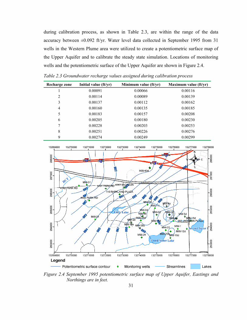
during calibration process, as shown in Table 2.3, are within the range of the data

accuracy between ±0.092 ft/yr. Water level data collected in September 1995 from 31

wells in the Western Plume area were utilized to create a potentiometric surface map of

the Upper Aquifer and to calibrate the steady state simulation. Locations of monitoring

wells and the potentiometric surface of the Upper Aquifer are shown in Figure 2.4.

Table 2.3 Groundwater recharge values assigned during calibration process

Recharge zone Initial value (ft/yr) Minimum value (ft/yr) Maximum value (ft/yr)

1 0.00091 0.00066 0.00116

2 0.00114 0.00089 0.00139

3 0.00137 0.00112 0.00162

4 0.00160 0.00135 0.00185

5 0.00183 0.00157 0.00208

6 0.00205 0.00180 0.00230

7 0.00228 0.00203 0.00253

8 0.00251 0.00226 0.00276

9 0.00274 0.00249 0.00299

Figure 2.4 September 1995 potentiometric surface map of Upper Aquifer, Eastings and

Northings are in feet.

32

A trial-and-error technique was used in the calibration process to minimize

calibrated statistics. The calibrated statistics, including the mean residual head, mean

absolute residual head, and root mean squared (RMS) residual head generated by

MODFLOW, are all based on the residual heads. These statistical values are commonly

determined to evaluate the model calibration. The residual head is the difference between

the simulated head and observed head. The mean residual head is defined as:

Mean residual head = 1

1( )

n

s o ih hn

(2.2)

where hs is the simulated head and ho is the observed head at each observation point. The

sum of residuals is divided by the number of data (n), which were 31 observations in this

case. The mean absolute residual head is the sum of absolute values of the residuals

divided by the number of residuals as defined in equation 2.3.

Mean absolute residual head = 1

1| ( ) |

n

s o ih hn

(2.3)

The mean absolute residual head describes how well a model fits to data while the

mean residual head represents the overall bias in calibration. The RMS is calculated by

taking a square root of the sum of the square of errors for the observations. It is defined

as:

RMS = 0.5

2

1

1| ( ) |

n

s o ih hn

(2.4)

Sensitivity Analysis

Model sensitivity is a reflection of how much the calibrated simulation would

change due to changes in the values of the model inputs. It serves to identify the relative

importance of the measured data to the parameter estimation (Hill and Tiedeman, 2007).

The sensitivity analysis was performed simultaneously with the calibration process. The

analysis consisted of uniformly increasing or decreasing a single model parameter, such

as hydraulic conductivity or recharge, and observing the effects on water-level change

33

statistics and simulated groundwater discharge to the streams. Only one parameter was

changed at a time during the process.

Parameter ESTimation or PEST (Doherty, 2004) was selected for model

optimization and sensitivity analysis in this study. PEST is a software package for

parameter estimation and uncertainty analysis of complex environmental and other

computer models which is alternatively applied as a sensitivity analysis tool in many

hydrological models (Baginska et al., 2003; Bahremand and De Smedt, 2008; Tang et al.,

2007). PEST estimated the best values of a parameter set by minimizing the weighted

sum of the squared residual heads. The sensitivity is simultaneously calculated by using a

nonlinear parameter estimation method. The parameter sensitivity value is expressed by

relative composite sensitivity, which is a byproduct of the parameter estimation. The

relative composite sensitivity of each parameter is useful in determining the effect of the

parameters on the model output when these parameters are of different type and

magnitudes (Doherty, 2004).

Local Modeling

Conversion of a regional scale model to a local scale model is a common

approach to provide more insight and accurate results for groundwater modeling in a

specific locale, particularly in an area where regional groundwater divides and physical

boundaries, such as rock outcrops, streamlines, and lakes, are located far beyond a study

site. Regional-model grid refinement and hydraulic boundaries, i.e., specified head and

no-flow boundary are often utilized to define a new boundary set for constructing a local

model (Anderson and Woessner, 1992; Ebraheem et al., 2004).

In this study, a regional-to-local model conversion was accomplished by using

tools provided by the GMS program. A local-scale model that occupied a small area

within the regional model was developed with grid refinement in a subset of calibrated

regional model. Outputs from the regional model simulation, such as computed heads,

served as the boundary conditions in the local model. The computed head values from the

regional model were assigned as specified head boundaries in the local model. The

regional layer data, including top and bottom elevations, and starting heads, were also

input to the local model.

34

The real-world coordinate of the southwest corner of the local model domain is

(13,267,300 ft East, 281700 ft North) using the Michigan State Plane coordinate system.

The coordinate of the northeast corner of the model is (13,278,300 ft East, 291,800 ft

North). Figure 2.5 illustrated the local model domain with respect to the regional model

boundary. The local model extent covers the 31 monitoring wells in the Western Plume

area and down-gradient area under the range of groundwater flow from the study site

toward the Honey Creek. The finite-different model grid consists of 110 columns and 101

rows. The grid lines are oriented in a north-south, east-west fashion. The grid spacing is

uniform along the x-axis and y-axis with a dimension of 100 feet by 100 feet. There are 4

model layers from depth of 650 to 1,100 feet with a total of 28,968 active cells. The

thickness and boundaries of each grid layer is obtained from the layer data of the regional

model.

Figure 2.5 Local model extent showing boundary conditions, Eastings and Northings are in feet.

35

Hydraulic conductivity in each layer is allowed to be anisotropic in both

horizontal and vertical directions. The horizontal anisotropy2 of hydraulic conductivity is

allowed to range between 0.5 and 1.5. The vertical hydraulic conductivity for each cell is

assigned values that are at or below the horizontal hydraulic conductivity but not less

than one-tenth of the horizontal hydraulic conductivity.

After running the model under steady-state conditions, the model was calibrated

using the same process as conducted on the regional model. The sensitivity of the local

model to the input parameters was also determined as the same manner of the regional

model’s sensitivity analysis. However, the anisotropy of hydraulic conductivity was an

additional parameter included in the local model’s analysis.

Transport Modeling

How dioxane entered the groundwater system in the Western Plume area is still

ambiguous. There is no evidence regarding mass-loading history of dioxane in this area.

Brode (2002) believed that the contamination of the site occurred between 1967 and 1973

when there was an excess runoff from the PLS site to the lower surrounding area. The

concentration of dioxane in the overflow was assumed to be the same as that of the

wastewater at approximately 330 mg/L. On the contrary, Cypher (2008) pointed out that

the most likely source of dioxane in the Western System area is the Third Sister Lake.

However, the assertions of dioxane sources in both studies were based on a transport

model with advective transport process only. In this work the transport modeling was

more sophisticated, as outlined below.

Diffusion, advection, dispersion and retardation are fundamental mechanisms of

solute transport in groundwater (Fetter, 2001). Diffusion is a movement of solutes

regarding concentration gradient from a higher concentration area to a lower

concentration area (Fetter, 1999; Spitz and Moreno, 1996). Advection is a process in

which solutes are carried and transported by flowing groundwater. When the solute is

traveling, it can mix with surrounding water along the flow path, resulting in a dilution of

2 Horizontal anisotropy is defined as the ratio of the hydraulic conductivity in the x-direction

relative to the hydraulic conductivity in the y-direction.

36

the plume. This process is called dispersion. Retardation is a process in which solution

movement is slowed down by sorption and chemical reaction to aquifer materials. The

primary processes of contaminant transport in a groundwater system can be represented

by the following partial differential equation (Zheng and Wang, 1999):

( )( ) ( )ij i s s n

i j i

C CD v C q C R

t x x x

(2.5)

where

θ= porosity of the subsurface medium, dimensionless

C = dissolved concentration (ML-3)

t = time, T

xi,j = distance along the respective Cartesian coordinate axis (L)

Dij = hydrodynamic dispersion coefficient tensor (L2T-1)

vi = seepage or linear pore water velocity (LT-1); it is related to the specific

discharge or Darcy flux through the relationship, vi = qi/θ

qs = volumetric flow rate per unit volume of aquifer representing fluid sources

(positive) and sinks (negative) (T-1)

Cs = concentration of the source or sink flux (ML-3)

ΣRn = chemical reaction term (ML-3T-1).

MT3DMS was utilized in this study because of its capability to develop a

transport model concerning all above processes (Zheng and Wang, 1999). The program

requires the following input parameters with respect to its basic transport package in

order to simulate the dioxane transport in this area:

Advection

Advection is commonly the most influencing process on the contaminant

transport, particularly in highly permeable materials such as sand and gravel. The

advance of solute by advective transport is directly related to the rate of groundwater

flow. According to the Darcy’s law, the rate of groundwater movement in porous media

can be determined in term of average linear velocity. The average linear velocity can be

calculated from the following equation:

37

xe

K dhv

n dl (2.6)

where vx is the average linear velocity (LT-1), K is hydraulic conductivity (LT-1), ne is

effective porosity (dimensionless), and dh/dl is hydraulic gradient (LL-1). The advective

rate is determined by first solving the groundwater flow model, in this case

MODFLOW2000, and using the spatial distribution of h in Equation 2.6 to calculate the

velocity field.

Dispersion

Schulze-Makuch (2005) provided a formula to calculate the longitudinal

dispersivity for various types of aquifer media. This relationship of the longitudinal

dispersivity was developed by using a statistical analysis of data from laboratory

experiments, aquifer tests, and modeling in different scales and materials. The

longitudinal dispersivity can be calculated from:

( )mc L (2.7)

where

α is longitudinal dispersivity (L)

c is a parameter characteristic of a geological medium (L1-m)

L is the flow distance (L)

m is the scaling exponent (Schulze-Makuch, 2005).

A rule-of-thumb ratio (Fetter, 1999) of horizontal transverse dispersivity to

longitudinal dispersivity of 0.1 was initially assigned to the dispersion package. The

MT3DMS also requires the ratio of vertical transverse dispersivity to longitudinal

dispersivity in which the default value of 0.01 was primarily used.

Diffusion

Molecular diffusion and mechanical dispersion are most commonly considered

together since mathematically they are treated the same in the governing equation for

contaminant transport. The association of these two processes in groundwater flow is

known as hydrodynamic dispersion (Fetter, 1999). A relationship between the mechanical

38

mixing and diffusion for horizontal flow is represented by a factor called hydrodynamic

dispersion coefficient, DL.as shown in the following equation:

*L L iD v D (2.8)

where

DL is the longitudinal coefficient of hydrodynamic dispersion (L2T-1)

αL is longitudinal dynamic dispersivity (L)

vi is average linear velocity in the i direction (L T-1)

D* is effective molecular diffusion coefficient (L2T-1).

PLS (2004) reported the effective molecular diffusion coefficient for dioxane in

water, at the ambient groundwater temperature, of 0.000905 ft2/day in the study of the

Unit E plume (or comparable to the Lower Aquifer in this study). The magnitude of the

coefficient is very small when compared to the magnitude of the multiplication of the

dispersivity and the velocity. Implicitly, the diffusion would not have any significant

impact on the degree of dispersion. Therefore, the diffusion was not important in any of

these simulations.

Retardation

According to the study of dioxane fate and transport conducted by Fishbeck,

Thompson, Carr & Huber, Inc. (FTC&H) in 2004, an assumed retardation factor of 1.3

was used in the model simulation of Unit E aquifer, the Lower Aquifer (PLS, 2004). The

retardation factor of 1.6, the highest value estimate for dioxane (Priddle and Jackson,

1991), was however applied in this study to accommodate a longer residence (the worst

case) of dioxane in the system. To date the contamination in the site has existed for more

than two decades after it was discovered, or 40 years since the dioxane was first used by

PLS. In addition, the simulation was conducted using a conservative approach. Therefore

biodegradation was not included in the simulation to allow for a long-time persistence of

the contamination.

The chemical reaction package in the GMS program requires three parameters for

simulating retardation: porosity, particle density, and sorption constant. A typical particle

density of 2.65 g/cm3 was assumed in this study. The distribution coefficient, Kd (or first

39

sorption constant), was calculated from the equation 2.8 based on the retardation factor

and bulk density.

(1 )1 s dn K

Rn

(2.9)

where

R is retardation factor (dimensionless)

ρs is the soil particle density (ML-3)

Kd is distribution coefficient (slope of the isotherm) (L3M-1)

n is porosity (Spitz and Moreno, 1996).

Potential Sources of Contamination

The PLS facility is the most probable source of dioxane in this area. However, it

is still uncertain how dioxane entered the groundwater. Dioxane was used by PLS for two

decades, from 1966 to 1986. The wastewater was disposed of using treatment ponds,

spray irrigation, and deep-well injection. Both Little Lake and Third Sister Lake have

been suggested as the source locations of the Western Plume (Brode, 2002; Cypher and

Lemke, 2009). Thus, a starting concentration of 200 ppb, which is approximately the

highest value monitored in the lakes, was simulated at the location of the Little Lake and

Third Sister Lake to determine the pathway of dioxane until 1997 when the pumping

remediation began. In order to evaluate the potential source of the contamination in the

Western Plume area, a delineation map of the April 1988 dioxane concentration data was

established as shown in Figure 2.6

40

Figure 2.6 April, 1988 delineation map of dioxane concentration in Upper Aquifer. Isoconcentration contours (green lines) are in ppb. Eastings and Northings are in feet.

10

85

41

3. Results The study of dioxane transport consists of multiple aspects, including data

analysis and numerical modeling. Data analysis were undertaken in order to better

understand the aquifer system and contaminant transport. Most of all the required data

were obtained from public sources generally provided by the state government. The data

were collected and properly processed for use in the modeling. Then the numerical

groundwater models were constructed to simulate the groundwater flow and historical

plume migration based on the conceptual model interpreted from all available data and

information. The results from all above processes are presented here in Chapter 3 and

will be discussed in the Discussion section (Chapter 4)

Conceptual model

The conceptual hydrogeological model includes two laterally continuous

confining units bounding two laterally extensive aquifers. This interpretation of a system

of confined aquifers was based on previous studies in the area. The goal of this work is to

demonstrate the use of publically available data in developing and testing models of

groundwater flow and contaminant transport, and it was desired to use the previous

studies as the baselines for comparison. Therefore it was important to maintain as much

similarity as practical with the conceptual models of the previous authors.

The IDW interpolation technique was utilized to establish the subsurface

geometry. The hydrogeology of the study area resulted from the interpretation reveals a

topographic high on top elevation of the Lower Confining Layer oriented in a northeast-

southwest direction (Figure 3.1). This important feature may influence the connection of

groundwater flow between the Core area and the Western Plume area and will be

discussed later in the Discussion section (Chapter 4).

42

Figure 3.1 Top elevation contour map of the Lower Confining Layer. The dashed red lines denote the topographic higher parts of the LCL.

Regional Flow Model

Steady State Flow

The steady state simulation produced the potentiometric surface shown in Figure

3.2, which is similar to the measured potentiometric surface of the Upper Aquifer (Figure

2.4). The groundwater generally flows across the Western Plume area toward Honey

Creek in the northwest direction. However, the main direction of regional groundwater

flow is north and northeast toward the Huron River. The average linear velocity of

groundwater flow was calculated to be approximately 1.15 ft/day, which is consistent

with the aquifer performance test conducted in June 1993 (Alpha Geosciences, 1993).

43

Figure 3.2 Steady state potentiometric surface map (regional model layer 2, contours are

in feet amsl, Eastings and Northings are in feet).

Model Calibration

Model calibration is necessary to improve the accuracy and reliability of the

simulation. The head residuals were minimized in the calibration process. The analysis

was performed by minimizing the difference in heads between the model simulation and

31 observations in September 1995. Calibration statistics, groundwater flow direction

(qualitatively), and flow budget comparisons were also considered in the calibration

evaluation. Figure 3.3 represents the correspondence between the observed head and

computed head. The result from the calibration process including residual heads and

calibration statistics is provided in Figure 3.4.

44

Figure 3.3 Plot of computed versus observed heads for Upper Aquifer unit in regional flow model. See Figure 3.2 for well locations.

45

Number of data points: 31 Minimum Residual (Head): -0.025 at MW-38s Maximum Residual (Head): -3.479 feet at MW-4s Mean Residual (Head): -0.018 Mean Absolute Residual (Head): 0.896 Root Mean Squared Residual (Head): 1.269

Figure 3.4 Plot of residual versus observed heads for Upper Aquifer unit in regional flow model. See Figure 3.2 for well locations.

46

The interaction between the groundwater system and surface water, including

Huron River, Mill Creek, Honey Creek and its tributaries, were also monitored. The

estimated groundwater discharge of 8·10-6 ft3/day to Huron River was reported by Cypher

(2008). Nevertheless, only half of the flux was considered as the total groundwater flow

to the Huron River regarding the inactive cells north of the Huron River. The simulated

groundwater flux into the Huron River is 1.1·10-6 ft3/day and slightly consistent with the

reported value. In addition, the simulated flux to Mill Creek was compared with stream-

flow data from the National Water Information System. In 2003, the relationship between

groundwater and surface water along Honey Creek in Washtenaw County were

investigated by the USGS and the city of Ann Arbor, Michigan (Healy, 2005). Stream

flows were monitored from June to October at 18 different locations. The simulated flux

into the Honey Creek and its tributaries were consistent with the observed values in this

report. The overall water budget for the regional aquifer system was also determined and

is summarized in Table 3.1. Recharge comprises the single largest inflow (99.96 percent

of total inflow), whereas all the outflow is groundwater discharge to river boundaries.

The difference between the inflow and outflow of the system is only 0.0002%.

Table 3.1 Simulated water budget for the calibrated regional flow model

Initial Parameter values assigned to the model were tentatively based on the

values used in the previous studies (Brode, 2002; Cypher, 2008). These parameters,

except for the conductances in the river boundaries, were then adjusted during the

calibration process to lower the difference between the simulated heads and the observed

heads and to produce groundwater flow toward the northwest in the Western System area.

The conductance of the Second Sister Lake was suggested to be the primary key for the

Flow In (ft3/yr) Flow Out (ft3/yr)

Sources/Sinks

Rivers 92652 -2131090

Recharge 2038442 0.0

Total Source/Sink 2131094 -2131090

Summary In - Out % difference

Sources/Sinks 4 0.00021

47

direction of groundwater flow in this area (Cypher, 2008) and was also calibrated.

However, the initial value assigned to the regional model was found to be proper. The

calibrated parameter values, including the hydraulic conductivities and the recharge rates,

are listed in Table 3.2

Table 3.2 Summary of calibrated parameter values for the regional model

Parameter Description Value (ft/day) K1 Hydraulic conductivity of UCL 0.019 K2 Hydraulic conductivity of UA 99 K3 Hydraulic conductivity of LCL 0.085 K4 Hydraulic conductivity of LA 160 R1 Recharge rate zone 1 0.000662 R2 Recharge rate zone 2 0.001392 R3 Recharge rate zone 3 0.001415 R4 Recharge rate zone 4 0.001346 R5 Recharge rate zone 5 0.001574 R6 Recharge rate zone 6 0.002304 R7 Recharge rate zone 7 0.002031 R8 Recharge rate zone 8 0.002259 R9 Recharge rate zone 9 0.002989

Sensitivity Analysis

Sensitivity analysis was conducted to determine the sensitivity of the calibrated

model to changes in model inputs by using PEST. Weighted sum-of-squared errors

between observed head and computed head and the best set of parameters were calculated

and recorded by PEST during iterative simulation. The parameter sensitivity is

represented in terms of a relative composite sensitivity. The higher value of the relative

composite sensitivity reflects the greater impact of parameter value changes to the overall

model output. The relative sensitivity of each parameter calculated by PEST is shown in

Figure 3.5. The relative composite sensitivity is a composite change in model output due

to the parameter value variation.

48

Figure 3.5 Relative composite sensitivity of calibrated parameters.

The most sensitive parameter is the recharge rate for zone 5 (R5 in Figure 3.5),

which covers the majority of the Western Plume area, whereas the hydraulic conductivity

of the Lower Aquifer (K4) is the second most important. The calibrated regional model is

least sensitive to changes in recharge rate for zone 8 (R8). Overall the model is sensitive

to changes in recharge rates, particularly for the zones in the vicinity of the study area.

Changes in hydraulic conductivity produce increased residual heads in every observation

well. However, changes in hydraulic conductivity values in aquifers have more effects on

the simulation than the confining units. One order of the magnitude change in the

conductivity of the aquifers resulted in a significant increase of the Mean Absolute

Residual. Flow direction and head gradient in the upper aquifer significantly changes

with adjustment one order of magnitude of the Lower Aquifer’s hydraulic conductivity.

In contrary, adjustment of the Upper Aquifer’s hydraulic conductivity has little effect on

flow direction.

Local Flow Model

A local flow model was constructed with grid refinement based on the result from

the Regional flow model. The local model primarily covers the vicinity of the Western

49

Plume and its down-gradient area. All of the regional model inputs were adopted for the

local model. The simulated water levels of the regional flow model were applied as

starting heads for the local flow model. Two of the computed head values from the

regional model were assigned as specified head boundaries to mark the boundaries of the

local model. Consequently, steady-state simulation of the local model produced a fairly

uniform head gradient similar to regional model result (Figure 3.6).

Figure 3.6 Steady state potentiometric surface map (local model layer 2, contours are in

feet amsl, Eastings and Northings are in feet).

The local model was calibrated using the same manner as the regional model.

However, the calibrated local model possesses lower residual heads than calibrated

regional model. The correspondence between the observed heads and computed heads is

illustrated in Figure 3.7. The calibrated simulation produced very slight underestimates in

water levels with a mean residual of -0.01 ft. Figure 3.8 provides the result from the

calibration process including the residual heads and calibration statistics.

50

Figure 3.7 Plot of computed versus observed heads for Upper Aquifer unit in local flow model.

51

Number of data points: 31 Minimum Residual (Head): -0.0129 at MW-20 Maximum Residual (Head): -3.2985 feet at MW-4s Mean Residual (Head): -0.010 Mean Absolute Residual (Head): 0.843 Root Mean Squared Residual (Head): 1.177

Figure 3.8 Plot of residual versus observed heads for Upper Aquifer unit in regional flow model.

Simultaneously, sensitivity analysis was executed during the calibration process.

Parameter sensitivity was estimated by PEST program and expressed in terms of relative

composite sensitivity. The higher relative sensitivity value reflects more impact of

changes in parameter to model output. The residual heads is increasing when the

hydraulic conductivity for layer 3, the recharge rate for zone 5, and the hydraulic

conductivity for layer 2 changes, respectively. In contrast, the local model is least

sensitive to the hydraulic conductivity for model layer 1. The relative sensitivity values

and the calibrated parameter values including the hydraulic conductivities and the

recharge rates are listed in Table 3.3.

52

Table 3.3 Summary of calibrated parameter values and sensitivities for the local model

Parameter Description Value Sensitivity

K1 Hydraulic conductivity of UCL (ft/day) 0.27 8.87(10-4)

K2 Hydraulic conductivity of UA (ft/day) 92 2.66(10-1)

K3 Hydraulic conductivity of LCL (ft/day) 0.005 1.77(10-1)

K4 Hydraulic conductivity of LA (ft/day) 160 2.61(10-2)

R3 Recharge rate zone 3 (in/yr) 0.00162 2.66(10-2)

R5 Recharge rate zone 5 (in/yr) 0.00208 2.48(10-1)

Transport model

A MT3DMS simulation was performed using the GMS program to create a

transport model of dioxane from two potential source locations of contamination in the

Western Plume area: Little Lake and Third Sister Lake (Brode, 2002; Cypher and Lemke,

2009). A set of parameters was required for the simulation such as stress period,

longitudinal dispersivity, starting concentration, porosity and distribution coefficient.

MT3DMS uses the groundwater flow solution from MODFLOW2000.

The longitudinal dispersivity was calculated from Schulze-Makuch’s equation

(Schulze-Makuch, 2005). The formula requires two parameters to be assigned for the

calculation: a parameter characteristic for a geological medium and flow distance. Since

glacial drift is the lithologic setting of the study area, a parameter value of unconsolidated

category was applied for the geologic media factor. The flow distance is a horizontal

length between a groundwater source and sink, which is the source location of dioxane

and the Honey Creek, respectively. The flow distance was measured along the axis of

dioxane-plume travel during the first tranport simulation with only advective process.

The model was initially simulated with only one stress period from January 1, 1966 to

January 1, 1997. The total length of time is 11,323 days (31 years). A porosity of 0.3 was

utilized and assigned as a fixed parameter for all model layers. The calculation resulted in

the longitudinal dispersivity of 44 feet. This dispersivity value was also used as a fixed

parameter during the calibration process.

Potential Sources of Contamination

The initial transport simulation resulted in a support of the hypothesis for the

Little Lake as a source location of contamination in the Western Plume area. Simulated

53

dioxane plume from the Little Lake source travels through the center of the Western

Plume area and consistent with observed concentration data (Figure 3.9). The plume exits

the aquifer system at the Honey Creek. Conversely, the plume pathway simulated from

the Third Sister Lake is off-center of the Western Plume system compared to its position

in the April 1988 maps (Figure 2.6). The plume advances primarily northward to the

downgradient area (Figure 3.9).

Figure 3.9 Simulated plume delineation map in Lower Aquifer with initial condition (isoconcentration contours are in ppb, Eastings and Northings are in feet).

The transport model of dioxane from the Little Lake and its downstream

movement was calibrated using groundwater quality data collected between 1986 and

1996. The model was run under a total of 38 stress periods with respect to the

groundwater quality sample dates and the assumed periods contamination released to the

system. Dioxane is assumed to be distributed to the Honey Creek via overland flow,

54

presumably occuring in years which the annual precitation data was above the average

(Figure 1.5). Hence, a specified concentration of 200 ppb was assigned to the proper

stress period regarding the annual precipitation data between 1966 and 1986. The

transport model was calibrated with concentration data from 18 monitoring wells. The

concentration data exceeed the 85 ppb MCL as recorded by four monitoring wells the in

this area between 1986 and 1992: 4401 Park West, 4503 Park Rd, 4601 Park Rd, and

4742 Park Rd. This zone can be interpreted as the center of the Western Plume system.

The result of the model calibration and locations of all 18 monitoring wells in the area are

shown in Figure 3.10. The result from the calibration process including the mean error,

the mean absolute error and the root mean square error between computed and observed

data are -0.51 ppb, 13 ppb, and 26 ppb, respectively.

Figure 3.10 Calibrated plume delineation map in Lower Aquifer (isoconcentration contours are in ppb, Eastings and Northings are in feet).

55

4. Discussion The groundwater flow simulation and transport model of dioxane in the Western

Plume system was developed on a basis of a four-layered conceptual model with respect

to the previous work in this study area by Brode (2002) and subsequently Cypher and

Lemke (2009), which was based on the M.S. thesis of Cypher (2008). In this thesis,

additional transport processes were accounted for and some parameters were adjusted in

order to cope with any possible circumstances which may influence on system behavior.

The adaptation in this study compared to the previous models in the study area is outlined

in Table 4.1

Table 4.1 Comparison of the published models to this study

Features Brode (2002) Cypher and Lemke (2009)

This work

Flow model MODFLOW: steady state MODFLOW: steady and transient state

MODFLOW: steady state

No. of layers 4 36 4

K1 0.2 0.2 0.27

K2 77 150 92

K3 0.0006 0.2 0.005

K4 200 200 160

Recharge Multiple zones (2-12 in/yr) 7 in/yr 9 multiple zones (4-12 in/yr)

Observation wells 8 33 31

Mean residual -0.12 -0.1 -0.01

Mean absolute residual 0.42 0.98 0.84

Root mean squired 2.33 1.32 1.18

Transport model MODPATH MODPATH MT3D

Time frame 25 years 42 years (1965-2007) 31 years (1966-1996)

Source locations SLD and Little Lake Holding Pond, Third Sister Lake, and Little Lake

Little Lake and Third Sister Lake

advection Forward particles tracking at concentration of 10 mg/L with porosity of 0.25

Forward Particle tracking with porosity of 0.15

Porosity of 0.3

dispersion - - Longitudinal dispersion: 44.3 ft

retardation - - 1.6

diffusion - - -

56

Hydrogeologic Setting

The top elevation structure of the Lower Confining Layer, particularly the linear-

high trend in the up-gradient area of the Western Plume south of Little Lake likely alters

the direction of groundwater flow in the Upper Aquifer and isolates the Western Plume

system from the other contaminated areas. Borehole log data for MW-51, MW-59sd and

MW-66 support the interpretation of ridge structure in this confining unit, which is

primarily silt and clay. The top elevations of the structure in this area are approximately

848 to 858 feet amsl with the maximum thickness of 119 feet. The interpretation of the

ridge structure is also consistent with the hydrogeologic setting described in previous

work (Brode, 2002; Cypher, 2008). In addition, the interpretation of no connection

between the Western Plume system and Core area is supported by groundwater quality

data for MW-51 well. This well, located adjacent to the Little Lake in down gradient of

the Core area and the up gradient area of the Western Plume, has never detected the

dioxane.

Groundwater Flow Model

The groundwater flow system was simulated under steady-state conditions. The

result is consistent with the static water level in September 1995 with the mean absolute

head residual less than one foot. However, the calibrated simulation did not strongly

pronounce a component of groundwater flow northwesterly toward the Honey Creek,

which is contrary to earlier conceptual models of the flow direction. The hydraulic

gradient and component of groundwater flow were mainly influenced by the recharge,

particularly the recharge of zone 5 which covers a majority of the Western Plume area.

The hydraulic conductivity for the aquifers also has a great impact on the model output

and groundwater flux between the aquifer system and source/sink. Adjustment of river

conductances may improve the model result and influence the groundwater flow direction

more northwest through the Western Plume system.

Transport Model

The transport simulation primarily considered the historical migration of dioxane

in only the Upper Aquifer. According to the model result and literature review, a

57

conclusion of Little Lake as a source location of dioxane in the Western Plume area is

reasonable. Little Lake and adjacent rivers behave as losing stream and recharge water to

the aquifer due to the difference between stream bed elevation and groundwater

potentiometric surface. High precipitation during flooding period between 1967 and 1973

may cause an overflow from a wastewater treatment pond to the lower-elevation area

nearby the PLS property (Brode, 2002). It is concievable that dioxane could have entered

to the Little Lake via surface runoff. Surface water samples collected in early 1987

revealed the highest concentration of dioxane along the Honey Creek tributary at 293

ppb. The level of dioxane in the Little Lake was also measured and marked at only 20

ppb. Nevertheless, that is the first surface water quality data available in this area. There

is no surface water quality measurement prior to 1987 to constrain the concentration of

dioxane in the Little Lake.

In order to produce a precise plume extent and minimize the error between the

observed data and simulated concentration, the retardation factor and ratio of horizontal

transverse dispersivity to longitudinal dispersivity were manipulated during the

calibration process. Adjusting these parameters directly impacts the plume attenuation

rate and also produced more uncertainty to the system. The calibrated retardation factor

and the ratio of horizontal transverse dispersivity to longitudinal dispersivity are 1.6 and

0.5, respectively.

Although the Third Sister Lake seems not to be a source location of dioxane in the

Western Plume area in the simulation, the connection between the Core area and Western

Plume area should not be omitted. The potentiometric surface of water level in September

1995 does confirm the existence of this connection (Figure 2.4). Additional information

from field observation and model refinement may reveal the other connection paths due

to the hydrogeologic complexity of the area.

Limitation and Uncertainty

Due to spatial variability and limited site data for recharge and hydraulic

properties, model input parameters always contain uncertainty. Many input parameters

used in the simulations are not well constrained and solely based on calculation and

assumption. River conductance, particularly in which of Sister Lakes, is a parameter that

58

concern the result of groundwater flow in the area. Porosity is important when advective

transport is considered. The transport model was calibrated by using the general value of

porosity of 0.3. Adjustment in this parameter will directly impact the average velocity

and travel time of the contaminant in the system. Nevertheless, the simulations yielded

reasonable results for groundwater flow and dioxane plume movement, albeit requiring

significant calibration of important parameters (hydraulic conductivities, recharge rates,

dispersivities, and the sorption coefficient).

The longitudinal dispersivity was adjusted during the calibration process.

However, an increase in the initially assumed value resulted in the greater rate of plume

attenuation, whereas decreasing the value resulted in numerical instabilities. Further grid

refinement would be required to facilitate the lower dispersivity value. The calculated

dispersivity of 44 feet is therefore used as a fixed parameter during the calibration. The

ratio of horizontal transverse dispersivity to longitudinal dispersivity also impacted the

model output. The higher ratio would extend the plume edge but decrease time in which

dioxane would remain in the system.

Since the model input of this study primarily rely on publicly available data, the

accuracy of the data is also necessary to be carefully examined. During the interpretation

of hydrogeology process, ground surface elevations of two boreholes data provided by

the state government seemed likely to be incorrect. After comparing with the DEM and

ground elevations of the neighbor boreholes, the elevations were found to be shifted 100

feet.

Future Work

Development of conceptual models is common, especially for sites with

significant geologic complexity. Comparison of alternative conceptual model

performance may further the understanding of the system. In this study, the conceptual

model is developed based on the limited available data such as borehole data,

precipitation data, river conductance, and hydraulic conductivity. Although the head

residuals produced from the simulation are quite low, with the mean absolute residuals

less than one foot, uncertainty from hydrostratigraphic complexity still exists. Thus,

59

further refinement on the conceptual model with additional information may be

necessary.

Although steady-state simulations resulted in no evidence of hydraulic connection

between the contamination in the Western Plume system and the Core area, transient

simulations may be necessary in order to observe if there is a relationship between those

areas after the pumping remediation. In addition, an annual measurement of surface water

bodies, particularly Honey Creek and its tributaries should be performed in order to

provide more precise data for surface water and groundwater interaction.

The simulation of dioxane transport in this study relies on many simplified

hydrogeologic assumptions. The interpretation of stratigraphy from borehole data was

tentatively based on the four-layered conceptual model. Some units may not be necessary

to be correlated. There is still a potential for improvement in hydrostratigraphic

interpretation and conceptual model modification for future work. It is likely that a more

complex conceptual model with well-defined constraints on site characteristics would

provide better model results. Additional field data and alternative models based on this

model assessment are therefore recommended in the future.

An alternative conceptual model can still be developed based on the assumption

of a 4-layer model but the following factors should be accounted in the new simulation:

Stratigraphy: In this study, the boundaries of the subsurface layer are created by

the interpolation of unit contacts in borehole data which resulted in uncertainty.

Modification of the hydrostratigraphy in the study area may help in better describing the

subsurface behavior and reveal more subsurface structures which characterize the aquifer

system.

Streamflow: It is suggested that gaining and losing streams, including surface

flow, should be accounted for in alternative conceptual models. Additional measured

stream flow and conductance data of the hydrographic features, particularly the Second

Sister Lake, should be acquired and considered along with the groundwater and surface

water interaction.

Anisotropy of the conductivity: Since this study assumes that each subsurface

layer is homogeneous, the anisotropy of the conductivity should be considered in the

60

alternative conceptual model. Anisotropy of hydraulic conductivity could be accounted in

order to contribute groundwater flow direction more northwesterly through the Western

Plume area and consequently enhance a delineation of the dioxane plume. However, the

anisotropy ratio should be determined and carefully applied to reduce uncertainty.

61

5. Conclusions The objective of this study is to demonstrate the utility of publicly data in

groundwater modeling and to delineate the historical migration of dioxane in the Western

Plume system. Simulation of groundwater flow and dioxane transport was accomplished

by using publicly available data and models. Although, the state government data is quite

sparse and limited in terms of spatial and temporal resolution, it is still considerably

adequate for a regional-scale model. The modeling approach used herein relied on a four-

layer conceptual model with respect to previous representative models in this area. Data

analysis and model results indicate the heterogeneity and complexity of the aquifer

system. Calibrated steady-state simulations produced a component of groundwater flow

northwest through the Western Plume toward the Honey Creek.

The historical plume migration was adequately simulated until the concentration

level was naturally below the generic residential cleanup criterion of 85 ppb. The simulated

plume geometries were, however, not well constrained due to insufficient groundwater

quality data and scattered monitoring well network. Little Lake is found to be the most

possible source location that contributed the dioxane to the Western Plume system. The

simulation successfully demonstrated the development and migration of the contaminant

in this area

In conclusion, publically available data can be used with publically available

models to adequately simulate field conditions in a complex glacial aquifer system

contaminated with 1,4-dioxane. The significant advantage of this approach includes an

appropriate result with fewer field data requiring, less time-consuming, and more cost

effective than additional site investigations for model-specific input.

62

References Abe, A. (1999). Distribution of 1,4-dioxane in relation to possible sources in the water

environment. Sci. Total Environ. , 227, 41–47. Adams, C. D., Scanlan, P.A., and Secrist, N. D. (1994). Oxidation and Enhancement of

1,4-Dioxane Using Hydrogen Peroxide and Ozone. Environmental Science and Technology , 28, 1812-1818.

Agency for Toxic Substances and Disease Registry (ATSDR). (2007). Toxicological

Profile for 1,4-Dioxane (Draft for Public Comment). Atlanta, GA: U.S. Department of Health and Human Services, Public Health Services.

Alpha Geosciences. (1993). Report on the Western Plume sytem aquifer evaluation,

Report prepared for Gelman Sciences Inc. Kalamazoo, MI: Alpha Geosciences, Inc.

Anderson, M. P., and Woessner, W. W. (1992). Applied Groundwater Modeling:

Simulation of Flow and Advective Transport. San Diego: Academic Press. Baginska, B., Milne-Home, W. and Cornish, P. (2003). Modelling nutrient transport in

Currency Creek, NSW with AnnAGNPS and PEST. Environ. Modell. Softw. , 18, 801–808.

Bahremand, A., and De Smedt, F. (2008). Distributed Hydrological Modeling and

Sensitivity Analysis in Torysa Watershed, Slovakia. Water Resour Manage , 22, 393–408.

Ball, R. C. (1947). A tagging experiment on the fish population of Third Sister Lake,

Michigan. Transactions of the American Fisheries Society , 74, 360-369. Bridgeman, T. B., Wallace, C. D., Carter, G. S., Carvajal, R., Schiesari, L. C., Aslam, S.,

Cloyd, E., Elder, E., Field, A., Schulz, K. L., Yurista, P. M., and Kling, G. W. (2000). A Limnological Survey of Third Sister Lake, Michigan with Historical Comparisons. Journal of Lake and Reservoir Management , 16 (4), 253-267.

Brode, J. W. (2002). The role of groundwater and surface water interaction in the

development of a 1,4-dioxane plume in Scio Township, Washtenaw County, Michigan [M.S. thesis]. Western Michigan University.

Cypher, J. A. (2008). Hydrogeologic modeling of a 1,4-dioxane plume in a glacial

aquifer system; Washtenaw County, Michigan [M.S thesis]: Wayne State University, Michigan.

63

Cypher, J. A., and Lemke, L. D. (2009). Multiple Working Transport Hypotheses in a Heterogeneous Glacial Aquifer System. Ground Water Monitoring and Remediation , 29 (3), 105-119.

Doherty, J. (2004). PEST-Model Independent Parameter Estimation User Manual (5th

ed.). Brisbane, Australia: Watermark Numerical Computing. Ebraheem, A. M., Riad S., Wycisk P., and Sefelnasr A. M. (2004). A local-scale

groundwater flow model for groundwater resources management in Dakhla Oasis, SW Egypt. Hydrogeology Journal (12), 714–722.

Eichenlaub, V. L., Harman, J. R., Nerberger, F. V., and Stolle, H. J. (1990). The Climatic

Atlas of Michigan. Notre Dame, IN: The University of Notre Dame Press. Fetter, C. W. (2001). Applied Hydrogeology (4th ed.). Upper Saddle River, New Jersey:

Prentice-Hall, Inc. Fetter, C. W. (1999). Contaminant Hydrogeology (2nd ed.). Upper Saddle River, NJ:

Prentice Hall, Inc. Fincher, E. L., and Payne, W. J. (1962). Bacterial Utilization of Ether Glycols. Appl

Microbiol. , 10 (6), 542–547. Fleck, W. B. (1980). Geology and hydrology for environmental planning in Washtenaw

County, Michigan: U.S. Geological Survey Open-File Report. Freeze, R. A., and Cherry, J. A. (1979). Groundwater. Englewood Cliffs, NJ: Prentice

Hall. Goldsworthy, T. I., Monticello, T. M., Morgan, K. T., Bermudez, E., Wilson, D. M.,

Jaeckh, R., Butterworth, B. E. (1991). Examination of Potentials Mechnicisms of Carcinogenicity of 1,4-Dioxane in Rats Nasal Epithelial Cells and Hepatocytes. Archives of Toxicology , 65 (1), 1-9.

Grady, C. P. L., Sock, S. M., and Cowan, R. M. (1997). Biotreatability kinetics—a

critical component in the scale-up of wastewater treatment systems. In G. S. Sayler, J. Sanseverino, & K. L. Davis (Eds.), Biotechnology in the sustainable environment. Plenum, New York.

Hammer, B. K., and Stoermer, E. F. (1997). Diatom-based interpretation of sediment

banding in an urbanized lake. Journal of Paleolimnology , 17, 437–449.

64

Harbaugh, A. W., Banta, E. R., Hill, M. C., and McDonald, M. G. (2000). MODFLOW-2000, The U.S. Geological Survey Modular Ground-Water Model--User Guide to Modularization Concepts and the Ground-Water Flow Process: U.S. Geological Survey Open-File Report 00-92.

Healy, D. F. (2005). Ground-Water/Surface-Water relations along Honey Creek,

Washtenaw County, Michigan, 2003: U.S. Geological Survey Open File Report 2004-1387,.

Hill, M. C., Tiedeman, C. R. (2007). Effective Groundwater Model Calibration: With

Analysis of Data, Sensitivities, Predictions, and Uncertainty. Hoboken, New Jersey: John Wiley & Sons, Inc.

Howard, P. H. (1991). Handbook of Environmental Degradation Rates. Chelsea, MI:

Lewis Publishers, Inc. Lesage, S., Jackson, R. E., Priddle, M. W., and Riemann, P. G. (1990). Occurrence and

fate of organic solvent residues in anoxic groundwater at the Gloucester landfill, Canada. ” Environ. Sci. Technol. , 24, 559–566.

McDonald, M. G., and Harbaugh, A. W. (1988). A modular three-dimensional finite-

difference ground-water flow model: U.S. Geological Survey Techniques of Water-Resources Investigations, book 6, chap. A1.

MDEQ. (2004). Information bulletin: Gelman Sciences, Inc. site, Scio Township,

Washtenaw County, Michigan, March. Lansing, MI: Michigan Department of Environmental Quality.

MDEQ. (2006). State of Michigan Public Act 148: Groundwater Inventory and Map

(GWIM) Project, Technical Report. Michigan Center for Geographic Information. (n.d.). Geographic Data Library. Retrieved

June 24, 2009, from http://www.mcgi.state.mi.us/mgdl/ Mohr T. K., Stickney J. A., and DiGuiseppi W. H. (2010). Environmental Investigation

and Remediation: 1,4-Dioxane and Other Solvent Stabilizers. Boca Raton, FL: CRC Press.

Mohr, T. K. (2001). Solvent Stabilizers White Paper. San Jose, CA: Santa Clara Valley

Water District. National Oceanic and Atmospheric Administration (NOAA). (2009). Online Climate

Data Directory. Retrieved June 24, 2009, from http://www.ncdc.noaa.gov/oa/climate/climatedata.html

65

PLS. (2004). Final feasibility study and proposed interim response plan for the Unit E plume.

PLS. (2006). Interim response work plan Western System. Pollack, D. W. (1994). User's guide for MODPATH/MODPATH-PLOT, version 3: A

particle tracking post-processing package for MODFLOW, the U.S. Geological Survey finite-difference ground-water flow model: U.S. Geological Survey Open-File Report 94-464.

Potzger, G. E., and Wilson, I. T. (1941). Post-pleistocene forest migration as indicated by

sediments from three deep inland lakes. The American Midland Naturalist , 25, 270–281.

Priddle, M. W., and Jackson, R. E. (1991). Laboratory column measurement of VOC

retardation factors and comparison with field values. Ground Water , 28 (2), 260–266.

Schulze-Makuch, D. (2005). Longitudinal dispersivity data and implications for scaling

behavior. Ground Water , 43 (3 ), 443-456. Skadsen, J. M., Rice, B. L., and Meyering, D. J. (2004). The occurrence and fate of

pharmaceuticals, personal care products and endocrine disrupting compounds in a municipal water use cycle: a case study in the city of Ann Arbor. City of Ann Arbor: Water Utilities and Fleis & VandenBrink Engineering, Inc.

Spitz, K., and Moreno, J. (1996). A Practical Guide to Groundwater and Solute

Transport Modeling. New York, NY: John Wiley & Sons, Inc. Steffan, R. J. (2006, December 6). Biodegradation of Ether-Containing Pollutants.

Retrieved February 24, 2010, from Federal Remediation Tehnologies Roundtable Meeting: www.frtr.gov/pdf/meetings/dec06/steffan120606.pdf

Tang, Y., Reed, P., Wagener, T., and van Werkhoven, K. (2007). Comparing sensitivity

analysis methods to advance lumped watershed model identification and evaluation. Hydrol. Earth Syst. Sci. , 11, 793–817.

Twenter, F. R., Khutilla, R. L., and Nowlin, J. O. (1976). Water resources of Washtenaw

County, Michigan: Washtenaw County Planning Commission. U.S. Environmental Protection Agency (USEPA). (2006). Treatment Technologies for

1,4-Dioxane: Fundamentals and Field Applications. Washington, DC.

66

USGS. (n.d.). USGS Surface Water for Michigan: Stream flow Measurements. Retrieved December 27, 2009, from National Water Information System: Web Interface: http://waterdata.usgs.gov/mi/nwis/measurements?county_cd=26161

Zheng, C., and Wang, P. P. (1999). MT3DMS: A Modular Three-Dimensional

Multispecies Transport Model for Simulation of Advection, Dispersion and Chemical Reactions of Contaminants in Groundwater Systems; Documentation and User's Guide. U.S. Army Engineer Research and Development Center.