running head: solving induction problems -...
TRANSCRIPT

Running Head: INDUCTIVE REASONING IN MATHEMATICS
Solving Inductive Reasoning Problems in Mathematics:
Not-so-Trivial PURSUIT
Lisa A. Haverty, Kenneth R. Koedinger, David Klahr, and Martha W. Alibali
Carnegie Mellon University
Haverty, L. A., Koedinger, K. R., Klahr, D., & Alibali, M. W. (2000). Solving induction problems in mathematics: Not-so-trivial pursuit. Cognitive Science, 24, (2), 249-298.
1
2
3
4
5
6
7
8
9
10
11
12
13
14
15
16
17
12

Inductive Reasoning in Mathematics 2
Author Note
Lisa A. Haverty, Department of Psychology; Kenneth R. Koedinger, Human Computer
Interaction Institute; David Klahr, Department of Psychology; Martha W. Alibali, Department
of Psychology.
This work was supported by a National Science Foundation Graduate Fellowship to the
first author. Preliminary results from this work were presented at the Annual Meeting of the
American Educational Research Association in New York, New York, 1996, and at the Annual
Meeting of the Cognitive Science Society in Stanford, California, 1997.
We wish to thank Herb Simon, Sharon Carver, and John R. Anderson for contributions
to the design and theory, Andrew Tomkins for many thoughtful contributions to the exposition
of the theory, the data, and the model, Steve Blessing for discussing the design, data analysis,
and model at length and for ACT-R tutorials, and Peggy Clark, Anne Fay, Marsha Lovett,
Steve Ritter, and Tim Rogers for advice and support along the way. We would also like to
thank our reviewers, David Kirshner, Clayton Lewis, and Dan Schwartz, for insightful
comments and helpful suggestions.
Correspondence concerning this article should be addressed to Lisa A. Haverty,
Department of Psychology, Carnegie Mellon University, 5000 Forbes Avenue, Pittsburgh,
Pennsylvania, 15213-3890, or via email at [email protected].
34
18
19
20
21
22
23
24
25
26
27
28
29
30
31
32
33
34
35
5

Inductive Reasoning in Mathematics 3
Abstract
This study investigated the cognitive processes involved in inductive reasoning. Sixteen
undergraduates solved quadratic function-finding problems and provided concurrent verbal
protocols. Three fundamental areas of inductive activity were identified: Data Gathering,
Pattern Finding, and Hypothesis Generation. Participants employed these activities in three
different strategies that they used to successfully find functions. In all three strategies, Pattern
Finding played a critical role not previously identified in the literature. In the most common
strategy, called the Pursuit strategy, participants created new quantities from x and y, detected
patterns in these quantities, and expressed these patterns in terms of x. These expressions were
then built into full hypotheses. The processes involved in this strategy are instantiated in an
ACT-based model which simulates both successful and unsuccessful performance. The
protocols and the model suggest that numerical knowledge is essential to the detection of
patterns and therefore to higher-order problem solving.
67
36
37
38
39
40
41
42
43
44
45
46
47
48
49
8

Inductive Reasoning in Mathematics 4
Solving Induction Problems in Mathematics:
Not-so-Trivial PURSUIT
One of his teachers, apparently eager for a respite from the day's lessons, asked the class
to work quietly at their desks and add up the first hundred whole numbers. Surely this
would occupy the little tykes for a good long time. Yet the teacher had barely spoken,
and the other children had hardly proceeded past "1 + 2 + 3 + 4 + 5 = 15" when Carl
walked up and placed the answer on the teacher's desk. One imagines that the teacher
registered a combination of incredulity and frustration at this unexpected turn of events,
but a quick look at Gauss's answer showed it to be perfectly correct. How did he do it?
- William Dunham, Journey Through Genius, 1990, 236-237.
He did it by inductive reasoning. Inductive reasoning is the process of inferring a
general rule by observation and analysis of specific instances (Polya, 1945). Gauss recognized
a pattern: that the numbers from 1 to 100, when added together from end to end (i.e., 1 + 100;
2 + 99; 3 + 98; etc.) always equal 101. He inferred that there would be 50 such pairs, and thus,
he multiplied 101 by 50 to reach the answer that 1 + 2 + 3 + ... + 100 = 5050. But our dear
Gauss did not stop there. He realized that the sum of the numbers from 1 to n would always be
expressible in this way: n+1 times n/2. Thus, he induced the formula that n*(n+1)/2 equals the
sum of the numbers from 1 to n.
The Role of Inductive Reasoning in Problem Solving and Mathematics
Gauss turned a potentially onerous computational task into an interesting and relatively
speedy process of discovery by using inductive reasoning. Inductive reasoning can be useful in
many problem-solving situations and is used commonly by practitioners of mathematics (Polya,
1954). Research has established the importance of inductive reasoning for problem solving, for
learning, and for gaining expertise (Bisanz, Bisanz, & Korpan, 1994; Holland, Holyoak,
Nisbett, & Thagard, 1986; Pellegrino & Glaser, 1982). Indeed, Pellegrino and Glaser (1982)
noted that “the inductive reasoning factor …, which can be extracted from most aptitude and
910
50
51
52
53
54
55
56
57
58
59
60
61
62
63
64
65
66
67
68
69
70
71
72
73
74
75
11

Inductive Reasoning in Mathematics 5
intelligence tests, is the single best predictor of academic performance and achievement test
scores.” (p. 277). Klauer (1996) notes that "problem-solving requires one to induce rules, i.e.,
to make use of inductive reasoning" and cites as evidence the rule induction work done by
Simon and Lea (1974), the review of concept learning, serial patterns, and problem solving by
Egan and Greeno (1974), and the investigation of expertise and problem solving in physics by
Chi, Glaser, and Rees (1982). Even in problem domains that appear deductive on the surface, it
appears that problem-solving knowledge is acquired primarily through inductive learning
methods rather than through abstract rule following. Research on the Wason selection task,
which nominally requires deductive knowledge of modus ponens and modus tollens, has shown
that people solve such problems using either inductive methods based on concrete mental
models (Johnson-Laird, 1983) or by applying semi-general reasoning schemas induced from
experience (Cheng & Holyoak, 1985).
The importance of inductive reasoning to learning is illustrated in work by Zhu and
Simon (1987) about learning from worked-out examples. Students learned and were able to
transfer what they learned when presented with worked-out examples from which they had to
induce how and when to apply each problem-solving method. Klauer (1996) provides more
direct evidence of the effect of inductive reasoning on learning. In his work, acquisition of
declarative knowledge was improved after training in inductive reasoning. The role of
inductive reasoning in mathematics learning was demonstrated by Koedinger and Anderson
(1998). They showed that an instructional approach based on helping students induce algebraic
expressions from arithmetic procedures led to greater learning than a textbook-based
instructional approach.
Finally, research has demonstrated the importance of inductive reasoning to the
development of expertise. In addition to the work by Chi et. al. (1982) in this area, work by
Cummins (1992) demonstrates that induction of structural similarities between problems leads
to expert-level conceptual performance when working with equations. Even in the decidedly
1213
76
77
78
79
80
81
82
83
84
85
86
87
88
89
90
91
92
93
94
95
96
97
98
99
100
101
14
Inductive Reasoning in Mathematics 6
deductive domain of geometry theorem proving, research on the nature of expert knowledge
representations reveals an object-based organization acquired through inductive experience with
diagrams rather than a rule-based organization acquired through internalizing textbook rules
(Koedinger & Anderson, 1989, 1990). Thus, inductive reasoning facilitates problem solving,
learning, and the development of expertise. It is fundamental to the learning and performance
of mathematics, and is therefore an important process to investigate to gain a deeper
understanding of mathematical cognition.
Function-Finding Task is Representative of Inductive Reasoning
Recall our definition of inductive reasoning as the process of inferring a general rule by
observation and analysis of specific instances. The literature covers a wide variety of inductive
reasoning tasks: series completion problems (Thurstone, 1938; Simon & Kotovsky, 1963;
Bjork, 1968; Gregg, 1967; Klahr & Wallace, 1970; Sternberg & Gardner, 1983), Raven
matrices (Raven, 1938; Hunt, 1974; Sternberg & Gardner, 1983), classification problems
(Goldman & Pellegrino, 1984; Sternberg & Gardner, 1983), analogy problems (Evans, 1968;
Sternberg, 1977; Pellegrino & Glaser, 1982; Sternberg & Gardner, 1983; Goldman &
Pellegrino, 1984). These varied tasks have been organized by Klauer (1996) according to the
inductive processes that they require (see Table 1). In Klauer's classification system, several
inductive processes are identified and each is paired with a specific cognitive operation, such as
detecting similarities and differences in attributes and in relationships.
---- Insert Table 1 here -----
Klauer (1996) defines "comparing relations" to require "scrutinizing at least two pairs of
objects", such that "understanding the series A-B-C requires mapping the relation between A-B
and the relation between B-C" (Klauer, p. 47). He thus asserts that the classification problems
in the literature are "generalization" problems according to this system. Similarly, because
series completion problems require noting similar relationships across instances, they are
classified as problems of "recognizing relationships", and because matrix problems require the
1516
102
103
104
105
106
107
108
109
110
111
112
113
114
115
116
117
118
119
120
121
122
123
124
125
126
127
17
Inductive Reasoning in Mathematics 7
detection of both similar and different relationships from cell to cell, they are classified as
"system construction" problems. We would also classify number analogy problems (e.g.,
Pellegrino & Glaser, 1982) as "system construction" problems. The problem presented to
young Gauss would not fall into any of the categories of problems studied in the literature, but
in Klauer's system it might be classified as a problem of "recognizing relationships".
In this study, our goal was to examine the particular role of inductive reasoning in
mathematics. Thus, we sought a numerical task that is not merely a puzzle, but which is
applicable and basic to real mathematics. The task we chose was function finding, which
requires detecting and characterizing both similarities and differences in the relationships
between successive pairs of numbers. It is thus classified as a "system construction" problem in
Klauer's system. A basic example of a function-finding problem is to find a function that fits
the data in Figure 1 (i.e., y = x2).
---- Insert Figure 1 here -----
The problem of finding functions from data is fundamental to mathematics, as we demonstrate
in the next section, and to science as well. Furthermore, as an inductive reasoning task, it
encompasses several of the inductive processes identified in Klauer's system. Thus, the
function-finding task is ideal both from the standpoint of representing inductive reasoning
problems, and from the standpoint of being representative of mathematics in general.
Function-Finding is Pervasive in Mathematics
Many problems of inductive reasoning in mathematics, as well as in the sciences, distill
to a basic problem of inducing a function from a set of numbers. Function finding can be found
in algebra, in geometry, in calculus, in number theory, in combinatorics, etc. Consider this
example from geometry: Suppose you know that the measure of angle 1 in Figure 2 is equal to
x degrees, and you are trying to find the measure of angle 2 in terms of x. However, you do not
yet know the fact (or you have forgotten) that the measures of two angles that lie together on a
straight line add up to 180 degrees. You might measure several sets of such angles with a
1819
128
129
130
131
132
133
134
135
136
137
138
139
140
141
142
143
144
145
146
147
148
149
150
151
152
153
20

Inductive Reasoning in Mathematics 8
protractor, and record the measures from these examples in a table. Suppose you have collected
the data instances displayed in Table 2.
---- Insert Figure 2 here -----
---- Insert Table 2 here -----
From these data instances you might induce that you can find the measure of angle 2 by
subtracting angle 1 from 180 degrees. At that point, you have successfully found the function
that fits this data. Learning or recalling geometric conjectures by setting up and solving
function-finding problems is an approach advocated by NCTM and by some geometry
textbooks (NCTM, 1989; Serra, 1989).
An example of how function finding appears in a very different field of math,
combinatorics, is in the following problem: Determine how many possible subsets there could
be from a set of 10 elements. Some people will know how to calculate this answer without
having to work out the problem at all. Others, however, will likely resort to the useful strategy
of examining a smaller case as an example (Polya, 1945). Thus, one might first aim to discover
how many subsets are possible from a set of only 3 elements, this being a case that is easily
calculated by actually producing each of those subsets and then counting the total. Producing a
few examples in this manner, we would begin to have some data. Thus, for the case where
there are only 2 elements, there are 4 possible subsets (the sets: [a b], [a], [b], [null]). For a set
of 3 elements, there are 8 possible subsets. For a set of 4 elements, there are 16 possible subsets
(see Table 3)
---- Insert Table 3 here -----
We might now guess that there will be 32 possible subsets for a set of 5 elements, as the
number of subsets for each set of "n" elements seems to be equal to 2, multiplied by itself "n"
times. If this is the case, then we can multiply 2 by itself ten times in order to determine the
number of subsets for a set of 10 elements. Indeed, the answer to the problem is 210, or 1024.
The process just described is a process of function finding: investigating smaller examples in
2122
154
155
156
157
158
159
160
161
162
163
164
165
166
167
168
169
170
171
172
173
174
175
176
177
178
179
23

Inductive Reasoning in Mathematics 9
order to produce some data from which to infer a general rule that may then be applied to the
instance of interest.
These examples illustrate how a problem that is not a function-finding task on the
surface (e.g., how many subsets can be made of a set of 10 elements) may be converted to a
function-finding task in order to aid its solution. These examples demonstrate that function
finding is valuable not only for making discoveries, but also as a heuristic for problem solving
and recall. Function-finding skills may also facilitate learning in mathematics: Koedinger and
Anderson (1998) showed that learning to translate story problems to algebraic expressions
could be facilitated by using function finding as a scaffold during instruction. Thus, function
finding plays multiple roles in mathematics: in discovery, problem solving, recall, and
learning. In addition to its direct relevance to mathematics, function finding is also
representative of inductive reasoning in general. Therefore, function finding is an important
topic for investigation to improve our understanding of mathematical cognition.
Research on Function Finding
As function finding is so ubiquitous in mathematics, we sought to understand the
cognitive processes involved in solving function-finding problems. The literature contains a
number of studies that have examined function-finding behavior in the context of scientific
reasoning (Huesmann & Cheng, 1973; Gerwin & Newsted, 1977; Qin & Simon, 1990).
Participants in these studies were asked to discover a function that corresponded to a given set
of data. Huesmann and Cheng put forth a theory of inductive function finding based on the
hypotheses proposed by participants in their study. They found that functions involving fewer
operations or less difficult operations are proposed as hypotheses before more difficult
functions, and they identified addition, subtraction, and multiplication as less difficult operators
and division and exponentiation as more difficult operators. Their theory characterizes
induction as a process of search through a hierarchy of potential functions. Gerwin and
Newsted (1977) elaborated on this theory and proposed a theory of "heuristic search", in which
2425
180
181
182
183
184
185
186
187
188
189
190
191
192
193
194
195
196
197
198
199
200
201
202
203
204
205
26

Inductive Reasoning in Mathematics 10
a participant infers a general class of likely hypotheses based on significant features of the data.
Here we see the first acknowledgment of the process of data analysis as having a significant
role in the hypothesis generation process.
These theories identify several processes involved in induction: search, hypothesis
generation, and data analysis. However, because they were based mainly on solution time data,
these studies could not illuminate the actual cognitive processes being employed by
participants. A deeper understanding of induction requires a much finer-grained examination of
participants’ behavior as they solve induction problems. Qin and Simon (1990) attempted to
specify the cognitive processes of induction more directly. Participants in their study provided
concurrent think-aloud protocols while they attempted to discover Kepler's Third Law (x2 =
cy3) from a set of (x,y) data instances. Qin and Simon analyzed in detail the verbalizations of
both successful and unsuccessful participants and were able to characterize many of their
inductive problem solving processes. Their results indicate that participants do indeed examine
the data in order to inform their search for a hypothesis. They also found that linear functions
were proposed most frequently, thus substantiating and further explicating the claim by
Huesmann and Cheng that functions with fewer and less difficult operations are proposed
before more difficult ones.
As a concrete instantiation of the function-finding process that they observed, Qin and
Simon proposed that the BACON model, originally developed by Langley, Simon, Bradshaw,
and Zytkow (1987), embodies search processes similar to those used by the participants in their
study. The BACON model was developed to demonstrate that significant scientific discoveries
can be accomplished by a small set of basic heuristics, and by a computer. The five heuristics
of BACON can be summarized as follows: (1) Find a rule to describe the data, (2) Note any
constant in the data, (3) Note any linear relation in the data, (4) If two sets of data increase
together, then produce their quotient as a new quantity, (5) If two sets of data increase and
decrease inversely to one another, then produce their product as a new quantity. Implicit in this
2728
206
207
208
209
210
211
212
213
214
215
216
217
218
219
220
221
222
223
224
225
226
227
228
229
230
231
29

Inductive Reasoning in Mathematics 11
set of heuristics is an iterative method of creating new quantities and subjecting these quantities
to the same analyses to which the original x and y are subjected. Through this process, BACON
eventually compares x to a quantity for which a clear functional relationship with x can be
expressed. At this point, BACON will have solved the problem.
BACON's five discovery processes are direct and efficient. Indeed, they may be too
efficient and advanced to suffice as a basis for understanding student inductive reasoning.
Consider BACON 's heuristic to determine whether the data represents a linear function. For
many students the task of determining whether a set of data represents a linear function is a
very involved and difficult process, one which would not be accomplished purely by inspection.
It is likely that in a model of student function-finding performance, this linear heuristic would
not be instantiated as a single process, as is the case for BACON , but as many subprocesses.
Thus, we emphasize that BACON is an effective model of how rules can be induced from data,
but an inappropriate model for adaptation to educational purposes. To understand and improve
student performance, an elaboration of this concise model is needed.
One further issue with respect to the BACON model is its somewhat singular focus on
hypothesis generation. We propose that induction involves not only hypothesis generation
processes but also processes of finding patterns and gathering data. BACON addresses the
process of finding patterns, whether constant, increasing, or decreasing. However, students'
processes of finding patterns are more complex than these processes captured by BACON, and
they merit further explication, both in terms of the activities involved and in terms of their
relation to hypothesis generation activities. BACON also does not address the processes of
collecting data and organizing it in preparation for analysis. In attempting to understand
student inductive reasoning, we cannot assume the existence of adequate data collection and
organization skills. A complete understanding of student inductive reasoning should specify the
processes of finding patterns and gathering data in addition to generating hypotheses, for each
of these areas is important to inductive reasoning.
3031
232
233
234
235
236
237
238
239
240
241
242
243
244
245
246
247
248
249
250
251
252
253
254
255
256
257
32

Inductive Reasoning in Mathematics 12
In this study, we provide an in-depth analysis and characterization of Data Gathering
and Pattern Finding processes and attempt to determine the relationship between these
processes and the Hypothesis Generation process. To this end, the participants in this study
collected and organized their own data so that we could observe and analyze these processes.
The participants also provided verbal protocols (Newell & Simon, 1972) so that we would
obtain the richest possible view of students' inductive reasoning capabilities and behaviors. We
chose undergraduate students as our participant population because we aim to understand the
processes of intelligent novices, rather than experts. Finally, we chose to provide clean and
accurate data to for this initial investigation, rather than data containing noise or anomalies.
Understanding how inductive reasoning is done at this most basic level will be
fundamental to understanding how it is done not only in similar situations, but also under more
difficult conditions, such as might arise in scientific settings. Our analysis of the cognitive
processes of function-finding will concern the strategies participants used when they succeeded
at solving induction problems, and the differences between these solution paths and the paths of
those who failed to solve the problems. The most common solution strategy observed will be
instantiated in a cognitive model in order to make our theory of inductive reasoning explicit.
Method
Participants
Participants were 18 Carnegie Mellon University undergraduates with varying degrees
of mathematical experience, ranging from no more than a high school algebra class to advanced
college math courses. Two participants were dropped from the analyses for not following
directions.
Materials
3334
258
259
260
261
262
263
264
265
266
267
268
269
270
271
272
273
274
275
276
277
278
279
280
281
35

Inductive Reasoning in Mathematics 13
Materials included a pen and an ample supply of paper for solving each problem; a tape
recorder and lapel microphone for recording verbal protocols; and a Hypercard, computer-
interface program for generating data instances.
Task
Two function-finding problems ("F1" and "F2") were presented to each participant.
Each participant was given the opportunity to generate up to 10 data instances for the problem
at hand, using a Hypercard computer interface. For example, a participant might decide to
begin by finding the value of y when x equals 7, and so would enter "7" into the interface by
clicking the mouse 7 times and then clicking the "Done" button to see the corresponding y-
value.1 Figure 3 shows the computer interface after a participant pressed the "Click" button 7
times for the x-value and the computer displayed the y-value of 14 in the answer box. In this
manner, participants not only chose the order in which data instances were collected, but chose
also which instances were collected, and when they were collected with respect to the
remainder of the problem-solving process.
---- Insert Figure 3 here -----
Participants were provided with paper and pen for solving the problems (the computer
was used only for providing data), and were allowed up to 25 minutes per problem to discover a
mathematical function of the form f(x)=y that accurately described the relationship between the
1This manner of selecting an x-value was designed to prevent participants from generating large
instances with great ease. Thus, data could not be generated by typing in the desired "X" value,
which would be unrealistic in a real-world setting where one could not generate the data by
computer. This restriction places an implicit constraint on the size of the data instances that
would be generated by participants, as it is annoying to wait for the clicks to be processed and
to listen to their accompanying beeps. We therefore did not expect that any participant would
actually generate f(1000). This design feature was meant to encourage students to adopt our
goal of producing a closed-form rule to solve the problem.
3637
282
283
284
285
286
287
288
289
290
291
292
293
294
295
296
297
298
299
38
39
40
41
42
43
44
45
46

Inductive Reasoning in Mathematics 14
two variables, x and y. Participants were asked to find a closed-form function that related x and
y, or, in other words, that could be used to directly compute y from x without repeated
iterations. Recursive solutions were not accepted. Thus, f(x) = 3x+7 was allowed, but yn+1 = yn
+ 3 was not. Participants were also asked to find f(1000). This request was employed as a
concrete clarification of what is meant by "closed-form", as pilot testing indicated (a) that many
students would not comprehend the instructions without this concrete guide, and (b) that even
the most determined participants would not attempt to generate f(1000) with a recursive rule.
Both functions to be discovered were quadratics involving three operations, but
participants did not know this. Figure 4 shows the functions used and a representative sample
of corresponding data. All participants provided concurrent verbal protocols (Ericsson &
Simon, 1993).
---- Insert Figure 4 here -----
Procedure
All participants practiced talking aloud while solving some basic arithmetic tasks
(Ericsson & Simon, 1993). They were then given written instructions about how to proceed in
generating data from the interface and about what they were to find. Participants were told
"You will be asked to look for a relationship between two sets of numbers... When you find this
relationship, you will be able to find out what y is whenever you know what x is. Your task is
to find what y is when x equals 1000. The way to do this is to find a general rule, so that if I
give you x, you can tell me what y is." The interface was then presented, ready with the data
for the first problem. The experimenter was available at all times for questions or clarification.
After 25 minutes, participants were asked to stop working on the current problem, any papers
used were collected, and the participant was asked to begin the second problem in the same
format. The order of the problems was counterbalanced across participants. Participants were
corrected if they made any arithmetic errors in the course of solving a problem, as arithmetic
ability was not the focus of this investigation. At the end of the hour-long session, participants
4748
300
301
302
303
304
305
306
307
308
309
310
311
312
313
314
315
316
317
318
319
320
321
322
323
324
325
49

Inductive Reasoning in Mathematics 15
were asked a number of questions about their mathematical education. No feedback was
provided about the correct answer or about whether the answers given were correct.
Coding of Protocols
The verbal protocols were transcribed from the audio tapes and segmented according to
a combination of breath pauses and syntactic criteria. The 15 protocols for F1 yielded 6,331
lines, or segments. These segments were combined into meaningful episodes which were
defined to represent completed thoughts or actions, or attempted complete thoughts or actions.
These protocols and their accompanying written work were originally coded at an
extremely fine level of detail according to the activity or process occurring during the episode.
This fine-level coding scheme consisted of 176 different codes that captured the exact nature of
the mathematical processes occurring at each step of the problem solving. Once the protocols
were understood at this fine level of detail, a broader coding scheme was applied, which
grouped the fine level codes into 16 broad categories. These 16 broad codes fall under three
major categories of activity: Data Gathering, Pattern Finding, and Hypothesis Generation.
These 3 activity groups and the 16 broad codes are listed in Appendix A, along with some
examples of the fine-level codes that were categorized into them. The results discussed herein
are based on this broader coding scheme, which provides a more manageable level of
description for the data set.
Results
Only closed-form functions, as described in the Method section, were coded as correct
solutions to the problem. We expected F1 to be more difficult to discover than F2 because it
included division (see Figure 4), which was identified by Huesmann & Cheng (1973) as an
operation that makes discovery of a rule more difficult. F1 was indeed more difficult to
discover than F2. Fifteen out of 16 participants discovered F2, while only 9 of the 16
participants discovered F1 (Fisher's Exact, p=.02). Problem order did not significantly affect
5051
326
327
328
329
330
331
332
333
334
335
336
337
338
339
340
341
342
343
344
345
346
347
348
349
350
351
52

Inductive Reasoning in Mathematics 16
performance. Our analyses focus on the protocols for F1, which better differentiated between
participants and which therefore allow for examination of differences between successful and
unsuccessful participants.2
Before discussing the activities observed in the protocols, we address the possibility of a
correlation between success and mathematics achievement. We used Math SAT scores as an
indicator of mathematics background. The four participants with the lowest self-reported Math
SAT scores (450-610) were unsuccessful. Furthermore, the mean SAT score of the successful
participants was higher than that of the unsuccessful participants, F(1,14) = 4.03, p = .07.
It is possible that unsuccessful participants failed only because they did not suspect that
something as "complicated" as a quadratic function would be necessary to solve these problems.
To address this possibility, we examined whether participants showed evidence of having
considered quadratic formulas. The successful participants, by definition of having succeeded,
necessarily "considered" quadratic functions. Among the six participants who failed to solve
F1, only three ever created quadratic quantities in the course of searching for a solution to F1.
(This difference between successful (9/9) and unsuccessful (3/6) participants is statistically
significant, p=.04, Fisher's Exact.) However, fifteen of the total 16 participants succeeded at
solving F2, which is also quadratic. These figures indicate that the participants did consider
quadratic functions to be "fair game" when looking for solutions to these problems.
The remaining empirical results are presented in two sections. We first consider the
types of activities the participants used and how they are coordinated. We then consider the
different strategies the participants used to solve the problem successfully. Finally, we present
a cognitive model that instantiates the processes observed in the protocols.
Types of Activity Observed
Based on a protocol analysis of participants solving problem F1, we identified three
fundamental types of inductive reasoning activity: Data Gathering (DG), Pattern Finding (PF),
and Hypothesis Generation (HG). Data Gathering is defined to include both data collection
5354
352
353
354
355
356
357
358
359
360
361
362
363
364
365
366
367
368
369
370
371
372
373
374
375
376
377
55

Inductive Reasoning in Mathematics 17
activities and the organization and representation of that data (such as making a graph or a
table). Pattern Finding, by contrast, includes activities associated with investigation and
analysis of that data, such as examination, modification, or manipulation of numerical instances
for the purpose of understanding the quantity in question or for the purpose of creating a new
quantity for examination. Examples of Pattern Finding activity include the following: (a)
Compute the differences between successive y values, e.g., for instances (3, 0), (4, 2), and (5,
5), the successive y differences are 2-0 = 2 and 5-2 =3; (b) Compute the differences between x
and y values, e.g., for the instances (3,0) and (4,2), the x-y differences are 3-0=3 and 4-2=2; (c)
Compute a quantity from previously existing quantities, e.g., for instances (3,0) and (4,2), y/x =
0 and 1/2, respectively. Finally, Hypothesis Generation encompasses the activities of
constructing, proposing, and testing hypotheses that might fit the data. Hypothesis Generation
activities utilize information culled from Data Gathering and Pattern Finding activities, but this
flow of information is not unidirectional. Pattern Finding and Data Gathering may utilize
information from Hypothesis Generation and from each other: the discovery of a pattern in the
data (PF) might lead to the collection of a specific data instance (DG) to test whether the pattern
holds more generally; a hypothesis which when tested does not fully account for the data (HG)
might spark a round of Pattern Finding activity to determine whether some pattern is apparent
in the discrepancy between the actual data and the data produced by the hypothesis.
Data Gathering
Collection Our design permitted a unique opportunity for investigation of DG activities.
We describe notable features of the DG observed in the protocols and then briefly discuss the
differences observed between the DG of successful versus unsuccessful participants.
Participants collected between 5 and 10 data instances, with an average of 8.6.3 Participants
tended to collect instances for small values of x (i.e., numbers from 1 to 10), and most
participants (13 out of 16) collected x=3, x=4, x=5, x=7, and x=10.4 The collection of data
instances above x=10 was idiosyncratic; however, participants exhibited a preference for
5657
383
384
385
386
387
388
389
390
391
392
393
394
395
396
397
398
399
400
401
402
403
404
405
406
407
408
58

Inductive Reasoning in Mathematics 18
collecting multiples of 5 and 10 (10 itself being widely popular, and 15, 20, 25, and 30 being
the only instances larger than 12 that were collected by more than one participant.) Participants
did not collect instances in strict order, such as x=3, x=4, x=5, x=6, as one might expect.
However, participants did create unbroken sequences of instances by choosing x-values which
filled gaps in a data set. For example, if the instances x=3, x=6, and x=5 had been collected, a
participant would likely collect x=4 in order to complete the sequence. Most participants (15
out of 16) did eventually posses an uninterrupted sequence of instances with x-values in the
range of 3 to 10. (One participant chose instead to have a sequence with intervals of 10 and
collected the instances x=10, x=20, x=30 for a sequence.) These uninterrupted sequences
ranged from 3 to 9 instances in length, with an average longest sequence of length 6.
Organization Contrary to what might be expected, participants did not organize all their
data into ordered lists or tables, with x-values listed in ascending or descending order. The
length of the longest such representation for each participant ranged from 2 to 8 instances in
length, with a mean of 5. Few participants attempted to graph or otherwise pictorially represent
the data for F1 or F2, in contrast to the participants from the Qin and Simon study. There was
one attempt to graph the data for F1, which was not completed, and one other participant
favored number lines as a way of examining the data, but these were the only two occurrences
of pictorial representations. Thus, such strategies will not be discussed further in this paper.
In terms of distinguishing successful from unsuccessful participants, DG activities
reveal no notable distinctions. Unsuccessful participants collected slightly more data instances
than successful participants (mean: 9.4 for unsuccessful, 8 for successful, F(1,14)=4.74, p=.05),
and also made slightly longer ordered tables than successful participants (mean: 5.7 for
unsuccessful, 4.6 for successful, F(1,14)=1.09, p=.31), which may reflect compensation by
unsuccessful participants for a lack of progress in hypothesis formation (in other words, they
may have collected or organized data instances when they could think of nothing else to do).
However, unsuccessful participants collected essentially the same information as the successful
5960
409
410
411
412
413
414
415
416
417
418
419
420
421
422
423
424
425
426
427
428
429
430
431
432
433
434
61
Inductive Reasoning in Mathematics 19
participants (there are no differences of statistical significance in the exact instances that were
collected by successful versus unsuccessful participants.) Note, however, that these results do
not suggest that all participants were at "ceiling" with respect to data organization skills. To the
contrary, the non-significant results indicate that successful and unsuccessful participants
performed similarly at organizing data and at collecting data, while the protocols and written
materials indicate that the data organization skills displayed were less than exemplary (see
Appendix C for the written work of one successful participant). Apparently, nicely ordered
tables of data are not necessary for discovering rules from that data, as might be expected.
Pattern Finding
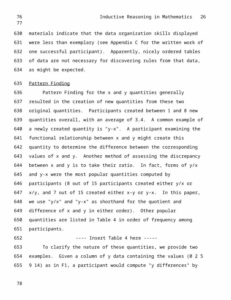
Pattern Finding for the x and y quantities generally resulted in the creation of new
quantities from these two original quantities. Participants created between 1 and 8 new
quantities overall, with an average of 3.4. A common example of a newly created quantity is
"y-x". A participant examining the functional relationship between x and y might create this
quantity to determine the difference between the corresponding values of x and y. Another
method of assessing the discrepancy between x and y is to take their ratio. In fact, forms of y/x
and y-x were the most popular quantities computed by participants (8 out of 15 participants
created either y/x or x/y, and 7 out of 15 created either x-y or y-x. In this paper, we use "y/x"
and "y-x" as shorthand for the quotient and difference of x and y in either order). Other popular
quantities are listed in Table 4 in order of frequency among participants.
---- Insert Table 4 here -----
To clarify the nature of these quantities, we provide two examples. Given a column of y
data containing the values (0 2 5 9 14) as in F1, a participant would compute "y differences" by
determining the difference between each pair of consecutive values in the column. Thus, 2 - 0
= 2; 5 - 2 = 3; 9 - 5 = 4; and 14 - 9 = 5. Therefore, the column for the quantity "y differences"
contains these values: (2 3 4 5). Given that same original column of y values, a participant
would compute "y factors" by listing any factor pairs that would produce the given y value.
6263
435
436
437
438
439
440
441
442
443
444
445
446
447
448
449
450
451
452
453
454
455
456
457
458
459
460
64

Inductive Reasoning in Mathematics 20
Thus, for y=9, 3*3 is a factor pair. For y=14, 2*7 is a factor pair. If there were a y=20, it
would have multiple factor pairs: 2*10, 4*5.
The quantities in Table 4 are all reasonably useful and informative to the participants.
We have provided some motivation for why "y/x" and "y-x" would be common quantities. The
other quantities in Table 4 are informative as well. Computing the "differences" within any
quantity is useful because it reveals how quickly the quantity is increasing or decreasing. The
quantity x-3 is informative in this particular problem because x-3 yields y for the first instance
in the problem: instance (3,0). Of course it is also the case that by computing x-3, one
translates the x values so that they begin at 0, which was aesthetically pleasing to some
participants. As for "y factors", it appears that this computation becomes salient whenever there
is a y value present which "lends itself" to factoring; in other words, when there is a y value
present for which the participant readily perceives a factorization, such as for y=14 or y=9.
This information can be very valuable if a pattern emerges from the factors of a sequence of y
values. Thus, participants found many ways to manipulate the original data in order to make
sense of it.
As important as PF is, successful and unsuccessful participants are not distinguished by
their use of PF. In fact, the basic PF processes used by both groups were virtually identical.
What does distinguish the two groups is the activity that follows the creation of a quantity.
Successful participants do not merely compute quantities; they analyze them. Having computed
some quantity q, the successful participant seeks to learn something about q. Is there anything
of interest or of value about this new quantity? Can it shed any light on the investigation
underway if it is probed a little? Successful participants use pattern recognition knowledge to
make good decisions about which intermediate quantities are worthwhile objects of pursuit.
We define the construct of "pursuit" to characterize this crucial process. The essence of pursuit
is to treat a newly created quantity as one would y, the original quantity. In other words,
subject the new quantity to analyses; take the differences between its values; form new
6566
461
462
463
464
465
466
467
468
469
470
471
472
473
474
475
476
477
478
479
480
481
482
483
484
485
486
67

Inductive Reasoning in Mathematics 21
quantities from it, etc. Each of the successful participants actively pursued intermediate
quantities. We return to this construct when we consider the strategies participants used to
succeed at this task. Now we turn to the third and final type of inductive activity observed in
the protocols.
Hypothesis Generation
Participants made use of two methods for generating hypothesis ideas. The first method
involves creating a hypothesis that works for a local (x,y) instance; the second, expressing an
observed pattern in terms of x. Every participant created "local hypotheses", in which a single
instance is used as the basis for creating a hypothesis (usually a simple, single-operator
hypothesis) that fits that instance. For example, for the instance (4,2), participants generally
produced the local hypotheses {x ÷ 2 = y} and {x - 2 = y}. Table 5 lists some common local
hypotheses. Although such local hypotheses rarely led directly to the answer for F1, they often
formed the basis of later, more advanced hypotheses. For example, the local hypotheses {x-3}
and {x/2} can both be considered as elements of the final solution: {(x/2)*(x-3)}. In a later
section we will characterize these particular local hypotheses in terms of pieces of a puzzle,
because they are the elements that must be put together in just the right way in order to reveal
the final function.
---- Insert Table 5 here -----
Once a participant generates a local hypothesis, the next step is to apply the hypothesis
to other instances to see if it approximates the desired y values. The basic types of local
hypotheses listed in Table 5 do not yield y for any instance other than the one for which they
were created. However, a determined participant could test the hypothesis on other instances to
examine the discrepancy between the outcome of the hypothesis and the desired y value.
Participant 11 applied this technique with the local hypothesis {x-3} by computing x-3 for
every instance possible. He then compared the resulting quantity to the desired y-values. This
was a helpful exercise because the relation between "x-3" and "y" (multiply by x, and divide by
6869
487
488
489
490
491
492
493
494
495
496
497
498
499
500
501
502
503
504
505
506
507
508
509
510
511
512
70

Inductive Reasoning in Mathematics 22
2) is less complicated than that between "x" and "y" (subtract 3, multiply by x, and divide by 2).
By examining the values of "x-3" in comparison to "y", this participant eventually succeeded at
discovering the correct solution (see the section on the Local Hypothesis Strategy.)
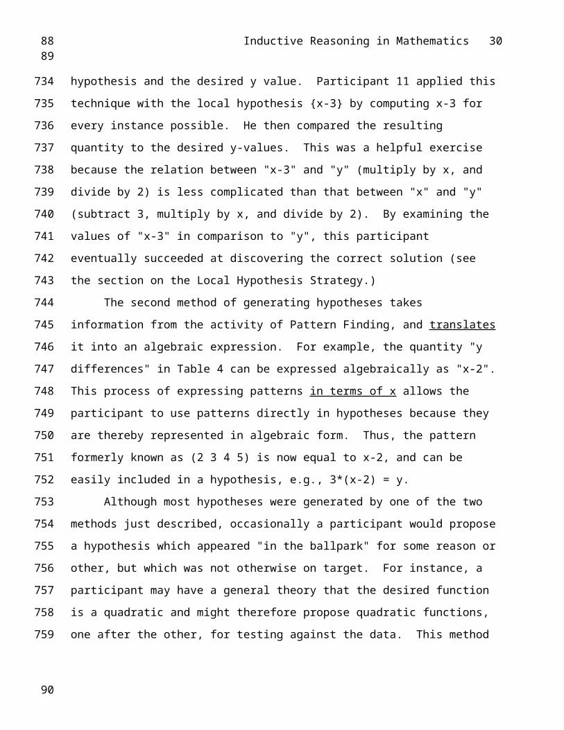
The second method of generating hypotheses takes information from the activity of
Pattern Finding, and translates it into an algebraic expression. For example, the quantity "y
differences" in Table 4 can be expressed algebraically as "x-2". This process of expressing
patterns in terms of x allows the participant to use patterns directly in hypotheses because they
are thereby represented in algebraic form. Thus, the pattern formerly known as (2 3 4 5) is now
equal to x-2, and can be easily included in a hypothesis, e.g., 3*(x-2) = y.
Although most hypotheses were generated by one of the two methods just described,
occasionally a participant would propose a hypothesis which appeared "in the ballpark" for
some reason or other, but which was not otherwise on target. For instance, a participant may
have a general theory that the desired function is a quadratic and might therefore propose
quadratic functions, one after the other, for testing against the data. This method was not
generally successful (indeed, no participant succeeded in solving the problem via this strategy),
which is not surprising given the relatively poor use of the data for guidance.
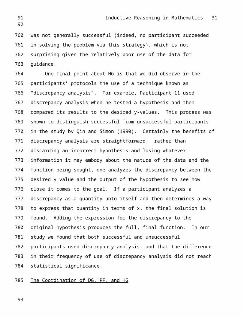
One final point about HG is that we did observe in the participants' protocols the use of
a technique known as "discrepancy analysis". For example, Participant 11 used discrepancy
analysis when he tested a hypothesis and then compared its results to the desired y-values. This
process was shown to distinguish successful from unsuccessful participants in the study by Qin
and Simon (1990). Certainly the benefits of discrepancy analysis are straightforward: rather
than discarding an incorrect hypothesis and losing whatever information it may embody about
the nature of the data and the function being sought, one analyzes the discrepancy between the
desired y value and the output of the hypothesis to see how close it comes to the goal. If a
participant analyzes a discrepancy as a quantity unto itself and then determines a way to express
that quantity in terms of x, the final solution is found. Adding the expression for the
7172
513
514
515
516
517
518
519
520
521
522
523
524
525
526
527
528
529
530
531
532
533
534
535
536
537
538
73

Inductive Reasoning in Mathematics 23
discrepancy to the original hypothesis produces the full, final function. In our study we found
that both successful and unsuccessful participants used discrepancy analysis, and that the
difference in their frequency of use of discrepancy analysis did not reach statistical significance.
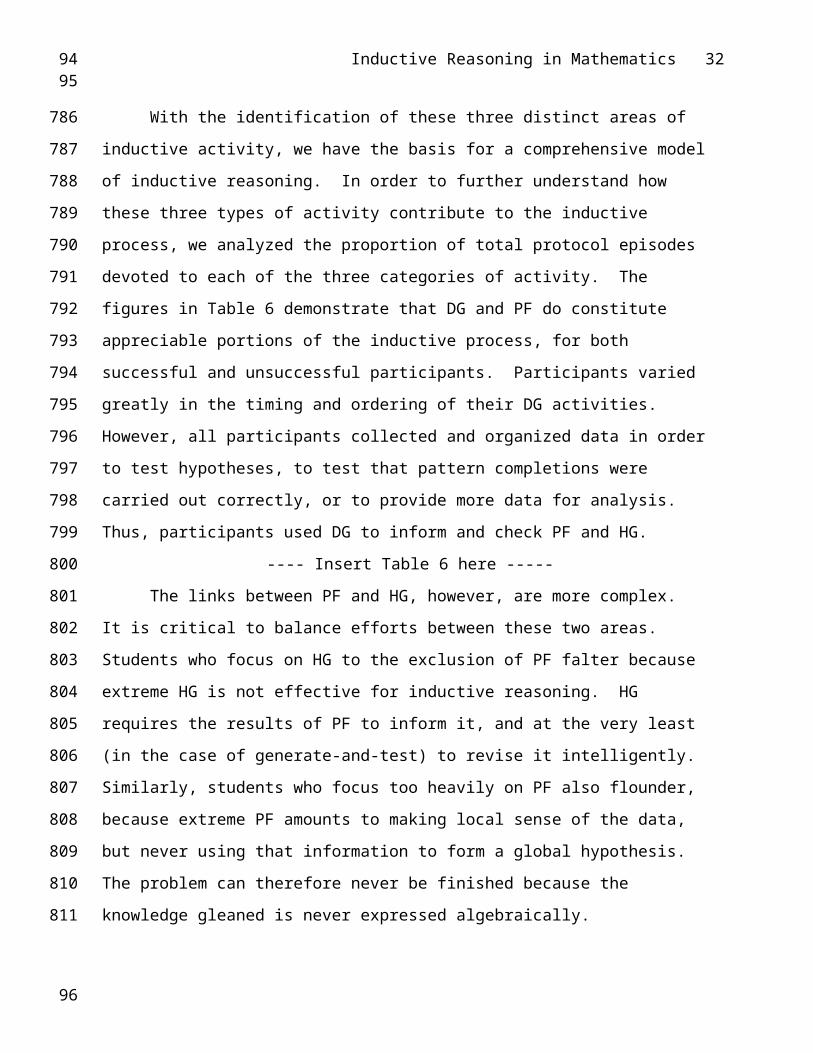
The Coordination of DG, PF, and HG
With the identification of these three distinct areas of inductive activity, we have the
basis for a comprehensive model of inductive reasoning. In order to further understand how
these three types of activity contribute to the inductive process, we analyzed the proportion of
total protocol episodes devoted to each of the three categories of activity. The figures in Table
6 demonstrate that DG and PF do constitute appreciable portions of the inductive process, for
both successful and unsuccessful participants. Participants varied greatly in the timing and
ordering of their DG activities. However, all participants collected and organized data in order
to test hypotheses, to test that pattern completions were carried out correctly, or to provide more
data for analysis. Thus, participants used DG to inform and check PF and HG.
---- Insert Table 6 here -----
The links between PF and HG, however, are more complex. It is critical to balance
efforts between these two areas. Students who focus on HG to the exclusion of PF falter
because extreme HG is not effective for inductive reasoning. HG requires the results of PF to
inform it, and at the very least (in the case of generate-and-test) to revise it intelligently.
Similarly, students who focus too heavily on PF also flounder, because extreme PF amounts to
making local sense of the data, but never using that information to form a global hypothesis.
The problem can therefore never be finished because the knowledge gleaned is never expressed
algebraically.
Based on these considerations, we hypothesized that successful participants would
allocate their effort evenly between PF and HG, while unsuccessful participants might allocate
their effort in a more lopsided way—either emphasizing PF at the expense of HG, or
emphasizing HG at the expense of PF. To test this hypothesis, we calculated a balance score
7475
539
540
541
542
543
544
545
546
547
548
549
550
551
552
553
554
555
556
557
558
559
560
561
562
563
564
76
Inductive Reasoning in Mathematics 24
for each participant, by taking the absolute value of the difference between the proportion of
episodes spent in PF and the proportion of episodes spent in HG. Low scores on this measure
reflect balanced allocation of effort across PF and HG, while high scores reflect lopsided
allocation.
As predicted, we found that successful participants tended to allocate their effort fairly
equally between PF and HG, while unsuccessful participants allocated their effort more
unequally (Means=21.2 successful, 39.5 unsuccessful, t(13)=2.17, p<.05, two-tailed). Among
the six unsuccessful participants, two spent more than half of their effort in HG, and three
participants spent more than half their effort in PF. Of the nine successful participants, only
two spent more than half their effort in either HG or PF.5 Thus, students who focused on one
process at the expense of the other tended to be unsuccessful. These students are reminiscent of
novice problem-solvers who repeatedly employed an unsuccessful problem-solving procedure
in a study by Novick (1988). Presumably students perseverate at these unsuccessful strategies
either because they do not know any other strategies to employ, or because they do not have the
necessary information with which to employ any other strategies. In contrast, successful
participants do not perseverate in a single activity, but achieve a kind of ideal: a balance of PF
and HG. We turn now to an analysis of these successful participants' solution strategies.
Observed Paths to Success
A total of three different paths to solution for F1 and F2 were employed by participants
in this study. We discuss them in order of increasing prevalence. Note that the use of the term
"strategy" does not necessarily imply here an explicit choice among options.
Recursive Strategy
The least common solution strategy was the Recursive strategy, for which participants
translated a method for computing y-values recursively into the correct closed-form function
hypothesis. The y-values for F1 (0, 2, 5, 9, 14, as listed in Figure 4) can be generated using a
very simple recursive method. Observe that the difference between the first two y-values listed
7778
565
566
567
568
569
570
571
572
573
574
575
576
577
578
579
580
581
582
583
584
585
586
587
588
589
590
79

Inductive Reasoning in Mathematics 25
(0 and 2) is 2; the difference between the next pair (2 and 5) is 3; and so on. We can thus
generate the value for y when x=8 by determining the difference between the y-values for x=6
and x=7, which is 14 minus 9, or 5. We increment this value by 1 to get 6, and add 6 to the y-
value for x=7 to get the y-value for x=8. Thus, when x=8, y must be 14+6=20. Similarly,
when x=9, y must be 20 + 7 = 27, and when x=10, y is 27 + 8 = 35.
This method of computing y-values is a recursive method because it relies on
knowledge of prior y-values to generate the current y-value. A closed-form method, on the
other hand, requires the current value of x, but not any previous values of y. Thus, with a
closed-form solution one can generate y-values for any x-value, no matter how high, without
resorting to calculating all of the y-values which preceded it.
The two participants who solved F1 via the Recursive strategy began by noting the
recursive formula just described. In fact, several participants discovered this piece of
knowledge (3 successful and 3 unsuccessful), but then also discovered that they could not use it
in the way they wished. The hypothesis that results from this recursive formula is: y = the
previous y + "x-2". To compute f(1000) using this rule, one needs to know the value for f(999).
Not even the most desperate participant attempted this extended calculation. Indeed, at this
point most participants abandoned this line of inquiry. Two participants, however, were able to
convert this recursive algorithm into a closed-form rule. These two noted that any given y-
value is the sum of all the y differences that went before it. In other words, the y-value when
x=7 is equal to 2+3+4+5 = 14. This sum series always begins at 2 and always ends at x-2
(again, recall the recursive formula). Thus, the problem is simply one of expressing the sum
from 2 to x-2. These two participants posed this simpler problem to themselves and were able
to retrieve (in one case) or to re-derive (in the other) the same formula that Gauss used for the
sum of the numbers from 1 to n: namely, n*(n+1)÷2 = the sum of the numbers from 1 to n. The
two participants applied this formula to the sum from 2 to x-2, and eventually arrived at an
algebraic equivalent of x*(x-3)÷2.6 These participants had specialized knowledge that helped
8081
591
592
593
594
595
596
597
598
599
600
601
602
603
604
605
606
607
608
609
610
611
612
613
614
615
616
82
Inductive Reasoning in Mathematics 26
them to succeed at this problem and that most likely set them apart from the unsuccessful
participants. Indeed, the math background of these two participants was high in relation to the
rest of the participants (they reported Math SAT scores of 780 and 710), indicating a likelihood
that they would have familiarity with this summation formula and have the algebraic skills to
deploy it.
Local Hypothesis Strategy
The Local Hypothesis strategy was used by two participants on F1 and by two
participants to solve F2. Thus, it was slightly more common than the Recursive strategy.
Every participant, successful or unsuccessful, engaged in the behavior of creating "local
hypotheses" to fit a solitary data instance; however, most participants did not rely solely on this
strategy to reach the final solution. An example of generating local hypotheses is the following.
Suppose that, given an x-value of 7 and a y-value of 14, we encounter a participant who
proposes {x + 7 = y} and {x * 2 = y} as local hypotheses which work for the particular values
of x=7 and y=14. This information, that adding 7 to 7 will result in the desired y-value of 14,
did not have to be represented in terms of x and y. The participant could merely record that
7+7=14, or that 2*7=14. In framing these relations in terms of x and y, however, the
participant is prepared to test whether this relation holds for other instances. It is this generic
capability to apply to other instances that establishes the observed relation as a local hypothesis.
Participant 11 (P11) exemplifies the strategy of producing local hypotheses in order to
generate a promising global hypothesis. When he closely examined the instance (7,14), he
already had in mind the notion that x-3 might be involved somewhere (from examining instance
(3,0)). Applying this "minus 3" idea to (7,14) he said:
X equals 7 gives us, Y equals 14. hm. Let's see, now if we think about that, 7
minus 3 equals 4, right? That's if there's minus 3, I might have to drop that
idea, but anyways, if there is, multiply that by, so you take, uh, X minus 3,
divided by, X times X minus 3, divided by 2? (emphasis added).
8384
617
618
619
620
621
622
623
624
625
626
627
628
629
630
631
632
633
634
635
636
637
638
639
640
641
642
85

Inductive Reasoning in Mathematics 27
The correct rule seems to appear almost effortlessly in a flash of insight. P11 knows
that he needs to use x (7), and that he might also use x-3 (4), to produce y (14). He recognizes
that 14 factors into 7*2 and he further recognizes that this can be achieved by multiplying 7 and
4, divided by 2. His solution comes largely from examination of this single instance, though it
was critical that his prior local hypothesis for instance (3,0) led to the investigation of x-3.
Consider the wide range of possibilities that might otherwise have been proposed!
Given the numbers 4 and 14, many avenues exist for relating the two: 4 plus 10 = 14; 4 times 2
plus 6 = 14; 4 plus 7 plus 3 = 14; 4 times 4 minus 2 = 14. Reasonable closed-form rules could
have been proposed to correspond with each of these relations: (x-3)+10 = y; (x-3)*2 + 6 = y;
(x-3) + x + 3 = y; (x-3)2 - 2 = y; respectively. P11 either avoided considering all these
possibilities, or he discarded them instantly, without even having time to verbalize his
consideration of them. Why when there are so many equally likely possibilities does he
stumble directly onto the correct one? The answer lies in his immediate retrieval of the fact that
14 factors into 7 and 2, and his subsequent, probably automatic, retrieval of the fact that 2 is
half of 4. With these powerful facts already in mind, the solution that he proposed is
more attractive than any others expressly because with these facts, he can express every
necessary step in terms of x, without any need for further "adjustments" by addition or
subtraction. In short, he already has 4 expressed in terms of x: (x-3). But, as one of the factors
of 14, he needs 2 instead of 4. Thus, (x-3)÷2. The other factor, 7, is already set equal to x.
Thus, 14 = 7 * 2 = x * (x-3)÷2 = y.
With respect to P11's solution path, it is difficult to overstate the essential role played by
the accessibility of arithmetic facts. Without the speedy retrieval of the fact that 14=7*2, P11
might have encountered great difficulty in choosing between the many alternatives for relating
4 to 14. Had he chosen a different relation, for example, 14 = 4*4 - 2, then his resulting full
formula, y = (x-3)2 - 2, would not have held for other instances, and he may never have found
his way back to the correct relation that he did, in fact, discover.
8687
643
644
645
646
647
648
649
650
651
652
653
654
655
656
657
658
659
660
661
662
663
664
665
666
667
668
88

Inductive Reasoning in Mathematics 28
Participant 15 had to work a little bit harder to produce his Local Hypothesis success
story. He actually collected Instance 100: (100, 4850). He was in the habit of factoring the y-
values for the instances he collected, and did so with this one as well. He broke 4850 down into
its prime factors: 2, 5, 5, 97. He then noticed that 97 just so happened to be 100 minus 3 (thus,
x-3), so he combined the remaining factors to see how he might also express them in terms of x.
Note that not just any participant would have succeeded with this information. This participant
is special, as are all the successful participants, in that he perseveres in attempting to express
relations in terms of x. He computes 2*5*5 = 50 and notes that 50 is half of 100; thus, x÷2. He
combines these expressions together, and voila: (x-3)*(x÷2), he has the answer.
Like the participants who succeeded via the Recursive strategy, the Local Hypothesis
participants also drew on particular background knowledge. However, unlike the Recursive
strategy, the knowledge required for the Local Hypothesis strategy is available to the general
population: the participants simply required knowledge of arithmetic facts (e.g., 97=100-3) and
factors (e.g., 14=7*2; 2=4÷2; 4850=97*5*2*2). What may differ between the participants who
succeeded via this strategy and others is the swiftness of their access to these facts. Given the
speed of certain decisions, it appears that their access to these facts may even have been
automatic in certain cases. Thus, speed of access to and accurate retrieval and computation of
number facts may have set these participants apart from the others.
Pursuit Strategy
By far, the most common strategy was to reduce the problem to a quantity with an easily
recognizable pattern. We call this the Pursuit strategy because it required that the participant
pursue a line of inquiry through several steps: 1) identification of a pattern in a quantity q, 2)
pursuit of q as a subgoal to understanding y, 3) expression of q in terms of x, 4) combination of
expressions into a global formula. For F1, the specifics are as follows. In the course of
standard Pattern Finding procedures, the participant looks for a number to answer the query, "x
times what equals y?". If the participant answers this question for enough instances, then she
8990
669
670
671
672
673
674
675
676
677
678
679
680
681
682
683
684
685
686
687
688
689
690
691
692
693
694
91

Inductive Reasoning in Mathematics 29
may be able to detect the fact that this quantity (q) increases by 1/2 with each increase in the
value of x. Having identified this pattern, the participant must make the decision whether or
not to pursue this line of inquiry further. If she decides to do so, the next step is to try to
understand the relationship between x and this new quantity q. Ideally, this attempt will
eventually result in the discovery of an algebraic expression which concretely specifies the
relation between x and q (i.e., (x-3)/2 = q). With such an expression in hand, the participant
now has the answer to the question "x times what equals y?", and can thus multiply by x to
complete the full formula: x*(x-3)/2 = y.
Five of the 9 successful participants on F1 employed this strategy, as did 13 of the 15
successful participants on F2, for a total of 18 out of 24 successes (75%), or 18 out of a total of
32 attempts (56%). Because it was the most common strategy, we provide a walk-through
example of this strategy, with highlights from one successful participant's protocol.
One Student's Solution to F1. What follows is a detailed examination of the critical steps
taken by one successful participant, "Ace". (The full text of Ace's verbal protocol, divided into
segments by carriage returns, appears in Appendix B. His written work appears in Appendix
C.) Ace does not begin by generating instances in any regular sequence. He collects them in
the order shown in Table 7.
---- Insert Table 7 here -----
Ace reorganizes this data before collecting x=6, so that the smaller x values (3, 4, 5) are
sequential, and then collects x=6 and x=7 and records them into a table like that seen in Figure
5.1. Figure 5 displays an overview of Ace's solution path from this point forward. Each step is
numbered (step numbers are circled) and outlined by a box. Where one quantity has been
computed in two different steps, inner boxes are used to denote the separate steps.
1. After some initial struggling (see protocol, Appendix B, lines 1-107), Ace
reorganizes the data so that it looks like the table seen in Figure 5.1.
---- Insert Figure 5 here -----
9293
695
696
697
698
699
700
701
702
703
704
705
706
707
708
709
710
711
712
713
714
715
716
717
718
719
720
94
Inductive Reasoning in Mathematics 30
2. Ace then computes the differences between the successive values of y (lines 108-
112):
" 0 to 2, is jump of 2,
2 to 5, jump of 3,
5 to 9, jump of 4,
9 to 14 is a jump of 5"
3. In examining these "y differences", Ace notices a relation between the column of x
values and the y differences (lines 116-118):
"X, .... X minus 2
is the increment of that jump.
from the number before."
The formula "x-2" characterizes the increment from one y-value to the next. Thus,
when x equals 6, x-2 = 4, which is indeed the difference between the corresponding y-value of
9 and the previous y-value of 5.
4. Using this recursive rule (computationally equivalent to yn = yn-1 + (xn - 2)) Ace
extrapolates to the instances where x=8 and x=9, and finally confirms the formula by producing
from it the correct y-value to correspond with x=10 (an instance he had already collected) (lines
121-130).
" X minus 2 is the increment
would be ...6 ...8
make it 20
so there's 9
make it 27
there's 10
you make 35.
figured that out."
9596
721
722
723
724
725
726
727
728
729
730
731
732
733
734
735
736
737
738
739
740
741
742
743
744
745
746
97
Inductive Reasoning in Mathematics 31
5. Ace realizes the limitations of his recursive formula. In order to find the value of
this function when x=1000, he would need to know the value of the function when x=999, and
so on (lines 131-150). He thus tries to find a way to predict y from x that does not require
knowledge of the previous y value (lines 151-162). (This is the point at which the Recursive
strategy diverges.) He is searching for a relation between x and y that remains true for several
instances. He notes that for the instances 5, 7, and 9, x can be multiplied by an integer to
produce the appropriate value of y (lines 163-165).
" 7 times 2 is 14.
9 times 3 is 27
5 times 1 is 5."
6. Ace notices that the quantity being multiplied (1, 2, 3), called q here, is increasing by
one. (He tests this with the pair (11,14).) However, he is only looking at every other x-value
(5, 7, 9, 11). Given this information, he guesses that q when x = 8 might be 2.5, the number
exactly between the values of q for 7 and 9 (lines 179-185). After testing that 8 times 2.5 does
equal the desired y-value of 20, Ace also notes that q=.5 works when x = 4 (lines 179-200).
" 8 times 2.5,
what's that equal?...
yeah that's it. . . . .
yeah, because 4 times .5 is 2"
The value q that Ace has discovered is actually equal to y/x. Use of this new quantity is a
critical step in the solution.
7. Having written down instances of this intermediate quantity q, Ace notices that they
increase by .5 with each increase of 1 in the value of x (lines 202-211).
" Y equals X times .5 for 4
Y equals X times 1 for 5
9899
747
748
749
750
751
752
753
754
755
756
757
758
759
760
761
762
763
764
765
766
767
768
769
770
771
100
Inductive Reasoning in Mathematics 32
and goes up by .5 each time. . . .
after 3 it goes up by .5 each time."
8. Ace now tries to find a relation that will "generically" specify how q increases by .5
with each increase of x (lines 218-235):
"trying to see
how you move the .5 up every time, generically....
I can't figure out a way to make it go up with the
X.
Y equals .... X times,
how do I get that .5
would be .... 4 minus 3"
The relation that Ace discovers between x and q ("would be ... 4 minus 3") is actually a
relation between x and the numerator of q, which we call q2. The value of q for x=4 is .5, or
1/2. Subtracting 3 from x we get 4 - 3 = 1, which is q2: the numerator of 1/2.
9. Ace examines another instance (x=5) and determines that the relation between x-3
and q2 continues to hold. For this instance, he goes a step further, and divides the numerator by
2 to get the actual q value of 1 (lines 237-241):
" 5 minus 3 divided by 2
get us the 1
so that would be
X minus 3 divided by 2"
Ace has taken the crucial step at this point of expressing in terms of x the relationship
between the quantities x and q that he has found to hold for the single instance x=5. This
general expression (x-3)÷2 will allow him to apply his new discovery to many other instances.
He tests this new formula with other instances (lines 242-246):
101102
772
773
774
775
776
777
778
779
780
781
782
783
784
785
786
787
788
789
790
791
792
793
794
795
796
103

Inductive Reasoning in Mathematics 33
" try 4 minus 3 divided by 2
that's... .5
try 8 minus 3 divided by 2
that equals the 2.5 that we need"
10. Finally satisfied that his partial formula (x-3)÷2 for yielding q is accurate, Ace
multiplies this partial formula by x to produce a full hypothesis (lines 247-250):
" so we have
Y equals X times
X minus 3
divided by 2."
Ace's solution can be summarized as follows: find for several instances the values that,
when multiplied by x, yield y (step 5, Figure 5). We call these new values q. Look for a
pattern within q and discover that q increases by 1/2 for each increment of 1 in x (step 7, Figure
5). Having discovered a pattern that holds for all values of x, aim to express q solely in terms
of x. In this way the new quantity is viewed as something to be investigated in its own right, or
to be pursued. The original goal was to express y in terms of x. A subgoal has now been
established to express q in terms of x. Pursue this subgoal by looking for patterns in (x,q)
instances. Ace pursues a further subgoal (step 8, Figure 5) by determining the relationship
between x and q2, the numerator of q. Having determined this relationship, he returns to the
prior subgoal of expressing the pattern in q in terms of x (i.e., (x-3)/2 = q) (step 9, Figure 5).
Recall that q was created because it could be multiplied by x to produce y. Thus, we multiply
the formula for q by x, and thereby produce a full formula for expressing y in terms of x (step
10, Figure 5).
In focusing on the relation between x and certain intermediate quantities related to y
(i.e., q and q2), Ace reduced the complexity of the problem he was solving: the relation
between "x" and "y/x" (subtract 3, and divide by 2) is less complicated than that between "x"
104105
797
798
799
800
801
802
803
804
805
806
807
808
809
810
811
812
813
814
815
816
817
818
819
820
821
822
106

Inductive Reasoning in Mathematics 34
and "y" (subtract 3, multiply by x, and divide by 2); and the relationship between x and q2
(subtract 3) is less complicated than that between x and q (subtract 3, and divide by 2). In fact,
Ace reduced the problem to such an extent that he determined the nature of a one-operator
relationship between x and another variable before he began to build back up to the full
hypothesis. It is useful to note here that Ace went beyond reducing the problem to one of a
linear relationship between x and another variable (which is the nature of the relationship
between x and q). F1 is a quadratic function, whereas q is a linear function of x (albeit a non-
prototypical one: (x-3)/2). Discovery of this linear relation would have been sufficient cause
for the BACON model to finish this problem. However, Ace's pursuit of the relation between q
and x (which is linear, but encompasses two operators) led to examination of the relationship
between x and the numerator of q (which is linear and has only one operator). Thus, the virtue
of pursuing intermediate quantities, like q and q2, is not specifically about reducing a quadratic
function to a linear one, but more generally about reducing the complexity of the problem to the
point where a pattern becomes recognizable and is simple enough to be readily expressed in
terms of x.
The Importance of Pursuit
Pursuit encompasses the following four activities. 1) Detect a pattern in a quantity q.
Decide that this pattern is worth pursuing. 2) Investigate the quantity q as you would y,
applying DG, PF, and HG tools. 3) Express q in terms of x. 4) Build on the algebraic
expression for q to propose a full hypothesis. Note that step 2 lends itself to recursion. In other
words, in the process of investigating q, the participant may happen upon an additional
quantity, say q2, that further simplifies the problem and that itself then merits pursuit (e.g., in
Ace's solution path, the numerator of the quantity y/x). This q2 would thus be expressed in
terms of x (just as Ace found the expression x-3 was equal to the numerator of y/x) as a
stepping stone to expressing q in terms of x. Expressing q in terms of x would, in turn, be a
stepping stone to expressing the full rule in terms of x. Successful participants did all of these
107108
823
824
825
826
827
828
829
830
831
832
833
834
835
836
837
838
839
840
841
842
843
844
845
846
847
848
109
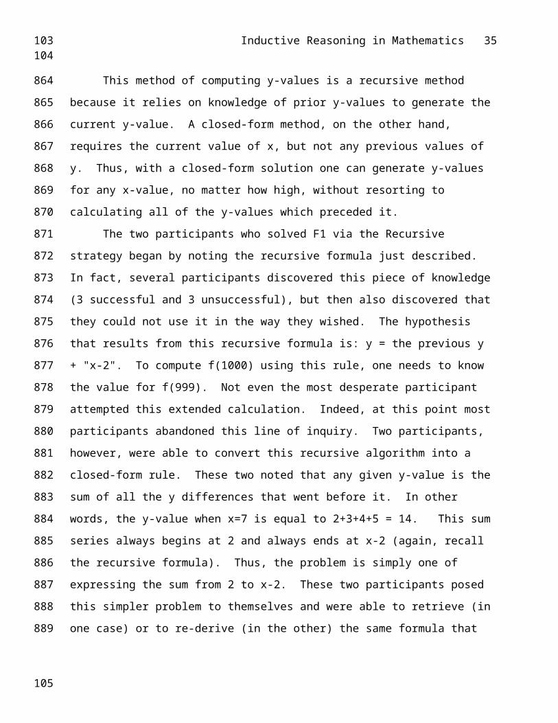
Inductive Reasoning in Mathematics 35
steps of Pursuit. Unsuccessful participants who took the first steps of the Pursuit strategy did
not see it through all of these steps. In this section we discuss how unsuccessful participants
failed in their Pursuit.
The Pursuit strategy for F1 involved the quantity q=y/x. Ten participants created this
quantity: 6 successful and 4 unsuccessful. (Table 8 lists the number of unsuccessful and
successful participants who made it to each step of the Pursuit process. Also included are the p-
values for whether or not the difference between the number of unsuccessful and the number of
successful participants reaching each step is statistically significant.) Nine of these participants
computed q for enough instances to distinguish a linear pattern in the quantity. The one
participant who did not was unsuccessful. Eight participants computed q for instances that were
equidistant from one another, and which therefore facilitated the detection of the linear pattern
in q. The participants who did not were unsuccessful.
In order to look for a pattern within q, or to produce any new quantities deriving from q,
a participant has to regard q as a new problem unto itself: a new "y" to subject to analysis with
all the tools in their inductive, pattern-finding toolbox. The heuristic of investigating and
analyzing a newly created quantity in its own right is the cornerstone of Pursuit. Ace pursued
q. He: 1) detected and investigated a pattern in q which eventually allowed him to 2) express q
solely in terms of x. Of the eight participants who computed q for enough instances in F1, only
6 of them detected the pattern in q that Ace did (Figure 5, step 7).7 Of the two participants who
did not detect this pattern, one was unsuccessful, and one eventually went on to solve the
problem via the Recursive strategy.
Finally, q cannot contribute to a participants' final solution unless it is expressible solely
in terms of x and can thereby be used as part of a formal algebraic formula. Of the 6
participants remaining in the Pursuit game at this point, only one did not attempt to express that
pattern in terms of x. This participant was unsuccessful. All 5 remaining participants did
110111
849
850
851
852
853
854
855
856
857
858
859
860
861
862
863
864
865
866
867
868
869
870
871
872
873
112

Inductive Reasoning in Mathematics 36
attempt and succeed at expressing this pattern in terms of x, and from there proceeded to solve
the problem.
---- Insert Table 8 here -----
Thus, at each step of the way, unsuccessful participants could and did abandon the
Pursuit strategy. In fact, every unsuccessful participant failed to persevere to the point of even
expressing q in terms of x, and did not even encounter the problem of constructing a final
hypothesis based on the algebraic expression for q.
Puzzle Pieces and Expression in Terms of X
The final step of Pursuit is to build a full hypothesis based on the fruits of one's prior
investigations. These algebraic expressions of patterns are like puzzle pieces: each must be fit
into the final formula in just the right way in order to produce the final product. The algebraic
formula that expresses q in terms of x, namely, q = (x-3)/2, is composed of two puzzle pieces
that have been pieced together. Recall how Ace constructed his final hypothesis one piece at a
time. He first reduced the problem to the discovery of the relation between x and q, and thus
introduced the notion that "*x" would be a component of the final function (because x * q
would equal y). He then discovered the relation between x and the numerator of q: "x-3".
Finally he included the component of dividing x-3 by 2, and, in combining all these pieces
together: "*x", "x-3", and "÷2", he produced his final hypothesis. These individual components
of F1 could be thought of as puzzle pieces that need to be fit together to construct the correct
rule.
Could it be that one or another of these pieces was particularly elusive to the
unsuccessful participants? Or was it the composition of the pieces that posed the real
challenge? For each unsuccessful participant, we coded whether each of these three pieces of
the F1 "puzzle" or any of their two-piece combinations were considered at any point during the
protocol (see Table 9). All but the "x-3" and the "x*" puzzle pieces reveal statistically
significant differences between successful and unsuccessful participants. Thus, unsuccessful
113114
874
875
876
877
878
879
880
881
882
883
884
885
886
887
888
889
890
891
892
893
894
895
896
897
898
899
115
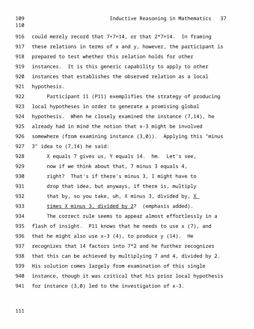
Inductive Reasoning in Mathematics 37
participants did not discover individual necessary components of the function. This result
leaves open the possibility that unsuccessful participants are as capable as successful
participants at recombining the puzzle piece elements to form the final function, if only they
have these elements on hand. Achieving these puzzle pieces, of course, requires expressing a
quantity in terms of x.
---- Insert Table 9 here -----
As seen in Table 8, expressing a pattern in terms of x seems to have been a major
stumbling block for unsuccessful participants. It is a step of Pursuit that no unsuccessful
participant completed. Furthermore, expressing a pattern in terms of x is the process by which
participants create puzzle pieces for fitting the final hypothesis together. Thus, it is not terribly
surprising that Table 9 shows that unsuccessful participants also had difficulty with discovering
the correct puzzle pieces.
How did successful participants express patterns in terms of x? Ace provides an
example in his step 9. Here is an example from another successful participant:
P7: "let's see how can we relate the number, the initial number to the
denominator, ... 8 goes to 5, that's minus 3, 10 goes to 7, that's minus 3, ...
alright, so maybe the denominator is [x] minus 3." (lines 735-750; note: this
participant was trying to express x/y, the reciprocal of q.)
By contrast, here is the excerpt from the protocol of the one unsuccessful participant
who did get as far as detecting the pattern in q, but who did not succeed in expressing q in terms
of x. This excerpt begins with the participant listing the values of (y-x)/x for instances 10, 9, 8,
7, and 6, respectively. (This participant was trying to express (y-x)/x, rather than y/x.):
P8: 2.5, 2, 1.5, 1, .5, um, .5 um, x plus .5x, x plus x, x plus 1.5x, x um, so if x
every time, add .5, x, plus 3, times, x plus, 3, 3x, um, 1.0x, um, x plus .5x, x
plus 1.0x, y, um, y, y plus 3?, y, y minus, divided by 3?, um, 6 plus 3 is 9, x
116117
900
901
902
903
904
905
906
907
908
909
910
911
912
913
914
915
916
917
918
919
920
921
922
923
924
118

Inductive Reasoning in Mathematics 38
plus, 7 plus 7 is 14, is 2, 2.5, 1.5, um, x plus .5, x, 1, 1.5, x plus 0x?, x plus
negative .5x....
Note that although P8 detects the pattern that (y-x)/x is increasing by .5, she does not
attempt to express the sequence of numbers .5, 1, 1.5, 2, 2.5 in terms of x (which would result
in the expression (x-5)/2)8, but instead simply inserts these y-derived values into instance-
specific formulas: for Instance 6: x + .5x = y, for Instance 7: x + 1x = y, etc. Without a general
characterization of the values .5, 1, 1.5, 2, 2.5 to insert into these instance-specific formulas,
she cannot move closer to her goal of finding a general hypothesis. She soon returns to
expressing these instance-specific formulas in their original, number-specific forms: 6+3 = 9,
7+7 = 14, only to return again to the futile effort of expressing these individual formulas in
terms of x: for Instances 5 and 6: "x plus 0x?, x plus negative .5x."
Summary of Successful Strategies
The three strategies to success, Recursive, Local Hypothesis, and Pursuit, share certain
elements. Perseverance and the goal to express relations in terms of x are essential to all.
Further, each strategy relied on mathematical background knowledge, particularly pattern
recognition knowledge for relations between particular numbers. In our computer model of
inductive problem solving, we have tried to capture the essential elements of the successful
Pursuit strategy.
The PURSUIT Model
Based on the protocol data described above, we developed a cognitive model of
participants' performance, in order to further articulate our theory of inductive reasoning. We
chose to simulate the Pursuit strategy because it was the strategy used most often. Our theory
of the cognitive processes involved in Pursuit includes the following activities: (1) Detect
patterns by examining the data, (2) Create new quantities, (3) Express patterns in terms of x, (4)
Construct hypotheses, and (5) Test hypotheses. We developed a production system model
called PURSUIT, based in ACT (Anderson, 1993), to simulate these processes. Data collection
119120
925
926
927
928
929
930
931
932
933
934
935
936
937
938
939
940
941
942
943
944
945
946
947
948
949
950
121

Inductive Reasoning in Mathematics 39
and organization strategies are not addressed in the PURSUIT model (the data is already
"collected" and organized into an ordered table when PURSUIT begins the problem.)
In the PURSUIT model, quantities are represented as lists of values, and hypotheses store
a conjectured algebraic relationship between two quantities. The model starts with the
quantities x and y, corresponding to the list of x and y values given in the problem, and without
any hypotheses. During problem solving, the PURSUIT model creates new intermediate
quantities, like q and q2 in the example of Ace above, and generates new hypotheses.
The procedural knowledge in PURSUIT is represented in if-then production rules. For
example, the following is an English version of PURSUIT's knowledge of how to find the
multiplicative relation between two quantities: "If the goal is to find a relationship between the
source quantity, S, and the pursuit quantity, P, Then for each instance of S and P find the value
you need to multiply S by to get P, and create a new quantity that contains these values." For a
complete list of the English versions of PURSUIT's productions, see Appendix D.
In the PURSUIT model, x is designated as the original "source" quantity from which we
want to be able to compute y, and y is designated as the original "pursuit" quantity, which we
want to be able to compute, given x. Before it pursues any quantity other than y, the PURSUIT
model establishes that said quantity is worthy of pursuit by assessing whether the quantity
contains a recognizable pattern. When the model encounters a quantity that does not contain a
pattern that it recognizes, the model returns to focusing on previous pursuit quantities.
Pattern Finding Productions
PURSUIT has productions for both Pattern Finding and Hypothesis Generation activities
(see Table 10). The PF activities observed in the protocols of all participants are encapsulated
in the following PURSUIT productions: Relate-by-addition, Relate-by-subtraction, Relate-by-
multiplication, Find-differences-within-quantity, Examine-numerator, and Recognize-pattern.
The "Relate-by" productions examine the arithmetical relations between the source quantity
(i.e., x) and the pursuit quantity (e.g., y). These productions can be thought of as a kind of
122123
951
952
953
954
955
956
957
958
959
960
961
962
963
964
965
966
967
968
969
970
971
972
973
974
975
976
124

Inductive Reasoning in Mathematics 40
discrepancy analysis (Qin & Simon, 1990), or as a way to compute the difference between a
pursuit quantity, such as y/x, and x itself when searching for a way to express a quantity in
terms of x. Thus, Relate-by-subtraction would compute the difference between the x-value and
y-value in each (x,y) pair. The Find-differences-within-quantity production creates the "y
differences" quantity that we encountered in Table 4 and in Ace's step 2, and the Examine-
numerator production allows the model to examine the top half of a series of fractions,
something which the human eye can do with relative ease. The ultimate goal of PF, of course,
is to actually detect a pattern. This crucial step is accomplished (or not) by the Recognize-
pattern production. This production is supplied with a small list of patterns which it recognizes
instantly: the counting numbers, the odd numbers, and the even numbers. With these PF
productions, the PURSUIT model can create all of the quantities created by participants on F1, as
listed in Table 4.
---- Insert Table 10 here -----
Hypothesis Generation Productions
PURSUIT's HG productions are: Express-in-terms-of-X, Unwind-subtraction, Unwind-
multiplication, Unwind-division, Test-hypothesis, and Finish. The most crucial of these HG
productions is Express-in-terms-of-X. This production fires whenever a relationship between
the source quantity (i.e., x) and the pursuit quantity, P, has been found which requires only the
adding, subtracting, multiplying, or dividing of some constant in order to produce P from x
(i.e., x - 3 = P). In other words, this production fires when the relationship being pursued is a
single-operator relationship. It is with this production that the process of building a hypothesis
arises from the fruits of Pattern Finding. Once an initial algebraic expression has been created
from this production, the other HG productions can fire. The "Unwind" productions reverse the
PF computations which produced the final pursuit quantity, recombining the puzzle pieces
found along the way so that the hypothesis will eventually yield the original pursuit quantity, y.
125126
977
978
979
980
981
982
983
984
985
986
987
988
989
990
991
992
993
994
995
996
997
998
999
1000
1001
127
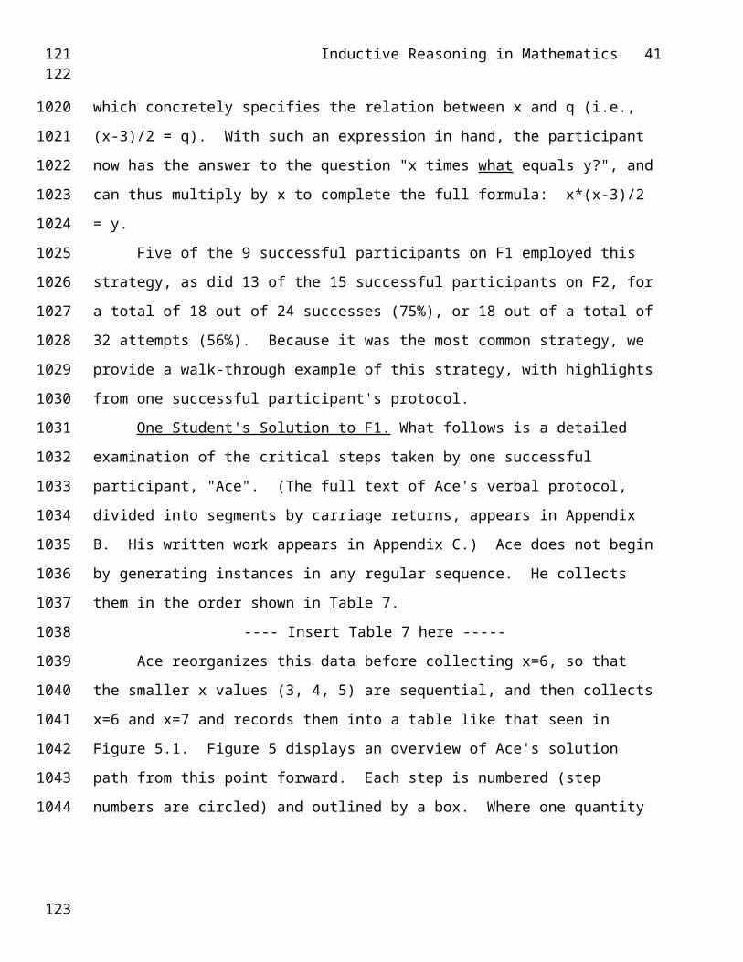
Inductive Reasoning in Mathematics 41
Finally, the Test-hypothesis and Finish productions test that the final hypothesis holds for
several instances and then declare the problem solved.
PURSUIT 's Successful Performance on F1
For F1, PURSUIT is provided with the quantities x (3 4 5 6 7) and y (0 2 5 9 14). Table
11 summarizes the sequence of productions used by the PURSUIT model to solve F1, as well as
the corresponding changes to the model's knowledge. A possible first step the model can take is
to fire the "Relate-by-multiplication" production. This production produces a new quantity that
we called q in Ace's protocol, but that we will refer to here as A = y/x to indicate how it relates
to x and y. In the second step (#2 in Table 11), the Recognize-pattern production examines A
to determine whether it matches any patterns in the model's repertoire of pattern recognition. If
the quantity matches a known pattern, it is designated worthy of further pursuit. It is at this
crucial point in the problem that the PURSUIT model uses its repertoire of pattern knowledge to
decide that the quantity A is worthy of further pursuit. In order for the model to make this
decision, as did the successful participants, we have included in its pattern recognition
repertoire the knowledge to recognize the pattern in A, which is that the quantity increases by
1/2 with each successive value. Thus, the Recognize-pattern production recognizes the pattern
in A and designates A for further pursuit.
In Step 3, the Examine-numerator production multiplies A by its constant denominator
so that the model may investigate the numerator alone (the quantity which we referred to as q2
in Ace's protocol, but which we refer to here as B). At this point (step 4), the model recognizes
a pattern in B: the values (0 1 2 3 4) match the production's template for the counting-numbers.
Thus, the quantity B, in y = x * B/2, is designated as the new Pursuit quantity. As such, the
model now begins to investigate ways in which the source quantity, x, might be related to this
new Pursuit quantity, B. The model succeeds in relating these two quantities by subtraction
(step 5) and the result is a constant difference of 3. At this point, the Express-in-terms-of-X
128129
1002
1003
1004
1005
1006
1007
1008
1009
1010
1011
1012
1013
1014
1015
1016
1017
1018
1019
1020
1021
1022
1023
1024
1025
1026
130

Inductive Reasoning in Mathematics 42
production fires because the source quantity x and the pursuit quantity P differ by only a
constant. The model thus produces its first algebraic expression: x-3=B.
A pursuit quantity, B, has now been expressed in terms of the source quantity, x. The
connection from x to y has been made. What remains is to reconstruct the steps taken to get to
B so that we may express y in terms of x. B was created by dividing the previous pursuit
quantity, A, by 2. The Unwind-multiplication production (step 7) reverses this step and divides
the new algebraic expression {x-3} by 2. The model now has an algebraic expression {(x-3)/2}
for the pursuit quantity A. A, however, was created to yield y when multiplied by x. Thus, the
Unwind-division production fires and multiplies by x our expression for A, thus creating a full
expression for y. Finally, the Test-hypothesis production fires and determines that this
algebraic expression for y does hold for several instances, and the Finish production fires,
declaring the problem solved.
---- Insert Table 11 here -----
We already noted the important role played by the Recognize-pattern production in this
solution. For this production to recognize the counting numbers (i.e., recognize any portion of
the sequence 1 2 3 4 5....) is not terribly controversial, as even the most rudimentary math
education allows for this competence. The ability to recognize differs-by-halves, however, is
more subtle, especially since participants' initial representations of the quantity A are generally
1, 1.5, 2, 2.5,... or 1, 11/2, 2, 21/2,..., rather than 1.0, 1.5, 2.0, 2.5,... or 2/2, 3/2, 4/2, 5/2,... .
Recall that some unsuccessful participants did have the data for y/x, yet they did not pursue this
useful quantity. Our theory is that the unsuccessful participants did not pursue y/x because they
did not recognize the pattern within it and therefore did not recognize the quantity as simpler
than y itself.9 Thus, they abandoned this path as not likely to be productive.
PURSUIT 's Unsuccessful Performance on F1
If the PURSUIT model has an appropriate and accurate decomposition of knowledge it
should be able to capture individual differences in participant performance. We demonstrate
131132
1027
1028
1029
1030
1031
1032
1033
1034
1035
1036
1037
1038
1039
1040
1041
1042
1043
1044
1045
1046
1047
1048
1049
1050
1051
1052
133

Inductive Reasoning in Mathematics 43
PURSUIT's accuracy by showing how the model captures the performance of unsuccessful
participants. To simulate unsuccessful performance on F1, the differs-by-halves pattern is
removed from the list of familiar patterns for the Recognize-pattern production. Impaired in
this way, the PURSUIT model computes several quantities that compare x and y, including
Relate-by-multiplication (which yields A=y/x), Relate-by-subtraction (which yields C=y-x),
and Find-differences-within-quantity (which yields D=y differences). One possible path is
shown in Table 12. The only one of these new quantities that is recognized by the Recognize-
pattern production is D, which has the values (2, 3, 4, 5): the counting numbers. The model
recognizes these y differences as a Pursuit quantity, and therefore may apply Find-differences-
within-quantity again, or Relate-by-subtraction, with x as the source quantity and D as the
pursuit quantity.
---- Insert Table 12 here -----
PURSUIT does apply Relate-by-subtraction (step 5 in Table 12) with the result that x and
D differ by a constant value of 2. At this point, the Express-in-terms-of-X production fires and
produces the algebraic expression that (x-2) = y differences. PURSUIT would now apply further
HG productions if any of them applied, but the within-quantity difference operation that
produced the y differences quantity is not reversible algebraically. Thus, PURSUIT reaches an
impasse.
Note that our successful participant Ace also reached this impasse. The steps taken by
the unsuccessful PURSUIT model are mirrored in Ace's steps 2 and 3. However, the only
formula that could arise out of this (x-2) = y differences expression is a recursive one:
f(x) = (x-2) + the previous y value.
This is not a closed-form algebraic function, and, like Ace and like most participants,
the PURSUIT model cannot produce a closed form solution from the recursive formula. When
participants, both successful and unsuccessful, arrived at this impasse (in total, six participants:
3 successful and 3 unsuccessful) they generally scrapped what they had found and began again
134135
1053
1054
1055
1056
1057
1058
1059
1060
1061
1062
1063
1064
1065
1066
1067
1068
1069
1070
1071
1072
1073
1074
1075
1076
1077
1078
136

Inductive Reasoning in Mathematics 44
with the original x and y (with the exception of the two participants who succeeded with the
Recursive strategy, as previously described).
Thus, the model arrives at an impasse when it attempts to solve F1 without the ability to
recognize the differs-by-halves pattern in y/x. As such, we do not need to assume that
unsuccessful participants are incapable of producing y/x in order to explain their failure at
discovering F1. This is an important point. Prior work in this domain (Huesmann & Cheng,
1973; Gerwin & Newsted, 1977) maintained that functions involving division pose particular
difficulty for students trying to induce them. Our model suggests that this difficulty is not due
to an inability to use or to conceive of using division, but rather to a failure to recognize when
division has led to a simplification of the problem. Quantities resulting from division often
involve fractions or decimals, rather than whole numbers, and such quantities may be difficult
to recognize as problem simplifications (see again footnote 9). Our data show that unsuccessful
participants did consider division and were capable of performing division, and these skills are
thus intact in the unsuccessful model. The thing that is impaired is the ability to recognize a
certain pattern. Note that the PURSUIT model's simulation of unsuccessful performance also
does not necessitate the removal of the fundamental idea of pursuing and analyzing a new
quantity just as if it were the original y quantity. It is knowing what to pursue that
differentiates the successful and unsuccessful outcomes. Indeed, our model indicates that
limited numerical pattern recognition knowledge is the critical distinguishing feature of
unsuccessful performance.
PURSUIT 's Successful Performance on F2
Given that the PURSUIT model accounts for both successful and unsuccessful
performance on F1, can both these versions of the model also succeed at F2? It is a crucial test
for the validity of our model to determine whether it can account for the failure of unsuccessful
participants on F1 as well as their overwhelming success in finding F2. Fifteen of the 16
participants succeeded at finding F2; only one participant failed, and this one also failed at F1.
137138
1079
1080
1081
1082
1083
1084
1085
1086
1087
1088
1089
1090
1091
1092
1093
1094
1095
1096
1097
1098
1099
1100
1101
1102
1103
1104
139

Inductive Reasoning in Mathematics 45
Of those who succeeded on F2, 13 did so via the Pursuit strategy and calculation of y/x (the
other two, both of whom were successful on F1, succeeded via the Local Hypothesis strategy).
The PURSUIT model simulates this common Pursuit strategy for solving F2 via the computation
of y/x. Table 13 lists the productions that fire to solve F2.
---- Insert Table 13 here -----
For F2, PURSUIT is provided with the quantities x (1 2 3 4 5) and y (3 10 21 36 55). The
Relate-by-multiplication production fires first. This production produces the quantity A =y/x.
In step 2 the Recognize-pattern production examines A (3, 5, 7,...) and finds that it matches the
odd-numbers template. A is thus marked a Pursuit quantity and the model begins to investigate
patterns and relations between x and A. In the third step, the model relates x and A by addition,
so that the quantity B = A-x is created. Once again, the Recognize-pattern production fires, this
time recognizing the quantity B (2, 3, 4,... ) as matching the counting numbers. PURSUIT now
looks for a relation between x and the new pursuit quantity, B. The Relate-by-addition
production finds that the corresponding values for B and x differ by a constant value of 1. At
this point, Express-in-terms-of-X fires and produces the algebraic expression: x+1=B. To
reconstruct the steps taken to get to B, the Unwind-subtraction and Unwind-division
productions fire (steps 7 and 8). The resulting hypothesis is x*(2x+1) = y, and the problem has
been solved.
Although this solution path is very similar to the solution for F1, participants who used
this strategy successfully on F2 did not succeed in following the same strategy to solution for
F1. For the model, the only difference between successful and unsuccessful performance on F1
is the ability to detect the differs-by-halves pattern in y/x. For the solution to F2, this pattern
does not play a role, and so the full and the impaired versions of PURSUIT from F1 perform
identically to solve F2.
Model Summary
140141
1105
1106
1107
1108
1109
1110
1111
1112
1113
1114
1115
1116
1117
1118
1119
1120
1121
1122
1123
1124
1125
1126
1127
1128
1129
142

Inductive Reasoning in Mathematics 46
Thus, the PURSUIT model, endowed with Pattern Finding and Hypothesis Generating
productions, accounts for both successful and unsuccessful performance on F1, as well as
success on F2. One key finding is that the adjustment needed to produce success vs. failure on
F1 is not an adjustment of procedural knowledge. PURSUIT's model of unsuccessful
performance contains all the same productions as the successful model, just as the unsuccessful
participants in this study engaged in the same PF and HG behaviors as did the successful
participants. Instead, it is pattern recognition knowledge that differentiates the full and
impaired versions of the PURSUIT model.
The difference in declarative knowledge between the successful and impaired model
was a difference in the types of patterns that the model recognized. The successful version
recognizes that successive values of a particular quantity increase by one-half. It pursues the
quantity containing that pattern, and ultimately discovers the complete hypothesis. The
impaired version of the model does not recognize this pattern, and consequently does not pursue
the simpler quantity, and is unable to construct the final hypothesis. Thus, a small difference in
pattern finding accounts for the difference between success and failure on F1. In this way, the
model demonstrates that pattern finding plays an essential role in inductive reasoning.
Discussion
This study has revealed some crucial processes involved in inductive reasoning, a skill
which is required in both mathematics and science, and which plays a role in problem-solving
performance, learning, and the development of expertise (Holland, et. al., 1986; Pellegrino &
Glaser, 1982; Simon & Lea, 1974; Egan & Greeno, 1974; Chi, et. al., 1982). Indeed, inductive
learning methods aid the acquisition of problem-solving knowledge even in problem domains
that appear deductive on the surface (Johnson-Laird, 1983; Koedinger & Anderson, 1989,
1998). Furthermore, induction has recently been targeted as an important educational objective
in math education (NCTM, 1989; Serra, 1989); although a detailed understanding of the
cognitive processes that support inductive reasoning is still lacking. The current investigation
143144
1130
1131
1132
1133
1134
1135
1136
1137
1138
1139
1140
1141
1142
1143
1144
1145
1146
1147
1148
1149
1150
1151
1152
1153
1154
1155
145

Inductive Reasoning in Mathematics 47
was designed to advance our understanding of the cognitive skills required for inductive
reasoning in mathematics.
In this investigation, we assessed inductive reasoning using function-finding tasks.
These tasks are representative of inductive reasoning tasks in that they require several of the
processes identified by Klauer (1996) as central to inductive reasoning. Specifically, function-
finding tasks require detecting and characterizing both similarities and differences in the
relationships between successive pairs of numbers. The function-finding task is also
representative of inductive reasoning in mathematics, because the problem of finding functions
from data is fundamental to many areas of mathematics. Mathematicians and scientists use
function finding when searching for a rule or theory to describe a set of data. Function-finding
problems are also embedded in domains in which numbers do not appear on the surface (e.g.,
the geometry example in Figure 2), and can also arise to aide in the recall of formulas or
procedures (e.g., the combinatorics example in Table 3). Thus, function finding is important in
a wide variety of mathematical endeavors.
We wished to investigate the inductive reasoning processes used by non-expert but
intelligent problem solvers, so we chose undergraduate students as our participant population.
By presenting function-finding problems to intelligent novices -- non-experts who nevertheless
have the general strategies and knowledge to be successful in novel situations -- we attempted
to ensure that the reasoning processes we observed would indeed be inductive.
Empirical Summary
This study identified three basic activities involved in inductive reasoning that students
engage in to solve function-finding problems: Data Gathering, Pattern Finding, and Hypothesis
Generation. We identified Data Gathering as an important process that is more variable and
less structured than has been implied in the literature, and we demonstrated that successful and
unsuccessful students collect comparable data instances and organize data with comparable
skill. Nevertheless, in this study, Data Gathering did not differentiate successful from
146147
1156
1157
1158
1159
1160
1161
1162
1163
1164
1165
1166
1167
1168
1169
1170
1171
1172
1173
1174
1175
1176
1177
1178
1179
1180
1181
148
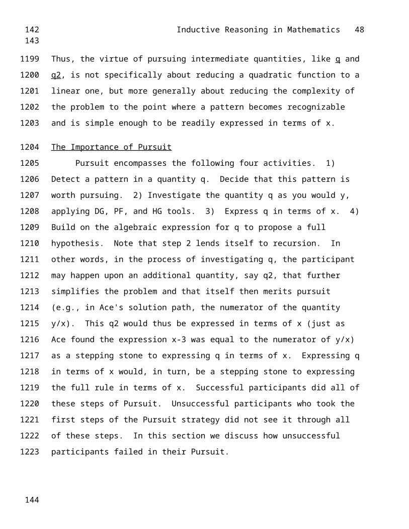
Inductive Reasoning in Mathematics 48
unsuccessful performance. Successful and unsuccessful students did differ in how they used
Pattern Finding and Hypothesis Generation. Students who did not succeed at solving the
problems tended to allocate the majority of their effort to either Pattern Finding or to
Hypothesis Generation, and did not use Pattern Finding to inform Hypothesis Generation or
vice versa. In contrast, successful students allocated their effort evenly across Pattern Finding
and Hypothesis Generation and integrated these two activities throughout the course of their
problem solving. This integration was apparent in all of the successful protocols, regardless of
the particular solution path followed.
Three different solution paths were followed by successful students in this study: the
Local Hypothesis solution path, the Recursive solution path, and the Pursuit solution path. In
both the Recursive and the Local Hypothesis paths, students translated observed patterns and
relationships into algebraic expressions that eventually produced the final hypothesis. In the
Pursuit path, which is instantiated in our cognitive model, students detected patterns and
expressed them generally, in terms of x, and then constructed the final hypothesis by combining
smaller hypothesis pieces together.
The Pursuit strategy was the most common strategy used for both of the problems in this
study. The frequent use of this strategy suggests that the activity of pursuit is often necessary in
inductive reasoning. Indeed, inductive problem solving is seldom accomplished in a single
flash of insight, especially when the rule to be discovered is complex. In the case of function-
finding for undergraduates, quadratic polynomial rules were sufficiently complex that students
did not solve the problems in a single step. In such situations it becomes necessary to find ways
to simplify the problem. In the Pursuit strategy, students simplify problems by identifying and
pursuing quantities that are less complex than the original y.
It is important to note here that the solution paths followed by undergraduates are not
generally optimal in terms of reaching a solution quickly and efficiently. However, our purpose
in this study was not to examine mature, optimal strategies for solving function-finding
149150
1182
1183
1184
1185
1186
1187
1188
1189
1190
1191
1192
1193
1194
1195
1196
1197
1198
1199
1200
1201
1202
1203
1204
1205
1206
1207
151

Inductive Reasoning in Mathematics 49
problems. Instead, we chose function finding as a representative inductive reasoning and
mathematics task, and we chose to examine and model the problem-solving activities of non-
experts because we wanted to tap inductive processes - not proven, deductive strategies. It is
easy enough to solve a polynomial function-finding problem in a non-inductive way.10 If we
had examined expert performance on function-finding problems they might well have used
formal, non-inductive strategies, and we would not have any inductive processes to study or to
model. We purposely examined the activities of bright students in a relatively unfamiliar
inductive domain so that we could examine how people without domain-specific strategies
would approach the problems. It is because we attempted to identify relatively domain-general
strategies that these results are applicable to more areas of mathematics than just function-
finding problems.
Model Summary
The PURSUIT cognitive model instantiates the Pursuit solution path. As such, it
demonstrates that induction of the final hypothesis is not accomplished all at once. Instead, the
hypothesis is constructed step by step, out of what we have called puzzle pieces. Each separate
algebraic piece is expressed in terms of x and then incorporated into the final solution. The
model's highlighting of this process is an important contribution to our understanding of
"system construction" inductive reasoning problems (see Klauer, 1996). It would be incredibly
difficult to recognize the rule for any complex set of data without first decomposing the
problem into simpler components. People do not typically look at the data X 3 4 5 6 7Y 0 2 5 9 14 and simply produce the full hypothesis: y = x(x-3)/2. Not even our
fastest successful participant approached such sophistication. Accordingly, the PURSUIT model
must engage in three full cycles of relating variables and recognizing patterns before it can
compose the pieces required to solve this problem. For more simple functions, however, the
story is quite different. People can and do look at the data X 3 4 5 6 7Y 0 1 2 3 4 and very
quickly produce the hypothesis that y = x-3 (at least in this participant population). Similarly,
152153
1208
1209
1210
1211
1212
1213
1214
1215
1216
1217
1218
1219
1220
1221
1222
1223
1224
1225
1226
1227
1228
1229
1230
1231
1232
1233
154

Inductive Reasoning in Mathematics 50
our model requires only two productions to solve this single-operator problem. Our model, like
our participants, does not solve F1 (the more difficult function) by inspection, but breaks the
problem into subproblems and then builds back up to the full hypothesis. Thus, the PURSUIT
model emphasizes the importance of reducing a complex problem to a set of simpler problems.
Note that for both the students and the model, the simpler subproblems seem to be
inducible almost by inspection. Note also that all of these subproblems require only single-
operator relations (e.g., x-3). Indeed, in our model, the "Express-in-terms-of-x" production
fires only for single-operator relations. Although this result does not mean that people cannot
induce relations that involve more than one operation, it is certainly suggestive.
One final contribution of our model is that it identifies a critical difference between the
successful inductive reasoning of our successful participants and the failed attempts of the
unsuccessful inducers. Both the successful and the impaired versions of our cognitive model
have the necessary procedures to carry out the Pursuit strategy. Both are equipped to recognize
patterns and to pursue promising quantities. However, the capacity of each model to recognize
patterns is dependent on the repertoire of patterns that we enabled the model to recognize. The
successful version is provided with a larger repertoire of number patterns than the impaired
version, and is thus capable of succeeding when the impaired model does not. This dependence
on pattern recognition enables the PURSUIT model, unlike prior models of discovery and
inductive reasoning (e.g., Qin & Simon, 1990; Huesmann & Cheng, 1973; Gerwin & Newsted,
1977) to account for the fact that the same students who failed at discovering one quadratic
function in this study succeeded at solving the other (for which the impaired model did have the
necessary pattern in its repertoire). Thus, the model mimics the performance of students who
succeed at solving problems that require patterns that they have in their repertoires, and fail at
solving problems that require patterns that they do not recognize.
The PURSUIT model instantiates the inductive, non-expert solution path most commonly
exhibited by participants in this study. In doing so, it highlights the importance to inductive
155156
1234
1235
1236
1237
1238
1239
1240
1241
1242
1243
1244
1245
1246
1247
1248
1249
1250
1251
1252
1253
1254
1255
1256
1257
1258
1259
157
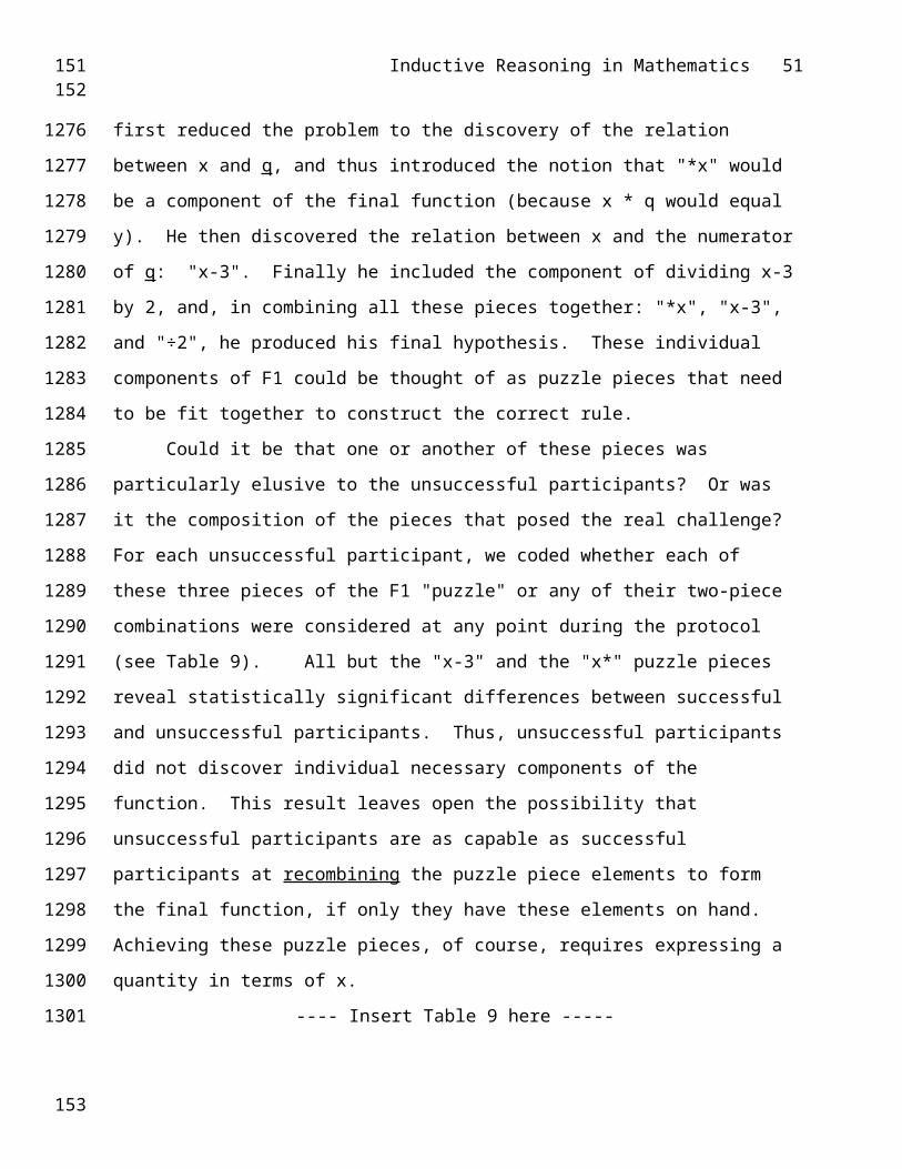
Inductive Reasoning in Mathematics 51
reasoning of pattern recognition knowledge as well as the importance of breaking problems
down into simpler, "inducible" components that require only one operation to be expressed
generally.
Importance of Pattern Recognition
Our model highlights the detection of patterns as crucial to inductive reasoning. Indeed,
the pursuit process, which simplifies complex problems, can only occur when pattern detection
skills are sufficient to identify quantities that are less complex than the original y. The process
of pursuit is thus dependent upon the student’s ability to recognize useful patterns and to
thereby make informed, intelligent pursuit decisions. If a student fails to recognize the pattern
in a useful quantity, that student may incorrectly conclude that the path represented by that
quantity is unproductive, and thus abandon that line of pursuit. Students who lack pattern
recognition knowledge are thus more likely to follow unproductive paths, or to abandon paths
that would ultimately be productive. In other words, it is not because students do not know to
look for patterns, but because they do not find any patterns that they fail at pursuit. We
conclude that the ability to recognize a repertoire of possible patterns (and not just the particular
pattern emphasized for the problem in this study) is crucial to inductive reasoning in
mathematics.
There is extensive support in the literature for the idea that pattern recognition is
important in problem solving. Many studies have shown, for example, that pattern recognition
knowledge is a major difference between experts and novices (e.g., Chase & Simon, 1973;
Koedinger & Anderson, 1990; Chi, et. al., 1982). Such pattern recognition necessarily requires
domain knowledge, which experts have in abundance. Indeed, in their study of physics
problem solving and expertise, Chi, et. al. (1982) noted that "the problem-solving difficulties of
novices can be attributed mainly to inadequacies of their knowledge bases and not to limitations
in...[their] processing capabilities" (71). Similarly, Simon & Kotovsky (1963) found that, while
problem solving procedures are necessary, they are not sufficient for solving serial pattern
158159
1260
1261
1262
1263
1264
1265
1266
1267
1268
1269
1270
1271
1272
1273
1274
1275
1276
1277
1278
1279
1280
1281
1282
1283
1284
1285
160

Inductive Reasoning in Mathematics 52
completion problems; domain knowledge is required as well. Consider the following example.
If, in attempting to complete the pattern ABMABN_ _ _, one does not know that N follows M
in the alphabet, and that O subsequently follows N, the problem will not be solved, regardless
of the inductive skills at hand. One needs to be familiar with the relevant alphabet in order to
succeed at such problems. In mathematics, and particularly in these inductive reasoning
problems, the relevant "alphabet" or "knowledge base" is the number system.
This knowledge base of numbers must encompass knowledge of relationships between
numbers. For a student to be able to recognize a repertoire of patterns, she must be able to
recognize relationships between successive pairs of numerals in a sequence of numbers. The
advantage of possessing such knowledge of numerical relations has been noted by Novick and
Holyoak (1991), who found that "the best predictors of analogical transfer for [their] problems
were mathematical expertise and knowledge of the numerical correspondences required for
successful procedure adaptation" (p. 412, emphasis added). Pellegrino and Glaser (1982) have
also noted the importance of recognizing numerical relationships: "The solution of numerical
analogy problems... requires a consideration of the knowledge base necessary to represent both
the individual numerical stimuli and the relations between pairs of numbers" (p. 302). Other
studies of number analogy problems (which, incidentally, are virtually identical to function-
finding problems, except that they do not require explicit generalization of the rule in terms of
x) have similarly concluded that knowledge of the number system and of numerical relations is
critical (Corsale & Gitomer, 1979; Holzman, 1979). Thus, the literature supports the claim that
success at inductive reasoning in mathematics necessitates successful pattern finding, and that
pattern finding requires facile knowledge of numerical relations.
Educational Implications and Future Work
The results of this study suggest that knowledge of numerical relations may play a more
important role in "higher-order" problem solving than is commonly acknowledged. We propose
that the ability to detect patterns (and therefore the ability to solve problems inductively) is
161162
1286
1287
1288
1289
1290
1291
1292
1293
1294
1295
1296
1297
1298
1299
1300
1301
1302
1303
1304
1305
1306
1307
1308
1309
1310
1311
163

Inductive Reasoning in Mathematics 53
directly related to a participant's numerical knowledge and speed of access to that knowledge
(i.e., recognition rather than computation). This type of knowledge may be related to the
concept of "number sense", which has been characterized as "an intuitive feeling for numbers
and their various uses and interpretations" (NCTM, 1991, p. 3). Recently, a number of
researchers have targeted number sense as a concept that needs further explication (cf., Case &
Moss, 1997; Greeno, 1991; Griffin, Case, & Siegler, 1994), and educators have called for the
development of curricula that instruct and/or nurture number sense in students (NCTM, 1989,
1991). We posit that the knowledge of numerical relations identified as useful for our function-
finding problems is a component of this number sense. Indeed, knowledge of multiple
relationships among numbers is explicitly identified by NCTM in its working definition of
number sense (NCTM, 1991). As such, we applaud these efforts to enhance the number sense
of students, as we believe enhanced number sense will improve students' pattern finding skills
and thereby improve their higher-order problem-solving abilities.
Our results should also serve as a caution to those who would de-emphasize learning of
number facts and numerical relations in favor of focusing instruction on higher-order thinking
and problem-solving skills. The findings from this study suggest that the neglect of number
facts might in fact impede progress toward the very goal of improving higher-order thinking
and problem solving in mathematics. Of course, the causal relation between numerical
knowledge and higher-order problem solving ability remains to be tested directly. This issue is
currently being addressed in subsequent work by the first author.
Conclusion
In sum, we have identified the ability to detect and to symbolically describe data
patterns as a crucial aspect of inductive reasoning. Our model and the protocols of participants
in our study demonstrate the importance of these activities to solving inductive reasoning
problems. We propose that the ability to detect patterns is directly related to participants’
164165
1312
1313
1314
1315
1316
1317
1318
1319
1320
1321
1322
1323
1324
1325
1326
1327
1328
1329
1330
1331
1332
1333
1334
1335
1336
166
Inductive Reasoning in Mathematics 54
numerical knowledge base and their speed of access to that knowledge. Hence, we argue that
numerical knowledge is a crucial component of inductive reasoning in mathematics.
[The universe] cannot be read until we have learnt the language and
become familiar with the characters in which it is written. It is written in
mathematical language, ... without which means it is humanly
impossible to comprehend a single word.
- Galilei, GalileoOpere Il Saggiatore p. 171
167168
1337
1338
1339
1340
1341
1342
13431344
1346
169

Inductive Reasoning in Mathematics 55
References
Anderson, J. R. (1993). Rules of the Mind. Hillsdale, NJ: Lawrence Erlbaum Assoc.
Anderson, J. R., Corbett, A. T., Koedinger, K. R., & Pelletier, R. (1995). Cognitive
tutors: Lessons learned. The Journal of the Learning Sciences, 4, 167-207.
Bisanz, J., Bisanz, G. L.., & Korpan, C.A. (1994). Inductive Reasoning, in Thinking
and Problem Solving, R. J. Sternberg (Ed.). San Diego, CA: Academic Press, Inc.
Bjork, R. A. (1968). All-or-none subprocesses in the learning of complex sequences.
Journal of Mathematical Psychology, 5, 182.195.
Case, R. & Moss, J. (1997). Developing children's rational number sense: An
approach based on cognitive developmental theory. Paper presented at the annual conference
on the Psychology of Mathematics Education, Florida, October.
Chase, W. G., & Simon H. A. (1973). The mind's eye in chess. In W. G. Chase (Ed.)
Visual Information Processing. New York: Academic Press.
Cheng, P. W., & Holyoak, K. J. (1985). Pragmatic reasoning schemas. Cognitive
Psychology, 17, 391-416.
Chi, M. T. H., Glaser, R., & Rees, E. (1982). Expertise in problem solving. In R. J.
Sternberg (Ed.), Advances in the psychology of human intelligence (Vol. 1, pp. 7-75).
Hillsdale, NJ: Lawrence Erlbaum.
Cummins, D. D. (1992). Role of analogical reasoning in the induction of problem
categories. Journal of Experimental Psychology: Learning, Memory and Cognition, 18(5),
1103-1124.
Dunham, W. (1990). Journey through Genius. New York: John Wiley & Sons, Inc.
Egan, D. E., & Greeno, J. G. (1974). Theory of rule induction: Knowledge acquired in
concept learning, serial pattern learning, and problem solving. Knowledge and Cognition. Lee
W. Gregg (Ed.), Hillsdale, NJ: Lawrence Erlbaum Associates, 43-103.
170171
1347
1348
1349
1350
1351
1352
1353
1354
1355
1356
1357
1358
1359
1360
1361
1362
1363
1364
1365
1366
1367
1368
1369
1370
1371
172

Inductive Reasoning in Mathematics 56
Ericsson, K. A. & Simon, H. A. (1993). Protocol analysis: Verbal reports as data.
Cambridge, MA: MIT Press.
Evans, T. G. (1968). Program for the solution of a class of geometric-analogy
intelligence-test questions. In M. Minsky (Ed.), Semantic information processing. Cambridge,
MA: MIT Press.
Gerwin, D. & Newsted, P. (1977). A comparison of some inductive inference models.
Behavioral Science, 22, 1-11.
Goldman, S. R., & Pellegrino, J. W. (1984). Deductions about induction: Analyses of
development and individual differences. In R. J. Sternberg (Ed.), Advances in the psychology
of human intelligence , vol. 2, 149-197. Hillsdale, NJ: Erlbaum.
Greeno, J. G. (1991). Number sense as situated knowing in a conceptual domain.
Journal of Research in Mathematics Education, 22, 170-218.
Gregg, L. W. (1967). Internal representations of sequential concepts. In B. Kleinmuntz
(Ed.), Concepts and the structure of memory. New York: Wiley.
Griffin, S., Case, R., & Siegler, R. S. (1994). Rightstart: Providing the central
conceptual prerequisites for first formal learning of arithmetic to students at risk for school
failure. In K. McGilly (Ed.), Classroom Lessons. Cambridge, MA: MIT Press.
Huesmann, L. R. & Cheng, C. (1973). A theory for the induction of mathematical
functions. Psychological Review, 80(2), 126-138.
Hunt, E. (1974). Quote the Raven? Nevermore! In L. W. Gregg (Ed.), Knowledge and
cognition. Potomac, MD: Erlbaum.
Johnson-Laird, P. N. (1983). Mental Models. Cambridge, MA: Harvard University
Press.
Klahr, D. & Wallace, J. G. (1970). The development of serial completion strategies:
An information processing analysis. British Journal of Psychology, 61, 243-257.
173174
1372
1373
1374
1375
1376
1377
1378
1379
1380
1381
1382
1383
1384
1385
1386
1387
1388
1389
1390
1391
1392
1393
1394
1395
1396
175
Inductive Reasoning in Mathematics 57
Klauer, K. J. (1996). Teaching inductive reasoning: Some theory and three
experimental studies, Learning and Instruction, vol. 6(1), 37-57.
Koedinger, K. R., & Anderson, J. R. (1989). Perceptual chunks in geometry problem
solving: A challenge to theories of skill acquisition. In Proceedings of the Eleventh Annual
Conference of the Cognitive Science Society. Hillsdale, New Jersey: Lawrence Erlbaum
Associates.
Koedinger, K. R., & Anderson, J. R. (1990). Abstract planning and perceptual chunks:
Elements of expertise in geometry. Cognitive Science, 14, 511-550.
Koedinger, K. R., & Anderson, J. R. (1998). Illustrating principled design: The early
evolution of a cognitive tutor for algebra symbolization. In Interactive Learning Environments,
5, 161-180.
Langley, P., Simon, H., Bradshaw, G., & Zytkow, J. (1987). Scientific Discovery.
Cambridge, MA: MIT Press.
National Council of Teachers of Mathematics. (1989). Curriculum and Evaluation
Standards for School Mathematics. Reston, Virginia: NCTM.
National Council of Teachers of Mathematics. (1991). Developing Number Sense in
the Middle Grades. Reston, Virginia: NCTM.
Newell, A., & Simon, H. A. (1972). Human problem solving. Englewood Cliffs, NJ:
Prentice-Hall.
Novick, L. R. & Holyoak, K. J. (1991). Mathematical problem solving by analogy.
Journal of Experimental Psychology: Learning, Memory, and Cognition, 17(3), 398-415.
Pellegrino, J. W., & Glaser, R. (1982). Analyzing aptitudes for learning: Inductive
reasoning. In R. Glaser (Ed.), Advances in instructional psychology , vol. 2. Hillsdale, NJ:
Lawrence Erlbaum Associates.
Polya, G. (1973/1945). How to Solve It (2nd ed.). New York: Doubleday.
176177
1397
1398
1399
1400
1401
1402
1403
1404
1405
1406
1407
1408
1409
1410
1411
1412
1413
1414
1415
1416
1417
1418
1419
1420
1421
178

Inductive Reasoning in Mathematics 58
Polya, G. (1954). Induction and Analogy in Mathematics: Volume I of Mathematics
and Plausible Reasoning. Princeton University Press, New Jersey.
Qin, Y. & Simon, H. A. (1990). Laboratory Replication of Scientific Discovery
Processes. Cognitive Science, 14, 281-312.
Raven, J. C. (1938). Progressive matrices: A perceptual test of intelligence. London:
Lewis.
Schoenfeld, A. H. (1985). Mathematical Problem Solving. Orlando, FL: Academic
Press.
Serra, M. (1989). Discovering Geometry: An Inductive Approach. Berkeley, CA:
Key Curriculum Press.
Simon, H. A. & Lea, G. (1974). Problem solving and rule induction: A unified view.
In L. W. Gregg (Ed.), Knowledge and Cognition. Hillsdale, NJ: Lawrence Erlbaum
Associates, 105-127.
Simon, H. A., & Sumner, R. K. (1968). Pattern in music. In B. Kleinmuntz (Ed.),
Formal representation of human judgment.. New York: Wiley.
Singley, M. K., & Anderson, J. R. (1989). Transfer of Cognitive Skill. Hillsdale, NJ:
Erlbaum.
Sternberg, R. J., & Gardner, M. (1983). Unities in inductive reasoning. Journal of
Experimental Psychology: General, 112, 80-116.
Sternberg, R. (1977). Component processes in analogical reasoning. Psychological
Review, 84, 353-378.
Zhu, X., & Simon, H. A. (1987). Learning mathematics from examples and by doing.
Cognition & Instruction, 4(3), 137-166.
179180
1422
1423
1424
1425
1426
1427
1428
1429
1430
1431
1432
1433
1434
1435
1436
1437
1438
1439
1440
1441
1442
1443
1444
1445
181

Inductive Reasoning in Mathematics 59
Appendix A
Coding
Table 1
Coding of the 6,331 segments of verbal protocol provided for F1 from 15 participants resulted
in a fine-level coding scheme that consists of 176 fine-level codes. These fine-level codes
describe every mathematical process observed in the protocols. These codes are grouped into
16 broad codes. These 16 codes are listed below. They are grouped according to three general
areas of activity: Data Gathering, Pattern Finding, and Hypothesis Generation.
Appendix A, Table 1
Broad-level Coding Scheme
16 Broad-level Codes Mathematical examples and
Excerpts from the Protocols (in italics)
Data Gathering
1. Reorganize Data
2. Focus on Subset of Instances
"let's just concentrate on the single digit numbers; let's just
concentrate on 4 through 6; that would make my life much
easier; and then we can work from there." (P1, l393-397)
3. Focus on Y-values
4. Examine variables other than X & Y
Pattern Finding
5. Detect Feature of the Data "the only one that isn't a; the result isn't divisible by the
initial number minus 3; is the 7" (P7, 289-292)
6-8. Produce quantities:
59
182183184
185
1446
1447
1448
1449
1450
1451
1452
1453
1454
1455
1456
1457
186
Inductive Reasoning in Mathematics 60
Appendix A
6. Compute relations within X or Y Compute differences between successive y values
7. Compute relations between X & Y Compute y - x, or y ÷ x
8. Compute relations involving
transformed X’s or Y’s
Compute difference between "x-3" and "y".
9. Detect Pattern in the Data
"um, let's see from; by increasing by 1; it increases by; ok;
so as X increases by 1; Y increases by; 2,3,4" (P2, 50-56)
10. Test an Expressed Pattern
"7 times 2 is 14, 9 times 3 is 27, 5 times 1 is 5. so that
means 11 times 2; it's Y is going to be; or 11 times 4. this
Y is going to be 44; yeah that's right; for 11; it's going to be
44." (P3, 172-181)
Hypothesis Generation
11. Build Hypothesis, piece-by-piece
"Y equals something minus 3; but there's something more
than that, that's not all. Y equals X minus 3, but there's
something happens to the X; and; that something minus
3. ... so 5; subtract off; 3; gives us 2; now how do we make
2 equal 5; 2 X plus 1?" (P11, 72-910)
12. Choose hypothesis form/Use
standard technique to construct
hypothesis
"this looks like a series; ... ok, let's go back to find this
formula for X. so; it's the integral as it goes from 1 to; as
X goes from; 3; to 1000; of; you just keep adding them."
(P6, 307-329) (P6 attempted to construct a hypothesis
using the technique of integration.)
13. Propose Hypothesis "I'm going to see if it could be X squared." (P3, 92)
14. Test Hypothesis
60
187188189
190
191

Inductive Reasoning in Mathematics 61
Appendix A
15. Discard
16. Impasse "factoring that gives me; 17 times 5 times 2 I don't know I
don't see any patterns there either" (P15, 88-101)
61
192193194
195
1458
196

Inductive Reasoning in Mathematics 62
Appendix A
Coding
Table 2
To briefly illustrate the detailed nature of the fine-level coding scheme, we have used a few of
the broad codes listed above (numbers 1, 7, and 11) as examples. For each of these we have
listed the complete set of fine-level codes that belong in that broad code category.
Appendix A, Table 2
Samples from Fine-level Coding Scheme
Broad Code Fine-level Codes Included in that Broad
Code
1. Reorganize Data Re-record data
Reorganize table
Redraw table
7. Compute relations between X & Y Compute x±y differences
Compute second-order x-y differences
Factor the x-y differences
Factor pairs of y with x as factor
Compute x*c=y
Compute x/c=y
Compute ratio x/y or y/x
Compute percentage of x/y or y/x
62
197198199
200
1459
1460
1461
1462
1463
1464
1465
1466
1467
1468
1469
201

Inductive Reasoning in Mathematics 63
Appendix A
11. Build Hypothesis, piece-by-piece Analyze discrepancies
Isolate specific data feature for explanation
Build local level functions, across instances
Propose function/hypothesis based on single
instance
Test local hypothesis on other instances
63
202203204
205
1470
206

Inductive Reasoning in Mathematics 64
Appendix B
Successful Participant (Ace)
so I push "click here"
and this is my X task here?
how many times I click here is my X thing?
[E: yes]
so if I click it 10 times
that'd give me a good number to start with.
[Interface: X=10, Y=35]
[E instructs participant to use new sheet of
paper to write on rather than the
instructions]
when X equals 10 Y equals 35
so I now think the formula was Y,
Y equals X times 3.5.
I'll make X 2
now does this start a new X?
[E: yes]
[Interface: X=2, fail]
ok.
[E: prompt to speak]
I just feel confused.
ok
so I was thinking Y equals X times 3.5
so now I'm going to use 3 and see what that
does
[Interface: X=3, Y=0]
zero, huh?
I don't like that.
so that one was wrong
X equal 10, Y equals 35
X equals 3, Y equals 5.
I really don't want to push this button a
hundred times, do I?
64
207208
1471
1472
1473
1474
1475
1476
1477
1478
1479
1480
1481
1482
1483
1484
1485
1486
1487
1488
1489
1490
1491
1492
1493
1494
1495
1496
1497
1498
1499
1500
1501
1502
1503
1504
1505
209

Inductive Reasoning in Mathematics 65
maybe I will.
maybe I'll push it 50 times.
[Interface: X=50, Y=1175]
[E: prompt to speak]
I have no idea.
I have no idea.
really confusing me.
ok.
I'm not really thinking a whole lot.
X equals 10, Y equals 35.
I'm trying to decide what Y equals when X
equals 1000, huh?
[E: right]
hm.
so obviously it's not multiplication
try 5.
[Interface: X=5, Y=5]
[long pause, E: "so what just happened?"]
I just typed in 5 for X and got 5 for Y.
[E explaining to talk through everything.]
so I'm supposed to say I'm thinking
"1,2,3,4,5"?
[E: yes, everything.]
just think out loud.
so I'm thinking how to relate these two
numbers,
I'm still lost.
[E: it's ok.]
I'm think I'm preoccupied with talking
instead of thinking.
[E: you'll get the hang of it.]
hm.
I can see no relationship at this point.
I think this thing's generating random
numbers,
so I'm going to push X equals 5 again.
[E: It doesn't do that.]
65
210211
1506
1507
1508
1509
1510
1511
1512
1513
1514
1515
1516
1517
1518
1519
1520
1521
1522
1523
1524
1525
1526
1527
1528
1529
1530
1531
1532
1533
1534
1535
1536
1537
1538
1539
1540
1541
1542
212

Inductive Reasoning in Mathematics 66
ok.
so I won't do that.
so I'm thinking of a new number to try,
and I don't really know a good one.
I'll try 25.
I'm using
because I want to compare 5 and 10 and 25
and 50.
[Interface: X=25, Y=275]
7 times
275 times
nope.
3 times X,
Y equals zero.
well I was thinking it could X times 2
minus
X times 1.5.
that wasn't right either.
I'm going to see if it could be X squared.
I'm gonna try 4,
just cuz I tried 3 and 5.
[Interface: X=4, Y=2]
I got 2.
so as X increases by 1,
Y increases
I'm gonna try 6,
just to see the pattern.
[Interface: X=6, Y=9]
I get 9.
so I'm thinking,
X divided by
some kind of fraction involved.
ok.
1 over X,
1,
could be a square root involved
66
213214
1543
1544
1545
1546
1547
1548
1549
1550
1551
1552
1553
1554
1555
1556
1557
1558
1559
1560
1561
1562
1563
1564
1565
1566
1567
1568
1569
1570
1571
1572
1573
1574
1575
1576
1577
1578
215

Inductive Reasoning in Mathematics 67
that'd be pretty hard.
oh, I'll try 7.
[Interface: X=7, Y=14]
14.
ok, so I'm looking for
0 to 2, is jump of 2,
2 to 5, jump of 3,
5 to 9, jump of 4,
9 to 14 is a jump of 5.
4,5
so
X,
X minus 2
is the increment of that jump.
from the number before.
doesn't work for the first number.
so
X minus 2 is the increment
would be
6
8
make it 20
so there's 9
make it 27
there's 10
you make 35.
figured that out.
how apply it to 1000
so X minus 2 is the increment of that jump
and when X equals 3, Y equals 0.
so
when X equals 1000,
it increments
gonna be 998
times that number.
how do I figure out that number
67
216217
1579
1580
1581
1582
1583
1584
1585
1586
1587
1588
1589
1590
1591
1592
1593
1594
1595
1596
1597
1598
1599
1600
1601
1602
1603
1604
1605
1606
1607
1608
1609
1610
1611
1612
1613
1614
218

Inductive Reasoning in Mathematics 68
so it's Y minus 1?
it starts at zero,
go up by increments of
but what is the rule
plus X minus 2
Y equals
the previous Y
plus X minus 2
how do you find the previous Y?
no good formula
previous Y
look at the 2 rows of numbers to see if I can
devise a way to get Y.
now I'm thinking it has to do with
something with X used to a power.
I can't figure out a way to get Y.
let's see,
when X equals 3,
Y is equal
when X is 4, Y is 2.
cuz it goes up X minus 2.
but there should be a way to get Y
without doing that.
7 times 2 is 14.
9 times 3 is 27
5 times 1 is 5.
so that means 11 times 2
it's Y is going to be
or 11 times 4,
this Y is going to be 44.
yeah, that's right.
for 11,
it's going to be 44.
so.
Y times 1,
Y times 2,
68
219220
1615
1616
1617
1618
1619
1620
1621
1622
1623
1624
1625
1626
1627
1628
1629
1630
1631
1632
1633
1634
1635
1636
1637
1638
1639
1640
1641
1642
1643
1644
1645
1646
1647
1648
1649
1650
221

Inductive Reasoning in Mathematics 69
Y equals X times
Y equals X times 3,
so
8 times 2.5,
what's that equal?
4 times
not working.
that's not right either.
16, 20,
yeah that's it.
so Y equals Y times 2.5.
[E: prompt to speak up]
yeah.
I've figured out how to get Y now,
but I don't know how to make a generic
formula.
figured out 2 ways to get Y.
Y equals previous Y plus X minus 2.
or
Y equals X
times .5 of
no, plus .5
time goes up by .5.
how do you do that generically?
yeah, because 4 times .5 is 2.
so
Y equals X times .5 for 4
Y equals X times 1 for 5
and goes up by .5 each time.
so that would be
how do you do this
1.5
so would be
use that 3 number.
so
after 3 it goes up by .5 each time.
69
222223
1651
1652
1653
1654
1655
1656
1657
1658
1659
1660
1661
1662
1663
1664
1665
1666
1667
1668
1669
1670
1671
1672
1673
1674
1675
1676
1677
1678
1679
1680
1681
1682
1683
1684
1685
1686
224

Inductive Reasoning in Mathematics 70
is at 3
and a half
4 was at .5
5 was at 1
6 was at 1.5
trying to see
how you move the .5 up every time,
generically.
so 6 divided by 3
is 2.
is that right?
5 divided by 3,
4 divided by 3,
no don't want to do that.
still trying to think of a way to move this up
going through all the ones I've already
thought of
and I can't figure out a way to make it go up
with the X.
Y equals
X times
how do I get that .5
would be
4 minus 3
if I have X
we try
5 minus 3 divided by 2
get us the 1
so that would be
X minus 3 divided by 2
try 4 minus 3 divided by 2
that's 1.5
.5
try 8 minus 3 divided by 2
that equals the 2.5 that we need.
so we have
Y equals X times
70
225226
1687
1688
1689
1690
1691
1692
1693
1694
1695
1696
1697
1698
1699
1700
1701
1702
1703
1704
1705
1706
1707
1708
1709
1710
1711
1712
1713
1714
1715
1716
1717
1718
1719
1720
1721
1722
1723
227

Inductive Reasoning in Mathematics 71
X minus 3
divided by 2.
right?
Y equals 10 times
10 minus 3 divided by 2.
so minus 3 is 7
7 divided by 2
is
3.5
10 times 3.5
35.
think I figured it out.
[E: ok what do you think it is?]
Y equals X times X minus 3 over 2.
[E: confidence on a scale of 1 to 7?]
about 6, 7,
[E: 6 or 7?]
yeah.
oh wait,
I got 2 more tries on this thing.
let me try real quick.
[E: ok.]
so
if I have
15
I'll try 15.
15.
so my answer should be
15 minus 3
12
divided by 2
6
15 times 6
and 90.
so I'm going to try 15 now.
and the answer is
71
228229
1724
1725
1726
1727
1728
1729
1730
1731
1732
1733
1734
1735
1736
1737
1738
1739
1740
1741
1742
1743
1744
1745
1746
1747
1748
1749
1750
1751
1752
1753
1754
1755
1756
1757
1758
1759
230

Inductive Reasoning in Mathematics 72
[Interface: X=15, Y=90]
90.
yeah I think that's it.
[E: confidence?]
I'd have to say 7 now.
It's probably wrong.
[E: It's right.]
[E: How did you do that?]
I could only think clearly when I wasn't
talking.
Cuz I was trying to do two different things
at once.
[E: I gotta figure out how you did it
though, so how'd you do it?]
um,
well first of all,
I looked in here
[E: differences between Y's]
yeah and I was looking at increment,
but then I couldn't
decide on the way, you know, to do that.
so then
for some reason
I don't know why exactly
but I started looking
I saw how this was 5 times 1 equals 5,
and then this was X times 2 equals Y,
this was X times 3 equals Y,
[E: so you factored the Y's whenever the X
looked like it was one of the factors?]
yeah
and that's when I
I looked at 11 and 44
after I started looking at these,
and that came out to be 4, too.
and then after that I got stuck again.
72
231232
1760
1761
1762
1763
1764
1765
1766
1767
1768
1769
1770
1771
1772
1773
1774
1775
1776
1777
1778
1779
1780
1781
1782
1783
1784
1785
1786
1787
1788
1789
1790
1791
1792
1793
1794
1795
1796
233

Inductive Reasoning in Mathematics 73
[E: 11 and 44, what?]
it came out to be 11 times 4.
like, it was 9 times 3,
it was 11 times 4.
[E: oh, so every other one went up by 1,
that's what you noticed.]
yeah, and I didn't catch that at first
cuz I was trying to
[E: and they were going up by .5. ok.]
I didn't catch that at first cuz I was trying to
talk into here.
[E: ok.]
I was thinking.
and that's when I shut up for a while.
and then I realized
well, X times .5 was 2.
so then I went through and got that,
that part of it.
[E: so what did you have at that point? you
had that Y equals]
X times .5.
I just knew that
[E: X times that number increasing by .5]
and I, yeah,
[E: and then you had to figure out how]
I had to figure out how to get that number.
[E: so how'd you do that?]
good question.
um.
um, yeah.
[E: seemed to me like just all of a sudden
you had it.]
yeah, that's kind of what it is,
it just kind of kicked out of nowhere.
cuz I looked at it for like, maybe 5 minutes.
I couldn't figure out how to get that number
73
234235
1797
1798
1799
1800
1801
1802
1803
1804
1805
1806
1807
1808
1809
1810
1811
1812
1813
1814
1815
1816
1817
1818
1819
1820
1821
1822
1823
1824
1825
1826
1827
1828
1829
1830
1831
1832
236
Inductive Reasoning in Mathematics 74
and then for some reason I just took
[E: you realized that it was]
yeah, I took this one.
[E: that for 5, it was 5 minus 3 over 2, and
so then you tried the minus 3 over 2 for all
of them?]
well, see, yeah, the reason I picked 5
because it was the one where they were
equal
[E: equal, right.]
and I knew
[E: had to get back to 5]
yeah.
[E: you had to figure out how to get from 5
to 1, and you did that by doing 5 minus 3
over 2]
yeah, that's exactly how I did it.
I had to figure out how to get from 5 to 1.
[E: and at that point did you just try the
same formula]
yeah, I went down here
[E: with 4 and then you tried it with 8? and
then you figured it was right?]
yeah.
well, yeah.
and then I did this one because I remember
I had 2 tries left, yeah.
[E: very good.]
74
237238
1833
1834
1835
1836
1837
1838
1839
1840
1841
1842
1843
1844
1845
1846
1847
1848
1849
1850
1851
1852
1853
1854
1855
1856
1857
1858
1859
1860
239

Inductive Reasoning in Mathematics 75
Appendix C
Written Work of One Successful Participant (Ace)
240
1861
1862
1863
241

Inductive Reasoning in Mathematics 76
Appendix D
Productions of the PURSUIT Model
Relate-by-addition PF
IF have a source-derived quantity, S, and a pursuit quantity, P,
AND have not yet computed (S + ? = P),
THEN compute P-S. Identify this quantity as being pursuit-derived.
Relate-by-subtraction PF
IF have a source-derived quantity, S, and a pursuit quantity, P,
AND have not yet computed (S-P),
THEN compute S-P. Identify this quantity as being pursuit-derived.
Relate-by-multiplication PF
IF the goal is to find a relationship between the source quantity, S, and the pursuit
quantity, P,
THEN for each instance of S and P find the value you need to multiply S by to get P and
create a new quantity that contains these values. Identify this quantity as being
derived from P.
Find-differences-within-quantity PF
IF have a pursuit quantity, P, and have not yet computed P-differences,
THEN compute P differences. Identify this quantity as being pursuit-derived.
Examine-numerator PF
IF have a pursuit quantity, P, with fraction values and a common denominator of d
242
243
244
1864
1865
1866
1867
1868
1869
1870
1871
1872
1873
1874
1875
1876
1877
1878
1879
1880
1881
1882
1883
1884
1885
1886
1887
245

Inductive Reasoning in Mathematics 77
Appendix D
THEN create a new quantity, d*P, to examine the numerator of the quantity P. Identify this
quantity as being pursuit-derived.
Recognize-pattern PF
IF have a pursuit-derived quantity, P, that fits one of the patterns in the repertoire,
THEN designate P a pursuit quantity.
Patterns: constant
counting-numbers
odd-numbers
even-numbers
differs-by-halves
Express-in-terms-of-X (additive) PF, HG
IF x and a pursuit quantity, P, differ by a constant, c
THEN record x - c as the formula that yields P.
Express-in-terms-of-X (multiplicative) PF, HG
IF x and a pursuit quantity, P, differ by a constant multiple, c
THEN record x ÷ c as the formula that yields P.
Unwind-subtraction HG
IF a hypothesis f(x) yields a pursuit quantity, P1, and P1 is the discrepancy between
some other pursuit quantity P2 and x, so that P1 = P2 - x
THEN propose a new hypothesis that f(x)+x equals P2.
246
247
248
1888
1889
1890
1891
1892
1893
1894
1895
1896
1897
1898
1899
1900
1901
1902
1903
1904
1905
1906
1907
1908
1909
1910
1911
1912
249

Inductive Reasoning in Mathematics 78
Appendix D
Unwind-multiplication HG
IF a hypothesis f(x) yields a pursuit quantity, P1, and P1 equals c*P2, where P2 is
another pursuit quantity,
THEN propose the new hypothesis that f(x)/c equals P2.
Unwind-division HG
IF a hypothesis f(x) yields a pursuit quantity, P1, and P1 equals P2/x, where P2 is an
earlier pursuit quantity,
THEN propose the new hypothesis that x*f(x) = P2.
Test-hypothesis HG
IF have a hypothesis that yields y and has not yet been tested successfully,
THEN check that hypothesis against some instance and record the result as successful or not.
Finish HG
IF have a hypothesis that yields y and has been tested successfully,
THEN pronounce the problem solved.
250
251
252
1913
1914
1915
1916
1917
1918
1919
1920
1921
1922
1923
1924
1925
1926
1927
1928
1929
253

Inductive Reasoning in Mathematics 79
Table Headings
Table 1. Klauer's (1996) System for Classifying Inductive Reasoning Tasks
Table 2. Measures of Angle 1 and Angle 2
Table 3. Number of Possible Subsets from a Set of "n" Elements
Table 4. Quantities Created by Participants on F1, In Order of Popularity
Table 5. Sample of Common Local Hypotheses for Single Instances
Table 6. Proportion of Episodes Devoted to Each Activity
Table 7. Data Instances in Order Collected by Ace
Table 8. Comparison of Unsuccessful & Successful Pursuit on F1
Table 9. Acquisition of Puzzle Pieces
Table 10. Pursuit Productions
Table 11. PURSUIT Productions for Succeeding at F1
Table 12. PURSUIT Productions for Failing at F1
Table 13. PURSUIT Productions for Solving F2
254
1930
1931
1932
1933
1934
1935
1936
1937
1938
1939
1940
1941
1942
1943
1944
1945
255

Inductive Reasoning in Mathematics 80
Table 1
Klauer's (1996) System for Classifying Inductive Reasoning Tasks
Type of Inductive Reasoning task Cognitive Operations
Generalize Detect similarity of attributes
Discriminate Discriminate attributes
Cross classify Detect similarity and difference in attributes
Recognize relationships Detect similarity of relationships
Differentiate relationships Detect differences in relationships
System construction Detect similarity and difference in relationships
256
1946
1947
1948
1949
1950
1951
1952
1953
1954
1955
257

Inductive Reasoning in Mathematics 81
Table 2
Measures of Angle 1 and Angle 2
Angle 1 Angle 2
120 60
110 70
80 100
90 90
258
1956
1957
1958
1959
1960
1961
1962
1963
259

Inductive Reasoning in Mathematics 82
Table 3
Number of Possible Subsets from a Set of "n" Elements
No. of
elements
No. of
subsets
1 2
2 4
3 8
4 16
260
1964
1965
1966
1967
1968
1969
1970
1971
261

Inductive Reasoning in Mathematics 83
Table 4
Quantities Created by Participants on F1, In Order of Popularity
Quantity x y y/x y-x x-3 y diffs y
f
a
c
t
o
r
s
y-x
d
i
f
f
s
x diffs y/x diffs
3 0 0 -3 0 -- -- -- -- --
4 2 1/2 -2 1 2 2: 2*1 1 1 1/2
Data Values 5 5 1 0 2 3 5: 5*1 2 1 1/2
6 9 3/2 3 3 4 9: 3*3 3 1 1/2
7 14 2 7 4 5 14: 7*2 4 1 1/2
Of 15 participants 8 7 5 5 4 3 3 2
Note. The abbreviation "diffs" refers to "differences".
262
1972
1973
1974
1975
1976
1977
1978
1979
1980
1981
1982
263

Inductive Reasoning in Mathematics 84264
1983
265

Inductive Reasoning in Mathematics 85
Table 5
Sample of Common Local Hypotheses for Single Instances
Instance Local Hypotheses
(3,0) x-3
(4,2) x/2, x-2
(7,14) x+7, 2x
(8,20) x+12
(9,27) 3x, x+18
(10,35) 3.5x, 3x+5, x+25
(15,90) x+75, 6x
266
1984
1985
1986
1987
1988
1989
1990
1991
1992
1993
1994
267

Inductive Reasoning in Mathematics 86
Table 6
Proportion of Episodes Devoted to Each Activity
Mean Proportion of Episodes (st. dev.)
Type of Activity All Participants (15) Unsuccessful (6) Successful (9)
Data Gathering .25 (.08) .21 (.05) .28 (.09)
Pattern Finding .33 (.18) .38 (.23) .29 (.15)
Hypothesis Generation .35 (.18) .36 (.25) .34 (.13)
Other .09 (.04) .06 (.06) .09 (.04)
Mean Number of
Episodes
113 129 102
Range 40 - 214 85 - 179 40 - 214
268
1995
1996
1997
1998
1999
2000
2001
2002
2003
2004
2005
2006
269

Inductive Reasoning in Mathematics 87
Table 7
Data Instances in Order Collected by Ace
Instance number
Variable 1st 2nd 3rd 4th 5th 6th 7th 8th 9th 10th
x 10 2 3 50 5 25 4 6 7 15y 35 --- 0 1175 5 275 2 9 14 90
270
2007
2008
2009
2010
2011
2012
2013
2014
2015
2016
2017
271

Inductive Reasoning in Mathematics 88
Table 8
Comparison of Unsuccessful & Successful Pursuit on F1
Step Achieved Unsuccessful Successful Fisher's Exact p-value
Computed q 4/6 6/9 .42
- for at least 3 instances 3/4 6/6 .40
- at regular intervals 2/4 6/6 .13
Detected q pattern 1/4 5/6 .11
Tried to express q in terms of
x
0/4 5/6 .02
Solved the problem via
Pursuit
NA 5
272
2018
2019
2020
2021
2022
2023
2024
2025
2026
2027
2028
2029
2030
273

Inductive Reasoning in Mathematics 89
Table 9
Acquisition of Puzzle Pieces
Puzzle Piece Unsuccessful Successful Fisher's Exact p-value
x-3 6/6 9/9 1.0
x* 4/6 9/9 .14
÷2 1/6 9/9 <.01
(x-3)/2 1/6 9/9 <.01
x/2 2/6 9/9 .01
x(x-3) 1/6 9/9 <.01
274
2031
2032
2033
2034
2035
2036
2037
2038
2039
2040
275

Inductive Reasoning in Mathematics 90
Table 10
Pursuit Productions
Area of Activity Process Pursuit Productions
Pattern Finding Detect a pattern Recognize-pattern, Examine-numerator
Create a new quantity Relate-by-addition, Relate-by-
subtraction, Relate-by-multiplication,
Find-differences-within-quantity
Hypothesis
Generation
Express pattern in terms of x Express-in-terms-of-X
Construct hypothesis Unwind-multiplication, Unwind-
subtraction, Unwind-division
Test hypothesis Test-hypothesis, Finish
276
2042
2043
2044
2045
2046
2047
2048
2049
2050
2051
277
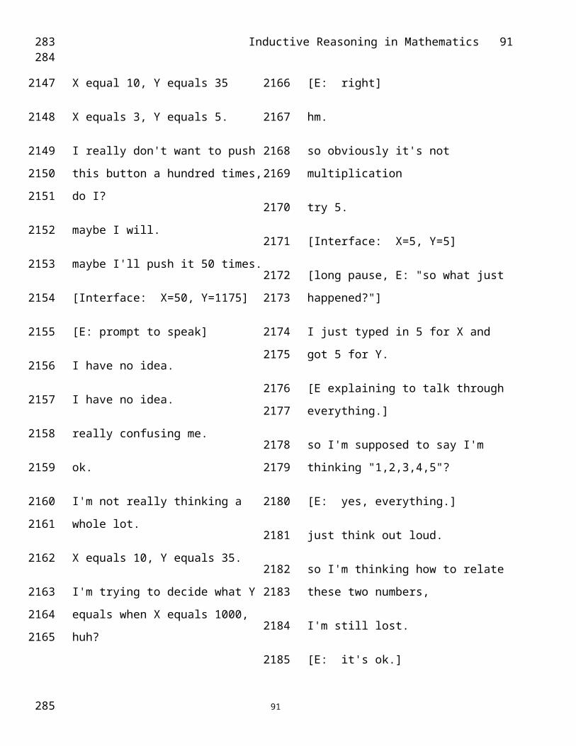
Inductive Reasoning in Mathematics 91
Table 11
PURSUIT Productions for Succeeding at F1
Production Action New Knowledge Quantities Compare to
1. Relate-by-multiplication S * __ = P A = (0 1/2 1 3/2 2) A = Y/X Ace's step 5.
2. Recognize-pattern:
differs-by-halves Pursue A Ace's step 7.
3. Examine-numerator B = (0 1 2 3 4) B = 2A
= 2*Y/X
4. Recognize-pattern:
counting-numbers Pursue B
5. Relate-by-subtraction S - __ = P X - B = (3 3 3 3 3)
6. Express-in-terms-of-X Hypo => P (X-3) = B Ace's step 8.
7. Unwind-multiplication Hypo/2 (X-3)/2 = A B/2 = A Ace's step 9.
8. Unwind-division (Hypo)*X X*((X-3)/2) = Y A*X=Y Ace's step 10.
9. Test-hypothesis X*((X-3)/2) = Y
10. Finish Problem F1:
Status = solved.
278
2052
2053
2054
2055
2056
2057
2058
2059
2060
2061
2062
279
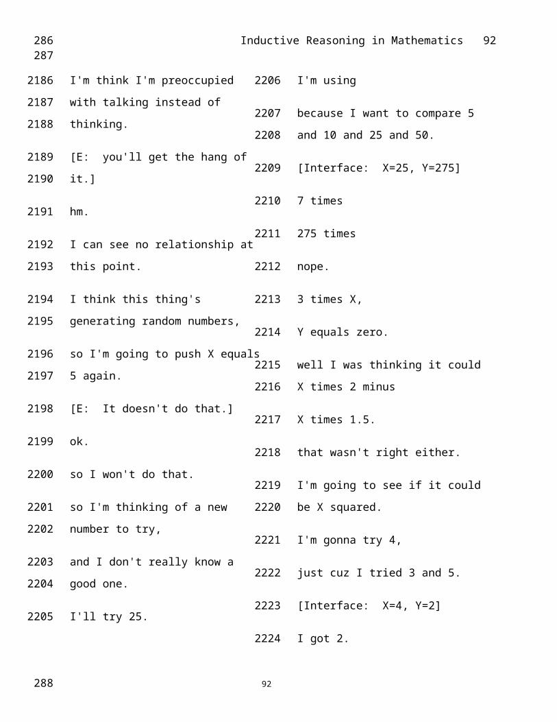
Inductive Reasoning in Mathematics 92
Table 12
PURSUIT Productions for Failing at F1
Production Action New Knowledge Quantities Compare to
1. Relate-by-multiplication S * __ = P A = (0 1/2 1 3/2
2)
A = Y/X Ace's step 5
Cannot fire "Recognize-pattern"
2. Relate-by-subtraction S - __ = P C = (-3 -2 0 3 7) C = Y-X
Cannot fire "Recognize-pattern"
3. Find-differences-within-
quantity
D = (_ 2 3 4 5) D = Ydiff Ace's step 2
4. Recognize-pattern:
counting-numbers Pursue D
5. Relate-by-subtraction S - __ = P X - D = (_ 2 2 2
2)
6. Express-in-terms-of-X Hypo = P (X-2) = D Ace's step 3
Cannot fire "Unwind" productions
IMPASSE Ace's step 5
280
2063
2064
2065
2066
2067
2068
2069
2070
2071
2072
281
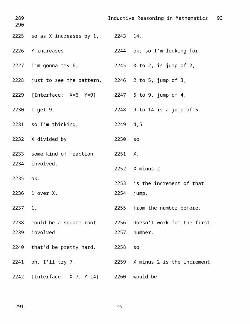
Inductive Reasoning in Mathematics 93
Table 13
PURSUIT Productions for Solving F2
Production Action New Knowledge Quantities
1. Relate-by-multiplication S * __ = P A = (3 5 7 9 11) A = Y/X
2. Recognize-pattern:
odd-numbers Pursue A
3. Relate-by-addition S + __ = P B = (2 3 4 5 6) B = A-X = Y/X -
X
4. Recognize-pattern:
counting-numbers Pursue B
5. Relate-by-addition S + __ = P B - X = (1 1 1 1 1)
6. Express-in-terms-of-X Hypo => P (X+1) = B
7. Unwind-subtraction Hypo+X X + (X+1) = A B+X = A
8. Unwind-division (Hypo)*X X*(2X+1) = Y
9. Test-hypothesis X*(2X+1) = Y
10. Finish Problem F2:
Status = solved.
282
2073
2074
2075
2076
2077
2078
2079
2080
2081
2082
2083
283

Inductive Reasoning in Mathematics 94
Figure Captions
Figure 1. Sample set of data for a function-finding problem
Figure 2. Given the measure of angle 1, find the measure of angle 2.
Figure 3. Example screen from data collection interface: collecting f(7) = 14.
Figure 4. Functions participants were asked to discover, with corresponding data
Figure 5. Overview of Ace's solution path
284
2084
2085
2086
2087
2088
2089
2090
285
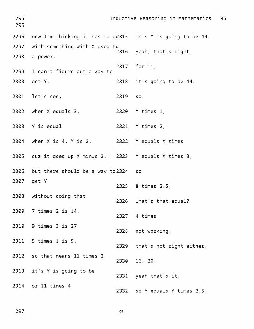
Inductive Reasoning in Mathematics 95
TOP
Figure 1
x 1 2 3 4 5 6
y 1 4 9 16 25 36
286
2091
2092
2093
2094
2095
2096
2097
2098
2099
2100
2101
2102
2103
287

Inductive Reasoning in Mathematics 96
TOP
Figure 2
∠1∠2
288
2104
2105
2106
2107
2108
2109
2110
2111
2112
2113
289

Inductive Reasoning in Mathematics 97
TOP
Figure 3
Data Interface
• • • • • • •
Click Here DONE
Answer:
Number of clicks: Number of answers left: 7 9
14
290
2114
2115
2116
2117
2118
2119
2120
2121
2122
2123
2124
291

Inductive Reasoning in Mathematics 98
TOP
Figure 4
X YFunction 1 (F1) 3 0y = x(x-3)/2 4 2
5 5f(1000) = 498,500 6 93 operations: -, *, ÷ 7 14
Function 2 (F2) X Yy = x(2x + 1) 1 3
2 10f(1000) = 2,001,000 3 213 operations: +, *, * 4 36
5 55
292
2125
2126
2127
2128
2129
2130
2131
2132
2133
2134
2135
2136
2137
2138
293

Inductive Reasoning in Mathematics 99
TOP
Figure 5
8 209 27
10 35
X Y3 04 25 56 97 14
Y Diff
2345
x - 2
x * (x-3)/2 = y
1 2
34
5
6
X * __ = Y
.51
2
2.53
8
9
7
in terms of X
(4-3) = 1(5-3)/2 = 1
(8-3)/2 = 2.5
(x-3)/2
10
Diff
1/21/21/21/2
q
294
2139
2140
2141
2142
2143
2144
2145
2146
2147
2148
2149
295

Inductive Reasoning in Mathematics 100
Footnotes
2One unsuccessful participant's protocol was lost due to mechanical failure. As a result, several
analyses are based only on the remaining 15 participants.
3Recall that 10 was the maximum number of instances that could be collected. Further
instances could be inferred, however, via pattern completion.
4Most (15 out of 16) participants collected either x=1 or x=2, as well, but here the interface,
rather than providing the value of y for these instances, produced the following message. "For
this problem, you cannot generate data for less than 3 clicks." The problem was designed in
this way to avoid the use of negative numbers in this experiment. Thus, the collection of these
instances is interesting only in that we know that participants were attempting to collect them,
and we know that the participants were thus provided with the information that their data
collection could not include x values less than 3. Some participants did form loose hypotheses
about the nature of the sought-after rule based on this information (such as the correct
hypothesis that the y-values of the function would be negative below the point where x=3.)
Note that the request for x=1 or x=2 did not count toward the 10 instances allowed to the
participant.
5One solved the problem very quickly, and thus had an extremely short protocol. This
participant's protocol had only one series of codable episodes before reaching the answer, and
this entire episode was coded as HG and thus accounts for the apparent disproportionate
allocation of effort for this participant. The other participant found the solution to the problem
through the use of a recursive formula and Gauss' formula for the summation of n sequential
296
2150
2151
297
298
299
300
301
302
303
304
305
306
307
308
309
310
311
312
313
314
315
316
317

Inductive Reasoning in Mathematics 101
integers. This approach resulted in an unusual amount of PF for this participant.
6An example route: plug in "x-2" for "n" to produce [x-2]*([x-2]+1)÷2. As the formula is for a
sequence starting at 1 instead of at 2, we subtract 1 from it: ([x-2]*([x-2]+1)÷2) - 1. Now
reduce: ((x-2)*(x-1)÷2) - 1 = ((1/2)x2 - (3/2)x + 1) - 1 = (1/2)x2 - (3/2)x = (1/2)(x2- 3x) =
(1/2)x(x-3). Voila.
7"Detecting the pattern" means noting in one way or another, and either on paper or verbally,
that q increases by a constant for each sequential value of x.
8Discovering that the quantity (y-x)/x can be expressed in terms of x as (x-5)/2 will lead to the
final solution as follows: (y-x)/x = (x-5)/2. (y-x) = x*(x-5)/2. y = x + x*(x-5)/2 = x + x*(x/2 -
5/2) = x + (1/2)x2 - (5/2)x = (1/2)x2 - (3/2)x = (1/2)x*(x-3).
9A pilot study suggests some support for this notion. In the study, participants were asked to
assess how difficult it would be to have to find the function for each of several sets of x and y
data. Participants rated the data for y/x from F1 (.5, 1, 1.5, 2,... ) as more difficult to
potentially induce than the data for y itself (2, 5, 9, 14,... ), although in actuality this is not the
case. In contrast, for F2, they rated y/x (3, 5, 7, 9,... ) as simpler than y itself (3, 10, 21, 36,... ).
10For example, one could take the differences between the successive y-values. If these are
constant, then that constant is the coefficient of x, and the function is linear. If these y
differences are not constant, but differ by a constant, then that constant is twice the coefficient
of the x2 term and the function is quadratic. Similar algorithms can be used for higher-powered
polynomials.
318
319
320
321
322
323
324
325
326
327
328
329
330
331
332
333
334
335
336
337
338
339