Electronic copy available at: http://ssrn.com/abstract=2147012

Running head: STAT ARB & HFT

Statistical Arbitrage Trading Strategies and High Frequency Trading

Thomas A. Hanson

Kent State University

Joshua R. Hall

Kent State University

January 13, 2013

Correspondence concerning this article should be addressed to Thomas A. Hanson,

Kent State University, College of Business Administration, Department of Finance,

P.O. Box 5190, Kent, Ohio, 44242. Phone: (330) 672 – 1129. Fax: (330) 672 – 9806.

E-mail: thanson3@kent.edu

Electronic copy available at: http://ssrn.com/abstract=2147012

STAT ARB & HFT 2

Statistical Arbitrage Trading Strategies and High Frequency Trading

Abstract

Statistical arbitrage is a popular trading strategy employed by hedge funds and proprietary

trading desks, built on the statistical notion of cointegration to identify profitable trading

opportunities. Given the revolutionary shift in markets represented by high frequency trading

(HFT), it is unsurprising that risks and rewards have changed. This paper explores the effect of

HFT volume on statistical arbitrage profitability, and reports three trends in the data. First,

higher levels of comovement due to HFT cause more stock pairs to be cointegrated over time.

Second, profitability from statistical arbitrage remains steady among the vigintiles with the most

HFT. Third, the range of profitability is larger in more recent years. These findings suggest that

HFT increases correlation and volatility and has a direct impact on statistical arbitrage trading

strategies.

Keywords: Statistical arbitrage, pairs trading, cointegration, high frequency trading

Electronic copy available at: http://ssrn.com/abstract=2147012

STAT ARB & HFT 3

Statistical Arbitrage Trading Strategies and High Frequency Trading

1.0 Introduction

The trading of common stocks in the U.S. markets is now dominated by computer

algorithms operating at sub-second speeds (Schapiro, 2010). This state of affairs represents the

natural extension of quantitative strategies through the use of ever improving technology. One

of the many available trading strategies that is ideally suited for such an application is statistical

arbitrage, which involves forming a pair or portfolio of stocks whose relative pricing differs from

their long-run equilibrium.

The roots of statistical arbitrage can be traced to the long-short mutual fund investment

strategies of A. Winslow Jones in the 1950s. His idea was to use fundamental analysis to create

a hedged portfolio of long and short positions to eliminate market risk. The return on the

portfolio comes from the relative performance of the positions. So long as the long position

gains more, or loses less, than the short position, the portfolio will be profitable. This can be true

even in a mostly flat market, and the search for profits in difficult markets has made various

incarnations of long-short investing popular since that time (Jacobs & Levy, 1993). Statistical

arbitrage1 is a quantitative application of this concept, based principally on price history (in

addition to any screening traits for the candidate stocks for the portfolios).

The strategy gained prominence in the mid-1980s when Nunzio Tartaglia assembled a

group of traders to create computer models that could efficiently access and analyze more data at

faster speeds than previously possible. This timing reveals that pairs trading was among the

earliest trading algorithms, replacing fundamental valuation, intuition, and trading skills with

1The term statistical arbitrage, as it is generally used, encompasses a range of investment strategies that share formal

characteristics outlined in section two. When the long and short portfolios are restricted to a long position in just

one stock and a short position in another, the implementation is often referred to as pairs trading, and both

descriptive terms will be used interchangeably in this paper except where a distinction becomes necessary.

STAT ARB & HFT 4

quantitative rules for a computer to check and implement. Early profitability also coincides with

the faster trading and higher volumes in U.S. equity markets. Hence, it might be suggested that

faster processing and more volume in equity markets would enhance profits for statistical

arbitrage strategies.

High frequency trading (HFT, also used for high frequency traders) is widely

acknowledged as a revolutionary and dominant force in equity markets and has grown at an

astonishing pace to represent the majority of trading on the world’s major exchanges (Curran &

Rogow, 2009; Schapiro, 2010). Its new prominence has implications for market quality

(Brogaard, 2010), the cost of transacting (Menkveld, 2012), liquidity (Hendershott, Jones, &

Menkveld, 2011), price efficiency (Brogaard, Hendershott, & Riordan, 2011), correlation

structure (Hanson & Muthuswamy, 2011), and a range of other effects in recent finance

literature. It is unsurprising that such major market changes would impact the profitability of

quantitative trading strategies.

Additionally, it is generally assumed that as knowledge of arbitrage opportunities

becomes more widely dispersed, it becomes more difficult to profit from such strategies.

However, some pricing anomalies continue to persist. Of particular relevance to pairs trading is

the issue of contrarian profits (Jegadeesh & Titman, 1995). Profits from pairs trading might stem

in part from investor over-reaction. One question this raises is whether HFT inhibits or promotes

volatility and over-reaction that would enhance such profits. This question remains unresolved

and widely disputed.

From the point of view of market efficiency, it would be logical that statistical arbitrage

opportunities would decrease over time, especially as HFT took advantage of ever-smaller

mispricings at ever-faster speeds. In theory, one could make a case for HFT as a force for

STAT ARB & HFT 5

decreased profitability or increased trading opportunities. Therefore, the principal contribution

of this paper is an exploration of whether HFT increases or decreases the profits of statistical

arbitrage trading strategies over time and across different levels of HFT volume.

The remainder of the paper proceeds as follows. The next section briefly reviews the

literature related to both statistical arbitrage and HFT. Section three describes the data, the

challenge of measuring HFT, and the pairs trading scheme. The fourth section presents results,

and the fifth section concludes.

2.0 Literature Review

The trading strategy under consideration in this paper concerns the intersection of two

topics: statistical arbitrage and high frequency trading. The pairs trading phenomenon has been

well known for some time and spawned a range of papers on its profitability, in addition to

implementation in industry. This section briefly reviews some of the major papers on the topic

of pairs trading. Following that, we discuss the possible changes in the profitability of pairs

trading in a high frequency trading environment. We are aware of only one other paper (Bowen,

Hutchinson, & O’Sullivan, 2010) that has explored this overlap. That research closely examines

the sensitivity of pairs trading profits to transaction costs and speed of execution.

Our work differs in several ways. First, the research question is whether stocks with

different HFT volume behave differently in terms of the profitability of a statistical arbitrage

trading scheme. The examination is a comparison of profitability across HFT volume vigintiles,

rather than costs and speed across the entire universe of stocks. Second, the sample period under

consideration here is considerably larger. Finally, Bowen, Hutchinson, and O’Sullivan (2010)

employ a sum of squared deviations ranking, rather than cointegration testing, as employed in

our study. The details of our trading scheme are delayed until section three.

STAT ARB & HFT 6

2.1 Statistical Arbitrage Strategies

Statistical arbitrage is a strategy that attempts to profit from relative mispricing based on

historical price patterns. Unlike true arbitrage, it is not riskless. Bondarenko (2003) defines a

statistical arbitrage opportunity as a zero-cost trading opportunity for which the average expected

payoff is nonnegative. In other words, the strategy must have an expectation of profit at

inception, but losses are possible ex post. The definition is extended by comparison to standard

option pricing models by Hogan, Jarrow, Teo, and Warachka (2004). In their work, a statistical

arbitrage opportunity remains self-financing and zero-cost as well as satisfying four conditions:

the discounted profit at inception is zero, and in the limit over a time span approaching infinity

the expected profit is positive, the probability of loss is zero, and finally the time-averaged

variance converges to zero when there is a positive probability of loss at all times.

True implementation of these formal definitions of statistical arbitrage requires

continuous time rebalancing, in the spirit of the Black-Scholes option pricing model. In

empirical work and industry practice, it is more typical for the long-short ratio to be fixed for a

given trading period (e.g., Whistler, 2004). This introduces additional risk but limits transaction

and monitoring costs considerably. Furthermore, it simplifies the actual trading strategy and

moves the focus of research toward the task of identifying pairs that are likely to be profitable.

Previous research has utilized three main methods for identifying candidate pairs. First,

the distance method ranks pairs by the sum of squared differences between the normalized price

series (Gatev, Goetzmann, & Rouwenhorst, 2006). Second, the stochastic spread approach was

proposed by Elliot, van der Hoek, and Malcolm (2004). This work models the spread explicitly

in a continuous time setting, which is useful for modeling mean reversion and forecasting the

STAT ARB & HFT 7

spread. However, it has a serious drawback because it formally requires both stocks in the

candidate pair to have the same long run return, which is unlikely in practice.

The third and final identification strategy, and the one employed in the present study,

employs the statistical phenomenon of cointegration (Engle & Granger, 1987) to identify

candidate pairs. A formal discussion of this approach is postponed until the next section, but

intuitively it is a long-term relationship between nonstationary time series. Cointegration is

sometimes colloquially described as a drunk man leading a dog on a leash; while each might

wander in a seemingly random pattern, they are connected and cannot drift arbitrarily far apart.

If two stock prices are linked in such a way, their prices are likely to revert toward their long-run

relationship, yielding profit for a statistical arbitrage strategy. The application of cointegration to

pairs trading is discussed extensively in Vidyamurthy (2004).

The theoretical basis for the cointegration approach is rooted in arbitrage pricing theory

(APT, Ross, 1976). In particular, Vidyamurthy (2004) argues that the cointegrating relationship

is due to a proportional shared risk exposure (whose source is likely unknown and even left

unexplored in a purely quantitative implementation). However, Do, Faff, and Hamza (2006)

note that this interpretation is somewhat problematic because APT posits the total return to be

due to the sum of the risk free rate and the return to risk factor exposure. Thus, pairs trading

through cointegration is only heuristically linked to mainstream asset pricing models.

The strategy is often also likened to an application of the Law of one Price. If two stocks

are expected to have similar returns (or cash flows) in the future, then their prices should be near

each other. Or, in relative terms, if their returns generally follow the same trend, then their price

histories should trace similar paths over time.

STAT ARB & HFT 8

Among the most widely cited applied work in this area is Gatev, Goetzmann, and

Rouwenhorst (2006), who examine daily price data from 1962 to 2002 and yield average

annualized excess returns of nearly 11%. They also demonstrate that returns to pairs trading

have declined over time, with profits lower in the period after 1989. This finding is reinforced

by Chen, Chen, and Li (2012), who suggest that the participation of more arbitrageurs has eroded

profitability. To the extent that HFT employ statistical arbitrage strategies, they will eliminate

the mispricing and through their competition remove any profits to be made in simple pairs

trading algorithms.

The reasonable argument that HFT would destroy pairs trading profitability has not been

fully borne out in practice. Like some other pricing anomalies, profitability persists. In one

recent study Bowen, Hutchinson, and O’Sullivan (2010) demonstrated that pairs trading

remained a profitable strategy during 2007 for the FTSE100 constituent stocks. Perlin (2007)

showed profitability in the Brazilian market continued at least through 2006, and Siy-Yap (2009)

demonstrated a declining but still profitable implementation in the Canadian market. These

examples demonstrate persistence of profitability across a range of trading environments by

encompassing the very liquid, high volume environment of the London Stock Exchange and the

still developing stock market of Brazil. In any case, the ongoing anomaly suggests the need for

further scrutiny of the strategy’s profitability in a market characterized by HFT.

2.2 The High Frequency Trading Environment

The effects of HFT on various aspects of markets (including liquidity, trading costs, price

efficiency, and correlation) have been widely debated and studied in recent years, sometimes

with uncertain or conflicting conclusions. Of particular interest here is the effect of HFT on

correlations among equities. Casual empiricism reveals that in recent years correlations among

STAT ARB & HFT 9

U.S. equities have increased significantly; this has decreased the effectiveness of stock picking

strategies for diversification (e.g., Lauricella & Zuckerman, 2010; Jannarone, 2011). This trend

is often attributed to the presence of HFT in the market. The tendency toward generally higher

correlations has been formally established in a growing body of literature (Erb, Harvey, &

Viskanta, 1994; Longin & Solnik, 1995), and the concept of correlation risk is now prevalent

enough that it can be considered a priced risk in portfolio construction (Krishnan, Petkova, &

Ritchken, 2009; Buraschi, Porchia, & Trojani, 2010). Of most direct applicability, the link

between rising correlations and high frequency trading was explored by Hanson and

Muthuswamy (2011).

Higher correlations have two possibly offsetting effects on pairs trading profitability.

First, comovement among stocks will likely raise the number of cointegrated pairs to be

candidates for pairs trading. Second, higher levels of comovement make it less likely that pairs

will diverge to a large enough extent that trading the spread will be profitable. In other words,

there will likely be more trading opportunities at smaller profit margins, and one might expect

such profits to be taken quickly by high frequency traders.

Faster convergence to efficient market prices would further bolster the position for lower

profits from pairs trading. Arguing along those lines, Brogaard, Hendershott, and Riordan

(2011) suggest that HFT increases price efficiency by trading in the same direction as permanent

price changes but opposite to short term market fluctuations. In a comparison of the Shanghai,

Shenzhen, and Hong Kong stock exchanges, Mai and Wang (2011) conclude that more efficient

markets lead to lower profits for pairs trading strategies. Similarly, Andrade, di Pietro, and

Seasholes (2005) report that pairs trading profits are correlated with uninformed trading. Since

HFT is usually implemented by sophisticated investors with an information and speed advantage,

STAT ARB & HFT 10

higher participation by HFT would be expected to limit pairs trading profitability. These

previous studies suggest that within the U.S. market stocks with higher concentration of HFT

would be less attractive for statistical arbitrageurs.

By contrast, in a significant theoretical paper, Froot, Scharfstein, and Stein (1992)

develop a model in which short-horizon traders cause markets to become less efficient.

Furthermore, HFT can be motivated not by firm fundamentals but rather trade flow, a

phenomenon sometimes termed flow toxicity (Arnuk & Saluzzi, 2008; Easley, Prado, & O’Hara,

2012). To the extent that toxic order flow is present in markets, prices can reflect the popularity

of a given strategy, macroeconomic news, or even investment sentiment and rumor. This might

cause increased volatility and more mispricing opportunities due to temporary overreactions

from HFT. Such an outcome would imply more profitable opportunities among stocks with

greater levels of HFT volume.

Given the division in the literature and past results, the data and testing in the remainder

of this paper is exploratory in nature, seeking to answer two questions. One, does the previously

observed trend toward lower profitability from a pairs trading strategy continue with more recent

market data? Two, is there a difference in this effect due to high frequency trading volume?

3.0 Data and Method

The sample for this study is comprised of all common stocks (CRSP share codes 10 and

11) that trade above $1 and are included in both the CRSP and Thomson Reuters Institutional

Holdings databases from 1985 to 2011. In additional screening, stocks that have one or more

days with zero volume are eliminated from the sample. This ensures a minimal level of liquidity

in the candidate stocks. The total sample includes 371,416 firm-quarter observations, which is

STAT ARB & HFT 11

split, as explained below, into a training period from 1985 to 1994 (118,060 firm-quarters) and a

trading period from 1995 to 2010 (253,356 firm-quarters).

One necessary data correction involves the Thomson Reuters data on net changes in

shares held by institutions. As Zhang (2010) notes, from the second quarter of 2006 through the

first quarter of 2007 the net changes are incorrectly reported as the previous quarter’s stock

holdings multiplied by negative one. Therefore, we manually recalculate the net change data for

these quarters by taking the difference in share reported holdings in adjacent quarters.

3.1 Estimating HFT volume

Market data do not allow for direct observation of HFT volume. This complication has

spawned a number of proxies and differing methodologies within the industry and among

researchers. Proprietary research, such as that conducted by the TABB Group, generally attempt

to identify trading activity by firms that operate primarily with HFT strategies (e.g., Getco and

Citadel). A form of this direct identification is now available for academic research through the

NASDAQ, which supplies data under a non-disclosure agreement. These data have been

utilized, for example, by Brogaard, Hendershott, and Riordan (2011) in their examination of

HFT’s effect on price discovery.

The NASDAQ data remain problematic, however, for several reasons. First, the

information is drawn from a stratified sample of just 120 stocks. Second, the identification of

HFT is done by NASDAQ, which impairs replicability and transparency. Third, it fails to

provide an out-of-sample model that can be used to estimate HFT across a broader time span.

Therefore, while the NASDAQ data provide an intriguing opportunity for study, they are

applicable in all situations. In particular, the present study requires a technique to calculate

STAT ARB & HFT 12

approximate HFT activity over a nearly twenty year span of time and for a broad range of

equities.

Zhang (2010) proposes one such method for estimating HFT volume through the use of

data available from CRSP and the Thomson Reuters Institutional Holdings databases. The

measure is built on a turnover-based identity, in which total trading volume is subdivided into

three classifications, based on the participants involved: individual investors, institutional

investors, and high frequency traders. Further refinements lead to observable variables in the

following equation:

TO = INSTTO*INST + INDIVTO*INDIV + HFT

in which TO is total stock turnover, INSTTO is institutional turnover, INDIVTO is individual

turnover, INST and INDIV are (respectively) institutional holdings and individual holdings as a

fraction of total shares outstanding. Three of these variables, namely TO, INST, and INSTTO,

are observable from the CRSP and Thomson Reuters databases. Figure 1 displays these series

over the entire sample period. Most noticeable is the strong uptick in market turnover (TO) that

begins in the mid-1990s but abates somewhat following the credit crisis of 2008.

Three further assumptions are necessary to facilitate an estimate of HFT. First, it is

assumed that no high frequency trading existed prior to the beginning of 1995. This choice of

date by Zhang (2010) is apparently ad hoc, due to visual examination of turnover data.

Pinpointing the beginning of HFT is impossible because it represents a gradual, evolutionary

change in the market. Its origins can be traced at least as far back as the SOES “bandits” of the

late 1980s (Patterson, 2012), and HFT was certainly in force by the time of price decimalization

in 2000. Using piecewise linear regression to search for a single breakpoint that minimizes the

STAT ARB & HFT 13

sum of squared errors for the turnover data suggests the beginning of 1993 as the date when HFT

began to increase market turnover.

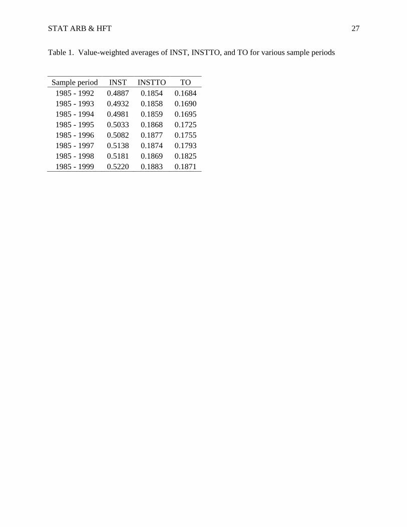
The truly relevant question is how much the choice of sample period influences average

measures of the market during the estimation period. Table 1 displays value-weighted averages2

of institutional holdings, institutional turnover, and total market turnover for various sample

periods. The sample always begins in 1985 and the ending year varies from 1992 through 1999.

Throughout this period, the averages are quite stable, suggesting that the HFT measurement is

robust to the precise specification of the estimation period. Therefore, while acknowledging the

multiplicity of possible dates, we choose to follow Zhang (2010) and use the start of 1995 as the

date when HFT began in earnest.

The second assumption is that HFT do not hold positions at the end of any quarter. This

strong assumption is justified by the short holding periods of HFT strategies and the general goal

of carrying no overnight inventory. It implies that INDIV + INST = 1 at all times when

examining market closing data.

Third, Zhang (2010) assumes that the trading behavior of individuals relative to

institutions remains stable over time. He is quick to point out that this does not require stable

patterns of behavior, but rather a stable ratio. Individuals and institutions will tend to trade more

or fewer shares in tandem with one another so that the ratio of their turnover is stable.

In calculating total market turnover, an adjustment is necessary for the potential double-

counting of dealer trades of NASDAQ stocks (Gould & Kleidon, 1994). The over-reporting of

volume on the NASDAQ was examined by Atkins and Dyl (1997), who documented an

approximate 50 percent drop in volume for the stock of firms switching from NASDAQ to

2 Value-weighted averages are calculated throughout this paper by using average market capitalization for each firm-

quarter observation. We believe that one source of slight discrepancies between our calculations and Zhang’s could

be due to different weighting schemes.

STAT ARB & HFT 14

NYSE. For this reason, Zhang (2010) suggests using half of the reported volume for NASDAQ

stocks.

There is some evidence, however, that the problem of inflated volume for NASDAQ

stocks has diminished in recent years. Anderson and Dyl (2005) find that the decrease in volume

has declined to 38% over the five-year period ending in 2002. They suggest a number of

structural changes in the market that could combine to cause this change, including the growth of

ECNs, competition from public limit orders, and rule changes put in place for reporting of trades

to the NASDAQ. Furthermore, they note that firms with high daily volume on average

experience a greater rate of over-counting and suggest that a separate adjustment factor be used

for high- and low-volume stocks. By following Zhang (2010) and dividing NASDAQ volume

by two, it is plausible that the present investigation understates total market turnover in the more

recent years of the sample period. Due to this, the calculated HFT volume is also likely

understated.

The procedures outlined above allow for an estimation of the ratio of individual turnover

to institutional turnover (INSDIVTO/INSTTO). Zhang (2010) estimates this ratio to be 71.81%,

while our sample yields an estimate of 82%. The differential could arise due to different samples

and different weighting criteria, and the results here suggest lower levels of HFT volume in the

market: 71% of volume in the U.S. market in 2009, compared to Zhang’s (2010) estimate of 78%

and the TABB Group’s estimate of 73%.

The actual level of HFT volume for the various stocks is not used directly in any further

calculations in this study. Instead, the stocks are ranked by this measure and split into vigintiles

for use examination of pairs trading profitability. Since the rankings will be robust to the

particular estimate, we retain our figure of 82% and calculate HFT using the following equation:

STAT ARB & HFT 15

HFT = TO – INSTTO*INST – (0.82*INSTTO)*(1 – INST)

This variable is calculated for each firm-quarter observation in the sample, and stocks are ranked

within each quarter and split into vigintiles portfolios for further testing.

3.2 Cointegration testing

Cointegration can be conceptually described as a long-run equilibrium relationship

between two (or more) nonstationary time series. Independently, two nonstationary time series

will wander unpredictably, but there exists a linear combination of those same variables that is

stationary. Figure 2 provides an example of two stocks that are cointegrated. Their price history

follows common trends, and the two price series appear to revert toward parity whenever they

drift apart. This is reinforced in Figure 3, which plots the spread between the two stocks. The

spread is a stationary process, with multiple crossings of its (near zero) mean value. This

reversion property of the spread is what creates a profitable trading opportunity, as outlined in

this and the next section.

Granger (1981) formally introduced cointegration and coined the term, while the first

formal test for cointegration was presented by Engle and Granger (1987). In the context of

financial time series, their two-step approach begins by regressing the log price of stock A on the

log price of stock B, which implies the following relationship:

( ) (

) ,

with γ called the cointegrating coefficient and the constant term μ the premium of stock A versus

B. This regression has been termed superconsistent because the estimate ̂ converges to its true

value at a rate of T, rather than the usual convergence rate of ⁄ (Stock, 1987).

Due to market efficiency, it is assumed that the log price series are random walks and

hence nonstationary. If the two series are cointegrated, however, the appropriately constructed

STAT ARB & HFT 16

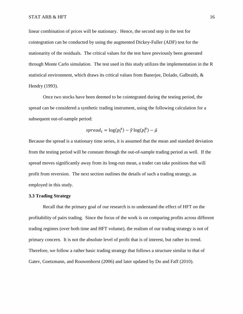
linear combination of prices will be stationary. Hence, the second step in the test for

cointegration can be conducted by using the augmented Dickey-Fuller (ADF) test for the

stationarity of the residuals. The critical values for the test have previously been generated

through Monte Carlo simulation. The test used in this study utilizes the implementation in the R

statistical environment, which draws its critical values from Banerjee, Dolado, Galbraith, &

Hendry (1993).

Once two stocks have been deemed to be cointegrated during the testing period, the

spread can be considered a synthetic trading instrument, using the following calculation for a

subsequent out-of-sample period:

( ) ̂ (

) ̂

Because the spread is a stationary time series, it is assumed that the mean and standard deviation

from the testing period will be constant through the out-of-sample trading period as well. If the

spread moves significantly away from its long-run mean, a trader can take positions that will

profit from reversion. The next section outlines the details of such a trading strategy, as

employed in this study.

3.3 Trading Strategy

Recall that the primary goal of our research is to understand the effect of HFT on the

profitability of pairs trading. Since the focus of the work is on comparing profits across different

trading regimes (over both time and HFT volume), the realism of our trading strategy is not of

primary concern. It is not the absolute level of profit that is of interest, but rather its trend.

Therefore, we follow a rather basic trading strategy that follows a structure similar to that of

Gatev, Goetzmann, and Rouwenhorst (2006) and later updated by Do and Faff (2010).

STAT ARB & HFT 17

Statistical arbitrage strategies based on cointegration all follow the same basic three part

format. First, an initial universe of candidate stocks is identified. This preliminary step allows a

trading scheme focused on a particular industry or other subset that might be presumed to have a

high degree of comovement in stock returns. Second, the candidate pairs are tested for

cointegration using the chosen statistical test, and the spread is calculated from those results.

Third, when the spread widens beyond some predefined threshold, the trader takes the

appropriate long and short positions to profit from reversion to the long run relationship.

The implementation employed here follows a two-stage structure. The first stage

(training period) consists of one year of daily price observations for a broad universe of

candidate stocks: all stocks priced over one dollar and with at least one reported trade each day.

These stocks are sorted into vigintiles based on HFT volume, as calculated from Zhang’s (2010)

methodology. Each vigintile contains between 353 (in 2010) and 501 (in 1997) different stocks.

The one-year training periods coincide with the calendar year and are non-overlapping, yielding

16 distinct trading periods for comparison. (Note that the subsequent trading period does overlap

with another training period.)

Within each vigintile, all possible pairs are tested for cointegration using the Engle-

Granger two-step procedure. By testing all possible pairs, this process does not consider other

variables that are sometimes included in cointegration analysis, namely a desire for market

neutrality (for example, β spread less than 0.2) or a consideration of matching stocks based on

industry, size, book-to-market, or any other characteristic (some of these are utilized by

Velayutham, Lukman, Chiu, & Modarresi [2010]). By running the cointegration test across all

stocks within the HFT vigintile, this study identifies the largest universe of cointegrated stocks.

At the same time, it can increase the risk of trading any particular pair. The desire to emphasize

STAT ARB & HFT 18

the influence of HFT motivated the omission of further screening variables. Therefore, any pairs

whose residuals are determined stationary by the ADF test at a 10% level of significance are

considered trading candidates in the stage two of the trading algorithm.

In the second stage, the regression coefficients from the Engle-Granger test are used to

construct the spread for all cointegrated pairs on an out-of-sample trading period of 125 days.

The spread is then treated as a synthetic investment vehicle, with a trader taking the appropriate

long and short positions to profit from a rise or fall in the spread. The mechanical trading rule

employed here is to enter a trade whenever the spread moves more than two standard deviations

away from its mean (with the mean and standard deviation calculated from the training period

and considered constant over the entire trading period). The trade is exited at a profit if the

spread reverts and crosses its mean value. The trade is exited at a loss if the spread widens to

more than three standard deviations from the mean. Finally, all pairs are closed at the end of the

125-day trading period, regardless of the profit or loss incurred.

Figure 4 depicts one example of the trading process for a cointegrated pair. The time

period displayed is of the trading period only (125 days). The top panel shows the spread, which

in this case spends most of the trading period below its mean value from the training period. The

dotted lines represent levels two and three standard deviations below the mean (respectively, the

entry and stop loss signals). The middle panel is a depiction of the trading signal, which takes a

zero value when there is no position and a one otherwise. Finally, the bottom graph portrays the

cumulative profit from the investment rule. In this particular example, there are three times that

the trade is entered. The first ends in a loss when the spread moves below the third standard

deviation, while the second and third periods end in a profit when the spread moves below the

two-standard deviation line and reverts to the mean. Overall, this is a profitable pairs trade.

STAT ARB & HFT 19

Log returns from the trading strategy are calculated as the cumulative sum of the

difference of the spread. This carries the implicit assumption that cash flows neither earn nor

incur any interest costs. Furthermore, there is no consideration of capital not invested in the

strategy. Instead, the portfolio return is based on equal investments in all available pairs

whenever the trading criteria are met. Again, this is a very basic trading strategy, and the level

of profits is not of direct interest. Rather, the results in the next section are focused on the

differences in profitability over time and across vigintiles of HFT volume.

4.0 Results

Table 2 (Panels A and B) presents results on the percentage of pairs within each vigintile

that are identified as cointegrated using the Engle-Granger two-step procedure and a 10%

significance level in the ADF test of the residuals. Two trends are readily evident from the

results. First, a higher percentage of candidate pairs are identified as cointegrated in more recent

years. For example, in the vigintile with the greatest HFT volume, cointegrated pairs increase

from 18.4% in 1995 to 32.7% in 2010. Though the effect is certainly not monotonic, it is the

general trend across all vigintiles. This suggests that the trend toward higher comovement in the

market dominates. This creates more trading signals for further scrutiny in the trading scheme.

The second general trend is that stocks with higher levels of HFT also have a greater

percentage of cointegrated pairs within a given year. For instance, in 2010, the vigintile with the

lowest HFT volume had only 9.0% of its pairs cointegrated, while the highest vigintile had

32.7% of pairs identified as cointegrated. Stocks with higher levels of HFT are more likely to

have similar return series and be cointegrated.

The stocks identified as cointegrated are then examined for their trading signals and

profits or losses, using the trading strategy outlined above. Results appear in Table 3. At least

STAT ARB & HFT 20

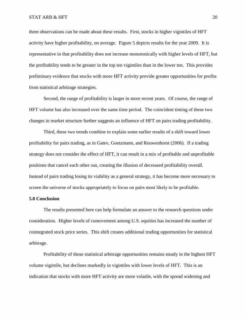
three observations can be made about these results. First, stocks in higher vigintiles of HFT

activity have higher profitability, on average. Figure 5 depicts results for the year 2009. It is

representative in that profitability does not increase monotonically with higher levels of HFT, but

the profitability tends to be greater in the top ten vigintiles than in the lower ten. This provides

preliminary evidence that stocks with more HFT activity provide greater opportunities for profits

from statistical arbitrage strategies.

Second, the range of profitability is larger in more recent years. Of course, the range of

HFT volume has also increased over the same time period. The coincident timing of these two

changes in market structure further suggests an influence of HFT on pairs trading profitability.

Third, these two trends combine to explain some earlier results of a shift toward lower

profitability for pairs trading, as in Gatev, Goetzmann, and Rouwenhorst (2006). If a trading

strategy does not consider the effect of HFT, it can result in a mix of profitable and unprofitable

positions that cancel each other out, creating the illusion of decreased profitability overall.

Instead of pairs trading losing its viability as a general strategy, it has become more necessary to

screen the universe of stocks appropriately to focus on pairs most likely to be profitable.

5.0 Conclusion

The results presented here can help formulate an answer to the research questions under

consideration. Higher levels of comovement among U.S. equities has increased the number of

cointegrated stock price series. This shift creates additional trading opportunities for statistical

arbitrage.

Profitability of those statistical arbitrage opportunities remains steady in the highest HFT

volume vigintile, but declines markedly in vigintiles with lower levels of HFT. This is an

indication that stocks with more HFT activity are more volatile, with the spread widening and

STAT ARB & HFT 21

reverting often enough to provide profit for appropriate positions to trade the synthetic trading

instrument based on the spread. This study thus contributes to the literature on HFT, in addition

to an understanding of pairs trading in modern markets.

In extensions of the current work, we intend to analyze returns in excess of other risk

factors, including the Fama-French three factor model. Portfolios will also be split by market

capitalization to ensure that HFT is distinct from size as an influence on pairs trading

profitability. The preliminary results presented here demonstrate that further research and

refinement is likely to be fruitful.

One limitation of this study is the use of daily closing prices. To the extent that HFT

employs statistical arbitrage strategies, they likely enter and exit positions at a much faster pace

than would be captured in the data. We are currently working on an extension of the testing

presented here on a high frequency data sample. However, we contend that daily data remain

important in revealing the overall market trend. Furthermore, daily prices allow comparison

over a long time horizon, more so than will be possible with higher frequency data.

Additionally, the HFT proxy employed is based on firm-quarter observations, so further

refinement below daily pricing begins to raise questions about the time-scale discrepancies

among the variables. Finally, the use of daily data allows direct comparison to previous

literature.

Results here apply to the U.S. stock market and could likely be replicated in other

developed markets around the world. An interesting extension of the work would be to examine

markets with different volumes of HFT, levels of development, and microstructural

characteristics. Also, statistical arbitrage is not limited to pairs trading, nor is it limited to the

equity market. The strategy can be implemented in index tracking, basket portfolios, and

STAT ARB & HFT 22

derivatives markets. We leave it for future research to consider the effect, if any, of HFT in

those settings.

STAT ARB & HFT 23

References

Anderson, A., & Dyl, E. (2005). Market structure and trading volume. Journal of Financial

Research, 28, 115 – 131.

Andrade, S., di Pietro, V., & Seasholes, M. (2005). Understanding the profitability of pairs

trading. Working paper.

Arnuk, L., & Saluzzi, J. (2008). Toxic equity trading order flow and Wall Street. White paper.

Atkins, A., & Dyl, E. (1997). Market structure and reported trading volume: NASDAQ vs. the

NYSE, Journal of Financial Research, 20, 291 – 304.

Banerjee, A., Dolado, J., Galbraith, J., & Hendry, D. (1993). Cointegration, Error Correction,

and the Econometric Analysis of Non-Stationary Data. Oxford: Oxford University Press.

Bondarenko, O. (2003). Statistical arbitrage and security prices. Review of Financial Studies,

16, 875 – 919.

Bowen, D., Hutchinson, M., & O’Sullivan, N. (2010). High frequency equity pairs trading:

Transaction costs, speed of execution, and patterns in returns. Working paper.

Brogaard, J. (2010). High frequency trading and its impact on market quality. Working paper.

Brogaard, J., Hendershott, T., & Riordan, R. (2011). High frequency trading and price

discovery. Working paper.

Buraschi, A., Porchia, P., & Trojani, F. (2010). Correlation risk and optimal portfolio choice.

Journal of Finance, 65, 393 – 420.

Chen, H., Chen, S., & Li, F. (2012). Empirical investigation of an equity pairs trading strategy.

Working paper.

Curran, R., & Rogow, G. (2009, June 19). Rise of the (market) machines. Wall Street Journal.

STAT ARB & HFT 24

Do, B., & Faff, R. (2010). Does simple pairs trading still work? Financial Analysts Journal,

66, 83 – 95.

Do, B., Faff, R., & Hamza, K. (2006). A new approach to modeling and estimation for pairs

trading. Working paper.

Easley, D., Prado, M., & O’Hara, M. (2012). The volume clock: Insights into the high

frequency paradigm. Working paper.

Elliott, R., van der Hoek, J., & Malcolm, W. (2005). Pairs trading. Quantitative Finance, 5,

271 – 276.

Engle, R., & Granger, C. (1987). Cointegration and error correction: Representations,

estimation, and testing. Econometrica, 55, 252 – 276.

Erb, C., Harvey, C., & Viskanta, T. (1994). Forecasting international equity correlations.

Financial Analysts Journal, 50, 32 – 45.

Froot, K., Scharfstein, D., & Stein, J. (1992). Herd on the street: Informational inefficiencies in

a market with short-term speculation. Journal of Finance, 47, 1461 – 1484.

Gatev, E., Goetzmann, W., & Rouwenhorst, K. (2006). Pairs trading: Performance of a relative-

value arbitrage rule. Review of Financial Studies, 19, 797 – 827.

Gould, J., & Kleidon, A. (1994). Market maker activity on NASDAQ: Implications for trading

volume. Stanford Journal of Law, Business, and Finance, 1, 1 – 17.

Granger, C. (1981). Some properties of time series data and their use in econometric model

specification. Journal of Econometrics, 16, 121 – 130.

Hanson, T., & Muthuswamy, J. (2011). Correlation shifts among U.S. equities: Causes and

implications. Working paper.

STAT ARB & HFT 25

Hendershott, T., Jones, C., & Menkveld, A. (2011). Does algorithmic trading improve

liquidity? Journal of Finance, 33, 1 – 33.

Hogan, S., Jarrow, R., Teo, M., & Warachka, M. (2004). Testing market efficiency using

statistical arbitrage with applications to momentum and value strategies. Journal of

Financial Economics, 73, 525 – 565.

Jacobs, B., & Levy, K. (1993). Long/Short Equity Investing. Journal of Portfolio Management,

20, 52 – 64.

Jannarone, J. (2011, August 29). Traders seek salvation from correlation. Wall Street Journal.

Jegadeesh, N., & Titman, S. (1995). Overreaction, delayed reaction, and contrarian profits.

Review of Financial Studies, 8, 973 – 993.

Krishnan, C., Petkova, R., & Ritchken, P. (2009). Correlation risk. Journal of Empirical

Finance, 16, 353 – 367.

Lauricella, T., & Zuckerman, G. (2010, September 24). ‘Macro’ forces in market confound

stock pickers. Wall Street Journal.

Longin, F., & Solnik, B. (1995). Is the correlation in international equity returns constant: 1960

– 1990? Journal of International Money and Finance, 14, 3 – 26.

Mai, Y., & Wang, S. (2011). Whether stock market structure will influence the outcome of pure

statistical pairs trading? 2011 International Conference on Information Management,

Innovation Management, and Industrial Engineering, Nov. 2011, Vol. 3, 291 – 294.

Menkveld, A. (2012). High frequency trading and the new-market makers. Working paper.

Patterson, S. (2012). Dark Pools: High-Speed Traders, A.I. Bandits, and the Threat to the

Global Financial System, New York: Crown Publishing.

STAT ARB & HFT 26

Perlin, M. (2007). Evaluation of pairs trading strategy at the Brazilian financial market.

Working paper.

Ross, S. (1976). The arbitrage theory of capital asset pricing. Journal of Economic Theory, 13,

341 – 360.

Schapiro, M. (2010). Testimony concerning the severe market disruption on May 6, 2010.

Congressional testimony.

Siy-Yap, D. (2009). Evaluation of the pairs trading strategy in the Canadian market. Working

paper.

Stock, J. (1987). Asymptotic properties of least squares estimators of cointegrating vectors.

Econometrica, 55, 1035 – 1056.

Velayutham, A., Lukman, D., Chiu, J., & Modarresi, K. (2010). High-frequency trading.

Working paper.

Vidyamurthy, G. (2004). Pairs Trading, Quantitative Methods and Analysis. Hoboken, New

Jersey: John Wiley & Sons, Inc.

Whistler, M. (2004). Trading Pairs. Hoboken, New Jersey: John Wiley & Sons, Inc.

Zhang, X. (2010). The effect of high-frequency trading on stock volatility and price discovery.

Working paper.

STAT ARB & HFT 27

Table 1. Value-weighted averages of INST, INSTTO, and TO for various sample periods

Sample period INST INSTTO TO

1985 - 1992 0.4887 0.1854 0.1684

1985 - 1993 0.4932 0.1858 0.1690

1985 - 1994 0.4981 0.1859 0.1695

1985 - 1995 0.5033 0.1868 0.1725

1985 - 1996 0.5082 0.1877 0.1755

1985 - 1997 0.5138 0.1874 0.1793

1985 - 1998 0.5181 0.1869 0.1825

1985 - 1999 0.5220 0.1883 0.1871

STAT ARB & HFT 28

Table 2 (Panel A). Percent of candidate pairs that are cointegrated

Lowest 2 3 4 5 6 7 8 9 10

1995 1.0 5.9 7.1 13.0 9.6 10.4 10.1 10.6 8.8 9.1

1996 0.2 4.3 3.8 6.9 6.8 8.8 8.7 10.6 12.6 7.2

1997 0.8 3.1 9.4 4.6 10.7 9.0 7.4 9.5 7.5 7.6

1998 1.2 6.7 7.7 10.3 12.3 8.5 12.4 12.4 8.7 10.7

1999 1.2 2.1 7.9 8.0 5.1 7.7 7.7 7.1 3.4 5.8

2000 1.2 6.2 9.8 12.8 9.5 14.0 12.2 11.1 8.6 10.9

2001 1.3 5.2 7.7 9.7 14.4 6.7 20.2 9.2 9.7 8.1

2002 0.7 9.8 9.9 14.6 11.2 13.6 8.4 10.6 7.9 7.2

2003 3.2 10.8 11.4 14.5 15.7 9.7 8.5 8.5 6.5 9.8

2004 1.0 8.4 14.0 17.5 21.5 24.5 15.0 15.5 10.2 15.4

2005 2.3 13.9 8.1 15.1 12.8 14.4 13.1 11.6 6.9 12.1

2006 2.4 14.8 15.0 14.8 23.2 11.3 13.8 13.3 8.1 19.7

2007 7.2 4.9 6.8 6.2 5.6 5.9 6.2 14.3 11.3 13.7

2008 2.7 2.3 3.9 1.7 3.4 1.8 1.5 8.9 8.0 11.6

2009 4.4 6.3 3.9 8.3 3.9 2.9 4.8 12.3 24.2 29.8

2010 2.4 9.0 6.8 14.3 7.7 7.2 5.5 9.8 11.1 11.5

The table above gives the percent of candidate pairs for each HFT vigintile that are identified as

cointegrated using the Engle-Granger two-step procedure. Vigintile one contains the lowest

levels of HFT.

STAT ARB & HFT 29

Table 2 (Panel B). Percent of candidate pairs that are cointegrated

11 12 13 14 15 16 17 18 19 Highest

1995 9.3 4.6 9.2 6.9 4.7 4.5 10.6 11.0 16.8 18.4

1996 10.0 9.7 10.0 9.2 13.7 11.9 15.1 10.3 13.5 20.0

1997 4.4 4.6 6.3 6.5 7.8 7.4 6.2 5.3 10.2 12.5

1998 8.9 8.8 8.2 15.2 6.4 8.3 11.8 12.3 12.8 13.8

1999 7.5 6.3 7.5 12.7 17.1 11.9 8.2 14.1 14.4 14.7

2000 8.7 16.6 17.4 19.6 25.8 21.1 12.0 16.5 7.1 12.1

2001 8.6 8.7 11.8 19.4 18.5 16.5 26.9 16.0 20.0 16.7

2002 6.8 9.8 17.8 24.5 20.2 25.3 29.9 26.3 20.7 27.8

2003 14.0 15.7 21.8 30.4 41.5 31.3 47.9 44.5 54.6 56.5

2004 27.7 38.8 40.6 46.3 34.8 47.6 43.3 31.9 34.8 33.1

2005 14.9 21.6 34.0 27.2 30.8 40.5 27.2 23.3 34.2 32.4

2006 25.1 25.9 31.2 33.8 28.4 35.1 23.8 38.4 13.7 23.6

2007 11.6 27.7 18.9 13.4 18.1 17.8 14.9 18.9 11.5 8.6

2008 20.5 20.7 39.0 26.6 31.9 20.3 23.9 16.6 20.1 20.4

2009 33.8 39.7 48.7 43.8 42.2 49.2 49.5 43.7 56.5 53.1

2010 18.7 13.4 17.5 23.9 25.4 21.4 25.1 24.1 20.5 32.7

The table above gives the percent of candidate pairs for each HFT vigintile that are identified as

cointegrated using the Engle-Granger two-step procedure. Vigintile twenty contains the highest

levels of HFT.

STAT ARB & HFT 30

Table 3 (Panel A). Profitability from pairs trading strategy

Lowest 2 3 4 5 6 7 8 9 10

1995 -0.75 5.18 4.33 3.81 -0.24 3.77 5.82 5.03 4.47 2.47

1996 0.58 7.39 4.67 -1.28 12.46 -2.63 6.28 -1.78 10.14 8.73

1997 0.35 5.38 -3.01 9.21 9.85 -0.37 11.55 16.57 6.79 14.78

1998 -1.83 6.12 -7.24 -8.16 6.80 18.05 13.11 17.91 13.17 23.08

1999 -1.83 -1.21 -7.24 -6.93 4.77 -12.81 11.26 -4.63 -9.51 -3.41

2000 -2.65 21.07 8.45 -1.18 14.17 -24.19 -2.93 -16.51 26.99 10.16

2001 1.91 4.77 0.96 -6.03 1.78 1.65 8.03 -1.97 3.74 14.13

2002 0.31 8.31 17.31 -3.26 13.62 7.15 5.87 -5.60 7.53 3.94

2003 -5.44 15.62 -3.53 4.68 4.76 7.94 12.16 12.16 -1.23 3.78

2004 0.60 -15.55 3.73 5.72 25.30 4.30 -6.39 -7.79 -2.99 -1.11

2005 -0.69 2.10 -5.24 -5.69 3.41 16.72 15.61 1.87 -3.44 4.00

2006 -0.26 1.48 3.19 -8.18 -17.23 11.05 -4.15 -6.68 -6.73 9.15

2007 1.71 1.78 7.01 2.41 -6.33 1.34 -4.40 -3.29 -0.06 -6.88

2008 20.05 -2.22 17.43 1.37 3.15 7.49 2.25 12.78 20.01 5.73

2009 6.66 -0.71 1.83 0.13 0.50 -0.36 7.90 5.80 16.96 34.68

2010 1.22 -5.54 -1.62 -6.00 -2.19 -5.38 -2.76 2.48 -12.60 -11.45

STAT ARB & HFT 31

Table 3 (Panel B). Profitability from pairs trading strategy

11 12 13 14 15 16 17 18 19 Highest

1995 -5.93 1.54 4.27 1.77 6.92 1.09 10.82 22.89 26.38 12.23

1996 18.42 18.10 2.64 1.78 19.92 10.20 34.08 22.89 23.26 12.23

1997 4.81 4.95 2.47 -8.34 8.20 9.80 15.28 -1.52 20.40 18.24

1998 -4.73 19.54 15.71 43.24 15.58 19.76 33.56 21.24 -23.74 58.24

1999 19.44 -5.87 17.63 -16.72 60.62 -9.69 -33.83 38.15 5.96 7.57

2000 -3.02 -12.50 16.63 11.33 7.94 26.75 7.23 31.99 -2.57 13.98

2001 14.46 7.24 -7.88 7.68 -0.49 -9.74 35.21 11.20 42.82 2.84

2002 12.26 14.31 -0.53 14.60 18.92 34.33 25.09 39.31 65.31 42.35

2003 11.32 9.22 3.94 26.39 22.34 27.28 -22.68 24.07 47.28 29.01

2004 -18.45 24.81 -25.89 21.38 10.34 60.63 22.52 12.83 -13.22 15.19

2005 5.44 10.56 9.66 15.17 32.63 -3.40 8.36 8.21 44.60 -16.13

2006 -3.79 -0.23 -6.81 14.19 -4.82 7.89 -15.29 -4.83 2.85 4.22

2007 3.72 7.94 -13.33 11.29 -7.45 14.14 3.98 7.60 3.88 -10.77

2008 15.14 42.50 13.92 24.98 64.75 13.62 20.09 40.17 29.99 31.89

2009 44.45 16.61 65.39 36.95 67.20 30.17 43.03 33.22 0.47 28.66

2010 -13.70 -2.21 11.88 -5.82 -2.53 -6.95 -14.75 2.25 1.72 5.87

STAT ARB & HFT 32

Figure 1. Time series of institutional ownership (INST), institutional turnover (INSTTO) and

market turnover (TO)

This graph displays the variables INST, INSTTO, and TO over the sample period from 1985

through 2011. The series are value-weighted averages over all firms with prices above $1 that

are included in CRSP and Thomson Reuters data.

0

0.1

0.2

0.3

0.4

0.5

0.6

0.7

0.8

0.9

198

5

198

6

198

7

198

8

198

9

199

0

199

1

199

2

199

3

199

4

199

5

199

6

199

7

199

8

199

9

200

0

200

1

200

2

200

3

200

4

200

5

200

6

200

7

200

8

200

9

201

0

201

1

INST INSTTO TO

STAT ARB & HFT 33

Figure 2. Example of the price history of two cointegrated stocks.

This graph displays one year of daily price history for two stocks that are cointegrated.

STAT ARB & HFT 34

Figure 3. Spread between two cointegrated stocks

The time series is the spread between the two stocks displayed in Figure 2. The three horizontal

lines represent the mean of the price series (solid line near zero) and a distance two standard

deviations above and below the mean (dashed lines).

STAT ARB & HFT 35

Figure 4. An example of a cointegrated pair, its trading signal, and cumulative profitability.

STAT ARB & HFT 36

Figure 5. Profitability of the pairs trading strategy, 2009

The graph depicts profitability for the trading strategy in 2009. The horizontal axis is HFT

vigintile, with one being the lowest amount of HFT and twenty the highest. The vertical axis is

profitability.

-10.00

0.00

10.00

20.00

30.00

40.00

50.00

60.00

70.00

80.00

1 2 3 4 5 6 7 8 9 10 11 12 13 14 15 16 17 18 19 20