1

Running title: Lipshtat et al.: Spatial Relationships in Graphs

Specification of spatial relationships in directed graphs of cell signaling networks

Azi Lipshtat, Susana R. Neves and Ravi Iyengar

Department of Pharmacology and Systems Therapeutics Mount Sinai School of Medicine New

York, NY 10029

Address correspondence to:

Ravi Iyengar Ph.D.

Department of Pharmacology and Systems Therapeutics

Mount Sinai School of Medicine

One Gustave Levy Place Box 1215

New York NY 10029

Voice: 212-659-1707

Fax: 212-831-0114

e-mail ravi.iyengar@mssm.edu

Key words:

Signaling networks, intracellular localization, graph theory.

Nat

ure

Pre

cedi

ngs

: hdl

:101

01/n

pre.

2008

.203

8.1

: Pos

ted

3 Ju

l 200

8

2

Abstract

Graph theory provides a useful and powerful tool for the analysis of cellular signaling

networks. Intracellular components such as cytoplasmic signaling proteins, transcription

factors and genes are connected by links, representing various types of chemical

interactions that result in functional consequences. However, these graphs lack important

information regarding the spatial distribution of cellular components. The ability of two

cellular components to interact depends not only on their mutual chemical affinity but

also on co-localization to the same subcellular region. Localization of components is

often used as a regulatory mechanism to achieve specific effects in response to different

receptor signals. Here we describe an approach for incorporating spatial distribution into

graphs, and for the development of mixed graphs where links are specified by mutual

chemical affinity as well as colocalization. We suggest that such mixed graphs will

provide more accurate descriptions of functional cellular networks and their regulatory

capabilities and aid in the development of large-scale predictive models of cellular

behavior.

Nat

ure

Pre

cedi

ngs

: hdl

:101

01/n

pre.

2008

.203

8.1

: Pos

ted

3 Ju

l 200

8

3

The living cell is an excellent example of a dynamically complex system. At any

given time there are multiple simultaneously ongoing processes within the cell. Some of

these processes such as the production of ATP and other metabolic activities are

constitutive while others such as the activity of intracellular signaling pathways are

dependent on the presence of certain factors such as extracellular signals. Both types of

processes are interconnected and in a healthy cell are balanced with one another. At any

given time there are tens to perhaps hundreds of such processes, and they all need to

occur in a coordinated manner. How such coordination is achieved and maintained is a

central question in biology. A useful approach to understanding large interactive systems

is to represent the interacting entities as nodes and the interactions as links in graphs (1).

Such graphical representations and their analyses are a well developed area of

mathematics called Graph theory (2). In the past decade graph theory has become a very

useful tool to analyze various types of networks (3-5). At the intracellular level, these

include metabolic and signaling networks. We have used graph theory and network

analysis to understand how extracellular signals routed through signaling networks

regulate cellular processes (6-8). For these studies, we have used networks where nodes

are cellular components and links represent chemical interactions between the

components. The definition of links based on mutual chemical specificity of interacting

components is a necessary but not sufficient specification for fruitful biological

interactions. The components also need to be spatially and temporally correlated within

the cell. Network representations as static representations do not provide information

regarding temporal dynamics, but they should be able to incorporate spatial information.

Here we consider how spatial localization can be represented in graphs. We also consider

how dual criteria specification of links in graphs representing cellular regulatory

networks can be used for better understanding regulatory control processes within cells.

Representation of Cellular Regulatory Networks

Regulatory networks within cells are often represented as graphs, where nodes

correspond to the interacting species such as signaling components and reactants are

connected by links to represent direct (or in some cases indirect) chemical interactions.

Such graphs can be termed chemical interaction graphs (CIG). This representation

Nat

ure

Pre

cedi

ngs

: hdl

:101

01/n

pre.

2008

.203

8.1

: Pos

ted

3 Ju

l 200

8

4

simplifies complex systems and enables us to focus on the global view of the system.

Many global properties of these networks have been described, including their scale-free

topology (3) and small world characteristics (4). In addition, understanding local

organizational structures termed network motifs (9) is useful in understanding the

regulatory capabilities of these networks (6-8). Thus Graph theory analyses have

provided considerable insight into structure/function relationships within complex

systems . The performance of a network can be analyzed in increasing levels of details:

1. Steady state analysis: Classical Graph theory types of analysis such as

connectivity distribution and clustering fall into this category. At this level we ignore the

dynamics of the various concentrations of the nodes and the relationships between the

levels of nodes and connectivity. We assume that all possible links are engaged and that

the system has already converged into a steady state configuration where topology is the

main distinguishing characteristic of the network.

2. Boolean dynamics: Each node is assigned a Boolean variable, with values of 0

or 1. These two values correspond to the two possible states of the cellular component

represented by the node (high vs. low concentration, active vs. non active, free vs. bound,

etc.). The value of each variable is then repeatedly calculated from the values of its

neighbors. This is a simple way of simulating the dynamics of a network, and getting a

qualitative understanding of the possible contribution of one component (or motif) of the

system on the rest of the network.

3. Quantitative simulation by ODEs: Quantitative data may be obtained from

the network by translating the graph into a set of ordinary differential equations (ODEs).

Each node is associated with a number which represents the concentration of the

respective component. These concentrations are the variables of the ODEs and change

due to the biochemical reactions. This is the most quantitative simulation method.

However, in this approach the graph representation is no more than a convenient way of

visualization. There is no real use in any of the Graph Theory tools. Such quantitative

analyses, although very useful for understanding temporal dynamics often obscure the

Nat

ure

Pre

cedi

ngs

: hdl

:101

01/n

pre.

2008

.203

8.1

: Pos

ted

3 Ju

l 200

8

5

regulatory topology of networks and do not provide insight into the relationship between

different network motifs and the regulatory capabilities that may arise from interactions

between network motifs.

In order to comprehend the origins of the processing capabilities of the cell, one must

first characterize the dynamic topology of regulatory networks. Once this has been

established, more quantitative approaches can be used. Only a method that combines the

characterization of network motif topology and takes into account the quantitative

behavior of these motifs is likely to be able to predict the behavior of complex cellular

processes

Spatial Specification of Regulatory Networks

For most interactions within a cell the chemical ability (i.e. reciprocal affinity) of two

components to interact is a necessary but not sufficient criterion for functional

interactions. The components must also share the same subcellular location so that they

can interact. Spatial distribution plays an important role in regulating and constraining

intracellular dynamics. Different localizations of cellular components can promote or

prevent certain reactions. Thus, differential localization may be a regulatory mechanism

often used by cells to achieve specificity of responses. To develop this line of reasoning

we focus on one of the best studied protein kinases in biology, protein kinase A (PKA)

that is activated by cAMP binding and regulates a plethora of functions in diverse

locations within a neuron. We analyzed small but well understood protein kinase A

centered signaling network in neurons.

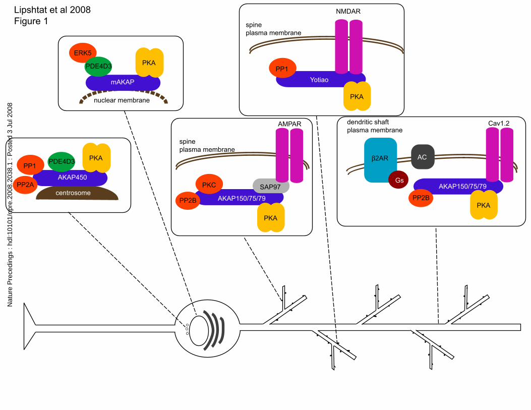
Fig 1 depicts the spatial segregation of PKA-interacting proteins and respective

substrates that is not captured in classical interaction graphs. In figure 1,-several PKA-

containing complexes with different subcellular localizations are shown. In each case

PKA interacts with a different version of the scaffold protein (A-kinase anchoring

protein, AKAP) which in turn binds other signaling components such as protein kinases,

phosphatases or channels. Most PKA found in the cell is bound to its scaffold protein

AKAP (10). In addition to the tethering of PKA, AKAPs are able to bind to a number of

other proteins, such as kinases or phosphatases, creating signaling hubs (11). There have

Nat

ure

Pre

cedi

ngs

: hdl

:101

01/n

pre.

2008

.203

8.1

: Pos

ted

3 Ju

l 200

8

6

been over 20 AKAP genes identified thus far and through the use of splicing the actual

number maybe closer to 50 AKAP-type proteins (10). Each AKAP has a specific

targeting domain that gives rise to differing localization within the cell (10), allowing for

the spatially distinct allocation of PKA signals along with its respective signaling

partners. This spatial segregation of a protein kinase and its substrates constitutes a

mechanism that promotes specificity of signaling by restricting the number of possible

downstream targets. In the example with PKA, distinct patterns of associations are seen

in various subcellular locations (Figure 1). This type of spatial information needs to be

accurately captured in network representations.

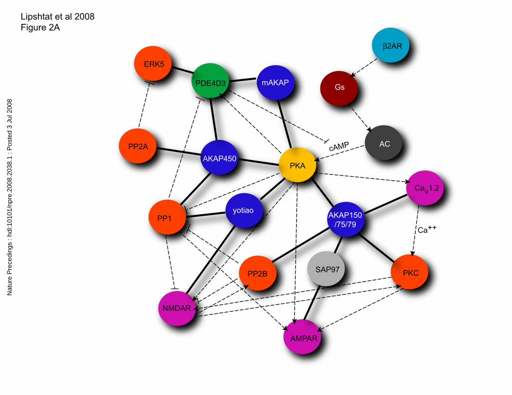
If one were to ignore spatial specification and only consider chemical interactions, we

can construct the classical CIG for protein kinase A interactors shown in Figure 2A. This

chemical interaction graph contains three types of interactions: the non-directional

scaffolding interaction, the directed arrows (activation), and directed plungers

(inhibition). All of the binary interactions in this graph have been experimentally

validated and hence we could consider the graph to be a correct representation of the

PKA network. This however is not the case. The protein kinase A chemical interaction

graph in Fig 2A implies distal relationships that are not correct if one takes into account

the spatial segregation of protein kinase A provided by the differential distribution of

AKAPs and its binding partners. For example, AKAP450 is localized to the centrosome

(12, 13) and is able to bind, along with protein kinase A, the phosphatases PP1 and PP2A,

and the phosphodiesterase PDE4D3 (14). There has been reports of PKA

phosphorylating PDE4D3-and PP1 dephosphorylating it and given their mutual

association to AKAP450 this is highly probable. A splice variant of AKAP450 is the

AKAP Yotiao (15). Yotiao is localized in neurons to their postsynaptic densities in

spines, where it forms a complex with the NMDA receptor (15). This splice variant still

retains the PP1 binding site but lacks the ability to bind PDE4D3 (16). Even though

AKAP450 and Yotiao share PP1 as a binding partner, due to their different subcelllular

locations, it is unlikely that that the two pools of PP1 will have the same local substrates.

Hence, the AKAP450 complex should not be connected to the Yotiao complex- since,

due to spatial constraints it is highly unlikely that any functional connections between

Nat

ure

Pre

cedi

ngs

: hdl

:101

01/n

pre.

2008

.203

8.1

: Pos

ted

3 Ju

l 200

8

7

these two complexes occur. Thus, NMDA or AMPA receptors and PDE4D3 are unlikely

to compete for either PKA or PP1 at a local level and more importantly PDE4DE is not

likely to locally regulate PKA control of NMDA receptors or AMPA channels through

the degradation of cAMP . Similarly from the graph in Figure 2A we could hypothesize

that protein kinase A, by regulating calcium channels (Cav1.2) (17), could modulate

protein kinase C (PKC) phosphorylation of the AMPA receptor channels (AMPAR) (18).

However this is not correct since calcium channels are in the dendritic shaft membranes

while AMPA receptor channels that give rise to the excitatory postsynaptic potential are

in the post synaptic densities in spines. These two examples illustrate the erroneous

inferences regarding connectivity and regulation one can arrive at from graphs that do not

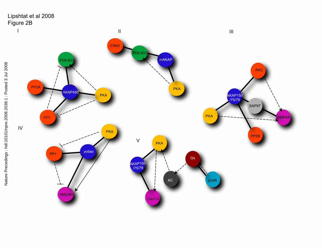
include spatial information. The subnetworks, shown in Fig 2B, take into account the

spatial specification of components and highlight how AKAPs function as location-

specific signaling hubs. From this description we can conclude that whereas the standard

CIG representation provides information regarding the possibility of a particular reaction

occurring it cannot tell us if the reaction will occur , as co-localization of reactants is a

requirement for the reaction to occur. Thus to draw valid functional inferences from

graphs of regulatory networks it is necessary to include spatial information.

Incorporating Spatial Specification into Graphs

Including spatial information into a graph that depicts a regulatory signaling network can

be done in one of two approaches. In cases where different compartments can be

physically defined (such as organelles such as the nucleus, or a subcellular compartment

such as cytoplasm, soma, dendrite, etc.) one may modify the network to include

compartment as part of a the name of a node. For example, instead of having a single

node to represent proteins such as MAP-Kinase 1, 2, one can have two separate nodes –

one for nuclear MAPK and one for cytoplasmic MAPK. The two nodes may be

connected by a link, representing the translocation event (19). This approach allows

certain reactions to be assigned exclusively to the nuclear MAPK species, such as

phosphorylation the nuclear kinase MSK(20) , without affecting the cytoplasmic MAPK,

which may have its own specific substrates such as cytoplasmic phospholipase-A2 (21).

Nat

ure

Pre

cedi

ngs

: hdl

:101

01/n

pre.

2008

.203

8.1

: Pos

ted

3 Ju

l 200

8

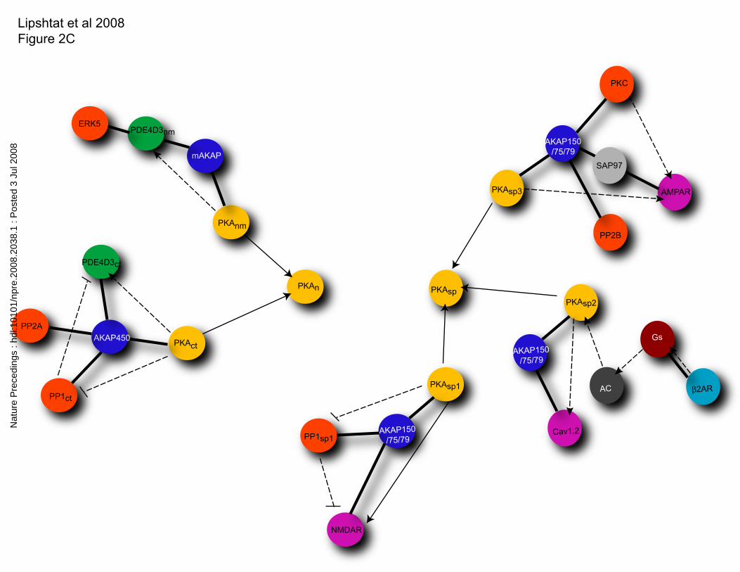
8

Applying this approach to the PKA network is shown in Figure 2C. Such modified

networks can be analyzed using any of the methods described above.

A different approach is to include detailed spatial information in the definition of nodes.

This is a natural extension of the ODE method. Instead of associating each node with a

time dependent concentration, the system is modeled by a set of partial differential

equations (PDEs) and each node represents a time and space dependent concentration.

Here there is no need to define compartments, as exact cartesian coordinates are included

in the concentration definition, and reactions take place only if all the respective reactants

are present simultaneously at the same coordinates. A limitation of this type of

representation is the loss of topological information that is essential for the identification

of motifs. Simulation of coupled-PDEs usually requires extensive computational

resources and is currently impractical for large-scale systems.

One can use the spatial distribution information to construct a new graph where spatial

information is used to specify the links. There are cases where experiments reveal spatial

distribution and localization of various cellular components. This data can be processed

into a network in the following manner: for each pair of components, calculate the

correlation coefficient between their respective spatial distributions. The correlation

coefficient between concentrations )(1 rρ and )(2 rρ is given by

21

21212,1 σσ

ρρρρ ∫∫∫∫ −=

dAdAdAdAC

where )()( 22iii EE ρρσ −= is the standard deviation and the integration is over the

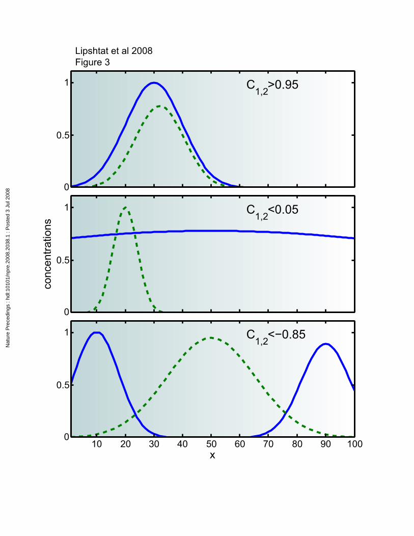
whole space. 2,1C is a measure of the overlapping between )(1 rρ and )(2 rρ (Figure 3).

The spatial correlation (C1,2) measures the extent to which distribution of component 1

may provide information and serve as a predictor to distribution of component 2. High

correlation between components 1 and 2 implies similar localization of the two

components. Areas with high concentration of 1 are expected to have also high

concentration of 2, and in locations where 1 is absent, 2 cannot have significant

concentration, either. Thus, it is enough to measure one of the components at a certain

Nat

ure

Pre

cedi

ngs

: hdl

:101

01/n

pre.

2008

.203

8.1

: Pos

ted

3 Ju

l 200

8

9

region in order to get good estimation of the two concentrations at that place (Figure 3A).

Low correlation is an indication to independent distributions (Figure 3B). When one of

the components (e.g. 1) is localized at a particular region, whereas the other component

(2) has a broad distribution, their correlation is low. In such a case, knowing the

concentration of 1 at a particular point doesn't increase our knowledge about 2, and vice

versa. It should be noted that such low correlation does not necessarily imply a lack of

interaction, since a locally concentrated component may be able to interact with a widely

distributed component. (C1,2) may get negative values as well. Negative correlation

(known also as anti-correlation) is a predictive tool just as the positive correlation.

However, in cases of negative correlation, high concentration of 1 at a particular location

indicates that 2 is expected to be absent from that region, and low concentration of 1

indicates high concentration of 2 (Figure 3C). Here again, like in the high correlation

cases, it should be enough to measure one component in order to gain information about

local concentrations of the two components.

Consider the case where we would link any two components whose correlation

coefficient is above an user defined threshold (for example 0.8). The resultant graph is

the spatial co-localization graph (SCG). In the protein kinase A example shown in Figure

1, the scaffold proteins Yotiao and AKAP450 will not be connected in a SCG although

they are closely related in the chemical interaction graph. An SCG can be analyzed using

conventional Graph theory metrics to find clusters and pathways which may indicate

critical intracellular areas and routes. More importantly, the SCG can be used as a filter

for the chemical interaction graph. The two graphs have the same set of nodes

(representing intracellular components). In most cases, only pairs of components that are

linked in both graphs have fulfilled the requirements for interaction from the biochemical

and the spatial criteria. This way the spatial information filters out interactions which are

possible biochemically but do not occur in a particular instance due to lack of

colocalization between interacting components.

Current experiments as yet do not provide data sets of localization of intracellular

components that allows us to construct an intracellular SCG. Thus in the system

Nat

ure

Pre

cedi

ngs

: hdl

:101

01/n

pre.

2008

.203

8.1

: Pos

ted

3 Ju

l 200

8

10

described in figure 1 , we know where individual components are localized, thse are from

different studies. So to illustrate the spatial co-localization graph, we have analyzed the

data of Petyuk et.al (22). This study describes the spatial distributions of over than 1000

proteins in the brain. It should be emphasized that this study does not include subcellular

localization, but rather tissue level distribution. Nevertheless, this is the first study that

describes such detailed spatial distribution on a large scale. There are ongoing efforts to

conduct high throughput imaging of intracellular proteins (23), but these large-scale

datasets are not yet publicly available. From the Petyuk et al study, we downloaded the

distributions of all the available proteins, and calculated the correlations between any pair

of them. Most of the proteins are well localized, indicating their concentrations are non-

zero in a defined region of the brain, and zero in the rest of the other regions. About 1/3

of the proteins had positive concentrations throughout the whole brain, indicating they

are broadly distributed components. Despite their low correlation with all other

components, these proteins can, chemical specificity permitting, interact with any other

protein irrespective of the spatial distribution. To examine the effect of the broadly

distributed components on the SCG we performed our analysis twice – once with all

proteins, including those that have a wide distribution, albeit at varying levels and again

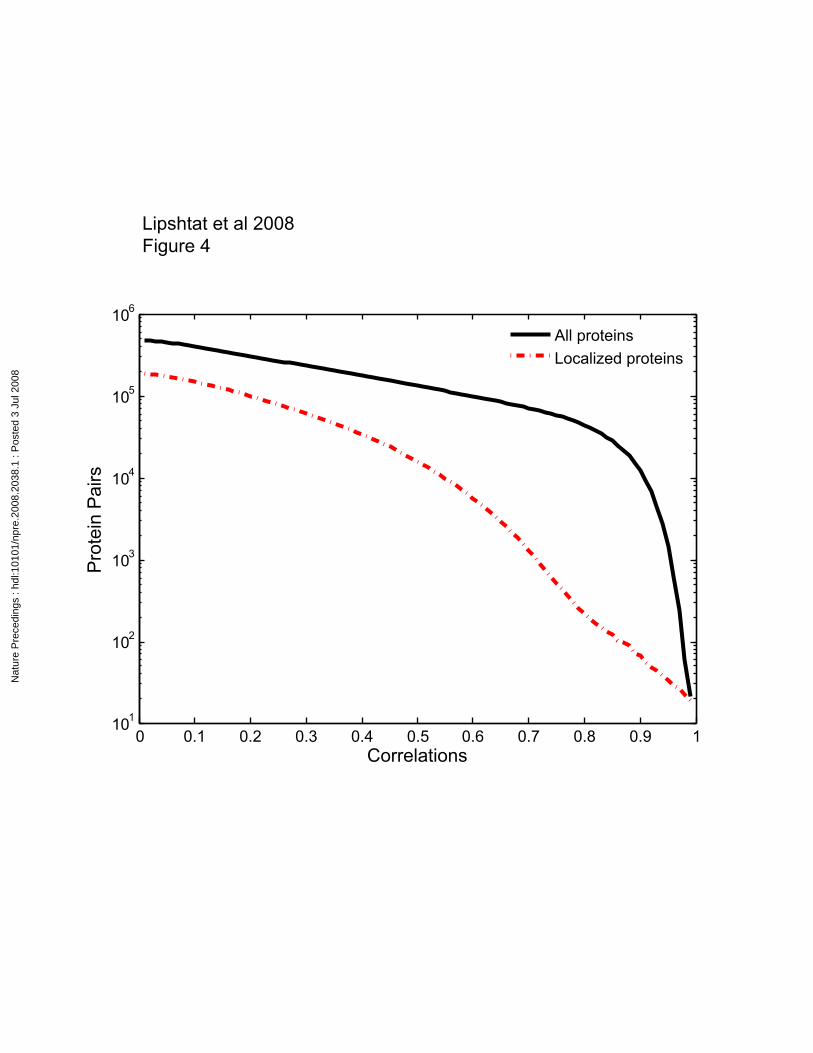
with only the localized proteins. The number of protein pairs (i.e. specification of links),

whose correlation is greater than a certain threshold is presented as function of the

threshold in Figure 4. When considering the whole data set (including the widely

distributed proteins), the number of links decreases exponentially with the threshold, until

the value of 0.8. Beyond that point there is a dramatic drop in the number of protein pairs

with higher correlation. This sharp change is not seen in the respective plot relating

exclusively to localized proteins (dashed plot in Figure 4). This difference indicates that

within the subset of widely distributed proteins, the typical correlation is in the range of

0.8-0.95. At the very high correlation range (C1,2>0.9) the difference between the two

plots gets smaller, and they coincide at the end (C1,2=1). Interestingly, there are about 20

pairs of proteins that are 99% correlated, and these proteins are all well localized.

The SCG provides a new tool for understanding cellular regulation. As a threshold has to

be determined while constructing the SCG, different threshold values produce different

graphs and provide different information respectively. For example, taking a very high

Nat

ure

Pre

cedi

ngs

: hdl

:101

01/n

pre.

2008

.203

8.1

: Pos

ted

3 Ju

l 200

8

11

threshold would result in the graph only component pairs that are localized together in a

very small region such as the 99% correlation described above. This high correlation

indicates tight co-localization and thus indicates either a physical compartment, like

nucleus, or common scaffold which is shared by the two correlated components. Even if

there is no evidence for mutual chemical affinity between such tightly correlate

components the spatial correlation can direct us to look for interactions, both direct and

indirect ones, that may be mediated through scaffolds or anchoring components. Spatial

correlation can also help to understand the functional role of a known chemical

interaction. As mentioned above, correlation can be either positive or negative (Fig. 3).

Whereas positive correlation indicates that the two components are co-localized and with

appropriate chemical specificity an interaction will occur, negative correlation is an

indication of the presence of one component and absence of the other. If the components

have the chemical ability to interact with one another, defining a negative threshold and

leaving only pairs of components whose correlation is below that threshold, gives us a

graph in which each link may predict a regulatory locus, where the movement of a

component is used to control chemical interaction and thus achieve local control of a

subcellular process. Such regulation can be either direct or indirect. The exact pathway

between the negatively correlated components would be found in the chemical interaction

data that specifies binary interaction capabilities, but the functionality of such a pathway

would be revealed by the differential spatial distribution.

However, considering spatial distribution by itself can result in erroneous representation

of the system. This error arises from the fact that some cellular components may be

broadly distributed, and nevertheless interacts with locally concentrated components.

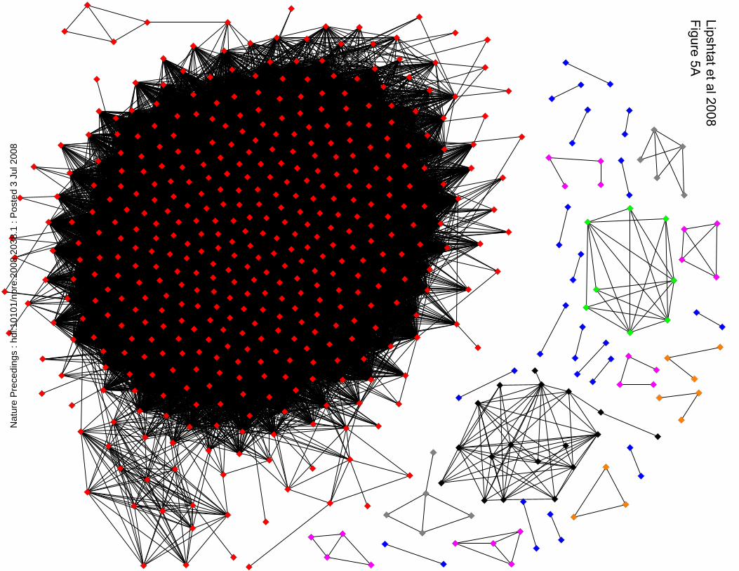
This situation can be seen by the analyses of the data of Petyuk et al. Using a threshold

of 0.8, yields a graph consisting of 532 nodes (proteins) and about 44000 links (pairs of

proteins with higher correlation than the threshold) (Figure 5A). The high density of links

in the major island in this graph arises from the high correlation of the widely distributed

components. This overwhelming connectivity obscures any meaningful information

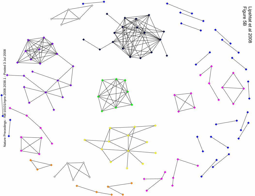
which may emerge from this graph. If the SCG in Figure 5A is filtered by considering

only co-localized proteins then the system is reduced to 224 links between 142 proteins

Nat

ure

Pre

cedi

ngs

: hdl

:101

01/n

pre.

2008

.203

8.1

: Pos

ted

3 Ju

l 200

8

12

(Figure 5B). However, from visual inspection of Figure 5B it can readily be seen that the

system is no longer a network but a set of isolated islands. This view is also not correct

since it is likely that some of the broadly distributed proteins will interact with some of

the local proteins and thus give rise to a better connected network rather that a set of

islands. Thus the systems visualized in Figures 5A and 5B represent two extremes of the

application of the spatial specification criteria and neither are realistic representations.

Taking the system in Figure 5A, if we eliminate the links where mutual chemical affinity

makes the interactions infeasible then we would obtain a much less densely interactive

network. Such analyses is not wholly feasible for the Petyuk et al data since this is tissue

not cellular localization, however the framework for mixed graphs where both

localization information and mutual chemical affinity are used to specify links are

described using a toy system.

Mixed graphs: understanding cellular regulation by analysis of spatial correlation

graphs integrated with chemical interaction graphs

Both chemical specificity and co-localization of the reactants are necessary conditions for

a reaction to occur. Thus, it makes sense to construct a multi-layer graph, where two

components are connected only if both conditions are fulfilled. However, as

demonstrated in Figure 5, the non-localized, widely distributed components require

special treatment. These components, chemical specificity permitting, may interact with

other components even if their respective correlation is low. Hence, the multilayered

graph has to include the widely distributed components with all their chemical specificity

links (regardless of spatial correlation), and the localized components whose links are

only those links that are present in both the spatial and chemical interaction graphs. A toy

example is presented in Figure 6. This example consists of 10 components, of which 5

are widely distributed (blue nodes, numbers 1 through 5) and the other 5 are localized

(red nodes 6-10). The SCG consists of all possible links between the non-localized

components, in addition to some co-localizations of well localized components (Figure

6A). Drawing the SCG solely for the localized components, yields a non-informative

graph (Figure 6B). The chemical specificity constraints are given by the CIG (Figure 6C).

For constructing the mixed graph we would like to combine the SCG with the CIG in the

Nat

ure

Pre

cedi

ngs

: hdl

:101

01/n

pre.

2008

.203

8.1

: Pos

ted

3 Ju

l 200

8

13

following way: for the widely distributed components (blue nodes 1-5) we take all of the

CIG links. However, between the localized components (nodes 6-10) we consider only

links which exist both in the SCG and in the CIG. Thus, for example, links (3 to 9) and (4

to 9) which do not appear at the SCG will be included at the final graph, since they

connect non-localized components (3 and 4, respectively). Interaction between

components 6 and 7 (or 7 and 10) is possible biochemically, however, since the two

reactants are not co-localized, these interactions should be excluded from the

multilayered graph (Figure 6D). Similarly, components 8 and 9 are co-localized, but in

that case the lack of chemical specificity prevents them from interacting. The resulting

mixed graph (Figure 6D) provides an integrative information which is represents a more

accurate picture of all the interactions within the system than the CIG or the SCG by

themselves. Such a mixed graph can be used for both steady state analysis and dynamical

simulations. For dynamic simulations, the correlation coefficient associated with each

link can be used as a multiplicative factor altering the overall rate (i.e. concentration of

reactants X the kinetic rates) to yield “effective” reaction rates. This reflects the fact that

for any given pair of reactants, only the correlated fraction of each reactant can be

involved in the reaction and not the entire pool, which may be located at many other

places. This way the spatial information can not only affect the topology of the network

but also the dynamics of the various components.

Perspective

Recent studies in our laboratory have shown that the dynamics of locally elevated

concentrations of signaling components depends on the topology of the interaction

network within which these components function (24). Signal transmission through

regulatory networks not only involves information regarding the activity state of the

component but also information about the location of the active component. This type of

study based on partial differential equation is very useful in understanding the spatial

dynamics of key signaling component and how spatial information is transmitted from

upstream to downstream components with a given pathway or network. However the

role of network topology, especially the location of network motifs both in the chemical

Nat

ure

Pre

cedi

ngs

: hdl

:101

01/n

pre.

2008

.203

8.1

: Pos

ted

3 Ju

l 200

8

14

interaction space as well as subcellular location is not easily deduced from such studies.

For this both the CIG and SCG are needed. Hence approaches that allow for facile Graph

theory based computation of mixed CIG and SCG will be very useful in understanding

and predicting complex cellular regulation

Acknowledgements:

This research was supported by NIH grants GM 072853 and DK-038761 and the Center

for Systems Biology

Nat

ure

Pre

cedi

ngs

: hdl

:101

01/n

pre.

2008

.203

8.1

: Pos

ted

3 Ju

l 200

8

15

References

1. Strogatz, S. H. 2001 Exploring complex networks. Nature 410:268-276. 2. Bollobás, B. 1998. Modern Graph Theory. Graduate Texts in Mathematics, vol. 184, Springer, New york.

3. Barabási,A.-L. and R. Albert. 1999. Emergence of Scaling in Random Networks. Science 286:509-512.

4. Watts, D. and S. Strogatz. 1998. Collective dynamics of 'small-world' networks. Nature 393: 440-442.

5. Alon, U. 2003. Biological Networks: The Tinkerer as an Engineer. Science, 301:1866-1867.

6. Ma’ayan, A. et al. 2005. Formation of regulatory patterns during signal propagation in a mammalian cellular network. Science 309:1078–1083. 7. Bromberg, K.D., A. Ma’ayan, S.R. Neves, and R. Iyengar. 2008. Design logic of a cannabinoid receptor signaling network that triggers neurite outgrowth. Science, in press. 8. Lipshtat, A., S.P. Purushothaman , R. Iyengar, and A. Ma'ayan. 2008. Functions of Bifans in Context of Multiple Regulatory Motifs in Signaling Network. Biophys J. 94:2566-2579. 9. Milo, R., S. Shen-Orr, S. Itzkovitz, N. Kashtan, D. Chklovskii, and U. Alon. 2002. Network Motifs: Simple Building Blocks of Complex Networks. Science 298:824-827. 10. Michel, J.J, and J.D. Scott. 2002. AKAP mediated signal transduction. Annu Rev Pharmacol Toxicol 42:235-257. 11. Smith, F.D, L.K. Langeberg, J.D. Scott. 2006. The where's and when's of kinase anchoring. Trends Biochem Sci 31:316-323. 12. Takahashi M, H. Shibata, M. Shimakawa, M. Miyamoto, H. Mukai, and Y. Ono. 1999. Characterization of a novel giant scaffolding protein, CG-NAP, that anchors multiple signaling enzymes to centrosome and the golgi apparatus. J Biol Chem 274:17267-17274. 13. Witczak O, B.S. Skalhegg, G. Keryer, M. Bornens, K. Tasken, T. Jahnsen, S. Orstavik. 1999. Cloning and characterization of a cDNA encoding an A-kinase anchoring protein located in the centrosome, AKAP450. Embo J 18:1858-1868. 14. Tasken KA, P. Collas, W.A. Kemmner, O. Witczak, M. Conti, and K. Tasken. 2001. Phosphodiesterase 4D and protein kinase a type II constitute a signaling unit in the centrosomal area. J Biol Chem 276:21999-22002.

Nat

ure

Pre

cedi

ngs

: hdl

:101

01/n

pre.

2008

.203

8.1

: Pos

ted

3 Ju

l 200

8

16

15. Lin, J.W., M. Wyszynski, R. Madhavan, R. Sealock, J.U. Kim, and M. Sheng. 1998. Yotiao, a novel protein of neuromuscular junction and brain that interacts with specific splice variants of NMDA receptor subunit NR1. J Neurosci 18:2017-2027. 16. Westphal, R.S., S.J. Tavalin, J.W. Lin, N.M. Alto, I.D. Fraser, L.K. Langeberg, M. Sheng, and J.D. Scott. 1999. Regulation of NMDA receptors by an associated phosphatase-kinase signaling complex. Science 285:93-96. 17. Hall D.D., M.A. Davare, M. Shi, M.L.Allen, M. Weisenhaus,G.S. McKnight, J.W.Hell. 2007. Critical role of cAMP-dependent protein kinase anchoring to the L-type calcium channel Cav1.2 via A-kinase anchor protein 150 in neurons. Biochemistry 46:1635-1646. 18. Tan SE, R.J. Wenthold, and T.R. Soderling. 1994. Phosphorylation of AMPA-type glutamate receptors by calcium/calmodulin-dependent protein kinase II and protein kinase C in cultured hippocampal neurons. J Neurosci 14:1123-1129. 19. Chen RH, Sarnecki C, Blenis J. 1992. Nuclear localization and regulation of erk- and rsk-encoded protein kinases.Mol Cell Biol. 1992 Mar;12:915-27 20. Deak M, A.D. Clifton, L.M. Lucocq, and D.R. Alessi.1998. Mitogen- and stress-activated protein kinase-1 (MSK1) is directly activated by MAPK and SAPK2/p38, and may mediate activation of CREB.EMBO J. 17:4426-41. 21. Lin LL, M. Wartmann, A.Y. Lin, J.L. Knopf, A. Seth, and R.J. Davis.1993.cPLA2 is phosphorylated and activated by MAP kinase.Cell. 72:269-78. 22. Petyuk, V.A., W-J. Qian, M.H. Chin, W. Haixing, E.A. Livesay, M.E. Monroe, J.N. Adkins, N. Jaitly, D.J. Anderson, D.G. Camp, II, D.J. Smith, and R.D. Smith. 2007. Spatial mapping of protein abundances in the mouse brain by voxelation integrated with high-throughput liquid chromatography-mass spectrometry. Genome Res. 17: 328-336. 23. Kai, H. and R. Murphy. 2004. Boosting accuracy of automated classification of fluorescence microscope images for location proteomics. BMC Bioinformatics, 5:78. 24. Neves S. R., .Tsokas P., Sarkar A., Grace E. A.,, Rangamani P., Taubenfeld S. M.m alberini C. M., Schaff J. C. Blitzer R. D., Moraru I. I. and Iyengar. R ( 2008) Cell shape and negative links in regulatory motifs together control spatial information flow in signaling networks Cell in press

Nat

ure

Pre

cedi

ngs

: hdl

:101

01/n

pre.

2008

.203

8.1

: Pos

ted

3 Ju

l 200

8

17

Figure Legends

Figure 1

Schematic representation of the subcellular localization of protein kinase A (PKA)

interacting proteins in a neuron. This schematic figure shows how due to presence of

different isoforms of the scaffolding protein different combinations of PKA interacting

proteins are colocalized in different regions of the neuron. The abbreviations are as

follow: kinases- protein kinase A, PKA, extracellular regulated kinase 5, ERK5 and

Protein kinase C, PKC; A-kinase anchoring proteins AKAPs- AKAP450, mAKAP,

AKAP150/75/79 and Yotiao (AKAP9); Phosphatases- protein phosphatase 1, PP1,

protein phosphatase 2A PP2A and protein phosphatase 2B, PP2B; and Phosphodiesterase

PDE4D3; ionic channels- alpha-amino-3-hydroxy-5-methylisoxazole-4-propionic acid

receptor, AMPAR, N-methyl-d-aspartate receptor, NMDAR and L-type Calcium channel

Cav1.2. Receptor- beta-adrenergic receptor, β2AR; heterotrimeric G protein Gs;

Adenylyl Cyclase AC

Figure 2

Protein kinase A interaction networks in neurons A. Protein kinase A-centric protein-

protein interaction network without considering localization. Physical interactions are

depicted as solid lines. Functional interactions are depicted as dashed arrows. The

functional interactions represent enzymatic reactions, conformational changes or non-

proteinacious intermediates. B. Subnetworks that result from consideration of spatial

localization resulting from localization localization of AKAPs to different regions of the

neuron. C. Inclusion of compartment ID as part of the definition of a node.

Abbreviations for compartments are as follow: ct centrosome, nm nuclear membrane, n

nucleus, sp spine. Please note that there may be a great deal of heterogeneity in the

protein composition of each spine. Thus we have sub classified spines into spine1,

spine2 and 3 to capture this.

Nat

ure

Pre

cedi

ngs

: hdl

:101

01/n

pre.

2008

.203

8.1

: Pos

ted

3 Ju

l 200

8

18

Figure 3

Demonstration of spatial correlations in a schematic one dimensional cell.

Concentrations are normalized to the range from 0 to 1 and space is labeled x and varies

from 0 to 100. For example this could 1 to a 100 microns within a cell. A. High

correlation – the two components are localized at t same area.. Presence (absence) of one

component is a good marker for presence (absence) of the other. B. Low correlation –

data regarding one component cannot provide any indication to presence or absence of

the other. C. Negative correlation – presence (or absence) of one component indicates

absence ( or presence) of the other.

Figure 4

Number of component pairs whose correlation is greater than a given threshold, as

function of the threshold. Localized proteins are defined as proteins with zero

concentration at least in one area of the brain as shown by Petyuk et al (22). 20 pairs of

proteins have correlation >0.99.

Figure 5

Spatial correlation graph of the data obtained from Ref. 22, with a threshold 0.8. The

colors indicate size of clusters. A. SCG of the whole data. 532 nodes and >44000 links

are organized in one large cluster of 433 nodes (in red), one cluster of 18 nodes (black),

one cluster of 8 nodes (green) and 2, 5, 3, and 17 clusters of size 5, 4, 3, and 2

respectively (gray, pink, orange, and blue). B. SCG of the same data used in Figure 5A

after removing the broadly distributed components. Total of 142 nodes and 224 links in

single clusters of sizes 20, 18, 13, 8 each (purple, black, yellow, green, respectively.) and

2, 7, 3, and 18 clusters of size 5, 4, 3, and 2 respectively (gray, pink, orange, and blue).

Figure 6

Demonstration of the steps in building a mixed graph. This toy example consists of 5

widely distributed components (in blue) and five localized components (in red). A. The

complete SCG. The widely distributed components are highly connected (similar to the

Nat

ure

Pre

cedi

ngs

: hdl

:101

01/n

pre.

2008

.203

8.1

: Pos

ted

3 Ju

l 200

8

19

big island in Figure 5A). B. Spatial correlation of the localized components alone (similar

to Figure 5B). C. The chemical interaction graph (CIG). D. The mixed graph consists of

all the links connected to blue nodes in the CIG (panel C) plus the links which appear

both in the SCG and the CIG (intersection of panels B and C). An edge between two

nodes in this graph indicates that interaction between the respective two components can

occur due to both chemical specificity and spatial co-localization.

Nat

ure

Pre

cedi

ngs

: hdl

:101

01/n

pre.

2008

.203

8.1

: Pos

ted

3 Ju

l 200

8

PKAPDE4D3

ERK5

mAKAP

nuclear membrane

PKAPDE4D3

AKAP450

centrosome

PP1

PP2A

PKA

AKAP150/75/79

PKC

PP2B

AMPAR

PKA

YotiaoPP1

NMDAR

spineplasma membrane

Lipshtat et al 2008Figure 1

SAP97

PKA

AKAP150/75/79

PP2B

Cav1.2

β2AR AC

Gs

spineplasma membrane

dendritic shaftplasma membrane

Nat

ure

Pre

cedi

ngs

: hdl

:101

01/n

pre.

2008

.203

8.1

: Pos

ted

3 Ju

l 200

8

PKA

mAKAPPDE4D3

ERK5

PP1

PP2AAKAP450

AMPAR

AKAP150/75/79

PKCPP2B

yotiao

NMDAR

SAP97

Cav1.2

Gs

β2AR

ACcAMP

Ca++

Lipshtat et al 2008Figure 2A

Nat

ure

Pre

cedi

ngs

: hdl

:101

01/n

pre.

2008

.203

8.1

: Pos

ted

3 Ju

l 200

8

PKA

PP1yotiao

NMDAR

PKA

mAKAP

PDE4D3

ERK5

PKA

PDE4D3

PP1

PP2AAKAP450

PKA AMPAR

AKAP150/75/79

PKC

PP2B

SAP97

AKAP150/75/79

Cav1.2

Gs

β2ARAC

PKA

I II III

IV

V

Lipshtat et al 2008Figure 2B

Nat

ure

Pre

cedi

ngs

: hdl

:101

01/n

pre.

2008

.203

8.1

: Pos

ted

3 Ju

l 200

8

PKAnm

mAKAP

PDE4D3nmERK5

PKAct

PDE4D3ct

PP1ct

PP2AAKAP450

PKAn

PKAsp1

PP1sp1

NMDAR

PKAsp3 AMPAR

AKAP150/75/79

PKC

PP2B

SAP97

AKAP150/75/79

Cav1.2

Gs

β2ARAC

PKAsp2

AKAP150/75/79

PKAsp

Lipshtat et al 2008Figure 2C

Nat

ure

Pre

cedi

ngs

: hdl

:101

01/n

pre.

2008

.203

8.1

: Pos

ted

3 Ju

l 200

8

conc

entra

tions

0

0.5

1

x10 20 30 40 50 60 70 80 90 100

0

0.5

1

0

0.5

1

C1,2<−0.85

C1,2<0.05

C1,2>0.95

Lipshtat et al 2008Figure 3

Nat

ure

Pre

cedi

ngs

: hdl

:101

01/n

pre.

2008

.203

8.1

: Pos

ted

3 Ju

l 200

8

0 0.1 0.2 0.3 0.4 0.5 0.6 0.7 0.8 0.9 1101

102

103

104

105

106

Correlations

Pro

tein

Pai

rs

All proteinsLocalized proteins

Lipshtat et al 2008Figure 4

Nat

ure

Pre

cedi

ngs

: hdl

:101

01/n

pre.

2008

.203

8.1

: Pos

ted

3 Ju

l 200

8

Lipshtat et al 2008Figure 5A

Nat

ure

Pre

cedi

ngs

: hdl

:101

01/n

pre.

2008

.203

8.1

: Pos

ted

3 Ju

l 200

8

Lipshtat et al 2008Figure 5B

Nat

ure

Pre

cedi

ngs

: hdl

:101

01/n

pre.

2008

.203

8.1

: Pos

ted

3 Ju

l 200

8

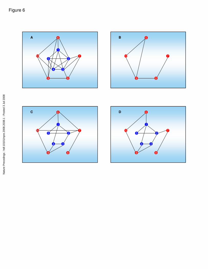
Figure 6

1

5 2

4 3

6

10 7

9 8

A 6

10 7

9 8

B

1

5 2

4 3

6

10 7

9 8

C

1

5 2

4 3

6

10 7

9 8

D

Nat

ure

Pre

cedi

ngs

: hdl

:101

01/n

pre.

2008

.203

8.1

: Pos

ted

3 Ju

l 200

8