rural adjustment assistance -...
TRANSCRIPT

Rural Adjustment Assistance Assessment and
options
ABARE Submission to Senate Standing Committee on Rural
and Regional Affairs
June 1994
m
e ABARE

Foreword
In March 1994 the Senate Standing Committee on Rural and Regional Affairs
announced that it would be undertaking an inquiry into the Rural Adjustment Scheme.
The focus of the inquiry is on the adequacy of the scheme in meeting present and future
needs of producers, the extent of rural debt and the roles for government, industry and
the financial sector in rural adjustment.
Rural adjustment assistance has been changed a number of times over the past two
decades, with the latest change being introduced on 1 January 1993. In its annual
broadacre farm survey conducted in 1993, ABARE collected information relating to
farms applying for RAS, in addition to the normal physical and financial information
which is collected each year. This provides a statistical database for making some
preliminary assessments of the performance of the latest RAS.
In this submission consideration is also given to the justifications for government
intervention in rural adjustment and possible future directions of government policy. In
particular, if farmers have effective mechanisms to manage risks, this should enable a
reduced reliance on government assistance in the future and a more efficient farm
sector.
BRIAN FISHER
Executive Director, ABARE
June 1994

Acknowledgments
This submission was prepared in the Agriculture and Natural Resources Group of
ABARE. The project was supervised by Paul Morris and Vivek TulpuM. The principal
contributors (in alphabetical order) were Phil Kokic, Lynelle Moon, Paul Morris,
Bhamathy Parameswaran, Deborah Peterson, Stephen Strachan, Vernon Topp,
Elizabeth Toussaint, Vivek Tulpul6 and Jane Wright. Assistance and input was also
provided by Stephen Beare and John Hempton.

Contents
Summary
1 Introduction
2 Background Origins of RAS
Current provisions of RAS
3 Financial position of Australian farms Importance of the rural sector in the Australian economy
Financial characteristics of broadacre and dairy farms
Rates of return
4 Role of government in provision of assistance to the rural sector Social welfare
Efficiency arguments
Other risk management policies
Interest subsidies
5 Characteristics of Rural Adjustment Scheme applicants Farm performance characteristics
Off-farm assistance measures
Future equity positions of RAS and non-RAS farms
Summary of assessment
6 Future directions for rural adjustment
Appendices A Assumptions used in farm equity analysis
B Tax averaging, income equalisation deposits and farm management
bonds
References

Figures 1 Farm cash income and farm business profit for broadacre farms
2 Debt servicing ratio: non-RAS farms vs new RAS farms
3 Farm cash income: non-RAS farms vs new RAS farms
Tables 1 Financial performance measures
2 Distribution of farms, by debt
3 Financial performance by receipt class
4 Characteristics of broadacre farms, 1992-93
5 Broadacre farms receiving off-farm assistance, 1992-93
6 New RAS recipients - equity position after five years
7 Old RAS recipients -equity position after five years
8 Non-RAS applicants -equity position after five years
Box Income tax averaging, income equalisation deposits and farm management
bonds 44

Summary
On 24 March 1994 the Scnatc rcquested that the Senate Standing Committee on Rural
and Regional Affairs undertake an inquiry into the Rural Adjustment Scheme (RAS). In
this submission focus is placed on the justifications for and adequacy of RAS to meet
the needs of the rural sector.
It is important to recognise that most farmers do not receive RAS and effectively
manage their own financial and other risks. Around 10 per cent of farms have received
assistance since 1 January 1993 (when the new RAS came into force), with more than
half of these receiving assistance under the exceptional circumstances provisions and
around one-third receiving assistance under the skills enhancement program.
The new RAS Commonwealth government involvement in rural adjustment extends back to at least
1935. Rural adjustment assistance has undergone a number of changes over this period.
The current RAS, which took effect on 1 January 1993, is directed toward assisting
farmers to become more sclf-reliant with respect to farm risks. In the present schemes
greater emphasis than in the past, is being placed on assisting farmers who have a high
probability of being profitable in the long run, and on sustainability and productivity of
the farm sector. It is intended that the RAS (at least in its present form) will come to an
end in the year 2000.
Some of the instruments used under the new RAS remain similar to the previous
scheme. For example, assistance continues to be provided in the form of interest
subsidies of up to 50 per cent on commercial finance to farmers facing short run
difficulties and re-establishment assistance of up to $45 000 to assist farmers whose
farms are unviable to leave the sector.
The main changes in the new RAS included:
moving some of the social welfare aspects of the old RAS into a new Farm
Household Support Scheme;
establishing an exceptional circumstances provision which provides up to 100 per
cent interest subsidies to farmers in temporary severe difficulties due to an
exceptional event such as major drought or flood;

establishing a farm purchase program to enable State authorities to enter into land
transactions;
establishing a skills enhancement program to assist farmers to improve their
business skills;
placing a greater emphasis on farm productivity, profitability and sustainability
rather than on assistance and debt reconstruction as under the old scheme; and
providing adjustment assistance for groups of farmers to improve productivity,
profitability or sustainability at the regional level (recent government
announcements indicate that the Sunraysia region of Victoria will be the first to
have RAS funds specifically targeted to regional needs).
Farm performance Many parts of the rural sector have been suffering from depressed incomes for the past
four years. This has been the result of low world prices for some major agricultural
commodities (in particular, wool) and adverse seasonal conditions in some states. There
is some evidence of an improvement in income over the past two years. For example,
average farm cash income for the broadacre sector increased by 18 per cent in 1992-93
(albeit from relatively low levels), with a further increase of 33 per cent expected in
1993-94.
Nevertheless, around 25 per cent of broadacre farms are expected to have negative cash
flows in 1993-94, with around 36 per cent of farms in the sheep specialist industry
expected to suffer cash losses. Average debt levels also remain high in some parts of the
farm sector. Real average debt levels have only fallen to $126 300 per farm in 1993-94
compared with the peak of $136 000 per farm in 1986-87 (in 1993-94 dollars).
Moreover, in 1992-93 the proportion of income expended in making interest payments
on debt was around 31 per cent on average for broadacre farms, and around 60 per cent
for the sheep industry. However, about 31 per cent of farms were estimated to cany no
debt at 30 June 1993, and average equity levels remain high at around 86 per cent.
Farm performance also varies substantially by size of farm. Results from analysis of
farm survey data indicate that in all broadacre industries there is a clear pattern of
increasing rates of return as farm size increases. For example, in 1992-93 in the wheat
and other crops industry, the average rate of return for small farms (those with less than
$200 000 in receipts) was -0.6 per cent, compared with 7.8 per cent for large cropping
farms (those with greater than $400 000 in receipts). This divergence between rates of
return should encourage commercially based adjustment in farm size, capital value or
other relevant factors so that rates are similar across farms. The ultimate extent of this
adjustment could be substantial given the large proportion of small farms in each
industry.
However, there are a number of reasons why adjustment does not occur, some of which
are commercially based, while others represent impediments to efficient adjustment
(some of which are discussed below). As an example of commercial factors, some land
values, which form a large percentage of total capital and are high (on a per hectare
basis) for the small farms, are heavily influenced by proximity to large urban centres,
and so may reflect factors over and above the return from use of the land for agriculture
(such as the expected capital appreciation if the land were to be sub-divided for urban
expansion in the future). At the same time, small farms have a high level of plant and
machinery capital per area cropped, and this may reflect over-capitalisation or
economies of scale from expanding area. It is important to distinguish between normal
market factors and impediments to adjustment in determining the appropriate role for
government. Further research is required into the relative importance of such influences
and on the factors determining the differences in returns earned by different size farms.
Comparison of RAS applicants pre- and postJanuary 1993 ABARE has undertaken preliminary analysis to consider the extent to which the new
RAS (introduced on 1 January 1993) achieves its objectives of directing assistance to
more financially viable farms. The results obtained, while based on only one year's data,
appear to be consistent with the conclusion that new RAS farms are in a better financial
position than those receiving RAS in the six months prior to 1 January 1993. At this
early stage of the new RAS it is more difficult to assess the extent to which other
objectives (such as increased self-reliance) are being achieved.
Justifications for intervention Governments intervene in the rural sector for a range of reasons. These reasons can be
categorised as foIlows:
Welfare
Governments intervene to adjust the distribution of income across segments of the
community to improve the welfare of those in financial difficulty or in poverty.
Similarly, the isolation of some regions makes access to alternative employment

opportunities and to training more difficult, and farmers near retirement may be
reluctant to move and start a new career. Government assistance for social welfare
purposes could be through direct payments or through the provision of services
(such as communication and access to education and training). In providing such
assistance it is important that income is redistributed in a manner which does not
cause significant distortions in the allocation of resources.
Efficiency
Governments also intervene to improve the operation of the market where it is
expected that the market acting alone will not provide an efficient allocation of
resources. This may be as a result of markets failing to exist for some goods or
services, markets failing to provide information, the existence of physical
externalities (off-site impacts) or the market resulting in erratic adjustment which
may create large adjustment costs.
Arguments under each of these categories can and have been used to justify various
assistance provisions under RAS. There are several instruments under RAS, of which
some could be interpreted as addressing efficiency concerns, such as exceptional
circumstances, or as addressing a mixture of welfare and efficiency concerns, such as
the re-establishment program, the skills enhancement program and subsidies on interest
payments.
It is important that the government apply instruments which are appropriate to
addressing specific existing problems, with, potentially, a different instrument being
applied to each problem. Whether these instruments are placed in RAS or other policy
frameworks is largely a question of administrative efficiency.
The revisions to RAS which took effect in 1993 transferred household support, a major
welfare component of the old RAS, to the Farm Household Support Act 1992 which is
delivered on an agency basis by the Department of Social Security. As noted, there still
remain some elements of RAS which have a social welfare component. In delivering
these remaining welfare elements, the principal efficiency concerns are cost
effectiveness and any links between eligibility requirement or payments which impede
desired social or economic adjustment. At present, RAS authorities are closely involved
in the relationship between individual clients and the commercial lending sector and
may be in the best position to continue to administer some forms of welfare assistance.
From an administrative sense it may therefore be efficient that RAS continues to
contain both social welfare and efficiency elements.

An important motivation for government intervention is the absence or inadequacy of
existing markets. For example, insurance markets presently do not cover certain
extreme events, such as drought and flood. In the absence of such markets, extreme
events could result in a significant exodus of farmers from particular regions. Such exits
and re-entry can impose costs on society. RAS exceptional circumstance provisions
provide some limited assurance against such risk.
Exceptional circumstances provisions also apply to price risks. The argument that other
industries have access to markets which agriculture lacks do not apply as readily here.
For example, futures markets are available for a range of agricultural commodities. For
other commodities, government policies to protect farmers against price risks may have
impeded the development of risk markets. For example, the operation of the Reserve
Price Scheme for wool may have impeded the development of forward wool markets.
However, the removal of many such schemes from the agricultural sector suggests
farmers will be required to manage price risks in a similar fashion to other industries.
Hence, there is not a strong case for exceptional circumstances assistance to continue to
be applied to price risks.
The government also provides other instruments which farmers can use to manage
income flows. For example, income equalisation deposits (IEDs) and taxation
provisions provide means for farmers to smooth tax payments and adjust income flows.
Provisions covering income averaging, depreciation and tax credits can have a
substantial effect on investment margins on-farm and within the management unit of
the farm enterprise. However, there are a number of possible changes to IEDs which
would make them more attractive to farmers. In particular, improvements are needed to
the tax treatment of IEDs to enable interest earned to be taxed at a rate more closely
aligned with individual farmers' marginal tax rates.
Another motivation for government intervention is the role it plays in providing public
information through education and training. Training grants are available under RAS to
assist farmers in learning how to manage financial and market risks. The current
objective of RAS to increase self-reliance in the farm sector is partly addressed through
such training programs which may be seen as an ongoing aspect of rural education. The
question about whether RAS is an appropriate vehicle to deliver such services rests
largely with the cost effectiveness of delivery. At present, the federal and state RAS
authorities may be in a good position to identify educational need, direct clients to
appropriate providers and to administer funding. In the longer term, it may be more

efficient to meet any additional need for farm business and technical training through
the rural education system.
The government may also have a role in addressing the significant land degradation and
environmental problems which are affecting productivity and profitability of the farm
sector. In particular, this role stems mainly from the external effects of private land
management decisions on other farmers and other members of the community.
Remedies to some environmental problems need to be undertaken at both the farm and
community levels. For example, the benefits from introducing drainage works to
address rising water tables are likely to accrue to a number of farms in a region.
The use of instruments under RAS in combination with other programs, such as
Landcare, may be able to address some of these problems. For example, the skills
enhancement program may be used to improve farmers sustainable farming skills. The
government may also have a role in purchasing seriously degraded land and retiring it
from agriculture. Such provisions may be able to be used as an alternative to re-
establishment grants, which require the farm to be sold and may simply perpetuate land
degradation problems.
However, it is likely that governments will need to apply instruments other than those
within RAS to more directly address some of the land degradation problems facing
some rural areas. For example, adoption of appropriate water pricing, widely tradable
water entitlements and economically efficient decisions on infra-structure replacement
could substantially improve the efficient use of water and sustainable agricultural
practices in the Murray-Darling Basin and other areas of Australia. Such policies may
also increase the rate of adjustment in irrigation areas. To the extent that such
adjustment creates social welfare problems there may be scope for some intervention to
address these problems. Again, it is important that such social welfare policies do not
distort the adjustment which is necessary in these regions. Re-establishment grants and
re-training assistance may be useful in this regard.
Related to this, it may be cost effective for government to attempt to accelerate or retard
the rate of adjustment more generally, where the rate of adjustment which would
otherwise occur would impose costs on other parts of society. For example, the costs of
providing the social welfare services associated with any large scale capital
restructuring of Australian agriculture may be lower if the restructuring occurs
smoothly as opposed to catastrophically. Alternatively, the government can also speed
adjustment where necessary. Re-establishment grants and land purchase provisions can

assist the orderly exit of the least viable farmers from agriculture. Similarly, exceptional
circumstance provisions may act to limit adjustment in temporary periods of adversity.
However, the existence of such provisions may limit required adjustment in periods of
exceptionally good prices or seasonal conditions.
Future directions
Governments have a number of general objectives for the rural sector, including
attaining profitable, productive and sustainable farming across Australia. The future for
farmers, as with other industries, rests with all farmers adopting financial, risk and
farming management practices which ensure they are efficient in the long term. This
will enable a substantial reduction in the role of government in rural adjustment in the
future. The removal of some elements of RAS assistance would mean that all farmers
would be responsible for managing their own risks (recognising that most farmers
currently do this).
Effective risk management requires that farmers have access to the necessary skills and
instruments to manage the various risks that they face. There already exists a large
number of means by which farmers can manage their risks. These include insurance
markets (for normal risks), futures markets and on-farm management measures (such as
various drought strategies). There are also some income modification mechanisms
which help farmers manage their tax liabilities or smooth their incomes - such as
income equalisation deposits (IEDs), farm management bonds (FMBs) and tax
averaging. An important role for government is ensuring that the instruments it provides
to assist farmers in this regard are effective and efficient. The change to the tax
treatment of IEDs suggested above would assist in achieving this.
There is not a strong argument for continuation of interest subsidies for farmers, nor for
exceptional circumstances as applied to price risks. There is a question about whether
interest subsidies are the most appropriate means of facilitating adjustment in that they
target adjustment only through borrowings. There are a range of more appropriate
instruments which directly assist the adjustment of agriculture, such as re-establishment
grants and land trading, and those which assist farmers during extreme adverse
circumstances due to natural diasters, such as parts of the exceptional circumstances
provisions. There is also a case for improved government policies with respect to the
irrigation sector, including more efficient water pricing and increased water tradability.
Assistance for training and for regional adjustment are consistent with broader
government objectives in terms of provision of public information and addressing
public good problems associated with the environment. While the role of RAS
compared with other policy frameworks can be considered, there is a case for some
continued government involvement.
Finally, it needs to be borne in mind that the need for rural adjustment arises from a
variety of sources and for a variety of reasons. In most cases, adjustment will occur in
the absence of intervention. Governments therefore need to target their efforts at
removing impediments to efficient adjustment and at the social welfare consequences of
adjustment. It is unlikely that any one instrument or policy, such as RAS, will address
all of these concerns. Rather instruments should be chosen to target specific problems
and should be placed within government to achieve maximum administrative efficiency.

1. Introduction
On 24 March 1994 the Senate requested that the Senate Standing Committee on Rural
and Regional Affairs undertake an inquiry into the Rural Adjustment Scheme and report
by the first sitting day in October 1994. More specifically, the terms of reference given
to the Standing Committee were:
(a) the adequacy of the Rural Adjustment Scheme, including its current guidelines
and operation, in meeting the present and future needs of primary producers
suffering from prolonged adverse circumstances beyond their control;
(b) the extent of rural debt, the nature and serviceability of that debt and its social,
economic and ecological consequences; and
(c) what mechanisms should be recommended for the management of rural
reconstruction and the contributing roles of government, the financial sector and
industry.
In this submission focus is placed on the justifications for and adequacy of the Rural
Adjustment Scheme (RAS) to meet the needs of the rural sector. RAS provides
assistance to only a limited proportion of Australian farms. For example it is estimated
that around 10 per cent of farms have received assistance since 1 January 1993 (when
the new RAS came into force), with more than half of these receiving assistance under
the exceptional circumstances provisions and around one-third receiving assistance
under the skills enhancement program (DPIE submission to Senate Inquiry). This
means that most farmers are self-reliant in managing risks. To demonstrate this, in this
submission background material is provided on the current performance of the rural
sector, including the distribution of performance within the sector. This draws on data
collected by ABARE in its surveys of Australian farms.
Arguments which have been used to justify RAS assistance are then critically discussed.
In this regard it needs to be remembered that the objectives of RAS have changed over
time and are now focused on helping farmers become more self-reliant and on assisting
farmers with a higher probability of viability in the long run. A preliminary assessment
of the performance of the new RAS in achieving the latter objective is provided in the
submission. Finally, some discussion is provided of possible future directions for the
RAS and other risk management instruments.

2. Background
A brief summary of the origins and features of the Rural Adjustment Scheme (RAS) is
provided in this section. More detailed background on the origin and current
components of RAS has been provided to the Standing Committee in the submission by
the Department of Primary Industries and Energy.
Origins of RAS
RAS has its origins in a number of schemes established in the early 1970s, although
Commonwealth government involvement in rural adjustment dates back to at least
1935. The first of the more recent schemes, the Marginal Dairy Farms Reconstruction
Scheme, was established in 1970. This was followed by the Rural Reconstruction
Scheme in 1971, the Fruitgrowing Reconstruction Scheme in 1972 and the Dairy
Adjustment Program (replacing the former dairy scheme) in 1974. The Dairy
Adjustment Program was then revised in 1976. In 1977, following an Industries
Assistance Commission inquiry, the Rural Adjustment Scheme was established,
replacing all former schemes.
RAS applied to all agricultural, horticultural, pastoral, apicultural and aquacultural
industries, and was established to administer three types of assistance;
Part A Adiustment Assistance. The federal government provided concessional
funds to the state rural adjustment authorities for lending to applicants.
Part B Cam-on Assistance. The state and federal governments provided joint
funds for carry-on assistance.
Part C Household Su~port . The federal government provided loans for up to three
years to fund living expenses. The loan could be converted into a grant if the
farmer left the farm within that time.
Since 1977, RAS has been revised several times following reviews by the Industries
Assistance Commission (in 1984 which resulted in changes to RAS introduced in
1986), Coopers and Lybrand WD Scott (which resulted in the 1988 RAS) and Synapse
Consulting (Aust) Pty Ltd (which formed the basis for the new RAS which was enacted
in 1992 and came into force on 1 January 1993). While maintaining the broad structure
of the 1977 scheme until 1992, RAS has gradually evolved to more accurately reflect

the different needs and circumstances surrounding the farm, finance and government
sectors. For example, in 1986, the process for implementing adjustment and carry-on
assistance was altered from direct payments to interest subsidies. In 1988, the emphasis
of RAS shifted toward those farmers with long term prospects of profitability and with
financial difficulties beyond their control.
In 1992, the categories A, B and C were abolished. Whereas previous schemes had
focused on assistance and debt reconstruction, the new scheme is concentrated under a
single program, with the focus on farm productivity. The household support component
of the scheme was moved from the RAS framework. Household support is now
provided under the Farm Household Support Scheme, and is serviced by the
Commonwealth Department of Social Security on an agency basis.
In the second reading speech for the Rural Adjustment Bill 1992, the then Minister for
Primary Industries and Energy stated that '... it is intended that the Scheme will be
reviewed after four years and will come to an end after eight years'. The objective at the
time was to establish a farming sector which was able to grow and respond to market
and environmental conditions without the need to rely on government assistance. As a
consequence the new RAS was directed toward assisting farmers to become more
effective risk managers. Emphasis was placed on assisting those farmers having a high
probability of being viable in the long run, while not impeding the necessary adjustment
out of the industry of those farmers not likely to be viable.
Current provisions of RAS
The current provisions of RAS are contained in the Rural Adjustment Act 1992. There
were also a number of initiatives announced in the government's Working Nation White
Paper released in May 1994. The main features of RAS as it currently stands are
summarised below.
50per cent interest subsidy
Fanners facing financial difficulties are able to access interest rate subsidies of up to 50
per cent on the cost of commercial finance, to enhance further productivity and
profitability of their businesses (these can be used for purposes such as adopting new
technology, improving resource use, improving farm programs or adopting sustainable
farming practices).

Exceptional circumstances
Farm businesses suffering severe financial hardship as a result of exceptional
circumstances (such as severe drought or severe price downturn) can access interest
subsidies of up to 100 per cent under thc exceptional circumstances component of RAS.
The Minister for Primary Industries and Energy must determine that an exceptional
circumstance exists before farms can apply, and, to qualify, farm businesses must be
profitable in the long term and have access to commercial finance (with interest
subsidies).
Re-establishment assistance
RAS currently provides a re-establishment grant to eligible farmers leaving the farm
sector. A grant of up to $45 000 is available subject to income and assets tests to
farmers on the sale of their productive assets.
Training
Farmers may be eligible for grants for training to upgrade farm business management
skills and to assist with the cost of obtaining financial planning and other professional
advice relating to the farm business.
Special Farm Purchase Program
State Authorities have the capacity within RAS to enter into transactions in order to
acquire, hold and dispose of land and aquacultural holdings to facilitate improvements
in farm performance or to facilitate the orderly exit from the industry for farmers
without prospects.
Regional assistance
The 1992 RAS included a provision for groups of farmers to seek adjustment assistance
to improve productivity, profitability or sustainability. These groups could be classified
by industry or by region. As part of the Working Nation package (Prime Minister,
1994), the Sunraysia region is the first to have RAS funds targeted to the specific needs
of the region, a precedent likely to be extended to other regions in the near future.
Liltking RAS to other programs
As part of the Working Nation package, RAS is to be reviewed to ensure better linkages
to other programs including the Agribusiness and Landcare programs (Prime Minister
1994). This focus is to be in conjunction with the re-direction toward regional
assistance.

3. Financial position of Australian farms
Demands for assistance to the rural sector are often based on arguments related to the
importance of maintaining the contribution of the sector to the Australian economy and
the impact of the decline in agricultural terms of trade on the financial position of many
Australian farmers. The agricultural sector has declined in importance to the overall
state of the Australian economy over recent decades. It is apparent that for a range of
market and, in some cases, environmental reasons many farmers are facing severe
financial difficulties. At the same time, there are many farmers who consistently receive
moderate to high returns from their farming activities.
Importance of the rural sector in the Australian economy
The contribution of agriculture to gross production in Australia is relatively low and has
been declining over time. The rural sector directly contributed 3.2 per cent of GDP in
1992-93 as compared to 26 per cent of GDP in 1950-51 (ABARE 1993). Comparing
this with other sectors, in 1992-93 wholesale and retail trade contributed 18 per cent of
GDP and manufacturing contributed to 15 per cent of GDP. Similarly, agriculture
employs 406 000 people or 5 per cent of the labour force, compared with 21 and 14 per
cent of the labour force employed by wholesale and retail trade and manufacturing
respectively (ABARE 1993). Of course agriculture also indirectly contributes to
employment and production in other associated industries.
Despite low contributions to GDP, agriculture remains an important export industry. In
1992-93, farm output contributed 21 per cent of the total value of Australian exports.
However, again the farm share in total exports has been declining with farm export
income making up 85 per cent of total export income in 1950-51 (ABARE 1993).
Australia is a relatively small supplier of most agricultural commodities on world
markets (the principal exception being wool). Therefore, Australia often has little
influence on market prices for agricultural commodities, which are characterised by
volatility. World prices are often distorted by agricultural policies in other major
agricultural trading nations. For example, in 1992 the rate of assistance (as measured by
the producer subsidy equivalent) for Australia was calculated at 12 per cent compared
with an OECD average of 44 per cent (OECD 1993).
In addition to variations in prices, farmers also have had a declining terms of trade - that is the ratio of an index of prices received for outputs and prices paid for inputs. The

index of farmers' terms of trade (1987-88 = 100) has fallen from 252 in 1951-52 to 82 in
1992-93 (ABARE 1993). This has meant that farmers have continually needed to
increase productivity in order to remain economically viable. Between 1971-72 and
1988-89, productivity growth in the rural sector was estimated to be 2.7 per cent a year.
By comparison, over the period 1968-69 to 1988-89 the manufacturing sector was
estimated to have productivity growth of 1.7 per cent a year (Males, Davidson, Knopke,
Loncar and Roarty 1990).
Variations in output as a result of environmental influences exacerbate income
fluctuations faced by farmers (Males, Davidson, Knopke, Loncar and Roarty 1990).
Some of these environmental influences only affect income in the short run- for
example, rainfall variations; however, there are longer term environmental changes
which will affect the profitability of farming in Australia over the coming decades.
According to the CSIRO about 52 per cent of Australia's agricultural and pastoral land
have been degraded to the extent to which they are now in need of significant recovery
action (CSIRO Institute of Natural Resources and Environment 1990). However,
increasing recognition of this problem by farmers and governments is resulting in some
moves to reduce the causes and effects of degradation. In a recent survey of Australian
broadacre farmers ABARE found that 28 per cent of farmers perceived a problem with
water erosion, 20 per cent had a problem of woody weed spread while 16 per cent
perceived dryland salinity to be a problem on their property (Mues, Roper and Ockerby
1994). It was also found that 49 per cent of farmers claimed a tax deduction related to
expenditure on conserving or conveying water, and controlling or preventing land
degradation.
Financial characteristics o f broadacre and dairy farms
The Australian farm sector has been suffering relatively low incomes for the past four
years (figure 1). This has been the result of low world prices for some major agricultural
commodities (in particular, wool) and adverse seasonal conditions in some states
(particularly Queensland and parts of New South Wales). There has been some
turnaround in returns to rural producers in the past two years. For example, based on
information collected from ABARE's annual survey, in the broadacre farm sector
average farm cash income (defined as total cash receipts less total cash costs) increased
by 18 per cent in 1992-93 with a further increase of 33 per cent expected in 1993-94.

Figure 1: Farm cash income and farm business profit for broadacre farms Average per farm
In 1993-94 dollars 80000
Farm cash income
This is in part the result of an improvement in the world economy but also because
many of Australia's agricultural and pastoral regions experienced their second
successive year of good to excellent seasonal conditions. In contrast, large areas of
Queensland were subjected to drought which severely limited both crop and livestock
production.
Farm cash income is estimated to have risen for all the broadacre industries and for the
dairy industry in 1993-94. As can be seen in table 1, the largest percentage increases are
expected for the sheep and sheep-beef industry but this increase is from an extremely
low base. For the sheep industry, an estimated 36 per cent of farms are expected to
continue to face a farm cash loss in 1993-94, compared with 25 per cent for broadacre
agriculture overall and 4 per cent for the dairy industry.
Farm business profit is an approximate measure of net funds available for investment
generated by the farm enterprise. It is a measure of the gains from farming after
allowance has been made for: the value, calculated at award rates, of the labour input
reported for each proprietor and family member; the notional run-down or depreciation
in the value of plant and improvements; and the value of the buildup or rundown in
inventories of stock or produce held on-farm over the year.

Table 1 . Financial performance measures Averages per farm
All broadacre Wheat and other croos 1991-92 1992-93,, 1993-94, 1991-92 1992-93p 1993-94s
Total cash receipts $ 139 916 152 750 155 800 218680 314450 306800
Total cash costs $ 116282 124820 118500 157 105 228590 217900 Farm cash income $ 23 633 27 930 37 200 61 575 85 860 89000 Farms with positive farm cash income % 70 Farm business profit $ -24 701 Farms with positive farm business profit % 19 Profit at full equity a $ -8 218 Capital appreciation $ -3 202 Profit at full equity b $ -1 l 419 Farm capital at 30 June $ 924 5 15
Farm debt at 30 Junee $ 122 219 Change in debtc $ 6311 Equity at 30 .hn'?d $ 772 099 Equity ratioe % 86.3 Debt servicing ratiof % 37.7
Rate of return a % -0.9 Rate of returnb % -1.2 Real rate of returnb % -3.1
1991-92 1992-93p 1993-94,
Total cash receipts $ 182 005 178 780 184 400 Total cash costs $ 145 089 138 020 135 000 Farmcash income $ 36916 40760 49 500 Farms with positive farm cash income % 8 1 82 8 1 Farm business profit $ -18 893 -10 310 -3 100 Farms with positive farm business profit % 24 31 30 Profit at full equitya $ 1 192 4680 11000 Capital appreciation $ 17 530 11 940 na Profit at full equity b $ 18 722 16 620 na F m capital at 30 June $ 866 099 823 230 na Farm debt at 30 Junee $ 140 683 138 970 134 800 Change in debtc $ 6320 4750 -3100 Equity at 30 Juned $ 698 675 663 630 na Equity ratioe % 83.2 82.7 na Debt servicing ratiof % 3 1.4 24.4 19.2 Rate of return a % 0.1 0.6 1.3 Rate of return b % 2.2 2.0 na
Sheer, 1991-92 1992-93p 1993-94,
102 378 92 380 94 700 97 087 84920 80400
5291 7460 14300
Real rate of returnb % 0.3 1 .o na -5.4 -5.2 na
continued on next page

Table I (continued) Beef Sheeo-Beef
1991-92 1992-93p 1993-94s 1991-92 1992-93p 1993-94)4,
Total cash receipts $ 1 18 275 149 240 150 700 111762 111230 118400 Total cash costs $ 99 093 126260 1 I6 500 99660 100190 93400 Farm cash income $ 19 183 22 980 34 300 12102 11040 25000 Farms with positive
farm cash income % 66 70 75 62 68 76 Farm business profit $ -21 325 -17 970 -3 200 -34 692 -28 520 -9 000 Farms with positive farm business profit % 19 29 38 12 16 27 Profit at full equitya $ -9 028 -5 310 7 800 -18600 -14340 3 300 Capital appreciation $ -24 3 17 10 480 na -14623 -12030 na
Profit at full equity b $ -33 344 5 170 na -33222 -26360 na
Farm capital at 30 June $1 051 612 1 188 650 na 985092 927190 na
Farm debt at 30 Junee $ 95 674 l l l 030 109 300 124572 124550 117600 Change in debtc $ 7 227 6 950 -400 11279 11310 -700 Equity at 30 Juned $ 892 100 991 120 na 843 182 790520 na
Equity ratioe % 90.3 89.9 na 87.1 86.4 na Debt servicing ratiof % 36.7 31.9 21.9 54.6 52.6 30.3 Rate of return a % -0.8 -0.5 0.7 -1.8 -1.5 0.4 Rate of return b % -3.1 0.4 na -3.3 -2.8 na
Real rate of returnb % -5.0 -0.6 na -5.2 -3.8 na
Dairv 1991-92 1992-93p 1993-94,
Total cash receipts $ 156 621 173 290 181 600 Total cash costs $ 112220 118090 114900 Farmcashincome $ 44401 55210 66700 Farms with positive
farm cash income % 94 97 96 Farm business profit $ -2 028 12 310 18 500 Farms with positive farm business profit % 40 Profit at full equitya $ 14 665 Capital appreciation $ 14 894 Profit at full equity b $ 29 559 Farm capital at 30 June $ 892 405 Farm debt at 30 Junee $ 105 156 Change in debt e $ 4415 Equity at 30 Juned $ 788 330 Equity ratioe % 88.2 Debt servicing ratiof % 22.7 Rate of return a % 1.7 Rate of return b % 3.4
Real rate of return b % 1.5 7.4 na
a Excluding capital appreciation. b Including capital appreciation. c Average per responding farm. For assistance in interpreting estimates of debt, see 'Survey methods and definitions'. d Total farm capital minus total farm debt. e Equity expressed as a percentage of total farni capital. f Interest paid divided by the sum of interest and farm cash income. p Preliminary estimate. s Provisional estimate. na Not available.

Average broadacre farm business profit, while still expected to be negative in 1993-94
(figure 1 and table I), is estimated to show an improvement of 66 per cent. This is in
part attributable to a marked increase in the value of buildup in trading stocks,
particularly cattlc, comparcd with 1992-93.
Around 31 per cent of broadacre farms are estimated to earn a positive farm business
profit in 1993-94, compared with 26 per cent in 1992-93. There is considerable
diversity across the broadacre industries, with average farm business profit expected to
be negative in 1993-94 for all industries except the wheat and other crops industry.
While farm business profit is only an approximate financial measure, it is fair to
conclude that farm returns have not been sufficient to maintain investment levels in
broadacre agriculture as a whole over the past four years.
The average farm debt for broadacre farms rose steadily in real terms from 1978-79, to
a peak of $136 000 in 1986-87. By 30 June 1993, average broadacre farm indebtedness
had fallen only slightly to $133 140 (in 1993-94 dollars). Average broadacre debt is
estimated to have fallen by 1 per cent to $126 300 per farm in 1993-94.
Across the broadacre industries, the estimated change in average debt ranges from an
increase of $6600, or 3 per cent, in the wheat and other crops industry, to a fall of
$3100, or 2 per cent in the mixed livestock-crops industry (table 1). The declining
average debt and negative farm business profit are associated with a net decline in the
capital base of broadacre agriculture. This may be appropriate if either there was over-
capitalisation in agriculture, or if the relative cost of capital versus other inputs has
changed.
The level of debt varies considerably across farms as shown in table 2. About 34 per
cent of broadacre farms are expected to carry no debt at the end of 1993-94. This
compares with an estimated 31 per cent of broadacre farms with no debt in 1992-93.
The highest proportion of debt-free farms is in the beef industry, where almost 41 per
cent of the population have no debt. In contrast, 13 per cent of all broadacre farms and
19 per cent of wheat and other crops farms are expected to have debts in excess of
$250 000 at the end of June 1994.
Despite a small increase in average farm indebtedness during 1992-93, average
broadacre farm equity remained at 86 per cent at the end of June 1993 (table 1). Equity
was highest in the beef industry at an average of 90 per cent. In the sheep industry
average equity fell by $19 350 per farm in 1992-93, as land values declined. Falls were
largest in the pastoral zone where production alternatives are limited.

Table 2: Distribution of farms, by debt At 30 June
Percentage of farms with debt equal to or below estimated value 1991-92 1992-93p 1993-94, 1991-92 1992-93p 1993-94,
$ $ $ $ $ $ Broadacre industries Wheat and other crons-
12.5 per cent 0 0 0 0 0 3 800 25.0 per cent 0 0 0 12 275 14 440 10000 50.0 per cent 35267 37600 37000 66816 92310 76300 75.0 per cent 148244 148410 140800 152257 223 610 204900 87.5 per cent 294531 293870 278000 340 490 413 170 382 200
12.5 per cent
25.0 per cent
50.0 per cent
75.0 per cent
87.5 per cent
12.5 per cent
25.0 per cent
50.0 per cent 75.0 per cent
87.5 per cent
Mixed livestock-cro~s Sheen
0 0 0 0 0 0 4 599 700 600 947 1440 700
69 389 58490 54 300 29628 26440 29200 209623 183 110 178800 155041 142410 129600 334003 333 160 312900 272 555 287 890 266 200
Beef Sheepbeef
0 0 0 0 0 0 0 0 0 0 0 0
13 295 25 050 26500 24 590 35 170 31 400 106101 112690 107200 143538 146620 138600 173 419 202 010 213 700 297 897 273 020 233 800
Dairv
12.5 per cent 0 0 0 25.0 per cent 12043 6420 8600 50.0 per cent 41 738 55670 58500 75.0 per cent 141 675 167 970 164 100 87.5 per cent 265 601 260 870 264 400
p preliminary estimate. s provisional estimate. na not available.
The average debt servicing ratio, the proportion of total income that is expended in
making interest payments on farm debt, rose to 39 per cent in 1990-91. Despite an
increase in average debt since that time, the debt servicing ratio has fallen sharply due
to the marked fall in interest rates. It is estimated that in 1992-93 the debt servicing ratio
averaged 31 per cent for broadacre farms. The debt servicing ratio in the sheep industry,
estimated at 60 per cent in 1992-93, was the highest among the broadacre industries.
Rates of return
In any one year, rates of return in agriculture vary substantially. For a variety of
reasons, differences occur across regions, and both within and across industries. Over

the longer term, however, rates of return in general should be similar, as capital is
attracted to industries or regions performing well (thereby increasing land values), or is
withdrawn from industries or regions performing poorly (leading to a reduction in land
values). As a result, rates of return should tend toward a common level.
Average rates of return derived from farm survey data are typically presented at an
industry or region level. As such they tend to illustrate prevailing price conditions
(industry level results), or the impact of seasonal conditions (region level results). To
gain an insight into how farms of different size are performing, average rates of return
have been calculated for three farm size categories in the wheat and other crops, sheep
and beef industries (table 3).
The results show a clear pattern of increasing rates of return as farm size increases. For
example, in the wheat and other crops industry, the average rate of return for small
farms (those receiving less than $200 000 in farm cash receipts) was -0.6 per cent in
1992-93, compared with 7.8 per cent for large farms (those receiving more than
$400 000 in receipts). However, in comparing across groups, it should be noted that
within each size category the top 25 per cent of farms earned considerably higher rates
of return than the bottom 75 per cent of farms, although the pattern of increasing returns
as farm size increased also held for the top performing farms within each group. This
overall pattern also appears to persist over time in most cases, as can be seen for 1985-
86 in table 3.
The adjustment process in agriculture at least in part, depends on the speed and efficacy
with which resources move into and out of industries as relative rates of return change.
Adjustment in this sense includes the process whereby existing farms expand in size to
take advantage of productivity and scale economies. At face value, the results
mentioned above suggest that structural adjustment should occur as smaller farms
earning low rates of return either invest in additional land or other capital to increase
their size and profitability, or are bought out by existing farms seeking to do likewise.
Even medium sized farms earning median level returns face similar incentives to
increase size and output to generate higher rates of return. However, as noted above, the
divergence in rates of return between small and large farms has been a feature of
broadacre agriculture in Australia for a considerable period. While average farm size
has been increasing, it has been at a relatively slow rate.

Table 3: Financial performance, by receipt class Average per farm Wheat and other crops industry Less than $200 000 $200 000 to $400 000 Greater than $400 000
Top 25 per cent Top 25 per cent Top 25 per cent Unit Average by rate of return Average by rate of return Average hy rate of return
1992-93 Area operated at30 June ha 59 1 469 1 344 1 183 3 199 3 218 Total area cropped ha 319 266 837 724 1 797 1 976 Rate of return % -0.6 7.9 4.3 11.5 7.8 17.3 Total closing capital $ . 615 580 581 850 847 650 723 860 1 854 900 1 330 200 1985-86 Rate of return % -2.87 2.83 1.53 16.74 2.21 9.18
Sheep industry Less than $100 000 $100 000 to $200 000 Greater than $200 000
Top 25 per cent Top 25 per cent Top 25 per cent Unit Average by rate of return Average by rate of return Average hy rate of return
1992-93 Area operated at 30 June ha 1 750 890 1 1 320 1 1 010 27 100 35 480 Sheep at 30 June no. 1 966 2 774 5 134 4 620 12 172 12 743 Rate of return % -6.5 0 -1.4 3.4 0.6 4.7 Total closing capital $ 578 360 1016 680 1056 990 1 002 250 2 239 030 2 022 650 1985-86 Rate of return % -3.04 1.45 -1.65 3.13 0.96 7.72
Beef industry (excluding major Less than $100 000 $100 000 to $200 000 Greater then $200 000 feedlots)
Top 25 per cent Top 25 per cent Top 25 pcr cent Unit Average by rate of return Averaze by rate of return Average by rate of rclurn
1992-93 Area operated at 30 June ha 3 760 1720 8 740 4 380 51 650 108 100 Beef cattle at 30 June no. 310 410 710 510 2 620 3810 Rate of return 9~ -4.1 1.6 -0. I 4.0 2.0 9 .9 Total closing capital $ 730 530 707 890 I 325 040 1 067 830 2 828 740 2 808 850 1985-86 Rate of return % -2.19 2.38 1.40 10.79 0.72 8.88

However, there are a number of reasons why adjustment does not occur, some of which
are commercially based, while others represent impediments to efficient adjustment
(some of which are discussed below). As an example of commercial factors, some land
values, which form a large percentage of total capital and are high (on a per hectare
basis) for the small farms, are heavily influenced by closeness to large urban centres,
and so may reflect factors over and above the return from use of the land for agriculture
(such as the expected capital appreciation if the land were to be sub-divided for urban
expansion in the future). Of course land values are also influenced by a range of other
factors, which may include the effects of government intervention.
At the same time, small farms have a high level of plant and machinery capital per area
cropped, and this may reflect over-capitalisation or economies of scale from expanding
area. Further research is required into the factors determining the differences in returns
earned by different size farms. It is important to distinguish between normal market
factors and impediments to adjustment in determining the appropriate role for
government. These impediments and the role for government in correcting them are
discussed in the next chapter.

4. Role of government in provision of assistance to the rural sector
Governments intervene in the rural sector for a range of reasons. These reasons can be
discussed in terms of social welfare and efficiency.
Arguments under each of these categories can and have been used to justify various
assistance provisions under RAS. There are several instruments under RAS, of which
some could be interpreted as addressing efficiency concerns, such as exceptional
circumstances, or as addressing a mixture of welfare and efficiency concerns, such as
the re-establishment program, the skills enhancement program and subsidies on interest
payments.
It is important that the government apply instruments which are appropriate to
addressing specific problems which exist, with, potentially, a different instrument being
applied to each problem. Whether these instruments are placed in RAS or other policy
frameworks is largely a question of administrative efficiency.
Social welfare
Governments often intervene to adjust the distribution of income across segments of the
community to improve the welfare of those in financial difficulty or in poverty. There
are a number of social reasons why adjustment may be slow in parts of the agricultural
sector. For example, the isolation of some regions makes access to alternative
employment opportunities and to training more difficult, and may require a farmer to
move to a large town or city. Moreover, the average age of broadacre farm operators in
1992-93 was around 53 years (ABARE farm survey data). Farmers close to the normal
retirement age may be reluctant to train for and move into new careers.
Government intervention for social welfare reasons takes a number of forms, including
through direct payments and the provision of services (such as communication and
access to education and training). Assistance can also take the form of subsidies on
particular goods and services or inputs into production. Such assistance can distort
production and consumption decisions and create losses to society. Therefore, in
providing social welfare it is important that consideration is given to the manner in
which income is redistributed to minimise significant distortions in the allocation of
resources.

The revisions to RAS which took effect in 1993 transferred household support, a major
welfare component of the old RAS, to the Farm Household Support Act 1992 which is
delivered on an agency basis by the Department of Social Security. As noted, there still
remain some elements of RAS which have a social welfare component. In delivering
these remaining welfare elements, the principle efficiency concerns are cost
effectiveness and any links between eligibility requirement or payments which impede
desired social or economic adjustment.
At present, RAS authorities are closely involved in the relationship between individual
clients and the commercial lending sector and may be in the best position to continue to
administer some forms of welfare assistance.
Efficiency arguments
Governments also intervene to improve the operation of the market where it is expected
that the market acting alone will not provide an efficient allocation of resources. This
may be as a result of markets failing to exist for some goods or services, markets failing
to provide information, the existence of physical externalities (off-site impacts) or the
market resulting in erratic adjustment which may create large adjustment costs.
Market existence
In general, market mechanisms should ensure that farmers adopt appropriate risk
management practices and adjust their behaviour in response to various market and
environmental pressures. For example, mixed enterprise farmers often adjust their
production mix in response to changes in returns from different products. In recent
years there has been a significant shift from sheep into cropping in response to the
change in relative prices from the two activities. Governments have a role in rural
adjustment in so far as they can, in a cost-effective manner, address problems which
sometimes arise in market determined adjustment. At the same time, as noted by
Musgrave (1985), the appropriate size and activities of government will be limited by
many factors including the effectiveness of any government policy if implemented.
While there appears to be little case on efficiency grounds for interest subsidies in the
main part of RAS, there may be some justification for subsidies under exceptional
circumstances provisions. The Australian rural sector has been characterised by
occasional disasters such as extended droughts, extreme floods or commodity price
crashes which have a very small probability of occurring in any one year but which
impose a significant (and perhaps overwhelming) cost when they do occur.

In most other industries some of these low probability but high loss events are catered
for through insurance markets. However, normal insurance markets have not catered
well for the agricultural sector with respect to natural disasters. The insurance industry
gives a number of reasons for the absence of an insurance market for such risks. These
reasons include: there 'must be a spread of risk by nature and location so that no single
event can cause a loss of such magnitude that it would eliminate the premium pool and
reservesp-and the 'events must be of a fortuitous nature and not influenced or capable of
being influenced by deliberate action on the part of the insured' (Cloney, p. 1994 p20).
Widespread exceptional droughts may fall into the first of these categories, while more
regular seasonal fluctuations, which farmers can not influence but can manage for, may
fall into the second category - 'Natural events like drought and flood are generally not
insurable risks since both are seen as a management risk and capable of some influence
by the farmer (eg fodder conservation)' (Cloney 1994, p. 20).
In the absence of insurance markets for these risks, exceptional droughts and floods
could result in a significant exodus of farmers from particular regions. Such exits, and
eventual re-entry, from the sector are not costless due to the transactions costs involved
and the fact that capital and labour are not perfectly mobile throughout the economy. If
it were expected that a consequence of such adjustment would be a more efficient farm
sector, then the adjustment costs may be worth bearing. However, where events are
truly exceptional, and existing farmers in the affected region are efficient over the
medium to long term, then such costs may impose a loss on society (for discussion of
the efficiency costs of farm foreclosures see Leathers and Chavas 1986).
Provided the full costs of the assistance (including costs associated with collection and
payment) are less than the loss from unnecessary adjustment in the farm sector, then
there may be a case on efficiency grounds for some government assistance for natural
disasters. At the same time, the full costs of providing such assistance needs to be
considered - including the distortionary and administrative costs associated with
collecting taxes from other sectors. Findlay and Jones (1982) indicate that for
Australian income taxes these distortions may be substantial.
While the above discussion has focused on natural disasters, exceptional circumstance
provisions also apply to commodity market downturns. The arguments used above with
regard to agriculture being disadvantaged relative to other industries due to the absence
of insurance markets are less applicable in the case of price declines. As in the
agricultural sector, businesses in other sectors are also often unable to insure themselves

against abnormal price declines. However, in some cases other markets do exist for
such risks. For example, futures markets are available for many agricultural
commodities and are extensively used by some producers. In particular, cotton growers
in Australia use a range of methods to protect themselves against adverse price
movements, including hedging on the New York Futures exchange and pooling of risks.
For other commodities, government policies to protect farmers against price risks may
have impeded the development of risk markets. For example, the operation of the
Reserve Price Scheme for wool may have impeded the development of forward wool
markets and some short term intervention may be required until such markets have had
adequate time to develop. Overall, however, the arguments for providing exceptional
circumstances assistance for price risks are not strong.
Information market failures
The government has a role in providing public information through education and
training. Training grants are available under RAS to assist farmers in learning how to
manage financial and market risks. The current objective of RAS to increase self
reliance in the farm sector is partly addressed through such training programs which
may be seen as an ongoing aspect of rural education. The question about whether RAS
is an appropriate vehicle to deliver such services rests largely with the cost effectiveness
of delivery. At present, the federal and state RAS authorities may be in a good position
to identify educational need, direct clients to appropriate providers and to administer
funding. In the longer term, it may be more efficient to meet any additional need for
farm business and technical training through the rural education system.
Existence of externalities
Over the past decade Australian governments have increased their emphasis on the
significant land degradation and environmental problems which are affecting the
productivity and profitability of the rural sector. For example, the introduction of the
Decade of Landcare program is specifically directed at forming community based
groups to deal with such problems. Similarly, the new RAS places increased emphasis
on providing assistance to address regional adjustment issues, some of which arise from
environmental problems.
The role for government in this regard arises mainly from the external effects of private
land management decisions - particularly those which are difficult to measure or
attribute to particular individuals (Morris, Wilks and Wonder 1992). Externalities
include reduced water quality for downstream users from soil erosion, chemical
outflows or saline discharge, rising water tables and consequent dryland salinity

problems, and movement of soil due to wind or water erosion creating damage to roads,
other farms or other activities. In the absence of government intervention there would
often be inadequate incentive for individuals to act to correct some of these problems - since the benefits of individual action largely accrue to other individuals while the costs
are internalised.
Remedies to some environmental problems, such as those mentioned above, often need
to be undertaken both at a community level and a farm level. For example, the benefits
from introducing drainage works to address rising water tables are likely to accrue to a
number of farms in a region, while the benefits of tree planting on farms are often farm
specific but do have some beneficial impact on other farms in a region. Therefore, a
regionally based adjustment program may be the most appropriate means of dealing
with these issues.
The use of instruments under RAS in combination with other programs, such as
Landcare, may be able to address some of these problems. For example, the skills
enhancement program under RAS could be partly directed toward new techniques and
management practices which assist in achieving sustainable farming practices. There
may be efficiency reasons for government intervention to coordinate problem solving
between interest groups when there are problems that arise from the 'public goods'
aspects of environmental works. For example, the benefits from introducing drainage
works to address problems associated with rising water tables may have community
wide benefits. However, for any one party to fund the project, there are not enough
individual benefits. The government could have a role in encouraging projects like this
that have a net community benefit. The government's role would be to bring together
the ideas and funds of interest groups that benefit from such a project.
The government may also have a role in purchasing seriously degraded land and retiring
it from agriculture. This may be justified (on efficiency grounds) where use of the land
for agricultural purposes is creating a significant externality on other activities.
Specifically where the cost of purchasing the land is less than the capitalised cost of the
externalities and any additional environmental benefits, such as conservation values.
Such provisions may be able to be used as an alternative to re-establishment grants
which require the farm to be sold and may simply perpetuate degradation problems.
It is likely that governments will need to apply instruments other than those within RAS
to more directly address some of the land degradation problems facing some rural areas.
For example, adoption of water delivery charges which reflect true infrastructure costs,

widely tradable water entitlements and economically efficient decisions on
infrastructure replacement could substantially improve the efficient use of water and
sustainable agricultural practices in the Murray-Darling Basin and other areas of
Australia (Hall, Poulter and Curtotti 1994). It is important that adoption of all three of
these policies be fully integrated, since, for example, movement to transferable water
entitlements without consistent charging arrangements across regions will distort the
allocation of water. Similarly, ignoring the need to make appropriate infrastructure
replacement decisions will simply increase the costs to society of the irrigation system
and possibly distort efficient decision making in the region.
Such policies may also increase the rate of adjustment in irrigation areas. If such
adjustment creates social welfare problems there may be scope for some intervention to
address these problems. Again, it is important that such social welfare policies do not
distort the adjustment which is necessary in these regions. Re-establishment grants and
re-training assistance may be useful in this regard.
Rate of adjustment
In introducing the changes to RAS in 1992, the then Minister for Primary Industries and
Energy suggested in the second reading speech that the purpose of the new scheme was
to '... drive the process of structural adjustment necessary to address the formidable
economic and environmental problems facing the sector'. The need for adjustment and
the magnitude of the problem stem from a number of sources, including past
government policies. For example, it could be argued that previous rural adjustment
schemes and other assistance provided by the government have resulted in inefficient
enterprise size or operation or have discouraged appropriate risk management by
farmers. With regard to the first of these, it is argued that various rural schemes such as
rural settlement schemes (such as the soldier settlement schemes after World Wars I and
11) and constraints which, in some cases, were imposed on leasehold properties (for
example, restrictions on stocking rates) have restricted the efficiency of the sector.
Similarly, local government restrictions in some parts of Australia limit the ability of
farmers to retain a small block with their home on it, while selling the remainder of the
farm. Such policies need to be reviewed and changed, rather than imposing other
policies to correct for such government created barriers to adjustment.
Under RAS, re-establishment grants and land purchase provisions can be used to assist
the least viable farmers leave the industry. It should be noted, though, that such
provisions need to be applied in a way which does not act to inflate land values and
crowd out efficient purchases by the private sector. Land trading has been applied in a

few instances in Western Australia and Victoria under RAS, and, as mentioned earlier,
may have a role in terms of severely degraded land.
It may also be cost effective for government to attempt to accelerate or retard the rate of
adjustment where the rate of adjustment which would otherwise occur would impose
costs on other parts of society. For example, the costs of providing the social welfare
services associated with any large scale capital restructuring of Australian agriculture
may be lower if the restructuring occurs smoothly as opposed to catastrophically.
In this regard, exceptional circumstance provisions may act to limit adjustment in
temporary periods of adversity. However, the existence of such provisions may, as a
form of assurance, limit required adjustment in periods of exceptionally good prices or
seasonal conditions.
Other risk management policies
RAS is only one part of wider government policy affecting the performance of the farm
sector. The specific objectives of RAS need to be considered in context with these other
programs. For example, there is a range of other instruments which may better facilitate
on-farm investment to manage risk, including income equalisation deposits and taxation
provisions.
Income tax averaging and IEDs allow farmers to smooth the amount of tax they pay
over time. With tax averaging, the rate of tax paid is smoothed so that the farmer pays
tax at a lower effective marginal rate during high income years and higher rates of tax in
low income years. On the other hand, the use of IEDs enables farmers to make deposits
in high income years and withdrawals in low income years, and hence enables them to
smooth taxable income. This allows them to shift tax liabilities from high income
periods, when marginal tax rates would otherwise be high, to low income periods when
the marginal tax rate is low.
IEDs have a number of disadvantages which have made them unattractive to farmers. In
particular, in order to ensure that users of IEDs do not get an unfair tax advantage the
current IED scheme allows 61 per cent of deposits to earn interest, but interest is not
paid on the remaining 39 per cent 'tax' component. This attempts to prevent farmers
obtaining interest on funds which would otherwise have been paid as tax. However,
because the non-investment component is set at 39 per cent, IEDs are likely to be
unattractive to farmers expecting to pay marginal rates of tax of less than 39 per cent.

Improvements could be made to the tax treatment of IEDs to enable interest earned to
be taxed at a rate more closely aligned with individual farmers' marginal tax rates. This
is discussed in more detail in Appendix B.
Interest subsidies
Regardless of whether or not a case exists for providing assistance to farmers in
financial difficulties, there are some questions about whether interest rate subsidies are
the most effective mechanism to achieve this. Interest rate subsidies can distort input
decisions by farmers since they make one input (capital) artificially cheaper relative to
other inputs (such as labour). This is likely to be true even taking into account the fact
that the productivity improvements which are eligible for assistance are reasonably
diverse - including such measures as adopting new technology, improving resource
use (land, capital and labour), improving farm programs and adopting sustainable
farming practices. Moreover, interest rate subsidies distort the provision of assistance to
those farmers with high levels of debt. It may be more efficient to pay subsidies in the
form of a lump sum payment (based on an appropriate and approved farm plan), which
would enable farms to allocate funds to the most appropriate need.

5. Characteristics of Rural Adjustment Scheme applicants
As mentioned earlier, the new RAS is targeted toward assisting farms which have a
high probability of longer term viability but currently face short term difficulties. If
farms receiving assistance are not, in fact, viable in the long term, then the scheme may
act to hinder or delay the normal process of adjustment in agriculture. In this section,
information collected during ABARE's 1992-93 Australian agricultural and grazing
industries survey is drawn on to compare the characteristics of RAS applicants before
and after 1 January 1993 (much of this material is reproduced from ABARE's Famz
Surveys Report 1994). While it is too early to draw definitive conclusions, the results of
the survey are consistent with the new RAS targeting more viable broadacre farms than
the old RAS.
As a result of the change in RAS midway through 1992-93, it was possible for farmers
to apply for assistance under either of the old or the new Rural Adjustment Scheme or
under both of the schemes. If the application was made between the beginning of July
1992 and the end of December 1992, then the application was made under the old
scheme. However, if the application was made between the beginning of January and
the end of June 1993, then it was made under the new scheme. For this analysis, a farm
was classified as a new RAS farm if all applications for RAS assistance were made
during the period beginning January 1993 to June 1993, or if the farm was successful in
at least one application made during the second half of the 1992-93 financial year. If a
farm applied for RAS assistance but did not fall in the above category, it was classified
as an old RAS farm.
In the last six months of 1992, it is estimated that around 3800 broadacre farms applied
for assistance under the old scheme. Around 3200 farms (84 per cent) were successful
and 600 farms were unsuccessful. A farm was rejected for RAS assistance if its
circumstances made assistance unnecessav or it was assessed as not being viable. Other
reasons for an application being unsuccessful included high debt levels, limited
productivity, refusal to undertake a productivity enhancing program or for
circumstances that were within the applicant's control.
In the first six months of 1993, it is estimated that approximately 4700 farms applied for
assistance through the new Rural Adjustment Scheme. OF these farms, around 3200 (or
about two-thirds) received assistance. Of the remaining farms, about 200 were rejected
as not needing assistance. An estimated 100 farms were rejected as non-viable and
about 100 were rejected for other reasons. Around 800 farms had applications that were
pending at the time of the survey, and hence were not used in this analysis.

Farm performance characteristics
The key farm performance characteristics of farms in various RAS categories as we11 as
of farms who did not apply for RAS assistance are presented in table 4. Details of the
characteristics of farms rejected under the new scheme are disaggregated by the three
main categories mentioned earlier - not needing, non-viable and other reasons.
RAS farms compared with nun-RAS farms
In 1992-93 broadacre farms receiving RAS assistance under both the old and the new
schemes (RAS farms) had an average debt of over $300 000, while debt for non-RAS
farms was around $87 000.
Consistent with this substantially higher average debt, the debt servicing ratio for new
RAS farms was 48 per cent and for old RAS farms, 84 per cent. By comparison non-
RAS farms paid only around 21 per cent of income on average to service interest
repayments on debt. The sheep-beef industry had the highest average debt servicing
ratio (169 per cent) of new RAS farms (figure 2), indicating that interest payments
cannot be met from cash income alone.
Farms receiving RAS assistance were also distinguished by significantly higher average
total cash receipts than farms which did not apply for RAS in 1992-93. Despite higher
cash receipts, high cash costs largely due to higher interest payments for RAS farms
meant that farm cash income for new RAS farms was simiIar to that of non-RAS farms.
For old RAS farms, higher levels of cash costs resulted in farm cash income being
significantly lower than for non-RAS farms. These averages tend to disguise significant
differences in farm cash income between industries. In particular, average farm cash
income for new RAS farms was significantly lower than for non-RAS farms in all
industries except the mixed livestock-crops industry (figure 3).
Farm business profit was estimated to be significantly lower on average for both new
and old RAS farms than for non-RAS farms. This was due to both higher depreciation
and higher family labour costs for RAS farms. The depreciation of plant and equipment
for non-RAS farms was estimated to be $14 800, while for RAS farms it was around
$20 000. Average family labour costs were $29 100 for non-RAS farms, while they
were around $38 000 for RAS farms.

Table 4: Characteristics of broadacre farms, 1992-93 D - Average per farm
Non-RAS OId RAS New RAS
Estimated population Sample number
Total cash receipts Total cash costs Farm cash income Family labour Depreciation Farm business profit Interest paid Gross cash income Total area Closing debt Equity ratio Debt servicing ratio Off farm income Liquid assets Closing capital Operator's age
Unit
no. no.
$
farms farms
48 (15) 7 900 (22) 5 ROO (221
Rejected by new RAS a
Unit Not needing Non-viable Other
Estimated population no. 300 100 100 Sample number no. 17 9 8 Total cash receipts $ 293 000 (9) 11s 340 200 (32) Total cash costs $ 216 500 (15) m 251 900 (13) Farm cash income $ 76 400 (2 1) rn 88 200 (90) Family labour $ 40 000 ( I 8) 27 900 (20) 53 500 (49) Depreciation $ 26 700 (16) m 59 700 (29) Farm business profit $ ns -52 600 (89) -31 800 (81) Interest paid $ 21 800 (24) rn 11s Gross cash income $ 98 200 (12) nr 117 100 (42) Total area ha ns 28 300 (95) I ~ S
Closing debt $ 278 400 (40) m 262 700 (99) Equity ratio % 74 (15) 35 (29) 79 (28) Debt servicing ratio % 22 (35) 121 (40) 25 (1 5 1) Off farm income $ 8 000 (57) 3 800 (53) na Liquid assets $ 59 400 (58) 1 600 (69) na Closing capital $ I 081 300 (10) tls 1 236 200 (1 1) Operator's age yr 49 (8) 50 (1 1) 40 (30) a See text for reasons for rejection. p.Preliminar estimates. na Not applicable. ns Not supplied. Note: Figures in parentheses are relative standarJcrrors expressed as percentages of the estimates.
New RAS farms compared with old RAS farms
As mentioned earlier, the changes to the Rural Adjustment Scheme introduced in
January 1993 placed greater emphasis on long term productivity of farms. While the
effect of this change cannot be assessed on the basis of one year's data alone, there were
some significant differences in the characteristics of farms accepted for RAS assistance
under the new scheme as compared with the old.

Figure 2: Debt servicing ratio: non-RAS farms vs new RAS farms Average per farm
180
160
140
120
100 Yo
80
60
40
20
0
other crops livestock crops
Figure 3: Farm cash income: non-RAS farms vs new RAS farms Average per farm
#j&g+ -20 0001 .?$.xSXg
Wheat & Mixed- Sheep Beef Sheepbeef other crops livestock
crops

New RAS farms on average had higher levels of farm cash income, higher farm
business profit and a lower debt servicing ratio. The average debt servicing ratio for
new RAS farms was 48 per cent, compared with 84 per cent for old RAS farms, which
may indicate that farms with a greater capacity to repay debt were being targeted under
the scheme.
New RAS farms compared with rejected farms
The characteristics of farms rejected for RAS assistance are shown in table 4. On
average, farms which were rejected for RAS assistance performed significantly better
than those approved for assistance. For example, farm cash incomes for farms rejected
as not needing RAS averaged $76 400, compared with $31 900 for new RAS farms.
Similarly the debt servicing ratio for farms not needing RAS was less than half that of
new RAS farms. However, despite having higher average debt levels than non-RAS
farms, the average debt servicing ratio of farms assessed as not needing RAS was
around the same level as that for non-RAS farms.
Owing to the small number of farms included in the survey which were found to be
non-viahle under RAS, the data presented for this category are limited. Non-viable
farms were estimated to have an average debt servicing ratio of 121 per cent and farm
business losses of approximately double that of new RAS farms. This suggests that cash
income for non-viable farms was, on average, less than interest payments on debt. This,
combined with an average equity ratio of 35 per cent indicates the poor financial
position of these farms.
Off-farm assistance measures
Off-farm assistance measures received by surveyed farms are shown in table 5. As
would be expected, the average number of farms receiving assistance was higher for
RAS farms than non-RAS farms.
A higher proportion of farms under both the old and new RAS schemes received off-
farm assistance than non-RAS farms. For example, some 40 per cent of new RAS farms
and 34 per cent of old RAS farms were estimated to have received assistance in the
form of family allowance, compared with 25 per cent of non-RAS farms.
Similarly, more new RAS farms received the family allowance supplement than the
non-RAS farms. Assistance for isolated children was claimed by an estimated 6 per cent
of the new RAS farms, and 10 per cent by old RAS farms, but only 3 per cent by non-
RAS farms. Those non-RAS farms had a higher proportion of pension recipients than
farms under the Rural Adjustment Scheme.
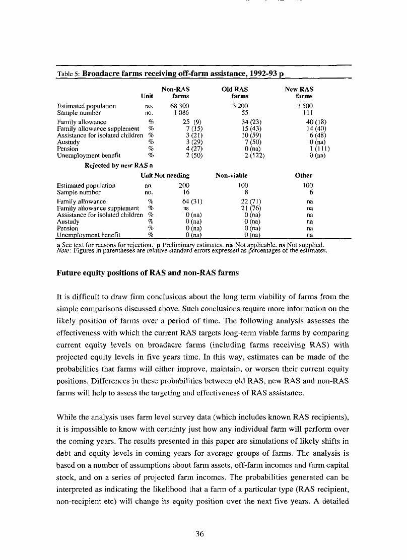
Table 5: Broadacre farms receiving off-farm assistance, 1992-93 p
Non-RAS Old RAS New RAS Unit farms farms farms
Estimated population no. 68 300 3 200 3 500 Sample number no. 1 086 55 11 1 Family allowance % 25 (9) 34 (23) 40 (1 8) Family allowance supplement % 7 (15) 15 (43) 14 (40) Assistance for isolated children % 3 (21) 10 (59)
% 6 (48)
A U S ~ U ~ Y 3 (29) 7 (50) 0 (na) Pension % 4 (27) 0 (na) l (111) Unemployment benefit 70 2 (50) 2 (122) 0 ( 4
Rejected by new RAS a Unit Not needing Non-viable Other
Estimated population no. 200 100 100 Sample number no. 16 8 6 Family allowance % 64 (3 1) 22 (71) na Family allowance supplement % 11s 21 (76) ua Assistance for isolated children % 0 (na) 0 (na) na ~us tudy % 0 ( 4 0 (na) na Pension % 0 (na) 0 (na) na Unemployment benefit % 0 (na) 0 (na) na
a See text 1;cr rmson> t i~r r~.jc-.tion. p 1'relinlin;y ~~til!i.~ld\. na Not applicrlhle. ns Not supplied. Nc~rr,: Figures in p~ren thces arc rel;~t~ve stnndar crtorb euprr.,.;r.(l as pcri~ntilfcs oi the esrlniatc?;.
Future equity positions of RAS and non-RAS farms
It is difficult to draw firm conclusions about the long term viability of farms from the
simple comparisons discussed above. Such conclusions require more information on the
likely position of farms over a period of time. The following analysis assesses the
effectiveness with which the current RAS targets long-term viable farms by comparing
current equity levels on broadacre farms (including farms receiving RAS) with
projected equity levels in five years time. In this way, estimates can be made of the
probabilities that farms will either improve, maintain, or worsen their current equity
positions. Differences in these probabilities between old RAS, new RAS and non-RAS
farms will help to assess the targeting and effectiveness of RAS assistance.
While the analysis uses farm level survey data (which includes known RAS recipients),
it is impossible to know with certainty just how any individual farm will perform over
the coming years. The results presented in this paper are simulations of likely shifts in
debt and equity levels in coming years for average groups of farms. The analysis is
based on a number of assumptions about farm assets, off-farm incomes and farm capital
stock, and on a series of projected farm incomes. The probabilities generated can be
interpreted as indicating the likelihood that a farm of a particular type (RAS recipient,
non-recipient etc) will change its equity position over the next five years. A detailed

description of the process by which future equity levels are generated is contained in
appendix A.
Tables 6, 7 and 8 contain results of the equity simulation analysis. The results indicate
some differences between farms receiving RAS before and after 1 January 1993 but it is
difficult to draw definitive conclusions from the results. A comparison of the 1992-93
equity position of new RAS farms (table 6) and old RAS farms (table 7) shows that
there were proportionately more successful old RAS recipients in the lowest equity
category compared with farms receiving new RAS. Similarly, there were
proportionately more higher equity farms receiving old RAS assistance than were
receiving new RAS. These results suggest that the new RAS may be more successful in
identifying farms with relatively low probabilities of long term viability (typically farms
which have very low equity), as well as farms which may not need assistance to remain
viable (typically farms with relatively high equity).
Table 6: New RAS recipients - equity position after five years
Equity position after five years:
Current Total Total Worse Maintain Increase farms farms
equity group no. % % of farms % of farms % of farms
< 50 per cent 370 10 78 22 50 to 75 1 864 49 18 36 46 75 to 85 992 26 4 19 77 85 to 95 553 15 9 23 68
> 95 per cent 0 0
Total 3 781 100 I 1 34 55 Note: An examole for interoretine this table: 10 Der cent of all new RAS farms had less than 50 Der - cent equity in 1992-93. Of these farms, 78 per cent are not expected to improve their equity over the next five years, while 22 per cent are expected to increase equity. Of the 1864 new RAS farms with current equity between 50 and 75 per cent, 18 per cent are expected to lose equity over the next five years, 36 per cent should maintain current equity, and 46 per cent are expected to increase equity.
By contrast to RAS farms, non-RAS farms generally have higher equity (over 50 per
cent of non-RAS farms had more than 95 per cent equity in 1992-93), but also have a
higher probability of increasing equity over time. The analysis suggest that 82 per cent
of non-RAS farms are likely to have average equity levels above 95 per cent at the end
of the next five years.
Overall, there is a similar probability of farms improving their position under both old
RAS and new RAS. However, a difference between the targeting of the old and new

RAS can be seen by comparing the performance of farms which currently have between
50 and 85 per cent equity. These farms constitute 57 per cent of old RAS recipients and
75 per cent of new RAS recipients. For these groups, farms receiving new RAS have a
higher probability of increasing thcir equity to above 95 per cent over the next five
years than farms receiving old RAS. In particular, 35 per cent of new RAS recipients in
these equity groups are likely to increase their equity to above 95 per cent over the next
five years. Only 23 per cent of old RAS recipients are likely to achieve this result (not
shown in table 6).
Table 7: Old RAS recipients - equity position after five years
Equity position after five years:
Current Total Total Worse Maintain Increase farms farms
equity group no. % % of farms % of farms % of farms
< 50 per cent 3 14 18 46 54 50 to 75 698 39 18 39 43 75 to 85 323 18 10 31 59 85 to 95 449 25 7 26 67
> 95 per cent 0 0
Total 1 785 100 10 36 54
Table 8: Non-RAS applicants - equity position after five years
Equity position after five years:
Current Total Total Worse Maintain Increase farms farms
equity group no. % % of farms % of farms % of farms
< 50 per cent 2 086 3 52 48 50 to 75 8 070 13 6 25 69 75 to 85 6 973 12 10 13 76 85 to 95 11 762 20 4 11 85
> 95 per cent 31 184 52 2 98
Total 60 076 100 4 60 36

Summary of assessment
Although the analysis and information available is preliminary at this stage, the changes
to the Rural Adjustment Scheme in January 1993 appear to have been reflected in the
better financial position of farms receiving assistance under the new scheme compared
with the old. Farms rejected for RAS tended to either be performing at least on a par
with non-RAS farms, or were classed as non-viable. The farms assessed as non-viable
tended to be characterised by extremely high interest burdens relative to their cash flow.
Although the results would tend to support the view that the new scheme achieves its
objectives, a more detailed assessment is required to verify this result.

6. Future directions for rural adjustment
Governments have a number of general objectives for the rural sector, including
attaining profitable, productive and sustainable farming across Australia. More
specifically with respect to RAS, the government has the objective of farms becoming
increasingly responsible for managing their own risk. This would enable a reduction in
the role of government in rural adjustment in the future and RAS (at least in its present
form) is scheduled to be phased out by the year 2000. The removal of some elements of
RAS assistance would mean that all farmers would be equally responsible for managing
their own risks (recognising that most farmers manage their risks without government
assistance).
Effective risk management requires that farmers have access to the necessary skills and
instruments to manage the uncertainties that they face. As mentioned earlier, there
already exists a large number of means by which farmers can manage their risks. These
include insurance markets (for normal risks), futures markets and on-farm management
measures (such as various drought strategies). There are also some income modification
mechanisms which help farmers manage their tax liabilities or smooth their incomes -
such as income equalisation deposits (IEDs), farm management bonds (FMBs) and tax
averaging. An important role for government is ensuring that the instruments it provides
to assist farmers in this regard are effective and efficient. The change to the tax
treatment of IEDs suggested earlier would assist in achieving this. Further work is
currently being undertaken on this issue.
There is not a strong argument for continuation of interest subsidies for farmers, nor for
exceptional circumstances as applied to price risks. There is a question about whether
interest subsidies are the most appropriate means of facilitating adjustment in that they
target adjustment only through borrowings. There are a range of more appropriate
instruments which directly assist the adjustment of agriculture, such as re-establishment
grants and land trading, and those which assist farmers during extreme adverse
circumstances due to natural disasters, such as parts of the exceptional circumstances
provisions. There is also a case for improved government policies with respect to the
irrigation sector, including economically efficient charging for water delivery and
increased water tradability of water rights.
Assistance for training is consistent with broader government objectives in terms of
provision of public information. Consistent with this, increased emphasis has been
placed on the training elements of RAS. As mentioned earlier, farmers may be eligible

for grants for training to upgrade farm business management skills and to assist with the
cost of obtaining financial planning and other professional advice relating to the farm
business. Between 1 January 1993 and 31 March 1994, some 2 per cent of the total
RAS expenditure and 5 per cent of expenditure excluding exceptional circumstances
was related to skills enhancement (DPIE submission). While the relative role of RAS as
compared with the normal rural education system can be considered, there is a case for
some government involvement in information provision.
Similarly, there is a case for government involvement in regional issues associated with
land degradation. In particular, efforts to encourage groups within catchments to work
together on common problems has considerable potential. Again consideration needs to
be given to the relative roles of RAS and other policies such as Landcare and
coordination between policies will be important.
Finally, it needs to be borne in mind that the need for rural adjustment arises from a
variety of sources and for a variety of reasons. In most cases, adjustment will occur in
the absence of intervention. Governments therefore need to target their efforts at
removing impediments to efficient adjustment and at the social welfare consequences of
adjustment. It is unlikely that any one instrument or policy, such as RAS, will address
all of these concerns. Rather instruments should be chosen to target specific problems
and should be placed within government to achieve maximum administrative efficiency.

Appendix A: Assumptions used in farm equity analysis
The equity analysis undertaken in chapter 5 is based on a number of important
assumptions.
First, future income variability is simulated by drawing from historical patterns of
income on survey farms in Australia over the past 15 years. The simulation incorporates
historical probabilities of good, average and poor seasonal conditions over the next five
years. The starting values for each farm (that is, beginning debt, capital, interest
payments, liquid assets, depreciation) are based on 1992-93 farm survey results.
Total income available to each farm in each of the next five years is the sum of
predicted gross cash income (derived at random from the farm-level income
distributions), total non-farm income (including off-farm wages and salaries, fixed at
1992-93 levels) and liquid assets (which may be positive or zero in any one year).
It is assumed that in each year, each farm requires $20 000 for living expenses. This
must be met from current total income before any other financial obligations are met. If
insufficient income is available, the difference is rolled over into farm debt. After
meeting living expenses, farms are required to meet interest repayments on existing
debts. If insufficient liquidity is available, the unpaid interest is rolled over into debt.
Farms are then required to meet their depreciation bill, the assumption being that real
capital levels must be maintained. Any unpaid depreciation is rolled over into debt. If
income is still positive, it is assumed that farms adjust their liquid asset holdings. Asset
levels are constrained to the maximum of average asset levels over the last five years
and 1992-93 asset levels. Finally, if income is still positive, debt principal is repaid.
This procedure is then repeated another four times until a final debt position and equity
ratio is generated.
This whole process was repeated 200 times, with each simulation providing a beginning
and ending equity position for each survey farm. The results have been tabulated to
examine the degree to which equity positions changed over the course of the five year
simulations.

Appendix B: Tax averaging, income equalisation deposits and farm management bonds
Taxation issues in agriculture cover a much wider agenda than can be presented here
and indeed there is a need for more research in this area. The focus here is limited to
risk management.
Improved farm level risk management has been identified as an important step toward
the achievement of greater 'self reliance' for farmers. Tax related instruments like
income tax averaging, Income Equalisation Deposits (IEDs) and Farm Management
Bonds (FMBs) give farmers the ability to change the expected level and variability of
their annual tax payments and therefore disposable income. In particular, because of
their effect on disposable income, tax related instruments provide a means for farmers
to manage some of the financial risks they face. Changes to these instruments could
enhance a farmer's capacity to manage such risks. Brief descriptions of current
arrangements for income tax averaging, IEDs and FMBs are provided in the box and
some details about their effects on farm income are provided in the following section.
Tax smoothing
As discussed in chapter 4, income tax averaging and IEDs allow farmers to smooth the
amount of tax they pay over time. The kind of tax smoothing offered by IEDs and tax
averaging can be justified on equity grounds. In particular, with a progressive tax
system, farmers whose income fluctuates from year to year can expect to pay more tax
than a person with the same average, but more stable, income. The extra tax burden on
those with fluctuating incomes is known as period inequity. Income tax averaging and
IEDs give farmers a mechanism for reducing the extent of period inequity.'Tax
averaging alone does not address risk management and would have to be combined with
an investment strategy. IEDs are part of an investment strategy which can limit tax
liability.
Although expected after tax income can rise with tax averaging, it also becomes more
volatile. This is because tax payments are lower when income is above average and
payments are higher when income is below average.

- - - - - - -
Box: Tax averaging, income equalisation deposits and farm management bonds
Income tax averaging If a farmer's taxable income from agricultural production is more than the average
amount calculated over the previous four years and the current year (in total, five years),
the farmer is due a rebate. If on the other hand, actual taxable income is less than the
average, the farmer is liable to pay a complementary tax. The following formula gives
the amount of tax paid under income tax averaging for a farmer with income derived
only from primary production. In this case, all taxable income is subject to averaging.
Tax in period t = (income subject to averaging at period t) x (average rate)
Average rate = (tax on average income at general rates) I (average income).
When farmers receive income not derived from primary production the amount of
income subject to averaging can differ from taxable income. For details of how to
calculate the amount of income subject to averaging in a range of different
circumstances, see CCH Australia Limited (1994).
Income Equalisation Deposits IEDs may only be used by individual primary producers (this means Lhat deposits
cannot be made in the name of partnerships or trusts). IEDs are deposited with the
Department of Primary Industries and Energy. Deposits in any one year are limited to
the amount of net taxable income from primary production in that year and total
deposits cannot exceed $300 000.
Amounts deposited into IEDs are tax deductable in the year the deposit is made. Tax is
only paid on deposits when they are withdrawn and added to taxable income. Interest is
received on an 'investment component' equal to 61 per cent of the deposit. The rate of
interest paid is equal to the short term Commonwealth Treasury bond rate. The
remaining 39 per cent is assumed to be the amount that the farmer would otherwise
have paid in tax and no interest is paid on this amount. For more details see DPIE 1994.
Farm Management Bonds In most respects, FMBs are similar to IEDs except that the investment component on
FMBs is 80 per cent, compared to 61 per cent with IEDs. Farmers with non-farm
taxable income in excess of $50 000 are not eligible to make deposits in FMBs and
deposits cannot exceed $80 000. Also deposits can only be withdrawn if the farmer can
demonstrate that a period of hardship due to natural events (including commodity price
changes) is being experienced.

Comparing ZEDS and tax averaging It is possible that tax averaging used in combination with an investment account to
smooth peaks and troughs in income could achieve similar tax and income outcomes as
an IED scheme. However, there are certain advantages and disadvantages associated
with each scheme arising from their operational aspects. An advantage of IEDs is that
they provide flexibility to farmers to smooth their incomes over any period they wish,
while tax averaging is limited to averaging income over a five year period. There is no
reason to expect that averaging over a five year period will be optimal for all farmers.
However, as discussed in chapter 4, IEDs have a number of disadvantages relating to
their tax treatment which have made them unattractive to farmers. Moreover, the
interest rate on IEDs is fixed at the short term Commonwealth Bond rate. It is possible
that farmers could get a higher return than this (albeit possibly at a higher risk) by
investing their money in other on-farm or off-farm investments. Combining tax
averaging with an investment program enables farmers to invest their money within
their preferred mix of investments while still obtaining the benefits of tax averaging. A
farmer's preferred mix of investments will depend on their preferred balance of risk and
return.
Finally, IEDs can only be used to smooth income when a farmer moves from being in a
position to initially make deposits into an IED. Hence IEDs cannot be used to assist a
farmer who has moved from a situation of a series of low income periods to a high
income period. Tax averaging, however, would enable a farmer to reduce tax payments
in the high income period as the tax paid is based on the average tax rate applying to the
average income earned in the current and preceding four years.
Possible reforms to tax averaging and IEDs Reforms to the various tax smoothing schemes could improve the range of risk and
income management options available to farmers. It is important to note, however, that
such schemes are only likely to provide substantial benefits to farmers who expect to
pay tax and who expect that their income could fluctuate between tax brackets.Tax
averaging would also become less attractive to farmers if they expected their incomes to
become less volatile, leading to a reduced risk of jumping into higher tax brackets. As
the tax structure has become flatter over recent years the benefits from tax averaging
have also declined.

In suggesting reforms to tax schemes the problem of period inequity needs to be
addressed. However, it is important to ensure that the tax system does not increase the
opportunity for farmers to manipulate farm structure in order to generate additional tax
benefits. Furthermore, it is desirable that tax arrangements be consistent across sectors
to avoid intersectoral distortions. Hence, changes to tax arrangments in the agricultural
sector should take account of tax policy as applied to other sectors.
The following few reforms to IEDs are by no means an exhaustive list of all possible
changes to the tax system affecting farmers. They are used, essentially, to highlight
some of the drawbacks of the existing system in terms of tax and risk management.
As with tax averaging the main purpose of E D s is to ensure that farmers pay tax rates
closer to their average tax rates, not at rates that would apply in years of higher than
average income. However, as noted earlier, IEDs are less likely to he attractive to
farmers who expect to face low marginal rates of tax. One way to improve the
attractiveness of IEDs to farmers as a tax and risk management tool is to make the tax
component on IEDs reflect the farmer's own marginal tax rate on average income.
There are at least two possible means for achieving this outcome.
Suggestion 1: set the proportion of the tax component equal to the marginal tax rate on
average income
This is administratively more difficult than the current flat investment component
structure as tax components would need to be set individually. Also, after periods of
high income, when farmers are most likely to accumulate IEDs, average income as
calculated for averaging is above true average income. As a result the tax component of
LEDs may be systematically too high.
Suggestion 2: have a 100 per cent investment component and increase the tax paid on
interest
Under this suggestion the investment component is raised to 100 per cent but a higher
rate of tax is payable on the interest earned from IEDs. The higher rate chosen is
equivalent to having an investment component set with reference to the farmer's current
marginal tax rate.
The rate of tax suggested is 2r- r2 where r is the farmer's current marginal tax rate. An
explanation for this choice of rate is contained below. This system has the advantage
that the farmer's own tax rate determines the appropriate investment component. As the

tax component needs to be set on an individual basis each year, this suggestion is more
administratively complicated than the current system.
Taring the interest from ZEDS
It was suggested above that the investment component of IEDs could be removed and
tax on interest could be payable at a rate of 2r - r2 . This can be demonstrated as
follows.
Consider a person who saves $1 of pre-tax income for ever drawing only on the interest.
The person does not get to save $1. Instead they would normally save $(I-r) where r is
the marginal tax rate. The interest received each year would be $i(l-r) where i is the
interest rate. Tax is then paid each year on the interest at a rate i so the person
eventually receives $i(l-r)2.
This is conceptually the same as the person paying tax at the rate of 1-(1-r)2 on the
original income or paying no tax until the interest is drawn and paying 1-(1-r)2 = 2r-
r2 on the interest.
Under IEDs, if the person were to be pcrmittcd to save pre-tax income with interest paid
on the whole investment then the effective tax rate would be r. Comparing this with the
above estimate of tax paid by a person undertaking normal savings ( 2 r - r2) a sizeable
concession is being made. For example, if r were 0.3 (30 per cent), this gives an
effective tax rate of 0.3 for the concessional IED versus 0.51 for normal savings. This
provides the basis for the current IED investment component and the suggested
additional taxation of interest on IEDs (at a rate of 2 r - r2).

References
ABARE 1993, Commodity Statistical Bulletin 1993, Canberra.
- 1994, Farm Surveys Report 1994, Canberra.
CCH Australia Limited 1994, Australian Income Tax Guide, volume 2, Sydney.
Cloney, J . 1994, 'Farm and crop insurance', in QBE Insurance, Manage Your Risk,
Control Your Future, Cox Inall Communications, pp. 20-22.
CSIRO Institute of Natural Resources and Environment 1990, Australia's Environment
and its Natural Resources, Canberra.
Department of Primary Industries and Energy 1994, Income Equalisation Deposits,
Canberra.
Findlay, C.C. and Jones, R.L. 1982, 'The marginal cost of Australian income taxation',
Economic Record, vol. 58, no. 162, pp. 253-62.
Hall, N., Poulter, D. and Curtotti, R. 1994, ABARE Model of Irrigation Farming in the
Southern Murray-Darling Basin, ABARE Research Report 94.4, AGPS,
Canberra.
Industries Assistance Commission 1984, Rural Adjustment, Assistance Report no. 344,
15 March, Canberra.
Leathers, H.D. and Chavas, J.P. 1986, 'Farm debt, default and foreclosure: An economic
rationale for policy action', American Journal of Agricultural Economics,
November, pp. 828-837.
Males, W.P., Davidson, H., Knopke, P., Loncar, T., and Roarty, M.J. 1990, Productivity
Growth and Developments in Austrulia's Primary Industries, ABARE Discussion
Paper 90.8, AGPS, Canberra.
Morris, P., Wilks, L. and Wonder, B. 1992, in Wallace, N. (ed.), 'Natural resource
management: some economic and policy considerations', Natural Resource
Management: an Economic Perspective, chapter 1, AGPS, Canberra, pp. 3-27.

Mues, C., Roper, H. and Ockerby, J. 1994, Survey of Landcare and Land Management
Practices: 1992-93, ABARE Research Report 94.6, AGPS, Canberra.
Musgrave, R.A. 1985, 'A brief history of fiscal doctine', in Auerbach, A.J. and
Feldstein, M. (eds), Handbook of Public Economics, volume 1, chapter 1, Elsevier
Science Publishers B.V., Amsterdam, pp. 1-59.
OECD 1993, Agricultural Policies, Markets and Trade, Monitoring and Outlook, 1993,
Paris.
Prime Minister 1994, Working Nation, White Paper on Emplo.yment and Growth, 4
May, AGPS, Canberra.