1

IX/ADRT/112

RURAL NON-FARM EMPLOYMENT IN KARNATAKA

D.V. Gopalappa

Agricultural Development and Rural Transformation Unit Institute for Social and Economic Change

Nagarabhavi, Bangalore 560-072

February 2004

2

CONTENTS

Chapter No. Chapter – 1 Chapter – 2 Chapter – 3 Chapter – 4 Chapter – 5 Chapter – 6 Chapter – 7

Preface Acknowledgements Introduction A Brief Account of the Pattern of Rural Non-Farm Employment in Karnataka State Non-Farm Employment in the Sample Districts – Secondary Data Analysis Village Level Rural Non-Farm Diversification Household Level Rural Non-Farm Diversification Status of Enterprises in the State with Special Reference to the Processing Sector Livestock Based Processing Sector in the State References

3

PREFACE

The wave of the changing context of markets and gradual withdrawal of the state

from its interventionist role will place the agricultural sector at difficult crossroads. Five

decades of experience of Indian agriculture has clearly shown that the share of Net National

Domestic Product emerging from agricultural sector, has been sliding down at a faster rate,

but at the same time the share of workforce dependent on agriculture is not declining with a

similar rate. This has caused increase in the carrying capacity of the sector. Overall it

indicates the failure of Lewisian framework of transfer of labour from agriculture to non-

agricultural sector and an impending reduction in the quality of life in the agricultural sector.

In addition to this the growth rates in employment in agriculture as well as non-agricultural

sectors are also not quite encouraging. As a result, the pressure on employment in the non-

farm sector is increasing significantly. The demand for Non-Farm Employment (NFE) is

largely confined to skilled workers and therefore, the growth in employment is moving at

snail’s pace. Keeping in view the importance of non-farm sector in the calculus of quality of

life, it was felt necessary to carry out a holistic and widespread study on NFE. The Ministry

of Agriculture GoI initiated a project to analyse the trends and determinants of NFE in

various states. This study was focused to analyse the pattern and diversification of the

emerging non-farm sectors in various states in the country. The growth and the determinants

of the non-farm sector naturally became important components of this study.

Dr. D.V.Gopalappa undertook the study at ADRT unit at a very short notice. But he

completed it quite competently. Dr Brajesh Jha, Institute of Economic Growth, New Delhi,

provided the study design as well as the methodology and questionnaire. The study was

carried out both at secondary as well as primary data level and the results indicate good

prospects for non-farm sectors in the districts of Karnataka provided such efforts are

supported by the State or the non-state institutions. It is pointed out that increase in the NFE

will be influencing the quality of life of the population significantly. I am sure that the results

of the study will be of great use to the policy makers and academicians.

R S Deshpande Professor and Head

ADRT Unit, ISEC, Bangalore.

4

ACKNOWLEDGEMENTS

This study began at the initiation of the Ministry of Agriculture, coordinated by the Institute of Economic Growth, New Delhi. The study is being conducted in all the Agro-Economic Research Centres of the country. I thank Professor V.M.Rao for his good words and encouragement from time to time to carry out the study. I thank Dr. Brajesh Jha, the coordinator of the project, IEG, who was kind enough to clear doubts about the project. At the Institute, Prof. Gopal K Kadekodi, Director, Institute for Social and Economic Change, has been helpful and encouraging me to carry out the work. Dr. R.S.Deshpande, Professor and Head ADRT unit, has also given me encouragement to complete the project and also provided me with two excellent investigators to complete the field work. Dr. M.J. Bhende, a senior colleague of mine, has been helpful in advising and clarifying the doubts regarding the project. I thank all of them for their kind help and encouragement.

The respondents of Dakshina Kannada and Raichur districts deserve a special mention for withstanding our long schedule of questions and the strenuous process of enquiry. This study is entirely indebted to their wholehearted support and I would be very happy if the study helps them in terms of policy formulation to augment their welfare. I sincerely thank the officials of the Department of Industry of the respective districts who helped me in so many ways to complete the data collection. Shri H.S. Gangadhar and Shri Rajendra B Desai were the two research assistants in this project, deserve a special thanks. They were involved in data collection and tabulation. I therefore, acknowledge their effort and thank them. I thank Shri Mohan Kumar for his help in desktop publishing and taking the final print of the report. I thank Shri Devraj for his help in Xeroxing the material required for the project. The errors of interpretation and commission are entirely mine and I shall be responsible for them.

Dr. D.V.Gopalappa Asst. Professor

ADRT Unit Institute for Social and Economic Change

Nagarabhavi Bangalore 560 072

5

CHAPTER I

INTRODUCTION Introduction Even after 56 years of independence, the majority of the population of our country

lives in villages and depend on agriculture for their livelihood. However the share of

agriculture in the National income has been declining and is estimated to come down to less

than 25 per cent. This has aggravated the unemployment and underemployment situation in

rural India. The other major source of employment, industry, had not made any

breakthrough in the rural areas. On the other hand, projections based on the growth rate of

labour force at 2.5 per cent per annum indicate the necessity of providing additional

employment for about 94 million people. The agricultural sector, due to declining size of

holding and the organized industry have not been able to generate the needed employment

opportunities. This underscores the need for alternative avenues for employment generation

in the rural areas. This brings the development of the Non-Farm Sector (NFS) into focus

(Rajasekhar 1995).

`Non-Farm’ sector means all the non-crop agricultural activities; it includes

manufacturing activities, mining and quarrying, transport, trade and services in rural areas.

And also the seasonal and contractual jobs unconnected with farming as such, available

within the village or a nearby town are considered part of NFE. Rural Non-Farm Activities

(RNFAs) play an important role in developing countries such as India. These activities

provide supplementary employment to small and marginal farm households especially during

the slack season. Consequently, incomes of these households tend to be smooth in a year.

RNFAs also have potential to reduce income inequalities and rural-urban migration

(Rajasekhar, 1991; 12-15). The non-farm sector is, therefore, seen as a method by which the

problems of unemployment, particularly rural unemployment, can be tackled and poverty can

be reduced and many efforts are being made in this area of work.

There is abundant literature on the rural non-farm sector. Several studies

(Vaidyanathan, 1986; Unni, 1991; Basu and Kashyap 1992; and Dev 1990 and 2003),

drawing data from NSS and Census reports, have looked at the growth and structure of NFE

6

across various regions and factors determining the variations in NFE. There are not many

studies which analyse the types, characteristics and factors contributing to the growth of

NFAs at the village level. Though the literature is growing, there are gaps. First, the studies

on factors contributing to NFE treat the non-farm sector as homogenous. Hence, it is

imperative to analyse the factors contributing to the emergence of different activities at the

micro level. Second, the studies analysing the factors contributing to NFE are at the macro

level. There is a need to analyse the growth, structure and factors contributing to the NFAs

at the micro level. Third, it is argued that the new economic policies introduced since 1991

have had an adverse impact on the unorganised non-agricultural sector in rural and urban

areas. In this context, it is important to verify these arguments at the micro level.

The changing composition of the rural labour force at the macro level since 1961 has

been characterized by three major features. One, the share of non-farm activities in the total

labour force has been increasing, albeit slowly; two, this increase has come mainly from the

tertiary sector; and three, the bulk of the increase in NFE has been casual in nature (Visaria

and Basant, 1994, p.18). The increase in the non-farm component of the rural workforce has

been attributed to both developmental and distress factors which sometimes have been

operating in a mutually reinforcing way (Vaidyanathan, 1986). The developmental factors

like agricultural modernization and commercialization, increased demand for non-crop goods

and services, urbanization, growing literacy and even welfare-oriented policy interventions

leading to increased job opportunities, etc., have tried to pull the labour force away from

agriculture towards more lucrative non-farm activities. At the same time, distress factors like

poverty, unemployment/underemployment due to the inability of agriculture to absorb

surplus labour, and even frequent natural calamities like drought have tried to push rural

households to search for various NFAs activities to supplement their farm income and

employment. However, wide regional variations in the nature and composition of this labour

force, combined with serious data limitations, have prevented the studies attempting to

capture the said process from arriving at any definite conclusion. Hence an increased

emphasis has now been laid on the need for conducting more focussed micro/village level

studies, which can capture the process, factors and the determinants of the ongoing

occupational diversification.

There have been studies to assess the determinants of RNFE (RNFE) (Acharya and

Mitra 2000; Basant et.al. 1998); but most researchers have tried to substantiate one of the

7

above propositions about the process of NFE diversification. Their approaches were

different, so were the results. Often aggregation of data has also contributed to this

confusion; data on the NFS aggregated even at the micro level may not show clear cut trends;

since a wide range of activities are being pooled together. Therefore, a disaggregated

analysis of the factors responsible for the diversification of RNFE at the Household (HH) is

desirable. The present study will be focussed on the aforementioned.

In order to address some of these concerns the present study focussed on the

following objectives;

1. To study the pattern of RNFE diversification, at the HH level.

2. To estimate the determinants of employment in selected non-farm rural activities.

3. To assess region-specific constraints in the growth of livestock–based agro-processing

units.

Methodology:

As part of a study coordinated by the Agro-Economic Research Center, Institute of

Economic Growth, New Delhi, ADRT unit has conducted present study in Karnataka State.

To fulfill the first and second objectives of the study about employment diversification at the

household level and to select the sample households multi-stage stratified random sampling

techniques we adopted. Two districts were selected for the study, one district having the

highest density of non-farm workers and another district having the lowest density of

workers. The available secondary data shows that Kodagu, Dakshina Kannada (DK) and

Chickmagalur districts have the highest concentration of non-farm workers and ranks first in

all the three years under study (1971, 1981 and 1991). Therefore, we have selected DK by

lottery method out of these three districts. Three districts were considered for the lowest

concentration viz., Raichur, Mandya and Shimoga districts. The latest figures of 1991

showed Raichur in the 19th position compared to Mandya and Shimoga districts, which were

in the 16th and 18th places respectively. We put all the three districts in the selection list and

Raichur district was selected based on the same lottery method.

8

In the second stage of sampling, two village clusters (each consisting of three

villages) from each of the selected districts were selected on the basis of level of employment

diversification in the villages. Available literature indicates proximity to town as the most

important determinant of NFE diversification in a specific region; therefore two villages

clusters, one cluster situated within 3 kms of a town and another cluster situated more than

10 km away from any town were selected in each district.

A sample of 30 rural households was selected randomly from each of the village

clusters. The proportion of these categories of households in the sample was based on their

distribution in the village population; however, a minimum of 3 households in each category

were selected based on the random sampling method. In brief, 2 districts were selected on

the basis of concentration of non-farm rural workers, 2 village clusters from each of the

selected districts were chosen on the basis of proximity to a Class II town, and 30 sample

HHs were studied from each village cluster - altogether 120 households, 4 village clusters,

and 2 districts from each state.

To fulfil the third objective, the coordination centre had suggested four livestock-

based activities i.e., milk, wool and meat to find out the prospects of employment generation.

Hence we selected fishing activity as it was one of the livestock-based activities in DK

district. Two villages (Kotepura and Mukka) in Mangalore taluk where the fish-processing

activity is very significant, were selected for this purpose. In Raichur district we found that

leatherwork was the major livestock activity. Therefore, two villages (Maski and Gurgunta)

in Lingsoor taluk of the same district were taken for the study (selection of the households

and manufacturing units were done as per the guidelines given in the proposal).

Meaning and Importance of the Non-Farm Sector:

The term `non-farm’ encompasses all non-crop agricultural activities; it includes

manufacturing activities (cottage and small rural industries and other forms of petty

production), trades and services in rural areas. And also, the seasonal and contractual jobs,

unconnected with farming as such, available within the village or in the nearby town, are a

part of NFE (Chadha, 1986; 141: Edgreen and Mugtada, 1989; 38). RNFAs constitute an

important category of income for the poor in developing countries which are characterised by

problems such as mounting population pressure, diminishing land frontiers, small and

fragmented landholdings due to declining land-man ratio and a high incidence of

9

unemployment. The non-farm activities provide supplementary employment to small and

marginal rural households, especially during the slack season. Thus, in determining the total

employment and income status of small and marginal households, non-farm activities have a

place of great significance in a rural society.

Importance of Non-Farm Sector:

In recent years, there has been a growing realisation among academics and policy

makers in India that the nature of the links between different sectors need to be re-examined.

As discussed above, the earlier belief that the secondary sector would productively absorb

labour released from the primary sector may not be the only pattern of growth possible – or

even desirable. It may be essential to adopt the production methods of the secondary sector

such as division of labour, new forms of organisation of the work-processes and so on, in

rural areas so that the growth process does not necessarily require an increasing urban

industrial sector. The focus shifts from spatial rural/urban dichotomies to the nature of

linkages between economic activities and processes. It is the strengthening of such links that

is sought to be conveyed in what is now being called the non-farm sector in the literature

(Vyasulu, 1990). RNFAs, once developed, would lead to the following beneficial effects on

rural communities.

Income from Non-Farm Activities:

Lack of primary data on wages and income from RNFAs in India makes it difficult to

establish the structure and importance of non-farm earnings for rural household incomes.

Liedholm and Kilby (1989) found that non-farm activities are second in importance to

agriculture in several countries of the world in terms of their contribution to GNP. Evidence

from five countries in Asia and Africa suggests an inverse relationship between the size of

landholding and the share of non-farm income in the total household income. For the

smallest landholding categories in each country, non-farm income sources accounted for

more than 50 per cent of household income (Liedholm and Kilby, 1989; 346). Thus, NFAs

are important for enhancing the income of small and marginal rural HHs (Samuel 1979).

There is also evidence to show that non-farm activities reduce income inequalities in

rural areas (Samuel 1979). Non-farm sources cause the total incomes of the rural households

with small landholdings to exceed the incomes of those with large landholding sizes. This

vertical relationship between the rural household income and landholding seems to be

10

holding true only in some parts of the world. One problem with this methodology is that the

farm size is taken as a proxy of the total rural household income; but rural household income

levels are determined by factors such as farming, non-farm enterprises, off-farm trading and

employment opportunities. Hence, it would be better to take the share of non-farm income in

total household income. The information on this is scarce. However, such data, wherever

available, revealed that `vertical’ shaped relationship holds true. Thus, rural non-farm

income is relatively important at both ends of the income distribution.

The RNFAs also reduce rural-urban migration. The decentralised industrialisation in

Taiwan, for instance, has created rural employment opportunities and enabled a large number

of Taiwan’s population to participate in industry without having to leave the countryside.

This has not only reduced the total need for urban housing and infrastructure but also made

the transition from agricultural to non-agricultural activity less abrupt, with fewer disruptions

of family life and the rural social fabric (Samuel 1979). Clearly, there is much to learn from

the experience of countries like Taiwan.

Size and Trends in Non-Agricultural Employment:

The percentage of non-agricultural workers in rural areas seems to be increasing in

most of the developing countries. Anderson and Leisonson assessed the extent and

importance of non-farm activities in rural areas and towns from the viewpoint of their

contribution to the output employment and earnings of the rural workforce. It is rather

difficult to arrive at the levels of RNFE because of differences in concepts employed in the

National Census and nation wide labour surveys. Anderson and Leisonson, by making

adjustments in the National Census data across 15 developing countries, conclude that non-

farm activities in rural areas are a primary source of employment and earnings for

approximately one quarter of the rural labour force in most of these countries (one-third

including the labour force in the rural towns), and a significant source of secondary earnings

in the slack seasons for the small and landless farmers. In African countries, rural non-farm

activities account for over two-thirds of all NFE (both urban and rural), in Asia for over one-

half, and in Latin America for over one-third (including activities in rural towns) (Anderson

and Leisonson, 1980; 228-29: Liedholm and Kilby, 1989; 341-345).

For the estimates of the size of rural non-agricultural employment in India, we have

two sources, namely population censuses and National Sample Surveys (NSS). From the

11

population Censuses, one can get some idea of the proportion of the rural population engaged

in economic activity and their distribution by sector of employment. However, a detailed

sectoral breakup of the working population is available only up to the state level and this

limits the usefulness of these data. And also “problems of determining the activity status of a

particular individual, the fact that workers often do several types of work covering different

`sectors’, and the difficulties of capturing the intensity of employment in a short

questionnaire administered at a single point of time’ have severely limited the utility of the

census data (Vaidyanathan, 1986; A-130).

Factors Determining Regional Variations in Non-Agricultural Employment:

There is a moderate shift of workers from agricultural to non-agricultural activities

and such a shift has inter-regional, gender and function-wise variations. What does this shift

of workforce from agriculture to non-farm sector imply? This shift can be attributed to a

rapid increase in non-agricultural employment opportunities as a consequence of economic

development, pulling semi-employed and under-employed workers from agriculture. This

can also be attributed to commercialised agriculture which is pushing out semi-employed and

under-employed workers, so that non-agricultural sector is now turning into the location for

rural surplus labour. While the first proposition implies productive RNFE, the latter points

towards `distress diversification’. It is in this context that an understanding of factors

contributing to RNFE becomes pertinent. The studies by Vaidyanathan, Mahendra Dev and

Jeemol Unni, among others, seek to analyse the factors determining RNFE in India. The

factors, which were elaborated in these studies, can be summarised below.

Linkages Between Agricultural Development and Rural Non-Farm Activities:

Rural non-agricultural employment naturally depends on agricultural prosperity in a

region. Because the incomes of a great majority of people in India depend on the

performance of the agricultural sector, the demand for consumer and other types of goods by

them depend on agricultural prosperity. The same was noted by Raj (1976), `Conditions are

favourable for the more extensive and rapid growth of small-scale industries in only some

regions in India i.e., those which have recorded moderate to high rates of growth of

agricultural output without being subject to serious fluctuations’. This hypothesis is sought

to be tested across several countries. For instance, Anderson and Leisonson (1980) found

that non-food goods and services occupy a rising share of the rural households’ budget as

income rises. In the case of India, Papola (1987) found that the performance of rural

12

industrial sector in different states broadly corresponded with levels of agricultural

productivity and more closely with the growth rate of agricultural output. Rise in income

levels, purchasing power and to an extent the investible surplus generated by agricultural

growth improved the efficiency of the existing industries and led to the emergence of new

and dynamic areas.

Vaidyanathan (1986) considered the level of rural employment in rural non-

agricultural activity to be a function of (1) the level of rural demand for non-agricultural

goods and services produced locally; (2) the level of extra demand for rural products

(services); and (3) the location, scale and technology of activities catering to these demands.

He used crop output per head of agriculture population to test the hypothesis of agriculture-

led NFE. He found that crop output per head of agricultural population had a significant

positive impact on the incidence of non-agricultural activity. Dev’s (1990) analysis at the

level of NSS regions showed that output per hectare (land productivity) seems to have a

positive impact on non-agricultural employment. Unni (1991) found mixed evidence to this

hypothesis. She notes; ‘the hypothesis of agriculture led growth is partly substantiated by a

positive relationship between agricultural productivity in a region and percentage of non-

agricultural employment. At the dis-aggregated level, this appears to positively influence

non-agricultural employment in all industry groups, except electricity, gas and water and in

both developed and less developed regions. Rapid growth of agricultural production in the

previous decade, however, appeared to absorb labour better in the agricultural sector.

Production Linkages:

The growth of rural non-agricultural activities also depends on backward and forward

linkages that the rural non-agricultural sector has with agriculture. For instance, the

manufacture and repair of agricultural implements and transport, act as horizontal linkages

from the non-agricultural sector to agriculture. Likewise, processing of products from

agriculture (such as cotton, tobacco, groundnuts, sugarcane, etc.,) are forward linkages from

to agriculture. Supply of manufactured inputs, characteristic of modern technology, eg.,

fertiliser, pesticides etc., are a backward linkage. Papola (1987) found that by supplying raw

materials (backward linkages) and creating demand for input and allied services (forward

linkages) there will be a rapid agricultural growth and this has direct impact on RNFAs. The

indirect impact was through raising consumption demand and generating surplus for

investment. He found more evidence for an indirect relationship rather than a direct one.

13

The degree of commercialisation is taken as a proxy for forward and backward

production linkages. Vaidyanathan hypothesised that commercialisation of agriculture would

lead to higher RNFE. Vaidyanathan used three variables as a proxy of degree of

commercialisation. (1) the level of crop output per head of agricultural population (2) the

distribution of land ownership and (3) the proportion of area under non-food crops. The

percentage area under non-food crops gave mixed results in the regression analysis and

Vaidyanathan advocated further refinement in the variable on commercialisation before

coming to any conclusion. In Unni’s (1991) analysis, the cropping pattern did not indicate

any positive impact when analysis was done at all regions. In fact, it was negatively and

significantly related to the percentage of female non-agricultural workers. Thus,

commercialisation of agriculture in a region appears to inhibit rather than facilitate female

participation in rural non-farm activities. However, at a disaggregated level, the dominance

of non-food crops had a direct positive impact on male employment in transport, storage and

communications.

Level of Urbanisation:

The proximity to or existence of a large urban population in a region may also

facilitate the growth of non-agricultural employment in rural areas in the following ways.

The rural areas may cater to the demand for non-agricultural products and services in the

nearby urban areas. Secondly, some of the residents from rural areas may engage in non-

agricultural occupations in the nearby town and commute to their work place regularly.

Jeemol Unni found that, at the aggregate level, the percentage of urban population had a

positive impact only on male non-agricultural workers. At a dis-aggregated level,

urbanisation had a positive impact in most of the industry groups except in construction and

personal services as the demand for these activities is generated in the rural areas itself and

they also do not require support from infra-structural facilities available in urban areas (Unni,

1991).

NFE as a Residual Sector:

The second dimension to the growth of rural non-farm activities can be termed as

‘distress diversification’ into unproductive or low paid non-agricultural jobs. Such a distress

diversification occurs especially when the workers are under-employed in agriculture and the

non-agricultural sector acts as a sponge for the excess labour. Such a spill off of excess

14

labour from agriculture to the rural non-farm sector has been put forward as the residual

sector hypothesis by Vaidyanathan (1986). He used NSS person day unemployment rate to

capture the excess labour problem in agriculture leading to the growth of residual non-

agricultural activities. He found a strong positive relation between the unemployment rate

and the percentage of non-agricultural workers. Unni (1991) treated this problem much more

elaborately. She questioned the validity of taking NSS person day unemployment rate for the

following reasons. First, NSS unemployment rate captures only visible and open

unemployment, which would be higher in agriculturally developed regions as the people

flock to these areas with expectations of better employment. Added to that, such reported

unemployment would be higher in wage dependent households or casual labourers than in

self-employed households because it is easier for casual workers to perceive and report their

unemployment. The proportion of casual labourers would be high in agriculturally

developed regions. If that is the case, the percentage of non-agricultural workers will be

higher in these regions. It is not surprising that a positive relationship between these two was

observed. In fact, she found a strong positive correlation between the unemployment rate

and the index of agricultural development and agricultural productivity per hectare, as well as

between the latter two and the percentage of non-farm workers in 56 NSS regions.

Second, the residual sector hypothesis implies that the high unemployment rates

should depress the non-agricultural wage relative to the wage in agriculture. An analysis of

the correlation between the percentage of non-agricultural workers and the wages in the non-

farm sector relative to those in the farm sector in 56 NSS regions showed the association

between these two variables. Thus, the hypothesis that surplus labour from agriculture is

pushed out to the non-farm sector is not substantiated at the dis-aggregate level.

The weak empirical support to the `distress diversification hypothesis’ at the dis-

aggregate level, is thus due to incorrectness of using NSS person days unemployment rate.

Hence, Jeemol Unni takes two variables, namely the percentage of landless rural labour

households and the percentage of the population below the poverty line. She found mixed

evidence when these two variables were incorporated into the regression model. She

concludes: “in regions with a higher proportion of poor population, the percentage of male

workers in non-agriculture was low. This would imply that distress conditions do not

necessarily lead to the growth of non-agricultural activity, perhaps due to lack of demand for

non-agricultural goods in such regions. However, it was also observed that above a certain

15

level regions with a high proportion of landless labour households had a higher percentage of

male non-agricultural workers. Here at least exists the possibility of an excess labour supply

from these households leading to non-agricultural activity. When the regions were dis-

aggregated by level of development, this relationship was observed in the developed regions

but not in the less developed regions” (Unni 1991). Thus, the debate on whether the growth

of NFE is ‘distress diversification’ or not remains inconclusive (Unni, 1998). One reason for

this is that so far, the studies on this question have concentrated mainly on macro evidence.

We need to have primary studies of rural households, where the decision making regarding

the allocation of labour is done.

16

CHAPTER II

A BRIEF ACCOUNT OF THE PATTERN OF RURAL NON-FARM

EMPLOYMENT IN KARNATAKA STATE

In this chapter an effort is made to understand the percentage share of agriculture and

non-agriculture in total workers, the percentage of agricultural workers by industry category

and sex in rural Karnataka, and to make a region-wise analysis of RNFE in the state.

Towards this the census data of 1961 to 2001 and also the NSSO data of 27th to 55th rounds

have been used. However, wherever data is not available that has been excluded from the

analysis.

Table-2.1 presents the percentage of agricultural and non-agricultural workers to total

workers in Karnataka state for the five census periods. The proportion of total agricultural

workers was about 70.55 per cent in 1961, which has started declining continuously over the

decades. By 2001 the percentage was 55.89 per cent. The same trend can be noticed even in

the case of male and female agricultural workers. However, the percentage of female

agricultural workers has been high when compared to the male agricultural workers though

the rate has come down over a period of about 40 years. In case of non-agricultural labour

the percentage has been going up over a period of time. As on 2001 the percentage of male

agricultural workers is high, 50.86 per cent when compared to the agricultural labourers

constituting only 49.14 per cent. The female non-agricultural workers is much low (31.63

per cent) when compared to the agricultural labourers constituting 68.37 per cent. The same

results relating to gender are brought out by Chadha (2001) and Dev (1990) at the all-India

level. This may be due to the free mobility of male labour from one place to another.

Female labourers’ mobility is lower because of a few factors. First (as reported by our

respondents in the study areas), women have to attend to household work; second, they have

to take care of the children; third, they have lower levels of education and finally they have

security concern. All these are major factors affecting their lack of mobility (Chadha 2001).

Therefore, they try to stick to agriculture operations and agricultural labour.

17

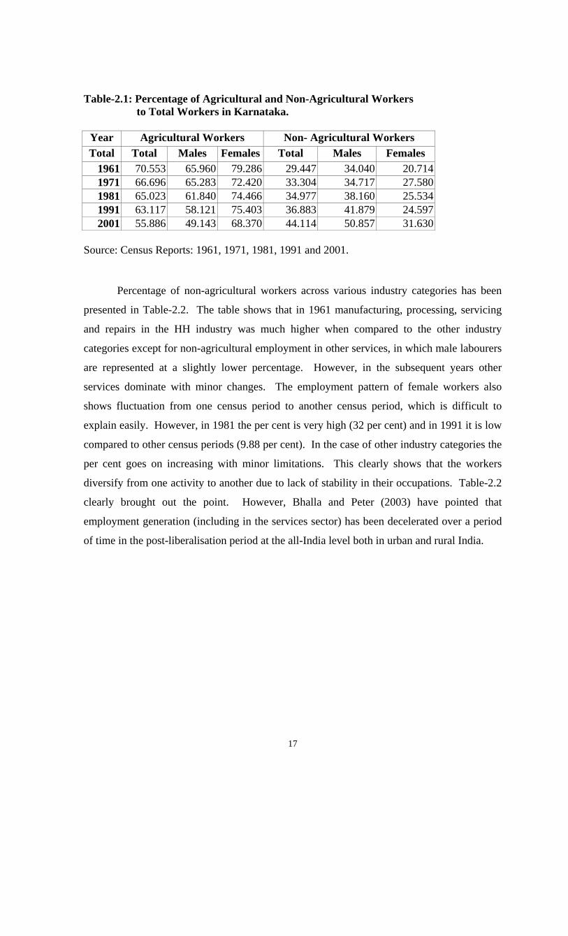
Table-2.1: Percentage of Agricultural and Non-Agricultural Workers to Total Workers in Karnataka.

Year Agricultural Workers Non- Agricultural Workers Total Total Males Females Total Males Females

1961 70.553 65.960 79.286 29.447 34.040 20.714 1971 66.696 65.283 72.420 33.304 34.717 27.580 1981 65.023 61.840 74.466 34.977 38.160 25.534 1991 63.117 58.121 75.403 36.883 41.879 24.597 2001 55.886 49.143 68.370 44.114 50.857 31.630

Source: Census Reports: 1961, 1971, 1981, 1991 and 2001. Percentage of non-agricultural workers across various industry categories has been

presented in Table-2.2. The table shows that in 1961 manufacturing, processing, servicing

and repairs in the HH industry was much higher when compared to the other industry

categories except for non-agricultural employment in other services, in which male labourers

are represented at a slightly lower percentage. However, in the subsequent years other

services dominate with minor changes. The employment pattern of female workers also

shows fluctuation from one census period to another census period, which is difficult to

explain easily. However, in 1981 the per cent is very high (32 per cent) and in 1991 it is low

compared to other census periods (9.88 per cent). In the case of other industry categories the

per cent goes on increasing with minor limitations. This clearly shows that the workers

diversify from one activity to another due to lack of stability in their occupations. Table-2.2

clearly brought out the point. However, Bhalla and Peter (2003) have pointed that

employment generation (including in the services sector) has been decelerated over a period

of time in the post-liberalisation period at the all-India level both in urban and rural India.

18

Table-2.2: Percentage of Workers in Various Industry Sectors in Rural Karnataka (Decadal Results

Industry Categories

1961 1971 1981 1991 2001

Total Males Females Total Males Females Total Males Females Total Males Females Total Males FemalesIII. A.Act. 17.01 17.02 17.00 23.19 22.54 25.76 22.49 22.01 24.05 20.61 20.04 22.47 5.22 3.61 8.48

IV. M & Q. 0.00 0.00 0.00 2.00 1.94 2.25 2.08 1.99 2.38 3.07 3.10 2.97 94.78 96.39 91.52

Va.HHI 30.98 28.72 36.35 18.13 15.92 26.82 17.79 13.46 32.02 7.97 7.37 9.88 0.00 0.00 0.00

Vb.NHHI 6.42 7.27 4.43 10.63 11.21 8.35 16.75 16.70 16.90 19.57 15.07 34.05 0.00 0.00 0.00

VI. Contn. 5.20 5.90 3.53 5.81 6.15 4.47 5.69 6.38 3.41 5.47 6.62 1.78 0.00 0.00 0.00

VII. T&C. 9.21 9.79 7.82 12.46 13.54 8.21 13.79 15.30 8.82 16.57 18.62 9.97 0.00 0.00 0.00

VIII. TS&C. 1.43 2.00 0.07 3.27 3.76 1.34 4.38 5.39 1.07 4.67 5.99 0.42 0.00 0.00 0.00

IX. Otrs. 29.75 29.31 30.80 24.51 24.94 22.81 17.03 18.76 11.36 22.07 23.19 18.45 0.00 0.00 0.00

Total 100 100 100 100 100 100 100 100 100 100 100 100 100 100 100

Note: 1). In case of 2001, we have just two industry categories i) Household industry category and ii) Other categories. 2). The industry categories can be read as i). III. Aact = Livestock, Forestry, Fishing, Hunting and Plantations, Orchards and Allied Activities. ii). IV. M&Q = Mining and Quarrying iii). Va. HHI = Manufacturing, Processing, Servicing and Repairs in Household Industry. iv). Vb. NHHI = Manufacturing, Processing, Servicing and Repairs in Non- Household Industry. v). VI Contn = Constructions vi). VII T&C = Trade and Commerce vii). VIII TS&C = Transport, Storage and Communications viii). IX Otrs = Other Services. Source: As in table 2.1. Using NSSO reports, data has been collected for agricultural employment and non-

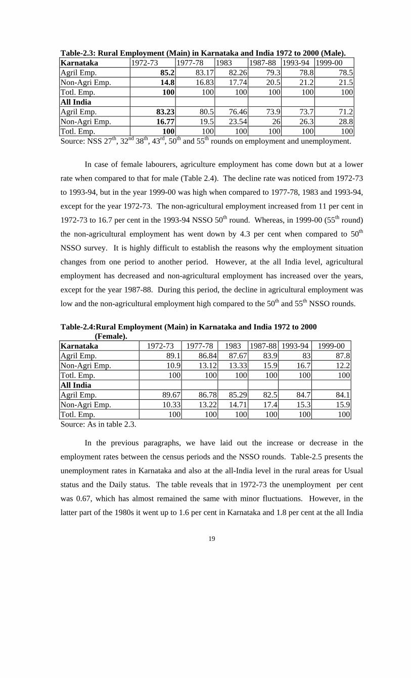
agricultural unemployment for both Karnataka and at the all India level. Table-2.3 presents

male employment in both agriculture and non-agriculture employment. As was the case with

census data, here also we found that between the various NSSO rounds, agricultural

employment for males kept on declining and the non-agricultural employment went on

increasing. The per cent of the former was 85.2 per cent in 1972-73, which had declined to

78.5 per cent by 1999-00. The non-agricultural employment was 14.8 per cent in the same

year, which increased to 21.5 per cent. Even at the all-India level also we found the same

trend.

19

Table-2.3: Rural Employment (Main) in Karnataka and India 1972 to 2000 (Male). Karnataka 1972-73 1977-78 1983 1987-88 1993-94 1999-00 Agril Emp. 85.2 83.17 82.26 79.3 78.8 78.5Non-Agri Emp. 14.8 16.83 17.74 20.5 21.2 21.5Totl. Emp. 100 100 100 100 100 100All India Agril Emp. 83.23 80.5 76.46 73.9 73.7 71.2Non-Agri Emp. 16.77 19.5 23.54 26 26.3 28.8Totl. Emp. 100 100 100 100 100 100Source: NSS 27th, 32nd 38th, 43rd, 50th and 55th rounds on employment and unemployment.

In case of female labourers, agriculture employment has come down but at a lower

rate when compared to that for male (Table 2.4). The decline rate was noticed from 1972-73

to 1993-94, but in the year 1999-00 was high when compared to 1977-78, 1983 and 1993-94,

except for the year 1972-73. The non-agricultural employment increased from 11 per cent in

1972-73 to 16.7 per cent in the 1993-94 NSSO 50th round. Whereas, in 1999-00 (55th round)

the non-agricultural employment has went down by 4.3 per cent when compared to 50th

NSSO survey. It is highly difficult to establish the reasons why the employment situation

changes from one period to another period. However, at the all India level, agricultural

employment has decreased and non-agricultural employment has increased over the years,

except for the year 1987-88. During this period, the decline in agricultural employment was

low and the non-agricultural employment high compared to the 50th and 55th NSSO rounds.

Table-2.4:Rural Employment (Main) in Karnataka and India 1972 to 2000 (Female). Karnataka 1972-73 1977-78 1983 1987-88 1993-94 1999-00 Agril Emp. 89.1 86.84 87.67 83.9 83 87.8Non-Agri Emp. 10.9 13.12 13.33 15.9 16.7 12.2Totl. Emp. 100 100 100 100 100 100All India Agril Emp. 89.67 86.78 85.29 82.5 84.7 84.1Non-Agri Emp. 10.33 13.22 14.71 17.4 15.3 15.9Totl. Emp. 100 100 100 100 100 100Source: As in table 2.3. In the previous paragraphs, we have laid out the increase or decrease in the

employment rates between the census periods and the NSSO rounds. Table-2.5 presents the

unemployment rates in Karnataka and also at the all-India level in the rural areas for Usual

status and the Daily status. The table reveals that in 1972-73 the unemployment per cent

was 0.67, which has almost remained the same with minor fluctuations. However, in the

latter part of the 1980s it went up to 1.6 per cent in Karnataka and 1.8 per cent at the all India

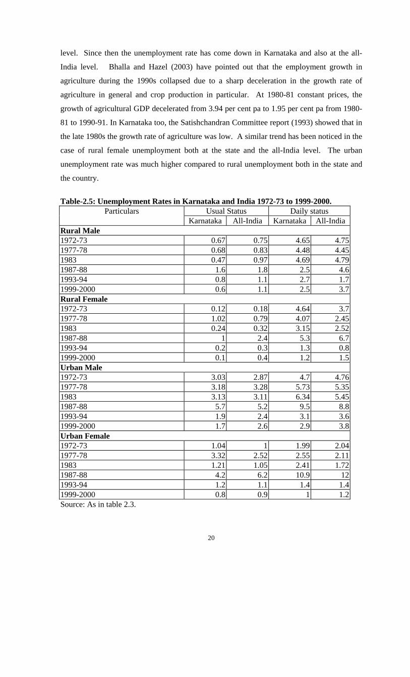
20

level. Since then the unemployment rate has come down in Karnataka and also at the all-

India level. Bhalla and Hazel (2003) have pointed out that the employment growth in

agriculture during the 1990s collapsed due to a sharp deceleration in the growth rate of

agriculture in general and crop production in particular. At 1980-81 constant prices, the

growth of agricultural GDP decelerated from 3.94 per cent pa to 1.95 per cent pa from 1980-

81 to 1990-91. In Karnataka too, the Satishchandran Committee report (1993) showed that in

the late 1980s the growth rate of agriculture was low. A similar trend has been noticed in the

case of rural female unemployment both at the state and the all-India level. The urban

unemployment rate was much higher compared to rural unemployment both in the state and

the country.

Table-2.5: Unemployment Rates in Karnataka and India 1972-73 to 1999-2000.

Usual Status Daily status Particulars Karnataka All-India Karnataka All-India

Rural Male 1972-73 0.67 0.75 4.65 4.751977-78 0.68 0.83 4.48 4.451983 0.47 0.97 4.69 4.791987-88 1.6 1.8 2.5 4.61993-94 0.8 1.1 2.7 1.71999-2000 0.6 1.1 2.5 3.7Rural Female 1972-73 0.12 0.18 4.64 3.71977-78 1.02 0.79 4.07 2.451983 0.24 0.32 3.15 2.521987-88 1 2.4 5.3 6.71993-94 0.2 0.3 1.3 0.81999-2000 0.1 0.4 1.2 1.5Urban Male 1972-73 3.03 2.87 4.7 4.761977-78 3.18 3.28 5.73 5.351983 3.13 3.11 6.34 5.451987-88 5.7 5.2 9.5 8.81993-94 1.9 2.4 3.1 3.61999-2000 1.7 2.6 2.9 3.8Urban Female 1972-73 1.04 1 1.99 2.041977-78 3.32 2.52 2.55 2.111983 1.21 1.05 2.41 1.721987-88 4.2 6.2 10.9 121993-94 1.2 1.1 1.4 1.41999-2000 0.8 0.9 1 1.2Source: As in table 2.3.

21

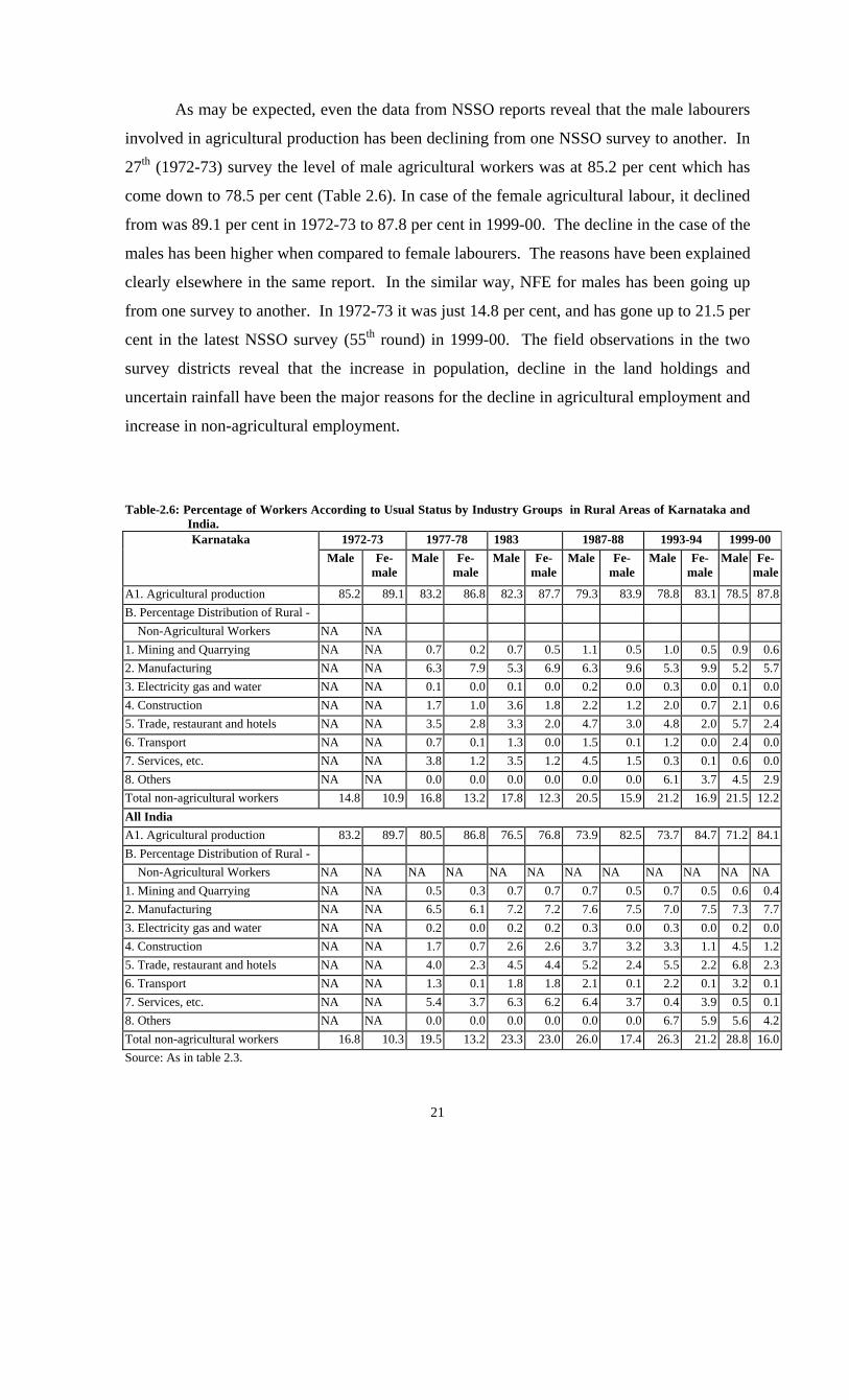
As may be expected, even the data from NSSO reports reveal that the male labourers

involved in agricultural production has been declining from one NSSO survey to another. In

27th (1972-73) survey the level of male agricultural workers was at 85.2 per cent which has

come down to 78.5 per cent (Table 2.6). In case of the female agricultural labour, it declined

from was 89.1 per cent in 1972-73 to 87.8 per cent in 1999-00. The decline in the case of the

males has been higher when compared to female labourers. The reasons have been explained

clearly elsewhere in the same report. In the similar way, NFE for males has been going up

from one survey to another. In 1972-73 it was just 14.8 per cent, and has gone up to 21.5 per

cent in the latest NSSO survey (55th round) in 1999-00. The field observations in the two

survey districts reveal that the increase in population, decline in the land holdings and

uncertain rainfall have been the major reasons for the decline in agricultural employment and

increase in non-agricultural employment.

Table-2.6: Percentage of Workers According to Usual Status by Industry Groups in Rural Areas of Karnataka and

India. 1972-73 1977-78 1983 1987-88 1993-94 1999-00 Karnataka

Male Fe-male

Male Fe-male

Male Fe-male

Male Fe-male

Male Fe-male

Male Fe-male

A1. Agricultural production 85.2 89.1 83.2 86.8 82.3 87.7 79.3 83.9 78.8 83.1 78.5 87.8B. Percentage Distribution of Rural - Non-Agricultural Workers NA NA 1. Mining and Quarrying NA NA 0.7 0.2 0.7 0.5 1.1 0.5 1.0 0.5 0.9 0.62. Manufacturing NA NA 6.3 7.9 5.3 6.9 6.3 9.6 5.3 9.9 5.2 5.73. Electricity gas and water NA NA 0.1 0.0 0.1 0.0 0.2 0.0 0.3 0.0 0.1 0.04. Construction NA NA 1.7 1.0 3.6 1.8 2.2 1.2 2.0 0.7 2.1 0.65. Trade, restaurant and hotels NA NA 3.5 2.8 3.3 2.0 4.7 3.0 4.8 2.0 5.7 2.46. Transport NA NA 0.7 0.1 1.3 0.0 1.5 0.1 1.2 0.0 2.4 0.07. Services, etc. NA NA 3.8 1.2 3.5 1.2 4.5 1.5 0.3 0.1 0.6 0.08. Others NA NA 0.0 0.0 0.0 0.0 0.0 0.0 6.1 3.7 4.5 2.9Total non-agricultural workers 14.8 10.9 16.8 13.2 17.8 12.3 20.5 15.9 21.2 16.9 21.5 12.2All India A1. Agricultural production 83.2 89.7 80.5 86.8 76.5 76.8 73.9 82.5 73.7 84.7 71.2 84.1B. Percentage Distribution of Rural - Non-Agricultural Workers NA NA NA NA NA NA NA NA NA NA NA NA 1. Mining and Quarrying NA NA 0.5 0.3 0.7 0.7 0.7 0.5 0.7 0.5 0.6 0.42. Manufacturing NA NA 6.5 6.1 7.2 7.2 7.6 7.5 7.0 7.5 7.3 7.73. Electricity gas and water NA NA 0.2 0.0 0.2 0.2 0.3 0.0 0.3 0.0 0.2 0.04. Construction NA NA 1.7 0.7 2.6 2.6 3.7 3.2 3.3 1.1 4.5 1.25. Trade, restaurant and hotels NA NA 4.0 2.3 4.5 4.4 5.2 2.4 5.5 2.2 6.8 2.36. Transport NA NA 1.3 0.1 1.8 1.8 2.1 0.1 2.2 0.1 3.2 0.17. Services, etc. NA NA 5.4 3.7 6.3 6.2 6.4 3.7 0.4 3.9 0.5 0.18. Others NA NA 0.0 0.0 0.0 0.0 0.0 0.0 6.7 5.9 5.6 4.2Total non-agricultural workers 16.8 10.3 19.5 13.2 23.3 23.0 26.0 17.4 26.3 21.2 28.8 16.0Source: As in table 2.3.

22

Growth of Workforce in the State and at the All India Level:

Chadha and Sahu (2002) have worked out the growth rates for the workforce by using

NSSO survey data for the years 1983 to 1993-94 and 1993-94 to 1999-00. Table-2.7

presents the same for Karnataka and all India. It can be seen from the table that in the first

period, 1983 to 1993-94, the growth rate in employment for rural and urban Karnataka was

2.12 and 2.95 per cent respectively. In the subsequent period, it was 0.17 and 2.54 for the

respective categories. This reveals the urban bias of policy makers. In real terms, one has to

try to increase rural employment, to reduce the regional disparities and urban migration.

Even at the all India level, the same trend prevails. Though there is a minor difference

between the usual status, weekly status and the daily status the trend has been the same

between the rural and the urban areas. Even then, as mentioned elsewhere, the urban

unemployment rate is high because of the increase in population due to migration from

villages to the urban centres.

Table-2.7: Growth of Total Workforce by Three Different Measures of Employment –

1983/1999-00. Karnataka Usual status Weekly status Daily status

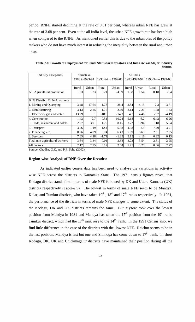
Rural Urban Total Rural Urban Total Rural Urban Total1983/1993-94 2.12 2.95 2.32 2.66 3.1 2.77 2.65 3.21 2.791993-94 to 1999-00 0.17 2.54 0.78 0.71 2.94 1.31 0.8 3.06 1.43All India 1983/1993-94 1.75 3.27 2.06 2.53 3.58 2.76 2.38 3.58 2.651993-94 to 1999-00 0.66 2.27 1.02 0.9 2.4 1.25 0.67 2.32 1.07Source: Chadha, G.K. and P.P. Sahu (2002). Table-2.8 presents the growth of employment for usual status for Karnataka and all

India across major industry categories. The table presents that the growth rate in employment

for agricultural production was positive from 1983 to 1993-94, whereas in the second period

it declined at the rate of 4.39 per cent for urban Karnataka. At the all India level, even for the

urban areas, the rate of agricultural employment high when compared to the rural areas.

However, in the latest period, the agricultural employment for the urban areas started

declining at the rate of 3.4 per cent. However, it is a welcome matter that in Karnataka, the

growth rate of agricultural employment is high in rural areas when compared to the urban.

In the first period, i.e., 1983 to 1993-94, the growth rate of NFE in the rural areas was

slightly higher when compared to urban NFE. in Karnataka state. In the subsequent study

23

period, RNFE started declining at the rate of 0.01 per cent, whereas urban NFE has grew at

the rate of 3.68 per cent. Even at the all India level, the urban NFE growth rate has been high

when compared to the RNFE. As mentioned earlier this is due to the urban bias of the policy

makers who do not have much interest in reducing the inequality between the rural and urban

areas.

Table-2.8: Growth of Employment for Usual Status for Karnataka and India Across Major Industry

Sectors.

Industry Categories Karnataka All India 1983 to1993-94 1993-94 to 1999-00 1983-1993-94 1993-94 to 1999-00

Rural Urban Rural Urban Rural Urban Rural Urban A1. Agricultural production 1.83 1.23 0.21 -4.39 1.38 1.54 0.18 -3.4

B. % Distribn. Of N-A workers 1. Mining and Quarrying 3.48 17.64 -1.78 -28.4 3.84 4.15 -2.3 -3.712. Manufacturing 3.13 2.25 -1.75 2.69 2.14 2.21 1.78 1.833. Electricity gas and water 13.29 8.1 -18.9 -14.3 4.7 4.46 -5.7 -4.194. Construction -1.43 2.7 0.51 10.24 5.18 6.2 6.43 6.265. Trade, restaurant and hotels 2.97 3.91 1.79 8.45 3.72 3.94 1.18 5.546. Transport 3.56 1.19 12.4 5.38 4.58 2.9 7.29 3.917. Financing, etc. 0.96 4.09 3.74 6.43 5.99 5.63 2.51 7.058. Services 7.65 4.18 -1.71 -1.32 3.13 4.16 0.32 0.13Total non-agricultural workers 3.54 3.34 -0.01 3.68 3.23 3.54 2.31 2.95All Sectors 2.12 2.95 0.17 2.54 1.75 3.27 0.66 2.27Source: Chadha, G.K. and P.P. Sahu (2002). Region-wise Analysis of RNE Over the Decades:

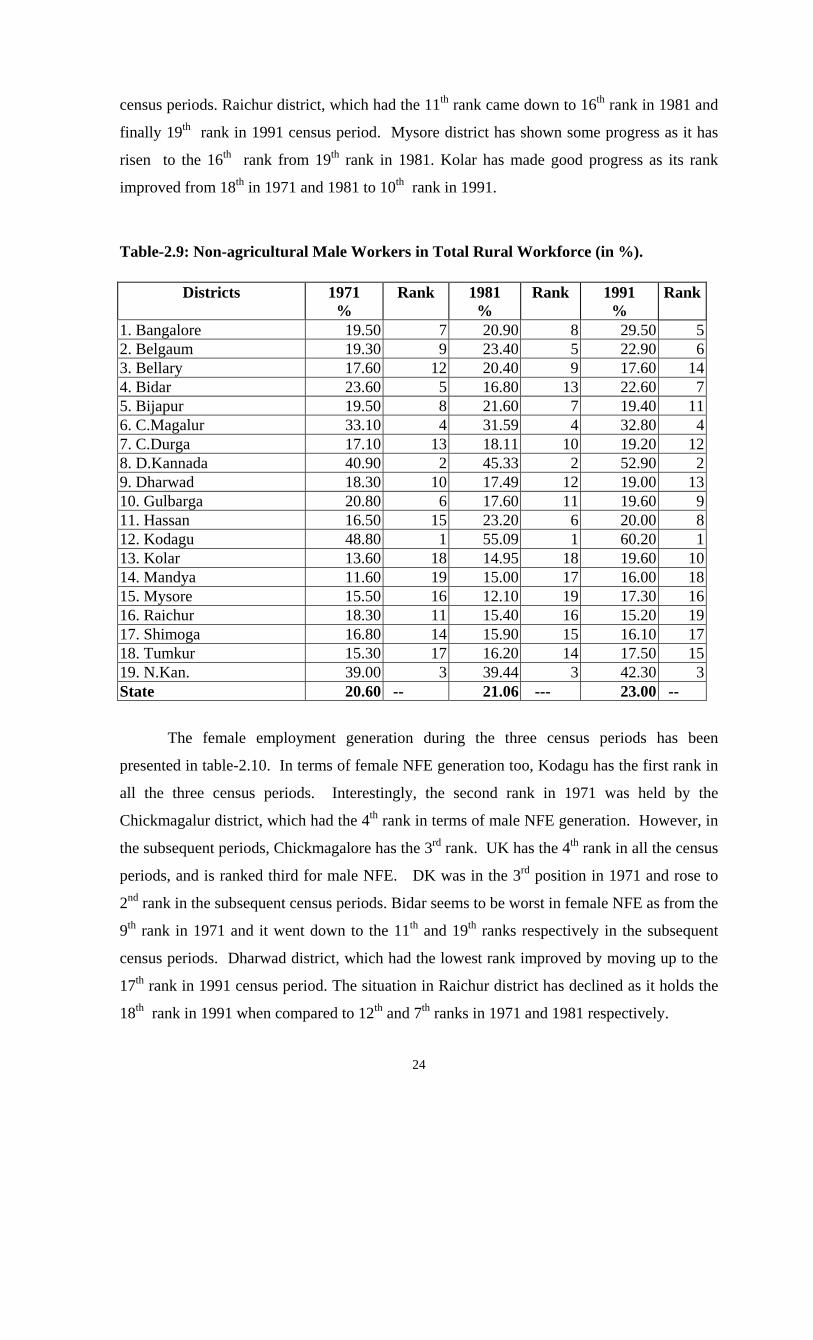
As indicated earlier census data has been used to analyse the variations in activity-

wise NFE across the districts in Karnataka State. The 1971 census figures reveal that

Kodagu district stands first in terms of male NFE followed by DK and Uttara Kannada (UK)

districts respectively (Table-2.9). The lowest in terms of male NFE seem to be Mandya,

Kolar, and Tumkur districts, who have taken 19th , 18th and 17th ranks respectively. In 1981,

the performance of the districts in terms of male NFE changes to some extent. The status of

the Kodagu, DK and UK districts remains the same. But Mysore took over the lowest

position from Mandya in 1981 and Mandya has taken the 17th position from the 19th rank.

Tumkur district, which had the 17th rank rose to the 14th rank. In the 1991 Census also, we

find little difference in the case of the districts with the lowest NFE. Raichur seems to be in

the last position, Mandya is last but one and Shimoga has come down to 17th rank. In short

Kodagu, DK, UK and Chickmagalur districts have maintained their position during all the

24

census periods. Raichur district, which had the 11th rank came down to 16th rank in 1981 and

finally 19th rank in 1991 census period. Mysore district has shown some progress as it has

risen to the 16th rank from 19th rank in 1981. Kolar has made good progress as its rank

improved from 18th in 1971 and 1981 to 10th rank in 1991.

Table-2.9: Non-agricultural Male Workers in Total Rural Workforce (in %).

Districts 1971 %

Rank 1981 %

Rank 1991 %

Rank

1. Bangalore 19.50 7 20.90 8 29.50 52. Belgaum 19.30 9 23.40 5 22.90 63. Bellary 17.60 12 20.40 9 17.60 144. Bidar 23.60 5 16.80 13 22.60 75. Bijapur 19.50 8 21.60 7 19.40 116. C.Magalur 33.10 4 31.59 4 32.80 47. C.Durga 17.10 13 18.11 10 19.20 128. D.Kannada 40.90 2 45.33 2 52.90 29. Dharwad 18.30 10 17.49 12 19.00 1310. Gulbarga 20.80 6 17.60 11 19.60 911. Hassan 16.50 15 23.20 6 20.00 812. Kodagu 48.80 1 55.09 1 60.20 113. Kolar 13.60 18 14.95 18 19.60 1014. Mandya 11.60 19 15.00 17 16.00 1815. Mysore 15.50 16 12.10 19 17.30 1616. Raichur 18.30 11 15.40 16 15.20 1917. Shimoga 16.80 14 15.90 15 16.10 1718. Tumkur 15.30 17 16.20 14 17.50 1519. N.Kan. 39.00 3 39.44 3 42.30 3State 20.60 -- 21.06 --- 23.00 --

The female employment generation during the three census periods has been

presented in table-2.10. In terms of female NFE generation too, Kodagu has the first rank in

all the three census periods. Interestingly, the second rank in 1971 was held by the

Chickmagalur district, which had the 4th rank in terms of male NFE generation. However, in

the subsequent periods, Chickmagalore has the 3rd rank. UK has the 4th rank in all the census

periods, and is ranked third for male NFE. DK was in the 3rd position in 1971 and rose to

2nd rank in the subsequent census periods. Bidar seems to be worst in female NFE as from the

9th rank in 1971 and it went down to the 11th and 19th ranks respectively in the subsequent

census periods. Dharwad district, which had the lowest rank improved by moving up to the

17th rank in 1991 census period. The situation in Raichur district has declined as it holds the

18th rank in 1991 when compared to 12th and 7th ranks in 1971 and 1981 respectively.

25

Table-2.10: Non-Agricultural Female Workers (in %)

1971 1981 1991 Districts % Rank % Rank % Rank

1. Bangalore 17.90 7 16.70 6 18.60 62. Belgaum 10.70 17 19.20 5 7.70 123. Bellary 12.60 13 10.40 9 7.30 134. Bidar 15.50 9 9.50 11 5.10 195. Bijapur 12.20 14 6.80 18 6.80 156. C.magalur 55.50 2 41.52 3 35.80 37. C.Durga 11.80 16 10.13 10 9.60 88. D.Kan. 29.90 5 46.52 2 57.10 29. Dharwad 9.80 19 6.80 19 6.60 1710. Gulbarga 17.10 8 6.90 17 6.70 1611. Hassan 34.40 3 11.60 8 18.70 512. Kodagu 57.00 1 59.02 1 62.10 113. Kolar 11.90 15 8.17 14 8.70 1114. Mandya 14.40 11 8.70 13 9.00 1015. Mysore 26.50 6 9.00 12 13.40 716. Raichur 13.20 12 14.50 7 5.40 1817. Shimoga 10.50 18 7.00 16 7.10 1418. Tumkur 15.20 10 8.00 15 9.60 919. U.Kan. 30.90 4 28.77 4 25.00 4State 19.20 -- 16.61 --- 14.80 --- Source: As in table 2.1

The non-agricultural workers in the total rural workforce has been presented in Table-

2.11. The table reveals that when both male and female non-agricultural workers are

combined we find little variation in terms of the performance of the districts. As usual

Kodagu takes first rank in having more non-agricultural workers out of the total rural

workforce in all the three census periods. The second place was held DK in 1981 and 1991

census periods and in the 1971 census it had the third place. In the 1971 census period

Chickmagalur had the 2nd position, which has come down to third position in the subsequent

census periods. The UK district has maintained the 4th rank in all the census periods. Kolar

district was the lowest in terms of NFE in 1971, a position it subsequently improved to the

17th and 10th ranks. Mandya, which had the 18th rank in 1971 improved to 16th rank

subsequently. Raichur district, which had the 11th and 9th rank in 1971 and 1981 came down

to the 19th rank in 1991. The total RNFE in the state accounted for about 19.90, 18.84 and

18.90 per cent in the 1971, 1981 and 1991 census periods respectively. This clearly shows

that RNFE has not made any progress over the period under study in the state.

26

Table-2.11: Percentage of Non-Agricultural Workers in Total Rural Workforce

1971 1981 1991 Districts % Rank % Rank % Rank

1. Bangalore 18.70 9 18.80 6 24.05 52. Belgaum 15.00 14 21.30 5 15.30 83. Bellary 15.10 13 15.40 8 12.45 174. Bidar 19.55 7 13.15 12 13.85 115. Bijapur 15.85 10 14.20 10 13.10 146. C.Magalur 44.30 2 36.56 3 34.30 37. C.Durga 14.45 15 14.12 11 14.40 98. D.Kannada 35.40 3 45.93 2 55.00 29. Dharwad 14.05 16 12.15 14 12.80 1510. Gulbarga 18.95 8 12.25 13 13.15 1311. Hassan 25.45 5 17.40 7 19.35 612. Kodagu 52.90 1 57.06 1 61.15 113. Kolar 12.75 19 11.56 17 14.15 1014. Mandya 13.00 18 11.85 16 12.50 1615. Mysore 21.00 6 10.55 19 15.35 716. Raichur 15.75 11 14.95 9 10.30 1917. Shimoga 13.65 17 11.45 18 11.60 1818. Tumkur 15.25 12 12.10 15 13.55 1219. N.Kan. 34.95 4 34.11 4 33.65 4State. 19.90 --- 18.84 ---- 18.90 ---- Rural NFE And Industry Categories. An effort has been made to study NFE generation across various industry categories

to understand exactly which industry category has major scope for NFE. For the analysis we

have taken the district-wise data from the three census periods from 1971 to 1991. Table-

2.12 presents the activity-wise distribution of male and female workers during the 1971

census. On the whole, RNFE has been high in three sectors viz., allied agricultural activities,

other services and manufacturing in household sectors. Chickmagalur, Hassan, Kodagu, UK,

Kolar and Tumkur are the districts where we find a lot of RNFE in allied activities. Among

these, in the coastal Malnad districts like Chikmagalur, DK, Hassan, Kodagu, Shimoga, and

UK the percentages are high. This may be due to the availability of forest resources and sea

products in abundance. Female labourers seem to be employed more in allied activities and

manufacturing of HH and non-HH industries. The lowest sector for both males and females

seems to be mining and quarrying and especially for female, the figures are not encouraging

even in construction and transport and commerce. In the case of cultivators and agricultural

labourers, generally the employment rate is very high, about 80 per cent for males and 81 per

27

cent for females at the state level. Among the districts DK, Kodagu and UK are the districts,

which with the lowest number of cultivators and agricultural labourers. The sample district,

Raichur is much above the state average in terms of cultivators and agricultural labourers and

the NFE is low when compared to the state average excepting for trade. Whereas, Kodagu,

DK and UK have been better in all respects when compared to the state average.

Table-2.12: Activity-wise Distribution of Male and Female Workers in 1971 (in %)

Cultivators & agri.lab.

Allied Agri. Acti.

Mining & Quarrying

Manufac-turing (HH)

Manufac- turing (NHH)

Construction Trade Transport & Commerce

Other services

Districts

M FM M FM M FM M FM M FM M FM M FM M FM M FM

1. Bangalore 80.70 82.10 2.40 4.00 0.10 0.20 2.10 2.50 5.30 3.10 1.00 1.00 2.20 2.20 1.00 0.50 5.40 4.42. Belgaum 80.70 89.40 2.70 1.80 0.10 0.00 4.50 4.10 2.50 0.70 1.50 0.90 2.50 1.20 0.70 0.20 4.80 1.83. Bellary 82.30 87.40 1.90 0.70 2.50 2.90 2.50 2.60 1.30 0.60 1.10 0.50 2.30 1.50 1.40 1.00 4.60 2.84. Bidar 76.40 84.40 4.70 1.30 0.30 0.10 3.40 3.00 2.10 0.60 1.20 0.10 3.90 0.50 0.50 0.00 7.50 9.95. Bijapur 80.30 87.80 4.20 2.20 0.20 0.10 5.20 4.80 1.20 0.40 1.00 0.40 2.50 1.50 0.80 0.70 4.40 2.16. C.Magalur 67.00 44.50 16.20 39.30 0.70 0.70 1.60 1.10 2.10 0.80 1.30 0.90 2.80 0.70 0.50 0.00 7.90 127. C.Durga 82.90 88.10 4.90 2.10 0.20 0.40 2.80 3.40 1.80 0.80 1.10 0.90 2.00 1.80 0.40 0.00 3.90 2.48. D.Kannada 59.20 70.00 6.50 1.90 0.30 0.10 8.00 16.90 6.40 4.90 2.20 0.20 7.30 2.10 2.30 0 7.90 3.89. Dharwad 81.60 90.20 2.60 1.00 0.30 0.30 4.20 3.20 1.40 0.70 0.70 0.20 3.80 1.70 0.70 0.30 4.60 2.410. Gulbarga 79.00 82.80 3.90 1.00 0.50 0.60 3.30 3.90 2.20 1.30 1.50 1.00 2.90 1.30 0.60 0.00 5.90 811. Hassan 83.40 65.60 5.70 20.60 0.20 0.30 1.50 2.70 1.30 1.30 2.10 3.20 1.30 0.90 0.50 0.10 3.90 5.312. Kodagu 51.10 42.70 26.00 42.60 0.40 0.30 1.70 1.30 2.50 1.00 2.90 1.80 4.30 0.30 0.80 0.00 10.20 9.713. Kolar 86.40 88.20 3.50 5.90 0.30 0.00 1.60 1.20 1.70 0.90 0.60 0.50 2.10 1.40 0.50 0.20 3.30 1.814. Mandya 88.40 85.50 1.20 3.10 0.10 0.1 2.00 2.50 1.70 1.00 0.50 0.30 1.60 1.50 0.30 0.00 4.20 5.915. Mysore 84.50 73.20 2.40 3.70 0.20 0.30 2.10 4.10 1.90 2.40 1.80 4.30 1.90 1.70 0.30 0.00 4.90 1016. Raichur 81.60 86.70 3.30 2.20 0.80 0.10 3.20 3.30 1.70 0.80 1.00 0.30 2.70 1.40 0.50 0.30 5.10 4.817. Shimoga 83.20 89.30 4.10 3.70 0.10 0.20 2.70 1.70 1.50 1.20 1.30 0.80 2.60 1.40 0.50 0.00 4.00 1.518. Tumkur 84.60 84.80 3.90 3.80 0.30 0.20 2.90 4.30 1.20 0.80 0.90 0.90 1.90 1.90 0.40 0.10 3.80 3.219. N.Kan. 61.00 69.10 16.80 11.30 1.40 2.80 2.70 1.90 3.00 2.30 1.40 1.30 3.40 2.80 2.60 1.40 7.70 7.1State 79.50 80.80 4.60 4.90 0.40 0.40 3.30 5.10 2.30 1.60 1.30 0.90 2.80 1.60 0.80 0.30 5.10 4.4

Note: 1) M = Male, FM = Female 2) HH = Household Source: Census Report 1971

28

During the 1981 census also a similar trend has been observed. However, there is an

improvement in mining and quarrying, commerce, trade and also construction (Table 2.13).

The sample district, Raichur, has made significant progress in terms of NFE. For instance, it

had more NFE in the case of trade in 1971 when compared to the state average. Whereas by

1981 some progress has been made in the manufacturing of NHH (female NFE),

construction, trade, transport (male NFE) and also other services. For all these variables,

Raichur district changed positively. DK has also made more progress in terms of generating

NFE when compared to the state average. In 1981 census also, DK, UK and Kodagu stood

first in terms of NFE generating districts in the state. In general the male cultivators and

agricultural labourers have come down whereas the female percentage has gone up when

compared to the 1971 census at the state level.

Table-2.13: Activity-wise Distribution of Male and Female Workers in 1981 (in %)

Cultivators & agri.lab.

Allied Agri. Acti.

Mining & Quarrying

Manufac-turing (HH)

Manufact-uring

(NHH)

Construction Trade Transport & Commerce

Other servicesDistricts

M FM M FM M FM M FM M FM M FM M FM M FM M FM

1. Bangalore 78.90 83.40 4.60 4.00 0.40 0.40 2.80 5.30 3.50 2.80 1.30 0.60 3.20 1.50 1.10 0.20 4.00 1.9

2. Belgaum 76.70 80.90 3.00 3.20 0.20 0.30 2.00 2.40 7.40 5.00 1.40 1.70 2.90 2.50 1.50 0.50 5.00 3.6

3. Bellary 79.60 89.60 2.50 1.20 0.10 0.00 3.80 3.80 4.30 1.80 1.70 0.50 3.20 1.50 1.10 0.10 3.70 1.5

4. Bidar 83.10 90.50 1.70 0.40 2.60 2.20 2.40 2.20 2.00 1.10 0.90 0.20 2.80 2.00 0.90 0.10 3.50 1.3

5. Bijapur 78.40 93.30 4.00 0.30 0.10 0.00 2.40 1.80 3.70 1.60 1.30 0.10 4.10 0.60 1.50 0.30 4.50 2.1

6. C.Magalur 68.42 58.48 18.89 35.83 0.13 0.00 1.78 1.30 1.81 0.46 0.98 0.45 3.12 1.13 0.95 0.31 3.93 2.04

7. C.Durga 81.88 89.86 4.32 1.55 0.39 0.26 2.80 3.29 2.64 1.20 0.88 0.23 2.78 1.81 0.67 0.05 3.63 1.74

8. D.Kannada 54.67 53.44 7.92 1.23 0.22 0.07 7.29 29.98 10.19 12.91 1.80 0.07 8.15 0.67 3.77 0.29 5.99 1.3

9. Dharwad 82.50 93.19 2.23 0.36 0.21 0.24 3.78 2.85 2.37 0.88 0.90 0.17 3.36 1.12 0.96 0.02 3.68 1.16

10. Gulbarga 82.50 93.20 2.20 0.40 0.20 0.20 3.80 2.90 2.40 0.90 0.90 0.20 3.40 1.10 1.00 0.00 3.70 1.2

11. Hassan 76.80 88.30 5.70 1.70 1.30 1.40 2.80 2.30 2.90 1.30 2.60 1.40 3.40 1.60 0.80 0.10 3.70 1.8

12. Kodagu 44.91 40.98 35.09 49.64 0.04 0.05 1.06 0.56 3.75 1.18 2.18 1.00 5.00 0.78 1.83 0.40 6.14 5.41

13. Kolar 84.84 91.30 3.21 3.44 0.41 0.05 1.13 0.26 2.49 1.35 0.73 0.12 2.53 1.29 0.83 0.26 3.62 1.4

14. Mandya 84.80 91.30 3.20 3.40 0.40 0.00 1.30 0.80 2.50 1.40 0.70 0.10 2.50 1.30 0.80 0.30 3.60 1.4

15. Mysore 87.90 91.10 1.20 0.90 0.00 0.00 1.60 1.80 2.70 1.60 0.70 0.50 2.10 2.00 0.40 0.00 3.40 2.2

16. Raichur 84.60 85.60 2.70 2.80 0.10 0.10 1.70 2.20 3.30 3.40 1.40 1.50 2.40 1.60 0.60 0.30 3.20 2.6

17. Shimoga 84.10 93.00 2.10 0.70 0.50 0.00 2.60 2.10 2.40 1.20 1.60 0.30 3.00 1.20 0.50 0.10 3.20 1.4

18. Tumkur 83.80 91.90 2.70 1.00 0.40 0.50 2.00 1.50 2.80 1.60 1.00 0.30 3.10 1.10 0.70 0.10 3.50 1.9

19. N.Kan. 60.56 71.23 15.22 7.45 1.79 1.71 2.69 1.72 4.66 4.10 2.08 2.99 4.32 5.21 3.39 0.91 5.29 4.68

State 78.94 83.40 4.64 3.99 0.42 0.39 2.84 5.32 3.52 2.81 1.34 0.57 3.22 1.46 1.13 0.18 3.95 1.89

Source: Census Report 1981.

29

In the 1991 census period too NFE was high in the case of the allied agricultural

activities, manufacturing of non-household industries, trade and other services (table-2.14) .

However, in case of all the other sectors also there is an improvement. Interestingly the

percentage of male cultivators and agricultural labourers has come down but female

involvement in these sectors has gone up from the 1971 to 1991 census. In 1971 the male

percentage was 79.50 but it has come down to 77.10 per cent. In case of females the

percentage in 1971 was 80.80 but it has increased to 85.20 per cent. The same three districts,

DK, UK and Kodagu have fewer cultivators and agricultural labourers and they have more

NFE. In Raichur district, the percentage of cultivators and agricultural labourers has gone up

over a period of time and the NFE has come down. Table-2.14:Activitywise Distribution of Male and Female Workers in 1991 (in %).

Cultivators & agri.lab.

Allied Agri. Acti.

Mining & Quarrying

Manufac- turing (HH)

Manufac- Turing (NHH)

Construction Trade Transport & Commerce

Other services

Districts

M FM M FM M FM M FM M FM M FM M FM M FM M FM

1. Bangalore 70.70 81.40 3.30 2.50 1.60 1.80 1.40 2.00 8.50 5.70 1.90 0.80 4.20 2.20 2.20 0.10 6.40 3.5

2. Belgaum 77.20 92.30 2.00 0.60 0.20 0.10 2.90 2.40 4.20 1.10 2.30 0.20 3.70 1.20 1.40 0.00 6.20 2.1

3. Bellary 82.40 92.80 1.90 0.30 2.00 1.20 1.40 1.00 1.70 0.70 1.10 0.10 3.90 1.80 1.20 0.20 4.40 2

4. Bidar 77.40 95.00 1.70 0.20 0.60 0.20 1.50 0.80 2.70 0.50 1.60 0.20 5.50 0.50 2.30 0.10 6.70 2.6

5. Bijapur 80.80 93.10 2.30 0.60 0.40 0.10 3.10 1.90 2.50 1.00 1.50 0.10 3.40 1.20 1.10 0.00 5.10 1.9

6. C.Magalur 67.30 64.30 16.00 28.00 0.40 0.30 0.90 1.00 2.30 1.10 1.50 0.50 4.50 1.10 1.10 0.10 6.10 3.77. C.Durga 80.80 90.30 3.40 1.00 0.50 0.30 1.90 2.20 2.60 1.10 1.20 0.20 3.90 2.00 0.90 0.00 4.80 2.8

8. D.Kannada 47.20 42.90 11.10 3.10 0.70 0.20 1.50 0.90 10.90 46.70 3.50 0.30 11.30 1.60 4.40 0.10 9.50 4.2

9. Dharwad 81.10 93.40 1.90 0.30 0.30 0.10 2.20 1.40 3.10 1.20 1.10 0.10 4.50 1.10 1.30 0.00 4.60 2.4

10. Gulbarga 80.50 93.10 3.10 0.70 1.50 1.00 1.80 1.10 1.70 0.40 1.30 0.20 4.00 1.10 1.10 0.00 5.10 2.2

11. Hassan 80.20 81.40 6.70 12.30 0.60 0.40 0.70 0.80 2.00 1.00 1.20 0.50 3.00 1.00 1.30 0.00 4.50 2.7

12. Kodagu 39.90 37.80 38.00 51.80 0.40 0.50 0.60 0.40 3.10 1.50 2.10 0.50 5.50 1.00 2.00 0.10 8.50 6.3

13. Kolar 80.30 91.30 4.30 2.60 0.90 0.20 0.90 0.80 2.90 1.40 1.20 0.20 3.80 1.30 1.20 0.00 4.40 2.2

14. Mandya 84.10 90.90 2.90 2.00 0.60 0.60 0.80 0.80 2.70 0.80 1.00 0.70 3.10 1.70 0.70 0.00 4.20 2.4

15. Mysore 82.60 86.60 3.50 3.00 0.60 0.50 1.10 2.00 3.00 2.80 1.50 0.50 3.50 1.90 0.70 0.00 3.40 2.7

16. Raichur 84.90 94.60 1.50 0.40 0.50 0.20 1.90 1.30 1.30 0.40 0.60 0.10 3.40 1.10 0.60 0.00 5.40 1.9

17. Shimoga 83.90 92.70 2.50 0.70 0.40 0.40 1.40 1.20 2.20 0.80 0.80 0.10 3.80 1.10 0.90 0.00 4.10 2.8

18. Tumkur 82.50 90.50 2.80 1.10 0.50 0.20 1.90 2.60 2.30 1.60 1.00 0.20 3.30 1.60 0.90 0.00 4.80 2.3

19. N.Kan. 57.70 74.90 17.40 7.60 1.50 1.10 1.80 1.10 3.70 1.40 3.10 0.80 5.90 5.30 2.30 0.50 6.60 7.2

State 77.10 85.20 4.60 3.30 0.70 0.40 1.70 1.50 3.50 5.00 1.50 0.30 4.30 1.50 1.40 0.10 5.30 2.7

Source: Census Report 1991.

30

Determinants of Rural Non-Farm Employment: We have taken few variables relating to agriculture and infrastructure and try to

see the impact of these on the rural workforce across various district groups. Towards

these we have classified the districts into four groups based on the status of NFE. The

respective groups are 1) Very High NFE Districts, 2) High NFE Districts, 3) Medium

NFE districts and 4) Low NFE Districts. We have utilised the census data towards the

same. In 1971 area under forest, irrigated area and the literacy rate play a major role to

determine the NFE. The area under forest has positive impact on the NFE. As the area

under forest increases the NFE also increase and vice-versa (Table 2.15). The area under

irrigation has the negative relationship with NFE. As the percentage of the irrigated area

increases the NFE decreases and vice-versa. And finally the literary rate has the positive

impact on the NFE. The table reveals that the districts where the NFE is high the literacy

rate is high and the districts where the literary rate is low the NFE is low.

Table-2.15: Development of Agriculture and Infrastructure Vis-à-vis NFE (1971) Degree of Non-Farm

Employment

% of Cultiva-tors and agricul-

tural labourers

Work force in

non-farm sector

% Of Forest area to

total geo-graphical

area

% Of net sown area

to total geogra-

phical area

% Of irrigated

area to net sown area

Literacy rate

Road length per thousand population

Railway length per thousand

population

RNFE Very High

67.57 27.19 30.03 39.62 14.38 33.36 1.87 0.06

RNFE High 77.18 19.38 17.57 50.37 12.71 32.02 1.46 0.11

RNFE Medium

85.17 16.45 8.75 62.07 16.16 30.96 1.70 0.10

RNFE Low 89.35 10.63 6.22 48.93 21.15 27.97 2.16 0.10

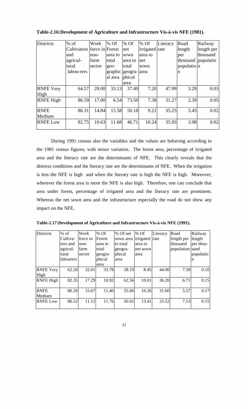
Even in 1981 the variables like the forest area, percentage of irrigated area and the

literacy rate have been the determinants of NFE in rural areas. However in case of the

second category of the districts where the NFE is high the area under forest is low when

compared to the other two categories like medium and low NFE districts. It is highly

difficult to reason it out why the results behave like this. However the other two

variables are behaving according to the earlier case (Table 2.16).

31

Table-2.16:Development of Agriculture and Infrastructure Vis-à-vis NFE (1981). Districts % of

Cultivators and agricul-tural labou-rers

Work force in non-farm sector

% Of Forest area to total geo-graphical area

% Of net sown area to total geogra-phical area

% Of irrigated area to net sown area

Literacy rate

Road length per thousand population

Railway length per thousand population

RNFE Very High

64.57 29.00 33.13 37.49 7.20 47.99 3.29 0.03

RNFE High 86.59 17.00 6.54 73.50 7.38 31.27 2.39 0.05

RNFE Medium

86.31 14.84 15.58 50.18 9.21 35.25 3.45 0.02

RNFE Low 82.75 10.63 11.68 46.71 10.24 35.93 3.98 0.02

During 1991 census also the variables and the values are behaving according to

the 1981 census figures, with minor variation. The forest area, percentage of irrigated

area and the literacy rate are the determinants of NFE. This clearly reveals that the

distress conditions and the literacy rate are the determinants of NFE. When the irrigation

is less the NFE is high and when the literary rate is high the NFE is high. Moreover,

wherever the forest area is more the NFE is also high. Therefore, one can conclude that

area under forest, percentage of irrigated area and the literacy rate are prominent.

Whereas the net sown area and the infrastructure especially the road do not show any

impact on the NFE.

Table-2.17:Development of Agriculture and Infrastructure Vis-à-vis NFE (1991). Districts % of

Cultiva-tors and agricul-tural labourers

Work force in non-farm sector

% Of Forest area to total geogra-phical area

% Of net sown area to total geogra-phical area

% Of irrigated area to net sown area

Literacy rate

Road length per thousand population

Railway length per thou-sand population

RNFE Very High

62.20 32.01 33.78 38.19 8.45 44.00 7.58 0.10

RNFE High 82.35 17.29 10.92 62.56 10.01 36.20 6.71 0.15

RNFE Medium

86.26 15.67 11.40 55.06 10.26 31.60 5.57 0.17

RNFE Low 86.52 11.12 11.76 50.92 13.41 33.52 7.53 0.15

32

CHAPTER III

NON-FARM EMPLOYMENT IN THE SAMPLE DISTRICTS – SECONDARY DATA ANALYSIS

This chapter includes three sections. The first section deals with the basic socio-

economic indicators of the sample districts and of Karnataka state, the second section

deals with category-wise employment generation based on census data and the final

section deals with the determinants of RNFE at the district level.

Section-1

Socio-Economic Details of the Selected Districts

To understand the nature of the sample districts we have tried to gather a detailed

information of the districts (Table 3.1). We start with total geographical area and end

with a host of relevant variables so that they indicate the socio-economic position of the

sample districts. Out of 25 variables which seem to be the determinants of RNFE, we

found that around 72 per cent of the determinants were favourable in DK when compared

to Raichur district where only around 28 per cent are favourable for RNFE. Again out of

18 variables which are favourable for RNFE generation, 61.11 per cent have strong

features of NFE. These are strong indications to say that DK is in a more advantageous

position to generate more NFE when compared to Raichur district. Therefore, NFE is

not only due to distress factors and also development of the area in terms of literacy and

infrastructure.

33

Table-3.1: Socio-Economic Parameters of the Sample Districts Particulars Ref. Year DK Raichur State

Total geographical area (in lakh ha) 1998-99 2.505 4.388 190.50% of pop.of the distcs to the state (Popn in lakhs) 2001 3.596 3.126 527.34Annual growth rate of population in % 1991-01 1.40 2.20 1.70Population density per sq.km 2001 416 241 275Proportion of rural to total population 2001 61.58 74.57 66.01Sex ratio(number of females per 1000 males) 2001 1023 980 964SC/ST population(%) to total population 1991 10 25 20.64Literacy rate for the entire population (%) 2001 83.47 49.54 67.04Male literacy rate 2001 89.74 62.02 76.29Female literacy rate 2001 77.39 36.84 57.45Rural literacy rate % (Persons) 1991 72 30 48Rural literacy rate % (Male)) 1991 82 44 60Rural literacy rate % (Female) 1991 64 16 35Rural literacy rate % (Persons) 2001 79.93 43.15 59.68Proportion of area under forests 1998-99 26.92 2.17 16.07Land not available for cultivation (%) 1998-99 24.02 4.86 10.99Other uncultivated land (%) 1998-99 22.07 29.32 17.86Average Rainfall(Normal in mms) 1901-70 3975 631 1139Proportion of Net sown area 1998-99 26.96 63.63 55.06Average size of land holdings (ha) 1995-96 1.05 2.63 1.94Proportion of net irrigated area to NSA 1998-99 51.3 23.64 23.75Cropping intensity 1998-99 124.5 121.12 117.37Village roads (kms) 1998-99 1269 996 48148% of HH having electricity 1991 42.4 32.5 52.5% of rural HH having electricity 1991 31.55 26.46 42.89No. of cities 1991 1 1 18Average size of cities 1991 281161 170577 416714No. of towns 1991 26 12 288No. of villages 1991 615 1369 27066Average size of village 1991 3140 1369 1147Livestock per 1000 human population 1997 348.48 763.99 600.27Vocational edcnl.institutions per lakh popln. 1993-94 0.72 0.93 1.23Vocational edcnl.institutions per lakh popln. 2000-01 NA NA 1.21% of agricultural labourers in total workforce 2001 4.43 45 26.39% of cultivators in total workforce 2001 5.23 28.35 29.48No of Tractors per 1000 ha NSA 1997 1.31 3.19 7.74No of pumpsets per 1000 ha NSA 1997 109.21 10.38 58.43Poverty ratio in Karnataka 1999-00 NA NA 20.04Poverty ratio (Rural) 1999-00 NA NA 17.38Poverty ratio (Urban) 1999-00 NA NA 25.25Sources: 1) Karnataka at a Glance – 2001-02. 2) Livestock Census 1997. 3) Censuses 1991 and 2001.

Section – II

Status of Non-Farm Employment in the Sample Districts

To find out the status of RNFE in the sample districts we have used census data

from 1961 to 1991. We have given the total RNFE, and male and female RNFE

separately. Table 3.2, presents the details of NFE in the sample districts. Interestingly, it

34

is found that altogether, Raichur has more cultivators and agricultural labourers when

compared to DK. The number of females engaged in cultivation and labour work has

been high compared to males in both the districts, and vice-versa in the case of NFAs.

Among the NFAs, other services and manufacturing in household industry seems to rank

highest compared to any other activity. DK has more NFE compared to Raichur district.

In the 1971 census it was seen that the percentage of cultivators and agricultural

labourers came down for DK when compared to the 1961 census, whereas for the

Raichur district it went up. This clearly reveals that the NFE increased in 1971 for DK

and declined for Raichur district. In 1971, the allied agricultural activities,

manufacturing in HH and non-HH industries, transport and communication and other

services are the industry categories where NFE was high. In most of the sectors, the

percentage of NFE was high for DK when compared to the Raichur district. In the 1971

census, the percentage of women involved in cultivation and agricultural labour is high

when compared to that of males. Female NFE seems to be moderately good in case of

allied agricultural activities, manufacturing in HH and non-HH industry and other

services. However, they are lower when compared to the males.

By the 1981 census, both for Raichur district and the state, the percentage of

cultivators and the agricultural labourers in general, and for females in particular, went

up, whereas for the DK district it came down when compared to the 1971 census. The

decline in the female percentage in agriculture and its labour was absorbed by the

manufacturing in HH and non-HH sector in DK. The percentage of female NFE in the

above sectors is 29.98 and 12.91 per cent respectively, which is very high compared to

their male counterparts. In all the other activities DK has more NFE compared to the

Raichur district.

Coming to the 1991 census we found that the percentage of cultivators and

agricultural labourers has gone up further in Raichur district and came down further for

DK district. This held good for both males and females in both the districts. Even here

female NFE is low when compared to that of males in DK district. Manufacturing in the

HH industry has come down markedly for both males and females. In Raichur, the major

non-farm activities seem to be other services and trade and commerce for males and for

females it is other services and manufacturing in HH industry.

35

Table-3.2: Rural Male and Female NFE in the Sample Districts (in %)

1961 Rural employment Male R.Emp. Female R.Emp.

Industry categ. Raichur DK State Raichur DK State Raichur DK State Culti & Agril Lab. 82.61 73.55 81.01 81.21 65.13 78.73 85.10 82.57 84.86

IV. M & Q. 0.00 0.00 0.00 0.00 0.00 0.00 0.00 0.00 0.00In.MQLFF 0.51 3.85 3.23 0.71 5.87 3.62 0.17 1.69 2.57Va.HHI 6.45 6.44 5.88 7.08 6.34 6.11 5.33 6.55 5.50Vb.NHHI 0.28 4.62 1.22 0.29 6.06 1.55 0.26 3.07 0.67VI. Contn. 0.69 0.75 0.99 0.84 1.34 1.26 0.42 0.13 0.54VII. T&C. 1.67 3.16 1.75 2.00 4.12 2.08 1.08 2.13 1.18VIII. TS&C. 0.21 0.76 0.27 0.32 1.47 0.43 0.01 0.01 0.01IX. Otrs. 7.58 6.86 5.65 7.56 9.68 6.23 7.62 3.84 4.66Total 100 100 100 100 100 100 100 100 1001971 Culti & Agril Lab. 82.80 63.5 79.80 81.60 59.20 79.50 86.70 70.00 80.80Allied Agri.Act. 3.00 4.6 4.70 3.30 6.50 4.60 2.20 1.90 4.90IV. M & Q. 0.70 0.20 0.40 0.80 0.30 0.40 0.10 0.10 0.40Va.HHI 3.20 11.60 3.70 3.20 8.00 3.30 3.30 16.90 5.10Vb.NHHI 1.50 5.80 2.10 1.70 6.40 2.30 0.80 4.90 1.60VI. Contn. 0.90 1.40 1.20 1.00 2.20 1.30 0.30 0.20 0.90VII. T&C. 2.40 5.20 2.50 2.70 7.30 2.80 1.40 2.10 1.60VIII. TS&C. 0.40 1.40 0.70 0.50 2.30 0.80 0.30 0 0.30IX. Otrs. 5 6.2 5 5.10 7.90 5.10 4.8 3.8 4.4Total 100 100 100 100 100 100 100 100 1001981 Culti & Agril Lab. 84.80 54.15 81.17 84.60 54.67 78.94 85.60 53.44 83.40Allied Agri.Act. 2.70 5.08 13.40 2.70 7.92 15.20 2.80 1.23 7.40IV. M & Q. 0.10 0.15 1.80 0.10 0.22 1.80 0.10 0.07 1.70Va.HHI 1.80 16.92 2.50 1.70 7.29 2.70 2.20 29.98 1.70Vb.NHHI 3.30 11.34 4.50 3.30 10.19 4.70 3.40 12.91 4.10VI. Contn. 1.40 1.07 2.30 1.40 1.80 2.10 1.50 0.07 3.00VII. T&C. 2.30 4.98 4.50 2.40 8.15 4.30 1.60 0.67 5.20VIII. TS&C. 0.50 2.30 2.80 0.60 3.77 3.40 0.30 0.29 0.90IX. Otrs. 3.1 4.02 5.1 3.20 5.99 5.30 2.6 1.34 4.7Total 100 100 100 100 100 100 100 100 1001991 Culti & Agril Lab. 88.70 45.30 79.70 84.90 47.20 77.10 94.60 42.90 85.20Allied Agri.Act. 1.10 7.70 4.20 1.50 11.10 4.60 0.40 3.10 3.30IV. M & Q. 0.30 0.40 0.60 0.50 0.70 0.70 0.20 0.20 0.40Va.HHI 1.70 1.20 1.60 1.90 1.50 1.70 1.30 0.90 1.50Vb.NHHI 0.90 26.00 4.00 1.30 10.90 3.50 0.40 46.70 5.00VI. Contn. 0.40 2.10 1.10 0.60 3.50 1.50 0.10 0.30 0.30VII. T&C. 2.50 7.20 3.40 3.40 11.30 4.30 1.10 1.60 1.50VIII. TS&C. 0.40 2.60 0.90 0.60 4.40 1.40 0.00 0.10 0.10IX. Otrs. 4 7.3 4.5 5.40 9.50 5.30 1.9 4.2 2.7Total 100 100 100 100 100 100 100 100 100Source: Census Reports 1961, 1971, 1981 and 1991.

36

It can be concluded from the above discussion that the percentage of cultivators

and agricultural labourers is increasing in Raichur district but NFE has gone down to

some extent. In comparison, in DK district, the percentage of cultivators and agricultural

labourers has come down and NFE has gone up. In general, women’s involvement in

cultivation and agricultural labour activities is more and the percentage has been

increasing over a period of time in Raichur district.

Determinants of Non-Farm Employment in Karnataka:

In this section, NFE in Karnataka has been analysed for the two census periods,

viz., 1981 and 1991. For the earlier census periods, it is highly difficult to get the data for

the variables mentioned below. From the 2001 census, detailed data has not yet been

published. The task of analysing factors responsible to variations in NFE at district level

is, however, not very easy. This is mainly because of data problems. There are data

limitations regarding some of the variables used, especially per-capita income at the

district level and the proportion of marginal holdings to total holdings. In view of these

factors, the analysis may not be very satisfactory; however, given the non-availability of

data, we have to use these variables although they are not satisfactory.

As variables indicating growth in a district we use per-capita income and

commercialisation of agriculture. The figures on per-capita income are obtained from

Estimates of District Income, Karnataka, 1980-81, published by the Directorate of

Economics and Statistics, Bangalore. Note, however, that there is a considerable

discussion around the reliability of using these estimates. We are using per-capita

income at current prices (PCYCR) as well as per-capita income at constant (1980-81)

prices (PCYCS). Commercialisation of agriculture (COA) is nothing but the proportion

of the area under cash/commercial crops to gross cropped area. Over time paddy has lost

its subsistence character and assumed commercial character. Hence, paddy is taken as a

cash crop.

These variables, i.e., PCYCR, PCYCS and COA are growth related. We expect a

positive relation between these variables and RNFE. In other words, in the districts

where there is higher per-capita income and where the proportion of area under cash

crops is higher, the proportion of NFE should also be higher. It is often argued that

37

growing urbanisation positively influences the diversification into non-agricultural

activities. To see the impact of urbanisation, we have worked out degree of urbanisation

(DUB). The relation that we are expecting between DUB and NFE is again positive. In

other words, a higher degree of urbanisation should lead to a higher proportion of NFE.

In order to find empirical support for the `distress diversification’ hypothesis, we

have worked out three variables, viz., land-man-ratio (LMR), the proportion of marginal

holdings to total holdings (MHTH) and the proportion of agricultural labourers (PAL).

The land-man-ratio is worked out by dividing the total crop area in a district by the

population dependent on agriculture (cultivators and agricultural labourers) in that

district. The variable MHTH is nothing but the proportion of marginal holdings in a

district. The variable PAL is the proportion of agricultural labourers to total workers in a

district.

For the validation of the distress diversification hypothesis, we expect a positive

relationship between MHTH and RNFE and a negative relationship between LMR and

PAL and RNFE. This is because the higher the proportion of marginal holdings to total

holdings, the greater the compulsion to seek work outside agriculture. On the other hand,

the higher the land-man-ratio, the better the employment opportunities in agriculture and

hence, people in rural areas are not pushed into non-agricultural activities. Similarly, the

higher the proportion of agricultural labourers, the better the employment opportunities in

agriculture and consequently, the employment in the non-farm sector.

Finally, Rural Male NFE (RMNF), Rural Female Non-Farm Employment

(RFNFE) and RNFE are the proportions of the total NFE to the total male, female and

total workers respectively. Table-3.3 presents correlates among all these variables for

1981. As per our expectation, the variables of PCYCS, PCYCR, COA, DUB and MHTH

are positively related to RMNF, RFNF and RNF, while LMR and PAL are negatively

correlated although none of the coefficients are statistically significant. The correlation

coefficient is high in the case of COA and LMR, RMNF, RFNF and RNF. However, the

negative correlation between LMR and RMNF is lower compared to that between LMR

and RFNF. This suggests that poverty-related factors become significant in the case of

female non-agricultural workers.

38

Table-3.3: Correlates of Non-Farm Employment: 1981. Variables PCYCS PCYCR COA DUB LMR MHTH PAL RMNF RFNF RNF PCYCS 1.0000 1.0000** 0.1492 0.1379 -0.3258 0.1133 -0.3914 0.2979 0.1850 -0.2414PCYCR 1.0000 0.1492 0.1379 -0.3258 0.1133 -0.3914 0.2979 0.1850 0.2414COA 1.0000 -0.1892 -0.2701 0.3180 -0.0298 0.4063 0.4186 0.4183DUB 1.0000 -0.0763 0.0307 0.0813 0.2149 0.1890 0.2103LMR 1.0000 -.8731** .7887** -0.3284 -0.4894 -0.4148MHTH 1.0000 -.8071** 0.1710 0.4268 0.2971PAL 1.0000 -0.1692 -0.3132 -0.2434RMNF 1.0000 .9210** .9841**RFNF 1.0000 0.9740RNF 1.0000Source: Rajasekhar and R.R. Biradar (1998) By 1991, the overall relationship remained unchanged (Table 3.4). However, the

positive correlation between PCYCR and RMNF increase while the negative correlation

between LMR and RMNF declined further in the case of males. By 1991, the correlation

between LMR, MHTH and PAL and RFNF became more significant. These results

suggest that while NFE among males can be explained by growth-related factors, that

among females can be better explained by poverty related factors. This is hardly

surprising because although work participation rate among women has increased in

recent years, the employment among them has gone down. With the shift in NFE from

household to non-household manufacturing, female workers will be the first ones to be

adversely affected. As is well known, the access of women to all the government-

initiated developmental programmes has been constrained by social, economic and

cultural factors. Table-3.4: Correlates of Non-Farm Employment: 1991.

PCYCS PCYCR COA DUB LMR MHTH PAL RMNF RFNF RNF PCYCS 1.0000 0.9743 -0.2379 0.1476 -0.1913 0.1702 -0.5009 0.3645 0.2222 0.3023PCYCR 1.0000 0.1874 0.3812 -0.2446 0.2283 -0.4801 0.4675 0.3118 0.4075COA 1.0000 -0.0753 -0.4392 0.3392 -0.0082 0.2011 0.2756 0.2493DUB 1.0000 -0.0949 0.0891 0.0094 0.3049 0.2166 0.2841LMR 1.0000 -0.9295 .7793** -0.2381 -0.3536 -0.3269MHTH 1.0000 -0.8297** 0.2800 0.4601 0.4003PAL 1.0000 -0.3501 -0.4144 -0.4118RMNF 1.0000 .9029** .9769**RFNF 1.0000 .9717**RNF 1.0000Source: As in table 3.3. It needs to be, however, noted that the study based on secondary information is

not able to arrive at definite conclusions. This is mainly because of the data limitations at

the district level. Secondly, although the relationship between district level variables and

NFE is on the expected lines, none of them is statistically significant.

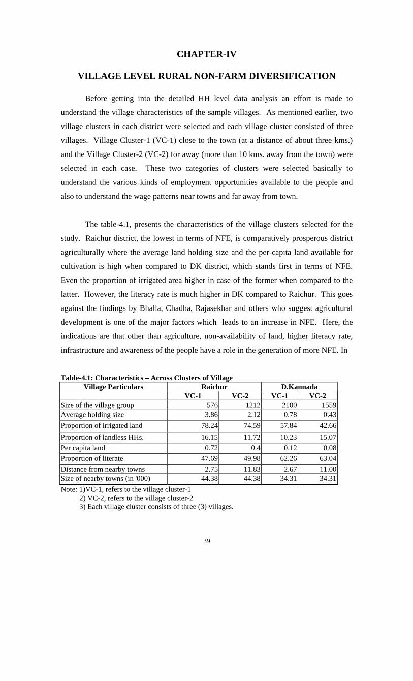
39

CHAPTER-IV

VILLAGE LEVEL RURAL NON-FARM DIVERSIFICATION

Before getting into the detailed HH level data analysis an effort is made to

understand the village characteristics of the sample villages. As mentioned earlier, two

village clusters in each district were selected and each village cluster consisted of three

villages. Village Cluster-1 (VC-1) close to the town (at a distance of about three kms.)

and the Village Cluster-2 (VC-2) for away (more than 10 kms. away from the town) were

selected in each case. These two categories of clusters were selected basically to

understand the various kinds of employment opportunities available to the people and

also to understand the wage patterns near towns and far away from town.

The table-4.1, presents the characteristics of the village clusters selected for the

study. Raichur district, the lowest in terms of NFE, is comparatively prosperous district

agriculturally where the average land holding size and the per-capita land available for

cultivation is high when compared to DK district, which stands first in terms of NFE.

Even the proportion of irrigated area higher in case of the former when compared to the

latter. However, the literacy rate is much higher in DK compared to Raichur. This goes

against the findings by Bhalla, Chadha, Rajasekhar and others who suggest agricultural

development is one of the major factors which leads to an increase in NFE. Here, the

indications are that other than agriculture, non-availability of land, higher literacy rate,

infrastructure and awareness of the people have a role in the generation of more NFE. In

Table-4.1: Characteristics – Across Clusters of Village Raichur D.Kannada Village Particulars

VC-1 VC-2 VC-1 VC-2 Size of the village group 576 1212 2100 1559Average holding size 3.86 2.12 0.78 0.43Proportion of irrigated land 78.24 74.59 57.84 42.66Proportion of landless HHs. 16.15 11.72 10.23 15.07Per capita land 0.72 0.4 0.12 0.08Proportion of literate 47.69 49.98 62.26 63.04Distance from nearby towns 2.75 11.83 2.67 11.00Size of nearby towns (in '000) 44.38 44.38 34.31 34.31Note: 1)VC-1, refers to the village cluster-1 2) VC-2, refers to the village cluster-2 3) Each village cluster consists of three (3) villages.

40

the absence of land for their livelihood people search for job. The Distress

Diversification hypothesis holds good in DK district in addition to the high literacy rate,

infrastructure and the awareness of the people. This has been explained in detail in the

following sections.

The above argument has been supported by the holding size of the farmers in the

sample villages. In the sample villages the number of marginal and small farmers is low

in the less developed district, Raichur, when compared to the developed district, DK.

Though there is a negative relationship between the land size class and the number of

holdings in DK, the decline in the number of holdings as the size class increases has been

high when compared to the Raichur district (Table-4.2). Table-4.2: No. of HHs Across Size Classes

Raichur D. Kannada Land Size Classes VC-1 VC-2 VC-1 VC-2

Marginal 150 587 1427 1121Small 170 253 330 126Semi Medium 153 212 128 66Medium 10 18 0 7Large 0 0 0 4Total 483 1070 1885 1324Note: Marginal Famrers=0.1 to 1 ha; Small Farmers=1.01 to 2.0 ha; Medium Famrers=2.01 to 5.00 ha; Large Farmers=5.01 ha and above

It is interesting to understand whether the villages, close to towns or the villages,

are far away from towns have more non-farm activities. The literature reveals that the

villages closer to towns have more NFE opportunities. To test this finding we have data

collected for the sample village clusters across various NFE activities. In Raichur district

the villages which are close to the town have more activities when compared to the

village clusters, far away from the town (Table 4.3). This is true for all the NFAs.

Whereas in DK, in the case of the traders and shopkeepers and services, we found that the

villages which were far away from the town performed better. Even for the other NFEAs

the difference is very narrow. This is mainly because of the awareness and higher

literacy levels of the people in these two districts. In DK the awareness and the literacy

rate are high and therefore, the people get into one activity or another. Second, the

villages in DK are spread across the main roads and the towns and villages are almost

clubbed, hence it is difficult to fix the boundaries of the villages. Therefore, one cannot

make differentiation between the villages near towns and far away from towns. Whereas

in Raichur the HHs are clustered and there is a clear-cut boundary for each village.

41

Table-4.3: No. of HHs Across Various Non-Farm Activities

Raichur D. Kannada Particulars VC-1 VC-2 VC-1 VC-2

Manufacturing and Processing 1.74 1.73 2.38 2.25 Construction 3.82 2.31 2.05 1.99 Traders and shop keepers 8.68 5.36 2.76 3.53 Transport 3.13 1.73 1.86 1.86 Services 5.21 4.62 2.00 2.50 The proportion of casual labourers across the industry categories have been

presented in Table-4.4. Agricultural labourers without land but engaged in allied

activities and agricultural labourers with land constitute the major portion of the casual

labourers in the study area. Of the two districts, Raichur seems to be the No. 1 in terms

of having more casual labourers. The third and the fifth places are taken by traders and

service sectors respectively.

Table-4.4: Proportion of the Casual Workers Across Industry Categories

Raichur D. Kannada Industrial Categories VC-1 VC-2 VC-1 VC-2

Agricultural labourers 16.15 11.72 10.24 15.07 Agri. Labourers with out land but with allied activity

42.53 29.04 20.24 35.28

Manufacturing, processing etc. 1.74 1.73 2.38 2.25 Construction 3.82 2.31 2.05 1.99 Trade 8.68 5.36 2.76 3.53 Transport 3.13 1.73 1.86 1.86 Services 5.21 4.62 2.00 2.50 An attempt is also made to understand the availability of infrastructure and

economic services in the sample villages. This has been presented in Table-4.5. By

understanding the characteristics of the districts, without any data one can say that

economic services are better in the DK villages when compared to Raichur. The

argument does hold good when we study the results which are presented in the table. The

table clearly reveals that of the 17 variables, four variables are not at all available in all

the villages. Of the 13 remaining variables, six variables are common in both the village

clusters. Of the seven variables, six variables seem to be high in DK district when

compared to the Raichur district. This shows that the DK villages are fully equipped with

infrastructure and economic services. Therefore, it is far ahead in terms of economic

development.

42

Table-4.5: Availability of Infrastructure and Economic Services in the Sample Villages

Infrastructure Facilities Raichur D.Kannada VC-1 VC-2 Total VC-1 VC-2 Total

Primary School 3 3 6 3 3 6Public School 0 2 2 3 1 4Primary Health Center 0 2 2 1 1 2Private Medical Practitioner 0 3 3 3 1 4Veterinary Dispensary 0 1 1 1 2 3Govt.training center 0 0 0 0 0 0Private Training center 0 0 0 0 0 0Khadi Village Industries 0 0 0 0 0 0Active ANGOs 3 3 6 3 3 6* Nearest Motorable Road 3 3 6 3 3 6Post Office 1 1 2 3 3 6Commercial Bank 0 0 0 2 0 2Co-operative Societies 1 0 1 2 1 3Existing Factories 1 0 1 2 0 2Farm Produce Storage 1 2 3 0 0 0Fair Price Shop 2 3 5 3 2 5Ag. Produce Market 0 0 0 0 0 0Note: Nearest motorable road is available in all the villages. Table-4.6 presents the livestock per ten households in the sample villages. DK

stands first in terms of owning local and crossbreed cows and also male buffaloes. For

drought animals like cattle, sheep and she-buffaloes, Raichur district dominates. In DK

he-buffaloes are used for cultivation purposes unlike bullocks which are used in Raichur.

Cows of various breeds are used for milching and therefore, dairying as NFA is high in

DK. Interestingly, the animal population has been higher in villages for away from towns

in both the districts.

Table-4.6: Distribution of Livestock Per Ten Households in the Sample Villages.

Various Animal Categories Raichur D. Kannada VC-1 VC-2 Avg. VC-1 VC-2 Avg.

Indigenous Cows 2.92 4.33 3.88 5.12 6.90 5.88Crossbreed Cows 0.07 0.05 0.06 0.20 0.30 0.24Buffaloes 7.10 17.72 14.30 1.67 0.37 1.12Draught Animals-Bullocks 1.56 1.96 1.83 0.83 0.64 0.75Male buffaloes 0.30 0.09 0.16 1.61 1.64 1.63Goats 5.76 5.82 5.80 0.85 0.46 0.69Sheep 3.40 3.67 3.59 0.00 0.15 0.06Others 0.00 0.17 0.11 0.78 0.00 0.45

The village level analysis clearly reveals that the distress diversification in

addition to the literacy rate, infrastructure and awareness of the people makes them

search for highly paid activity and are very important for NFE generation. These

characteristics we found to be higher in DK compared to Raichur district.

43

CHAPTER V

HOUSEHOLD LEVEL RURAL NON-FARM DIVERSIFICATION

As described in the methodology section, 120 sample HHs were selected to study

the pattern of employment in the sample districts. Of the sample, 60 each were drawn

from Raichur and DK districts. Of these, 30 each came from villages near towns and

from villages far away from towns (within three kms and above 10 kms respectively).

Before getting into the analysis of the patterns of RNFE, in the first section of the

chapter, we have given the socio-economic profile of the selected sample households in

the villages under study.

Section-I

Socio-Economic Profile of the Sample Households

Table 5.1 presents the distribution of sample HHs across various land size classes.

Though we have selected the HHs according to the industry categories, they fall into one

of these land size classes. The table clearly reveals that the number of landless, marginal

and small farmers is high and there are no medium and large farm categories in DK.

Even in Raichur district the number of landless, marginal and small farmers is high

compared to other categories of farmers. Though the total population of the DK district

is high the average family size seems to be low. And moreover, the family size of the

villages situated far away from towns is high when compared to those near towns (Table

5.2).

Table-5.1: Distribution of Sample HHs by Size of Operational Holdings

Raichur Dakshina Kannada Land size classes VC-1 VC-2 VC-1 VC-2

Landless 8 5 19 17 Marginal 11* 13 6 11 Small 6 8 5 2 Semi-Medium 3 4 0 0 Medium 2 0 0 0 Large 0 0 0 0 Total 30 30 30 30 Note: *One farmer in the marginal farm category has Leased out his land.

44

Table - 5.2: Category-wise Average Family Size of The Sample Households

Industry Categories Raichur Dakshina Kannada V1 V2 V1 V2

Small & Marginal 5.17 5.83 6.67 5.17 Manufacturing 6.50 7.57 5.13 4.17 Private Construction 5.67 5.33 3.33 7.00 Govt. aided construction 6.33 8.33 4.33 8.33 Whole sale Trading 7.33 5.00 6.67 5.67 Retail Trading 6.50 5.60 5.00 8.00 Transport 7.67 7.33 4.33 6.67 Total 6.33 6.47 5.23 6.23 The entire sample has houses of one or another. This means that 100 per cent of

the sample HHs owned residential houses. Therefore, we tried to see what kind of houses

they owned. We classified the houses into three categories based on the roof and the

material which used for the construction of the house. Pucca houses are made of RCC,

semi-pucca houses consists tiled roofs, mud walls and cement floors. Kutchcha houses

see made of thatched roofs, mud walls and cement floors. We found that most of the

sample HHs owned kutchha houses in Village Cluster-1 and semi-pucca houses in

Village Cluster-II of the Raichur district. However, in DK district most of the HHs

owned semi-pucca houses with tiled roofs. This clearly reveals that DK district is better

off when compared to Raichur district. Table 5.4 presents the number of animals per

family. The table reveals that Raichur is in a better position with respect to owning

animals when compared to DK district. The HHs engaged in government aided

construction, wholesale trading and retail trading and transport industry categories own

more animals per family in Raichur district. Table-5.3: Percentage of Self-Owned Houses Based on roof

Raichur D K V 1 V 2 V3 V4

Industry Categories

Pucca House

Semi- Pucca House

Kutchha House

Pucca House

Semi- Pucca House

Kutchha House

Pucca House

Semi- Pucca House

Kutchha

House

Pucca House

Semi- Pucca House

Kutchha

HouseSmall & Marginal 0.00 0.00 100 0.00 83.33 16.67 0.00 100.00 0.00 33.33 66.67 0.00

Manufacturing 0.00 62.50 37.50 14.29 28.57 57.14 37.50 62.50 0.00 16.67 83.33 0.00Private Construction

0.00 0.00 100.00 0.00 0.00 100.00 0.00 100.00 0.00 0.00 100.00 0.00

Govt. aided construction

33.33 0.00 66.67 33.33 66.67 0.00 66.67 33.33 0.00 33.33 66.67 0.00

Whole sale Trading

66.67 33.33 0.00 0.00 100.00 0.00 0.00 100.00 0.00 66.67 33.33 0.00

Retail Trading 0.00 75.00 25.00 0.00 80.00 20.00 0.00 100.00 0.00 33.33 66.67 0.00Transport 33.33 0.00 66.67 0.00 66.67 33.33 0.00 100.00 0.00 0.00 100.00 0.00Total 13.33 30.00 56.67 6.67 60.00 33.33 16.67 83.33 0.00 26.67 73.33 0.00*All the HHs have owned the houses.

45

Table-5.4:Average Number of Animals per Family

Raichur DK Name of Categories V1 V2 V3 V4

Small & Marginal 2.83 1.50 3.17 0.50Manufacturing 0.63 0.29 0.50 0.17Private Construction 1.33 0.33 0.67 1.33Govt. aided construction 4.67 10.33 0.00 1.33

Whole sale Trading 4.33 1.00 0.00 0.00Retail Trading 2.00 1.00 0.25 0.00Transport 3.67 0.33 0.67 0.00Total 2.40 1.73 0.93 0.40 Almost all the sample HHs owned beds, however, when it came to chairs and

tables the percentage came down considerably. The majority of the HHs owning chairs

and tables belong to the government-aided construction, whole sale trading and retail

trading industry categories in both the village clusters of Raichur district. In contrast, in

DK district, the majority of the HHs own all the three kinds of furniture, though the

percentage declines from one to another.

Table-5.5: Percentage of HHS having Various Kinds of Furniture

Raichur D K

V1 V2 V3 V4

Name of Category

Beds Chairs Tables Beds Chairs Tables Beds Chairs Tables Beds Chairs Tables Small & Marginal

100.00 33.33 0.00 100.00 83.33 16.67 100.00 83.33 100.00 100.00 100.00 66.67

Manufacturing 100.00 37.50 12.50 100.00 28.57 14.29 100.00 87.50 87.50 100.00 100.00 66.67Private Construction

100.00 0.00 0.00 100.00 33.33 0.00 100.00 33.33 33.33 100.00 100.00 33.33

Govt. aided construction

100.00 66.67 66.67 100.00 66.67 33.33 100.00 100.00 100.00 100.00 100.00 33.33

Whole sale Trading

100.00 100.00 66.67 100.00 100.00 33.33 100.00 100.00 100.00 100.00 100.00 33.33

Retail Trading 100.00 75.00 50.00 100.00 60.00 40.00 100.00 100.00 100.00 100.00 100.00 33.33Transport 100.00 33.33 33.33 100.00 66.67 33.33 100.00 33.33 33.33 100.00 100.00 66.67Totals 100.00 46.67 26.67 100.00 60.00 23.33 100.00 80.00 83.33 100.00 100.00 50.00 In Raichur district, the percentage of HHs owning durable goods like radio,

bicycles, television, motor bikes and other vehicles seems to be low when compared to

the DK district (Table 5.6). The HHs owning TV and motor bike belonged to

government aided construction and wholesale trading industry categories. In the case of

the HHs of the wholesale industry category almost every one owned TV in both the

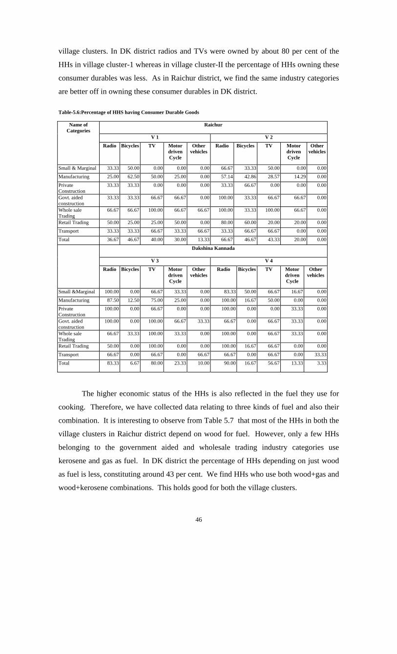
46

village clusters. In DK district radios and TVs were owned by about 80 per cent of the

HHs in village cluster-1 whereas in village cluster-II the percentage of HHs owning these

consumer durables was less. As in Raichur district, we find the same industry categories

are better off in owning these consumer durables in DK district.

Table-5.6:Percentage of HHS having Consumer Durable Goods

Name of Categories

Raichur

V 1 V 2

Radio Bicycles TV Motor driven Cycle

Other vehicles

Radio Bicycles TV Motor driven Cycle

Other vehicles

Small & Marginal 33.33 50.00 0.00 0.00 0.00 66.67 33.33 50.00 0.00 0.00

Manufacturing 25.00 62.50 50.00 25.00 0.00 57.14 42.86 28.57 14.29 0.00

Private Construction

33.33 33.33 0.00 0.00 0.00 33.33 66.67 0.00 0.00 0.00

Govt. aided construction

33.33 33.33 66.67 66.67 0.00 100.00 33.33 66.67 66.67 0.00

Whole sale Trading

66.67 66.67 100.00 66.67 66.67 100.00 33.33 100.00 66.67 0.00

Retail Trading 50.00 25.00 25.00 50.00 0.00 80.00 60.00 20.00 20.00 0.00

Transport 33.33 33.33 66.67 33.33 66.67 33.33 66.67 66.67 0.00 0.00

Total 36.67 46.67 40.00 30.00 13.33 66.67 46.67 43.33 20.00 0.00

Dakshina Kannada

V 3 V 4

Radio Bicycles TV Motor driven Cycle

Other vehicles

Radio Bicycles TV Motor driven Cycle

Other vehicles

Small &Marginal 100.00 0.00 66.67 33.33 0.00 83.33 50.00 66.67 16.67 0.00

Manufacturing 87.50 12.50 75.00 25.00 0.00 100.00 16.67 50.00 0.00 0.00

Private Construction

100.00 0.00 66.67 0.00 0.00 100.00 0.00 0.00 33.33 0.00

Govt. aided construction

100.00 0.00 100.00 66.67 33.33 66.67 0.00 66.67 33.33 0.00

Whole sale Trading

66.67 33.33 100.00 33.33 0.00 100.00 0.00 66.67 33.33 0.00

Retail Trading 50.00 0.00 100.00 0.00 0.00 100.00 16.67 66.67 0.00 0.00

Transport 66.67 0.00 66.67 0.00 66.67 66.67 0.00 66.67 0.00 33.33

Total 83.33 6.67 80.00 23.33 10.00 90.00 16.67 56.67 13.33 3.33

The higher economic status of the HHs is also reflected in the fuel they use for

cooking. Therefore, we have collected data relating to three kinds of fuel and also their

combination. It is interesting to observe from Table 5.7 that most of the HHs in both the

village clusters in Raichur district depend on wood for fuel. However, only a few HHs

belonging to the government aided and wholesale trading industry categories use

kerosene and gas as fuel. In DK district the percentage of HHs depending on just wood

as fuel is less, constituting around 43 per cent. We find HHs who use both wood+gas and

wood+kerosene combinations. This holds good for both the village clusters.

47

Table-5.7: Percentage of HHS with Availability of Technology for Cooking Purpose Raichur

V 1 V 2 Industry Categories

Wood Kerosene Gas Wood +Kerosene

Wood +Gas

Kerosene +Gas

Wood Kerosene Gas Wood +Kerosene

Wood +Gas

Kerosene + Gas

Small & Marginal 100.00 0.00 0.00 0.00 0.00 0.00 66.67 0.00 0.00 16.67 16.67 0.00Manufacturing 100.00 0.00 0.00 0.00 0.00 0.00 85.71 0.00 0.00 0.00 14.29 0.00Private Construction 100.00 0.00 0.00 0.00 0.00 0.00 100.00 0.00 0.00 0.00 0.00 0.00Govt. aided construction

33.33 0.00 0.00 33.33 33.33 0.00 66.67 0.00 0.00 0.00 33.33 0.00Whole sale Trading 0.00 33.33 0.00 33.33 33.33 0.00 33.33 0.00 33.33 0.00 33.33 0.00Retail Trading 75.00 0.00 0.00 25.00 0.00 0.00 80.00 0.00 0.00 0.00 20.00 0.00Transport 66.67 0.00 33.33 0.00 0.00 0.00 100.00 0.00 0.00 0.00 0.00 0.00Total 76.67 3.33 3.33 10.00 6.67 0.00 76.67 0.00 3.33 3.33 16.67 0.00

Industry Categories

Dakshina Kannada

V 3 V 4

Wood Kerosene Gas Wood + Kerosene

Wood +Gas

Kerosene + Gas

Wood Kerosene Gas Wood + Kerosene

Wood + Gas

Kerosene + Gas

Small & Marginal 66.66 0.00 0.00 0.00 33.33 0.00 0.00 0.00 0.00 50.00 50.00 0.00

Manufacturing 37.50 0.00 25.00 0.00 37.50 0.00 16.67 0.00 0.00 33.33 50.00 0.00

Private Construction 33.33 0.00 0.00 66.67 0.00 0.00 66.67 0.00 0.00 33.33 0.00 0.00

Govt. aided construction

33.33 0.00 66.67 0.00 0.00 0.00 33.33 0.00 0.00 0.00 66.67 0.00

Whole sale Trading 33.33 0.00 33.33 0.00 33.33 0.00 0.00 0.00 0.00 33.33 66.67 0.00

Retail Trading 25.00 0.00 50.00 0.00 25.00 0.00 0.00 0.00 16.67 16.67 50.00 16.67

Transport 66.67 0.00 0.00 0.00 33.33 0.00 0.00 0.00 0.00 66.67 33.33 0.00

Total 43.33 0.00 23.33 6.67 26.67 0.00 13.33 0.00 3.33 33.33 46.67 3.33

It is interesting to observe from Table 5.8, that around 50 per cent of the HHs in

the sample villages of Raichur district have bank accounts. Households involved in

private construction do not have bank accounts. More HHs belonging to the government

aided construction and wholesale trading industry categories have bank accounts. In DK

in village cluster-I almost all the HHs have bank accounts. Whereas in the village

cluster-II the figure is about 87 per cent. Therefore, one can say that in all respects DK’s

performance seems to be better when compared to Raichur district.

Table-5.8: Percentage of HHs Having Bank Account

Raichur Dakshina Kannada Industry Categories VC-1 VC-II VC-1 VC-II

Marginal and Small Farmers 50.00 50.00 100.00 100.00 Manufacturing 50.00 42.86 100.00 100.00 Private Construction 00 0.00 100.00 33.33 Govt. aided construction 66.67 66.67 100.00 66.67 Wholesale trading 66.67 100.00 100.00 66.67 Retail trading 50.00 40.00 100.00 100.00 Transport 66.67 66.67 100.00 100.00 Total 50.00 50.00 100.00 86.67

48

Section-II

Patrons of Rural Non-Farm Employment

In this section we have given the details regarding the patterns of RNFE in the

villages under study in both the districts. Table 5.9 presents the percentage distribution

of HHs by major sources of employment of the head of the households. We have tried to

give equal representation for all the industry categories. However, the representation is

little high in case of manufacturing, agriculture and allied activities. Weightage has been

given based on the concentration of the activity.

Table-5.9: Percentage Distribution of Households by Major Sources of Employment (Only Head of the HH).

Raichur Dakshina Kannada Industry Categories VC-1 VC-2 VC-1 VC-2

Agriculture 13.33 20.00 10.00 13.33Allied Activity 16.67 13.33 10.00 10.00Manufacturing, processing, services and repairs

20.00 16.67 26.67 20.00

Private construction 10.00 10.00 10.00 10.00Government aided construction 10.00 10.00 10.00 10.00Wholesale Traders 10.00 10.00 10.00 10.00Retail traders 10.00 10.00 13.33 20.00Services (transport, storage and Communication

10.00 10.00 10.00 10.00

Total No. HHs Total Per cent

30100

30 100 30 100 30 100

It is found that in case of all the sample HHs, there is more than one source of

income for the family (Table 5.10). The labourers who are involved in activities like

allied activities, regular employment in non-agriculture and the government construction

have a higher number of sources of income. Interestingly, villages situated far away from

the town have more sources of income when compared to the villages situated near

towns. Among the two districts, the number of sources of income are higher in DK

compared to Raichur district. This is mainly because of reasons, mentioned elsewhere

like education level, infrastructure, awareness and the inclination to do work.

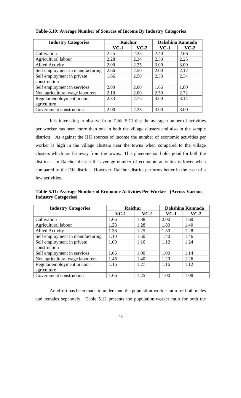
49

Table-5.10: Average Number of Sources of Income By Industry Categories

Raichur Dakshina Kannada Industry Categories VC-1 VC-2 VC-1 VC-2

Cultivation 2.25 2.33 2.40 2.66 Agricultural labour 2.28 2.34 2.30 2.25 Allied Activity 2.00 2.25 3.00 3.00 Self employment in manufacturing 2.66 2.50 2.00 2.12 Self employment in private construction

1.66 2.50 2.33 2.34

Self employment in services 2.00 2.00 1.66 1.80 Non agricultural wage labourers 2.10 2.00 2.50 2.72 Regular employment in non-agriculture

2.33 2.75 3.00 3.14

Government construction 2.00 2.33 3.00 3.00 It is interesting to observe from Table 5.11 that the average number of activities

per worker has been more than one in both the village clusters and also in the sample

districts. As against the HH sources of income the number of economic activities per

worker is high in the village clusters near the towns when compared to the village

clusters which are far away from the towns. This phenomenon holds good for both the

districts. In Raichur district the average number of economic activities is lower when

compared to the DK district. However, Raichur district performs better in the case of a

few activities.

Table-5.11: Average Number of Economic Activities Per Worker (Across Various Industry Categories)

Raichur Dakshina Kannada Industry Categories

VC-1 VC-2 VC-1 VC-2 Cultivation 1.66 1.38 2.00 1.60 Agricultural labour 1.23 1.28 1.80 1.40 Allied Activity 1.38 1.25 1.50 1.28 Self employment in manufacturing 1.10 1.50 1.40 1.46 Self employment in private construction

1.00 1.16 1.12 1.24

Self employment in services 1.66 1.00 1.00 1.14 Non agricultural wage labourers 1.46 1.40 1.20 1.26 Regular employment in non-agriculture

1.16 1.27 1.16 1.12

Government construction 1.66 1.25 1.00 1.00 An effort has been made to understand the population-worker ratio for both males

and females separately. Table 5.12 presents the population-worker ratio for both the

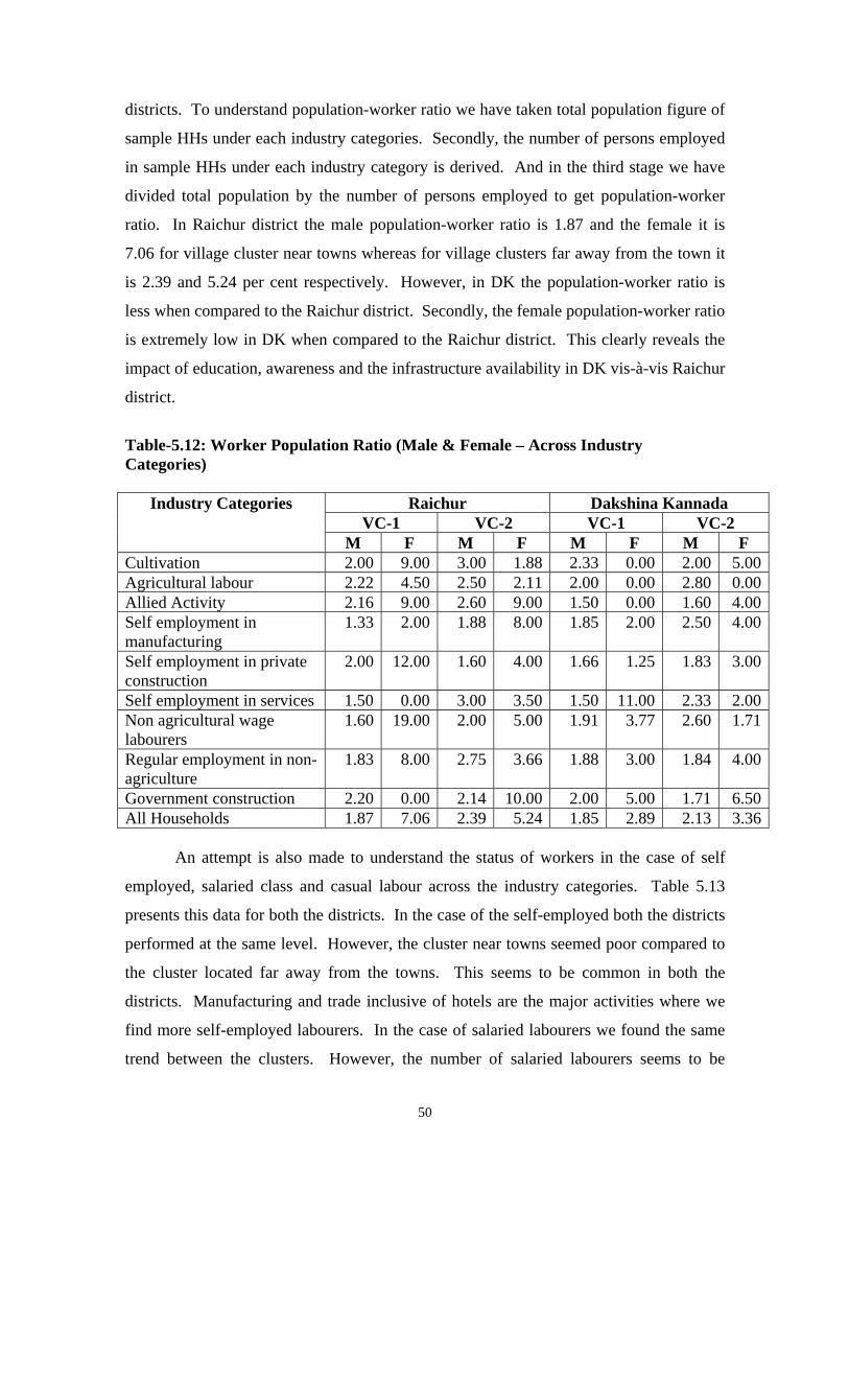
50

districts. To understand population-worker ratio we have taken total population figure of

sample HHs under each industry categories. Secondly, the number of persons employed

in sample HHs under each industry category is derived. And in the third stage we have

divided total population by the number of persons employed to get population-worker

ratio. In Raichur district the male population-worker ratio is 1.87 and the female it is

7.06 for village cluster near towns whereas for village clusters far away from the town it

is 2.39 and 5.24 per cent respectively. However, in DK the population-worker ratio is

less when compared to the Raichur district. Secondly, the female population-worker ratio

is extremely low in DK when compared to the Raichur district. This clearly reveals the

impact of education, awareness and the infrastructure availability in DK vis-à-vis Raichur

district.

Table-5.12: Worker Population Ratio (Male & Female – Across Industry Categories)

Raichur Dakshina Kannada VC-1 VC-2 VC-1 VC-2

Industry Categories

M F M F M F M F Cultivation 2.00 9.00 3.00 1.88 2.33 0.00 2.00 5.00Agricultural labour 2.22 4.50 2.50 2.11 2.00 0.00 2.80 0.00Allied Activity 2.16 9.00 2.60 9.00 1.50 0.00 1.60 4.00Self employment in manufacturing

1.33 2.00 1.88 8.00 1.85 2.00 2.50 4.00

Self employment in private construction

2.00 12.00 1.60 4.00 1.66 1.25 1.83 3.00

Self employment in services 1.50 0.00 3.00 3.50 1.50 11.00 2.33 2.00Non agricultural wage labourers

1.60 19.00 2.00 5.00 1.91 3.77 2.60 1.71

Regular employment in non-agriculture

1.83 8.00 2.75 3.66 1.88 3.00 1.84 4.00

Government construction 2.20 0.00 2.14 10.00 2.00 5.00 1.71 6.50All Households 1.87 7.06 2.39 5.24 1.85 2.89 2.13 3.36 An attempt is also made to understand the status of workers in the case of self

employed, salaried class and casual labour across the industry categories. Table 5.13

presents this data for both the districts. In the case of the self-employed both the districts

performed at the same level. However, the cluster near towns seemed poor compared to

the cluster located far away from the towns. This seems to be common in both the

districts. Manufacturing and trade inclusive of hotels are the major activities where we

find more self-employed labourers. In the case of salaried labourers we found the same

trend between the clusters. However, the number of salaried labourers seems to be

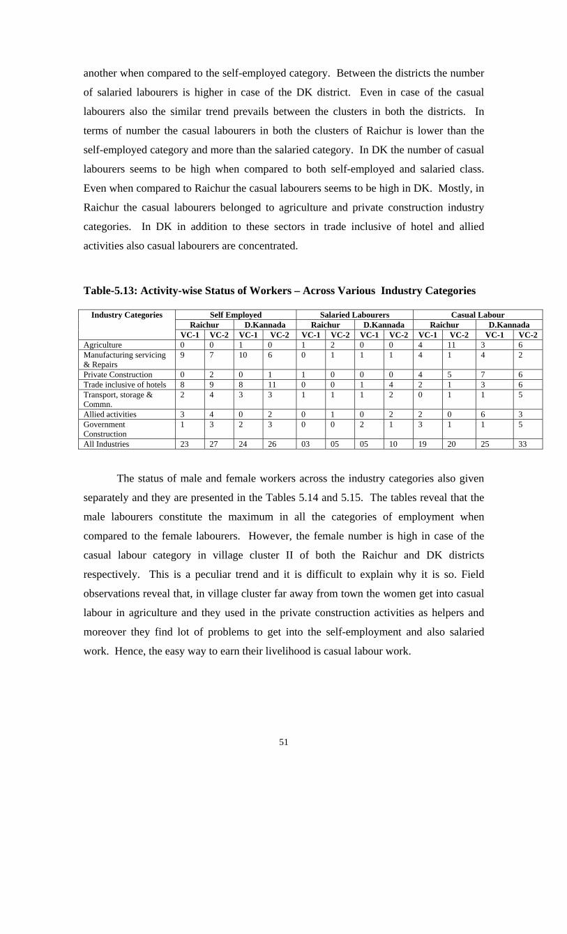
51

another when compared to the self-employed category. Between the districts the number

of salaried labourers is higher in case of the DK district. Even in case of the casual

labourers also the similar trend prevails between the clusters in both the districts. In

terms of number the casual labourers in both the clusters of Raichur is lower than the

self-employed category and more than the salaried category. In DK the number of casual

labourers seems to be high when compared to both self-employed and salaried class.

Even when compared to Raichur the casual labourers seems to be high in DK. Mostly, in

Raichur the casual labourers belonged to agriculture and private construction industry

categories. In DK in addition to these sectors in trade inclusive of hotel and allied

activities also casual labourers are concentrated.

Table-5.13: Activity-wise Status of Workers – Across Various Industry Categories

Self Employed Salaried Labourers Casual Labour Raichur D.Kannada Raichur D.Kannada Raichur D.Kannada

Industry Categories

VC-1 VC-2 VC-1 VC-2 VC-1 VC-2 VC-1 VC-2 VC-1 VC-2 VC-1 VC-2 Agriculture 0 0 1 0 1 2 0 0 4 11 3 6 Manufacturing servicing & Repairs

9 7 10 6 0 1 1 1 4 1 4 2

Private Construction 0 2 0 1 1 0 0 0 4 5 7 6 Trade inclusive of hotels 8 9 8 11 0 0 1 4 2 1 3 6 Transport, storage & Commn.

2 4 3 3 1 1 1 2 0 1 1 5

Allied activities 3 4 0 2 0 1 0 2 2 0 6 3 Government Construction

1 3 2 3 0 0 2 1 3 1 1 5

All Industries 23 27 24 26 03 05 05 10 19 20 25 33 The status of male and female workers across the industry categories also given

separately and they are presented in the Tables 5.14 and 5.15. The tables reveal that the

male labourers constitute the maximum in all the categories of employment when

compared to the female labourers. However, the female number is high in case of the

casual labour category in village cluster II of both the Raichur and DK districts

respectively. This is a peculiar trend and it is difficult to explain why it is so. Field

observations reveal that, in village cluster far away from town the women get into casual

labour in agriculture and they used in the private construction activities as helpers and

moreover they find lot of problems to get into the self-employment and also salaried

work. Hence, the easy way to earn their livelihood is casual labour work.

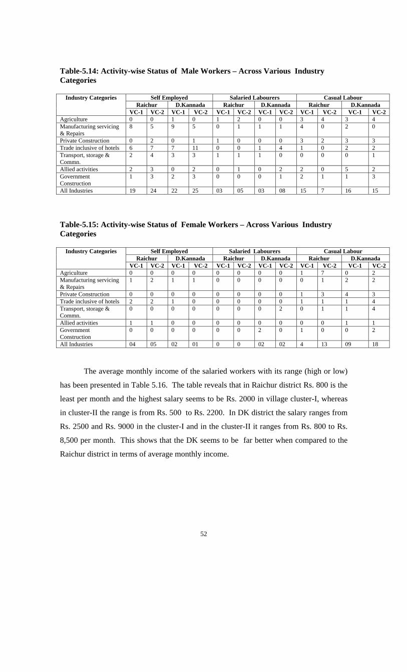
52

Table-5.14: Activity-wise Status of Male Workers – Across Various Industry Categories

Self Employed Salaried Labourers Casual Labour Raichur D.Kannada Raichur D.Kannada Raichur D.Kannada

Industry Categories

VC-1 VC-2 VC-1 VC-2 VC-1 VC-2 VC-1 VC-2 VC-1 VC-2 VC-1 VC-2 Agriculture 0 0 1 0 1 2 0 0 3 4 3 4 Manufacturing servicing & Repairs

8 5 9 5 0 1 1 1 4 0 2 0

Private Construction 0 2 0 1 1 0 0 0 3 2 3 3 Trade inclusive of hotels 6 7 7 11 0 0 1 4 1 0 2 2 Transport, storage & Commn.

2 4 3 3 1 1 1 0 0 0 0 1

Allied activities 2 3 0 2 0 1 0 2 2 0 5 2 Government Construction

1 3 2 3 0 0 0 1 2 1 1 3

All Industries 19 24 22 25 03 05 03 08 15 7 16 15 Table-5.15: Activity-wise Status of Female Workers – Across Various Industry Categories

Self Employed Salaried Labourers Casual Labour Raichur D.Kannada Raichur D.Kannada Raichur D.Kannada

Industry Categories

VC-1 VC-2 VC-1 VC-2 VC-1 VC-2 VC-1 VC-2 VC-1 VC-2 VC-1 VC-2 Agriculture 0 0 0 0 0 0 0 0 1 7 0 2 Manufacturing servicing & Repairs

1 2 1 1 0 0 0 0 0 1 2 2

Private Construction 0 0 0 0 0 0 0 0 1 3 4 3 Trade inclusive of hotels 2 2 1 0 0 0 0 0 1 1 1 4 Transport, storage & Commn.

0 0 0 0 0 0 0 2 0 1 1 4

Allied activities 1 1 0 0 0 0 0 0 0 0 1 1 Government Construction

0 0 0 0 0 0 2 0 1 0 0 2

All Industries 04 05 02 01 0 0 02 02 4 13 09 18 The average monthly income of the salaried workers with its range (high or low)

has been presented in Table 5.16. The table reveals that in Raichur district Rs. 800 is the

least per month and the highest salary seems to be Rs. 2000 in village cluster-I, whereas

in cluster-II the range is from Rs. 500 to Rs. 2200. In DK district the salary ranges from

Rs. 2500 and Rs. 9000 in the cluster-I and in the cluster-II it ranges from Rs. 800 to Rs.

8,500 per month. This shows that the DK seems to be far better when compared to the

Raichur district in terms of average monthly income.

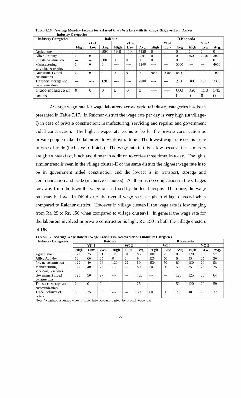
53

Table-5.16: Average Monthly Income for Salaried Class Workers with its Range (High or Low) Across Industry Categories

Raichur D.Kannada VC-1 VC-2 VC-1 VC-2

Industry Categories

High Low Avg. High Low Avg. High Low Avg. High Low Avg. Agriculture --- ---- 2000 1200 1100 1150 0 0 0 0 0 0 Allied Activity 0 0 0 ---- ---- 500 0 0 0 3500 2500 3000 Private construction --- --- 800 0 0 0 0 0 0 0 0 0 Manufacturing, servicing & repairs

0 0 0 ---- ---- 1200 ---- ---- 3000 ---- ---- 4000

Government aided construction

0 0 0 0 0 0 9000 4000 6500 ---- ---- 1000

Transport, storage and communication

--- ---- 1200 ---- ---- 2200 ---- ---- 2500 5800 800 3300

Trade inclusive of hotels

0 0 0 0 0 0 ---- ---- 6000

8500

1500

5450

Average wage rate for wage labourers across various industry categories has been

presented in Table 5.17. In Raichur district the wage rate per day is very high (in village-

I) in case of private construction; manufacturing, servicing and repairs; and government

aided construction. The highest wage rate seems to be for the private construction as

private people make the labourers to work extra time. The lowest wage rate seems to be

in case of trade (inclusive of hotels). The wage rate in this is low because the labourers

are given breakfast, lunch and dinner in addition to coffee three times in a day. Though a

similar trend is seen in the village cluster-II of the same district the highest wage rate is to

be in government aided construction and the lowest is in transport, storage and

communication and trade (inclusive of hotels). As there is no competition in the villages

far away from the town the wage rate is fixed by the local people. Therefore, the wage

rate may be low. In DK district the overall wage rate is high in village cluster-I when

compared to Raichur district. However in village cluster-II the wage rate is low ranging

from Rs. 25 to Rs. 150 when compared to village cluster-1. In general the wage rate for

the labourers involved in private construction is high, Rs. 150 in both the village clusters

of DK. Table-5.17: Average Wage Rate for Wage Labourers- Across Various Industry Categories

Raichur D.Kannada VC-1 VC-2 VC-1 VC-2

Industry Categories

High Low Avg. High Low Avg. High Low Avg. High Low Avg. Agriculture 120 25 61 120 30 55 100 75 83 120 20 57 Allied Activity 70 60 65 0 0 0 120 50 84 35 25 30 Private construction 120 40 98 120 25 50 150 50 89 150 20 58 Manufacturing, servicing & repairs

120 40 73 --- --- 50 50 50 50 25 25 25

Government aided construction

120 50 97 --- --- 120 --- --- 120 125 25 64

Transport, storage and communication

0 0 0 --- --- 25 --- --- 50 120 20 59

Trade inclusive of hotels

50 25 38 --- --- 30 80 50 70 40 25 32

Note: Weighted Average value is taken into account to give the overall wage rate.

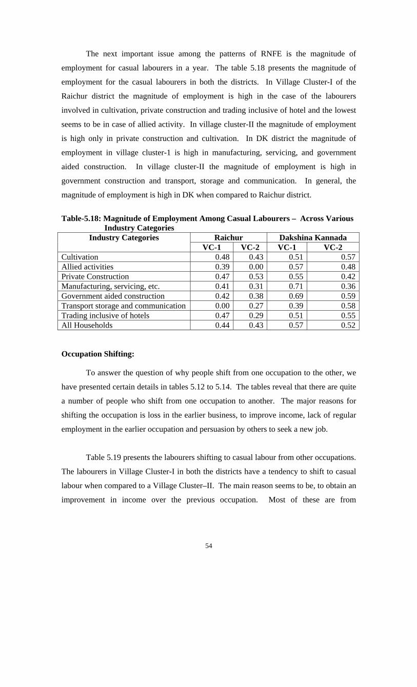
54

The next important issue among the patterns of RNFE is the magnitude of

employment for casual labourers in a year. The table 5.18 presents the magnitude of

employment for the casual labourers in both the districts. In Village Cluster-I of the

Raichur district the magnitude of employment is high in the case of the labourers

involved in cultivation, private construction and trading inclusive of hotel and the lowest

seems to be in case of allied activity. In village cluster-II the magnitude of employment

is high only in private construction and cultivation. In DK district the magnitude of

employment in village cluster-1 is high in manufacturing, servicing, and government

aided construction. In village cluster-II the magnitude of employment is high in

government construction and transport, storage and communication. In general, the

magnitude of employment is high in DK when compared to Raichur district.

Table-5.18: Magnitude of Employment Among Casual Labourers – Across Various

Industry Categories Raichur Dakshina Kannada Industry Categories

VC-1 VC-2 VC-1 VC-2 Cultivation 0.48 0.43 0.51 0.57Allied activities 0.39 0.00 0.57 0.48Private Construction 0.47 0.53 0.55 0.42Manufacturing, servicing, etc. 0.41 0.31 0.71 0.36Government aided construction 0.42 0.38 0.69 0.59Transport storage and communication 0.00 0.27 0.39 0.58Trading inclusive of hotels 0.47 0.29 0.51 0.55All Households 0.44 0.43 0.57 0.52 Occupation Shifting: To answer the question of why people shift from one occupation to the other, we

have presented certain details in tables 5.12 to 5.14. The tables reveal that there are quite

a number of people who shift from one occupation to another. The major reasons for

shifting the occupation is loss in the earlier business, to improve income, lack of regular

employment in the earlier occupation and persuasion by others to seek a new job.

Table 5.19 presents the labourers shifting to casual labour from other occupations.

The labourers in Village Cluster-I in both the districts have a tendency to shift to casual

labour when compared to a Village Cluster–II. The main reason seems to be, to obtain an

improvement in income over the previous occupation. Most of these are from

55

agriculture, allied activities and government construction. Proximity to town where they

get more return may be the reason for this.

Table-5.19:Frequency of Labourers Shifting to Casual Labour – According to Reasons

Raichur Dakshina Kannada District VC-1 VC-2 VC-1 VC-2

Industry Categories

No I II III IV No I II III IV No I II III IV No I II III IV Agriculture 2 2 0 0 0 2 0 1 1 0 3 0 3 0 0 2 1 1 0 0 Allied activity 2 0 1 1 0 0 0 0 0 0 2 0 2 0 0 1 0 1 0 0 Manufacturing servicing & Repairs

1 0 1 0 0 0 0 0 0 0 1 0 0 1 0 0 0 0 0 0

Transport, storage & Comcn.

0 0 0 0 0 0 0 0 0 0 0 0 0 0 0 0 0 0 0 0

Private Construction

1 1 0 0 0 1 0 1 0 0 2 0 2 0 0 1 0 0 1 0

Government aided construction.

2 0 2 0 0 0 0 0 0 0 1 0 1 0 0 0 0 0 0 0

Wholesale trading 0 0 0 0 0 0 0 0 0 0 1 0 0 1 0 0 0 0 0 0 Retail trading 0 0 0 0 0 0 0 0 0 0 0 0 0 0 0 0 0 0 0 0 All Industry Categories

8 3 4 1 0 3 0 2 1 0 10 8 2 0 4 1 2 1 0

Note: 1) I= Loss in the earlier business, II = To have improvement over income, III = Lack of regular employment, IV = Motivated by others.

The table 5.20 presents the labourers shifting to salaried employment from various

other occupations. The labourers shifting to salaried employment is very minimum as it

is not easy to get salaried employment. However, village cluster-II in Raichur district

seems to be better in terms of shifting to salaried employment. The reason they have

given for the change is the lack of regular employment in the earlier occupations like

agriculture, allied activities and manufacturing, servicing and repairs.

Table-5.20: Frequency of Labourers Shifting to Salaried Employment – According to Reasons

Raichur Dakshina Kannada District VC-1 VC-2 VC-1 VC-2

Industry Categories

No I II III IV No I II III IV No I II III IV No I II III IV Agriculture 1 0 0 1 0 2 0 0 2 0 0 0 0 0 0 0 0 0 0 0 Allied activity 0 0 0 0 0 1 0 0 1 0 1 0 1 0 0 1 0 1 0 0 Manufacturing servicing & Repairs

0 0 0 0 0 1 0 0 1 0 0 0 0 0 0 0 0 0 0 0

Transport, storage & Comcn.

0 0 0 0 0 0 0 0 0 0 0 0 0 0 0 0 0 0 0 0

Private Construction

0 0 0 0 0 0 0 0 0 0 0 0 0 0 0 0 0 0 0 0

Government aided construction.

0 0 0 0 0 0 0 0 0 0 0 0 0 0 0 0 0 0 0 0

Wholesale trading 0 0 0 0 0 0 0 0 0 0 0 0 0 0 0 0 0 0 0 0 Retail trading 0 0 0 0 0 0 0 0 0 0 1 0 0 1 0 0 0 0 0 0 All Industry Categories

1 0 0 1 0 4 0 0 4 0 2 0 1 1 0 1 0 1 0 0

Note: 1) I= Loss in the earlier business, II = To have improvement over income, III = Lack of regular employment, IV = Motivated by others.

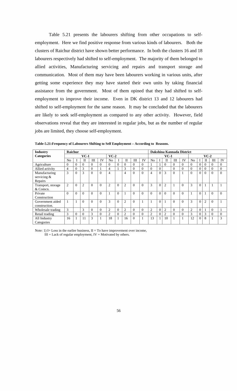
56

Table 5.21 presents the labourers shifting from other occupations to self-

employment. Here we find positive response from various kinds of labourers. Both the

clusters of Raichur district have shown better performance. In both the clusters 16 and 18

labourers respectively had shifted to self-employment. The majority of them belonged to

allied activities, Manufacturing servicing and repairs and transport storage and

communication. Most of them may have been labourers working in various units, after

getting some experience they may have started their own units by taking financial

assistance from the government. Most of them opined that they had shifted to self-

employment to improve their income. Even in DK district 13 and 12 labourers had

shifted to self-employment for the same reason. It may be concluded that the labourers

are likely to seek self-employment as compared to any other activity. However, field

observations reveal that they are interested in regular jobs, but as the number of regular

jobs are limited, they choose self-employment.

Table-5.21:Frequency of Labourers Shifting to Self Employment – According to Reasons.

Raichur Dakshina Kannada District VC-1 VC-2 VC-1 VC-2

Industry Categories

No I II III IV No I II III IV No I II III IV No I II III IV Agriculture 0 0 0 0 0 0 0 0 0 0 1 1 0 0 0 0 0 0 0 0 Allied activity 4 0 3 0 1 4 1 3 0 0 0 0 0 0 0 0 0 0 0 Manufacturing servicing & Repairs

3 0 3 0 0 4 4 0 0 4 0 3 0 1 0 0 0 0 0

Transport, storage & Comcn.

2 0 2 0 0 2 0 2 0 0 3 0 2 1 0 3 0 1 1 1

Private Construction

0 0 0 0 0 1 0 1 0 0 0 0 0 0 0 1 0 1 0 0

Government aided construction.

1 1 0 0 0 3 0 2 0 1 1 0 1 0 0 3 0 2 0 1

Wholesale trading 3 3 0 0 2 0 2 0 0 2 0 2 0 0 2 0 1 0 1 Retail trading 3 0 0 3 0 2 0 2 0 0 2 0 2 0 0 3 0 3 0 0 All Industry Categories

16 1 11 3 1 18 1 16 0 1 13 1 10 1 1 12 0 8 1 3

Note: 1) I= Loss in the earlier business, II = To have improvement over income, III = Lack of regular employment, IV = Motivated by others.

57

CHAPTER VI

STATUS OF ENTERPRISES IN THE STATE WITH SPECIAL

REFERENCE TO THE PROCESSING SECTOR & EMPLOYMENT GENERATION ACROSS THREE INDUSTRIAL CATEGORIES

As mentioned elsewhere, the data for this particular section is not available at the

district level. Therefore, we have concentrated on a state level analysis. In this chapter

we have tried to collect data from 1989-90 to 1997-98 from the annual survey of

industries. In the first section of the analysis we have tried to see the performance of

various Agro-Processing Industry Units (APIUs) within the sector. In the second section

we have tried to assess the performance of agro-processing units with reference to the

total industry sector in the state. And in the third section we have highlighted

employment generation across three industrial categories, viz., OAMEs, NDMEs and

DMEs based on the Economic Census and NSSO reports. It is hoped that this will give

the performance of the APIUs within the sector, which are most probably concentrated in

the rural areas of Karnataka and their share in the total industry sector, and show

employment generation across various industry categories.

Section-1

Performance of APIUs with in the Sector: Growth of the Units

The APIUs like food products; beverages and tobacco; cotton textiles; wool silk

and manmade fiber; jute and vegetable fibre; textile products; wood and its products;

paper and leather are most important. The performance of each unit has been presented

in Table 6.1. The performance of these has been equated to 100 and studied one by one

over a period of nine years. Compound growth rate has been worked out to study

accuracy in terms of performance. In Table 6.1 we have shown the growth of the number

of units in terms of percentage. Among the units food products play a prominent role.

However, from about 40 per cent in 1989-90, it has declined slowly to 36.69 per cent by

1997-98 - decline in the growth rate by 1.23 per cent per annum. The second, third and

fourth places, in terms of share, is held by cotton textiles, wood and paper industries,

however their growth rate has been negative. Except beverages, which is showing a

58

growth rate of about 2 per cent per annum and for which the percentage share is also

high, all the other units have been showing negative growth. In the case of the leather

industry, though the percentage share is low, the growth rate is high. The data reveals

that over a period of about nine years, the APIUs have declined in number. Discussions

with officials and entrepreneurs revealed three reasons for the poor performance. Firstly,

they say that the rainfall is uncertain and that production in general has come down.

Second, they say that liberalisation has lead to import of food products like oil and other

goods, which lead to unit closure, but there is no initiative to start the units though they

are providing capital investment subsidy in the range of 15 to 35 per cent. Third, which

is most important, is the government is not able to provide required infrastructure

specially, market support, electricity and proper road facility.

Table-6.1: Growth of the Units within the APIUs (Fig in %)

Year Food products

Beverages,Tobacco

Cotton textiles

Wool, Silk & Man-made fiber

Jute & Vegetable

fiber

Textile products

Wood Paper Leather Total

1989-90 40.04 4.83 18.38 6.53 0.26 6.90 10.96 10.66 1.44 1001990-91 39.08 6.13 17.43 6.99 0.14 8.71 9.25 10.54 1.72 1001991-92 39.61 5.81 17.71 6.49 0.18 9.49 8.08 10.61 2.02 1001992-93 39.61 5.81 17.71 6.49 0.18 9.49 8.08 10.61 2.02 1001993-94 39.23 6.02 16.22 5.53 0.21 12.63 8.23 9.48 2.46 1001994-95 35.81 7.02 15.78 5.72 0.21 15.75 6.91 9.82 2.98 1001995-96 35.58 5.51 14.50 5.71 0.20 17.47 6.65 10.96 3.41 1001996-97 38.05 6.19 14.79 5.65 0.21 17.28 6.86 7.57 3.38 1001997-98 36.69 6.33 14.53 5.20 0.16 18.48 5.33 10.98 2.29 100GR in % -1.23 2.005 -3.19 -3.17 -0.53 13.74 -6.96 -1.47 9.276 -- Source: Various Issues of Annual Survey of Industries: CSO, GOI. The Status of Employment:

It is interesting to observe from the table 6.2 that in the APIUs the growth rate is

negative in all the Units except textile products. It is highly difficult to correlate the

growth of the number of units and the employment generation in beverages and leather

industry units. Here, the growth has been positive in terms of number of units but the

employment growth rate has been negative. One reason could be that in these units

improved technology has been introduced. In contrast in the textile industry units there

is a scope for manual labour as it is more labour intensive. Therefore, the employment

generation is high in this industry sector. The same holds good in case of the wool, silk

and man-made fiber industry units where the growth rate of employment has been

59

positive. However, the concentration of employment can be seen in case of food

products, paper, cotton textile, beverages and wool-silk-man made fiber industry units.

Table-6.2: Growth of Employment with in APIUs (Fig in %)

Year Food products

Beverages,Tobacco

Cotton textiles

Wool, Silk & Man-made fibre

Jute & Vegetable

fibre

Textile products

Wood Paper Leather Total

1989-90 34.76 6.95 24.65 3.94 0.21 11.37 4.09 12.19 1.84 1001990-91 32.00 7.01 21.51 4.74 0.13 15.09 3.39 13.46 2.67 1001991-92 31.52 6.80 21.02 5.48 0.14 17.70 1.91 12.80 2.63 1001992-93 31.52 6.80 21.02 5.48 0.14 17.70 1.91 12.80 2.63 1001993-94 28.23 7.34 19.53 4.84 0.14 25.05 3.20 8.54 3.12 1001994-95 26.29 7.05 15.23 4.34 0.09 31.69 2.27 9.02 4.01 1001995-96 25.89 5.49 14.39 5.04 0.11 34.87 1.51 9.00 3.70 1001996-97 26.84 6.74 12.20 3.81 0.09 36.59 1.36 8.03 4.36 1001997-98 23.10 6.41 12.54 5.54 0.06 36.95 0.98 9.07 5.35 100GR in % -4.46 -1.38 -8.74 0.525 -11.5 16.79 -13.6 -6.12 12.1 -- Source: As in table 6.1. Capital Investment in the APIUs:

The growth rate of capital investment gives the explanation for the slow or low or

negative employment growth rate in so many sectors with-in the APIUs. The APIUs like

wool, silk and man made fibre; jute and vegetable fiber, textile products; paper and wood

industries show positive growth rate in capital investment (Table 6.3). This is mainly

because, in these units the capital-intensive techniques are being used. Therefore, the

employment generation is low though the capital investment is high.

Table-6.3: Growth of Capital Investment within the APIUs (Fig. In %)

Year Food products

Beverages,Tobacco

Cotton textiles

Wool, Silk & Man-made fibre

Jute & Vegetable

fibre

Textile products

Wood Paper Leather Total

1989-90 53.18 7.95 11.70 2.45 0.01 4.76 2.63 14.10 3.23 1001990-91 48.49 9.11 11.85 5.04 0.01 5.88 1.73 13.77 4.11 1001991-92 48.53 9.25 13.43 4.94 0.01 6.94 0.72 13.44 2.73 1001992-93 47.43 9.13 12.71 5.27 0.03 8.77 1.73 12.70 2.22 1001993-94 49.97 9.23 11.43 5.39 0.01 10.78 1.26 8.09 3.85 1001994-95 39.08 11.50 13.78 4.08 0.03 14.69 1.33 12.02 3.51 1001995-96 41.27 6.10 12.53 6.64 0.02 13.90 1.27 12.94 5.33 1001996-97 41.61 8.59 7.16 9.47 0.02 10.47 1.02 16.40 5.26 1001997-98 32.36 8.56 8.11 12.15 0.00 12.16 0.51 21.99 4.16 100GR in % -4.82 -0.8 -4.93 15.48 4.5 13.1 -11.5 3.68 6.095 -- Source: As in table 6.1

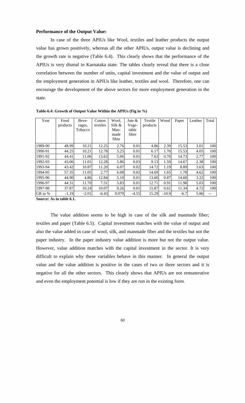
60

Performance of the Output Value:

In case of the three APIUs like Wool, textiles and leather products the output

value has grown positively, whereas all the other APIUs, output value is declining and

the growth rate is negative (Table 6.4). This clearly shows that the performance of the

APIUs is very dismal in Karnataka state. The tables clearly reveal that there is a close

correlation between the number of units, capital investment and the value of output and

the employment generation in APIUs like leather, textiles and wool. Therefore, one can

encourage the development of the above sectors for more employment generation in the

state.

Table-6.4: Growth of Output Value Within the APIUs (Fig in %)

Year Food products

Beve-rages,

Tobacco

Cotton textiles

Wool, Silk & Man-made fibre

Jute & Vege-table fibre

Textile products

Wood Paper Leather Total

1989-90 48.99 10.21 12.25 2.76 0.01 4.86 2.39 15.53 3.01 1001990-91 44.25 10.21 12.78 5.25 0.01 6.17 1.76 15.53 4.05 1001991-92 44.41 11.06 13.63 5.06 0.01 7.63 0.70 14.73 2.77 1001992-93 43.06 11.01 12.28 5.86 0.03 9.13 1.59 14.67 2.38 1001993-94 43.42 10.87 11.20 6.07 0.02 14.72 1.19 8.89 3.63 1001994-95 57.35 11.05 2.77 6.08 0.02 14.69 1.65 1.78 4.62 1001995-96 44.90 4.86 12.84 5.10 0.01 13.60 0.87 14.60 3.22 1001996-97 44.31 11.70 7.51 5.83 0.01 12.71 0.91 11.98 5.03 1001997-98 37.87 10.24 10.07 9.26 0.01 15.87 0.61 11.34 4.72 100GR in % -1.19 -2.01 -6.43 9.079 -4.55 15.29 -10.9 -6.7 5.86 -- Source: As in table 6.1. The value addition seems to be high in case of the silk and manmade fiber;

textiles and paper (Table 6.5). Capital investment matches with the value of output and

also the value added in case of wool, silk, and manmade fiber and the textiles but not the

paper industry. In the paper industry value addition is more but not the output value.

However, value addition matches with the capital investment in the sector. It is very

difficult to explain why these variables behave in this manner. In general the output

value and the value addition is positive in the cases of two or three sectors and it is

negative for all the other sectors. This clearly shows that APIUs are not remunerative

and even the employment potential is low if they are run in the existing form.

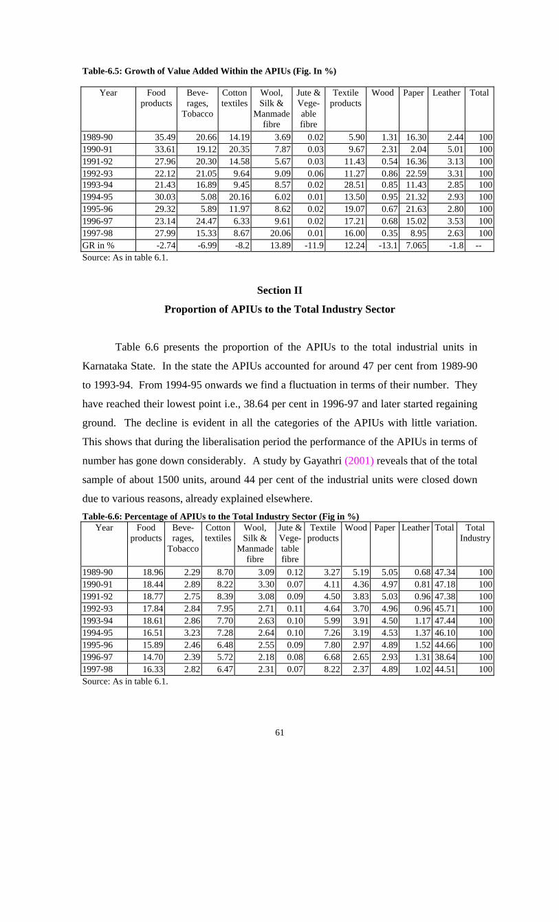
61

Table-6.5: Growth of Value Added Within the APIUs (Fig. In %)

Year Food products

Beve-rages,

Tobacco

Cotton textiles

Wool, Silk &

Manmade fibre

Jute & Vege-able fibre

Textile products

Wood Paper Leather Total

1989-90 35.49 20.66 14.19 3.69 0.02 5.90 1.31 16.30 2.44 1001990-91 33.61 19.12 20.35 7.87 0.03 9.67 2.31 2.04 5.01 1001991-92 27.96 20.30 14.58 5.67 0.03 11.43 0.54 16.36 3.13 1001992-93 22.12 21.05 9.64 9.09 0.06 11.27 0.86 22.59 3.31 1001993-94 21.43 16.89 9.45 8.57 0.02 28.51 0.85 11.43 2.85 1001994-95 30.03 5.08 20.16 6.02 0.01 13.50 0.95 21.32 2.93 1001995-96 29.32 5.89 11.97 8.62 0.02 19.07 0.67 21.63 2.80 1001996-97 23.14 24.47 6.33 9.61 0.02 17.21 0.68 15.02 3.53 1001997-98 27.99 15.33 8.67 20.06 0.01 16.00 0.35 8.95 2.63 100GR in % -2.74 -6.99 -8.2 13.89 -11.9 12.24 -13.1 7.065 -1.8 -- Source: As in table 6.1.

Section II

Proportion of APIUs to the Total Industry Sector

Table 6.6 presents the proportion of the APIUs to the total industrial units in

Karnataka State. In the state the APIUs accounted for around 47 per cent from 1989-90

to 1993-94. From 1994-95 onwards we find a fluctuation in terms of their number. They

have reached their lowest point i.e., 38.64 per cent in 1996-97 and later started regaining

ground. The decline is evident in all the categories of the APIUs with little variation.

This shows that during the liberalisation period the performance of the APIUs in terms of

number has gone down considerably. A study by Gayathri (2001) reveals that of the total

sample of about 1500 units, around 44 per cent of the industrial units were closed down

due to various reasons, already explained elsewhere. Table-6.6: Percentage of APIUs to the Total Industry Sector (Fig in %)

Year Food products

Beve-rages,

Tobacco

Cotton textiles

Wool, Silk &

Manmade fibre

Jute &Vege-table fibre

Textile products

Wood Paper Leather Total Total Industry

1989-90 18.96 2.29 8.70 3.09 0.12 3.27 5.19 5.05 0.68 47.34 1001990-91 18.44 2.89 8.22 3.30 0.07 4.11 4.36 4.97 0.81 47.18 1001991-92 18.77 2.75 8.39 3.08 0.09 4.50 3.83 5.03 0.96 47.38 1001992-93 17.84 2.84 7.95 2.71 0.11 4.64 3.70 4.96 0.96 45.71 1001993-94 18.61 2.86 7.70 2.63 0.10 5.99 3.91 4.50 1.17 47.44 1001994-95 16.51 3.23 7.28 2.64 0.10 7.26 3.19 4.53 1.37 46.10 1001995-96 15.89 2.46 6.48 2.55 0.09 7.80 2.97 4.89 1.52 44.66 1001996-97 14.70 2.39 5.72 2.18 0.08 6.68 2.65 2.93 1.31 38.64 1001997-98 16.33 2.82 6.47 2.31 0.07 8.22 2.37 4.89 1.02 44.51 100Source: As in table 6.1.

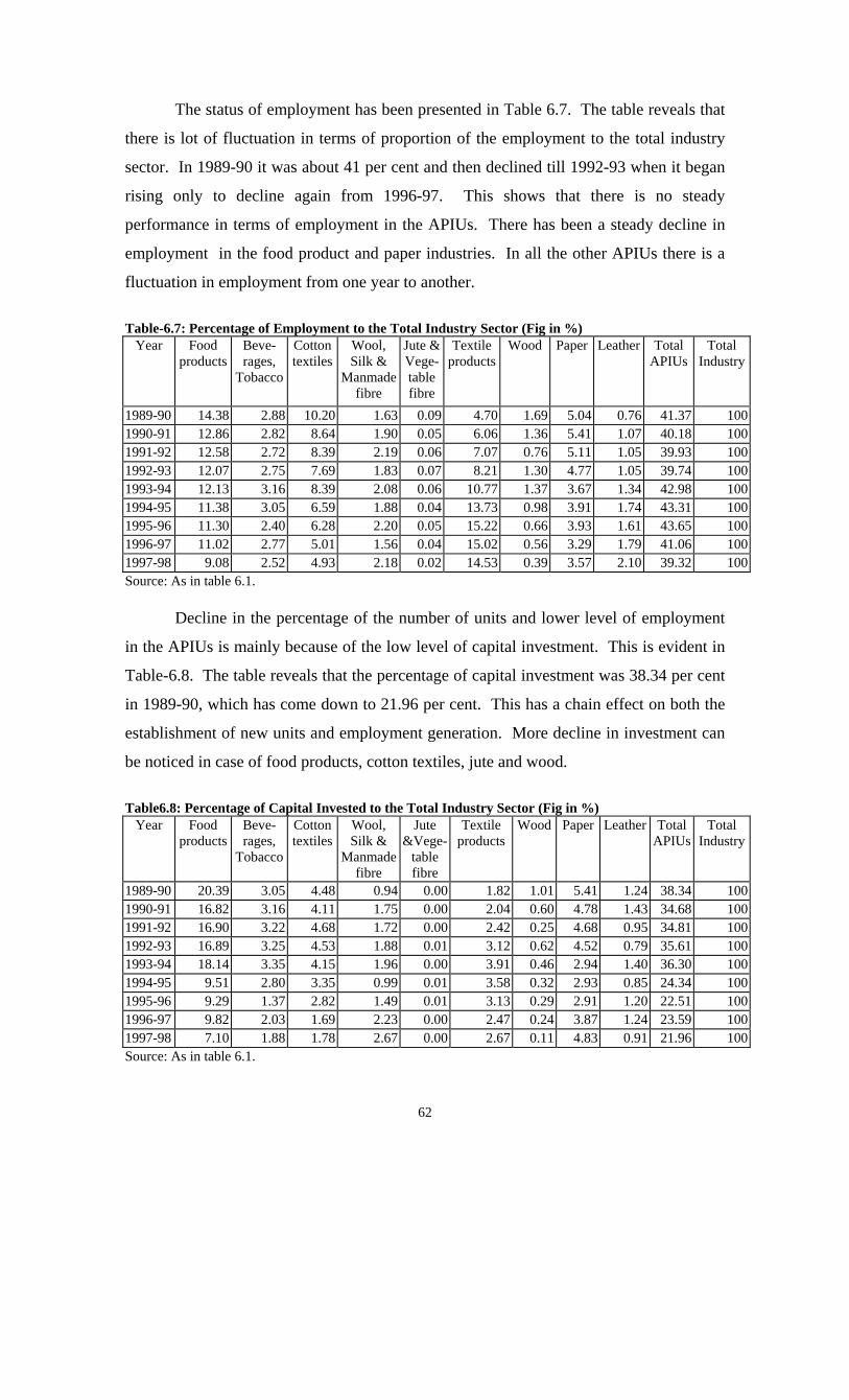
62

The status of employment has been presented in Table 6.7. The table reveals that

there is lot of fluctuation in terms of proportion of the employment to the total industry

sector. In 1989-90 it was about 41 per cent and then declined till 1992-93 when it began

rising only to decline again from 1996-97. This shows that there is no steady

performance in terms of employment in the APIUs. There has been a steady decline in

employment in the food product and paper industries. In all the other APIUs there is a

fluctuation in employment from one year to another.

Table-6.7: Percentage of Employment to the Total Industry Sector (Fig in %)

Year Food products

Beve-rages,

Tobacco

Cotton textiles

Wool, Silk &

Manmade fibre

Jute & Vege-table fibre

Textile products

Wood Paper Leather Total APIUs

Total Industry

1989-90 14.38 2.88 10.20 1.63 0.09 4.70 1.69 5.04 0.76 41.37 1001990-91 12.86 2.82 8.64 1.90 0.05 6.06 1.36 5.41 1.07 40.18 1001991-92 12.58 2.72 8.39 2.19 0.06 7.07 0.76 5.11 1.05 39.93 1001992-93 12.07 2.75 7.69 1.83 0.07 8.21 1.30 4.77 1.05 39.74 1001993-94 12.13 3.16 8.39 2.08 0.06 10.77 1.37 3.67 1.34 42.98 1001994-95 11.38 3.05 6.59 1.88 0.04 13.73 0.98 3.91 1.74 43.31 1001995-96 11.30 2.40 6.28 2.20 0.05 15.22 0.66 3.93 1.61 43.65 1001996-97 11.02 2.77 5.01 1.56 0.04 15.02 0.56 3.29 1.79 41.06 1001997-98 9.08 2.52 4.93 2.18 0.02 14.53 0.39 3.57 2.10 39.32 100Source: As in table 6.1. Decline in the percentage of the number of units and lower level of employment

in the APIUs is mainly because of the low level of capital investment. This is evident in

Table-6.8. The table reveals that the percentage of capital investment was 38.34 per cent

in 1989-90, which has come down to 21.96 per cent. This has a chain effect on both the

establishment of new units and employment generation. More decline in investment can

be noticed in case of food products, cotton textiles, jute and wood.

Table6.8: Percentage of Capital Invested to the Total Industry Sector (Fig in %)

Year Food products

Beve-rages,

Tobacco

Cotton textiles

Wool, Silk &

Manmade fibre

Jute &Vege-

table fibre

Textile products

Wood Paper Leather Total APIUs

Total Industry

1989-90 20.39 3.05 4.48 0.94 0.00 1.82 1.01 5.41 1.24 38.34 1001990-91 16.82 3.16 4.11 1.75 0.00 2.04 0.60 4.78 1.43 34.68 1001991-92 16.90 3.22 4.68 1.72 0.00 2.42 0.25 4.68 0.95 34.81 1001992-93 16.89 3.25 4.53 1.88 0.01 3.12 0.62 4.52 0.79 35.61 1001993-94 18.14 3.35 4.15 1.96 0.00 3.91 0.46 2.94 1.40 36.30 1001994-95 9.51 2.80 3.35 0.99 0.01 3.58 0.32 2.93 0.85 24.34 1001995-96 9.29 1.37 2.82 1.49 0.01 3.13 0.29 2.91 1.20 22.51 1001996-97 9.82 2.03 1.69 2.23 0.00 2.47 0.24 3.87 1.24 23.59 1001997-98 7.10 1.88 1.78 2.67 0.00 2.67 0.11 4.83 0.91 21.96 100Source: As in table 6.1.

63

The output value seems to be showing mixed response. There is a decline in the

percentage of APIUs to the total industry sector. The decline rate is more pronounced in

the case of food products, cotton textiles, jute, wood and paper. However there is a

mixed response in case of all the APIUs (Table 6.9).

Table-6.9: Output Value of the APIUs to the Total Industry Sector (Fig in %)

Year Food products

Beve-rages,

Tobacco

Cotton textiles

Wool, Silk &

Manmade fibre

Jute &Vege-

table fibre

Textile products

Wood Paper Leather Total APIUs

Total Industry

1989-90 17.66 3.68 4.42 0.99 0.00 1.75 0.86 5.60 1.08 36.05 1001990-91 14.21 3.28 4.10 1.68 0.00 1.98 0.56 4.99 1.30 32.11 1001991-92 14.27 3.55 4.38 1.62 0.00 2.45 0.22 4.73 0.89 32.12 1001992-93 13.70 3.50 3.91 1.86 0.01 2.90 0.50 4.67 0.76 31.81 1001993-94 15.39 3.85 3.97 2.15 0.01 5.22 0.42 3.15 1.29 35.44 1001994-95 14.17 2.73 0.68 1.50 0.00 3.63 0.41 0.44 1.14 24.71 1001995-96 13.77 1.49 3.94 1.57 0.00 4.17 0.27 4.48 0.99 30.67 1001996-97 13.08 3.45 2.22 1.72 0.00 3.75 0.27 3.54 1.48 29.52 1001997-98 11.36 3.07 3.02 2.78 0.00 4.76 0.18 3.40 1.42 30.00 100Source: As in table 6.1.

Table 6.10 presents the value addition of the APIUs to the total industry sector in

the state. The value addition has shown the mixed response and there is no consistency

either in terms of increase or decrease. The year 1994-95 seems to be the best year in

terms of value addition in the APIUs. Otherwise for all the other years from 1989-90 to

1990-91 the performance is not steady.

Table-6.10: Percentage of Value Added in the APIUs to the Total Industry Sector (Fig in %)

Year Food products

Beve-rages,

Tobacco

Cotton textiles

Wool, Silk &

Manmade fibre

Jute & Vege-table fibre

Textile products

Wood Paper Leather Total of

APIUs

Total Industry

1989-90 10.06 5.85 4.02 1.04 0.01 1.67 0.37 4.62 0.69 28.34 1001990-91 6.70 3.81 4.06 1.57 0.01 1.93 0.46 0.41 1.00 19.93 1001991-92 6.67 4.85 3.48 1.35 0.01 2.73 0.13 3.91 0.75 23.87 1001992-93 4.67 4.44 2.04 1.92 0.01 2.38 0.18 4.77 0.70 21.11 1001993-94 7.53 5.93 3.32 3.01 0.01 10.02 0.30 4.02 1.00 35.13 1001994-95 18.00 3.05 12.08 3.61 0.01 8.09 0.57 12.78 1.76 59.93 1001995-96 7.34 1.48 3.00 2.16 0.00 4.78 0.17 5.42 0.70 25.05 1001996-97 5.89 6.23 1.61 2.45 0.00 4.38 0.17 3.82 0.90 25.45 1001997-98 9.40 5.15 2.91 6.73 0.00 5.37 0.12 3.01 0.88 33.57 100Source: As in table 6.1.

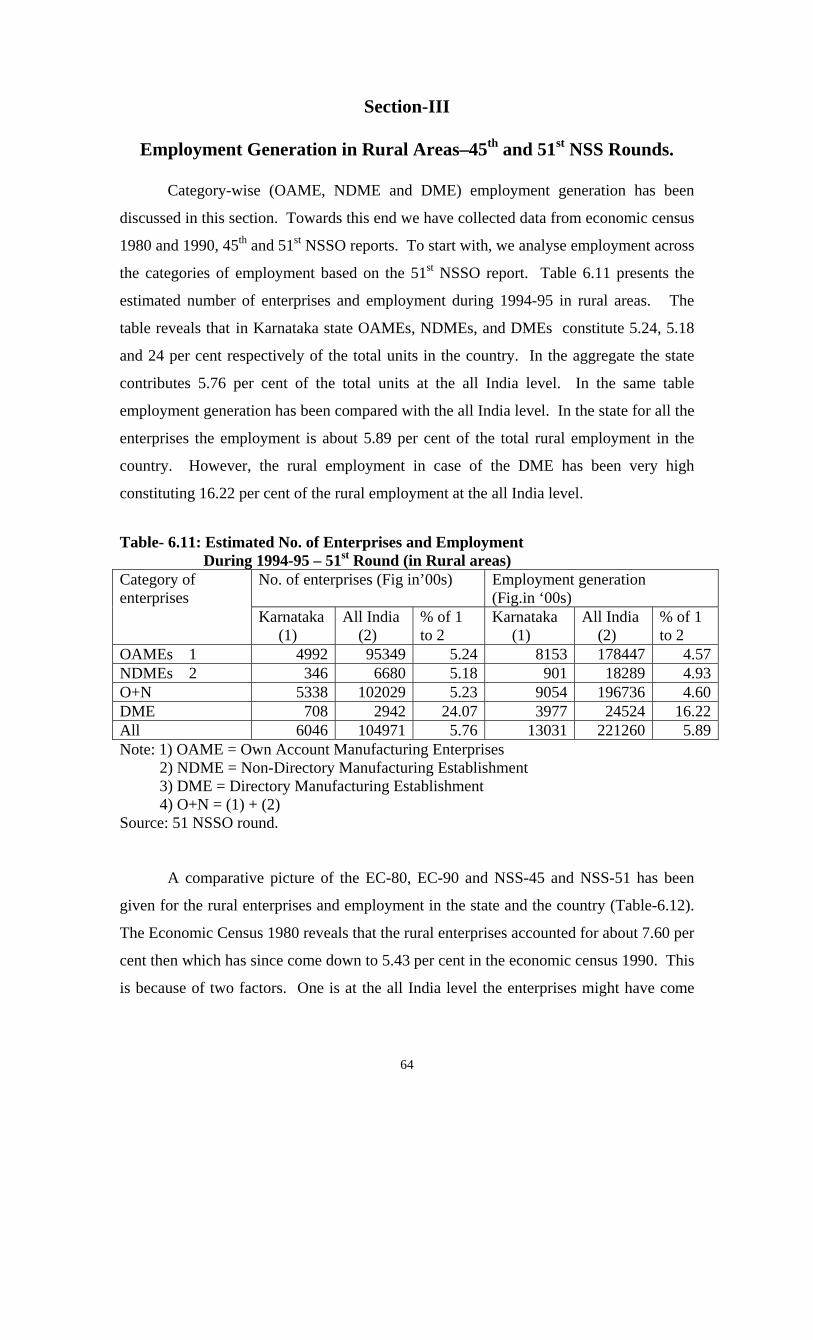
64

Section-III

Employment Generation in Rural Areas–45th and 51st NSS Rounds. Category-wise (OAME, NDME and DME) employment generation has been

discussed in this section. Towards this end we have collected data from economic census

1980 and 1990, 45th and 51st NSSO reports. To start with, we analyse employment across

the categories of employment based on the 51st NSSO report. Table 6.11 presents the

estimated number of enterprises and employment during 1994-95 in rural areas. The

table reveals that in Karnataka state OAMEs, NDMEs, and DMEs constitute 5.24, 5.18

and 24 per cent respectively of the total units in the country. In the aggregate the state

contributes 5.76 per cent of the total units at the all India level. In the same table

employment generation has been compared with the all India level. In the state for all the

enterprises the employment is about 5.89 per cent of the total rural employment in the

country. However, the rural employment in case of the DME has been very high

constituting 16.22 per cent of the rural employment at the all India level.

Table- 6.11: Estimated No. of Enterprises and Employment During 1994-95 – 51st Round (in Rural areas)

No. of enterprises (Fig in’00s) Employment generation (Fig.in ‘00s)

Category of enterprises

Karnataka (1)

All India (2)

% of 1 to 2

Karnataka (1)

All India (2)

% of 1 to 2

OAMEs 1 4992 95349 5.24 8153 178447 4.57NDMEs 2 346 6680 5.18 901 18289 4.93O+N 5338 102029 5.23 9054 196736 4.60DME 708 2942 24.07 3977 24524 16.22All 6046 104971 5.76 13031 221260 5.89Note: 1) OAME = Own Account Manufacturing Enterprises 2) NDME = Non-Directory Manufacturing Establishment 3) DME = Directory Manufacturing Establishment 4) O+N = (1) + (2) Source: 51 NSSO round. A comparative picture of the EC-80, EC-90 and NSS-45 and NSS-51 has been

given for the rural enterprises and employment in the state and the country (Table-6.12).

The Economic Census 1980 reveals that the rural enterprises accounted for about 7.60 per

cent then which has since come down to 5.43 per cent in the economic census 1990. This

is because of two factors. One is at the all India level the enterprises might have come

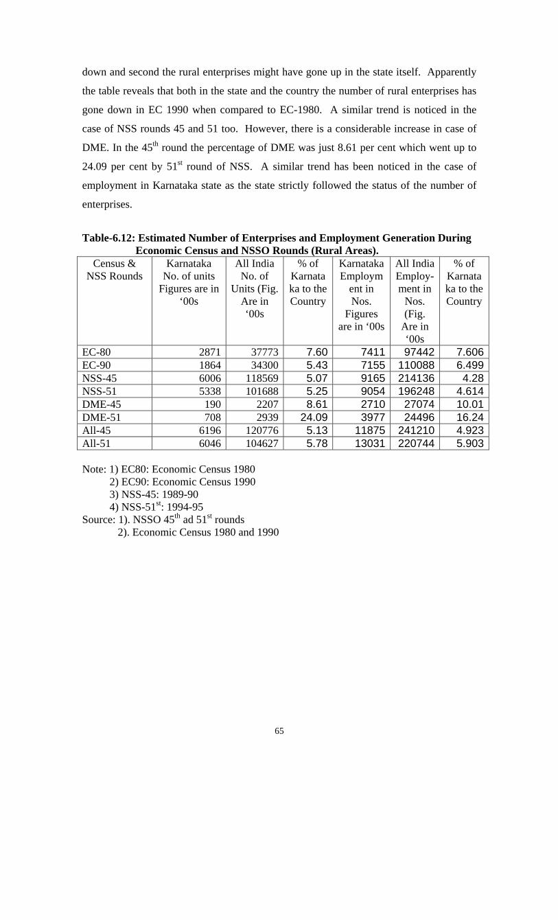
65

down and second the rural enterprises might have gone up in the state itself. Apparently

the table reveals that both in the state and the country the number of rural enterprises has

gone down in EC 1990 when compared to EC-1980. A similar trend is noticed in the

case of NSS rounds 45 and 51 too. However, there is a considerable increase in case of

DME. In the 45th round the percentage of DME was just 8.61 per cent which went up to

24.09 per cent by 51st round of NSS. A similar trend has been noticed in the case of

employment in Karnataka state as the state strictly followed the status of the number of

enterprises. Table-6.12: Estimated Number of Enterprises and Employment Generation During

Economic Census and NSSO Rounds (Rural Areas). Census &

NSS Rounds Karnataka

No. of units Figures are in

‘00s

All India No. of

Units (Fig. Are in ‘00s

% of Karnataka to the Country

Karnataka Employm

ent in Nos.

Figures are in ‘00s

All India Employ-ment in

Nos. (Fig.

Are in ‘00s

% of Karnataka to the Country

EC-80 2871 37773 7.60 7411 97442 7.606EC-90 1864 34300 5.43 7155 110088 6.499NSS-45 6006 118569 5.07 9165 214136 4.28NSS-51 5338 101688 5.25 9054 196248 4.614DME-45 190 2207 8.61 2710 27074 10.01DME-51 708 2939 24.09 3977 24496 16.24All-45 6196 120776 5.13 11875 241210 4.923All-51 6046 104627 5.78 13031 220744 5.903 Note: 1) EC80: Economic Census 1980 2) EC90: Economic Census 1990 3) NSS-45: 1989-90 4) NSS-51st: 1994-95 Source: 1). NSSO 45th ad 51st rounds 2). Economic Census 1980 and 1990

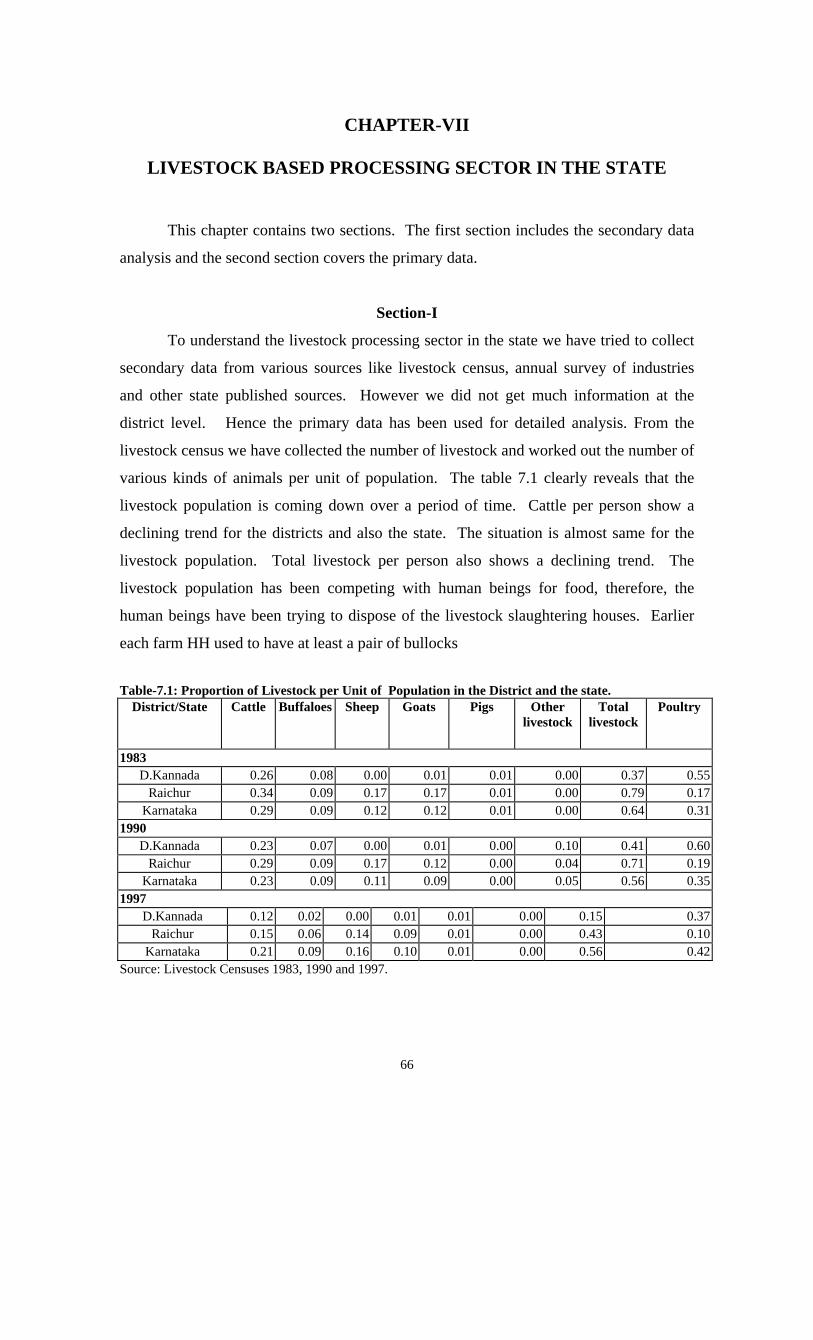
66

CHAPTER-VII

LIVESTOCK BASED PROCESSING SECTOR IN THE STATE

This chapter contains two sections. The first section includes the secondary data

analysis and the second section covers the primary data.

Section-I

To understand the livestock processing sector in the state we have tried to collect

secondary data from various sources like livestock census, annual survey of industries

and other state published sources. However we did not get much information at the

district level. Hence the primary data has been used for detailed analysis. From the

livestock census we have collected the number of livestock and worked out the number of

various kinds of animals per unit of population. The table 7.1 clearly reveals that the

livestock population is coming down over a period of time. Cattle per person show a

declining trend for the districts and also the state. The situation is almost same for the

livestock population. Total livestock per person also shows a declining trend. The

livestock population has been competing with human beings for food, therefore, the

human beings have been trying to dispose of the livestock slaughtering houses. Earlier

each farm HH used to have at least a pair of bullocks

Table-7.1: Proportion of Livestock per Unit of Population in the District and the state.

District/State Cattle Buffaloes Sheep Goats Pigs Other livestock

Total livestock

Poultry

1983 D.Kannada 0.26 0.08 0.00 0.01 0.01 0.00 0.37 0.55

Raichur 0.34 0.09 0.17 0.17 0.01 0.00 0.79 0.17Karnataka 0.29 0.09 0.12 0.12 0.01 0.00 0.64 0.31

1990 D.Kannada 0.23 0.07 0.00 0.01 0.00 0.10 0.41 0.60

Raichur 0.29 0.09 0.17 0.12 0.00 0.04 0.71 0.19Karnataka 0.23 0.09 0.11 0.09 0.00 0.05 0.56 0.35

1997 D.Kannada 0.12 0.02 0.00 0.01 0.01 0.00 0.15 0.37

Raichur 0.15 0.06 0.14 0.09 0.01 0.00 0.43 0.10Karnataka 0.21 0.09 0.16 0.10 0.01 0.00 0.56 0.42

Source: Livestock Censuses 1983, 1990 and 1997.

67

but now the bullocks are hardly seen in the villages (Rajendran 1994). The table 7.2

presents the production of animal products like milk, meat, pork, etc. As the number of

livestock is coming down the production of meat is growing positively. Production of

cattle and buffalo has grown at the rate of about 10 and 12 per cent respectively. Though

the pig population is less per unit of human population, the pork production is growing at

the rate of 18 per cent.

Table-7.2: Production and its GR of the Livestock in Karnataka

Year Milk Production '000 tonnrs

Production of Mutton

'00 tonnes

Production of Beef '00 tonnes

Chicken meat

'00 tonnes Cow Buffa-

loes

Wool in tonnes

Sheep Goat Cattle Buffaloes

Pork '00 tonnrs

Egg in lakhs

989-90 1240 1040 3736 225 175 6949 4397 2154 12780 NA 990-91 1284 1094 3806 233 2040 2337 1242 505 7320 NA 991-92 1322 1142 3892 236 185 7297 4717 2476 13362 NA 992-93 1390 1188 3926 242 189 7679 4828 2536 13490 NA 993-94 1461 1262 3978 249 192 7995 6247 2598 14169 NA 1994-95 1631 1358 4046 253 198 8206 7512 3341 14699 NA 1995-96 1747 1427 4098 267 206 8966 8176 3586 15579 NA 1996-97 1916 1526 4229 272 212 9996 6654 5554 16303 NA 1997-98 2347 1601 4691 285 218 10821 6657 4604 18124 NA 1998-99 2539 1661 5205 306 232 11291 7231 4933 19380 NA 2001-02 2744 1990 5757 331 224 12614 8919 6403 20273 13956GR in % 8.76 6.14 3.85 3.60 -5.88 10.62 12.06 18.12 7.14 --- Source: Various Issues of Annual Survey of Industries. The percentage of livestock processing enterprises in the state to the country has

been presented in table 7.3. The table reveals that the percentage of slaughtering and the

preservation of meat factories was just 0.09 per cent in the state. The net income from

this and animal oils and fats is negative. However, the manufacture of dairy products

and processing, canning and preservation of fish the net income is positive. This shows

that Karnataka state’s performance in terms of livestock processing activity is not

significant. Table-7.3: Percentage of Livestock Processing Enterprises in the State to the Country (1991-92)

Characteristics Slaughtering, Preparation, and

Preservation of meat

Manufacture of Dairy products

Processing, Canning &

preservation of Fish

Manufacture of animal oils & fats, fish oil & food products

Total All India

Number of Factories 0.09 0.63 0.36 1.50 5850Fixed capital 0.13 0.75 0.08 0.64 47915601Total persons engaged 0.03 0.70 0.40 0.43 433848Total inputs 0.09 1.73 0.51 0.61 111961017Value of output 0.06 1.45 0.43 0.46 151736369Net income -0.09 0.75 0.10 -0.13 24930865Source: As in table 7.2.

68

Aquaculture in the State: Fishing is one of the most important occupations in coastal Karnataka. The major

fish producing districts are Udupi, DK and UK. Of these most of the fish is accounted

for by DK district. However, the district-wise details are not available and therefore, we

have tried to give the aggregate picture of the aquaculture in the state. Fish production is

growing at the rate of 0.23 per cent whereas the fish value is growing at the rate of 8.79

per cent (Table 7.4). However the absolute figures reveal that the value of fish has been

coming down in the last two years, i.e., from 2001-02 to 2002-03. The proportion of

marine fish varied between 41.01 per cent in 2001-02 to 77.44 per cent in the succeeding

year. Approximately around 4 per cent of the total fish is being exported to many

countries of the world. Growth rate of total fish production and fish value has been

presented in table 7.5. It is clear from the table that marine fish production is declining at

the rate of 2.3 per cent, whereas inland fish production is growing at the rate of 4.74 per

cent. Overall production has stagnated but the value is growing; this may be due to

increase in the price of fish products. The export quantity showed increasing trend but

not the value earned from the fish exports. Table-7.4: Fish Production and its Value in the State

Year Quantity in Metric Tonnes

Value Rs. in Lakhs

% of Marine fish

% of Marine fish value

% of Export quantity

% of export quantity value

1993-94 249154 21906 70.046 65.932 3.262 34.6981994-95 242787 25659 71.050 72.606 3.748 44.0891995-96 304865 36554 71.347 76.104 2.348 27.0131996-97 324423 33990 68.669 70.090 3.056 29.2041997-98 310401 52037 61.166 45.435 3.399 22.5451998-99 279046 49004 57.563 42.872 4.210 23.2541999-00 292299 53390 56.672 44.360 4.412 22.9222000-01 305375 54740 58.259 45.358 3.872 17.2562001-02 249612 48285 51.446 41.301 3.778 13.1262002-03 266423 43458 67.622 77.438 3.674 14.428GR in % 0.234 8.792 -- -- -- -- Source: Statistical Bulletin of Fisheries, DES, Government of Karnataka, Bangalore (2002-03). Table-7.5: GR of Fish Production and the Value

Source of fish GR in % 1993-94 to 2002-03 Marine Fish -2.3008Value 9.0464Inland Fish 4.7445Value 13.9686Total 0.2344Value 8.7922Export Qty. 3.2827Value -3.2261Source: As in table 7.4.

69

Only fish production at the district level is available but not any other details.

Table 7.6, presents the fish production across the districts and the state. In Raichur we do

not have any marine fish. Even the percentage share of inland fish is not that high.

However, the percentage share is increasing every year. In DK district the percentage

share of marine fish is very high. It is almost 40 per cent of the state’s total production.

However, the percentage share of inland fish is very low, around just 1 per cent.

Table-7.6: Proportion of fish production in the sample districts

District/State 1999-00 2000-01 2001-02 2002-03

Raichur Marine 0 0 0 0Inland 2.74 2.68 2.83 3.01Total 1.19 1.12 1.38 0.98D.Kannada Marine 40.53 45.13 37.32 45.56Inland 0.91 0.87 0.94 1.26Total 23.36 26.66 19.66 31.21Karnataka Marine* 165653 177907 128416 180161Inland* 126646 127468 121196 86262Total* 292299 305375 249612 266423Note: * Metric tones Source: As in table 7.4.

Section-II

In this section we have given the primary data analysis and the field observations

relating to livestock activities like leather products and fishing activities in both the

districts being studied.

Production and Employment Situation of Livestock Enterprises:

In Raichur district we have three categories of enterprises: Own Account

Manufacturing Enterprises (OAME), Non-Directory Manufacturing Enterprises (NDME)

and Directory Manufacturing Enterprises (DME). In DK district the factory sector is also

included in addition to these three categories of enterprises. This categorisation has been

made based on the size of enterprise in terms of employment. In total we have collected

data from 12 and 15 enterprises in both Raichur and DK districts respectively. In

Raichur, cow, bullock, buffalo, and other animals’ leather-related works are done. In DK

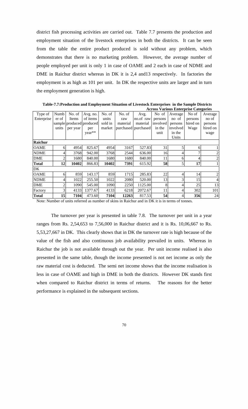
70

district fish processing activities are carried out. Table 7.7 presents the production and

employment situation of the livestock enterprises in both the districts. It can be seen

from the table the entire product produced is sold without any problem, which

demonstrates that there is no marketing problem. However, the average number of

people employed per unit is only 1 in case of OAME and 2 each in case of NDME and

DME in Raichur district whereas in DK it is 2,4 and13 respectively. In factories the

employment is as high as 101 per unit. In DK the respective units are larger and in turn

the employment generation is high.

Table-7.7:Production and Employment Situation of Livestock Enterprises in the Sample Districts

Across Various Enterprise Categories Type of

Enterprise Number of

sample units

No. of Items

produced per year

Avg. no. of items produced

per year**

No. of units

sold in market

No. of raw

material purchased

Avg. no.of raw material

purchased

No of persons involved

in the unit

Average no of

persons involved

in the Units

No of persons hired on Wage

Average no of

persons hired on

wage

Raichur OAME 6 4954 825.67 4954 3167 527.83 31 5 6 1NDME 4 3768 942.00 3768 2544 636.00 16 4 7 2DME 2 1680 840.00 1680 1680 840.00 11 6 4 2Total 12 10402 866.83 10402 7391 615.92 58 5 17 1DK OAME 6 859 143.17 859 1715 285.83 22 4 14 2NDME 4 1022 255.50 1022 2080 520.00 13 3 15 4DME 2 1090 545.00 1090 2250 1125.00 8 4 25 13Factory 3 4133 1377.67 4133 6218 2072.67 11 4 302 101Total 15 7104 473.60 7104 12263 817.53 54 4 356 24

Note: Number of units referred as number of skins in Raichur and in DK it is in terms of tonnes. The turnover per year is presented in table 7.8. The turnover per unit in a year

ranges from Rs. 2,54,653 to 7,56,000 in Raichur district and it is Rs. 10,06,667 to Rs.

5,53,27,667 in DK. This clearly shows that in DK the turnover rate is high because of the

value of the fish and also continuous job availability prevailed in units. Whereas in

Raichur the job is not available through out the year. Per unit income realised is also

presented in the same table, though the income presented is not net income as only the

raw material cost is deducted. The semi net income shows that the income realisation is

less in case of OAME and high in DME in both the districts. However DK stands first

when compared to Raichur district in terms of returns. The reasons for the better

performance is explained in the subsequent sections.

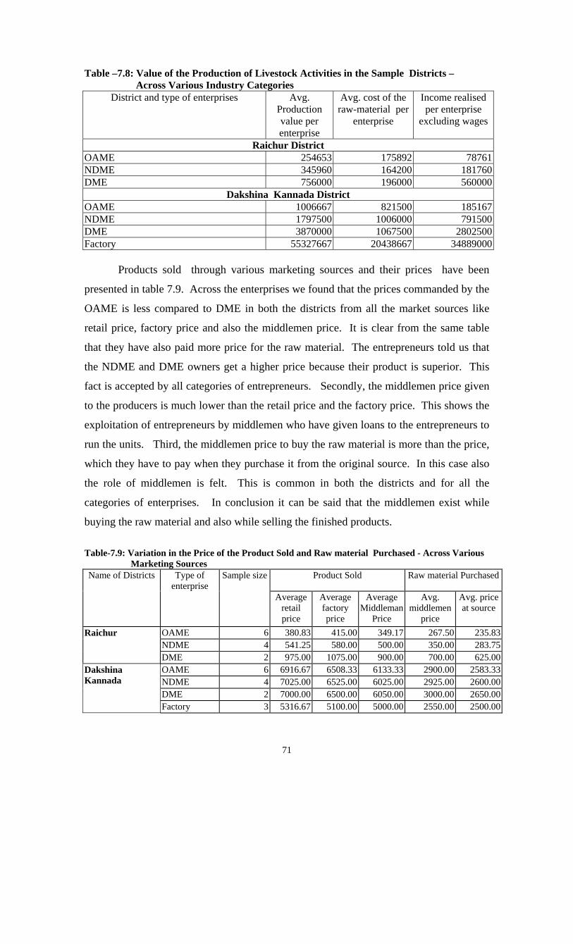
71

Table –7.8: Value of the Production of Livestock Activities in the Sample Districts – Across Various Industry Categories

District and type of enterprises Avg. Production value per enterprise

Avg. cost of the raw-material per

enterprise

Income realised per enterprise

excluding wages

Raichur District OAME 254653 175892 78761NDME 345960 164200 181760DME 756000 196000 560000

Dakshina Kannada District OAME 1006667 821500 185167NDME 1797500 1006000 791500DME 3870000 1067500 2802500Factory 55327667 20438667 34889000 Products sold through various marketing sources and their prices have been

presented in table 7.9. Across the enterprises we found that the prices commanded by the

OAME is less compared to DME in both the districts from all the market sources like

retail price, factory price and also the middlemen price. It is clear from the same table

that they have also paid more price for the raw material. The entrepreneurs told us that

the NDME and DME owners get a higher price because their product is superior. This

fact is accepted by all categories of entrepreneurs. Secondly, the middlemen price given

to the producers is much lower than the retail price and the factory price. This shows the

exploitation of entrepreneurs by middlemen who have given loans to the entrepreneurs to

run the units. Third, the middlemen price to buy the raw material is more than the price,

which they have to pay when they purchase it from the original source. In this case also

the role of middlemen is felt. This is common in both the districts and for all the

categories of enterprises. In conclusion it can be said that the middlemen exist while

buying the raw material and also while selling the finished products.

Table-7.9: Variation in the Price of the Product Sold and Raw material Purchased - Across Various

Marketing Sources Product Sold Raw material PurchasedName of Districts Type of

enterprise Sample size

Average retail price

Average factory price

Average Middleman

Price

Avg. middlemen

price

Avg. price at source

OAME 6 380.83 415.00 349.17 267.50 235.83NDME 4 541.25 580.00 500.00 350.00 283.75

Raichur

DME 2 975.00 1075.00 900.00 700.00 625.00OAME 6 6916.67 6508.33 6133.33 2900.00 2583.33NDME 4 7025.00 6525.00 6025.00 2925.00 2600.00DME 2 7000.00 6500.00 6050.00 3000.00 2650.00

Dakshina Kannada

Factory 3 5316.67 5100.00 5000.00 2550.00 2500.00

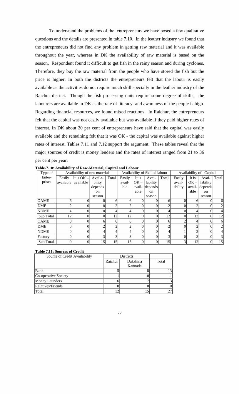
72

To understand the problems of the entrepreneurs we have posed a few qualitative

questions and the details are presented in table 7.10. In the leather industry we found that

the entrepreneurs did not find any problem in getting raw material and it was available

throughout the year, whereas in DK the availability of raw material is based on the

season. Respondent found it difficult to get fish in the rainy season and during cyclones.

Therefore, they buy the raw material from the people who have stored the fish but the

price is higher. In both the districts the entrepreneurs felt that the labour is easily

available as the activities do not require much skill specially in the leather industry of the

Raichur district. Though the fish processing units require some degree of skills, the

labourers are available in DK as the rate of literacy and awareness of the people is high.

Regarding financial resources, we found mixed reactions. In Raichur, the entrepreneurs

felt that the capital was not easily available but was available if they paid higher rates of

interest. In DK about 20 per cent of entrepreneurs have said that the capital was easily

available and the remaining felt that it was OK - the capital was available against higher

rates of interest. Tables 7.11 and 7.12 support the argument. These tables reveal that the

major sources of credit is money lenders and the rates of interest ranged from 21 to 36

per cent per year. Table-7.10: Availability of Raw-Material, Capital and Labour

Availability of raw material Availability of Skilled labour Availability of Capital Type of Enter- prises

Easily available

It is OK –available

Availa-bility

depends on

season

Total Easily avail-

ble

It is OK –avail-able

Avai-lability depends

on season

Total Easily avail-ability

It is OK –avail-able

Avai-lability depends

on season

Total

OAME 6 0 0 6 6 0 0 6 0 6 0 6DME 2 0 0 2 2 0 0 2 0 2 0 2NDME 4 0 0 4 4 0 0 4 0 4 0 4 Sub Total 12 0 0 12 12 0 0 12 0 12 0 12OAME 0 0 6 6 6 0 0 6 2 4 0 6DME 0 0 2 2 2 0 0 2 0 2 0 2NDME 0 0 4 4 4 0 0 4 1 3 0 4Factory 0 0 3 3 3 0 0 3 0 3 0 3 Sub Total 0 0 15 15 15 0 0 15 3 12 0 15

Table 7.11: Sources of Credit

Source of Credit Availability Districts Raichur Dakshina

Kannada Total

Bank 5 8 13 Co-operative Society 1 0 1 Money Launders 6 7 13 Relatives/Friends 0 0 0 Total 12 15 27

73

Table-7.12: Rate of Interest Charged on Loans. Districts Rate of Interest on Loan

Raichur Dakshina Kannada

Total

11-15% 6 8 14 16-20% 0 0 0 21-36% 6 7 13 Above 36% 0 0 0 Total

12 15 27

In the case of availability of infrastructure 50 per cent of the entrepreneurs felt

that it was moderate and 25 per cent each said that it was poor and better in Raichur

district (Table 7.13). In DK 60 per cent of the entrepreneurs felt that the infrastructure has

better and 20 per cent each have felt that it was moderate or best. This clearly shows that

the infrastructure availability in Raichur is poor and DK it is better. The same trend is

applicable to the availability of supporting equipment. Tables 7.14 and 7.15 present the

pattern of demand for the products which they produce and also the quality consciousness

of the buyers. Here also we found that the DK’s performance is better compared to

Raichur district. It is no wonder that Raichur’s performance is poor and DK’s

performance best in terms of turnover, output and the price for the goods which they

produce.

Table – 7.13:Availability of Supporting Infrastructure and Equipment

Availability of Supporting Infrastructure Availability of supporting equipment

Opinion of the respondents

Raichur Dakshina Kannada

Total Raichur Dakshina Kannada

Total

Poor 3 0 3 0 0 0OK/ Moderate 6 3 9 12 4 16Better 3 9 12 0 11 11Best 0 3 3 0 0 0Total 12 15 27 12 15 27 Table-7.14: Size and Pattern of Demand

Size and Pattern of Demand Raichur Dakshina Kannada

Total

Poor 0 0 0Normal 12 9 21Better 0 6 6Best 0 0 0Total 12 15 27

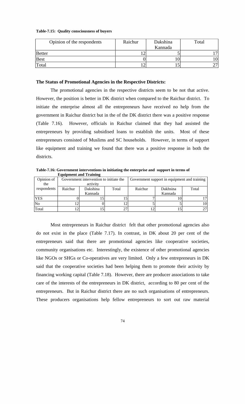
74

Table-7.15: Quality consciousness of buyers

Opinion of the respondents Raichur Dakshina Kannada

Total

Better 12 5 17Best 0 10 10Total 12 15 27 The Status of Promotional Agencies in the Respective Districts:

The promotional agencies in the respective districts seem to be not that active.

However, the position is better in DK district when compared to the Raichur district. To

initiate the enterprise almost all the entrepreneurs have received no help from the

government in Raichur district but in the of the DK district there was a positive response

(Table 7.16). However, officials in Raichur claimed that they had assisted the

entrepreneurs by providing subsidised loans to establish the units. Most of these

entrepreneurs consisted of Muslims and SC households. However, in terms of support

like equipment and training we found that there was a positive response in both the

districts.

Table-7.16: Government interventions in initiating the enterprise and support in terms of

Equipment and Training Government intervention to initiate the

activity Government support in equipment and trainingOpinion of

the respondents Raichur Dakshina

Kannada Total Raichur Dakhsina

Kannada Total

YES 0 15 15 7 10 17No 12 0 12 5 5 10Total 12 15 27 12 15 27 Most entrepreneurs in Raichur district felt that other promotional agencies also

do not exist in the place (Table 7.17). In contrast, in DK about 20 per cent of the

entrepreneurs said that there are promotional agencies like cooperative societies,

community organisations etc. Interestingly, the existence of other promotional agencies

like NGOs or SHGs or Co-operatives are very limited. Only a few entrepreneurs in DK

said that the cooperative societies had been helping them to promote their activity by

financing working capital (Table 7.18). However, there are producer associations to take

care of the interests of the entrepreneurs in DK district, according to 80 per cent of the

entrepreneurs. But in Raichur district there are no such organisations of entrepreneurs.

These producers organisations help fellow entrepreneurs to sort out raw material

75

problems, fixation of price for their products, protect entrepreneurs from middlemen by

giving raw material and also credit and fixing wages for the labourers (Table 7.19). Table-7.17:Existence of Promotional Agencies

Opinion of the respondents Raichur Dakshina Kannada

Total

Yes 0 3 3No 12 12 24Total 12 15 27 Table-7.18: Existence of NGOs or SHGs or Co-operative Societies

Opinion of the respondents Raichur Dakhsina Kannada

Total

Yes 0 4 4No 12 11 23Total 12 15 27 Table-7.19: Existence of Producer Associations

Opinion of the respondents Raichur Dakshina Kannada

Total

Yes 0 12 12No 12 3 15Total 12 15 27 Conclusions: The secondary data analysis reveals that the agricultural employment for males

keeps on declining and the NFE goes on increasing. However, in case of the female

labourers the agriculture employment has come down but at a lower rate when compared

to the male. The NFE in general for the females has shown stagnation with symptoms of

declining. Growth rate in the employment of the rural people has come down from 2.12

per cent to 0.17 per cent in Karnataka state and the similar trends are noticed even at the

all India level.

The district and the village level analysis reveals that the NFE is not based on the

growth related factors like agriculture development. Because though Raichur district has

76

been one of the agriculturally developed district the NFE has been much low when

compared to the other districts. The agriculture development can be explained in terms of

the availability of irrigation facilities, land-man ratio, cropped area, etc. The distress

diversification hypothesis holds good partially in DK district because in DK, the NFE is

very high, this can be explained due to distress factors like land-man ratio and the

cropped area, and the non-availability of irrigation facilities. However, the major factors

to determine the NFE are the literacy rate, people’s awareness, willingness to work and

the availability of infrastructure facilities. In DK the literacy rate is high, infrastructure

availability is more, the people are well aware of the problems and they have willingness

to work and therefore, NFE is high. In addition to these the NFE in DK district is not as a

last resort, which is mentioned in the distress diversification hypothesis, because, people

have been opting for this occupation as it pays more when compared to other occupations

specially agricultural labour in rural areas.

In general, the regular-employment has been more in DK district when compared

to Raichur district. In case of self-employment, our observation revealed that DK district

has an edge over Raichur district but in terms of data both the districts seem to be the

same. The number of casual labourers are more in DK district compared to Raichur

district. In fact the casualisation of labour has been increasing compared to regular and

self-employment in both the districts.

77

REFERENCES

Acharya, S. and A. Mitra (2000). The Potential of Rural Industries and Trade to Provide Decent Work Conditions: A Data Reconnaissance in India. SAAT Working Papers, New Delhi: International Labour Organization. Anderson, Dennis and Leisonson, W. Mark (1980). Rural Non-farm Employment in Developing Countries. Economic and Cultural Change, 28(2). Basant R., B.L. Kumar and R. Parthasarathy (1998). Non-Agricultural Employment in Rural India: The Case of Gujarat (ed.,). Jaipur: Rawat Publications. Basu and Kashyap (1992). Rural Non-Agricultural Employment in India: Role of Development Process and Rural Urban Employment Linkages. Economic and Political Weekly, XXVII(51-52), December 19-26. Bhalla, G. and Peter Hazell (2003). Rural Employment and Poverty Strategies to Eliminate Rural Poverty Within a Generation. Economic and Political Weekly, XXXVIII(33): 3473-84. Chadha, G.K. (1986). Agricultural Growth and Rural Non-Farm Activities: An Analysis of Indian Experience. In Yang-Boo Choe and Fu-chen Lo (Eds.). Rural Industrialisation and Non-Farm Activities of Asian Farmers, Korea Rural Economics Institute, Asian and Pacific Development Centre. Chadha, G.K. (2001). Impact of Economic Reforms on Rural Employment: No Smooth Sailing Anticipated. Indian Journal of Agricultural Economics, 56(3): 491. Chadha, G.K. and P.P. Sahu (2002). Post-Reform Setbacks in Rural Employment – Issues that need Further Scrutiny. Economic and Political Weekly, XXXVI(21): 1998-2026. Dev, Mahendra, S (1990). Non-Agricultural Employment in Rural India: Evidence at a Dis-aggregate Level. Economic and Political Weekly, July 14. Dev, Mahendra, S. (2003). Agriculture, Employment and Social Sector Neglected. Economic and Political Weekly, XXXVIII(14 & 13): 1353-56. Edgreen, G. and M. Muqtada (1989). Strategies for Growth and Employment in Asia: Learning from within, ARTEP Working Papers. Gayathri, K. (2003). Who Benefits from Industrial Incentives – A Study of Capital Investment Subsidy in Karnataka. ISEC Working Paper No. 124, Bangalore. Government of Karnataka GOK (1993). Report of the Expert Committee on Stagnation of Agricultural Productivity in Karnataka During 1980s (Chairman: T.R. Satish Chandran). Government of Karnataka).

78

Liedholm, Carl and Peter Kilby (1989). The Role of Non-Farm Activities in the Rural Economy. In Jafferey G. William and V.R. Panchamukhi (Eds.). The Balance Between the Industry and Agriculture in Economic Development: Sector Proportions, Vol. 2, ILO/Macmilan Press, London. Papola, T.S. (1987). Rural Industrialisation and Agricultural Growth: A Case Study on India. In R.Islam (ed). Rural Industrialisation and Employment in Asia, ILO/ARTEP, New Delhi. Raj, K.N. (1976). Growth and Stagnation in Indian Industrial Development. Economic and Political Weekly, 11(5,6&7). Rajasekhar, D., (1991). Non-Farm Sector in India: Issues and Evidence. Paper Presented in National Consultation on Identification of Research Priorities in Non-far Sector, Institute for Social and Economic Change, Bangalore. Rajasekhar, D. (1995). Pattern and Determinants of Rural Non-Farm Employment in Karnataka: A Disaggregated Analysis at District Level. Agricultural Situation in India, LII: 279-86. Rajasekhar, D. and B.R.Biradar (1998). Rural Non-Farm Activities in Karnataka. Unpublished Report, Agriculture Development and Rural Transformation Unit, Institute for Social and Economic Change. Rajendran, S. (1993). Changing Patterns of Farm Power use in Agriculture – A Study of Tamil Nadu Villages. Ph.D. Thesis, Bangalore: Institute for Social and Economic Change. Samuel P.S. HO (1979). Decentralised Industrialisation and Rural Development: Evidence From Taiwan. Economic Development and Cultural Change, 20(1). Unni, Jeemol, (1991). Regional Variations in Rural Non-Agricultural Employment: An Exploratory Analysis. Economic and Political Weekly, January, 19. Vaidyanathan A. (1986). Labour Use in Rural India: A Study of Spatial and Temporal Variations.” Economic and Political Weekly, XXI(52), December 27. Visaria, P. and R. Basant (1994). Non Agricultural Employment in India: Problems and Perspective. In Visaria, P. and Basant, R. (eds.). Non Agricultural Employment in India, New Delhi: Sage Publications. Vyasulu, Vinod (1990). The Non-Farm Sector in the Indian Economy: A Discussion Note on Research Priorities. Indian Journal of Social Science, July-September.