rwth aachen university master thesis modeling and
TRANSCRIPT

RWTH Aachen University
Simulation Science
Master’s Thesis
Modeling and simulation of
heat source trajectories through
phase-change materials
Alexander Gary Zimmerman
Matriculation-no. 351345
First reviewer: Prof. Marek Behr, Faculty of Mechanical Engi neering
Second reviewer: Dr. Julia Kowalski, Junior Research Group Leader, AICES
Aachen, November 2016

Statutory declaration
I, Alexander Gary Zimmerman, declare that I have independently authored this thesis, that I
have only used the declared sources, and that I have explicitly marked all material which has
been quoted either literally or by content from these sources.
Aachen, November 2016
Alexander Gary Zimmerman

Abstract
The modeling and simulation of heat source trajectories through phase-change materials is a
relevant problem both for space exploration and for terrestrial climate research, among other
fields. In space, the DLR and NASA are both interested in exploring beneath the surfaces of icy
moons, primarily Enceladus and Europa, where conditions may allow for extraterrestrial life. On
Earth, unique subglacial aquatic ecosystems offer potential for geobiological discoveries.
Unfortunately, existing ice-drilling technology is dirty and cumbersome. Most importantly, the
target environments must not be contaminated; but furthermore, such heavy equipment cannot
be reasonably landed for extraterrestrial missions. Melting probes are a clean and compact
alternative technology which use heaters to melt through the ice. In recent years, the IceMole
melting probe has been developed and deployed. Unique to the IceMole, its trajectory is
controlled with differential heating and a small stabilizing drill, allowing the probe to avoid
obstacles and navigate to distant targets.
Successful melting probe trajectory control requires advancements not only in the modeling and
simulation of the ambient dynamics, e.g. the transport of mass, momentum, and energy within a
phase-change material (PCM) domain, but also of the melting probe’s coupled rigid body
dynamics (RBD). Fundamentally the RBD can be modeled by the equations of motion with force
and moment balances; but this approach has already been shown as prohibitively complex for
the efficient computation of the coupled RBD and ambient dynamics. In this work, we propose
a new approach which views the heat source moving through a series of states that are in
equilibrium with the ambient dynamics. Most significantly, the motion of the probe is driven by
contact with the evolving phase-change interface (PCI) as the probe melts through the material.
From this perspective, the RBD are formulated as an energy minimization problem. For the
ambient dynamics, in this work, we do not yet employ a realistic phase-change model, but rather
we use a simplified model which yields a qualitatively interesting PCI. This allows us to test the
coupled problem before investing in the implementation of more advanced phase-change models.
This thesis formulates the general mathematical problem as two split operators, one for the RBD
and one for the ambient dynamics. We couple these operators with feasibility constraints. The
constraints ensure that the probe does not penetrate the evolving solid PCM domain. Then we
provide a concrete example both for the energy minimization problem, which we formulate and
implement as a nonlinear program, and for the unsteady ambient dynamics, which we formulate
as a partial differential equation (PDE) and implement as a discrete linear system. In addition to
verifying the correctness of the PDE implementation, special care is taken to verify its spatial
and temporal orders of accuracy. Finally, we present an algorithm for the temporal coupling of
the split operators, which we implement in Python and C++. We demonstrate example
trajectories, including the dynamic response of the RB velocity to a rapid change in the heat flux.

Contents
List of figures and tables ............................................................................................................... I
Nomenclature ............................................................................................................................... II
1 Background and introduction ................................................................................................1
1.1 Melting probes for subglacial exploration ....................................................................1
1.2 The physical forward problem ......................................................................................2
1.3 Inverse problems ...........................................................................................................3
1.4 Objectives and outline ...................................................................................................4
2 Previous work and existing methods ....................................................................................5
2.1 The melting process ......................................................................................................5
2.1.1 The one-dimensional Stefan problem ...................................................................5
2.1.2 The enthalpy-porosity model ................................................................................6
2.2 Migrating heat sources through phase-change materials ..............................................7
3 General mathematical formulation of the physical problem .................................................9
3.1 ℋ: Rigid-body dynamics ............................................................................................11
3.2 ℒ: Ambient dynamics ..................................................................................................12
4 ℋ: Equilibrium motion modeled as energy minimization ..................................................14
4.1 The general minimization form ...................................................................................15
4.2 Minimize gravitational potential subject to feasibility constraints .............................15
4.2.1 Feasibility constraints 𝒈: No solid penetration ...................................................15
4.2.2 Energy function 𝒇: gravitational potential ..........................................................16
4.3 ℋ as a constrained nonlinear program ........................................................................18
4.3.1 Local vs. global optimization, and gradient-based vs. gradient-free ..................19
4.3.2 Python implementation .......................................................................................20
4.3.3 Tracking a moving phase-change interface .........................................................23
5 ℒ: Unsteady convection-diffusion of a temperature field ...................................................25
5.1 The strong form ...........................................................................................................25
5.2 Discretization via the finite element method (FEM) ...................................................26
5.2.1 The weak form and spatial discretization ............................................................26
5.2.2 Time discretization ..............................................................................................27
5.2.3 The issue of discretizing asymmetric operators with FEM .................................29

6 Peclet: An implementation of ℒ in C++ with deal.II .......................................................... 30
6.1 deal.II basics ............................................................................................................... 30
6.1.1 Matrix assembly and linear solvers .................................................................... 31
6.1.2 Mesh refinement, input/output, parallel computing, and compiler support ........ 32
6.2 Developments in the Peclet code ................................................................................ 33
6.2.1 Assembling the convection-diffusion matrix ...................................................... 34
6.2.2 Grid generation and refinement .......................................................................... 34
6.2.3 Generalizing the handling of functions............................................................... 36
6.3 Verification ................................................................................................................. 37
6.3.1 Comparison to unsteady 1D model problem from Donea & Huerta .................. 37
6.3.2 1D exact steady solution ..................................................................................... 38
6.3.3 1D unsteady manufactured solution ................................................................... 40
6.3.4 2D unsteady manufactured solution ................................................................... 42
7 A realistic phase-change model: Moving melt film ........................................................... 44
7.1.1 Modeling the domain near a melt film boundary ............................................... 44
7.1.2 Sensitivity of the melt film boundary ................................................................. 46
8 Coupling ℋ and ℒ: The complete forward problem .......................................................... 48
8.1 Temporal coupling ...................................................................................................... 48
8.2 The overall trajectory simulator software system ....................................................... 50
8.3 Implementation of the interface to ℒ in deal.II ........................................................... 51
8.3.1 Grid transformation ............................................................................................ 52
8.3.2 Interpolation and extrapolation ........................................................................... 52
8.3.3 Restarting onto a transformed grid with a finite element field function ............. 54
8.3.4 Sampling the finite element solution outside of the solver ................................. 54
8.4 Example results for the coupled trajectory ................................................................. 56
8.4.1 Coupled position ................................................................................................. 56
8.4.2 Coupled velocity and position ............................................................................ 58
9 Summary, conclusions and proposals for future work ....................................................... 59
Bibliography ............................................................................................................................... 61
Appendix .................................................................................................................................... 63
A. Peclet code verification .................................................................................................. 63
A. Example Python scripts for running the trajectory simulator ......................................... 67
B. Code excerpts ................................................................................................................. 69

This page is intentionally left blank.
I
List of figures and tables
Figure 1.1: Example mission environments. ................................................................................ 1
Figure 1.2: Example melting probes ............................................................................................. 2
Figure 1.3: The many physical processes of the phase-change problem ...................................... 3
Figure 2.1: The Stefan problem .................................................................................................... 6
Figure 2.2: Close-contact melting with thin melt film ................................................................. 8
Figure 3.1: Domains, boundaries, and state variables of the split operator problem .................. 10
Figure 4.1: Example result for the minimum energy rigid body dynamics (RBD) model. ........ 14
Figure 4.2: Sampling discrete feasibility constraints .................................................................. 16
Figure 4.3: ℝ1 slices of the energy function 𝑓:ℝ3 → ℝ ........................................................... 17
Figure 4.4: Python implementation overview ............................................................................ 21
Figure 4.5 : Visualization of the minimizer searching for the minimum feasible state .............. 22
Figure 4.6: Overview of MATLAB prototype ........................................................................... 23
Figure 4.7: Example trajectories from the MATLAB prototype ................................................ 24
Figure 6.1: Primary modules of deal.II ....................................................................................... 31
Figure 6.2: Overview of the convection-diffusion implementation, Peclet ................................ 33
Figure 6.3: Hyper-shell grid and refinement strategies .............................................................. 35
Figure 6.4: Boundary layer grid refinement ............................................................................... 35
Figure 6.5: Sphere-cylinder geometry, coarse grid, and refinement strategies .......................... 36
Figure 6.6: Reproduced unsteady convection-diffusion result from Donea & Huerta ............... 37
Figure 6.7: Exact 1D steady solutions of the convection-diffusion equation ............................. 39
Figure 6.8: Manufactured 1D unsteady solutions ....................................................................... 41
Figure 6.9: Derived auxiliary conditions for manufactured solution.......................................... 42
Figure 6.10: Sketch of 2D MMS problem, and exact unsteady solution. ................................... 43
Figure 7.1: Domain near close-contact melt film ....................................................................... 46
Figure 7.2: Steady-state melt temperature contour for the Stefan condition based 2D problem 46
Figure 7.3: Sensitivity of the Stefan condition based Neumann boundary in 1D ...................... 47
Figure 8.1: Multi-indexed time discretization for the split operators ......................................... 48
Figure 8.2: Software system overview for coupled ℋ and ℒ. .................................................... 50
Figure 8.3: Sketch of grid transformation and initial values interpolation/extrapolation ........... 52
Figure 8.4: Error from interpolating onto a transformed grid .................................................... 54
Figure 8.5: Scattered data interpolation with SciPy LinearNDInterpolator. .............................. 55
Figure 8.6: Example trajectories with coupled position ............................................................. 56
Figure 8.7: Example of restricted movement when the rigid body is not surrounded by liquid 57
Figure 8.8: Example of coupled velocity with circular geometry .............................................. 58

II
Nomenclature
Symbols
𝑎(∙, ∙) Bi-linear diffusion form : ℝ𝑛 × ℝ𝑛 → ℝ -
𝛼 =𝑘
𝜌𝑐𝑝 Thermal diffusivity ℝ m2/s
𝑨 System matrix ℝ𝑛 × ℝ𝑛 -
𝒃 Body force (e.g. gravity) ℝ𝑑 N
𝑐(∙, ∙) Bi-linear convection form : ℝ𝑛 × ℝ𝑛 → ℝ -
𝑐𝑝 Specific heat capacity at constant
pressure ℝ J / (kg K)
𝑪 Convection matrix ℝ𝑛 × ℝ𝑛 -
𝑑 Number of spatial dimensions 2 or 3
𝛿 Melt film thickness ℝ m
𝒇 Right-hand-side vector ℝ𝑛 -
𝑔 Dirichlet boundary function (for
boundary value problem) : ℝ𝑑 → ℝ
-
𝒈 Feasibility constraints
(for optimization problem) : ℝ𝑛 → ℝ𝑚
𝛄 Discrete set of points on a
boundary (for sampling
feasibility constraints)
ℝ𝑚
𝚪 Boundary manifold (of a domain
manifold 𝛀) ℝ𝑑 -
ℎ Neumann boundary function
or
Enthalpy
: ℝ𝑑 → ℝ
ℝ
-
J
ℎ𝑚 Latent heat of melting ℝ J / kg
ℋ: 𝑡 × 𝝃 × 𝒖 → �̇� Operator for rigid body
dynamics -
𝑖 Discrete time index for rigid
body dynamics ℕ -
�̂� First body-fixed axis ℝ𝑑 -

III
𝑗 Discrete time index for ambient
dynamics ℕ -
𝒋̂ Second body-fixed axis ℝ𝑑 -
𝑘 Thermal conductivity ℝ W/(m K)
�̂� Third body-fixed axis ℝ3 --
𝑲 Laplace/Stiffness matrix ℝ𝑛 × ℝ𝑛 -
ℒ: 𝑡 × 𝒖 × 𝝃 × �̇� → 𝒖𝑡 Operator for ambient field
dynamics -
𝑚 Number of feasibility constraints
or
Number of time steps for
integrating rigid body dynamics
ℕ -
𝑴 Mass matrix ℝ𝑛 × ℝ𝑛 -
𝑛 Dimensionality of vector space
for finite element discretization
or
Number of optimization design
variables
or
Number of time steps when
integrating the ambient
dynamics
ℕ
𝛁 Spatial gradient operator : ℝ → ℝ𝑑 m−1
𝛁2 Laplace operator : ℝ → ℝ m−2
𝝎 Angular velocity ℝ𝑑 rad/s
𝛀 Domain manifold ℝ𝑑 -
𝑝 Pressure ℝ N/m2
𝜙(𝑡, 𝒙) Solution basis function : ℝ × ℝ𝑑 → ℝ -
𝑃𝑒 =𝑣𝑥𝑟
𝛼 Global Peclet number ℝ -
𝑃𝑒ℎ =𝑣ℎ
2𝛼 Local element Peclet number ℝ -

IV
Ψ Potential energy ℝ J
𝒒 Attitude quaternion ℝ4 -
𝒓 Shift vector ℝ𝑑 m
�̅� Centroid of the rigid body ℝ m
𝜌 Mass density ℝ kg/m3
𝑆𝑡𝑒 = 𝑐𝑝,𝑆𝑇ℎ−𝑇𝑚
ℎ𝑚 Stefan number ℝ -
𝑡 Time ℝ s
𝑇 Temperature ℝ ℃
𝜃 Rotation angle in 2D space ℝ rad
𝒖 = [𝑇, 𝒗, 𝑝]𝑇 Ambient state ℝ𝑑+2
𝒗 Velocity ℝ𝑑 m/s
𝒙 Coordinates of a point in
Cartesian space
or
ℝ𝑑 m
Optimization design variables ℝ𝑛
𝝃 = [𝒒, 𝒓]𝑻 Rigid body state ℝ7
[ ]𝑡 Partial time derivative : ℝ → ℝ 𝑠−1
[ ]𝑥 Partial space derivative : ℝ → ℝ 𝑚−1
[ ]̇ Time derivative (for an ODE) : ℝ → ℝ 𝑠−1
Subscripts, superscripts, and indices
[ ]𝑎 Local basis function index
[ ]𝐴 Global basis function index
[ ]𝑏 Local basis function index
[ ]𝐵 Global basis function index
[ ]𝑐 Contact boundary
[ ]𝐷 Dirichlet
[ ]𝑒 Outer boundary

V
[ ]ℎ Discrete vector from a continuous function
[ ]ℎ Heat source boundary (hull)
[ ]𝐿 Liquid phase
[ ]𝑚 Melting interface
[ ]𝑁 Neumann
[ ]𝑖 Evaluate the time-dependent function at discrete time 𝑖
[ ]𝑟 Reference values for scaling the dimensionless PDE
[ ]𝑆 Solid phase
[ ]𝑤 Wall
[ ]0 Initial value
[ ]− Liquid side of 1D melt interface
[ ]+ Solid side of 1D melt interface
[ ]∗ Corresponding to the exact Stefan condition
Acronyms
BC Boundary condition (for a PDE)
CFD Computational fluid dynamics
CG Conjugate Gradient (iterative solver)
FEM Finite element method
MDAO Multidisciplinary design, analysis, and optimization
MES Method of exact solution (for verification)
MMS Method of manufactured solution (for verification)
ODE Ordinary differential equation
PC Phase-change
PCI Phase-change interface
PCM Phase-change material
PDE Partial differential equation
RB Rigid body
RBD Rigid body dynamics
SPD Symmetric positive definite (matrix)
2D Simplified two-dimensional space, corresponding to 𝑑 = 2
3D Realistic three-dimensional space, corresponding to 𝑑 = 3

VI
This page is intentionally left blank.

Background and introduction
1
1 Background and introduction
1.1 Melting probes for subglacial exploration
Many potential scientific discoveries wait underneath sheets of ice. Information about our
planet’s climate history is buried deeply within Antarctic glaciers. Evidence of extraterrestrial
life may be swimming in subsurface oceans on Saturn’s moon Enceladus (Hsu, Postberg, & al.,
2015) or Jupiter’s moon Europa, as first evidenced by enormous geysers of water erupting from
the moons’ icy surfaces. NASA and the DLR are particularly interested in Enceladus. Some
future mission concepts plan to sample directly from the geysers. Unfortunately, a sample of
these vented molecules could be contaminated by severe radiation around Enceladus, which is
poorly protected by Saturn’s weak magnetic field. Clean samples exist below kilometers of
radiation shielding, i.e. water-ice. This warrants mission concepts that attempt to travel through
the ice and sample the subsurface ocean, or rather to sample from a crevasse nearer the surface.
Figure 1.1: Example mission environments.
Top-Left: Rendering of Enceladus geothermal activity (NASA); Bottom-Left: Blood Falls,
Antarctica (NSF); Right: Subsurface mission architecture (NASA)
Conventional drilling approaches are too dirty, cumbersome, and inefficient. The exploration of
biological environments requires a probe which does not contaminate its surroundings.
Furthermore, extraterrestrial missions require a compact payload with low power usage. A
popular alternative to drilling is the melting probe, a concept originally attributed to Karl
Philberth. Multiple variations of these probes have already been deployed on terrestrial glaciers,
and more designs are in development. Two such examples are shown in Figure 1.2. Initial

2
concepts could only be propelled by gravity; but the IceMole (Dachwald, et al., 2014)
incorporates a stabilizing drill and employs differential heating to navigate curved trajectories.
The drill even allows the IceMole to climb steeply against gravity.
Figure 1.2: Example melting probes
A key barrier to the development and deployment of melting probes, and most critically to their
control, is the lack of modeling and simulation capabilities. Experimental tests are too expensive
to sufficiently cover all of the necessary conditions. This practical problem is well understood by
the aerospace industry. In the case of the subsurface exploration of icy moons, a true field test
will involve landing a probe on a moon of another planet, where the conditions are much different
than on Earth. Therefore, to maximize the value of extraterrestrial missions, we need simulations
with predictive capability.
1.2 The physical forward problem
In general, we consider some rigid body (RB) which is a heat source, moving through a phase-
change material (PCM) in time. We refer to the time history of the RB’s movement as the
trajectory. The physical processes within the PCM domain include melting and sublimation, solid
and liquid heat conduction, liquid heat convection, and incompressible fluid flow driven by
velocity and pressure gradients. While the methods herein are generalized to any PCM, we
primarily consider water-ice, and hence we will refer to the phase diagram in Figure 1.3.
Fundamentally the rigid body dynamics (RBD) are governed by the laws of motion subject to
forces and moments from the environment; but we will show (in chapter 4) that the motion can
instead be modeled as a series of equilibrium states that minimize an appropriate energy
functional. This alternative formulation of the RBD has the potential to greatly reduce the
computational complexity of the problem, which would allow it to be applied to larger inverse
problems.
Left: Philbert-probe (NASA); Right: IceMole 2 (Dachwald, et al., 2014)

3
Figure 1.3: The many physical processes of the phase-change problem
Left: Labeled physical processes (own work); Right: Water phase diagram (Cmglee, 2016)
1.3 Inverse problems
To motivate the need for forward simulations with low computational complexity, it is important
to understand the difference between the forward problem and the many related inverse problems.
A solution to the forward problem can be understood as the capability to predict the trajectory of
a given melting probe with given control inputs in a given environment. Successfully predicting
this trajectory requires accurate simulation of multiple coupled physical processes, some of
which are pictured in Figure 1.3, on multiple spatial and temporal scales. Solving the forward
problem is already complex; but engineers are also faced with multiple inverse problems that
greatly increase the problem size.
Engineers must be able to design these probes to fulfill mission requirements with some degree
of confidence. An accurate forward trajectory simulation is just one of many components that are
necessary for the design framework. All relevant disciplines provide models for their aspect of
the multidisciplinary problem, and typically these models are used together in a multidisciplinary
design, analysis, and optimization (MDAO) framework to design a probe that best meets the
mission requirements. Every design parameters adds a dimension of complexity to the problem.
Just one of these disciplines, the optimal control of the probe, is itself another inverse problem.
The aerospace industry is well acquainted with optimal control problems. The design variables
encompass every control input throughout continuous time, which be discretized in some way.
v
Micro-scale melt or sublimation film
Solid heat conduction
Refreezing
Melt convection

4
Typically, these solvers become extremely large and sparse nonlinear programs, with many
more design variables than other types of design optimization problems.
Furthermore, every discipline is affected by many uncertainties, which introduces a stochastic
nature to the MDAO problem. An entire discipline, uncertainty quantification (UQ), involves
quantifying how these many uncertainties propagate through the overall model and affect the
quantity of interest, which is usually some measure of mission success. If the inverse problem of
MDAO was not already large enough, the many dimensions of the probability spaces in
uncertainty-based MDAO can quickly create intractable problems.
1.4 Objectives and outline
The aforementioned inverse problems all rely on an accurate, robust, and efficient solution to the
forward problem. Furthermore, to be successful in applying our models to new mission
environments where we have little data, the models must be predictive and therefore based on
general physical laws. Such a solution to the forward problem is the subject of this thesis. In the
coming chapters, we will present
Chapter 2: previous work on melting probe trajectory simulation.
Chapter 3: a general mathematical formulation of the forward problem, decomposing it
into two sub-problems, viewed as split operators, and their coupling.
Chapter 4: the development and implementation of a concrete model of the rigid body
dynamics sub-problem.
Chapter 5: the development and Python implementation of a concrete model of the
ambient dynamics sub-problem. Here we greatly simplify the melting model so that we
can focus most of our attention on developing the coupled problem.
Chapter 6: the implementation of the ambient dynamics model in C++, including
verification of its correctness, as well as its spatial and temporal orders of accuracy.
Chapter 7: a brief example of a physically realistic melting simulation, where the
phase-change is embedded in a moving melt film boundary.
Chapter 8: an algorithm for the temporal coupling of the split operators, and the
implementation of the coupled problem in Python and C++.

5
2 Previous work and existing methods
Decades of work has already been done toward the modeling and simulation of melting
processes, summarized by (Alexiades & Solomon, 1993), and migrating heat sources through
melting materials, summarized by (Schüller, 2015). It is helpful to classify the models presented
in this chapter into two groups. First we present existing models for the phase-change process
itself. Then we briefly present an existing quasi-stationary model for migrating heat sources
through phase-change materials.
2.1 The melting process
Before we can simulate the trajectory of a heat source through a phase-change material (PCM),
we must understand the phase-change process. While general melting probe missions may
involve sublimation, we will only present melting models in this thesis.
Melting is the physical process of a substance transitioning1 from solid phase to liquid phase. The
process occurs when the solid’s internal energy, measured by the temperature, reaches a melting
temperature 𝑇𝑚. To increase the internal energy or temperature, heat must be applied. Under
constant pressure, the amount of energy required to increase the temperature of a substance is the
constant-pressure specific heat capacity 𝑐𝑝. Once the substance reaches 𝑇𝑚, applied heat
continues to increase the internal energy; but instead of increasing the temperature, the heat
changes the phase of the substance from solid to liquid. The amount of specific energy required
to complete this phase transition is the latent heat of melting ℎ𝑚. The specific heat capacity 𝑐𝑝,
melting temperature 𝑇𝑚, and latent heat of melting ℎ𝑚 are all bulk material properties. These
properties are also independent of the direction of the phase-change process, meaning that the
same values apply to the freezing process.
2.1.1 The one-dimensional Stefan problem
In one dimension, the melting process is mathematically modeled by the Stefan problem
(Alexiades & Solomon, 1993). The Stefan problem models the unsteady conservation of energy
near the phase-change interface (PCI). Specifically, mass transfer is ignored, and only isotropic
heat transfer by conduction is considered. A sketch of the problem is shown in Figure 2.1. In this
figure, 𝑇ℎ is the temperature of the stationary heating surface, 𝑇𝑆 is the temperature of the solid
PCM before heating, and time-dependent 𝑥(𝑡) is the moving position of the phase-change
interface (PCI) as the PCM melts.
1 Between the solid and liquid domains in space, there is a sharp transition region; but this size of this
region is on the atomic scale and is hence not resolved by any of our continuum models.

6
To ensure a local energy balance, this model employs the Stefan condition
𝜌𝑆ℎ𝑚𝜕
𝜕𝑡𝑥𝑚(𝑡) = 𝑞
− − 𝑞+ = −𝑘𝐿𝜕𝑇(𝑥𝑚(𝑡)
−, 𝑡)
𝜕𝑥+ 𝑘𝑆
𝜕𝑇(𝑥𝑚(𝑡)+, 𝑡)
𝜕𝑥 (2.1)
where ℎ𝑚 is the PCM’s latent heat of melting, 𝜌𝑆 is the solid density, 𝜕
𝜕𝑡𝑥𝑚(𝑡) is the velocity of
the PCI, 𝑥𝑚(𝑡)−and 𝑥𝑚(𝑡)
+ respectively denote the left and right hand sides of the PCI, 𝑞− and
𝑞+ are the respective heat fluxes into either side of the PCI, and 𝑘𝐿 and 𝑘𝑆 are the respective
thermal conductivities of the liquid and solid states. The key idea is that moving the PCI requires
an amount of specific energy equivalent to ℎ𝑚. This is perceived as a step in the heat flux between
either side of the PCI. The Stefan number is defined as
𝑆𝑡𝑒 ≡ 𝑐𝑝,𝑆𝑇ℎ − 𝑇𝑚ℎ𝑚
(2.2)
where 𝑐𝑝,𝑆 is the solid thermal heat capacity. For a small Stefan number, which is the case for a
heat source with a small temperature in water-ice, one may assume a linear change in temperature
through the liquid domain of the Stefan problem. This allows us to approximate the gradient as
𝜕𝑇(𝑥𝑚(𝑡)
−, 𝑡)
𝜕𝑥≈𝑇𝑚 − 𝑇ℎ𝛿(𝑡)
(2.3)
The Stefan problem neglects mass and momentum conservation laws, and therefore neglects heat
and mass transfer by convection. Furthermore, the Stefan problem is not immediately extensible
to physical 3D space. This motivates the need for the enthalpy-porosity model.
Figure 2.1: The Stefan problem
The Stefan problem requires an energy balance at the time-dependent position of the phase-
change interface (PCI) 𝑥𝑚(𝑡) where the temperature equals the melting temperature 𝑇𝑚 of the
phase-change material (PCM), 𝑇ℎ > 𝑇𝑚 is the hot wall temperature, and 𝑇𝑠 < 𝑇𝑚 is the cold
temperature of the solid material.
2.1.2 The enthalpy-porosity model
One proposed model for the 3D phase-change process is the fixed-grid enthalpy-porosity model
(Belhamadia, Kane, & Fortin, 2012). Whereas only conductive heat transfer was considered in
the Stefan problem, the enthalpy-porosity model enforces the incompressible conservation of
mass, momentum, and energy, written as
𝑇ℎ Liquid domain 𝜴𝐿 Solid domain 𝜴𝑆 𝑇𝑆
PCI at 𝑥𝑚(𝑡)
𝑞+ = −𝑘𝑆𝑇𝑥+(𝑥𝑚) −𝑘𝐿𝑇𝑥−(𝑥𝑚) = 𝑞−
𝑥ො

7
𝜕𝜌
𝜕𝑡+ ∇ ∙ (𝜌𝒗) = 0 (2.4)
𝜕(𝜌𝒗)
𝜕𝑡+ ∇ ∙ (𝜌𝒗⊗ 𝒗) = −∇𝑝 + ∇ ⋅ (𝜂∇𝒗) + 𝐴𝒗 + 𝐒(𝑇) (2.5)
𝜕(𝜌ℎ)
𝜕𝑡+ ∇ ⋅ (𝜌𝒗ℎ) = ∇ ⋅ (𝑘∇𝑇) (2.6)
where 𝛾𝑆 and 𝛾𝐿 are the solid and liquid fractions of the mixture, 𝑺 is the well-established
Boussinesq approximation, and 𝐴 is the lesser known Kozeny-Carman relation is
𝐴 = −𝐶(1 − 𝛾𝐿)
2
𝛾𝐿3 + 𝜖
(2.7)
and the density 𝜌 and enthalpy ℎ are split by phase
𝜌 = 𝛾𝐿𝜌𝐿 + 𝛾𝑆𝜌𝑆 (2.8)
ℎ = 𝑓𝐿ℎ𝐿 + 𝑓𝑆ℎ𝑆 ≈ 𝛾𝐿ℎ𝐿 + 𝛾𝑆ℎ𝑆 (2.9)
For the pure liquid phase, 𝛾𝐿 = 1, 𝐴 vanishes. As the mixture approaches a pure solid, 𝛾𝐿 = 0, 𝐴
becomes very large, which vanishes 𝑣. An arbitrary small number 𝜖 prevents division by zero.
The factor 𝐶, in the numerator, of is a constant that accounts for the form of large phase transition
regions which may occur during super-cooling, which we shall not need to consider.
With some modifications, a weak form of (2.4)-(2.6) can be derived for numerical solution with
the finite element method (FEM). In chapter 5, we will demonstrate FEM for a simpler model
which only includes the conservation of energy, and greatly simplifies the phase-change process.
2.2 Migrating heat sources through phase-change materials
The majority of the existing work on this topic focuses on analytical models for rectilinear (i.e.
usually straight down) melting with simple geometries such as plates and spheres. Recently the
rectilinear melting theory has been extended to curvilinear melting (Schüller, Kowalski, &
Raback, 2016), i.e. melting along a curved trajectory.
In the regime of close-contact melting, there is a melt film with thickness 𝛿 separating a migrating
heat source and the phase-change interface (PCI). In 1D, this looks similar to Figure 2.1, except
the hot wall is also moving. For a constant hot wall temperature and constant conditions of the
surroundings, the migrating heat source reaches a steady state velocity. At steady state, the hot
wall and the PCI move together with the same constant velocity, and hence the melt film
thickness 𝛿 is constant. In general, and for time-dependent conditions, the melt film thickness
𝛿(𝑡) is time dependent. While a typical melting probe is on the scale of a meter in length, 𝛿 is on
the micro-meter scale for typical conditions with water-ice.

8
Accurately predicting a spatially variable melt-film thickness 𝛿(𝑥) , and modeling the dynamics
of the migrating heat source, requires integrating the forces acting on the melt film. This requires
solving equations for the conservation of mass, momentum, and energy within the domain of the
melt-film. This solution is presented by (Schüller, Kowalski, & Raback, 2016) and detailed in
the original master’s thesis of Schüller (Schüller, 2015).
Figure 2.2: Close-contact melting with thin melt film
The diagram is taken from the original master’s thesis of Schüller (Schüller, 2015)
According to (Schüller, 2015), almost all publications on close-contact melting model the
problem with the conservation laws and force-balance shown on the right side of Figure 2.2.
These conservation laws are a simplified form of the Navier-Stokes equations for incompressible
flow. The simplifications are from the thin film approximation in the momentum and energy
equations, which are well-established in lubrication theory. This assumes that 𝛿 is very thin
compared to the length of the heating surface.
The close-contact melting model in (Schüller, Kowalski, & Raback, 2016) was first verified
against previous rectilinear melting models, then extended to curvilinear melting, and finally
validated against a rectangular plate experiment with some success. As shown in (Schüller,
2015), this theory of curvilinear melting is quasi-stationary and hence can only be applied to the
quasi-stationary time intervals of the trajectories in his experiments. The theory does not apply
to the unsteady acceleration of the rigid body (RB). As shown in his experiments for a rectangular
plate RB, the theory also does not apply for very large changes in attitude.
In fact, all of the models discussed above generally assume that the heat source is either fixed or
at a steady velocity. We, in contrast, are generally considering the unsteady movement of the
heat source through an unsteady ambient. This is a new area of research, and we have little to
existing work to leverage.
∇ ∙ 𝒗 = 0
𝑑𝑝
𝑑𝑥= 𝜇𝐿
𝜕2𝑣𝑥𝜕𝑧2
, 𝑑𝑝
𝑑𝑧= 0
𝑣𝑥𝜕𝑇
𝜕𝑥+ 𝑣𝑧
𝜕𝑇
𝜕𝑧= 𝛼𝐿
𝜕2𝑇
𝜕𝑧2
𝐹 = න 𝑝(𝑥)𝑑𝑥𝐿
0
Conservation of…
mass
momentum
and energy
Force balance

9
3 General mathematical formulation of the physical problem
In this chapter, we formulate an abstract mathematical model for integrating the time trajectory
of a rigid body (RB) heat source through a phase-change material (PCM) domain. We will refer
to the PCM domain also as the ambient domain, since in general the physical processes include
not only phase-change processes, but also mass, momentum, and heat transport, as shown in
Figure 1.3. We separate the rigid body dynamics (RBD) and the ambient dynamics by splitting
them into two operators, which we couple via the shared RB state 𝝃 and ambient state 𝒖.
The notation both for the RBD and for the ambient dynamics are shown in Figure 3.1. The
notation is consistently chosen for the 2D (i.e. 𝑑 = 2) case and the realistic 3D (i.e. 𝑑 = 3) case.
The left half of Figure 3.1 focuses on the rigid body (RB). The RB surface is equivalent to the
heating surface 𝚪ℎ. The state of the moving RB is named 𝝃. The state is decomposed into the
orientation 𝒒 and the position of the translated body-fixed origin 𝒓. The orientation is represented
by a scalar rotation angle in 2D. In 3D, it can either be represented by Euler angles or a
quaternion. Given that the surface is a rigid body, we neglect any structural deformations.
Therefore, the surface 𝚪h is dependent only on the reference surface 𝚪h,0, the orientation 𝒒, and
the translation 𝒓. The phase-change interface 𝚪𝑚 is shown to highlight the interaction with the
ambient. In chapter 4 we will show how 𝚪h and 𝚪𝑚interact in the form of feasibility constraints
on the RB position.
The right half of Figure 3.1 focuses on the ambient. The entire ambient domain is named 𝛀. For
the purposes of discussion, we further decompose this into solid and liquid subsets of the spatial
domain, respectively 𝛀𝑆 and 𝛀𝐿, such that 𝛀 = 𝛀𝑆 ∪ 𝛀𝐿. The spatial coordinates of points within
a domain are named 𝒙 ∈ 𝛀 ⊂ ℝ𝑑 . The state of the ambient is named 𝒖(𝑡, 𝒙). The boundaries are
separated into the environment boundary 𝚪𝑒, the heating surface 𝚪ℎ, the phase-change interface
(PCI) 𝚪m, and the contact surface 𝚪𝑐. The contact surface is defined such that the distance between
the probe surface and the melt interface is within the micro-scale melt film thickness, i.e. 𝚪𝑐 =
{ 𝒙 ∶ 𝒙 ∈ 𝚪ℎ ∧ min𝒙𝑚∈𝜞𝑚
‖𝒙 − 𝒙𝑚‖ ≤ 𝛿𝑟}, where 𝛿𝑟 is a characteristic thickness on the order of
the melt film thickness. This distinction is important when one wishes to consider models for
close-contact melting, as discussed in section 2.2.
The rigid body and ambient states 𝝃(𝑡) and 𝒖(𝑡) are both time-dependent. This implies that the
surfaces 𝚪ℎ(𝑡) and 𝚪𝑚(𝑡) are also time dependent. The interaction of these two time dependent
surfaces is the main subject of this thesis. In chapter 8 we will show how 𝚪h(𝑡) and 𝚪𝑚(𝑡) interact
in the form of feasibility constraints on the rigid body dynamics (RBD).

10
Figure 3.1: Domains, boundaries, and state variables of the split operator problem
Left: RBD diagram. Right: Ambient diagram Domains that are volumes in 3D and areas in 2D
are named 𝛀, while boundaries that are surfaces in 3D and curves in 2D are named 𝚪. The
translation vector is named 𝒓 ∈ ℝ𝑑, while The zero subscript [ ]0 denotes the initial state. The
body-fixed axes are named �̂�, 𝒋̂, and �̂�.
This two-way coupling is generally not easy to solve. To simplify, we decompose the problem
into the RBD which govern the time evolution of 𝝃(𝑡) and hence 𝚪ℎ(𝑡), and the ambient dynamics
which govern the time evolution of 𝒖(t) and hence 𝚪𝑚(𝑡) . We abstractly refer to these processes
with the operators ℋ and ℒ, respectively. Given that the driving forces for the RBD come from
the ambient field 𝒖, in general we write
�̇�(𝑡) = ℋ(𝑡, 𝝃(𝑡), 𝒖(𝑡, 𝒙)) (3.1)
where �̇� is the time derivative of the RB state. Similarly, both 𝝃 and �̇� influence the ambient
dynamics 𝒖, and so in general we write
𝒖𝑡(𝑡, 𝒙) = ℒ(𝑡, 𝒖(𝑡, 𝒙), 𝝃(𝑡), �̇�(𝑡)) (3.2)
where 𝒖𝑡 is the partial time-derivative of the ambient state. In chapters 4 and 5, we specify ℋ
and ℒ concretely, depending on which aspects of the problems we wish to model. Typically, ℒ
will be a PDE (partial differential equation). Methods for coupling the PDE problem to the RBD
can be viewed in two categories:
𝚪𝑒
𝚪𝑚(𝑡)
𝚪ℎ
𝛀𝑆(𝑡)
𝜴𝐿(𝑡)
𝚪𝑐
𝒋̂0
𝚪ℎ,0൫𝝃0൯
𝚪ℎ(𝝃(𝑡))
�̂�0
𝒋̂(t)
�̂�(𝒕)
𝒓(𝑡)
𝒒(𝑡)
Ambient state, domains,
and boundaries
Rigid body dynamics
(RBD) state, and
boundaries
𝒋̂
�̂�
𝝃(𝑡) = [𝒒(𝑡), 𝒓(𝑡)]𝑇 𝒖(𝑡, 𝒙) = [𝑝(𝑡, 𝒙), 𝒗(𝑡, 𝒙), 𝑇(𝑡, 𝒙)]𝑇
�̇�(𝑡) = ℋ(𝑡, 𝝃(𝑡), 𝒖(𝑡, 𝒙)) 𝒖𝑡(𝑡, 𝒙) = ℒ(𝑡, 𝒖(𝑡, 𝒙), 𝝃(𝑡), �̇�(𝑡))
𝚪𝑚(𝑡)

11
Invasive methods: “Invasive” refers to the task of having to substantially modify the
PDE solver. This is generally avoided, since it is expensive to develop PDE solvers. For
many models we might choose for ℒ, PDE solvers may already exist which do not
consider the moving RB, i.e. 𝝃 must be considered as a constant to apply the existing
method. Modifying the solver to model 𝝃(𝑡) would be invasive. That being said, the
nature of the moving heat source problem may warrant a unique invasive approach.
Non-invasive methods: Alternatively, “non-invasive” refers to leaving an existing PDE
solver mostly untouched, and handling the coupling problem with some external driver.
View this as a split operator approach, meaning that ℋ and ℒ must be separately solved
in series, and coupled with some auxiliary conditions. This generally leads to low-order
temporal accuracy, and therefore larger problem sizes when time accuracy is needed.
Often even more critical, transferring data between ℋ and ℒ will always require
expensive interpolation and extrapolation operations.
In this work, we employ a non-invasive split operator approach. Thus we will first develop
models for the operators ℋ and ℒ separately in chapters 4 and 5, and then we loosely couple
them with a driver in chapter 8. From this general setting, we can study the ambient independently
from the probe’s velocity by considering �̇� = 0, and we can study equilibrium melting velocities
by considering �̇� = 𝒗. In the latter case, as we will see in chapter 7, it is convenient to change
our reference frame when solving ℒ. We will formulate ℒ such that the velocity of the RB is
interpreted as convection of the ambient field 𝒖.
3.1 ℋ: Rigid-body dynamics
In 2D, 𝒒 is a scalar rotation angle. In 3D, 𝒒 can either be the three Euler angles or an attitude
quaternion. The Euler angles admit a geometric singularity, but the quaternion representation
admits multiple vectors that represent the exact same geometric state (i.e. the quaternion does not
uniquely represent the state). Three parts of the four-part quaternion specify the 3D rotation axis,
while the remaining fourth part specifies the rotation angle about that axis. In 2D the rotation
axis is fixed, which makes it no different than if one were using the single 2D Euler angle.
In this thesis, only 2D test cases are presented, so we will skip the detailed discussion; but, since
the end goal is to use quaternions, and since the quaternion has a simple interpretation in 2D, we
will use the attitude quaternion to write down the general 3D formulation in this section.
Therefore, we refer to the position and attitude of the RB at time t as the state vector and its time
derivative as

12
𝝃(𝑡) ≔ [𝒒(𝑡)𝒓(𝑡)
] (3.3)
�̇�(𝑡) = [�̇�(𝑡)�̇�(𝑡)
] (3.4)
The time-dependent position of each rigid body (RB) point 𝒙 is the conjugation of the point by
𝒒, then shifted by 𝒓
𝒙(𝑡) = 𝒒(𝑡)𝒙0𝒒(𝑡)−1 + 𝒓(𝑡) (3.5)
where the quaternion
𝒒 = cos (𝜃
2) + sin (
𝜃
2) ൫𝑎𝑥 �̂� + 𝑎𝑦𝒋̂ + 𝑎𝑧�̂�൯ (3.6)
represents a rotation of angle 𝜃 about an axis �̂� = 𝑎𝑥 �̂� + 𝑎𝑦𝒋̂ + 𝑎𝑧�̂�. 𝜃 is measured clockwise
from a line of sight in the direction of the axis of rotation.
Generally rigid body dynamics problems in the literature are solved by integrating the equations
of motion with force and moment balances, for example in the work of (Schüller, Kowalski, &
Raback, 2016). This can be prohibitively expensive when solving large inverse problems, as we
discussed in section 1.3. In chapter 4 of this work, we develop an alternative which does not
require resolving the forces and moments, which has potential to greatly reduce the
computational complexity of the problem.
3.2 ℒ: Ambient dynamics
For the ambient state within the domain 𝛀 = 𝛀𝐿 ∪ 𝛀𝑆, we consider a continuum field of a phase-
change material (PCM) whose state is defined by scalar temperature, vector velocity, and scalar
pressure
𝒖(𝑡, 𝒙) ≔ [
𝑇(𝑡, 𝒙)
𝒗(𝑡, 𝒙)
𝑝(𝑡, 𝒙)] (3.7)
The phase state will depend on the temperature and pressure per Figure 1.3. Different physical
processes dominate the different domains shown in Figure 3.1. In principle, one must model heat
conduction in all 𝛀, but convection only in 𝛀𝐿. At 𝚪𝑐, the phase-change will either be solid-liquid
(melting) or solid-gas (sublimation) depending on the pressure. A liquid-solid (refreezing) phase-
change occurs at 𝚪𝑚.
The time evolution of this field is fundamentally governed by the conservation laws of mass,
momentum, and energy. These laws can generally be formulated as transport equations and

13
written as PDE’s (partial differential equations). In section 2.1.2, we briefly described the
enthalpy-porosity model (2.4)-(2.6), which is a concrete example of ℒ that accounts for all three
conservation laws, and the phase-change.
In this thesis, beginning in chapter 5, we only consider the energy balance including heat transfer
by conduction and convection. We will neglect pressure and prescribe the velocity field, therefore
omitting the mass and momentum balances. Furthermore, we will not include the latent heat of
melting ℎ𝑚 in the energy balance. We instead simply assume that the material is solid when
below the freezing temperature. While such a model will not be useful for quantitative
predictions, it is qualitatively interesting and will serve as a suitable way to test the coupling of
the rigid body dynamics ℋ to some ambient field evolving according to ℒ. A critical next step
for this research will be to realistically model the contribution of ℎ𝑚 within the domain 𝛀.

14
4 ℋ: Equilibrium motion modeled as energy minimization
Solving the equations of motions is prohibitively expensive, particularly because the total force
and moment which drive the rigid body dynamics (RBD) must be integrated from the ambient
solution, which itself depends on the RBD (Schüller, Kowalski, & Raback, 2016). The high
computational complexity of solving that coupled problem motivates the search for a new
paradigm. We begin the search with this chapter. To inspire a simple model, consider the early
melting probes which were only propelled by gravity. The movement is constrained entirely by
the evolving solid wall of ice. Figure 4.1 shows a simple example.
Figure 4.1: Example result for the minimum energy rigid body dynamics (RBD) model.
On the left of Figure 4.1, the hull of the rigid body (RB) at some discrete time step 𝑖 is 𝚪ℎ𝑖 .
The phase-change interface (PCI) is 𝚪𝑚𝑖 , and is equivalent to the temperature contour 𝑇 = 𝑇𝑚.
For this particular visualization, the ambient is at steady-state. In fact, this is the solution to the
Laplace problem using MATLAB’s PDE toolbox (described in more detail in section 4.3.3).
Beginning in chapter 5, we will instead solve the convection-diffusion equation, which includes
the heat equation as a special case, to model the unsteady ambient.
On the right of Figure 4.1, 𝚪ℎ𝑖+1 is the hull corresponding to the minimum energy RB state 𝝃𝑖+1
when the ambient state 𝒖𝒊 (and hence the PCI 𝚪𝑚𝑖 ) is held constant. The centroid of the RB is �̅�.
The state 𝝃𝑖+1 minimizes the RB’s gravitational potential within the constant gravitational field
𝒃, subject to constraints such that the RB cannot penetrate the solid PCM. As physical intuition
would suggest, the body simply falls down into contact with the solid ice, and tips to one side.
This behavior is consistent with the laws of motion if the probe takes infinitesimal steps through
𝒖𝑛(𝒙)
𝜞ℎ𝑖
𝜞𝑚𝑖
b
Cold Hot
Warm
Laplace solution with Dirichlet BC’s
𝚪ℎ𝑖
�̅�𝑖
�̅�𝑖+1
𝚪𝑚𝑖 ൫𝒖𝑖൯
𝜞ℎ𝑖+1
𝜞ℎ𝑖+1
Minimum energy state
from interior-point optimization

15
equilibrium states, introducing a modeling error 𝒪(Δ𝑡) since the deviation from equilibrium
increased with Δ𝑡. With Figure 4.1 in mind, we can more easily explain the concrete formulation.
4.1 The general minimization form
To reduce our general RBD form (3.1) to a minimization problem, we must discretize the time
derivative. In this work, we choose a first-order forward Euler approximation for integrating in
time, i.e.
𝝃𝑖+1 − 𝝃𝑖
Δ𝑡= ℋ൫𝑡, 𝝃, 𝒖𝑖൯ + 𝒪(Δ𝑡) (4.1)
This allows us to model a time step in the RBD as
𝝃𝒊+𝟏 = argmin𝝃
න 𝑓൫𝒖𝑖൯ 𝑑𝚪h𝚪h(𝝃)
(4.2)
such that
𝑔𝐿 ≤ න 𝑔൫𝒖𝑖൯ 𝑑𝚪h𝚪h(𝝃)
≤ 𝑔𝑈 (4.3)
where 𝑓 is some energy functional and 𝑔 is an inequality constraint functional. The subscripts 𝐿
and 𝑈 respectively denote lower and upper bounds. We could also discuss equality constraints;
but they are not needed for the work in this thesis, and so we will not include the extra equation.
4.2 Minimize gravitational potential subject to feasibility constraints
In this work, we consider a model with an energy function that is independent of the ambient
state, but with inequality constraints that are dependent on the ambient state. Specifically, the
constraints depend on the phase state of the ambient. We constrain the rigid body (RB) such that
it cannot penetrate the solid PCM.
4.2.1 Feasibility constraints 𝒈: No solid penetration
First consider the inequality constraint 𝑔. In general, the phase state of the ambient will depend
on both the pressure and the temperature. In this thesis, as we will discuss in more detail in
chapter 5, we are only modeling the temperature variable 𝑇(𝒙, 𝑡) in the ambient dynamics. This
means that the phase-state of the ambient 𝑢𝑖(𝒙) at a discrete time is entirely defined by the
temperature field 𝑇𝑖(𝒙) at that time.
One could weakly impose the no penetration constraint by integrating (4.3) with an appropriate
𝑔. In this work, we instead impose a discrete set of strong inequality constraints 𝒈. We write the
general discrete constraints as

16
𝑔𝐿 ≤ 𝒈൫𝝃, 𝑇𝒊൯ ≤ 𝑔𝑈 (4.4)
Hence we evaluate the discrete feasibility constraints by sampling the temperature field 𝑇𝑖(𝒙) at
discrete points2 𝒙 on the continuous surface 𝚪ℎ. We name this discrete set 𝛄, where 𝛄 ⊂ 𝚪ℎ.
Figure 4.2: Sampling discrete feasibility constraints
𝚪ℎ൫𝝃𝑖൯ is the heating surface at initial state 𝝃𝑖. 𝜸(𝝃) is a discrete subset of the candidate heating
surface 𝚪ℎ(𝝃). To obtain a discrete set of feasibility constraints, the temperature field is sampled
onto the points 𝒙 ∈ 𝛄 ⊂ 𝚪ℎ(𝝃).
We choose the lower bound to be the melting temperature and no upper bound. Altogether this
gives us the discrete feasibility constraints
𝒈൫𝝃, 𝑇𝒊൯ = 𝑇𝑖(𝒙) ∀𝒙 ∈ 𝛄 ⊂ 𝚪ℎ(𝝃), 𝑔𝐿 = 𝑇𝑚, 𝑔𝑈 = ∞ (4.5)
4.2.2 Energy function 𝒇: gravitational potential
Now consider the energy functional 𝑓. We wish to minimize gravitational potential Ψ given a
gravitational field 𝒃. We can assume 𝒃 is uniform in space at the scale of a melting probe. Given
a rigid body, the energy functional only depends on the position of the body’s center of mass �̅�.
න 𝑓 𝑑𝚪h𝚪h(𝝃)
= Ψ൫𝒃, 𝚪ℎ(𝝃)൯ = −𝒃 ∙ �̅�(𝝃) (4.6)
Assuming a homogeneous material density, the center of mass is equivalent to the geometric
centroid, which we obtain with the volume integral
�̅� =∫ 𝒓 𝑑𝛀ℎ𝛀ℎ
∫ 𝑑𝛀ℎ𝛀ℎ
(4.7)
2 For the purposes of this thesis, this discrete set is chosen somewhat arbitrarily. For more complicated
topologies of 𝚪ℎand 𝚪𝑚 a more rigorous method may be needed to maintain a reasonable problem size.
Continuous 𝚪ℎ൫𝝃𝑖൯
Discrete 𝜸(𝝃)

17
where 𝛀ℎ is the RB domain contained by 𝚪ℎ. Via Stokes’s Theorem, ∮ 𝜔Γ
= ∫ 𝑑𝜔Ω
, we could
generally obtain the centroid of the manifold Ω ∈ ℝ𝑑 by integrating over its oriented surface
manifold Γ in ℝ𝑑−1. For now, consider only a 2D example. Parameterizing the surface as a 1D
manifold in 2D space, and applying Green’s theorem, yields
𝐴 = න𝑟0(𝑡) (𝑑
𝑑𝑡𝑟1(𝑡))
1
0
𝑑𝑡, �̅� =1
2𝐴
{
න𝑟1
2 (𝑑
𝑑𝑡𝑟0(𝑡)) 𝑑𝑡
1
0
න𝑟02 (𝑑
𝑑𝑡𝑟1(𝑡)) 𝑑𝑡
1
0 }
(4.8)
Given that the surface is a rigid body, we only need to integrate this function once to obtain a
reference centroid �̅�0, and the time-dependent center of mass �̅�(𝑡) is defined by the state 𝝃(𝑡).
The solution to the minimization problem, shown in Figure 4.1, matches our physical intuition
so long as the probe’s density is heavier than the surrounding melt. Note how the body tips to
one side, just as a physical rigid body should behave.
In 2D space, the state is 𝝃 = [𝜃, 𝑟0, 𝑟1]. This already makes visualizing 𝑓:ℝ3 → ℝ difficult. ℝ1
slices are shown in Figure 4.3. Only 𝑟0 = 0 is shown, since in this specific case, 𝑟0 does not
influence 𝑓.
Figure 4.3: ℝ1 slices of the energy function 𝑓:ℝ3 → ℝ
Left: Sliced at (𝑟0, 𝑟1) = (0,0). Right: Sliced at (𝜃, 𝑟0) = (0,0). Here 𝑓 is the minimum
gravitational potential energy function (4.6). This visualization ignores feasibility constraints,
and hence the feasible minimums of the constrained problem are different than shown.
Depending on the symmetry of 𝒖, the constrained minimum may not be unique. For the case of
Figure 4.3, there are two minimums in the (𝜃, 𝑟0, 𝑟1) design space. As an edge case, with a
specific gravity vector and symmetry of 𝒖, 3D physical space may admit an infinite set of
Minimums Minimum

18
minimums. Mathematically this non-uniqueness may pose a problem. In reality, there are
stochastic aspects of the system which cause a single outcome.
Furthermore, Figure 4.3 shows an obvious saddle point. In reality, small perturbations cause the
physical system to move away from such a saddle point. In this thesis, the existence of this point
has not been an issue; but if it were to become an issue, one could perturb 𝝃 or 𝒖, perhaps
stochastically.
Altogether we write the time-discrete rigid body dynamics, driven by minimizing gravitational
potential subject to no solid penetration constraints, as
�̇�𝑖+1 =𝝃𝑖+1 − 𝝃𝑖
𝑡𝑖+1 − ti (4.9)
𝝃𝑖+1 = argmin𝝃
−𝒃 ∙ �̅�(𝝃) (4.10)
𝑇𝑚 ≤ 𝑇𝑖(𝒙) < ∞ ∀𝒙 ∈ 𝛄 ⊂ 𝚪ℎ(𝝃) (4.11)
𝝃𝐿 ≤ 𝝃 ≤ 𝝃𝑈 (4.12)
with the initial guess 𝝃 = 𝝃𝑖.
4.3 ℋ as a constrained nonlinear program
In the remainder of this chapter, we will rewrite (4.10)-(4.12) in the standard form of a
constrained nonlinear program, and then implement this program in Python. The optimization
algorithms we wish to employ generally find local solutions to problems of the form
𝒙∗ = argmin𝒙
𝑓(𝒙), 𝒙 ∈ ℝ𝑛 , 𝑓: ℝ𝑛 → ℝ (4.13)
subject to the constraints
𝒈𝐿 ≤ 𝒈(𝒙) ≤ 𝒈𝑈, 𝒈: ℝ𝑛 → ℝ𝑚 (4.14)
and bounds on the design space
𝒙𝐿 ≤ 𝒙 ≤ 𝒙𝑈 (4.15)
where 𝒙 are named the design variables, 𝑓 is the objective function, and 𝒈 are the inequality
constraints. The constraints restrict a feasible region
𝓕 = {𝒙|𝒈𝐿 ≤ 𝒈(𝒙) ≤ 𝒈𝑈} (4.16)
For this work, the design variables will be the members of the subset of 𝝃 which are degrees of
freedom of the rigid body (RB) trajectory. For example, in 2D, the rotation axis is fixed, so there

19
is only a single rotational degree of freedom (the angle). In this case, the RB state has a total of
three degrees of freedom, i.e.
𝒙2𝐷 = 𝝃2𝐷 = [
𝜃𝑟0𝑟1
] ∈ ℝ𝟑 (4.17)
The full 3D problem is easiest to understand in the context of the quaternion. In 3D, the rotation
axis itself has three degrees of freedom, so the state has a total of seven, i.e.
𝒙3𝐷 = 𝝃 = [
𝒒𝒓] ∈ ℝ𝟕
(4.18)
This is a good opportunity to review the right side of Figure 4.1. In this case, the constraints are
dependent on all three design variables from (4.17), while the objective function, which was
chosen as the gravitational potential, is only affected by 𝜃 and 𝑟1.
Note that in the grand scope of optimization problems, seven is a very small number of design
variables. The complexity of our problem shows up in the constraints. The sampled temperature
field for evaluating the constraints 𝒈 (4.5) will generally come from the solution to a partial-
differential equation (PDE), and therefore 𝒈 which will be expensive to evaluate.
4.3.1 Local vs. global optimization, and gradient-based vs. gradient-free
As described by (Biegler, 2010), the minimum 𝒙∗ is global if 𝑓(𝒙∗) ≤ 𝑓(𝒙) ∀𝒙 ∈ 𝓕, and local if
𝑓(𝒙∗) ≤ 𝑓(𝒙) ∀𝒙 ∈ 𝒩(𝒙∗) ∩ 𝓕, where 𝒩(𝒙∗) = ‖𝒙 − 𝒙∗‖ < 𝜖, 𝜖 > 0. It is simple to
understand this practically from the perspective of a gradient-based optimizer starting from a
single point in the design space. The steepest descent direction depends entirely on the gradient
(or rather the Jacobian for multi-dimensional 𝒙) of the objective function at this point. If any
minimum exists, then eventually one descends to a point where the gradient is positive in all
directions. Now travelling in any direction would increase the function value, and so a local
minimum has been found. Unfortunately, from this perspective, there is no way to know if a
lower point exists somewhere in the global domain.
Generally, gradient-based optimization algorithms can only guarantee finding local minimums
Gradient-free algorithms (e.g. genetic algorithms or particle swarm optimization) can sample the
global space much more thoroughly, but they do not guarantee strict optimality in any way, and
their convergence rates are slow. Lucky for us, the problem in this thesis is well suited for
gradient-based methods that find local minima. This is particularly true in this work because of
the quasi-equilibrium motion assumption that is fundamental to the framework.
When using gradient-based methods, we can benefit when the temperature field is smooth enough
to admit continuous first derivatives if we wish to use its exact Jacobian, and second derivatives

20
if we wish to use its exact Hessian. First order continuity is also necessary for numerically solving
the partial-differential equation (PDE) which models the temperature field with the finite element
method (FEM) as discussed in chapter 5, so we can reasonably assume that the exact Jacobian
will be available, but not necessarily the exact Hessian. Indeed, the gradients of the temperature
field are readily available from MATLAB’s PDETool when we use this tool for the example in
section 4.3.3. In practice it is somewhat rare that exact Hessians are needed by users of nonlinear
program solvers, so these solvers are usually equipped to numerically approximate the Hessian.
Here we briefly discuss the two methods employed in this thesis, SLSQP (Sequential Least-
Squares Quadratic Programming) and interior point (a.k.a. barrier) optimization. Sequential
quadratic programming (SQP) and interior point methods are presented by (Biegler, 2010); but
literature on “SLSQP” is more elusive.
SQP is a popular algorithm, primarily due to its fast convergence properties which are inherited
from Newton methods. SQP solves the problem as a series of Newton iterations, with each
iteration solving a quadratic program, i.e. a quadratic model of the objective function, subject to
a linearization of the constraints. According to the SciPy documentation (The Scipy community,
2016), SLSQP is an extension of SQP based on the Fortran subroutine originally implemented
by Dieter Kraft (Kraft, 1988).
Interior point (a.k.a. barrier) optimization relaxes the constraints and solves the prime-dual
equations, which amounts to solving a sequence of relaxed problem, also with a Newton-based
method. This algorithm is better suited for optimization problems with a large number of
constraints. In this thesis, the topologies of the heating surface 𝚪ℎ and the phase-change interface
(PCI) 𝚪𝑚 have been well behaved, and we have not yet extended the test cases to 3D, so there
have not been an excessive number of constraints. That being said, full 3D simulations with more
realistic melting models and more complicated probe geometries may necessitate the use of
interior point optimization. MATLAB’s fmincon defaults to an interior point method. In this
work, we also successfully employed ipopt (Wächter & Biegler, 2006) which is openly available
from the COIN-OR Initiative (COIN-OR, 2016).
4.3.2 Python implementation
With the goals of using free software and a flexible language that requires few lines of code, the
rigid body dynamics operator ℋ was implemented in Python. We will also use this Python
program to drive the entire coupled problem, calling the implementation of ℒ as a sub-process;
but we will save that discussion for chapter 8. The SLSQP minimization method from SciPy (The
Scipy community, 2016) is used, and only with approximate (finite differenced) gradients.

21
The main components of the code, and their dependencies, are shown in Figure 4.4. The code is
object-oriented. The user writes a Python script that imports the trajectory module,
instantiates the Trajectory class, modifies parameters that are members of the Trajectory
instance, and then either calls Trajectory.run_steps for some number of steps, or manually
iterates with Trajectory.run_step. The entire code is shared publicly at (Zimmerman,
dimice-python-cpp, 2016).
In chapter 8 we will discuss in detail how the code from Figure 4.4 iterates the coupled problem
through time. In the current chapter we focus only on the preparation and solution of (4.9)-(4.12)
for a single discrete time step. This procedure is contained in the method
Trajectory.run_step, the most relevant lines of which are shown in Code 4.1. To better
understand the behavior of the constrained optimization approach, two examples of searches for
feasible and optimal states are shown in Figure 4.5.
Standard python modules
trajectory.py
body.py
state.py
plot.py pde.py
matplotlib vtk subprocess scipy.minimize
subprocess calls the PDE solver via the command line interface
scipy.interpolate
environment.py
Figure 4.4: Python implementation overview
The source code is shared on GitHub (Zimmerman, dimice-python-cpp, 2016)
As shown, the PDE solver is called for the current state of the rigid body. Then
scipy.interpolate is used to construct an interpolant from the PDE solution, so that this
interpolant can be sampled for the constraints 𝒈. The objective function 𝑓 is defined in this
version simply as the vertical coordinate of the center of gravity, which of course assumes there
is a uniform gravitational field pointing straight downward, as in Figure 4.1. This calls the method
body.get_center_of_gravity from an instance of the Body class. Next the constraint
function 𝒈 is defined, which also calls a method of the Body class so that the temperature
interpolant can be sampled at points on the body’s hull in the candidate state.

22
data = pde.solve(state)
T = scipy.interpolate.LinearNDInterpolator(data.x0, data.x1, data.x2, data.u, fill_value=environment.temperature)
def f(x):
gravity_aligned_axis = 1 return body.get_center_of_gravity(x)[gravity_aligned_axis]
def g(x):
return T(body.get_hull_points(x))
out = scipy.minimize(fun=f, x0=state, constraints={'type': 'ineq', 'fun': g})
state = out.x
Code 4.1 : Abridged Python script for solving ℋ
These are the relevant lines from Trajectory.run_step in (Zimmerman, dimice-python-
cpp, 2016).
Figure 4.5 : Visualization of the minimizer searching for the minimum feasible state
Top: Circular geometry. Bottom: 2D sphere-cylinder (i.e. circle-rectangle) geometry.
To obtain these, the candidate state was plotted whenever the objective function was called.
The candidate state is feasible when the heating surface does not intersect the PCI. It is optimal
when there is no other feasible state with a lower vertical position.
Feasible and optimal Infeasible Infeasible
Infeasible and
sub-optimal
Sub-optimal Sub-optimal
Candidate state of
Heating surface Γℎ
Phase-change
interface (PCI) Γ𝑚 Initial state

23
4.3.3 Tracking a moving phase-change interface
To demonstrate the capability of the rigid body dynamics (RBD) to track a moving phase-change
interface (PCI), a prototype was written in MATLAB. To test the capability of the minimal
gravitational potential model, only some qualitatively useful temperature field was needed. This
was easily obtained with MATLAB’s built-in PDETool.
The flow of the MATLAB prototype is shown in Figure 4.6. With PDETool it was simple to
sketch the 2D sphere-cylinder geometry in Figure 4.1, set Dirichlet boundary conditions on
different parts of the rigid body (RB) surface and on the outside edges 𝚪𝑒, and to solve the Laplace
equation, producing a smooth temperature field. MATLAB’s built-in ScatteredInterpolant
was then used to create an interpolant instance that could easily be sample for the feasibility
constraints.
After solving a single step as shown in Figure 4.5, the temperature interpolant was transformed
with the same operations as the rigid body. This transformed interpolant was then used as the
ambient state for the next pseudo-time step. In this way, the pseudo-trajectory could be marched
through multiple steps, demonstrating the capability for the RBD model to track a moving PCI.
Trajectory Loop
Geometry PDETool Interpolate InterpolantPDE
Solution
TransformInterpolant
Update Constraints
Update Bounds
Transformed Interpolant
x
Minimize Objective
Problem
Data
Process
Figure 4.6: Overview of MATLAB prototype for tracking a moving phase-change interface
The Laplace equation is only solved once during initialization, and then this temperature field is
transformed at each pseudo-time step to emulate a phase-change interface (PCI) evolving in time.
The entire code, including many tests and examples, is publicly shared at a GitHub repository
(Zimmerman, dimice-trajectory-matlab, 2016). The repository includes regression tests that
showcase a variety of features. Some of these are listed in Table 1. The code uses a configuration
data structure that can be saved as a .mat file and edited to easily produce new test cases, and
save their settings, without modifying the code. Among the many options, here we highlight that
the user can choose…

24
which interior point optimization method to use: MATLAB’s fmincon, or external ipopt
(COIN-OR, 2016).
whether to use exact gradients or to approximate them with finite differences. Both PDE
solver options also provide the gradients of the fields, which are used in some of these
test cases to compute the exact gradients of the constraints.
the Dirichlet boundary conditions to apply at every boundary, including separately the
left and right sides of the nose for differential heating to induce a turn.
an arbitrary force vector, rather than only allowing gravity in one direction.
whether to integrate the centroid as the center of mass, or to arbitrarily set its coordinates.
Figure 4.7: Example trajectories from the MATLAB prototype
The ID numbers at the top-left of each trajectory map to the ID column of Table 1.
ID # NLP Gradients Heating Force Vector Centroid
0 fmincon Approx. Symmetric (-1, 0) Integrated
1 fmincon Approx. Asymmetric (-1, 0) Integrated
2 fmincon Approx. Symmetric (-0.9, -0.5) Integrated
3 fmincon Approx. Asymmetric (-1, 0) Set arbitrarily
4 fmincon Exact Asymmetric (-1, 0) Integrated
5 ipopt Exact Symmetric (-1, 0) Integrated
6 ipopt Exact Asymmetric (-1, 0) Integrated
Table 1: Subset of regression test matrix for MATLAB prototype of ℋ
ID #0 Asymmetric
temperature ID #1 Side force ID #2
Symmetric
Temperature

25
5 ℒ: Unsteady convection-diffusion of a temperature field
To test the coupling of the rigid body dynamics (RBD) operator ℋ and the ambient dynamics
operator ℒ, we require some unsteady temperature field from which we may extract the phase-
change interface (PCI) that drives the motion.
Accurately simulating the physical problem requires modeling the PC process; but we can obtain
a qualitatively interesting unsteady temperature field by solving the heat equation. This is
essentially assuming that the phase-change material (PCM) has zero latent heat of melting ℎ𝑚.
This will not predict the true physical behavior. But if we demonstrate the split operator approach
with this simplified ambient model, which is easier to implement, then we can confidently
proceed to coupling a more advanced model, e.g. the enthalpy-porosity model from section 2.1.2.
5.1 The strong form
Viewed from a fixed global reference frame, where the RB moves through the reference frame,
the ambient dynamics operator (3.2) would be written
𝜕
𝜕𝑡𝒖(𝒙, 𝑡) = ℒ൫𝑡, 𝒖(𝒙, 𝑡), 𝝃(𝒕), �̇� = [−𝒗,𝝎]𝑻൯
Rather than viewing the rigid body (RB) as moving through the ambient field, we can instead fix
our reference frame to the RB when solving ℒ. Hence we allow the temperature field to move
relative to the RB. To this end, we keep 𝝃 constant in time when solving the ambient dynamics
ℒ. This is a fixed-grid approach. We interpret the RB velocity as the opposite of the convection
velocity 𝒗 of the temperature field. Note that if the RB is rotating (i.e. 𝝎 ≠ 0), then the
convection velocity 𝒗(𝒙) must vary in space. This allows us to model the conservation of energy
with the unsteady convection-diffusion problem
𝑢𝑡(𝒙, 𝑡) + 𝒗(𝒙) ∙ 𝛁𝑢(𝒙, 𝑡) − 𝛁 ∙ ൫𝛼(𝒙)𝛁𝑢(𝒙, 𝑡)൯ = 𝑠(𝒙, 𝑡) ∀ 𝒙, 𝑡 ∈ 𝛀 × ൫𝑡0, 𝑡𝑓൯ (5.1)
𝑢(𝒙, 0) = 𝑢0(𝒙) ∀ 𝒙 ∈ 𝛀 (5.2)
𝑢(𝒙, 𝑡) = 𝑔(𝒙, 𝑡) ∀ 𝒙, 𝑡 ∈ 𝚪𝐷 × ൫𝑡0, 𝑡𝑓൯ (5.3)
𝛼(𝒙)(�̂� ∙ 𝛁)𝑢(𝒙, 𝑡) = ℎ(𝒙, 𝑡) ∀ 𝒙, 𝑡 ∈ 𝚪𝑁 × ൫𝑡0, 𝑡𝑓൯ (5.4)
where 𝛼 is the diffusivity of the ambient material, 𝑠 is a source term (also known as a forcing
function), 𝑢0 are initial values, 𝑔 is a Dirichlet boundary function to be projected onto 𝚪𝐷, and ℎ
is a Neumann boundary function (representing the diffusive flux) to be projected onto 𝚪𝑁. While
we do not model any heat generation on the interior of the ambient domain 𝛀, we include the
source term 𝑠(𝒙, 𝑡) for two reasons. First, this term is required to verify our implementation with

26
the method of manufactured solutions (in sections 6.3.3 and 6.3.4). Second, including the source
term in our implementation may allow for quick future implementation of some simple melting
models, though such work will not be attempted in this thesis.
The temperature of the external environment will determine 𝑔, and also for a cold start will
determine 𝑢0. Typically, ℎ will be a control input which represents a heat flux. Controlling this
boundary condition is how we wish to control the heat source’s trajectory.
5.2 Discretization via the finite element method (FEM)
For many years and still to this day, finite volume methods have been most popular in the field
of computational fluid dynamics. Alternative, the finite element method (FEM) has also existed
in some form for about sixty years, when it was originally applied to the structural dynamics of
flexible aircraft wings. More recently a rigorous mathematical description of FEM has been
developed and is continuing to be research by many groups. FEM has proven to be an incredibly
versatile method for discretizing partial-differential equations (PDE’s), which has led to a surge
of new ideas for tackling difficult problems. Perhaps most importantly, at least per the author’s
limited experience, today’s quality of open source finite element code libraries, particularly for
academic research, are on a higher tier than what is available for the finite volume method.
In short, industrial computational fluid dynamics (CFD) applications leverage advanced FV
solvers that benefit from many decades of work, while the FEM CFD community is relatively
new. The FEM community has the advantages of rigorous mathematical formulations with high
generality, and a vibrant open source community for the development of academic research
codes. The generality of FEM has led to many innovations that may prove useful for this work’s
research topic; but in this work, we will only employ FEM in its most basic form, commonly
referred to as the Ritz-Galerkin method.
Applying FEM to fluid flow problems is detailed in the book by (Donea & Huerta, 2003). We
use their formulation of the space discretization of the unsteady convection-diffusion problem
using finite elements, and for time discretization using a finite differencing scheme, which is
common for unsteady problems involving finite element spatial discretizations.
5.2.1 The weak form and spatial discretization
We now wish to discretize the unsteady convection-diffusion equation in space via the finite
element method, which first requires derivation of the problem’s weak form. In typical fashion,
we accomplish this by multiplying the strong form by a weighting function 𝜙 and integrating the
term including the Laplacian by parts, yielding

27
(𝜙, 𝑢𝑡) + 𝑐(𝒗; 𝜙, 𝑢) + 𝑎(𝜙, 𝑢) = (𝜙, 𝑠) + (𝜙, ℎ)Γ𝑁 (5.5)
where
𝑎(𝜙, 𝑢) = න 𝛼𝛁𝜙 ∙ 𝛁𝑢 𝑑Ω
Ω
(5.6)
𝑐(𝒗; 𝜙, 𝑢) = න 𝜙(𝒗 ∙ 𝛁𝑢)𝑑Ω
Ω
(5.7)
(𝜙, ℎ)Γ𝑁 = න 𝜙ℎ 𝑑Γ
Γ𝑁
(5.8)
Note that a term that allows us to apply Neumann boundary conditions has arisen naturally in the
weak form. On the contrary, special care will be needed to apply Dirichlet boundary conditions,
as will be explained after we formulate the linear system.
Define the discrete solution as the linear combination
𝑢ℎ(𝒙, 𝑡) = ∑ 𝜙𝐴(𝒙)𝑢𝐴(𝑡)
𝐴∈𝜂\𝜂𝐷
+ ∑ 𝜙𝐴(𝒙)𝑢𝐷(𝒙𝐴, 𝑡)
𝐴∈𝜂𝐷
(5.9)
where 𝜂 is the set of global node indices and 𝜂𝐷 ⊂ 𝜂 is the subset on the Dirichlet boundary Γ𝐷.
We employ the well-established standard Galerkin method, whereby we choose the same
functions 𝜙 for both the solution basis and the weak form’s weighting function. This yields the
semi-discrete system of ODE’s
𝑴�̇� + (𝑪 + 𝑲)𝒖 = 𝒇 (5.10)
where 𝑴 is the mass matrix, 𝑪 is the convection matrix, and 𝑲 is the diffusion (a.k.a. stiffness or
Laplace) matrix, assembled element-wise with
𝑀𝑎𝑏𝑒 = න 𝜙𝑎𝜙𝑏 𝑑Ω
Ω𝑒 (5.11)
𝐶𝑎𝑏𝑒 = න 𝜙𝑎(𝒗 ∙ 𝛁𝜙𝑏) 𝑑Ω
Ω𝑒 (5.12)
𝐾𝑎𝑏𝑒 = න 𝛼𝛁𝜙𝑎 ∙ 𝛁𝜙𝑏 𝑑Ω
Ω𝑒 (5.13)
𝑓𝑎𝑒 = (𝜙𝑎 , 𝑠)Ω𝑒 + (𝜙𝑎 , ℎ)Γ𝑒∩Γ𝑁 (5.14)
where the right-hand-side vector 𝒇 includes the source 𝑠 and the diffusive flux ℎ.
5.2.2 Time discretization
Having used the finite element method (FEM) to discretize the unsteady convection diffusion
equation in space, we now use a finite difference scheme to discretize in time. Space-time finite
element formulations do exist; but they are a young and active area of research, while the method
presented in this section is well established. We present the 𝜃-family of time discretization

28
schemes, which is used by (Donea & Huerta, 2003) and also in the heat equation tutorial program
on which our implementation will be based (Bangerth W. , Tutorial 26, 2016). For constant (in
time) 𝒗 and 𝛼, the 𝜃-family time discretization of the strong form (5.1) is
Δ𝑢
Δ𝑡+ 𝜃൫𝒗 ∙ 𝛁 − 𝛁 ∙ (𝛼𝛁𝑢)൯Δ𝑢 = 𝜃𝑠𝑗+1 + (1 − 𝜃)𝑠𝑗 − ൫𝒗 ∙ 𝛁 − 𝛁 ∙ (𝛼𝛁𝑢)൯𝑢𝑗 (5.15)
which combined with our weak form (5.5) is
(𝜙,
Δ𝑢
Δ𝑡) + 𝜃 [𝑐(𝒗; 𝜙, Δ𝑢) + 𝑎(𝜙, Δ𝑢)] =
−[𝑐൫𝒗;𝜙, 𝑢𝑗൯ + 𝑎൫𝜙, 𝑢𝑗൯] + ൫𝜙, 𝜃𝑠𝑗+1 + (1 − 𝜃)𝑠𝑗൯ + ൫𝜙, 𝜃ℎ𝑗+1 + (1 − 𝜃)ℎ𝑗൯
(5.16)
Δ𝑢 and Δ𝑡 can be chosen to yield different methods within the 𝜃-family; but for the purposes of
this thesis, we take the simplest approach, with Δ𝑢 = 𝑢𝑗+1 − 𝑢𝑗 and Δ𝑡 = 𝑡𝑗+1 − 𝑡𝑗 .
Substituting the 𝜃-family scheme and Δ𝑢 into our discrete system of ODE’s (5.10), and moving
all known values to the right-hand-side, yields the discrete linear system
(𝑴 + Δ𝑡𝑗𝜃(𝑪 + 𝑲))𝑼𝑗+1
= 𝑴𝑼𝑗 − Δ𝑡𝑗(1 − 𝜃)(𝑪 +𝑲)𝑼𝑗 + Δ𝑡𝑗 ((1 − 𝜃)𝒇𝑗+1 + 𝜃𝒇𝑗)
(5.17)
Recall that 𝒇 includes the contributions from both 𝒔 and 𝒉. This has second-order time accuracy
when 𝜃 = 1/2, which is referred to as the Crank-Nicholson method (Crank & Nicolson, 1996).
𝜃 = 0 and 𝜃 = 1 respectively yield the fully explicit forward and fully implicit backward Euler
methods, which are only first order accurate. The scheme is A-stable when 𝜃 ≥ 1/2.
The linear system (5.17) is in a standard form that is solved by widely available solvers, including
the solvers built in to the deal.II library, which we will use for our implementation in the next
chapter. Since 𝑲 is symmetric, the pure diffusion case of 𝑪 = 0 is especially easy to solve with
the conjugate gradient (CG) algorithm. Asymmetric system matrices can be handled by an
extension of CG called BiCGStab by the deal.II library, or more commonly by the well
established GMRES (generalized minimum residual) method.
Note that (5.17) does not account for Dirichlet (strong) boundary conditions. We must now
augment the linear system so that the solution is properly constrained. We apply the method
described in (Bangerth W. , Boundary conditions, 2016). First decompose the discrete solution
into the homogeneous part 𝑈0 and an augmenting part �̃�. �̃� is sometimes called a lifting function.
The values of �̃� on the interior of 𝛀 are arbitrary, but the values on 𝚪D are constrained to the
Dirichlet boundary conditions (5.3). In the practical implementation (Bangerth W. , Boundary
conditions, 2016), a more complex �̃� is used; but for this discussion we simply choose
�̃�(𝑡, 𝒙) = {𝑔(𝑡, 𝒙) 𝒙 ∈ 𝚪D0 otherwise
(5.18)

29
Now solve the linear system with homogeneous Dirichlet boundary conditions by subtracting 𝑨�̃�
from the right-hand side of (5.17), where 𝑨 = 𝑴+ Δ𝑡𝑗𝜃(𝑪 +𝑲) is the system matrix. Finally,
recover the solution to the non-homogeneous problem (5.1)-(5.4) with
𝑼𝑗+1 = 𝑼0𝑗+1
+ �̃� (5.19)
5.2.3 The issue of discretizing asymmetric operators with FEM
A fundamental theorem for proving the stability of FEM, the best approximation theorem,
assumes that the linear operator is symmetric. The diffusion operator (i.e. the Laplacian) is
perfectly symmetric when diffusivity is constant in space. Unfortunately, the convection operator
is asymmetric. Discretizing the convection operator with the standard Galerkin form of FEM
induces an artificial loss of diffusion. The severity of this problem is characterized by the Peclet
number, which is the ratio of the advective and diffusive rates of transport. The global Peclet
number is based on a global characteristic length scale 𝐿, while the local element Peclet number
is based on the local grid cell size ℎ
𝑃𝑒 =𝑣𝐿
𝛼, 𝑃𝑒ℎ =
𝑣ℎ
2𝛼 (5.20)
The problem is said to be convection dominated when the Peclet number is high. The practical
problem is that, for high 𝑃𝑒ℎ and sharp boundary layers, large numerical oscillations appear in
the solution. The community researching the application of FEM to fluid flow problems is well
acquainted with this issue. Many stabilization methods, some of which are presented in (Donea
& Huerta, 2003), have been developed to handle convection dominated flows. Some fall under
the class of artificial diffusion methods, which exactly compensate for the artificial loss of
diffusion, hence yielding a symmetric system matrix. For example, one of the most popular
methods is Streamline Upwind/Petrov-Galerkin (SUPG) (Brooks & Hughes, 1982).
In the current work, we instead show that the asymmetry can be handled with local grid
refinement, which effectively reduces the local element Peclet 𝑃𝑒ℎ. This is easily implemented
for complex geometries in arbitrary dimensions with the finite element library deal.II (Bangerth,
Davydov, & Heister, 2016). We demonstrate this in Figure 6.6. Generally, an ideal
implementation of the convection-diffusion equation would include a robust stabilization
method. The grid refinement approach may be prohibitively expensive for large 3D problems.
That being said, it suffices for the work presented in this thesis. Furthermore, the boundary
refinement approach is convenient for problems involving heat transfer, since an accurate
temperature gradient is required near the boundary.

30
6 Peclet: An implementation of ℒ in C++ with deal.II
Let us allocate an entire chapter to the implementation of the ambient dynamics operator ℒ, which
is the unsteady convection diffusion problem (5.1)-(5.4), and its verification. For this thesis, the
author independently developed a C++ code based on the deal.II finite element method (FEM)
library (Bangerth, Davydov, & Heister, 2016) . We refer to the implementation by the name of
the code, Peclet. The source code is shared in a public GitHub repository (Zimmerman, Peclet,
2016). The name Peclet alludes to the Peclet number, which is the ratio of convective to diffusive
transport (5.20), and of course to the physicist Jean Claude Eugène Péclet.
This chapter first introduces the deal.II library and its tutorial program on which Peclet is based.
The remaining sections highlight unique developments in Peclet that were necessary for this
thesis. Many of the techniques should be generally applicable to other FEM codes. In fact, only
a small fraction of the Peclet source code is specific to the convection-diffusion equation, as
shown in Figure 6.2. Finally, we verify the correctness of our implementation. First we reproduce
a result from (Donea & Huerta, 2003) which uses a unit source term and homogeneous Dirichlet
boundary conditions. We then employ the method of manufactured solutions (MMS) to verify
the spatial and temporal orders of accuracy for the general problem (5.1)-(5.4) in 1D and 2D,
though we only verify simple geometries with constant diffusivity, which is a small subset of the
theoretical capability of Peclet.
6.1 deal.II basics
deal.II is a widely used open source C++ library that is essentially a collection of low-level FEM
tools which help the user quickly implement advanced FEM codes. Usability and generality have
highest priority. That being said, the developers keep performance in mind, and many of the
expensive methods have been optimized both for shared and distributed memory computing.
Other FEM libraries do exist; but deal.II was chosen for this thesis primarily because of its
flexibility and the quality of its documentation. deal.II is powerful and flexible, which also means
it requires a substantial amount of knowledge from the user. Thankfully, the developers are eager
to teach, often through their responsive mailing list. Fifty-four (as of this writing) detailed tutorial
programs explain the simple and advanced aspects of deal.II. The bulk of the work in this chapter
borrows heavily from one of these tutorials (Bangerth W. , Tutorial 26, 2016).
Figure 6.1 shows the most important modules of deal.II. These modules are named and developed
around the key aspects of most FEM programs. For the less experienced, the structure and
documentation of deal.II may be a good FEM learning tool. The most effective way to learn about
deal.II is to work through the first six tutorial programs. In the following sections, we will only
briefly describe some of the most important features which were relevant to this thesis.

31
Figure 6.1: Primary modules of deal.II
Image retrieved from http://dealii.org/8.4.1/doxygen/deal.II/index.html on April 2016.
6.1.1 Matrix assembly and linear solvers
deal.II classifies the modules needed to assemble a linear system in a way that is analogous to
the mathematical formulation. All geometric information and grid refinement information is
stored within a Triangulation. Many elements are available in the FiniteElement
module. Quadrature provides a library of quadrature rules. The Mapping module contains
everything needed to map shape functions from the reference cell to the Triangulation cells.
As shown in Figure 6.1, evaluating shape functions for contribution to the system matrix requires
information from the three classes of FiniteElement, Quadrature, and Mapping. Similarly,
the DoFHandler (degrees of freedom handler) requires the Triangulation and the choice of
FiniteElement to enumerate the degrees of freedom for the system matrix. What is still
missing in this discussion is the equation for calculating element-wise contributions. To ensure
flexibility of the library, the user writes the code which accumulates the system matrix.
Some widely used operators are already implemented into the MatrixCreator module, e.g.
for the Laplace operator, MatrixCreator::create_laplace_matrix. Also for unsteady
problems, deal.II provides MatrixCreator::create_mass_matrix. The community
encourages users to share implementations of other operators which may be generally useful.
Section 6.2.1 shows how we assemble the convection-diffusion matrix.
deal.II provides a suite of algorithms for the fast iterative solution of sparse linear systems of the
standard form 𝐴𝑥 = 𝑏. The available methods include many Krylov subspace methods such as
GMRES and Conjugate Gradient (CG), among others. Furthermore, deal.II provides interfaces
to PETSc and Trilinos libraries, perhaps the two most popular libraries for high performance
scientific computing. In this work, the built-in CG method was used almost exclusively, and
BiCGStab was used when high convection velocity makes the system matrix too asymmetric.
“deal.II is widely used in many academic and
commercial projects. For its creation, its
principal authors have received the 2007 J. H.
Wilkinson Prize for Numerical Software. It is
also part of the industry standard SPEC CPU
2006 benchmark suite used to determine the
speed of computers and compilers.”
- http://dealii.org/about.html

32
6.1.2 Mesh refinement, input/output, parallel computing, and compiler support
deal.II provides advanced mesh refinement tools, so users are encouraged to begin with the
coarsest possible mesh which adequately represents their geometry. deal.II works only with
unstructured grids, which simplifies local grid refinement (see Figure 6.3 for some examples).
Hanging nodes are handled with an additional constraint matrix. While the refinement methods
can be applied to complicated meshes in any number of dimensions, there are two fundamental
limitations. First, deal.II assumes cells have two faces per dimension, i.e. quads in 2D or hexes
in 3D. Second, grid refinement always takes the form of a tree of bisections, i.e. a binary tree in
1D, a quad-tree in 2D, or an oct-tree in 3D. The hidden limitation here is that the user has no
control over the growth/refinement rate of cells. This has not been an issue for this thesis.
deal.II is well known for its adaptive grid refinement capabilities. Peclet supports adaptive
refinement; but for this thesis, global refinement and the custom boundary layer refinement
routine (see section 6.2.2) have been most useful. For future work where a realistic melting model
is implemented, it will be important to adaptively refine near the phase-change interface (PCI).
deal.II supports many common data formats such as VTK and HDF5, though HDF5 support does
not seem fully developed. Furthermore, there is a powerful ParameterHandler class which
facilitates the design of user input files which can control all aspects of the program. For this
work, only VTK output was used. This format is easily understood by open source visualization
tools, e.g. ParaView (Kitware, 2016).
deal.II uses Thread Building Blocks (TBB) for shared memory parallel programming, and MPI
for distributed memory parallel programming. Additionally there are some internal BLAS calls
which use OpenMP for multi-threading. According to their website, deal.II has been shown to
scale to more than 16,000 processors. For this thesis, the assembly of the convection-diffusion
matrix was written as a small extension to the built-in Laplace matrix assembler, which uses
TBB. Therefore, in theory, Peclet should achieve some speed-up when run with multithreading;
but evaluating the performance and scalability of Peclet is beyond the scope of this thesis.
The deal.II developers only support the GCC compiler. That being said, there are at least two
significant movements in the deal.II developer community that could eventually extend support
to more compilers. At least one developer is actively working towards compiling with the
Microsoft Visual C++ compiler. Secondly, the community is moving towards dropping support
for standards older than C++11, which may simplify the task of supporting additional compilers.

33
6.2 Developments in the Peclet code
The development of Peclet began with a copy of deal.II’s heat equation example (Bangerth W. ,
Tutorial 26, 2016). The best way to learn about Peclet is to first work through that tutorial. That
being said, there are many extensions and changes that together make Peclet. In this section we
will attempt to explain some of the more unique or interesting aspects of the implementation.
Some of the notable developments are that Peclet …
6.2.1: Builds the convection-diffusion matrix instead of the Laplace matrix.
Supports Neumann boundary conditions.
Uses the ParameterHandler class for parameter input file handling. Most aspects of
the program are exposed as input parameters which do not require re-compiling any code.
6.2.3: Generalizes the handling of functions for all terms of the convection diffusion
equation and auxiliary terms, including the velocity, diffusivity, initial values, source,
and boundary conditions (both strong and natural), as well as for an exact solution
function for verification. This is all accessible via the parameter input file.
8.3.3: Writes the final solution to disk as a FEFieldFunction, which contains all of
the solution information in a format that can be interpolated/projected. This allows for
restarting a simulation with the same grid or with a transformed grid.
The structure of Peclet source files is shown in Figure 6.2.
Figure 6.2: Overview of the convection-diffusion implementation, Peclet
Some components are described in this chapter, and are labeled with the corresponding section
numbers.
6.2.1 6.2.2
6.2.2 8.2.1 8.2.3

34
One might notice that Peclet is entirely composed of header files. In C++, templates are restricted
to header files. The heavily templated nature of deal.II complicates the use of the conventional
design pattern in C/C++, where one declares classes and methods in a header, and implements
them in .cc/.cpp files. For small projects, another design pattern exists for C++ code development,
where one writes everything except for a small main program in header files. This can lead to
prohibitively long compile times for large projects; but it is an effective strategy for small agile
projects. deal.II itself is an extremely large code base; but user codes such as Peclet can be small
enough to succeed with the header-only approach.
6.2.1 Assembling the convection-diffusion matrix
The deal.II step-26 tutorial (Bangerth W. , Tutorial 26, 2016) implements the heat equation, and
uses a built-in method for assembling the Laplace matrix 𝑲. Comparing the discrete linear system
(5.17) to the one derived in the tutorial, it is obvious that only a small modification to the
implementation is needed. Namely, 𝑲 must be augmented by the convection matrix 𝑪.
One could leave the Laplace matrix 𝑲 assembly routine untouched, assemble 𝑪 independently,
and add 𝑲+ 𝑪. Keeping the matrices separate could be beneficial, especially considering that 𝑲
is symmetric and 𝑪 is asymmetric. An easier approach to implement, and perhaps also the most
efficient approach in terms of number of floating point operations, is to assemble the combined
matrix including the contributions both from 𝑲 (5.13) and from 𝑪 (5.12).
Hence Peclet replaces the Laplace matrix 𝑲 assembly routine with one for the convection-
diffusion matrix 𝑲+ 𝑪. The method is about one-hundred lines of code in the source file
my_matrix_creator.h (Zimmerman, Peclet, 2016). Most of these lines are copied directly
from the Laplace assembly routine. Some minor changes to the interface were needed, e.g. to
accept the convection velocity as input. The only interesting internal change to the routine is the
addition of one line of code which accumulates (5.12) for a given quadrature point.
6.2.2 Grid generation and refinement
Many grids are already included in the deal.II GridGenerator module. Among these, the
hyper-shell provides a useful starting point for both geometries in this thesis. The hyper-shell
domain exists between inner and outer spheres, forming a shell. Additionally deal.II provides a
library of geometric manifolds that can be attached to a Triangulation. Peclet applies a
spherical manifold to the hyper-shell domain, allowing the exact geometry to be used for grid
refinement and quadrature. The coarse grid and refined grids from different refinement routines
are shown in Figure 6.3. The adaptive refinement method is taken directly from deal.II’s step 26
tutorial. Alternatively, the boundary method, shown more clearly in Figure 6.4, was developed
for this thesis. The boundary refinement option is useful for resolving sharp boundary layers.

35
Given that boundary information exists in the Triangulation for the purpose of applying
boundary conditions, writing a routine to refine the grid near a boundary is straightforward when
using deal.II. The entire routine, refine_mesh_near_boundaries, is contained in the source
file peclet/source/pde_refinement.h (Zimmerman, Peclet, 2016). Calling this routine
only refines the cells on the specified boundary. After repeatedly calling this routine, the result
is always such that the two inner-most layers have the same cell size, while the remaining layers
double in size while moving outward from the boundary, as is clearly shown in Figure 6.4.
Figure 6.3: Hyper-shell grid and refinement strategies
Leftmost: Coarse grid, Second from left: Globally refined grid, Third from left: Boundary refined
grid. Rightmost: Adaptively refined grid (with maximum cell count limit). Note now new points
are generated on the exact geometric manifold.
Figure 6.4: Boundary layer grid refinement
Here the refine_mesh_near_boundaries routine has been called with the specified
boundary ID number zero.
To obtain a geometry more representative of a melting probe, we begin with a shell, transform
four of the nodes, apply a spherical manifold to the domain at the nose, and apply a cylindrical
manifold to the aft-body domain. The result is shown in Figure 6.5.
Coarse Grid Refinement: Adaptive Global Boundary
1x 2x 3x
Boundary ID 0
Boundary ID 1

36
Figure 6.5: Sphere-cylinder geometry, coarse grid, and refinement strategies
Lengths are prefixed with 𝐿 and radii are prefixed with 𝑅. The same four parameters uniquely
define the geometry both in 2D and in 3D. The 3D geometry is axisymmetric.
6.2.3 Generalizing the handling of functions
The step-26 tutorial (Bangerth W. , Tutorial 26, 2016) only uses homogeneous Dirichlet
boundary conditions (BC’s). Peclet was extended to support general non-homogeneous Dirichlet
and Neumann BC’s. In this work, a powerful design pattern emerged. The most important
concept is that, in C++, a pointer to some base class can point to any derived class. In deal.II, the
base class for all functions is Function<dim>, with the pointer Function<dim>*. The code
stores all BC functions as a vector of pointers to the deal.II Function<dim> base class,
std::vector<Function<dim>*>. In execution, different derived classes of BC functions can
be instantiated, and then pointers to these functions are pushed into this all-encompassing vector,
which greatly simplifies the actual application of the BC’s when building the system matrix and
right-hand-side. The use of Function<dim>*> makes the code quite flexible and extensible. A
very small amount of coding is required to support a new derived function class. For example,
this allows for initializing a solution with a FEFieldFunction which is read from the hard
drive. This allows one to restart a simulation with a transformed grid, the need for which is shown
in chapter 8.
Most terms in the PDE are handled by the ParsedFunction<dim> class, including the velocity,
source, and exact solution (for verification) functions. This lets the user write the function as a
mathematical expression into the input file. For example, for the verification via the method of
manufactured solution in sections 6.3.3 and 6.3.4, complicated functions are required for the
Neumann boundary conditions and the source term. In initial versions of Peclet, implementing
these required hundreds of lines of code. This was primarily overhead so that the functions would
be derived from Function<dim> and could hence be used as arguments to the many methods
in deal.II. In the current version of the code, the functions are entirely written in the input file,
and the syntax is correct when the symbolic equations are copied and pasted directly from
MATLAB outputs, where MATLAB has been used to derive symbolic functions.
Parametric
Geometry Coarse Grid Global Boundary Adaptive Refinement:
Spherical Manifold

37
6.3 Verification
Now we must verify the correctness of our implementation. First we reproduce a result from
(Donea & Huerta, 2003), then we derive the exact 1D steady state solution with a non-
homogeneous Neumann boundary condition, and finally we employ the method of manufactured
solutions (MMS) to verify the spatial and temporal orders of accuracy in 1D and 2D.
6.3.1 Comparison to unsteady 1D model problem from Donea & Huerta
Since we have essentially implemented the equations written in (Donea & Huerta, 2003), it is
useful to reproduce one of their results. They discuss the 1D unsteady convection-diffusion model
problem with constant coefficients, unity source term, homogeneous Dirichlet boundary
conditions, and initial values of zero, i.e.
𝑢𝑡 + 𝑣𝑢𝑥 − 𝛼𝑢𝑥𝑥 = 1 (6.1)
𝑢(0, 𝑡) = 0, 𝑢(1, 𝑡) = 0 (6.2)
𝑢(𝑥, 0) = 0 (6.3)
In their book, (Donea & Huerta, 2003) use this problem to show the inadequacy of the standard
Galerkin formulation for convection dominated flows. They show results for local element Peclet
numbers 𝑃𝑒ℎ = 1/2 and 𝑃𝑒ℎ = 5, calculated with uniform grid spacing ℎ = 1/10. Using Peclet,
we reproduce these results in Figure 6.6. We set the velocity 𝑣 to unity, and set the diffusivity 𝛼
according to 𝑃𝑒ℎ (5.20). See the Appendix for the respective parameter input files to Peclet.
The only difference in the result, compared to (Donea & Huerta, 2003), is that the cell size is
ℎ = 1/8. This is because the bisection refinement method of deal.II cannot yield ℎ = 1/10 when
starting from a single cell of unit size.
Figure 6.6: Reproduced unsteady convection-diffusion result from Donea & Huerta
In (Donea & Huerta, 2003), Figure 5.5, pertaining to solutions to their model problem 5.17. Left:
𝑃𝑒 = 0.5 poses no numerical difficulties. Right: 𝑃𝑒 = 5 and a sharp boundary layer together
cause numerical oscillations that can be handled with local refinement. The original figure from
(Donea & Huerta, 2003) only shows the globally refined result.
𝑣 = 1, 𝛼 = 0.1 𝑣 = 1, 𝛼 = 0.01
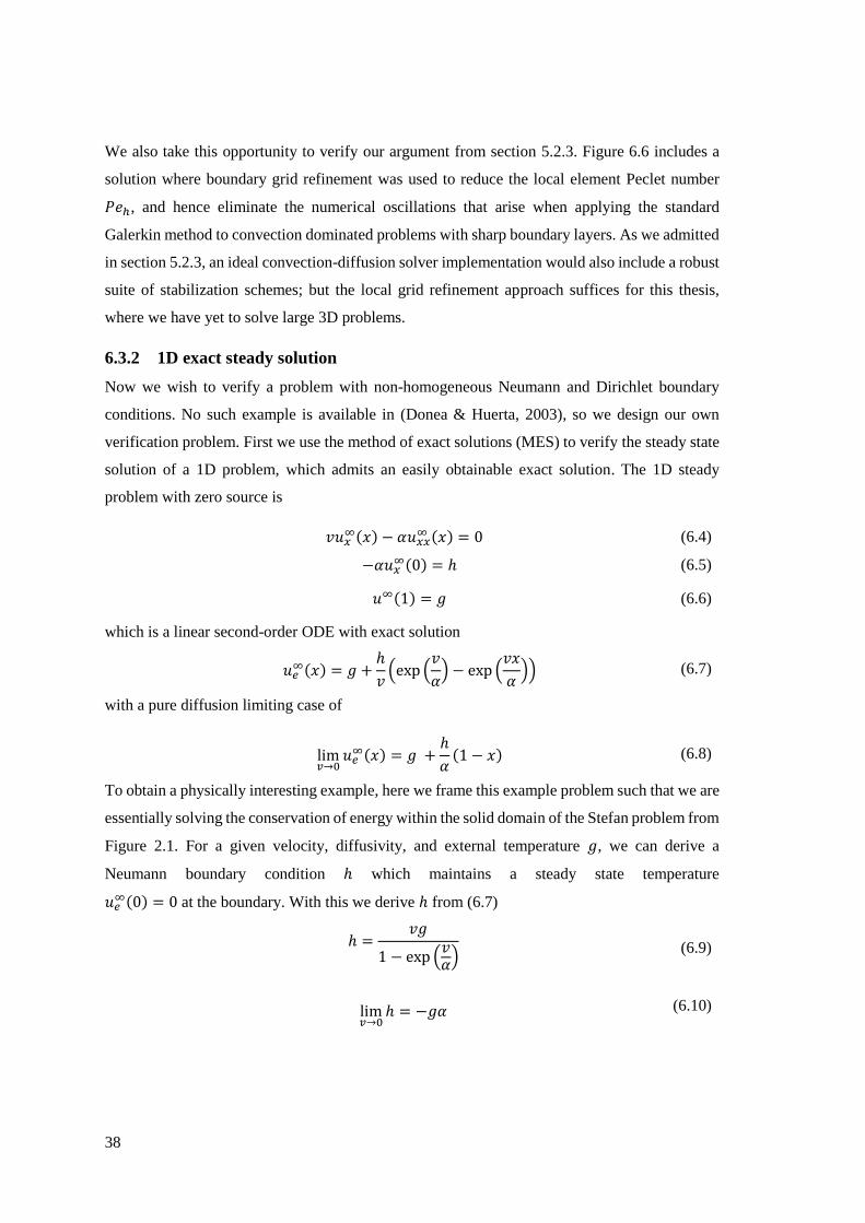
38
We also take this opportunity to verify our argument from section 5.2.3. Figure 6.6 includes a
solution where boundary grid refinement was used to reduce the local element Peclet number
𝑃𝑒ℎ, and hence eliminate the numerical oscillations that arise when applying the standard
Galerkin method to convection dominated problems with sharp boundary layers. As we admitted
in section 5.2.3, an ideal convection-diffusion solver implementation would also include a robust
suite of stabilization schemes; but the local grid refinement approach suffices for this thesis,
where we have yet to solve large 3D problems.
6.3.2 1D exact steady solution
Now we wish to verify a problem with non-homogeneous Neumann and Dirichlet boundary
conditions. No such example is available in (Donea & Huerta, 2003), so we design our own
verification problem. First we use the method of exact solutions (MES) to verify the steady state
solution of a 1D problem, which admits an easily obtainable exact solution. The 1D steady
problem with zero source is
𝑣𝑢𝑥∞(𝑥) − 𝛼𝑢𝑥𝑥
∞ (𝑥) = 0 (6.4)
−𝛼𝑢𝑥∞(0) = ℎ (6.5)
𝑢∞(1) = 𝑔 (6.6)
which is a linear second-order ODE with exact solution
𝑢𝑒∞(𝑥) = 𝑔 +
ℎ
𝑣(exp (
𝑣
𝛼) − exp (
𝑣𝑥
𝛼)) (6.7)
with a pure diffusion limiting case of
lim𝑣→0
𝑢𝑒∞(𝑥) = 𝑔 +
ℎ
𝛼(1 − 𝑥) (6.8)
To obtain a physically interesting example, here we frame this example problem such that we are
essentially solving the conservation of energy within the solid domain of the Stefan problem from
Figure 2.1. For a given velocity, diffusivity, and external temperature 𝑔, we can derive a
Neumann boundary condition ℎ which maintains a steady state temperature
𝑢𝑒∞(0) = 0 at the boundary. With this we derive ℎ from (6.7)
ℎ =𝑣𝑔
1 − exp (𝑣𝛼)
(6.9)
lim𝑣→0
ℎ = −𝑔𝛼 (6.10)

39
For this study, we will always use (6.9). The exact steady state defined by (6.4)-(6.9) is
𝑢𝑒∞(𝑥) = 𝑔
exp (𝑣𝑥𝛼) − 1
exp (𝑣𝛼) − 1
(6.11)
lim𝑣→0
𝑢𝑒∞(𝑥) = 𝑔𝑥 (6.12)
The exact steady state solutions shown in Figure 6.7 are for a variety of convection velocities,
diffusivities, Dirichlet boundary conditions, with the corresponding Neumann boundary
condition (6.9). Peclet was run in fully implicit mode, 𝜃 = 1, to produce approximately steady
state solutions which are not shown here, because they do not visually differ from the exact
solutions. The code produces the correct steady result; but in this thesis we will only present the
rigorous calculation of empirical orders of convergence for the unsteady problem, since this is
what Peclet actually solves.
These exact steady state solutions are useful for the design of our manufactured solutions in the
following sections. They provide a way for us to anchor our manufactured solutions to reality.
Figure 6.7: Exact 1D steady solutions of the convection-diffusion equation
A Dirichlet BC is set on the right, while the Neumann BC set on the left is exactly the value such
that it yields a steady state temperature of 𝑢 = 0 on the Neumann boundary, given by (6.9). Note
how the pure diffusion solutions are a straight line. Increasing the convection velocity increases
the curvature of the solution, which begins to develop a sharp boundary layer at the Neumann
boundary. Increasing the velocity to larger values forces the boundary layer even closer to the
edge, increasing its sharpness.

40
6.3.3 1D unsteady manufactured solution
The unsteady 1D problem is
𝑢𝑡(𝑥, 𝑡) + 𝑣𝑢𝑥(𝑥, 𝑡) − 𝛼𝑢𝑥𝑥(𝑥, 𝑡) = 𝑠(𝑥, 𝑡) ∀ (𝑥, 𝑡) ∈ [0,1] × (0,1] (6.13)
𝑢(𝑥, 0) = 𝑢0 (6.14)
−𝛼𝑢𝑥(0, 𝑡) = ℎ(𝑡) (6.15)
𝑢(1, 𝑡) = 𝑔 (6.16)
A closed form solution for the unsteady 1D problem (6.13)-(6.16) is not easily obtainable.
Therefore, this work employs the method of manufactured solutions (MMS) to verify the spatial
and temporal orders of convergence of the unsteady problem.
Generally, MMS does not require a solution design with any physical meaning. This property
can be useful for manufacturing solutions that cover a wide range of code capabilities in a small
number of coverage tests. For our present problem (6.13)-(6.16), it is easy enough to construct a
somewhat physically meaningful solution. We do this by making a small modification to the
exact solution of the steady solution 𝑢∞. We design an unsteady solution where the initial values
𝑢0 are equal to the cold temperature 𝑔. We use an exponential term to transition from 𝑢0 to 𝑢∞,
i.e.
𝑢0 = 𝑔 (6.17)
𝑢∞ = 𝑔exp (
𝑣𝑥𝛼 ) − 1
exp (𝑣𝛼) − 1
(6.18)
𝑢𝑀(𝑥, 𝑡) = 𝑢0 + (𝑢∞ − 𝑢0)(1 − exp(−𝛽𝑡2)) (6.19)
Altogether (6.17)-(6.19) yield
𝑢𝑀(𝑥, 𝑡) = 𝑔(1 + (exp (
𝑣𝑥𝛼 ) − 1
exp (𝑣𝛼) − 1
− 1) (1 − exp(−𝛽𝑡2))) (6.20)
lim𝑣→0
𝑢𝑀(𝑥, 𝑡) = −𝑔((exp(−𝛽𝑡2) − 1)(𝑥 − 1) − 1) (6.21)
where we choose a sufficient coefficient 𝛽 such that 𝑢𝑀(𝑡 = 1) ≈ lim𝑡→∞
𝑢𝑀. The steady solution
of (6.21) is equivalent to (6.11). Figure 6.8 shows the unsteady behavior.

41
Figure 6.8: Manufactured 1D unsteady solutions
These are solutions to (6.20) and (6.21). Parameters not shown are 𝛼 = 1, 𝑔 = −1,𝛽 = 10 .
Via MMS we derive the Neumann boundary condition ℎ𝑀(𝑡) and source 𝑠𝑀(𝑥, 𝑡) that together
produce 𝑢𝑀(𝑥, 𝑡). Rather than doing all of this by hand, the author employed MATLAB’s
Symbolic Toolbox. The script and output are in Appendix A.
Derive ℎ𝑀 from (6.15)
ℎ𝑀(𝑡) = −𝛼𝜕
𝜕𝑥𝑢𝑀(0, 𝑡) = 𝑣𝑔
exp(−𝛽𝑡2) − 1
exp (𝑣𝛼) − 1
(6.22)
lim𝑣→0
ℎ𝑀(𝑡) = 𝑔𝛼(exp(−𝛽𝑡2) − 1) (6.23)
Note that the steady (𝑡 → ∞) limit of (6.22) is indeed equivalent to (6.9).
Derive 𝑠𝑀 from (6.13)
𝑠𝑀 = 𝑢𝑡 + 𝑣𝑢𝑥 − 𝛼
𝜕2
𝜕𝑥2𝑢 = 2𝛽𝑔𝑡 exp(−𝛽𝑡2)(
exp (𝑣𝑥𝛼 ) − 1
exp(𝑣𝛼) − 1
− 1) (6.24)
lim𝑣→0
𝑠𝑀(𝑥, 𝑡) = 2𝛽𝑔𝑡 exp(−𝛽𝑡2) (𝑥 − 1) (6.25)
The steady state is consistent with the exact solution with zero source, so the manufactured source
term 𝑠𝑀 vanishes as 𝑡 → ∞. Given sufficient 𝛽, 𝑠𝑀(𝑡) is nearly zero at 𝑡 = 1. The Neumann
boundary condition ℎ𝑀 also approaches a steady state. Both of these propreties are shown in
Figure 6.9.

42
Figure 6.9: Derived auxiliary conditions for manufactured solution.
Left: Neumann boundary condition, 𝑔 = −1, Right: Source term, 𝑣 = −5, 𝛼 = 1, 𝑔 = −1
Spatial and temporal convergence studies were run for a variety of 𝛼, 𝑣, and 𝑔. Table 2 shows
the results. See Appendix A for one of these parameter input files to Peclet, for which only the
respective parameters must be changed to reproduce all results. The theoretical convergence
orders are 𝑝 = 2 and 𝑞 = 2, so this verification was successful in all cases. The best match
shown here are the three cases which match to four significant digits. It should be possible to
further refine any of these cases to increase the precision of the empirical convergence order.
v 𝛼 𝑔 𝑝 𝑞 �̃� 𝛼 �̃� 𝑝 𝑞
-5 2 -2 1.996 2.000 -1 1 -2 2.015 2.001
-5 2 -1 1.992 1.999 -1 1 -1 2.008 2.002
-5 1 -2 1.998 1.999 0 2 -2 N/A 2.001
-5 1 -1 1.997 1.999 0 2 -1 N/A 2.001
-1 2 -2 2.022 2.001 0 1 -2 N/A 2.000
-1 2 -1 2.008 2.002 0 1 -1 N/A 2.000 Table 2: MMS 1D spatial (𝑝) and temporal (𝑞) convergence table
6.3.4 2D unsteady manufactured solution
Next we verify a 2D case with a spatially variable convection velocity. Keeping with the theme
of manufacturing physically relevant solutions, let us consider the case of a plate melting through
a block of ice with a temperature differential which causes rotation about one of its endpoints.
At the point of rotation, the convection velocity is zero. The velocity increases linearly with y.
This problem is sketched in the left side of Figure 6.10.

43
Figure 6.10: Sketch of 2D MMS problem, and exact unsteady solution.
Left: Sketch of the problem domain, boundaries, and parameters. 𝒗 is the convection velocity.
ℎ are Neumann boundary conditions. 𝑔 is a Dirichlet boundary condition.
Right: Unsteady solution for 𝛼 = 1, 𝑣𝑚𝑎𝑥 = 5, 𝑔 = −1 given the manufactured source term.
Similar to the 1D manufactured solution, we will choose initial and steady states
𝑢0 = 𝑔 (6.26)
𝑢∞(𝑥, 𝑦) = 𝑔exp (
𝑣max𝑥𝑦𝛼
) − 1
exp (𝑣max𝑦𝛼
) − 1 (6.27)
and use the same exponential function of time to transition between them
𝑢𝑀(𝑥, 𝑡) = 𝑢0 + (𝑢∞ − 𝑢0)(1 − exp(−𝛽𝑡2))
= 𝑔(1 + (1 −exp(𝑣max𝑥𝑦/𝛼) − 1
exp(𝑣max𝑦/𝛼) − 1) (exp(−𝛽𝑡2) − 1))
(6.28)
The Neumann boundary conditions and source term are again derived per the strong form. There
are many more terms than for the 1D problem, so the equations are in Appendix A. Convergence
studies were again run for a variety of 𝛼, 𝑣max, and 𝑔, with the results shown in Table 3.
𝛼 𝒗max 𝒈 𝒑 𝒒 𝛼 𝒗max 𝒈 𝒑 𝒒
2 -5 -2 2.036 2.058 1 -5 -2 1.999 2.058
2 -5 -1 2.036 2.058 1 -5 -1 1.999 2.059
2 -1 -2 2.013 2.042 1 -1 -2 2.007 2.029
2 -1 -1 2.012 2.042 1 -1 -1 2.007 2.029 Table 3: 2D MMS convergence table.
The columns are diffusivity, max velocity, Dirichlet BC, spatial convergence order, and temporal
convergence order.
𝛀𝑺
ℎ = ℎ(𝑥)
𝑔
ℎ = 0 𝒗(𝑦) = (
𝑣max 𝑦0
)
𝑥
𝑦
Rotation
axis

44
7 A realistic phase-change model: Moving melt film
So far we have neglected the actual phase-change process within the ambient dynamics ℒ, which
physically requires some non-zero latent heat ℎ𝑚. Ultimately the successful prediction of melting
probe trajectories will require a model for ℒ which resolves both the contact melting/sublimation
on the contact surface 𝚪𝑐, shown in Figure 3.1, and the refreezing throughout the entire ambient
domain 𝛀. In future work, we hope to apply a realistic melting model throughout 𝛀, perhaps
being the enthalpy-porosity model which we briefly presented in 2.1.2. For the purposes of this
thesis, we take a smaller step by only modeling an aspect of the phase-change near 𝚪𝑐.
This chapter models the phase-change near 𝚪𝑐 by considering the Stefan problem, previously
formulated in section 2.1.1. We embed the Stefan problem micro-scale melt film boundary which
is fixed to the rigid body (RB) and therefore moving in the global reference frame.
This is the first known attempt to use the convection-diffusion equation to model the unsteady
evolution of the temperature field in the domain around a boundary characterized by the Stefan
problem. Ideally with a consistently chosen velocity 𝑣 of the phase-change interface (PCI), melt
film thickness 𝛿, and wall temperature 𝑇𝑤, the temperature near 𝚪𝑐 would remain steadily at the
melting temperature 𝑇𝑚. We should expect to see deviations in the 2D domain. Also we can study
the sensitivity of the temperature profile near 𝚪𝑐 in respect to all parameters.
7.1.1 Modeling the domain near a melt film boundary
To model the domain near 𝚪𝑐, consider a case where the rigid body (RB) moves with a constant
velocity 𝑣. Figure 7.1 shows a simplified rectangular domain that results if we zoom in to the
contact surface from Figure 3.1 and ignore curvature. Most of the boundaries 𝚪 in Figure 7.1 map
directly to boundaries in Figure 3.1. There are two additional boundaries. Cutting out this section
near the contact surface introduces a new boundary 𝚪𝒔 which slices through the original solid
domain. On 𝚪𝑠 we apply a homogeneous Neumann (i.e. adiabatic) boundary condition, enforcing
zero lateral heat conduction out of the domain. Note that the grid is fixed in this reference frame,
so the RB’s velocity appears as the opposite of the convection velocity 𝑣.
The domain described by Figure 7.1 is entirely solid on the interior. A PC occurs on 𝚪𝑐 and 𝚪𝑚.
On 𝚪𝑚 we set the temperature directly and ignore the physical details of the PC; but on 𝚪𝑐 we
apply a heat flux boundary condition based on the Stefan condition from (2.1), which physically
models the latent heat of melting ℎ𝑚. Rearranging the Stefan condition equation yields the heat
flux to be applied to the melt boundary for a given velocity and probe temperature
𝑞+(𝒙) = 𝑞−(𝒙) − 𝜌𝑆ℎ𝑚𝑣 = −𝑘𝐿𝑇𝑚 − 𝑇𝑤(𝒙)
𝛿(𝒙)− 𝜌𝑆ℎ𝑚𝑣 (7.1)

45
Note that this is a heat flux, while we are simulating the convection and diffusion of a temperature
field. Consider the state equation, given by the first law of thermodynamics
𝜌𝑐𝑝𝜕𝑇
𝜕𝑡− ∇ ∙ (𝑘∇𝑇) = �̇�𝑉 (7.2)
where �̇�𝑉 is the volumetric heat flux. Normalizing by 𝜌𝑐𝑝 yields the heat equation
𝜕𝑇
𝜕𝑡− ∇ ∙ (𝛼∇𝑇) =
�̇�𝑉𝜌𝑐𝑝
(7.3)
With this knowledge we obtain a function for the Neumann boundary values
ℎ(𝒙) =𝑞+(𝒙)
𝜌𝑆𝑐𝑝,𝑆 (7.4)
We must assume that we have some function to compute the film thickness 𝛿(𝒙) ≈ 𝒪(1) μm.
Accurately predicting the melt film thickness requires solving the micro-scale problem. Note that
(2.1) and therefore (7.1) is a one-dimensional model which we apply in the normal direction at
every point 𝒙 on 𝚪𝑐. We use the thermal properties of ice near its melting temperature, which are
𝑘𝑆 = 2.14 W
m K, 𝜌𝑆 = 917
kg
m3, 𝑐𝑝,𝑆 = 2110
J
kg K, ℎ𝑚 = 3.34 ∙ 106
J
kg
The thermal diffusivity is then
𝛼𝑆 =𝑘𝑆
𝜌𝑆𝑐𝑝,𝑆= 1.11 ∙ 10−6
m2
s
And finally we need the thermal conductivity of water near its freezing temperature
𝑘𝐿 = 0.5611W
m K
Indeed, for a given 𝑣, 𝛿, 𝑇𝑤, and therefore ℎ, the bubble of a steady melt interface forms. Figure
7.2 shows how the size of the “bubble” inside of the melt interface decreases as we apply a heat
flux approaching the one specified by the exact Stefan condition, which is labeled ℎ∗. With the
exact ℎ∗, the temperature near the wall only nearly reaches the melting temperature, and so there
is no 𝑇 = 𝑇𝑚 isoline. This is exactly the expected behavior. This means that the convection-
diffusion equation is indeed useful for modeling the temperature distribution within the solid
domain near the heating surface of a close-contact melting problem with a moving heat source.

46
Figure 7.1: Domain near close-contact melt film
𝐿 is a reference length. 𝒗 is the convection velocity. Boundary conditions are Dirichlet on 𝚪𝐷
and Neumann on 𝚪𝑁.
Figure 7.2: Steady-state melt temperature contour for the Stefan condition based 2D problem
This is Peclet output visualized with ParaView. White isolines mark the phase-change interface
(PCI). The boundaries are color-coded according to Figure 7.1. ℎ is the Neumann BC prescribed
on the contact surface. ℎ∗ is the exact Neumann BC corresponding to the Stefan condition.
7.1.2 Sensitivity of the melt film boundary
To analyze the sensitivity of the Stefan-condition based Neumann boundary to the parameters,
consider a 1D slice down the center of the domain from Figure 7.2. Here we initialize with the
known steady state solution for 𝑣∗, but evolve the unsteady convection-diffusion equation with
a perturbed velocity of 𝑣. Small perturbations on 𝑣 significantly change the steady state
temperature at the boundary. The same occurs for small perturbations in the wall temperature 𝑇𝑤
or melt film thickness 𝛿. The heat flux is very sensitive to the melt film thickness. Physically the
melt film thickness is dependent on the velocity and the wall temperature, which would have a
regulating effect if we were resolving the dynamics of the melt film itself.
In section 8.4.2 we will demonstrate a coupled problem where we perturb the heat flux and
simulate the dynamic response of the rigid body’s velocity. It would be interesting to instead
𝚪𝑚 ⊂ 𝚪𝐷
𝛀𝑺
𝚪𝑐 ⊂ 𝚪𝑁
𝚪𝑒 ⊂ 𝚪𝐷
𝚪𝒔 ⊂ 𝚪𝑁 𝑣
𝐿
ℎ = 2ℎ∗
ℎ = 1.2ℎ∗ ℎ = 1.1ℎ∗
𝑣
𝜴𝑺
(Snapshot from Figure 3.1)

47
control the wall temperature embedded in the Stefan condition. The sensitivity of the boundary
value to small changes in the parameters makes this impractical without a function to update the
melt film thickness, which regulates the heat flux and therefore the velocity. This makes intuitive
sense, since with the methods developed in this thesis, there is no means of resolving features on
the scale of the melt film thickness.
Figure 7.3: Sensitivity of the Stefan condition based Neumann boundary in 1D
The top-left visualizes large time steps reaching the steady state solution. The bottom-right
visualizes small time steps toward the beginning of the simulation, highlighting the unsteady
behavior. 𝑇 is the temperature. 𝑣 is the convection velocity. 𝑣∗ is the steady velocity
corresponding to the Stefan condition. 𝑣𝑚 is the velocity of the phase-change interface (PCI).
𝑣𝑚 ≈ 6𝑥𝑟𝑡𝑟
When holding the melt film
thickness and the heat flux constant,
a 1% velocity perturbation causes
the melt interface to move at the
velocity of six reference lengths 𝑥𝑟
per reference time 𝑡𝑟
Approximate
steady state is
reached at 𝑡 = 𝑡𝑟
Here the unsteady behavior
is highlighted

48
8 Coupling ℋ and ℒ: The complete forward problem
In the previous chapters, we have already presented mathematical models for the split operators
ℋ and ℒ, which are respectively the rigid body dynamics (RBD) operator and the ambient
dynamics operator. We further have already implemented these models and tested them
independently. In chapter 3, we briefly introduced the abstract mathematical formulation of the
coupled problem. For quick reference, we repeat here the coupled split operators
�̇�(𝑡) = ℋ൫𝑡, 𝝃(𝑡), 𝒖(𝑡, 𝒙)൯, 𝒖𝑡(𝑡, 𝒙) = ℒ(𝑡, 𝒖(𝑡, 𝒙), 𝝃(𝑡), �̇�(𝑡)) (8.1)
8.1 Temporal coupling
In chapter 4, we formulated ℋ as a minimization problem which requires the solution of a
constrained nonlinear program (4.9)-(4.12) at every time step. In chapter 5, we formulated ℒ as
an initial boundary value problem that requires the solution of a linear system (5.17) at every
time step. In chapter 3, we introduced how these two problems are coupled via the shared rigid
body (RB) state 𝝃 and ambient state 𝒖. As discussed in chapter 3, both 𝝃(𝑡) and 𝒖(𝑡) depend on
time 𝑡. We couple ℋ and ℒ by requiring that they share an equivalent 𝝃𝑖 = 𝝃(𝑡𝑖) and 𝒖𝒊 = 𝒖(𝑡𝑖)
at every discrete time 𝑡𝑖. In the current chapter, we detail the coupling procedure for (8.1). We
will write the algorithm for the iterative time evolution procedure, followed by a detailed
description of the software implementation, finally followed by results.
Different discrete time step sizes are appropriate for each operator. In general, the trajectory
integration ℋ allows for larger time steps. We view this as a multi-index into discrete time, as
visualized in Figure 8.1. We discretize each ℋ time interval 𝒕𝑖 onto a smaller scale for ℒ. When
discussing ℋ, we may use a single index for time interval 𝒕𝑖 and discrete time 𝑡𝑖. When
discussing ℒ, which includes the smaller time scale, we must use the multi-indexed time interval
𝒕𝑖,𝑗 and discrete time 𝑡𝑖,𝑗.
𝑖 = 0 𝑖 = ⋯ 𝑖 = 𝑚 − 1
𝑗 = 0 … 𝑗 = 𝑛 𝑗 = 0 … 𝑗 = 𝑛 𝑗 = 0 … 𝑗 = 𝑛
Figure 8.1: Multi-indexed time discretization for the split operators
The rigid body dynamics ℋ is split into 𝑚 time intervals. Within each 𝑖th interval, the ambient
dynamics ℒ are further split into 𝑛 time sub-intervals. Note that as time increases from left to
right along the axis �̂�, each time interval is closed on the left and open on the right, i.e. 𝒕 ={𝑡 ∈ ℝ: 𝑡𝑖 ≤ 𝑡 < 𝑡𝑖+1 }.
𝒕𝑖
𝒕𝑖,𝑗 𝑡𝑖,𝑗 𝑡0,0 𝑡𝑚−1,0
𝑡𝑖
�̂�

49
In the following equations, the superscripted 𝝃𝑖 denotes the rigid body state evaluated at time 𝑡𝑖,
and the superscripted 𝒖𝑖,𝑗 denotes the evaluation of the ambient state at time 𝑡𝑖,𝑗, i.e.
𝝃𝑖 = 𝝃( 𝑡𝑖) (8.2)
𝒖𝑖,𝑗(𝒙) = 𝑢൫𝒙, 𝑡𝑖,𝑗൯ (8.3)
Now we label the solutions for a discrete time step of ℋ or ℒ as the discrete operators 𝒽 or ℓ,
which respectively advance 𝝃 or 𝒖 a discrete time step, i.e.
𝝃𝑖+1 = 𝒽൫𝒖𝑖 , 𝝃𝑖൯, 𝒖𝑖,𝑗+1 = ℓ൫𝑡𝑖,𝑗+1 − 𝑡𝑖,𝑗, 𝒖𝑖,𝑗, 𝝃𝑖 , �̇�𝑖൯ (8.4)
Evolving the coupled problem in time, and hence obtaining the time evolution both of 𝝃(𝑡) and
𝒖(𝑡) , requires an iterative procedure explained by Algorithm 1. To help explain the examples in
this chapter, we also show here the time-dependent heat flux input ℎ𝑖. There is one additional
complication shown in the algorithm: We superpose the velocity �̇� when solving ℋ and ℒ, so we
must track an additional state in order to view the rigid body from a global reference frame. We
name this auxiliary state 𝝃𝑉.
1. 𝝃0 ≔ 𝝃, �̇�0 ≔ �̇�
2. 𝝃𝑉0 ≔ 𝝃0
3. for 𝑖 ∈ [0,1,2, … ,𝑚):
a. for 𝑗 ∈ [0,1,2,… , 𝑛):
i. 𝒖𝑖,𝑗+1 ≔ ℓ൫𝒕𝑖,𝑗, 𝒖𝑖,𝑗, 𝝃𝑖 , �̇�𝑖; ℎ𝑖൯
b. 𝒖𝑖+1,0 ≔ 𝒖𝑖,𝑛
c. 𝝃𝑖+1 ≔ 𝒽൫𝒖𝑖+1,0, 𝝃𝑖൯
d. �̇�𝑖+1 ≔ �̇�𝑖 + ൫𝝃𝑖+1 − 𝝃𝑖 ൯/𝒕𝑖
e. 𝝃𝑉𝑖+1 ≔ 𝝃𝑉
𝒊 + ൫𝝃𝑖+1 − 𝝃𝑖 ൯ + 𝒕𝑖 �̇�𝑖
Algorithm 1: Iterating the coupled problem through time
Line 1.a.i. of Algorithm 1 shows that the previous ambient state is used to initialize ℓ, so that the
ambient state is evolving in time through all steps of the trajectory. The phase-change interface
(PCI) is a feature of 𝒖(𝑡) and hence is also evolving in time. Recall that the convection velocity
profile 𝒗(𝒙) within ℒ is derived from the state time derivative �̇�. For a sufficiently high heat flux
ℎ and sufficiently low velocity 𝒗, the PCI moves away from the rigid body. This behavior is
shown in Figure 7.2. In such cases, solving 𝒽 yields an update to 𝝃. Dividing the difference of
the updated state 𝝃𝑖+1 and the previous state 𝝃𝑖 by the length of the time interval 𝒕𝑖 yields an
update for �̇�. For constant ℎ, iterating 𝑖 converges �̇� toward a steady state.
Set initial values for the rigid body (RB) state and its derivative.
At the initial RB state, the global auxiliary RB state is equivalent.
Loop through the discrete rigid body dynamics (RBD) time steps.
Loop through ambient dynamics time steps.
Solve an ambient dynamics step.
Solve a RBD time step.
Set the correct index per Figure 8.1.
Update the state time derivative.
Update the global auxiliary state.

50
Here a fundamental limitation of the superposed velocity concept can be seen. When the velocity
is too high or the heat flux is too low, no PCI will form, and hence ℋ cannot update the position,
and Algorithm 1 cannot update the velocity. This means that the heat flux input ℎ must be non-
decreasing, i.e. the rigid body cannot slow down.
In this work, Algorithm 1 was implemented in Python and C++. In addition to the algorithm, the
implementation requires pre-processing, post-processing, and an interface between the Python
driver and the C++ implementation of ℒ. Recall from chapters 5 and 6 that ℒ is a partial-
differential equation (PDE), which is assembled as a linear system and solved by the finite
element library deal.II (Bangerth, Davydov, & Heister, 2016). It is not trivial to use an existing
solution to initialize the PDE solver in Line 1.a.i. of Algorithm 1. We explain these difficulties
in section 8.3.
8.2 The overall trajectory simulator software system
For this work, Algorithm 1 was implemented in Python and C++. The primary components of
the implementation, and how they interact, are shown in Figure 8.2.
Figure 8.2 shows the overall flow of the trajectory simulator, how it interfaces with the PDE
solver, and how the PDE solver re-initializes based on input from the simulator. The entire source
code is shared at a public GitHub repository (Zimmerman, dimice-python-cpp, 2016). Note that
this repository includes the PDE solver as a submodule. While we presented the most recent and
complete version of the PDE solver, Peclet, in chapter 6, the submodule points to an older version
that is named dimice-pde-dealii.
Python (using scipy, matplotlib, and vtk) C++ (using deal.II and boost)
H: Minimize Energy Function
L: Solve PDE
u: Ambient State
ξ: RB state Transformed
Gridu0: Initial
Values
Generate Grid
Read and Interpolate
RB Geom.
Interpolant Write data
Extrapolated FE Field Function
Visualize
Data Process File
Solution
Image
Restart Files
Figure 8.2: Software system overview for coupled ℋ and ℒ.
ℋ determines the rigid body dynamics (RBD), while ℒ determines the ambient dynamics. The
components outlined in bold map directly to steps in Algorithm 1. The majority of the
components are for pre-processing, post-processing, and implementation details.
All time steps output by the PDE solver are archived so that they can be explored in ParaView
(Kitware, 2016). The final solution for each trajectory time step is read by VTK and interpolated
with SciPy (The Scipy community, 2016). matplotlib (Hunter, Dale, Firing, & Droettboom,

51
2016) is used to visualize the state of the rigid body (RB) and the phase-change interface (PCI).
Additionally, a contour is drawn where the ambient temperature is 80% of the farfield
temperature, to get a sense for the time evolution of the ambient away from the PCI.
The Python program is decomposed into a group of modules shown in Figure 4.4. The object-
oriented design of this program is flexible, making it simple to test new ideas. The main class is
Trajectory, which has instances of the Body and PDE classes as members. With this
framework, the user imports the trajectory module, instantiates a Trajectory object in their
own script, and modifies the parameters that are members of their instance before finally running
the trajectory with the Trajectory.run_steps or Trajectory.run_step method. The
entire user script for generating Figure 8.8 is provided in Appendix A. After iterating the method
Trajectory.run for half of the total time steps, the Neumann boundary condition was
increased, and the method Trajectory.run was iterated again for the remaining time steps. The
state is always saved within the Trajectory instance, making it simple to generate trajectory
simulations with a sequence of different inputs.
As detailed in section 4.3.2, SciPy’s SLSQP routine within scipy.minimize (The Scipy
community, 2016) was used to solve the minimization problem. SciPy is a widely used library
for scientific computing; and it is convenient to try this as a first approach. In future work when
extending to 3D and more complex ambient dynamics models, it will likely become necessary to
use interior point optimization instead. A third-party Python interface, pyipopt, does exist for
ipopt, but it does not appear to be actively supported.
8.3 Implementation of the interface to ℒ in deal.II
Three capabilities were needed which extend the PDE solver:
Transform a grid according to a state vector
Write and read an entire finite element solution to and from the hard drive
Initialize a solution based on interpolation and extrapolation of an old solution
Figure 8.3 visualizes why interpolation and extrapolation are necessary. Reading and writing to
and from the disk is necessary so that the external driver, the trajectory simulator, can run the
PDE solver from the command line, and restart each execution based on the solution from the
previous step. The details of implementing each of these three features in deal.II presents some
difficulties, especially with reading solutions from the hard drive. In the next sections, we will
discuss some of the more interesting points.

52
Figure 8.3: Sketch of grid transformation and initial values interpolation/extrapolation
The liquid domain is colored red and the solid domain is colored blue. The minimum energy state
of the rigid body (RB) for the given ambient is colored green. The outline of the transformed grid
corresponding to the new RB state is shown on the right-hand sketch, which illustrates regions
of the PDE solution which must be interpolated or extrapolated.
8.3.1 Grid transformation
The rigid body (RB) transformation can be applied either absolutely from the original RB
position, or relatively at each sequential RB position. For RB transformations either should
suffice; but the absolute approach is simpler. The next question is whether to solve the ambient
dynamics numerically on the reference grid or on the transformed grid. Either approach will
require multiplying the entire grid by the transformation matrix. During pre-processing either the
current grid must be transformed to conform with the reference grid, or vice versa.
A careful read of the deal.II documentation leaves us with only one option that will work for
parallel computations. In the detailed description of GridTools::Transform, the deal.II
developers say that transforming a refined parallel (distributed) Triangulation will result in
invalid ghost cells, which breaks many methods, e.g. the Kelly error estimator which is needed
for adaptive grid refinement. Therefore, we will only transform the coarse grid, and not solutions
which are always on refined grids.
8.3.2 Interpolation and extrapolation
Initializing the solution values based on a previous solution is a difficult task, because the grid
has moved. Essentially the previous solution must be interpolated onto a transformation of the
previous grid. There are at least three ways one could attempt to do this, in decreasing order of
the fidelity of the projection:
1. Create a field function that uses all of the finite element discretization and solution
information
Solid Liquid Minimum energy state
of rigid body (RB)
Transformed grid Extrapolation
Required

53
2. Use VTK methods to sample VTK solution files
3. Treat the nodal data as a scattered set and use a scattered data interpolation algorithm
The first option is ideal. Thankfully deal.II has a built-in function that is almost what we need,
except for a major drawback. Given a finite element discretization and solution, one can create a
FEFieldFunction, which represents the finite element solution that can be continuously
sampled within the domain. The key drawback here is that the sample must be within the domain,
which is not good enough for us, since we wish to move the grid. Already for the simple geometry
in Figure 8.3, we see four regions where data must be sampled from outside of the domain of the
existing finite element solution.
In this work, FEFieldFunction was extended with exception handling that performs nearest-
neighbor extrapolation. For the outer domain, nearest-neighbor is fine, since in our ambient
dynamics model ℒ we specify a constant environment temperature 𝑇𝑒 which is normally used as
a Dirichlet boundary condition 𝑔. On the other hand, near the heat source surface, nearest-
neighbor extrapolation is inaccurate. Fortunately, extrapolation only occurs aftward of the
movement, and we are particularly interested in the forward region driving the movement. Figure
8.4 shows how, even for a reasonably coarse grid, the majority of the melt interface does not
move during the interpolation procedure. There is an obvious error highlighted in red, far aft of
the body, where the grid is coarsest. This is acceptable for our problem.
Regarding the detailed implementation, a new class was designed which contains a
FEFieldFunction member, along with a routine to extrapolate to the nearest boundary after
catching the proper exception. The entire class only required 84 lines of code, including the crude
custom routine for finding the nearest boundary vertex. The entire source code is at
peclet/source/extrapolated_field.h (Zimmerman, Peclet, 2016). A slightly
abbreviated version is in Appendix B.
In theory, the second option, interpolating the field as a set of scattered data points, should be
simple and worth trying. Unfortunately, libraries that support the interpolation of scattered data
are not widely available. MATLAB’s ScatteredInterpolant, a relatively new feature,
supports n-dimensional natural neighbor interpolation. The natural neighbor method is the only
known option for smoothly interpolating unstructured finite element solutions, where we use the
strict definition of “interpolate”, meaning that the interpolant must exactly match the data where
data is given. The best available option in Python is SciPy’s LinearNDInterpolator,
which, as the name implies, only currently supports linear (i.e. non-smooth, only 𝐶0 continuous)
interpolation. No options have been found in C/C++ for general scattered data interpolation.

54
Figure 8.4: Error from interpolating onto a transformed grid
𝑇𝑚 is the melting temperature of the phase-change material (PCM). The error is most evident in
the regions with a coarse mesh.
8.3.3 Restarting onto a transformed grid with a finite element field function
Developing the capability to write and read the entire finite element solution, rather than a simple
projection of it for a visualization tool, to and from the file system was substantially more difficult
than expected. The technique is not clearly defined in the deal.II documentation, and the problem
becomes much more difficult when using parallel distributed triangulations.
The idea employed in this work is to serialize, using the boost library (Dawes & Abrahams,
2016), all data needed to construct the FEFieldFunction that samples the solution. When
restarting the PDE solver, the data is deserialized, the FEFieldFunction is constructed, and
this Function is passed as an argument to the initial values function. In Peclet, the methods to
write and read this data are encapsulated in the source file
peclet/source/fe_field_tools.h (Zimmerman, Peclet, 2016).
8.3.4 Sampling the finite element solution outside of the solver
As shown in Figure 8.2, we simulate the coupled trajectory with a Python driver. Since the
minimization problem ℋ is solved within Python, we need to share a representation of the finite
element solution outside of the PDE solver, which is a compiled C++ program. This will allow
us to sample the temperature field for evaluating the inequality constraints (4.5). The finite
element solution resides in a complex data structure that is not easily shared externally. A typical
solution output file, e.g. one formatted for a visualization tool, omits information about the basis
used to construct the solution, and also omits information about geometric manifold, i.e. most
visualization tools assume linear interpolation between all nodes.
𝑇 = 𝑇𝑚 contour from original solution
𝑇 = 𝑇𝑚 contour from
solution interpolated onto
transformed grid

55
There are three primary ways we could sample the solution output. In order of decreasing
complexity:
A. Program an interface that uses the internal data structure. This would require 1. using a
library such as pybind to create Python bindings for the C++ code, and 2. compiling a
shared library. Neither of these tasks are trivial.
B. Interface with the visualization library to benefit from the discretization structure. This
would require 1. constructing an object that represents the geometry we wish to sample
onto (the hull of the body), 2. reading the VTK solution, and 3. applying a
VTKProbeFilter with the VTK solution as the data source, and the geometry as a
sampling input.
C. Construct an interpolator based on a scattered interpretation of the output data. This
would require 1. reading the solution as a set of unstructured data points, 2. constructing
an interpolator using either linear or natural neighbor interpolation
Option A was briefly attempted, but not yet with any success. Option B was attempted with more
effort, but working directly with VTK has proven difficult. Instead scripting ParaView (Kitware,
2016) with Python might be a good approach to try in the future. Option C has been successful
and is what we use in this chapter. The scattered data representation has already been shown to
work in the MATLAB example from section 4.3.3, and a scattered data interpolation class exists
in SciPy.
SciPy provides the LinearNDInterpolator class to interpolate scattered data. MATLAB’s
ScatteredInterpolant class is more advanced, e.g. it supports a natural neighbor
interpolation which is once differentiable, but SciPy’s routine was sufficient for this work.
Figure 8.5: Scattered data interpolation with SciPy LinearNDInterpolator.
The circles mark nodal values from the VTK solution output file. The domain is shaded with bi-
linear interpolation. Since the data is considered scattered, values are interpolated inside of the
rigid body (RB) surface boundary as well.

56
8.4 Example results for the coupled trajectory
The coupled problem is implemented in such a way that trajectory simulations can be run for a
variety of geometries and boundary conditions, with or without coupling the rigid body’s velocity
as the convection velocity. First in this section we show three examples where only the position
has been coupled for a 2D sphere-cylinder geometry, and then we show an example where the
velocity has been coupled for a circular geometry.
8.4.1 Coupled position
Turning trajectories for different parametric geometries are shown in Figure 8.6. Here the
temperature of the heat source surface was prescribed, rather than a heat flux. Asymmetric
temperatures were applied to the nose of a 2D sphere-cylinder.
Figure 8.6: Example trajectories with coupled position
Top: Large ratio of aft-body length to nose radius. Bottom: Small ratio of aft-body length to nose
radius. Time is stepping from left to right. The rigid body (RB) surface at the current time step is
drawn in red, while the RB from the previous time step is drawn with a dashed yellow line. A
blue isoline marks the phase-change interface (PCI) in each plot, while a black isoline marks
where the temperature is 80% of the environment temperature, to illustrate the time evolution of
the entire ambient. Warm Dirichlet BC’s have been applied to the body, except for a hot BC on
one side of the nose to cause a turn.
Rigid body (RB) Phase-change
interface (PCI)

57
To generate Figure 8.7, rather than setting the body’s temperature as a Dirichlet BC, the heat flux
out of the body was set as a Neumann BC. A larger value was set at the nose, so the melt forms
near the nose before the aft-body. In our current implementation of ℋ, the optimization problem
must be initialized with a feasible state. The constraints 𝒈 require that the temperature is strictly
greater than the melting temperature, so the state of the RB is invalid until melt has formed around
the entire RB, effectively restricting the RB’s movement. As soon as the optimizer begins with a
feasible state, it is free to minimize the problem, which for our examples in this work is simply
minimizing gravitational potential (as detailed in section 4.2). This leads to a very large amount
of movement in a single time step of the coupled problem.
Figure 8.7: Example of restricted movement when the rigid body is not surrounded by liquid
A larger heat flux was prescribed on the nose than the aft-body, and so the melt forms around the
nose before forming around the rest of the body. Time is stepping from left to right. The rigid
body (RB) surface at the current time step is drawn in red, while the RB from the previous time
step is drawn with a dashed yellow line. A blue isoline marks the phase-change interface (PCI)
in each plot, while a black isoline marks where the temperature is 80% of the environment
temperature, to illustrate the time evolution of the entire ambient. The body is restricted from
movement until it is entirely surrounded by melt, and is first permitted to move in step seven.
A gap has formed, but movement
is restricted until the entire RB is
surrounded by liquid Phase-change
interface (PCI)
Rigid body (RB)

58
8.4.2 Coupled velocity and position
To explore the behavior when coupling the convection velocity to the velocity of the rigid body
(RB), we consider a circular geometry with a spatially constant Neumann BC ℎ(𝑡) applied on
the heat source surface 𝚪ℎ, and with a scalar convection velocity 𝑣 pointing upward. For some
initial velocity 𝑣0 and a constant heat flux in time ℎ that is sufficiently high to form a melt, an
iteration of ℋ in Algorithm 1 moves the RB and increases the velocity 𝑣. The next PDE solution
will in turn have reduced temperatures near 𝚪ℎ, which then reduces the size of the position and
velocity update in the next iteration of ℋ. This eventually reaches a steady state, where no gap
forms between 𝚪ℎ and the PCI, and hence an iteration of ℋ does not yield any RB state update.
To produce the result in Figure 8.8, after an approximately steady state velocity was reached, the
heat flux ℎ was increased by 20%. As we would expect, this causes a dynamic response in the
velocity, which eventually reaches a new steady state.
The right side of Figure 8.8 verifies the expected linear relationship between the heat flux and
the steady state velocity. This qualitative result is promising. For the method of this thesis to
quantitatively predict such a trajectory, the ambient dynamics model ℒ must be either augmented
or replaced to account for the latent heat of melting ℎ𝑚. With a model accounting for ℎ𝑚, we
would expect the same steady state velocities as shown here, but different unsteady behavior.
Figure 8.8: Example of coupled velocity with circular geometry
Left: Annotated PDE solution at time 𝑡 = 0.25 𝑡𝑓, viewed in ParaView.
Right: Dynamic response of velocity given a step function (in time) for the heat flux input. 𝑣 is
the velocity and ℎ is the heat flux. The Python script to generate this result is in Appendix A.
ℎ applied to entire surface
Phase-change
interface (PCI)
𝑣
Steady velocity
𝑡/𝑡max
𝑣/𝑣max
ℎ/ℎ
max

59
9 Summary, conclusions and proposals for future work
In meeting its primary goals, this thesis has
formulated a mathematical model for the general problem of rigid body heat source
trajectories through phase-change materials. We split the rigid body dynamics and the
ambient dynamic into two operators and the coupling of these operators.
formulated and implemented concrete examples of each of the two operators.
verified the correctness, and the spatial and temporal orders of accuracy, of our finite
element method (FEM) implementation for the ambient dynamics.
implemented the coupled problem with Python and C++.
demonstrated the coupled problem by showing the dynamic velocity response to a rapid
change in the heat flux, which causes the velocity to approach a new steady state. The
result verifies the expected linear relationship between the applied heat flux and the
steady state velocity.
Further, this thesis has shown that
interior-point optimization and sequential least-squares quadratic programming
(SLSQP) are both suitable for solving the presented minimization problem when
sampling a FEM solution for constraints. Interior-point optimization will likely be
superior for larger problems.
the convection-diffusion equation can model the temperature distribution within the
solid domain near the close-contact melting interface of a heat source moving through a
phase-change material. This is accomplished by representing the micro-scale melt film
attached to the heating surface as a Neumann boundary, with a value based on the heat
flux specified by the Stefan condition.
the Stefan condition based Neumann boundary condition is super-sensitive to changes
in the wall temperature, the micro-scale melt film thickness, and the velocity of the
melting interface. This suggests that this phase-change model might not be useful for
predicting the unsteady physical behavior. This motivates the future work of
implementing a realistic melting model within the ambient domain.
convection dominated problems with sharp boundary layers can be solved with the
standard Galerkin formulation of the finite element method. Generally, this can be
handled with stabilization schemes that exactly compensate for the artificial loss of
diffusion when discretizing the convection operator. We demonstrated the option to
instead locally refine the grid at the boundary layer, effectively reducing the local
element Peclet number. We admit that this could be prohibitively expensive for large
3D problems.

60
Moving forward, we should first and foremost quantify the errors introduced by the operator
splitting. Error sources include the truncation error from time discretization, and
interpolation/extrapolation errors when transferring solutions to transformed grids.
The next critical step is to implement a realistic melting model. This will allow validation against
experimental trajectories. Also important, this will yield new geometric properties in the melt
interface, and hence qualitatively change the constraints of the minimization problem which
models the rigid body dynamics. We must verify that interior point optimization can robustly
handle these constraints.
Before attempting any larger problems, another important step is to optimize the routine for
interpolating and extrapolating the ambient field onto transformed girds. The critical issue is
efficient and accurate extrapolation.
Altogether the approach of this work shows promise and warrants further investigation. A key
decision point will be whether to continue with the transformed grid and interpolation approach
for the ambient dynamics, or to invent a new approach which does not require
interpolation/extrapolation. If such a new approach is found for the ambient dynamics, then the
rigid body dynamics formulation and the temporal coupling from this thesis should be equally
applicable.

61
Bibliography
Alexiades, V., & Solomon, A. D. (1993). Mathematical Modeling of Melting and Freezing
Processes. Washington; Philadelphia; London: Hemisphere Publishing Corporation.
Bangerth, W. (2016, July 25). Boundary conditions. Retrieved from Video Lectures, MATH 676,
Texas A&M University: http://www.math.tamu.edu/~bangerth/videos.676.21.65.html
Bangerth, W. (2016, April 16). Tutorial 26. Retrieved from deal.II:
http://www.dealii.org/8.4.1/doxygen/deal.II/step_26.html
Bangerth, W., Davydov, D., & Heister, T. (2016). The deal.II Library, Version 8.4. Journal of
Numerical Mathematics.
Belhamadia, Y., Kane, A. S., & Fortin, A. (2012). An enhanced mathematical model for phase
change problems with natural convection. International Journal of Numerical Analysis
and Modeling, 192-206.
Biegler, L. T. (2010). Nonlinear Programming. Philadelphia, PA: Society for Industrial and
Applied Mathematics and the Mathematical Optimization Society.
Brooks, A. N., & Hughes, T. J. (1982). Streamline upwind/Petrov-Galerkin formulatoins for
convection-dominated flows with particular emphasis on the incompressible Navier-
Stokes equations. Computer Methods in Applied Mechanics and Engineering, 199-259.
Cmglee. (2016, October). Retrieved from Wikimedia Commons:
https://upload.wikimedia.org/wikipedia/commons/thumb/3/33/Phase_diagram_of_wate
r_simplified.svg/512px-Phase_diagram_of_water_simplified.svg.png
COIN-OR. (2016, August). Ipopt. Retrieved from coin-or.org: https://projects.coin-or.org/Ipopt
Crank, J., & Nicolson, P. (1996). A practical method for numerical evaluation of solutions of
partial differential equations of the heat-conduction type. Advances in Computational
Mathematics, 6(1), 207-226.
Dachwald, B., Mikucki, J., Tulaczyk, S., Digel, I., Espe, C., Feldmann, M., . . . Xu, C. (2014).
IceMole: a maneuverable probe for clean in situ analysis and sampling of subsurface ice
and subglacial aquatic ecosystems. Annals of Glaciology, 14-22.
Dawes, B., & Abrahams, D. (2016, May 13). Retrieved from boost C++ Libraries:
http://www.boost.org/
Donea, J., & Huerta, A. (2003). Finite Element Methods for Flow Problems. Wiley.

62
Hsu, H.-W., Postberg, F., & al., e. (2015). Ongoing hydrothermal activities within Enceladus.
Nature, 207-210.
Hunter, J., Dale, D., Firing, E., & Droettboom, M. (2016, September 20). Retrieved from
matplotlib: http://matplotlib.org/
Kelly, D. W., De S. R. Gago, J. P., Zienkiewicz, O. C., & Babuska, I. (1983). A posteriori error
analysis and adaptive processes in the finite element method: Part I--Error Analysis.
International Journal of Numerical Methods in Engineering, 1593-1619.
Kitware. (2016, November). Retrieved from ParaView: http://www.paraview.org/
Kraft, D. (1988). A software pakcage for sequential quadratic programming. Köln: Institute for
Flight Mechanics, DLR German Aerospace Center.
Schüller, K. (2015). Development of a finite element model to describe the dynamic behavior of
the maneuverable ice exploration probe IceMole. Aachen, Germany: FH Aachen
University of Applied Sciences.
Schüller, K. (n.d.). CoMeTFoam.
Schüller, K., Kowalski, J., & Raback, P. (2016). Curvilinear melting -- A preliminary
experimental and numerical study. Internatoinal Journal of Heat and Mass Transfer,
884-892.
The Scipy community. (2016, September 19). scipy.optimize.minimize. Retrieved from scipy.org:
https://docs.scipy.org/doc/scipy-
0.18.1/reference/generated/scipy.optimize.minimize.html
Wächter, A., & Biegler, L. T. (2006, November). On the Implementation of a Primal-Dual
Interior Point Filter Line Search Algorithm for Large-Scale Nonlinear Programming.
Mathematical Programming, 25-57. Retrieved from COIN | OR: https://projects.coin-
or.org/Ipopt
Zimmerman, A. G. (2016, November 25). dimice-python-cpp. Retrieved from GitHub:
https://github.com/alexanderzimmerman/dimice-python-cpp/releases/tag/v0.2x-thesis-
pre
Zimmerman, A. G. (2016, June 27). dimice-trajectory-matlab. Retrieved from GitHub:
https://github.com/alexanderzimmerman/dimice-trajectory-matlab/releases/tag/v0.1x-
thesis-pre
Zimmerman, A. G. (2016, November 5). Peclet. Retrieved from GitHub:
https://github.com/alexanderzimmerman/peclet/releases/tag/v0.2x-thesis-pre

63
Appendix
A. Peclet code verification
Peclet parameter input file to reproduce Donea & Huerta Figure 5.17 with 𝑃𝑒(ℎ = 0.1) = 0.5
subsection meta
set dim = 1
end
subsection output
set write_solution_table = true
end
subsection pde
subsection parsed_velocity_function
set Function expression = 1.
end
subsection parsed_diffusivity_function
set Function expression = 0.1
end
subsection parsed_source_function
set Function expression = 1.
end
end
subsection initial_values
subsection parsed_function
set Function expression = 0.
end
end
subsection boundary_conditions
set implementation_types = strong, strong
subsection parsed_function
set Function expression = 0.
end
end
subsection refinement
set initial_global_cycles = 3
end
subsection time
set end_time = 1.2
set step_size = 0.01
end
Set to 0.01 to run for 𝑃𝑒 = 5
Edit this section to reproduce boundary refined case

64
Symbolic derivation of 1D MMS auxiliary conditions in MATLAB
syms x t g v alpha beta real syms ue(x) ue_v0(x) um(x,t) um_v0(x) syms sm(x,t) sm_v0(x,t) hm(t) hm_v0(t) ue = g*(exp(v*x/alpha) - 1)/(exp(v/alpha) - 1); ue_v0 = limit(ue, v, 0); um = g*(1 + ((exp(v*x/alpha) - 1)/(exp(v/alpha) - 1) - 1)*... (1 - exp(-beta*t^2))); um_v0 = limit(um, v, 0); umx = diff(um, x); hm = subs(-alpha*umx, x, 0); hm_v0 = limit(hm, v, 0); umt = diff(um, t); umxx = diff(umx, x); sm = umt + v*umx - alpha*umxx; sm_v0 = limit(sm, v, 0);
Symbolic derivation of 2D MMS auxiliary conditions in MATLAB
syms x y t g alpha beta vmax real syms vx(y) u0 uinfty(x,y) u(x,y,t) syms h_y0(x,t) h_x0(y,t) h_x1(y,t), s(x,y,t) vx = vmax*y; u0 = g; uinfty = g*(exp(vx*x/alpha) - 1)/(exp(vx/alpha) - 1); u = u0 + (uinfty - u0)*(1 - exp(-beta*t^2)); u = simplify(u); u_y0 = limit(u, y, 0); h_x0 = -alpha*diff(u, x); h_x0 = subs(h_x0, x, 0); h_y0 = -alpha*diff(u, y); h_y0 = limit(h_y0, y, 0); h_y1 = alpha*diff(u, y); h_y1 = subs(h_y1, y, 1); s = diff(u, t) + vx*diff(u, x) - ... alpha*(diff(diff(u, x), x) + diff(diff(u, y), y)); s_y0 = limit(s, y, 0);

65
Example Peclet parameter input file for 1D MMS
subsection meta
set dim = 1
end
subsection geometry
set grid_name = hyper_cube
set sizes = 0., 1.
End
subsection verification
set enabled = true
set exact_solution_function_name = parsed
subsection parsed_exact_solution_function
set Function constants = alpha=2, v=-5, g=-2, beta=10
set Function expression = -g*(((exp((v*x)/alpha) - 1)/
(exp(v/alpha) - 1) - 1)*(exp(-beta*t^2) - 1) - 1)
end end
subsection parsed_velocity_function
set Function constants = v=-5
set Function expression = v
end
subsection parsed_diffusivity_function
set Function constants = alpha=2
set Function expression = alpha
end
subsection parsed_source_function
set Function constants = alpha=2, v=-5, g=-2, beta=10
set Function expression = 2*beta*g*t*exp(-beta*t^2)*((exp((v*x)/alpha) -
1)/(exp(v/alpha) - 1) - 1)
end
subsection initial_values
subsection parsed_function
set Function expression = -2*1.000000001
end
end
subsection boundary_conditions
set implementation_types = natural, strong
set function_names = parsed, constant
set function_double_arguments = -2.
subsection parsed_function
set Function constants = alpha=2, v=-5, g=-2, beta=10
set Function expression=(g*v*(exp(-beta*t^2) - 1))/
(exp(v/alpha) - 1)
end
end
subsection refinement
set initial_global_cycles = 6
end
subsection time
set global_refinement_levels = 6
end

66
Example Peclet parameter input file for 2D MMS
subsection meta
set dim = 2
end
subsection geometry
set grid_name = hyper_rectangle
set sizes = 0., 0., 1., 1.
end
subsection verification
set enabled = true
subsection parsed_exact_solution_function
set Function constants = epsilon=1.e-14, alpha=2, vmax=-5, g=-2, beta=10
set Function expression = if(y < epsilon,g + (g - g*x)*(exp(-beta*t^2) - 1),
g + (g - (g*(exp((vmax*x*y)/alpha) - 1))/(exp((vmax*y)/alpha) - 1))*
(exp(-beta*t^2) - 1))
end
end
subsection parsed_velocity_function
set Function constants = vmax=-5
set Function expression = vmax*y; 0
end
subsection parsed_diffusivity_function
set Function constants = alpha=2
set Function expression = alpha
end
subsection parsed_source_function
set Function constants = epsilon=1.e-14, alpha=2, vmax=-5, g=-2, beta=10
set Function expression = if(y<epsilon,(g*exp(-beta*t^2)*(x - 1)*(2*vmax^2*x^2 - vmax^2*x -
2*vmax^2*x^2*exp(beta*t^2) + 12*alpha*beta*t + vmax^2*x*exp(beta*t^2)))/(6*alpha),- alpha*((exp(-
beta*t^2) - 1)*((g*vmax^2*exp((vmax*y)/alpha)*(exp((vmax*x*y)/alpha) -
1))/(alpha^2*(exp((vmax*y)/alpha) - 1)^2) -
(2*g*vmax^2*exp((2*vmax*y)/alpha)*(exp((vmax*x*y)/alpha) - 1))/(alpha^2*(exp((vmax*y)/alpha) -
1)^3) - (g*vmax^2*x^2*exp((vmax*x*y)/alpha))/(alpha^2*(exp((vmax*y)/alpha) - 1)) +
(2*g*vmax^2*x*exp((vmax*y)/alpha)*exp((vmax*x*y)/alpha))/(alpha^2*(exp((vmax*y)/alpha) - 1)^2)) -
(g*vmax^2*y^2*exp((vmax*x*y)/alpha)*(exp(-beta*t^2) - 1))/(alpha^2*(exp((vmax*y)/alpha) - 1))) -
2*beta*t*exp(-beta*t^2)*(g - (g*(exp((vmax*x*y)/alpha) - 1))/(exp((vmax*y)/alpha) - 1)) -
(g*vmax^2*y^2*exp((vmax*x*y)/alpha)*(exp(-beta*t^2) - 1))/(alpha*(exp((vmax*y)/alpha) - 1)))
end
subsection initial_values
subsection parsed_function
set Function expression = -2*1.000000001
end
end
subsection boundary_conditions
set implementation_types = natural, strong, natural, natural
set function_names = parsed, constant, parsed, parsed
set function_double_arguments = -2
subsection parsed_function
set Function constants = epsilon=1.e-14, alpha=2, vmax=-5, g=-2, beta=10
set Function expression = if(x<epsilon,(g*vmax*y*(exp(-beta*t^2) - 1))/
(exp((vmax*y)/alpha) - 1),if(y<epsilon,-alpha*(exp(-beta*t^2) –
1)*((g*vmax*x)/(2*alpha) – (g*vmax*x^2)/(2*alpha)),alpha*(exp(-beta*t^2)
– 1)*((g*vmax*exp(vmax/alpha)*(exp((vmax*x)/alpha) - 1))/
(alpha*(exp(vmax/alpha) – 1)^2) – (g*vmax*x*exp((vmax*x)/alpha))/
(alpha*(exp(vmax/alpha) - 1)))))
end
end
subsection refinement
set initial_global_cycles = 4
end
subsection time
set global_refinement_levels = 4
end

67
A. Example Python scripts for running the trajectory simulator
circle_single_step.py: Script for circle geometry in Figure 4.5
#!/usr/bin/python
import trajectory
import pandas
t = trajectory.Trajectory()
r = 1.
t.body.sizes[0] = r
t.max_change = [0., r/2., 0.]
t.pde.geometry.grid_name = 'hyper_shell'
t.pde.geometry.sizes = [r, 2*r]
t.pde.bc.implementation_types = ['natural', 'strong']
t.pde.bc.function_names = ['constant', 'constant']
t.pde.bc.function_double_arguments = [2., -1.]
t.pde.iv.function_name = 'constant'
t.pde.iv.function_double_arguments = -1.
t.pde.refinement.initial_global_cycles = 5
t.pde.time.step_size = 0.2
t.run_step()
sphere-cylinder_single_step.py: Script for sphere-cylinder geometry in Figure 4.5
#!/usr/bin/python
import trajectory
t = trajectory.Trajectory()
t.body.geometry_name = 'sphere-cylinder'
r = 0.1
L = 1
t.body.sizes = [r, L]
t.pde.geometry.grid_name = 'hemisphere_cylinder_shell'
t.pde.geometry.sizes = [r, r + 3*r, L, L + 3*r]
t.pde.bc.implementation_types = ['strong', 'strong', 'strong',
'strong', 'strong', 'strong', 'strong', 'strong',
'strong', 'strong']
t.pde.bc.function_names = ['constant', 'constant', 'constant',
'constant', 'constant', 'constant', 'constant', 'constant',
'constant', 'constant']
t.pde.bc.function_double_arguments = [-1, -1, -1,
-1, -1, 1, 0.1, 0.1,
0.1, 0.2]
t.pde.iv.function_name = 'constant'
t.pde.iv.function_double_arguments = -1.
t.pde.refinement.initial_global_cycles = 5
t.pde.time.semi_implicit_theta = 1.
t.pde.time.step_size = 0.2
t.run_step()
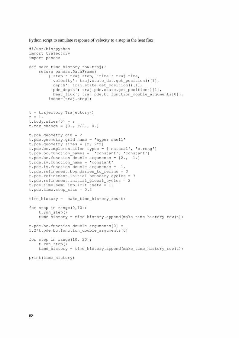
68
Python script to simulate response of velocity to a step in the heat flux
#!/usr/bin/python
import trajectory
import pandas
def make_time_history_row(traj):
return pandas.DataFrame(
{'step': traj.step, 'time': traj.time,
'velocity': traj.state_dot.get_position()[1],
'depth': traj.state.get_position()[1],
'pde_depth': traj.pde.state.get_position()[1],
'heat_flux': traj.pde.bc.function_double_arguments[0]},
index=[traj.step])
t = trajectory.Trajectory()
r = 1.
t.body.sizes[0] = r
t.max_change = [0., r/2., 0.]
t.pde.geometry.dim = 2
t.pde.geometry.grid_name = 'hyper_shell'
t.pde.geometry.sizes = [r, 2*r]
t.pde.bc.implementation_types = ['natural', 'strong']
t.pde.bc.function_names = ['constant', 'constant']
t.pde.bc.function_double_arguments = [2., -1.]
t.pde.iv.function_name = 'constant'
t.pde.iv.function_double_arguments = -1.
t.pde.refinement.boundaries_to_refine = 0
t.pde.refinement.initial_boundary_cycles = 3
t.pde.refinement.initial_global_cycles = 2
t.pde.time.semi_implicit_theta = 1.
t.pde.time.step_size = 0.2
time_history = make_time_history_row(t)
for step in range(0,10):
t.run_step()
time_history = time_history.append(make_time_history_row(t))
t.pde.bc.function_double_arguments[0] =
1.2*t.pde.bc.function_double_arguments[0]
for step in range(10, 20):
t.run_step()
time_history = time_history.append(make_time_history_row(t))
print(time_history)

69
B. Code excerpts
ExtrapolatedField, derived from deal.II’s FEFieldFunction
#include <deal.II/base/function.h>
#include <deal.II/grid/grid_tools.h>
#include <deal.II/numerics/fe_field_function.h>
using namespace dealii;
template<int dim>
class ExtrapolatedField : public Function<dim>
{
public:
ExtrapolatedField(const DoFHandler<dim> &dof_handler,
const Vector<double> &f)
: Function<dim>(),
field(dof_handler, f),
dof_handler_sp(&dof_handler, "ExtrapolatedField")
{}
virtual double value(const Point<dim> &point,
const unsigned int component = 0) const;
private:
Functions::FEFieldFunction<dim> field;
SmartPointer<const DoFHandler<dim>,ExtrapolatedField<dim>> dof_handler_sp;
Point<dim> get_nearest_boundary_vertex(const Point<dim> &point) const;
};
template<int dim>
double ExtrapolatedField<dim>::value(const Point<dim> &point,
const unsigned int component) const
{
Assert(component == 0, ExcInternalError());
double val;
try
{
val = field.value(point, component);
}
catch (GridTools::ExcPointNotFound<dim>)
{
val = field.value(get_nearest_boundary_vertex(point));
}
return val;
}
template <int dim>
Point<dim> ExtrapolatedField<dim>::get_nearest_boundary_vertex
(const Point<dim> &point) const
{
double arbitrarily_large_number = 1.e32;
double nearest_distance = arbitrarily_large_number;
Point<dim> nearest_vertex;
for (auto cell : dof_handler_sp->active_cell_iterators())
{
if (!cell->at_boundary())
{
continue;
}
for (unsigned int f=0; f<GeometryInfo<dim>::faces_per_cell; ++f)
{
if (!cell->face(f)->at_boundary())
{
continue;
}
for (unsigned int v=0; v < GeometryInfo<dim>::vertices_per_face; ++v)
{
Point<dim> vertex = cell->face(f)->vertex(v);
double distance = (point - vertex).norm_square();
if (distance < nearest_distance)
{
nearest_vertex = vertex;
nearest_distance = distance;
}
}
}
}