ryuta ray kato - ipss.go.jp

Japanese Journal of Social Security Policy, Vol.9, No.1 (March 2012)

The Impact of Marginal Tax Reforms on the Supply of Health Related Services in Japan*

Ryuta Ray Kato

1. IntroductionThis paper presents a computable general equilib-rium (CGE) framework to numerically examine the impact of so called marginal tax reforms of health related service sectors in Japan.

This paper uses the latest Input-Output table of Japan of year 2005 with 108 different produc-tion sectors, and it explores the effect of marginal changes in tax and subsidy policies from the cur-rent situation on economic efficiency, particularly by targeting three important sectors in health related services; hospital service, social welfare service, and long-term care for the elderly ser-vice sectors. (1) The main purpose of this paper is to evaluate the effect on the supply side of these three service sectors, so that the tax and subsidy of these sectors are particularly considered. By using the actual input-output table, the paper has successfully realized the real Japanese economy within the model, and it tries to present welfare-enhancing reforms within these three sectors.

A distinctive feature of this paper is to focus on the supply side of these sectors, all of which will play a more important role in aging Japan in the near future. The literature on an aging popula-tion of Japan mainly discusses the effect on public schemes such as the public pension, and public health insurance schemes, since its main concern is with financial burdens of population aging on public schemes. It is forecasted not only that population aging will generate more burdens on future and working generations through the cur-rent schemes, but also that the total number of a population will drastically shrink in the future Japan. A future decrease in the total population would likely result in decreasing future GDP, and stable economic growth of the Japanese economy needs a merging sector to stimulate the economy in an aging Japan. An aging population will induce more demand for services provided by these three sectors, and these sectors will be more important to stimulate the Japanese economy. Both private and public enterprises in these three sectors have already been taxed and subsidized in the current scheme, and the government can thus navigate these sectors with several tax and subsidy policies in order to achieve higher economic growth. This

paper numerically examines the effect of several marginal departures from the current tax and sub-sidy policy within a CGE model, and it explicitly considers the budget constraint of the govern-ment. Any policy change should be followed by a secondary policy in order to fulfill the budget constraint, and this paper tries to present realistic policy scenarios to compensate a sector which will suffer from the policy change.

Simulation results are as follows. First of all, an expansion of the subsidy to the hospital sector cre-ates the largest welfare gain when the government does not take into account its financing explicitly. While such an expansion policy improves eco-nomic efficiency, it also induces a certain amount of government deficits. However, the effect of such a policy on economic efficiency is more than ten times as much as the cost. For instance, the amount of newly generated government deficits is 5.3 billion Japanese yen when the net subsidy rate of the hospital sector increases by 50% from the current level, while the improvement in economic efficiency by the policy is measured to be 72.3 billion Japanese yen. Secondly, however, such an expansion policy does necessarily not eventuate in the largest gain if the government considers its balanced budget. The reduction of the subsidy to the hospital sector results in the largest welfare gain to the whole economy if the government uses the government surplus induced by the reduction of the subsidy in order to decrease the tax imposed on the social welfare sector. When the subsidy to the hospital sector is reduced by 50% from the current level, then the expected welfare gain to the whole economy would be approximately 3.8 billion Japanese yen, if the government surplus created by the 50% reduction of the subsidy to the hospital sector is used to reduce the tax on the social welfare sector. In fact, the 50% reduction of the subsidy to the hospital sector eventuates in the social welfare sector being subsidized. Finally, if the hospital sector is compensated by lump-sum transfers when its subsidy is reduced, then a wel-fare gain could become larger. If the government uses the government surplus not only for reduc-ing the tax on the social welfare sector but also for providing the hospital sector with lump-sum

1

107

i =1

107i =1

107

i =1


transfers in order to keep income of the hospital sector unchanged, then a larger welfare gain would be obtained, even if the government implements a balanced budget policy. When the government reduces the subsidy to the hospital sector by 50% from the current level, the expected welfare gain to the whole economy is 11.15 billion Japanese yen. Such a policy keeps the total income of the hospital sector unchanged by lump-sum transfers, and also increases the total income of the social welfare sector by reducing its tax. This implies that a welfare enhancing tax reform within the health related sectors is plausible as long as the subsidy to the hospital sector can be reduced. Such a reform does not create any new government defi-cit either.

The paper is organized as follows. The next section explains the data and numerical model, and Section 3 simulates several scenarios with results and evaluations. Section 4 concludes the paper.

2. Data and ModelThis paper employs the conventional static com-putable general equilibrium (CGE) model with the actual and the latest input-output table of Japan of year 2005. Note that all parameter values in the model are calculated by using the actual data, so that the calculated values of endogenous variables obtained within the model also become quite real-istic.

2.1 DataThe latest input-output table of Japan of year 2005 with 108 different intermediate sectors has been used in order to construct the social accounting matrix (SAM). The SNA data has also been used to obtain the amount of aggregate private savings. The last sector, namely the 108th sector, includes all unclassified items. Since the value of its factor payments of some intermediate sectors becomes negative (2), this paper has integrated the 108th sec-tor with the 106th sector which includes all other services. The integration makes the actual input-output table data consistent to the model, and it is assumed in this paper that there are 107 differ-ent production sectors, all of which are allowed to have intermediate production processes. Based on this simplification, the social accounting matrix (SAM) has been made. Then this paper particu-larly pays more attention to the following three sectors in health related services; Medical Ser-vice and Health (i = 94), Social Security (i = 95), and Nursing Care (i = 96).(3) The main sector in Medical Service and Health (i = 94) is the hospital sector. Social Security (i = 95) includes economic activities of nurseries, nursing homes, social

welfare centers, and administrative work of the public pension as well as public health insurance schemes. Nursing Care (i = 96) shows economic activities of the industry of the long-term care for the elderly.

Figure 1 shows economic values of domestic final consumption goods of these three sectors in the latest input-output table of year 2005. Medical Service and Health (i = 94) is much larger than other sectors, and its value is 37 thousands billion Japanese yen, while the economic values of other two sectors are between 6.4 thousands billion and 6.6 thousands billion Japanese yen, which are less than 18% of the value of Medical Service and Health (i = 94) sector.

2.2 ModelThe computable general equilibrium model of this paper employs the conventional static model.(4) The Japanese economy is assumed to consist of 107 different sectors, households, the government, and the investment firm sector. All 107 industries are allowed to have intermediate production pro-cesses, and they are assumed to maximize their profit. Households are assumed to maximize their utility over 107 different consumption goods. The government is assumed to determine its tax rev-enue, the amount of subsidies, and its consump-tion in order to satisfy its budget constraint. The economy is assumed to be fully competitive, so that all prices are determined in the relevant mar-kets in order to equate the amount of demand to the amount of supply at its fully competitive price level in equilibrium. Note that the model is static and thus the short-run effect is only investigated. Thus, it is assumed for simplicity that factor inputs are not mobile among different sectors in the short-run.

<Households>Households are assumed to be homogenous, and their utility is given by:

U (X1 , X2 , …, X107) = Π Xiαi, (1)

where X1 denotes consumption of good i. ∑ αi = 1 is assumed. i denotes each sector. The parameter value of each αi is determined by using the actual social accounting matrix, which is given in Table 6.

Households are assumed to maximize (1) with respect to their consumption goods subject to their budget constraint such that:

∑ pi Xi = I (1 – τI) – SI,

2

107

i =1

107

i =1

αi I (1– τI ) (1– sI )pi

pi Xi

I (1– τI ) (1– sI )pi Xi

(1– sI ) (1– τI ) (∑ rj Kj + ∑ wj Lj)107j =1

107j =1


where pi and I denote the price of good i and income, respectively. τI is the proportional income tax rate, and it is calculated by using the actual social accounting matrix. SI denotes the amount of savings, and households are assumed to save the constant amount relative to their disposal income. The amount of savings is assumed to be given by

SI = sI (1– τI ) I,

where the constant ratio, sI, is given exog-enously.(5) The value of sI has been calculated by using the actual SAM. Then income is given by

I = ∑ ri Ki + ∑ wi Li

where r and w denote the rental cost and the wage rate, respectively. K and L are endowments of capital and labour, respectively. The factor pay-ments change as r or w changes. Note that the amounts of ri Ki and wi Li are both obtained from the actual social accounting matrix.

The first order conditions yield the demand functions such that:

Xi = Xi ( pi, Y; αi ) = , i

= 1, 2, …, 107. (2)

Note that αi can be calculated by using (2) and the actual social accounting matrix so that:

αi =

= , i

= 1, 2, …, 107,

where both the values of the denominator and the numerator can be obtained from the actual social accounting matrix. The estimated values of αi are given in Table 6.

<Private Firms>Following the conventional assumption, the mul-tiple decisions by each firm are described by the tree structure, where each firm is assumed to make a decision over several different items. In the tree structure, the optimal behavior of each firm which makes a decision over different items is described as if the firm always makes a decision over two different items at different steps. Each firm makes a decision over different items; the amount of exports of its own product, the amount of imported goods and intermediate goods used for its produc-tion, and the amount of labor and capital. This

assumption simplifies a complicated decision over several items by each rm. Each step is also shown in Figure 2.

At step 1, a private firm, i , is assumed to use labor and capital to produce its composite goods, Yi . Then, the firm is assumed to produce its domestic goods, Z i , by using its own Yi and Z i, j at the second step. X i, j denotes the final consump-tion goods produced by firm j used by firm i for its production. Thus, X i, j is the amount of the final consumption goods produced by firm j for the intermediate production process of firm i. At the third step, the firm is assumed to decompose its domestic goods, Z i , into exported goods, Ei , and final domestic goods, Di . This step is concerned about its optimal decision over the amount of its product to be exported. At the final step (the fourth step), the firm is assumed to produce its final con-sumption goods, Qi , by using its final domestic goods, Di , and imported goods, Mi . This step cor-responds to its optimal decision over how much it uses imported goods, Mi , and its own goods, Di , to produce its final consumption goods, Qi , which are consumed by domestic households. The assump-tion of this tree structure in terms of different deci-sions can incorporate firm’s complicated decisions over the amount of exports of its own product, the amount of imported goods and intermediate goods which the firm uses in its production process, and the amount of factor inputs into the model in a tractable way.

Note that all market clearing conditions are used to determine all prices endogenously in their corresponding markets, and also that at each step the private firm is assumed to determine the amount of relevant variables in order to maximize its profit.

By the assumption of the above tree structure, all decision making processes can be simplified, and the optimal behavior about all different deci-sions can be incorporated as follows:

Step 1: The production of composite goods Each firm is assumed to produce its composite goods by using capital and labor. Each firm is assumed to maximize its profit given by:

πi = piY Yi (K i , L i ) – ri Ki – wi L i , (3)

where Yi and piY denote the composite goods

produced by firm i and its price, respectively. K i and L i denote capital and labor used by firm i in order to produce its composite goods, respectively. The production technology is given by:

Yi (K i , L i ) = K iβK, i L i

βL, i, i = 1, 2, …, 107, (4)

3

βK, i

ri

βL , i

wi

ri Ki

piY Yi

wi Li

piY Yi

Yi Xi, j

107

j

Xi, j

axi, j

Yi

ayi

107

j

ei

dii

κie (1+ τ i

p – τ is ) pi

Z Zi

pie

κid (1+ τ i

p – τ is ) pi

Z Zi

pid

pie Ei

(1+ τ ip – τ i

s ) piZ Zi

pid Di

(1+ τ ip – τ i

s ) piZ Zi


where βK, i + βL, i is assumed for all i = 1, 2, …, 107. Each firm is assumed to maximize (3) with respect to labor and capital subject to (4), and the first order conditions yield the demand functions such that:

K i = K i ( piY, ri , wi ; βK, i , βL, i ) = pi

Y Yi , (5a)

L i = L i ( piY, ri , wi ; βK, i , βL, i ) = pi

Y Yi , i

= 1, 2, …, 107. (5b)

Note that βK, i and βL, i can be calculated by using (5a), (5b), and the actual social accounting matrix so that:

βK, i = ,

βL, i = , i = 1, 2, …, 107,

where ri Ki , and wi Li can be obtained from the actual social accounting matrix.

The estimated values of βK, i and βL, i are given in Table 6.

Step 2: The production of domestic goods Each firm is assumed to produce domestic goods, Zi, by using intermediate goods and its own com-posite goods, which production has been described at step 1. The optimal behavior of each firm in terms of the production of domestic goods can be described such that:

Maxπi = piZ Zi – pi

Y Yi – ∑ pjX Xi, j ,

st Zi = min , , i = 1, 2, …, 107,

where Xi, j and pjX denote intermediate good

used by firm j and i its price, respectively. piZ is the

price of Zi . axi, j denotes the amount of intermedi-ate good j used for producing one unit of a domes-tic good of firm i, and ayi denotes the amount of its own composite good for producing one unit of its domestic good. The estimated values of ayi are given in Table 6.(6) Note that the production func-tion at this step is assumed to be the Leontief type. Using axi, j and ayi , and assuming that the market is fully competitive, the zero-profit condition can be written by:

piZ = pi

Y ayi + ∑ pjX axi, j , i = 1, 2, …, 107.

Step 3: Decomposition of Domestic Goods into Exported Goods and Final Domestic GoodsThe optimal decision made by firm i in terms of the amount of exports of its own goods is described as the decomposition of Zi (i = 1, 2, …, 107) into exported goods, Ei, and final domestic goods, Di . Each firm is assumed to maximize its profit such that:

πi = pie Ei + pi

d Di – (1+ τ ip – τ i

s ) piZ Zi , (6)

where pie and pi

d denote the price when the domestic goods are sold abroad, and the price when the domestic goods are sold domestically, respectively. Note that pi

e is measured in the domestic currency. τ i

p and τ is are the tax rates of

a production tax imposed on the production of Zi and the subsidy rate, respectively. The values of τ i

p and τ is are calculated by using the actual social

accounting matrix, and the calculated values are given in Table 2-1 and 2-2. The decomposition is assumed to follow the Cobb-Douglas technology such that:

Zi = Eiκ Di

κ , i = 1, 2, …, 107, (7)

where κid + κ i

e = 1 (i = 1, 2, …, 107) is assumed. Each firm is assumed to maximize (6) with respect to Ei and Di subject to (7), and the first order conditions yield

Ei = Ei ( pie, pi

d, piZ; τ i

p, τ is, κi

d, κie) =

, (8a)

Di = Di ( pie, pi

d, piZ; τ i

p, τ is, κi

d, κie) =

, i = 1, 2, …, 107, (8b)

Note that κie and κi

d can be calculated by using (8a), (8b), and the actual social accounting matrix so that:

κie = ,

κid = , i = 1, 2, …, 107,

where pie Ei , pi

d Di , τ is pi

Z Zi , and τ ip pi

Z Zi can be obtained from the actual social accounting matrix. The estimated values of κi

e and κid are given in

Table 6.

4

mi

di

γ im piQ Qi

(1+ τ im ) pi

m

γ id piQ Qi

pid

(1+ τ im ) pi

m Mi

piQ Qi

pid Di

piQ Qi

107

i =1

107

i =1

107

i =1

107

i =1

107

i =1

107

i =1

107

i =1

107

i =1


Step 4: The Production of the final goodsDenote the final consumption goods by Qi (i = 1, 2, …, 107). The final consumption goods are assumed to be produced by using the final domes-tic goods, Di , and the imported goods, Mi . This step corresponds to the optimal decision making behavior of each firm in terms of the amount of imported goods which are used in its production process. The production technology at this final step is given by the following Cobb-Douglas func-tion:

Qi = Miγ Di

γ , i = 1, 2, …, 107, (9)

where γ im + γ id = 1 (i = 1, 2, …, 107) is assumed. Each firm is assumed to maximize its profit with respect to Mi and Di subject to (9). Its profit is given by:

πi = piQ Qi – (1+τ i

m ) pim Mi – pi

d Di , i = 1, 2, …, 107,

where piQ and τ i

m denote the price of its final consumption goods, Qi , and the import tariff rate, respectively. The import tariff rate is calculated by using the actual social accounting matrix, and it is given in Table 2-4. Then, the first order conditions yield

Mi = Mi ( pim, pi

d, piQ; τ i

m, γ im, γ i

d )

= , (10 a)

Di = Di ( pim, pi

d, piQ; τ i

m, γ im, γ i

d )

= , i = 1, 2, …, 107, (10 b)

Note that γ im and γ id can be calculated by using (10a), (10b), and the actual social account-ing matrix so that:

γ im = ,

γ id = , i = 1, 2, …, 107,

where pimMi , pi

d Di, piQ Qi and τ i

m pimMi

can be obtained from the actual social accounting matrix. The estimated values of γ im and γ id are given in Table 6.

<The Government>The government is assumed to impose several taxes to satisfy its budget constraint. Its budget constraint is given by:

∑ piQ X i

g + Sg + Sub = T I + T p + T m,

where the left hand side is the total govern-ment expenditure, and the right hand side is the total government revenue. X i

g and Sg denote gov-ernment consumption of final consumption good i; and government savings, respectively. Sub denotes the total amount of subsidies such that:

Sub = ∑ τ is ( p iz Zi ).

The total tax revenue is given by:

T I = τ I I = τ I ∑ ri Ki + ∑ wi L i ,

T p = ∑ τ ip ( p iz Zi ),

T m = ∑ τ im ( p im Mi ),

where T I, T p and T m denote the total income tax revenue, the total production tax revenue, and the total import tariff revenue, respectively. The government is assumed to save the constant amount relative to the total amount of tax revenue, and the government savings are assumed to be given by

Sg = sg ( T I + T p + T m),

where the constant ratio, Sg, is given exoge-nously, and .its value has been calculated by using the actual SAM.

<Equilibrium Conditions>There are two factor inputs, labour and capital. Since the model is static and thus the short-run effect is explored, it is assumed that each factor cannot move among different sectors (industries) in the short-run. This implies the equilibrium con-ditions of factor markets such that

Ki = Ki, (11 a)

Li = Li , i = 1, 2, …, 107, (11 b)

where the total amount of endowments is given by:

K = ∑ Ki ,

L = ∑ Li ,

Note that ri and wi (i = 1, 2, …, 107) are determined in order to satisfy (11a) and (11b), respectively.

In terms of the market clearing condition of good i (i = 1, 2, …, 107); a private investment sector is introduced in order to close the economy in this

5

107

j

107

i =1

107

i =1

107

i =1


paper.(7) Denoting the amount of good i consumed by the private investment sector by Xi

s, the market clearing condition of good i is given by:

Qi = Xi + Xig + Xi

s + ∑ Xij ,i = 1, 2, …, 107, (12)

where the left hand side is the total supply, and the right hand side is the total demand for good i. pi

Q (i = 1, 2, …, 107) is determined in order to satisfy (12). Note that the budget constraint of the private investment sector is given by:

∑ piQ Xi

s = S g + S I + S f,

where the left hand side is the total amount of its consumption, and the right hand side is the total amount of its income. S f denotes the total amount of savings by the foreign sector, or the deficits in the current account, and it is given by subtracting exports from imports.(8) Since both the amount of exports and the amount of imports can be obtained from the actual social accounting matrix, S f can be calculated from the actual social accounting matrix, and thus it is exogenously given in the model. Furthermore, the foreign trade balance is given by

∑ piw, e Ei + S f = ∑ pi

w, m Mi ,

where piw, e and pi

w, m denote the world price of export goods, and import goods of good i, respec-tively, and both of them are assumed to be given exogenously. Since pi

e and pim are both measured

in the domestic currency, they are also expressed such that:

pie = ε pi

w, e,

pim = ε pi

w, m, i = 1, 2, …, 107,

where ε denotes the exchange rate. Note that the exogeneity assumption on the world prices implies that the exchange rate is endogenously determined within the model.

3. Simulation Analysis3.1 Benchmark and CalibrationThe benchmark case should reflect the real Japa-nese economy in order to make the subsequent simulation scenarios realistic. Thus, the bench-mark model should carefully be calibrated until the calculated values of all endogenous variables within the model become close to the actual values. Table 1-1 to 1-4 show the calculated model values as well as the corresponding actual values in year 2005. As shown in these tables, the benchmark case

has successfully been able to reproduce the real economy within the model. Note that the tax rates and the subsidy rates shown in Table 2-1 to 2-4 have been calculated by using the actual amount of tax and subsidy, so that they can be interpreted as the average proportional rates.

Table 2-3 particularly shows the net rate, which is defined as the difference between the pro-duction tax rate and the subsidy rate. The negative value of the net rate implies that the sector is sub-sidized by a certain amount.(9) As Table 2-3 shows, only Medical Service and Health (i = 94: hospital sector) is subsidized (net subsidy rate: 0.3432%) among all relevant three sectors. Since the effect of changes in the net rate is only simulated in the subsequent sections, the net rates of these three sectors are shown again in Table 2-3-1. Note also that welfare gains in the next section are all measured by equivalent variation (EV), so that the effect of policy changes on economic efficiency are measured financially.

3.2 Simulations3.2.1 Scenario I without balanced budgetAny policy change should be followed by a sec-ondary policy if the budget constraint of the gov-ernment is fulfilled even after the policy change. In this paper, the total government expenditure is assumed to be unchanged even after a policy change. This implies that the total revenue should be unchanged in order to fulfill the budget con-straint, so that any policy change should be fol-lowed by a secondary policy in order to satisfy the budget constraint.

However, a secondary policy conducted in order to fulfill the budget constraint obviously generates another effect on an economy, so that it is very difficult to separate the obtained result into the effects of the first and second policies, respec-tively. Then, Table 3-1 shows the pure effect of a policy change without a secondary policy based on the assumption that the gap between revenue and expenditure caused by any policy change is financed by government bonds implicitly. While the budget is not balanced after a policy change, it can show how much the Japanese government needs to conduct marginal tax/subsidy reforms. Note that Table 3-1 shows to the extent how much economic gains would be obtained by changing the net rate of each sector from the current level under the assumption that the temporary budget is not balanced. The negative value of government deficits in the table implies that government sur-plus will be generated by a policy change. Since the economic size of Medical Service and Health (i = 94: hospital sector) is much larger than other

6


two sectors, an increase in the subsidy to Medical Service and Health (i = 94: hospital sector) results in the largest welfare gain. For instance, if the gov-ernment increases the net subsidy rate of this sector by 50% from the current level, then the expected gain in economic efficiency is measured to be 72.3 billion Japanese yen with newly generated government deficits of approximately 5.6 billion Japanese yen. However, note that the overall effect of such a policy is more than ten times as much as the cost, since the amount of newly generated government deficits (5.3 billion Japanese yen) is less than one tenth of a welfare gain (72.3billion Japanese yen).

3.2.2 Scenario II with balanced budgetIn this scenario, the budget constraint is explic-itly fulfilled with a secondary tax/subsidy policy. While it is possible to consider many second-ary policies to fulfill the budget constraint, it is assumed that the net rates of three sectors are only considered. Note that both the production tax and the subsidy are distortionary. Since the net rate is modified from the current level, the environment considered in this paper is the second-best situa-tion, implying that the overall effect on economic efficiency might be positive or negative as pointed out by Lipsey and Lancaster (1956). The sector, which net rate is modified exogenously, is called the initial sector, and the sector, which net rate is adjusted endogenously in order to fulfill the budget constraint, is called the secondary sector. Table 3-2 shows the overall effect of such poli-cies. A striking result is that when the budget is balanced by a secondary policy the result is quite different. If the balanced budget is not considered explicitly, the most effective welfare enhancing policy is to more subsidize Medical Service and Health (i = 94: hospital sector).However, if the gap between revenue and expenditure caused by the initial policy change is financed by a distortionary tax/subsidy policy within the health related sec-tors, then the reduction of the subsidy to Medical Service and Health (i = 94: hospital sector) is more preferable oppositely. While a policy to expand the subsidy to Medical Service and Health (i = 94: hospital sector) still eventuates in a welfare gain irrespective of a secondary policy, a welfare gain generated by a policy to reduce the subsidy fol-lowed by a secondary policy to adjust the net rate of Social Security (i = 95) is the largest. When the net subsidy rate of Medical Service and Health (i = 94: hospital sector) is reduced by 50% from the current level, the expected welfare gain is 3.78 bil-lion Japanese yen if the policy is followed by the endogenous adjustment of the net rate of Social

Security (i = 95) sector.As long as the effect on economic efficiency

of the whole economy with the balanced budget is concerned, a reform with the reduction of the sub-sidy to Medical Service and Health (i = 94: hospital sector) sector followed by an endogenous tax cut in Social Security (i = 95) sector is most effective. However, such a policy results in a decrease (an increase) in the total income of Medical Service and Health (i = 94: hospital sector) sector. Table 4-1 shows that while the total income of Social Security (i = 95) sector is expected to increase by 1.0188% from the current level, that of Medical Service and Health (i = 94: hospital sector) sec-tor is expected to decrease by 0.1756%. Table 4-2 also shows that such a policy eventuates 17 in Social Security (i = 95) sector being subsidized. This is because the economic size of Medical Service and Health (i = 94: hospital sector) sec-tor is much larger than that of Social Security (i = 95) sector, so that a 50% reduction of the subsidy rate of Medical Service and Health (i = 94: hos-pital sector) sector induces a huge amount of the government surplus, resulting in the government subsidizing Social Security (i = 95) sector. Such a policy is obviously favorable for Social Security (i = 95) sector, but it is not for Medical Service and Health (i = 94: hospital sector) sector. Since the economic size of Medical Service and Health (i = 94: hospital sector) is quite large, it seems politically difficult to implement such a policy. Then in the next scenario, a compensation policy is investigated.

3.2.3 Scenario III with balanced budget and a compensation policy

Scenario II shows that the reduction of the subsidy to Medical Service and Health (i = 94: hospital sector) sector followed by a decreasing tax policy of Social Security (i = 95) sector results in the largest welfare gain to the whole economy. Thus, Scenario III only investigates the case where the net tax rate of Social Security (i = 95) sector is endogenously modified as a secondary policy in order to full the budget constraint. Furthermore, Scenario III assumes that Medical Service and Health (i = 94: hospital sector) sector is com-pensated by lump-sum transfers, so that the total income of Medical Service and Health (i = 94: hospital sector) sector keeps unchanged even after an exogenous decrease in its net subsidy rate. Table 5 shows the striking result. When the net subsidy rate of Medical Service and Health (i = 94: hospital sector) sector is reduced by 50% from the current level, a welfare gain to the whole economy is measured to be 11.15 billion Japanese

7


yen, which is much larger than the case where all government surplus generated by the reduction of the subsidy is used to decrease the tax on Social Security (i = 95) sector. If the surplus is only used for the reduction of the tax on Social Security (i = 95) sector, then expected amount of a welfare gain is only 3.78 billion Japanese yen as shown in Table 3-2. While the net tax rate for Social Security (i = 95) sector is higher in Scenario III compared to Scenario II, it still obtains an increase in its income, since its net rate can be reduced by such a policy. This implies that it is plausible to enhance welfare (economic efficiency) even in the health related sectors if the amount of the subsidy to Medical Service and Health (i = 94: hospital sector) sector can be reduced. Note that Scenario III uses non-distortionary lump-sum transfers in order to compensate Medical Service and Health (i = 94: hospital sector) sector. In Scenario III, the distortionary subsidy to Medical Service and Health (i = 94: hospital sector) sector and the dis-tortionary tax on Social Security (i = 95) sector are both reduced, and the government surplus is redistributed to Medical Service and Health (i = 94: hospital sector) sector by lump-sum transfers. Note also that the amount of lump-sum transfers is more than three times as much as a welfare gain to the whole economy. This implies that the govern-ment has to redistribute lots of resources through transfers to improve economic efficiency if the government tries to reform health related produc-tion sectors.

4. Concluding RemarksThis paper has presented a computable general equilibrium (CGE) framework to numerically examine the effect of marginal tax reforms on the supply side of health related sectors in Japan. This paper has used the latest Input-Output table of Japan of year 2005 with different production sectors.

Several simulations have been conducted in comparison with a very realistic benchmark model, and the obtained results are as follows. First of all, an expansion of the subsidy to the hospital sector creates the largest welfare gain when the government does not take into account its financ-ing explicitly. While such an expansion policy improves economic efficiency, it also induces a certain amount of government deficits. However, the effect of such a policy on economic efficiency is more than ten times as much as the cost. For instance, the amount of newly generated govern-ment deficits is 5.3 billion Japanese yen when the subsidy to the hospital sector increases by 50%

from the current level, while the improvement in economic efficiency by the policy is measured to be 72.3 billion Japanese yen. Secondly, however, such an expansion policy does necessarily not eventu-ate in the largest gain if the government considers its balanced budget. The reduction of the subsidy to the hospital sector results in the largest welfare gain to the whole economy if the government uses the government surplus induced by the reduction of the subsidy in order to decrease the tax imposed on the social welfare sector. When the subsidy to the hospital sector is reduced by 50% from the current level, then the expected welfare gain to the whole economy would be approximately 3.8 billion Japanese yen, if the government surplus created by the 50% reduction of the subsidy to the hospital sector is used to reduce the tax on the social welfare sector. In fact, the 50% reduction of the subsidy to the hospital sector eventuates in the social welfare sector being subsidized. Finally, if the hospital sector is compensated by lump-sum transfers when its subsidy is reduced, then a wel-fare gain could become larger. If the government uses the government surplus not only for reducing the net tax rate of the social welfare sector but also for providing the hospital sector with lump-sum transfers in order to keep income of the hospital sector unchanged, then a larger welfare gain would be obtained, even if the government implements a balanced budget policy. When the government reduces the subsidy to the hospital sector by 50% from the current level, the expected welfare gain to the whole economy is 11.15 billion Japanese yen. Such a policy keeps the total income of the hospital sector unchanged by lump-sum transfers, and also increases the total income of the social welfare sector by reducing its tax. This implies that a welfare enhancing tax reform within the health related sectors is plausible as long as the subsidy to the hospital sector can be reduced. Such a reform does not create any new government defi-cit either.

While this paper has used the Japanese input-output table, it is applicable to all other countries in order to investigate the effect of several health policies. By explicitly considering the budget con-straint within a computable general equilibrium framework, this paper has thrown light on the importance of explicit consideration of the gov-ernment budget constraint when simulations on tax and subsidy policies are conducted.

Ryuta Ray Kato, Ph.D (Graduate School of Inter- national Relations)

8


Notes*) Keywords: Computable General Equilibrium

(CGE) Model, Marginal Tax Reform, Health Sectors, Taxation, Subsidy, Simulation; JEL Classification: C68, H51, and H53.

1) Kato (2011) also discusses the effect of reforms on the supply side of the pharma-ceutical industry.

2) Labor income and capital income are factor payments.

3) The numbers in the brackets are numbers allocated to the sectors in the actual input-output table of year 2005 with 108 different production sectors.

4) In terms of the conventional static model, see Ballard, Fullerton, Shoven, and Whalley (1985), Shoven and Whalley (1992), and Scarf and Shoven (2008). In particular, the model used in this paper is similar to Hosoe, Ogawa, and Hashimoto (2004). Regarding the dynamic model, it is conventional to employ an overlapping generations model In terms of computable overlapping generations model within a general equilibrium frame-work, see Auerbach and Kotlikoff (1987). Kato (1998), Kato (2002b), Kato (2002a), Ihori, Kato, Kawade, and Bessho (2006), and Ihori, Kato, Kawade, and Bessho (2011) also apply the dyanamic model to several policies in Japan.

5) The assumption that the ratio is exogenously given is made only for the model to be consistent to the actual social accounting matrix, and this assumption is very common in the literature.

6) The estimated values of axij are not presented in Table 2, since the number of the estimated values reach 11,449. The estimated values are given upon request.

7) This is also the conventional assumption in the literature.

8) The FDI is assumed to be negligible in this paper.

9) A tariff is differently treated, so that the net rate is defined above.

ReferencesAuerbach, A. J., and L. J. Kotlikoff (1987):

Dynamic Fiscal Policy. Cambridge Univer-sity Press.

Ballard, C. L., D. Fullerton, J. B. Shoven, and J. Whalley (1985): A General Equilibrium Model for Tax Policy Evaluation. Chicago University Press.

Hosoe, N., K. Ogawa, and H. Hashimoto (2004): Textbook of Computable General Equilib-rium Modeling. University of Tokyo Press.

Ihori, T., R. R. Kato, M. Kawade, and S. Bessho (2006): “Public Debt and Economic Growth in an Aging Japan,” in Tackling Japan’s Fiscal Challenges, ed. by K. Kaizuka, and A. O. Krueger. Palgrave.

— (2011): “Health Insurance Reform and Economic Growth: Simulation Analysis in Japan,” Japan and the World Economy, Forthcoming.

Kato, R. R. (1998): “Transition to an aging Japan: Public pension, savings, and capital taxation,” Journal of the Japanese and Inter-national Economies, 12, 204-231.

— (2002a): “Government deficit, public invest-ment, and public capital in the transition to an aging Japan,” Journal of the Japanese and International Economies, 16, 462-491.

— (2002b): “Government deficits in an aging Japan,” in Government Deficit and Fiscal Reform in Japan, ed. by T. Ihori, and M. Sato. Kluwer Academic Publishers.

— (2011): “Who Has to Pay More, Health Ser-vice Sectors, the Pharmaceutical Industry, or Future Generations?: A Computable General Equilibrium Approach,” Economics and Management Series, IUJ Research Institute, EMS-2011-11.

Lipsey, R. G., and K. Lancaster (1956): “The General Theory of Second Best,” The Review of Economic Studies, 24(1), 11-32.

Scarf, H. E., and J. B. Shoven (eds.) (2008): Applied General Equilibrium Analysis. Cambridge University Press.

Shoven, J. B., and J. Whalley (1992): Applying General Equilibrium. Cambridge University Press.

9

40,000

35,000

30,000

25,000

20,000

15,000

10,000

5,000

0

i = 94: Medical Service and Health Sector (incl. hospitals)i = 95: Social Security Sector (incl. nurseries, nursing homes, social welfare centers, and administrative work of public schemes)i = 96: Nursing Care Sector (incl. long term care for the elderly)

Figure 1: Economic Values of the Domestic Final Consumption Goods in the IO Table of Year 2005

Unit: One billion Japanese yen

i = 94 i = 95 i = 96

37,209

6,616 6,388


10

Table 1-1: Economic Values of the Benchmark ModelFinal Consumption Goods, Pi

Q Qi ; i = 1, 2, …, 107Unit: One million Japanese yen

i 1 2 3 4 5 6 7 8 9model 7992445 3076453 867591 1507966 1889503 1673551 997155 13666806 28226829actual 7992445 3076453 867591 1507966 1889503 1673551 997155 13666806 28226829

i 10 11 12 13 14 15 16 17 18model 8448175 1528645 3087907 2024194 5403523 3545906 2864489 4718832 3383067actual 8448175 1528645 3087907 2024194 5403523 3545906 2864489 4718832 3383067

i 19 20 21 22 23 24 25 26 27model 6295844 388535 2014268 2646909 5170128 2438742 417929 7287054 6308055actual 6295844 388535 2014268 2646909 5170128 2438742 417929 7287054 6308055

i 28 29 30 31 32 33 34 35 36model 17484729 1289256 10137398 2776993 1249173 1559315 2988851 716762 1675103actual 17484729 1289256 10137398 2776993 1249173 1559315 2988851 716762 1675103

i 37 38 39 40 41 42 43 44 45model 7818878 11656182 1901806 2113988 3624169 5085451 4791626 7716325 7736765actual 7818878 11656182 1901806 2113988 3624169 5085451 4791626 7716325 7736765

i 46 47 48 49 50 51 52 53 54model 9649963 3346489 3968133 5585456 1924973 2445823 2919353 6776294 4409610actual 9649963 3346489 3968133 5585456 1924973 2445823 2919353 6776294 4409610

i 55 56 57 58 59 60 61 62 63model 4075496 9563708 7856948 2718049 25319384 1004116 3563331 3809563 5232559actual 4075496 9563708 7856948 2718049 25319384 1004116 3563331 3809563 5232559

i 64 65 66 67 68 69 70 71 72model 648298 30715358 9119713 16205999 7196254 15754107 2893277 4549749 3745112actual 648298 30715358 9119713 16205999 7196254 15754107 2893277 4549749 3745112

i 73 74 75 76 77 78 79 80 81model 98358600 41431380 8595547 11913778 45678819 6638078 16293277 9960768 3554235actual 98358600 41431380 8595547 11913778 45678819 6638078 16293277 9960768 3554235

i 82 83 84 85 86 87 88 89 90model 3512957 489752 1786627 6506596 16367961 3678393 17614538 1214895 7440836actual 3512957 489752 1786627 6506596 16367961 3678393 17614538 1214895 7440836

i 91 92 93 94 95 96 97 98 99model 38537877 23178561 13371738 37209390 6616330 6387536 5044458 9175582 11969164actual 38537877 23178561 13371738 37209390 6616330 6387536 5044458 9175582 11969164

i 100 101 102 103 104 105 106 107model 12657970 30319697 10129655 21613601 7671606 6337175 12761623 1517809actual 12657970 30319697 10129655 21613601 7671606 6337175 12761623 1517809



11

Table 1-2: Economic Values of the Benchmark Model (Continued)Capital Income, rK i ; i = 1, 2, …, 107

Unit: One million Japanese yen

i 1 2 3 4 5 6 7 8 9model 3013193 619764 196982 729575 522992 4630 105212 21743 2970822actual 3013193 619764 196982 729575 522992 4630 105212 21743 2970822

i 10 11 12 13 14 15 16 17 18model 1565909 238849 402011 93908 122904 354057 147044 692022 323586actual 1565909 238849 402011 93908 122904 354057 147044 692022 323586

i 19 20 21 22 23 24 25 26 27model 1100374 43932 348142 171629 401898 261535 43896 1438660 727686actual 1100374 43932 348142 171629 401898 261535 43896 1438660 727686

i 28 29 30 31 32 33 34 35 36model 221319 152394 640925 367357 59695 349608 426126 91958 273911actual 221319 152394 640925 367357 59695 349608 426126 91958 273911

i 37 38 39 40 41 42 43 44 45model 778178 1758911 294256 97254 143678 377406 368039 709631 930517actual 778178 1758911 294256 97254 143678 377406 368039 709631 930517

i 46 47 48 49 50 51 52 53 54model 1384756 375474 322166 352810 170457 506256 306073 427506 301195actual 1384756 375474 322166 352810 170457 506256 306073 427506 301195

i 55 56 57 58 59 60 61 62 63model 428739 526290 601345 172999 1211068 207040 332438 377004 433360actual 428739 526290 601345 172999 1211068 207040 332438 377004 433360

i 64 65 66 67 68 69 70 71 72model 42930 1674911 443521 1341333 571988 4231709 403822 1540735 503561actual 42930 1674911 443521 1341333 571988 4231709 403822 1540735 503561

i 73 74 75 76 77 78 79 80 81model 2.50E+07 1.30E+07 3894961 8303863 3.80E+07 2135328 1216237 0 605096actual 2.50E+07 1.30E+07 3894961 8303863 3.80E+07 2135328 1216237 0 605096

i 82 83 84 85 86 87 88 89 90model 246642 54476 316483 2092779 5289614 835932 3579498 229693 967790actual 246642 54476 316483 2092779 5289614 835932 3579498 229693 967790

i 91 92 93 94 95 96 97 98 99model 1.20E+07 3190946 1238479 4579116 283558 807134 366078 1127663 6291773actual 1.20E+07 3190946 1238479 4579116 283558 807134 366078 1127663 6291773

i 100 101 102 103 104 105 106 107model 763930 5863257 3249479 2501464 1084820 1975728 1549710 0actual 763930 5863257 3249479 2501464 1084820 1975728 1549710 0



12

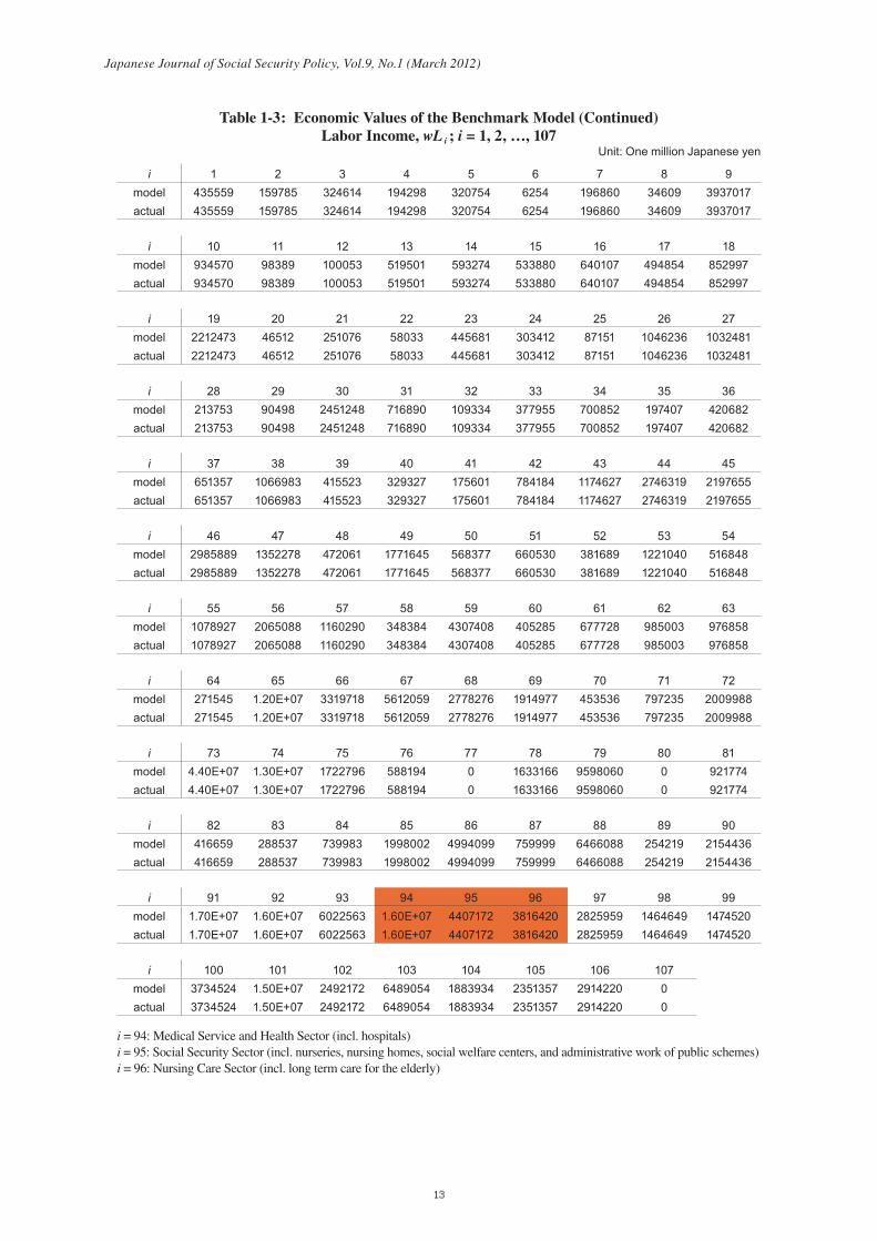
Table 1-3: Economic Values of the Benchmark Model (Continued) Labor Income, wL i ; i = 1, 2, …, 107


i 1 2 3 4 5 6 7 8 9model 435559 159785 324614 194298 320754 6254 196860 34609 3937017actual 435559 159785 324614 194298 320754 6254 196860 34609 3937017

i 10 11 12 13 14 15 16 17 18model 934570 98389 100053 519501 593274 533880 640107 494854 852997actual 934570 98389 100053 519501 593274 533880 640107 494854 852997

i 19 20 21 22 23 24 25 26 27model 2212473 46512 251076 58033 445681 303412 87151 1046236 1032481actual 2212473 46512 251076 58033 445681 303412 87151 1046236 1032481

i 28 29 30 31 32 33 34 35 36model 213753 90498 2451248 716890 109334 377955 700852 197407 420682actual 213753 90498 2451248 716890 109334 377955 700852 197407 420682

i 37 38 39 40 41 42 43 44 45model 651357 1066983 415523 329327 175601 784184 1174627 2746319 2197655actual 651357 1066983 415523 329327 175601 784184 1174627 2746319 2197655

i 46 47 48 49 50 51 52 53 54model 2985889 1352278 472061 1771645 568377 660530 381689 1221040 516848actual 2985889 1352278 472061 1771645 568377 660530 381689 1221040 516848

i 55 56 57 58 59 60 61 62 63model 1078927 2065088 1160290 348384 4307408 405285 677728 985003 976858actual 1078927 2065088 1160290 348384 4307408 405285 677728 985003 976858

i 64 65 66 67 68 69 70 71 72model 271545 1.20E+07 3319718 5612059 2778276 1914977 453536 797235 2009988actual 271545 1.20E+07 3319718 5612059 2778276 1914977 453536 797235 2009988

i 73 74 75 76 77 78 79 80 81model 4.40E+07 1.30E+07 1722796 588194 0 1633166 9598060 0 921774actual 4.40E+07 1.30E+07 1722796 588194 0 1633166 9598060 0 921774

i 82 83 84 85 86 87 88 89 90model 416659 288537 739983 1998002 4994099 759999 6466088 254219 2154436actual 416659 288537 739983 1998002 4994099 759999 6466088 254219 2154436

i 91 92 93 94 95 96 97 98 99model 1.70E+07 1.60E+07 6022563 1.60E+07 4407172 3816420 2825959 1464649 1474520actual 1.70E+07 1.60E+07 6022563 1.60E+07 4407172 3816420 2825959 1464649 1474520

i 100 101 102 103 104 105 106 107model 3734524 1.50E+07 2492172 6489054 1883934 2351357 2914220 0actual 3734524 1.50E+07 2492172 6489054 1883934 2351357 2914220 0



13

Table 1-4: Economic Values of the Benchmark Model (Continued)

Unit: One million Japanese yensavings

private sector government sector foreign sectormodel actual model actual model actual

27265700 27265700 70847256 70847256 -6059608 -6059608

tax and subsidyincome tax production tax import tax subsidy

model actual model actual model actual model actual146907949 146907949 34024445 34024445 4774091 4774091 3506668 3506668

The above figures indicate the total amount.

Table 2-1: Calculated Production Tax RatesTAUP (i) = τ ip; i = 1, 2, …, 107 (Subsidy Rate)

TAUP ( 1) TAUP ( 2) TAUP ( 3) TAUP ( 4) TAUP ( 5) TAUP ( 6) TAUP ( 7) TAUP ( 8) TAUP ( 9)5.9867% 2.5114% 6.1820% 1.2527% 4.3722% 3.8090% 6.3187% 12.9820% 1.8945%











TAUP (100) TAUP (101) TAUP (102) TAUP (103) TAUP (104) TAUP (105) TAUP (106) TAUP (107)1.7716% 3.8589% 10.2152% 2.4778% 3.8533% 5.0795% 8.6114% 0.0000%



14

Table 2-2: Calculated Subsidy RatesSUBR (i) = τ is; i = 1, 2, …, 107 (Subsidy Rate)

SUBR ( 1) SUBR ( 2) SUBR ( 3) SUBR ( 4) SUBR ( 5) SUBR ( 6) SUBR ( 7) SUBR ( 8) SUBR ( 9)0.7094% 1.7234% 0.0459% 3.0764% 0.2472% 0.0369% 0.0096% 1.6950% 0.8771%











SUBR (100) SUBR (101) SUBR (102) SUBR (103) SUBR (104) SUBR (105) SUBR (106) SUBR (107)0.0076% 0.1523% 0.0072% 0.0033% 0.0118% 0.0137% 0.0140% 0.0000%



15

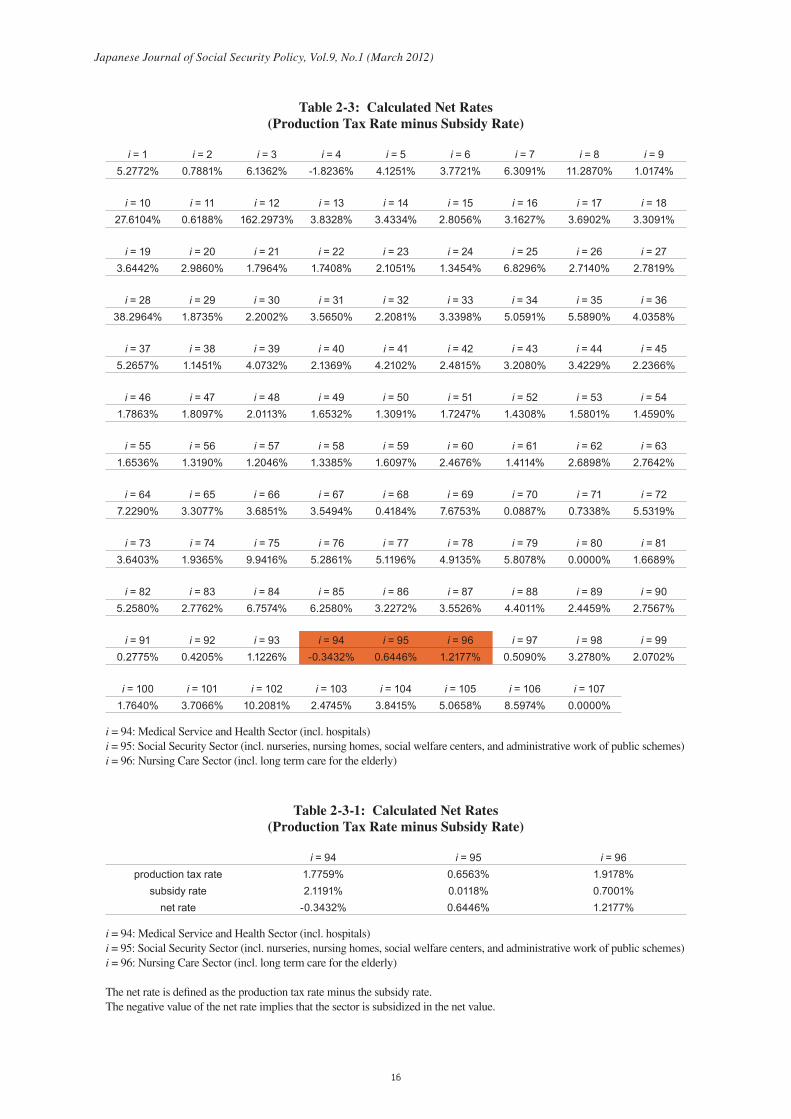
Table 2-3: Calculated Net Rates(Production Tax Rate minus Subsidy Rate)

i = 1 i = 2 i = 3 i = 4 i = 5 i = 6 i = 7 i = 8 i = 95.2772% 0.7881% 6.1362% -1.8236% 4.1251% 3.7721% 6.3091% 11.2870% 1.0174%

i = 10 i = 11 i = 12 i = 13 i = 14 i = 15 i = 16 i = 17 i = 1827.6104% 0.6188% 162.2973% 3.8328% 3.4334% 2.8056% 3.1627% 3.6902% 3.3091%

i = 19 i = 20 i = 21 i = 22 i = 23 i = 24 i = 25 i = 26 i = 273.6442% 2.9860% 1.7964% 1.7408% 2.1051% 1.3454% 6.8296% 2.7140% 2.7819%

i = 28 i = 29 i = 30 i = 31 i = 32 i = 33 i = 34 i = 35 i = 3638.2964% 1.8735% 2.2002% 3.5650% 2.2081% 3.3398% 5.0591% 5.5890% 4.0358%

i = 37 i = 38 i = 39 i = 40 i = 41 i = 42 i = 43 i = 44 i = 455.2657% 1.1451% 4.0732% 2.1369% 4.2102% 2.4815% 3.2080% 3.4229% 2.2366%

i = 46 i = 47 i = 48 i = 49 i = 50 i = 51 i = 52 i = 53 i = 541.7863% 1.8097% 2.0113% 1.6532% 1.3091% 1.7247% 1.4308% 1.5801% 1.4590%

i = 55 i = 56 i = 57 i = 58 i = 59 i = 60 i = 61 i = 62 i = 631.6536% 1.3190% 1.2046% 1.3385% 1.6097% 2.4676% 1.4114% 2.6898% 2.7642%

i = 64 i = 65 i = 66 i = 67 i = 68 i = 69 i = 70 i = 71 i = 727.2290% 3.3077% 3.6851% 3.5494% 0.4184% 7.6753% 0.0887% 0.7338% 5.5319%

i = 73 i = 74 i = 75 i = 76 i = 77 i = 78 i = 79 i = 80 i = 813.6403% 1.9365% 9.9416% 5.2861% 5.1196% 4.9135% 5.8078% 0.0000% 1.6689%

i = 82 i = 83 i = 84 i = 85 i = 86 i = 87 i = 88 i = 89 i = 905.2580% 2.7762% 6.7574% 6.2580% 3.2272% 3.5526% 4.4011% 2.4459% 2.7567%

i = 91 i = 92 i = 93 i = 94 i = 95 i = 96 i = 97 i = 98 i = 990.2775% 0.4205% 1.1226% -0.3432% 0.6446% 1.2177% 0.5090% 3.2780% 2.0702%

i = 100 i = 101 i = 102 i = 103 i = 104 i = 105 i = 106 i = 1071.7640% 3.7066% 10.2081% 2.4745% 3.8415% 5.0658% 8.5974% 0.0000%


Table 2-3-1: Calculated Net Rates(Production Tax Rate minus Subsidy Rate)

i = 94 i = 95 i = 96production tax rate 1.7759% 0.6563% 1.9178%

subsidy rate 2.1191% 0.0118% 0.7001%net rate -0.3432% 0.6446% 1.2177%


The net rate is defined as the production tax rate minus the subsidy rate.The negative value of the net rate implies that the sector is subsidized in the net value.


16

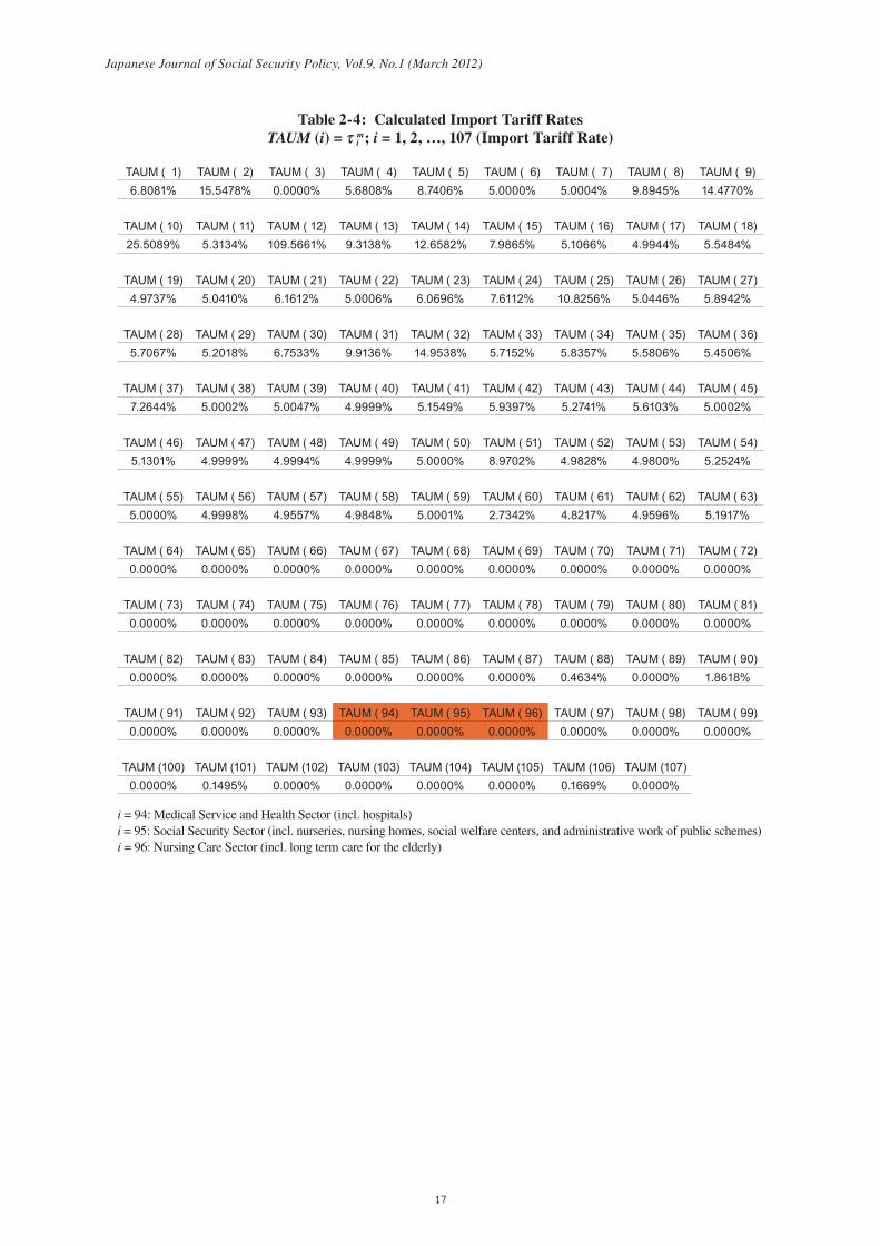
Table 2-4: Calculated Import Tariff RatesTAUM (i) = τ im; i = 1, 2, …, 107 (Import Tariff Rate)

TAUM ( 1) TAUM ( 2) TAUM ( 3) TAUM ( 4) TAUM ( 5) TAUM ( 6) TAUM ( 7) TAUM ( 8) TAUM ( 9)6.8081% 15.5478% 0.0000% 5.6808% 8.7406% 5.0000% 5.0004% 9.8945% 14.4770%











TAUM (100) TAUM (101) TAUM (102) TAUM (103) TAUM (104) TAUM (105) TAUM (106) TAUM (107)0.0000% 0.1495% 0.0000% 0.0000% 0.0000% 0.0000% 0.1669% 0.0000%



17

Table 3-1: Welfare Changes and Government Deficits in Scenario I without balanced budget

Unit: One million Japanese yenChanges from the current level by

No Change 50% decrease 30% decrease 10% decrease 5% decrease

Sec

tors

of t

he P

olic

y C

hang

e

i = 94Hospital Services

Level of Net Rate -0.3430% -0.5145% -0.4459% -0.3773% -0.3602%

EV 0.0000 72,324.9558 43,320.3350 14,358.9275 7,124.9091

Government Deficits 0.0000 5,575.5926 3,391.4450 1,193.5028 642.2169

i = 95Social Welfare

Services

Level of Net Rate 0.6445% 0.3223% 0.4512% 0.5801% 0.6123%

EV 0.0000 23,907.6071 14,283.1010 4,683.3031 2,288.8036

Government Deficits 0.0000 1,858.7765 1,154.6368 446.4262 2.6740

i = 96Long-term Care

Services

Level of Net Rate 1.2177% 0.6089% 0.8524% 1.0959% 1.1568%

EV 0.0000 43,349.2401 25,904.0652 8,542.7766 4,215.3597

Government Deficits 0.0000 3,308.7305 2,031.2598 740.5164 415.8710

No Change 5% increase 10% increase 30% increase 50% increase

Sec

tors

of t

he P

olic

y C

hang

e


Level of Net Rate -0.3430% -0.3259% -0.3087% -0.2401% -0.1715%

EV 0.0000 -7,122.4607 -14,347.9576 -43,224.0817 -72,058.8886

Government Deficits 0.0000 -642.8764 -1,197.1323 -3,422.1261 -5,659.5404


Services

Level of Net Rate 0.6445% 0.6767% 0.7090% 0.8379% 0.9668%

EV 0.0000 -2,286.8033 -4,677.0281 -14,226.5194 -23,750.3989

Government Deficits 0.0000 -268.0347 -447.5516 -1,164.7836 -1,887.0301


Services

Level of Net Rate 1.2177% 1.2786% 1.3395% 1.5830% 1.8266%

EV 0.0000 -4,210.2109 -8,522.1494 -25,715.9784 -42,827.4288

Government Deficits 0.0000 -416.6577 -743.6905 -2,062.0392 -3,393.6230


18

Table 3-2: Welfare Changes in Scenario II with balanced budget

Unit: One million Japanese yenChanges from the current level by

The Initial Sector The Secondary Sector No Change 50%

decrease30%

decrease10%

decrease5%

decreasei = 94

Hospital ServicesLevel of Net Rate -0.3430% -0.5145% -0.4459% -0.3773% -0.3602%


i = 95Social Welfare Services EV 0.0000 2423.5141 1,309.6103 1,118.9443 1,213.9380

i = 96Long-term Care Services EV 0.0000 3246.7760 1,829.1769 1,291.9113 1,293.1866


Services

Level of Net Rate 0.6445% 0.3223% 0.4512% 0.5801% 0.6123%

i = 94Hospital Services EV 0.0000 2281.5951 1833.4901 1472.8157 1352.1648

i = 95Social Welfare Services

i = 96Long-term Care Services EV 0.0000 2158.1755 1,725.3315 1,433.2618 1,335.0303


Services

Level of Net Rate 1.2177% 0.6089% 0.8524% 1.0959% 1.1568%

i = 94Hospital Services EV 0.0000 2914.0142 2,042.8615 1,496.7929 1,401.9186

i = 95Social Welfare Services EV 0.0000 2415.5614 1,612.7331 1,324.7827 1,325.2900

i = 96Long-term Care Services

Changes from the current level byThe Initial

Sector The Secondary Sector No Change 5% increase

10% increase

30% increase

50% increase


Level of Net Rate -0.3430% -0.3259% -0.3087% -0.2401% -0.1715%


i = 95Social Welfare Services EV 0.0000 -1,165.917 -897.6839 874.8535 3,776.3527

i = 96Long-term Care Services EV 0.0000 -1,248.378 -1,082.384 244.4483 2,632.1345


Services

Level of Net Rate 0.6445% 0.6767% 0.709% 0.8379% 0.9668%

i = 94Hospital Services EV 0.0000 -1347.323 -1449.459 -1,607.558 -1,646.823

i = 95Social Welfare Services

i = 96Long-term Care Services EV 0.0000 -1,329.610 -1,402.244 -1,391.838 -1,202.263


Services

Level of Net Rate 1.2177% 1.2786% 1.3395% 1.5830% 1.8266%

i = 94Hospital Services EV 0.0000 -1,382.471 -1,419.171 -1,311.084 -863.7073

i = 95Social Welfare Services EV 0.0000 -1,300.396 -1,209.075 -499.6253 884.8772

i = 96Long-term Care Services


19

Table 4-1: Total Income When the Net Rate of Hospital Services ( i = 94) Sector is Exogenously Changed (Scenario II)


No Change(-0.3430%)*

50% decrease (-0.5145%)*

30% decrease (-0.4459%)*

10% decrease (-0.3773%)*

5% decrease (-0.3602%)*

The Secondary Sectori = 94

Hospital Servicesi = 95

Social Welfare Services 20,846,651.00 20,883,516.78 20,868,751.96 20,854,027.85 20,850,353.13

i = 95Social Welfare Services 4,690,730.00 4,646,766.45 4,664,250.61 4,682,302.62 4,686,903.79

i = 96Long-term Care Services 4,623,554.00 4,623,560.38 4,623,557.78 4,623,557.34 4,623,557.56




Services4,690,730.00 4,690,780.65 4,690,758.84 4,690,750.58 4,690,750.60


Relative Changes (%)i = 94


Social Welfare Services 0.0000% 0.1768% 0.1060% 0.0354% 0.0178%

i = 95Social Welfare Services 0.0000% -0.9372% -0.5645% -0.1797% -0.0816%

i = 96Long-term Care Services 0.0000% 0.0001% 0.0001% 0.0001% 0.0001%



i = 95Social Welfare Services 0.0000% 0.0011% 0.0006% 0.0004% 0.0004%

i = 96Long-term Care Services 0.0000% -0.9648% -0.5807% -0.1849% -0.0842%


5% increase (-0.3259%)*

10% increase(-0.3087%)*

30% increase(-0.2401%)*

50% increase(-0.1715%)*



Social Welfare Services 20,846,651.00 20,842,951.20 20,839,284.11 20,824,643.69 20,810,048.13

i = 95Social Welfare Services 4,690,730.00 4,694,585.49 4,699,293.22 4,718,556.31 4,738,519.88





Services4,690,730.00 4,690,710.09 4,690,712.64 4,690,733.05 4,690,769.77


Relative Changes (%)i = 94


Social Welfare Services -0.0177% -0.0353% -0.1056% -0.1756% 0.0178%

i = 95Social Welfare Services 0.0822% 0.1826% 0.5932% 1.0188% -0.0816%

i = 96Long-term Care Services -0.0001% -0.0001% 0.0000% 0.0002% 0.0001%


i = 96Long-term Care Services -0.0177% -0.0353% -0.1055% -0.1755% 0.0177%

i = 95Social Welfare Services -0.0004% -0.0004% 0.0001% 0.0008% 0.0004%

i = 96Long-term Care Services 0.0847% 0.1877% 0.6084% 1.0434% -0.0842%

*) The level of the net rate of Hospital Service Sector (i = 94)


20

Table 4-2: Endogenous Net Rates When the Net Rate of Hospital Services ( i = 94) Sector is Exogenously Changed (Scenario II)


50% decrease (-0.5145%)*

30% decrease (-0.4459%)*

10% decrease (-0.3773%)*

5% decrease (-0.3602%)*


Social Welfare Services 0.6446% 1.5976% 1.2164% 0.8261% 0.7272%


i = 95Social Welfare Services 0.0000% 147.8545% 88.7127% 28.1626% 12.8113%



5% increase (-0.3259%)*

10% increase(-0.3087%)*

30% increase(-0.2401%)*

50% increase(-0.1715%)*


Social Welfare Services 0.6446% 0.561519% 0.460865% 0.051324% -0.369249%


i = 95Social Welfare Services 0.0000% -12.8853% -28.5009% -92.0376% -157.2857%

i = 96Long-term Care Services 0.0000% -7.0446% -15.5790% -50.2677% -85.8247%

*) The level of the net rate of Hospital Service Sector (i = 94)

Table 5: Welfare Changes in Scenario III with balanced budget and compensation


Changes in the Net Rate of i = 94 from the Current Level byNo Change 5% increase 10% increase 30% increase 50% increase

Level of Net Rate of i = 94 -0.3430% -0.3259% -0.3087% -0.2401% -0.1715%EV 0.0000 1053.2306 2200.9788 6581.5326 11153.1617

Lump-Sum Transfers to i = 94 0.0000 3651.9486 7301.1207 21889.4770 36453.1860 Endogenous Net Rate of i = 95 0.644574% 0.590619% 0.535496% 0.318110% 0.099000%

Relative changes in the endogenous net rate of i = 950.0000% -8.3706% -16.9225% -50.6480% -84.6410%


21

Figure 2:

Utility of the household

Xsi : all other finaldomestic goods consumed by the household

Qi : Output of the

final domestic good i

Xi : final domestic good of i consumed by the household

Xgi : final domestic good of i consumed by the goverment

Imported goods Di : Final Domestic Goods

Zi : domestic production

Yi : Production of Composite Goods

Ki , Li

Exported Goods

Xsi : final domestic good of i consumed by the investment company

ΣjXi,j

:

Intermediate goods

Step 4

Equilibrium Condition

Step 3

Step 1

Step 2


22

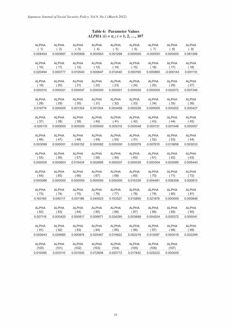
Table 6: Parameter ValuesALPHA (i) = α i ; i = 1, 2, …, 107

ALPHA( 1)

ALPHA( 2)

ALPHA( 3)

ALPHA( 4)

ALPHA( 5)

ALPHA( 6)

ALPHA( 7)

ALPHA( 8)

ALPHA( 9)

0.008454 0.000697 0.000958 0.000563 0.001298 0.000000 -0.000051 0.000000 0.061399

ALPHA( 10)

ALPHA( 11)

ALPHA( 12)

ALPHA( 13)

ALPHA( 14)

ALPHA( 15)

ALPHA( 16)

ALPHA( 17)

ALPHA( 18)

0.020494 0.000777 0.010540 0.000647 0.012440 0.000165 0.000860 -0.000143 0.001110

ALPHA( 19)

ALPHA( 20)

ALPHA( 21)

ALPHA( 22)

ALPHA( 23)

ALPHA( 24)

ALPHA( 25)

ALPHA( 26)

ALPHA( 27)

0.000310 0.000021 0.000047 0.000000 0.000001 0.000000 0.000000 0.002072 0.007346

ALPHA( 28)

ALPHA( 29)

ALPHA( 30)

ALPHA( 31)

ALPHA( 32)

ALPHA( 33)

ALPHA( 34)

ALPHA( 35)

ALPHA( 36)

0.019774 0.000005 0.001354 0.001304 0.003456 0.000226 0.000005 0.000202 0.000427

ALPHA( 37)

ALPHA( 38)

ALPHA( 39)

ALPHA( 40)

ALPHA( 41)

ALPHA( 42)

ALPHA( 43)

ALPHA( 44)

ALPHA( 45)

-0.000110 0.000000 0.000000 0.000000 0.000315 0.000048 0.000131 0.001049 0.000057

ALPHA( 46)

ALPHA( 47)

ALPHA( 48)

ALPHA( 49)

ALPHA( 50)

ALPHA( 51)

ALPHA( 52)

ALPHA( 53)

ALPHA( 54)

0.000099 0.000001 0.000152 0.000082 0.000000 0.002079 0.007615 0.013658 0.003033

ALPHA( 55)

ALPHA( 56)

ALPHA( 57)

ALPHA( 58)

ALPHA( 59)

ALPHA( 60)

ALPHA( 61)

ALPHA( 62)

ALPHA( 63)

0.000005 0.000803 0.015434 0.002895 0.000037 0.000035 0.000304 0.003085 0.005440

ALPHA( 64)

ALPHA( 65)

ALPHA( 66)

ALPHA( 67)

ALPHA( 68)

ALPHA( 69)

ALPHA( 70)

ALPHA( 71)

ALPHA( 72)

0.000086 0.000000 0.000000 0.000000 0.000000 0.015339 0.004461 0.006358 0.000813

ALPHA( 73)

ALPHA( 74)

ALPHA( 75)

ALPHA( 76)

ALPHA( 77)

ALPHA( 78)

ALPHA( 79)

ALPHA( 80)

ALPHA( 81)

0.163165 0.040117 0.001186 0.040023 0.153327 0.013895 0.021978 0.000000 0.000848

ALPHA( 82)

ALPHA( 83)

ALPHA( 84)

ALPHA( 85)

ALPHA( 86)

ALPHA( 87)

ALPHA( 88)

ALPHA( 89)

ALPHA( 90)

0.007116 0.000420 0.000817 0.006671 0.024290 0.003689 0.004204 0.000372 0.005041

ALPHA( 91)

ALPHA( 92)

ALPHA( 93)

ALPHA( 94)

ALPHA( 95)

ALPHA( 96)

ALPHA( 97)

ALPHA( 98)

ALPHA( 99)

0.002643 0.024685 0.000874 0.025467 0.014922 0.002219 0.013087 0.000018 0.002299

ALPHA(100)

ALPHA(101)

ALPHA(102)

ALPHA(103)

ALPHA(104)

ALPHA(105)

ALPHA(106)

ALPHA(107)

0.010085 0.003110 0.031930 0.072608 0.025772 0.017842 0.025222 0.000000


23

Table 6: Parameter Values (continued)TETA (i) = ; i = 1, 2, …, 107

TETA ( 1) TETA ( 2) TETA ( 3) TETA ( 4) TETA ( 5) TETA ( 6) TETA ( 7) TETA ( 8) TETA ( 9)0.000000 0.000000 0.000000 0.000000 0.000000 0.000000 0.000000 0.000000 0.002854




TETA ( 37) TETA ( 38) TETA ( 39) TETA ( 40) TETA ( 41) TETA ( 42) TETA ( 43) TETA ( 44) TETA ( 45)-0.000231 0.000000 0.000000 0.000000 0.000000 0.000000 0.000007 0.000015 0.000930



TETA ( 64) TETA ( 65) TETA ( 66) TETA ( 67) TETA ( 68) TETA ( 69) TETA ( 70) TETA ( 71) TETA ( 72)0.000000 0.023000 0.000000 0.139914 0.015876 0.000000 0.000000 -0.003126 0.008649


TETA ( 82) TETA ( 83) TETA ( 84) TETA ( 85) TETA ( 86) TETA ( 87) TETA ( 88) TETA ( 89) TETA ( 90)0.000001 0.000009 0.000016 -0.000682 0.000000 0.000000 0.009389 0.000000 0.000312


TETA (100) TETA (101) TETA (102) TETA (103) TETA (104) TETA (105) TETA (106) TETA (107)0.000000 0.004877 0.000000 0.000000 0.000000 0.000000 0.000000 0.000000


24

Table 6: Parameter Values (continued)AY (i) = ayi ; i = 1, 2, …, 107

AY ( 1) AY ( 2) AY ( 3) AY ( 4) AY ( 5) AY ( 6) AY ( 7) AY ( 8) AY ( 9)0.569112 0.259441 0.638091 0.714903 0.545627 0.502516 0.372137 0.509977 0.288914











AY (100) AY (101) AY (102) AY (103) AY (104) AY (105) AY (106) AY (107)0.361597 0.735262 0.631194 0.439779 0.470239 0.717599 0.399887 0.000000


25

Table 6: Parameter Values (continued)GSAI (i) = ; i = 1, 2, …, 107

GSAI ( 1) GSAI ( 2) GSAI ( 3) GSAI ( 4) GSAI ( 5) GSAI ( 6) GSAI ( 7) GSAI ( 8) GSAI ( 9)0.000418 0.001846 0.000000 0.007704 0.000023 0.000009 0.000378 -0.001540 0.001904

GSAI ( 10) GSAI ( 11) GSAI ( 12) GSAI ( 13) GSAI ( 14) GSAI ( 15) GSAI ( 16) GSAI ( 17) GSAI ( 18)0.001241 0.000105 -0.000541 0.000953 0.001007 0.001002 0.003683 0.000401 -0.000053

GSAI ( 19) GSAI ( 20) GSAI ( 21) GSAI ( 22) GSAI ( 23) GSAI ( 24) GSAI ( 25) GSAI ( 26) GSAI ( 27)0.000015 0.000003 0.000119 -0.000029 0.000609 0.000388 -0.000063 -0.000118 0.000100

GSAI ( 28) GSAI ( 29) GSAI ( 30) GSAI ( 31) GSAI ( 32) GSAI ( 33) GSAI ( 34) GSAI ( 35) GSAI ( 36)-0.001943 0.000210 0.000776 0.000078 -0.000038 0.000057 0.000003 0.000154 0.000419

GSAI ( 37) GSAI ( 38) GSAI ( 39) GSAI ( 40) GSAI ( 41) GSAI ( 42) GSAI ( 43) GSAI ( 44) GSAI ( 45)-0.001777 0.002139 0.000111 0.000180 -0.001248 0.002241 0.000520 0.003091 0.041242

GSAI ( 46) GSAI ( 47) GSAI ( 48) GSAI ( 49) GSAI ( 50) GSAI ( 51) GSAI ( 52) GSAI ( 53) GSAI ( 54)0.071786 0.018354 0.029925 0.024607 0.015242 0.002979 0.002122 0.019012 0.032610

GSAI ( 55) GSAI ( 56) GSAI ( 57) GSAI ( 58) GSAI ( 59) GSAI ( 60) GSAI ( 61) GSAI ( 62) GSAI ( 63)0.000412 -0.000317 0.035209 0.019425 0.001465 0.002726 0.014186 0.018706 0.011439





GSAI (100) GSAI (101) GSAI (102) GSAI (103) GSAI (104) GSAI (105) GSAI (106) GSAI (107)0.000000 0.024440 0.000000 0.000000 0.000000 0.000000 0.000000 0.000000


26

Table 6: Parameter Values (continued)GAMMAM (i) = γ i

M ; i = 1, 2, …, 107

GAMMAM( 1)

GAMMAM( 2)

GAMMAM( 3)

GAMMAM( 4)

GAMMAM( 5)

GAMMAM( 6)

GAMMAM( 7)

GAMMAM( 8)

GAMMAM( 9)

0.204213 0.015883 0.000000 0.159696 0.169359 0.989016 0.161561 0.991011 0.151897

GAMMAM( 10)

GAMMAM( 11)

GAMMAM( 12)

GAMMAM( 13)

GAMMAM( 14)

GAMMAM( 15)

GAMMAM( 16)

GAMMAM( 17)

GAMMAM( 18)

0.057352 0.092149 0.244285 0.205769 0.588887 0.296517 0.178307 0.078185 0.031427

GAMMAM( 19)

GAMMAM( 20)

GAMMAM( 21)

GAMMAM( 22)

GAMMAM( 23)

GAMMAM( 24)

GAMMAM( 25)

GAMMAM( 26)

GAMMAM( 27)

0.007000 0.228893 0.166364 0.015279 0.262157 0.150654 0.139844 0.130729 0.132632

GAMMAM( 28)

GAMMAM( 29)

GAMMAM( 30)

GAMMAM( 31)

GAMMAM( 32)

GAMMAM( 33)

GAMMAM( 34)

GAMMAM( 35)

GAMMAM( 36)

0.151774 0.065853 0.059744 0.174788 0.634839 0.133737 0.005358 0.134695 0.126247

GAMMAM( 37)

GAMMAM( 38)

GAMMAM( 39)

GAMMAM( 40)

GAMMAM( 41)

GAMMAM( 42)

GAMMAM( 43)

GAMMAM( 44)

GAMMAM( 45)

0.046285 0.038267 0.010569 0.057458 0.518190 0.143344 0.030947 0.067039 0.090442

GAMMAM( 46)

GAMMAM( 47)

GAMMAM( 48)

GAMMAM( 49)

GAMMAM( 50)

GAMMAM( 51)

GAMMAM( 52)

GAMMAM( 53)

GAMMAM( 54)

0.159450 0.094953 0.057172 0.167955 0.392915 0.159768 0.164382 0.199346 0.671938

GAMMAM( 55)

GAMMAM( 56)

GAMMAM( 57)

GAMMAM( 58)

GAMMAM( 59)

GAMMAM( 60)

GAMMAM( 61)

GAMMAM( 62)

GAMMAM( 63)

0.587932 0.147661 0.120402 0.027670 0.026757 0.039290 0.299314 0.389652 0.289767

GAMMAM( 64)

GAMMAM( 65)

GAMMAM( 66)

GAMMAM( 67)

GAMMAM( 68)

GAMMAM( 69)

GAMMAM( 70)

GAMMAM( 71)

GAMMAM( 72)

0.000000 0.000000 0.000000 0.000000 0.000000 0.000068 0.000063 0.000318 0.000072

GAMMAM( 73)

GAMMAM( 74)

GAMMAM( 75)

GAMMAM( 76)

GAMMAM( 77)

GAMMAM( 78)

GAMMAM( 79)

GAMMAM( 80)

GAMMAM( 81)

0.007164 0.012048 0.000000 0.000123 0.000000 0.030748 0.011163 0.000000 0.453834

GAMMAM( 82)

GAMMAM( 83)

GAMMAM( 84)

GAMMAM( 85)

GAMMAM( 86)

GAMMAM( 87)

GAMMAM( 88)

GAMMAM( 89)

GAMMAM( 90)

0.394777 0.000000 0.000000 0.043256 0.005262 0.000000 0.022020 0.002268 0.031897

GAMMAM( 91)

GAMMAM( 92)

GAMMAM( 93)

GAMMAM( 94)

GAMMAM( 95)

GAMMAM( 96)

GAMMAM( 97)

GAMMAM( 98)

GAMMAM( 99)

0.000000 0.002954 0.042848 0.000056 0.000000 0.000000 0.006711 0.022928 0.002069

GAMMAM(100)

GAMMAM(101)

GAMMAM(102)

GAMMAM(103)

GAMMAM(104)

GAMMAM(105)

GAMMAM(106)

GAMMAM(107)

0.000019 0.026586 0.018407 0.041963 0.220840 0.000424 0.058544 0.000000


27

Table 6: Parameter Values (continued)GAMMAD (i) = γ i

D ; i = 1, 2, …, 107

GAMMAD( 1)

GAMMAD( 2)

GAMMAD( 3)

GAMMAD( 4)

GAMMAD( 5)

GAMMAD( 6)

GAMMAD( 7)

GAMMAD( 8)

GAMMAD( 9)

0.795787 0.984117 1.000000 0.840304 0.830641 0.010984 0.838439 0.008989 0.848103

GAMMAD( 10)

GAMMAD( 11)

GAMMAD( 12)

GAMMAD( 13)

GAMMAD( 14)

GAMMAD( 15)

GAMMAD( 16)

GAMMAD( 17)

GAMMAD( 18)

0.942648 0.907851 0.755715 0.794231 0.411113 0.703483 0.821693 0.921815 0.968573

GAMMAD( 19)

GAMMAD( 20)

GAMMAD( 21)

GAMMAD( 22)

GAMMAD( 23)

GAMMAD( 24)

GAMMAD( 25)

GAMMAD( 26)

GAMMAD( 27)

0.993000 0.771107 0.833636 0.984721 0.737843 0.849346 0.860156 0.869271 0.867368

GAMMAD( 28)

GAMMAD( 29)

GAMMAD( 30)

GAMMAD( 31)

GAMMAD( 32)

GAMMAD( 33)

GAMMAD( 34)

GAMMAD( 35)

GAMMAD( 36)

0.848226 0.934147 0.940256 0.825212 0.365161 0.866263 0.994642 0.865305 0.873753

GAMMAD( 37)

GAMMAD( 38)

GAMMAD( 39)

GAMMAD( 40)

GAMMAD( 41)

GAMMAD( 42)

GAMMAD( 43)

GAMMAD( 44)

GAMMAD( 45)

0.953715 0.961733 0.989431 0.942542 0.481810 0.856656 0.969053 0.932961 0.909558

GAMMAD( 46)

GAMMAD( 47)

GAMMAD( 48)

GAMMAD( 49)

GAMMAD( 50)

GAMMAD( 51)

GAMMAD( 52)

GAMMAD( 53)

GAMMAD( 54)

0.840550 0.905047 0.942828 0.832045 0.607085 0.840232 0.835618 0.800654 0.328062

GAMMAD( 55)

GAMMAD( 56)

GAMMAD( 57)

GAMMAD( 58)

GAMMAD( 59)

GAMMAD( 60)

GAMMAD( 61)

GAMMAD( 62)

GAMMAD( 63)

0.412068 0.852339 0.879598 0.972330 0.973243 0.960710 0.700686 0.610348 0.710233

GAMMAD( 64)

GAMMAD( 65)

GAMMAD( 66)

GAMMAD( 67)

GAMMAD( 68)

GAMMAD( 69)

GAMMAD( 70)

GAMMAD( 71)

GAMMAD( 72)

1.000000 1.000000 1.000000 1.000000 1.000000 0.999932 0.999937 0.999682 0.999928

GAMMAD( 73)

GAMMAD( 74)

GAMMAD( 75)

GAMMAD( 76)

GAMMAD( 77)

GAMMAD( 78)

GAMMAD( 79)

GAMMAD( 80)

GAMMAD( 81)

0.992836 0.987952 1.000000 0.999877 1.000000 0.969252 0.988837 1.000000 0.546166

GAMMAD( 82)

GAMMAD( 83)

GAMMAD( 84)

GAMMAD( 85)

GAMMAD( 86)

GAMMAD( 87)

GAMMAD( 88)

GAMMAD( 89)

GAMMAD( 90)

0.605223 1.000000 1.000000 0.956744 0.994738 1.000000 0.977980 0.997732 0.968103

GAMMAD( 91)

GAMMAD( 92)

GAMMAD( 93)

GAMMAD( 94)

GAMMAD( 95)

GAMMAD( 96)

GAMMAD( 97)

GAMMAD( 98)

GAMMAD( 99)

1.000000 0.997046 0.957152 0.999944 1.000000 1.000000 0.993289 0.977072 0.997931

GAMMAD(100)

GAMMAD(101)

GAMMAD(102)

GAMMAD(103)

GAMMAD(104)

GAMMAD(105)

GAMMAD(106)

GAMMAD(107)

0.999981 0.973414 0.981593 0.958037 0.779160 0.999576 0.941456 1.000000


28

Table 6: Parameter Values (continued)KAPPAE (i) = κ i

E ; i = 1, 2, …, 107

KAPPAE( 1)

KAPPAE( 2)

KAPPAE( 3)

KAPPAE( 4)

KAPPAE( 5)

KAPPAE( 6)

KAPPAE( 7)

KAPPAE( 8)

KAPPAE( 9)

0.003039 0.000270 0.000000 0.001252 0.025258 0.182150 0.031150 0.001016 0.008845

KAPPAE( 10)

KAPPAE( 11)

KAPPAE( 12)

KAPPAE( 13)

KAPPAE( 14)

KAPPAE( 15)

KAPPAE( 16)

KAPPAE( 17)

KAPPAE( 18)

0.002643 0.003551 0.010760 0.236228 0.021328 0.004348 0.027498 0.049164 0.015724

KAPPAE( 19)

KAPPAE( 20)

KAPPAE( 21)

KAPPAE( 22)

KAPPAE( 23)

KAPPAE( 24)

KAPPAE( 25)

KAPPAE( 26)

KAPPAE( 27)

0.007009 0.032443 0.137034 0.109029 0.301676 0.290771 0.275001 0.046991 0.193032

KAPPAE( 28)

KAPPAE( 29)

KAPPAE( 30)

KAPPAE( 31)

KAPPAE( 32)

KAPPAE( 33)

KAPPAE( 34)

KAPPAE( 35)

KAPPAE( 36)

0.053784 0.033542 0.103752 0.236375 0.041396 0.210679 0.008462 0.154667 0.145432

KAPPAE( 37)

KAPPAE( 38)

KAPPAE( 39)

KAPPAE( 40)

KAPPAE( 41)

KAPPAE( 42)

KAPPAE( 43)

KAPPAE( 44)

KAPPAE( 45)

0.016499 0.189440 0.010059 0.004244 0.188856 0.158541 0.006420 0.078360 0.261322

KAPPAE( 46)

KAPPAE( 47)

KAPPAE( 48)

KAPPAE( 49)

KAPPAE( 50)

KAPPAE( 51)

KAPPAE( 52)

KAPPAE( 53)

KAPPAE( 54)

0.374836 0.219185 0.064306 0.322125 0.559810 0.440164 0.079687 0.259846 0.607049

KAPPAE( 55)

KAPPAE( 56)

KAPPAE( 57)

KAPPAE( 58)

KAPPAE( 59)

KAPPAE( 60)

KAPPAE( 61)

KAPPAE( 62)

KAPPAE( 63)

0.679630 0.256909 0.527340 0.354772 0.139857 0.604501 0.222479 0.375409 0.139016

KAPPAE( 64)

KAPPAE( 65)

KAPPAE( 66)

KAPPAE( 67)

KAPPAE( 68)

KAPPAE( 69)

KAPPAE( 70)

KAPPAE( 71)

KAPPAE( 72)

0.255331 0.000000 0.000000 0.000000 0.000000 0.001922 0.000244 0.002235 0.000838

KAPPAE( 73)

KAPPAE( 74)

KAPPAE( 75)

KAPPAE( 76)

KAPPAE( 77)

KAPPAE( 78)

KAPPAE( 79)

KAPPAE( 80)

KAPPAE( 81)

0.081116 0.015740 0.000207 0.001465 0.000000 0.015210 0.054490 0.000000 0.619934

KAPPAE( 82)

KAPPAE( 83)

KAPPAE( 84)

KAPPAE( 85)

KAPPAE( 86)

KAPPAE( 87)

KAPPAE( 88)

KAPPAE( 89)

KAPPAE( 90)

0.258458 0.070603 0.049171 0.088519 0.004668 0.000010 0.010135 0.003421 0.010506

KAPPAE( 91)

KAPPAE( 92)

KAPPAE( 93)

KAPPAE( 94)

KAPPAE( 95)

KAPPAE( 96)

KAPPAE( 97)

KAPPAE( 98)

KAPPAE( 99)

0.000000 0.001252 0.027012 0.000006 0.000000 0.000000 0.003981 0.013002 0.012756

KAPPAE(100)

KAPPAE(101)

KAPPAE(102)

KAPPAE(103)

KAPPAE(104)

KAPPAE(105)

KAPPAE(106)

KAPPAE(107)

0.000177 0.013158 0.008165 0.011575 0.088229 0.000147 0.008925 0.000000


29

Table 6: Parameter Values (continued)KAPPAD (i) = κ i

E ; i = 1, 2, …, 107

KAPPAD( 1)

KAPPAD( 2)

KAPPAD( 3)

KAPPAD( 4)

KAPPAD( 5)

KAPPAD( 6)

KAPPAD( 7)

KAPPAD( 8)

KAPPAD( 9)

0.996961 0.999730 1.000000 0.998748 0.974742 0.817850 0.968850 0.998984 0.991155

KAPPAD( 10)

KAPPAD( 11)

KAPPAD( 12)

KAPPAD( 13)

KAPPAD( 14)

KAPPAD( 15)

KAPPAD( 16)

KAPPAD( 17)

KAPPAD( 18)

0.997357 0.996449 0.989240 0.763772 0.978672 0.995652 0.972502 0.950836 0.984276

KAPPAD( 19)

KAPPAD( 20)

KAPPAD( 21)

KAPPAD( 22)

KAPPAD( 23)

KAPPAD( 24)

KAPPAD( 25)

KAPPAD( 26)

KAPPAD( 27)

0.992991 0.967557 0.862966 0.890971 0.698324 0.709229 0.724999 0.953009 0.806968

KAPPAD( 28)

KAPPAD( 29)

KAPPAD( 30)

KAPPAD( 31)

KAPPAD( 32)

KAPPAD( 33)

KAPPAD( 34)

KAPPAD( 35)

KAPPAD( 36)

0.946216 0.966458 0.896248 0.763625 0.958604 0.789321 0.991538 0.845333 0.854568

KAPPAD( 37)

KAPPAD( 38)

KAPPAD( 39)

KAPPAD( 40)

KAPPAD( 41)

KAPPAD( 42)

KAPPAD( 43)

KAPPAD( 44)

KAPPAD( 45)

0.983501 0.810560 0.989941 0.995756 0.811144 0.841459 0.993580 0.921640 0.738678

KAPPAD( 46)

KAPPAD( 47)

KAPPAD( 48)

KAPPAD( 49)

KAPPAD( 50)

KAPPAD( 51)

KAPPAD( 52)

KAPPAD( 53)

KAPPAD( 54)

0.625164 0.780815 0.935694 0.677875 0.440190 0.559836 0.920313 0.740154 0.392951

KAPPAD( 55)

KAPPAD( 56)

KAPPAD( 57)

KAPPAD( 58)

KAPPAD( 59)

KAPPAD( 60)

KAPPAD( 61)

KAPPAD( 62)

KAPPAD( 63)

0.320370 0.743091 0.472660 0.645228 0.860143 0.395499 0.777521 0.624591 0.860984

KAPPAD( 64)

KAPPAD( 65)

KAPPAD( 66)

KAPPAD( 67)

KAPPAD( 68)

KAPPAD( 69)

KAPPAD( 70)

KAPPAD( 71)

KAPPAD( 72)

0.744669 1.000000 1.000000 1.000000 1.000000 0.998078 0.999756 0.997765 0.999162

KAPPAD( 73)

KAPPAD( 74)

KAPPAD( 75)

KAPPAD( 76)

KAPPAD( 77)

KAPPAD( 78)

KAPPAD( 79)

KAPPAD( 80)

KAPPAD( 81)

0.918884 0.984260 0.999793 0.998535 1.000000 0.984790 0.945510 1.000000 0.380066

KAPPAD( 82)

KAPPAD( 83)

KAPPAD( 84)

KAPPAD( 85)

KAPPAD( 86)

KAPPAD( 87)

KAPPAD( 88)

KAPPAD( 89)

KAPPAD( 90)

0.741542 0.929397 0.950829 0.911481 0.995332 0.999990 0.989865 0.996579 0.989494

KAPPAD( 91)

KAPPAD( 92)

KAPPAD( 93)

KAPPAD( 94)

KAPPAD( 95)

KAPPAD( 96)

KAPPAD( 97)

KAPPAD( 98)

KAPPAD( 99)

1.000000 0.998748 0.972988 0.999994 1.000000 1.000000 0.996019 0.986998 0.987244

KAPPAD(100)

KAPPAD(101)

KAPPAD(102)

KAPPAD(103)

KAPPAD(104)

KAPPAD(105)

KAPPAD(106)

KAPPAD(107)

0.999823 0.986842 0.991835 0.988425 0.911771 0.999853 0.991075 1.000000


30

Table 6: Parameter Values (continued)BETA (i, j) = β j

i; i = 1 (capital), 2 (labor), j = 1, 2, …, 107

BETA ( 11) BETA ( 21) BETA ( 12) BETA ( 22) BETA ( 13) BETA ( 23) BETA ( 14) BETA ( 24) BETA ( 15)0.873705 0.126295 0.795029 0.204971 0.377652 0.622348 0.789692 0.210308 0.619845



















31





BETA (1100) BETA (2100) BETA (1101) BETA (2101) BETA (1102) BETA (2102) BETA (1103) BETA (2103) BETA (1104)0.169821 0.830179 0.276521 0.723479 0.565949 0.434051 0.278234 0.721766 0.365413

BETA (2104) BETA (1105) BETA (2105) BETA (1106) BETA (2106) BETA (1107) BETA (2107)0.634587 0.456596 0.543404 0.347163 0.652837 0.000000 0.000000


32

ryuta ray kato - ipss.go.jp

Documents