LEDAS, Ltd.

S. Preis, N. Snytnikov, D. Ushakov

COLLABORATIVE DESIGN-2 (LCS): CONCEPT, ARCHITECTURE, AND COMPUTATION METHODS

Preprint 8

Novosibirsk, 2004

This paper focuses on the problem of collaborative design and approaches to

its solution. A precise statement of the problem is given; possibilities for using additional information to simplify the solution are described. The presentation emphasizes a general architecture of a solver for collaborative design problems. A number of techniques taking into account additional information in order to reduce the distributed problem to the local problem and solve the latter (approximate) problem are described.

This series of preprints is published by LEDAS, Ltd., a Russian company developing and marketing intelligent software solutions.

6, Prospekt Lavrentieva, Novosibirsk, Russia 630090. http://ledas.comemail: info@ledas.com

INTRODUCTION

This document describes the architecture and computation methods developed in the second phase of the collaborative design project. At the very beginning of this phase (August 2003), new objectives were defined, statement of the problem was clarified, and the work on design and implementation of a new product, LCS (LEDAS Collaborative Solver) began. The paper contains everything relevant for the LCS project: problem statement and analysis, goals of the project, architecture and protocols, computation methods (including the results of prototype development and testing).

ACKNOWLEDGEMENTS

The authors are grateful to Vladimir Sidorov, Alexei Ershov, Yevgeny Rukoleev (LEDAS), Arnaud Ribadeau-Dumas and Vitali Telerman (Dassault Systemes, Suresnes, France), who reviewed the results presented in the paper, helped to analyze them and offered valuable advice at all steps of its preparation. Invaluable help from Elena Semukhina allowed us to make the presentation of the material more clear compared to what the authors produced in the first version.

1. COLLABORATIVE DESIGN: GENERAL DEFINITIONS

The term “collaborative design” usually refers to a team of engineers who are

jointly working on the same product. Each of the participants may be responsible either for a certain part or component (e.g., body, wheel, engine, etc.) or for an aspect of the product (economics, design, technology of manufacturing, etc.). In any case each of the participants defines certain constraints on the parameters of the product, and these constraints should not contradict the constraints imposed on the product by the other participants. The ultimate goal is to engineer the product so as to satisfy the final constraints from all the participants.

Two main methodologies for collaborative design have been identified: point-based, when the parties exchange exact values of design parameters, and set-based, when the parties exchange sets of acceptable parameter values. Following many researchers and practical implementers, we believe the second approach to be more promising: the use of sets rather than exact values allows

3

one to cover the entire range of alternative options and process it efficiently by refining the requirements and thus gradually restricting the domain of allowed values. Eventually the process should converge almost monotonically to the final project that satisfies all the parties. In the point-based method, the convergence a generally acceptable variant is not monotone, and its success largely depends on the strategy used to achieve agreement between the parties, while a loss of alternatives may force reconsidering the entire project, even at the last stages of the process.

1.1 Problem statement

Each of the parties in a collaborative design project has their own vision of the product, consisting of a parametric model, possibly with a certain geometry, and of a set of constraints imposed on the model; we call this a local model. In order for the interaction to take place, some parameters of the local model of each party should be parameters of the local model of another party at the same time. These parameters will be called shared, or public. In addition, each of the parties has parameters and constraints that are not visible to other parties; these parameters and constraints will be called local. The objective of collaborative design is to find a combination of values for all the parameters that satisfies all the constraints in the local models. Moreover, some of the constraints can be optional, for optimization only, and so collaborative design most often becomes the problem of optimizing a certain target function related to the optional local constraints of the parties.

It is important to understand the dynamic nature of the problem: the design process is iterative, i.e., models are gradually refined through narrowing the intervals of parameter values and imposing additional constraints. The problem of finding an intermediate global solution arises for each of the parties in every iteration of design (i.e., in every iteration of refinement of local models). We assume that the design process is inherently monotone, i.e., the sets of possible values of parameters cannot expand. In particular, this means that removal of constraints is not allowed. In certain cases, however, this requirement may be violated (for example, if inconsistency is discovered). One needs to ensure that this happens as rarely as possible, or at least that it is possible to restore the values of parameters that were generated before imposing the constraint that led to inconsistency.

Information about each party’s model can be used in a search for solutions that is initiated by any of the parties. There are several natural constraints on the interaction protocol:

4

• A certain part of the information about model cannot be transmitted from the computer it is stored in (this may be due to either technical or legal constraints). We will call the closed part of the model a black-box model. Without loss of generality we can assume that any model outside the computer that is performing the calculations is a black-box model, because the open part of a model can be transmitted to any node for calculation. The open part of a model will be called a white-box model. In view of the above, we can assume that all of the white-box models exist in the network and are local to any computation server in the network.

• Not all participants of collaborative design, and so not all of their local models are accessible at an arbitrary time, which can slow down the computation process significantly.

• Computations over local models and transmitting data for them is resource-intensive, but simply accessing every party’s system is a much more resource-intensive procedure.

Previous analysis of the general problem of collaborative design and a number of discussions made it clear that a more precise statement of the problem was necessary. At present, our objective is to construct certain tools to support collaborative design which can solve the following problems: • Specification of local models with support for black-box and white-box

constraints, as well as shared parameters, and unification of local models into a common global model.

• Support for solution search over the global model with the help of black-box models, including interval constraint satisfaction and optimization. At the same time, we need to calculate the bounds for parameter values and guarantee the existence of solutions within these bounds.

• Minimizing the number of switches between calls to different local models, as well as minimizing the calls of “black boxes”, with the possible exception of calls to the model of the party that initiated the calculation: if it had started the calculation, maximal use of its computational capacity should be made in order to find the solution as quickly as possible.

• Identification, localization, and resolution of inconsistencies. The tools should provide indication of violated constraints, their deletion, and restoration of the consistent configuration (preferably without violating monotonicity of the design process).

5

6

1.2 Results of the previous phase

In the previous phase, capabilities of the NemoNext/LeMo1 solver were analyzed in the context of supporting collaborative design [1]. A prototype was implemented providing elementary capabilities for collaborative design using intervals and constraints. This prototype helped to identify the main problems in collaborative design. In particular, the work on this prototype resulted in to the above statement of the problem, where the solution is sought in a common global model. In spite of some problems uncovered, the prototype confirmed that a general-purpose interval constraint solver (NemoNext/LeMo) could provide a foundation for collaborative design.

Another significant result of the previous phase was a model example “barge”. It was consequently improved and used in the analysis of the new computation algorithms developed and implemented in the prototype version of LCS (see Chapter 2).

The discussions and seminars that laid foundation for the current work should also be evaluated as definitely positive. The following section presents the results of problem analysis based on the results of previous work, as well as an interpretation of these results that summarizes possible approaches to the problem of collaborative design.

1.3 Analysis of the problem

Based on the results of prototyping, discussions and analysis, the following definition was proposed for the computational problem of collaborative design.

Interaction is a pair consisting of a set of parties P and a scheme, or protocol, of interaction S. All the contacts between the parties in the interaction are peer-to-peer and do not include data from other parties. However, it is not necessary at all to assume that each party must interact with all the others. Each party has a model that cannot be shared with the others. Their interactions are based on the use of shared parameters included in the local models.

In each iteration of the interaction, one of the parties calculates the state of its model based on the data received from other parties. Here “data” means not only the interval or exact values of shared parameters, but also any other information that is relevant to the models of the other parties and can be obtained from these parties. Our goal is to develop a scheme that takes a minimal number of iterations to achieve global consistency, i.e., a state in which the values of parameters are

1 NemoNext and LeMo solvers are the result of further development of NeMo+, an

environment for solving constraint satisfaction problems created in the Russian Research Institute for Artificial Intelligence [2].

consistent with all of the local models. We propose a number of ways to extend the collections of data that are

transmitted between the parties, aiming to reduce the number of iterations. Let us define them and consequently examine in detail.

EVE Exact Values Exchange. This is the traditional way to achieve consistency; it cannot, however, be used to resolve cyclic dependencies between parameters. Nevertheless, exact values of parameters proposed by one party can be regarded by others as desired and, if other data are available, can assist in faster achievement of consistency.

IVE Interval Values Exchange, examined in detail in [1]. This approach

supports refinement of the domain of possible values for each parameter (through intersection of intervals and their consequent reduction by constraint filtering, see [2]) and, therefore, restriction of the data space for global consistency search.

WBE White-Box Exchange. A party may share a white-box model with the

other parties; integration of these external white-box constraints into other models allows one to reduce the number of conflicts, obtain tighter intervals for possible values of parameters and achieve global consistency faster.

TVE Tabular Values Exchange. Since direct transmission of black-box models

between the parties is not possible, the parties can exchange sets of parameter values satisfying their local models. These sets can be used by the other parties in order to approximate the inaccessible, hidden black-box models and thus to obtain a globally consistent solution.

DVE Derivative Values Exchange, exchanging the values of partial derivatives

of the black-box functions. These values can be used in Newton-type methods to achieve global consistency.

MSE Model Structure Exchange. Information about the graph of functional

dependencies between the parameters of a black-box model can be transmitted to other parties to assist in correct organization of the search of globally consistent solution.

The NemoNext/LeMo solver can naturally support all of the above information exchange types. The methods EVE, IVE, and WBE are supported by the current versions, while the support for TVE, DVE, and MSE is easy to 7

include in the future versions. NemoNext/LeMo is a perfect fast-prototyping tool for the collaborative design project: we can model cooperation between the parties by using various schemes and their combinations in order to select the best one. In what follows, we briefly describe the known problems in each of the approaches.

Exact Values Exchange One pure implementation of this approach is known as point-to-point

design [3]. How can a global solution be found if only local models and their exact solutions are available? Traditional systems for knowledge-based engineering (KBE), based on the use of formulas and rules, can be applied only to the resolution of acyclic dependencies. Resolution of cyclic dependencies requires using complex iterative algorithms in which the number of exchanges between the design parties can be unacceptably large. However, the NemoNext/LeMo solver can process cyclic dependencies more efficiently because of its ability to find a solution that is close to the initial parameter values. Even in this case, of course, we cannot effectively estimate the number of iterations needed to achieve global consistency, but in some cases this method turns out to be quite useful.

Interval Values Exchange The exchange of intervals or more generally of sets of parameter values is

called set-based design. This method was adapted by Toyota for their production needs and to a great extent has ensured their recognized leadership in the quality of products as well as in the reduction of development time for new products [3]. The main advantage of this method is in its acyclic nature: all relations over intervals are multi-directional, i.e., interval values of any parameter may be used to refine, or reduce the intervals for other parameters; thus, every parameter can be regarded both as an input and as an output parameter. Other advantages are as follows: the global process of interval reduction converges to locally consistent sets of values; heuristic search based on subdivision of intervals allows one to find a globally consistent solution; incremental nature of the process supports quick calculation of new intervals when constraints are added or removed; finally, this approach naturally supports various types of parameters (continuous and discrete) and relations over them (logical, arithmetic, tabular, etc.).

However, the exchange of interval values has two serious drawbacks. Firstly, this method is incomplete in the general case, i.e., existence of an exact solution in the reduced intervals is not guaranteed. Secondly, interval reduction for black-

8

box constraints is a complex computational problem (which was nevertheless implemented in the NemoNext/LeMo solver, see [4] and Chapter 3 of this paper). To overcome the second drawback, we can use weak interval reduction, which uses only white-box constraints.

The NemoNext/LeMo solver is a powerful tool for using interval reduction in constraints: it supports a broad range of various types of data and constraints, including black-box constraints, and implements a number of complex algorithms to search for an exact solution. The first phase of the Collaborative Design project aimed to demonstrate these strengths of the solver. In the second phase, we continued the experiments related to the development of new methods of interval reduction for black-box constraints, as well as of new methods for exact solution search.

White-Boxes Exchange The simplest way to improve the quality of collaborative design is to allow

exchange of white-box constraints between the parties. The use of the constraints imposed by one party in the models of the other parties allows one to avoid many conflicts in collaborative design. This approach can be used, for instance, to solve the simple problem examined in [1]. In the general case the exchange of white-box constraints is used along with EVE/IVE. It reduces the probability of EVE producing a solution that will be rejected by one of the parties. However, the addition of white-box constraints of one model to another model can create cyclic dependencies, and so it is appropriate to use NemoNext/LeMo for WBE. For IVE, the use of WBE allows obtaining tighter value intervals than for “pure” IVE. Here again the use of NemoNext/LeMo is justified because this solver naturally supports manipulation of interval values.

Tabular Values Exchange If we have information on the values of a black-box function at several

points, i.e., at the points of a grid constructed in the reduced intervals, we can approximate the black-box function with a white-box function (a polynomial or a spline, see, e.g., the method of Response Surface Approximation [5]). We can reduce the intervals with the help of NemoNext/LeMo by extending the model of one participant with the approximating white-box expressions for the model of another participants, exchange the resulting intervals and construct the grid again with a smaller grid pitch. Continuing this process iteratively, we obtain a global solution satisfying all of the black-box models. Our experimental application of this method is described in the third chapter of this paper.

9

Derivative Values Exchange The use of partial derivatives of black-box functions with respect to the

shared, i.e., public parameters allows us to use first- or second-order gradient methods to search for a globally consistent solution. In this case, we change the current values of the public parameters according to Newton’s corrections, xn+1 = xn – J-1(xn)f (xn), where J-1(x) is the inverse of Jacobi’s matrix at x. Combining iterations of Newton’s method and interval reduction, we can effectively achieve global consistency. The scheme EVE+IVE+DVE requires testing.

Model Structure Exchange Functional dependencies between the parameters of a single model can be

used by another design party to perform heuristic search for a globally consistent solution simultaneously with the use of IVE. For example, if we know that the dependency between the parameters x, y, z and w is of the form f (x, y, z) = w, we can search for an exact solution by subdividing the intervals for the parameters x, y, and z, but not for w. Also, we can obviously use EVE to find the solution that is closest to the current values of the parameters (by utilizing the capabilities of NemoNext/LeMo).

Conclusions Several of the above-mentioned techniques that can be applied to reduce the

number of interactions between the parties during computation are quite promising. Further experiments in order to evaluate their effectiveness are needed. The combinations offering the best possibilities for application are: EVE+IVE+MSE (combined with heuristic algorithms of directed dichotomy) and EVE+IVE+DVE (with a variant of iterative Newton’s method). Both combinations can be effective for problems with black-box constraints due to providing more complete and accurate information about them. WBE is a useful technique that can be used independently of the others and should accelerate convergence due to centralization of the model. All these techniques can be implemented in the NemoNext/LeMo environment. Some experiments of this kind have already been carried out, and the results are presented in Chapter 3. The results presented there apply in fact to the implementation of EVE+IVE+TVE. The other experiments are still to be performed.

10

1.4 Requirements for the interaction network

Apart from its computational part, the problem of collaborative design contains an aspect related to the “infrastructure”—building a distributed computation problem, developing a protocol for its specification, assembling the global model from the local ones, defining the common procedure for the interaction of the design parties over the entire design process, etc. Generally speaking, different processes and protocols for collaborative design are possible. They depend on the specific application, methods and processes used in the organization and on many other factors. However, some general requirements must be set.

Thus, we begin with the following assumptions: • Each of the design parties is the operator of a certain software system that

supports a common network communication protocol for collaborative design. Each party is working independently of the others in its own environment.

• Parties may publish the parameters that they believe to be important for other parties and, respectively, to access the parameters of other parties. Here the word “access” means that the parties may impose constraints on the shared parameters as well as to view and modify the parameters’ values. In order to make the design process monotone, we assume that any modification of a parameter changes either the interval of possible values or the exact value of the parameter; this value is regarded as preferred for the party. In general, it is possible to limit the access, but we are not discussing data security issues in this document. In a certain sense one can assume that each party has its own, local copy of a shared parameter that it can control. All these local copies are linked by the constraints of equality in the global model.

• Each party imposes its own constraints that relate its own local parameters with shared parameters. The constraints are displayed in the global model if the party wishes so. Their presence in the global model means only that they can be used in computations, while the decision on opening the type of constraints, i.e., on presenting them as white boxes, is made by each party separately. Black-box constraints are always computed in the node that has registered them.

• It is allowed in principle to share information about constraints. In other words, the parties may use the constraints published by other parties in their models. This extension does not contradict anything; one can assume that the parameters of such a constraint become public, and the constraint itself becomes a part of the local model of the participant who has published this constraint.

11

• It is allowed in principle to declare constraints to be equal (identical). Constraints that are independent of local parameters can be declared equal and consequently computed locally in each node that has registered the identical constraint. The computation process is not essentially changed by this action: the computation of some constraints may simply become more efficient due to their local use.

• The use of local and remote constraints in computations may differ: the cost of local computations is always lower, and thus the volume of these computations may be greater. Computing a set of values for a constraint in a single request is cheaper than computing just one value, since the cost of switching between different remote nodes or constraints is significantly higher than the cost of a single constraint calculation.

• The state of a local model of a party may be inconsistent. Special measures must be taken in order to remove these local models from the global computation process. They may be disabled totally or individually for each constraint. In the general case, computation in which some constraints are ignored is bad practice and should be avoided.

• For the sake of convenience in the description of computation algorithms we define the notion of a global model, i.e., a virtual entity containing the collection of all local models and the values of all parameters. The global model need not exist permanently—it is assumed that at computation time it exists in the node where the computation is performed.

• Some information from the parties, mostly of descriptive nature, is available after their registration in the global model, i.e., in fact as a result of a meaningful action of the user, while other information, e.g., the values of registered parameters or the values obtained as a result of computing a constraint, can be obtained automatically, transparently for the user, so as not to distract him.

• The computation completes successfully if it is possible to find the values of parameters that make all the current, valid local models consistent. Otherwise inconsistency is reported. Inconsistency may be characterized by the set of constraints that produce it. A minimal set of constraints without which the problem is consistent will be called the source of inconsistency. Such a set of constraints may be non-unique, but any such constraint contains meaningful information for analysis of the situation. Additional meaningful information is the measure of violation of constraints, called discrepancy. For obvious reasons, information about contradictions in constraints can be presented only to their owner.

• Constraints may have priorities. The priority affects the solution sequence for a problem if it is inconsistent: lower-priority constraints are examined last,

12

and so they will lead to inconsistency with higher probability, and the higher their discrepancy. Priorities may be assigned by the parties (as a way to limit access rights) or by the computation environment. Thus, for example, the environment may lower the priority of the constraints belonging to the party that initiates the computation, in order to check consistency of the external model and to simplify diagnostics. In this case, the diagnostic information is more likely to contain information for the initiator of the computation.

1.5 LCS: a solver for collaborative constraint processing

Based on the above, it appears reasonable to develop a specialized software product, a kernel for a collaborative design system. At the upper level, this product could provide the tools for specification of models with constraints, in accordance with the ideas presented above, and organize computations when requested, once the global model has been built. The computation could be optimized for a distributed structure of the model in accordance with 1.3, and its results could produce more accurate values or diagnostic messages with a localized source of inconsistency. The development of such a product is the ultimate goal of the LCS project.

Moreover, the assumptions described above impose no restrictions on the area of their application. Any constraint-based end-user environment that supports distributed operation will most probably satisfy the above conditions both in the protocol and the organization of computation. For instance, considerable attention is presently paid to communication facilities for the solution of planning problems. Our experience shows that the use of constraints for these problems is quite natural, and so it is possible to use a kernel supporting the principles described above not only for collaborative design, but also for collaborative planning. Thus, one can speak of a solver that supports almost any kind of collaborative activity, i.e., collaboration in the general sense.

13

2. ARCHITECTURE OF LCS

The description of architecture given below is a preliminary vision of LCS. Not all of the architectural problems have been resolved, not all of the functionality is clear, and not all aspects of the protocol and API have been worked out. However, this description should allow one to see the outline of the system, evaluate how novel, promising and useful it is. In addition, we hope that the presentation creates an impulse to develop the ideas at the basis of LCS, to elicit comments and suggestions aiming at quick completion of design and a transition to the implementation of the first version of LCS.

2.1 General architecture of the system

It is assumed that LCS will be a collection of modules. It will provide the entire technological and computation-oriented functionality for organization of collaborative work through its programming interface (API). We are not planning to include real network communication tools in LCS, so as not to restrict applications in the selection of protocols. However, we assume that LCS may be embedded in a network environment for demonstration of its capabilities, even though there is another way, through emulation of a distributed environment within one application via direction translation of calls.

In any case, the API will be structured so as to allow simple translation of the corresponding calls from one instance of LCS to another. Thus, LCS requests will possibly be implemented as callbacks, and replies to requests as calls with the signature of the callback. A sample API is presented in section 2.4 below.

Fig. 1 shows the general architecture of LCS. It shows the following modules:

Local Model Manager (LMM) is the module that controls the local model of a party. It registers all of the local constraints used in global computation, as well as its own public parameters. In addition, this module services the requests for computation of local constraints and retrieval of parameter values.

Global Knowledge Manager (GKM) is the module that controls the global model. It provides access to all of the shared objects and access to every specific local constraint in the process of computation. This module responds to all requests related to the global model. It communicates with similar modules of the other parties and forms the virtual, distributed global model that is presented to the node that requests computation as necessary.

Computation Engine (CE) is the module responsible for organization of the computation process. It accumulates the global model, relays it to the solver, and assists the solver during computation, i.e., processes the requests for computation

14

of black-box constraints, gathers initial data and broadcasts the solution. In addition, it is responsible for diagnostics of inconsistencies and ensures independence of the system as a whole from the solver.

Constraint Solver is a general-purpose solver for constraint satisfaction problems. Through the use of advanced mechanisms included in LCS (such as partial constraints, localization of contradictions, etc.) it should provide a broad range of functions. However, we are not committed to a specific solver: it is possible in principle to attach any solver for constraint problems. This attachment is carried out through a special module that translates the representation of the (global) LCS model into the model needed by the solver. In the first phase, it is planned to use NemoNext/LeMo, as a solver that answers the needs of LCS in the best way.

Party 2

Party1

Local Model Manager

App

licat

ion

App

licat

ion

Global model

Global Knowledge Manager

Computation Engine

Constraint solver

Local Model Manager

Global Knowledge Manager

Fig. 1. Architecture of LCS illustrated by an example with two parties

Fig. 1 shows a fragment of a collaborative design system based on LCS. In the system, we have two parties using different configurations. The first party (party1) has the entire collection of LCS modules. It can specify its own local model, use shared parameters in it and share its own parameters with other parties, as well as perform computations of the combined configuration. The second party (party2) does not have the latter capability, for it does not have the computation module.

15

Other configurations are possible as well. For example, an application may contain LMM only. Since the application performs all of the physical interactions, it can send the requests for parameter values and computation values directly to LMM, with no participation of GKM. In this case, the application cannot use external parameters and perform computations, but can participate in the computation through its model and share its parameters.

Another important configuration example is a computation server, i.e., a system without LMM. It has no local model, and all the participants have equal rights, but it can perform computations, which may be its only task.

2.2 Protocol for interaction

In a real computation network, each node can solve several problems simultaneously, and so we need to introduce the notion of a session. We define a session as a computation network (a set of nodes in which each node is connected to every other node) that exists in time and aims to solve one specific problem of collaborative design. Existence in time means that nodes can connect to the network consecutively, establishing all of the required connections and identifying a specific session they belong to. Each session must have an identifier, so that a node could determine the session it belongs to.

Session management In LCS, the notion of a session, as well as the entire distributed nature of the

problem, is concentrated in GKM. Accordingly, all requests to create a new session, search for available sessions, connect to a session, and report information about the current session are addressed to this module. The search for available sessions, like the rest of network communications, is a task for the application, and GKM only responds with the list of sessions it is participating in at the moment. After this information has been gathered for the entire computation network (via polling the list of nodes, broadcasting or any other method), the application can compile the list of all available sessions.

A request for participation in a specific session is processed by each node (GKM) via registration of a participant of this session. Since every node interacts with every other node, this registration should be performed for all the parties in all the nodes of the network that belong to the session. Moreover, the request contains the identifier of the session and the formal interface for sending requests, a structure that contains a description of the party and the request handling methods. If computation is organized within a single programming environment, then methods of other GKM’s in the network can serve as handler methods, and so can the methods of LMM, since it is a full-fledged participant of

16

the network with a locality flag. In a real distributed system, one needs to construct handlers that transmit the requests over the network. In technologies like CORBA, DCOM, or SOAP, these handlers are constructed automatically.

Model management An application transfers its model to LCS by registering its (shared)

parameters and constraints with LMM. GKM can receive this model and consequently broadcast it over the network. The interface for receiving a model is implemented both by LMM and by GKM, which enables any GKM to construct the global model by traversing the list of session participants. Each constraint and parameter is associated with certain description and status information that assists in more efficient organization of the computation process. In addition, each constraint is associated with the function that computes it. The values of parameters are filled in by a direct call from an application, while GKM requests them from other GKM’s or from LMM. Both the application and the GKM must request modified parameter values from LMM.

CE receives the global model from its GKM by means of standard model transmission requests with the global flag set. GKM uses the same requests with the local flag set to receive models from other GKM’s. In those systems where not all of the connections have been established, requests may be identical, while GKM in this case has the responsibility to delete duplicate data. An application can use global requests to query GKM for information on available shared parameters, in order to use them in its constraints.

CE relays computation and data retrieval requests to its GKM, which relays the request to the relevant node.

Propagation of computation results Computation results are broadcasted through the local GKM of the CE that

performed the computation. Upon completion of the computation, CE calls GKM and relays the session status (general computation results), status and discrepancy values for constraints, and new data values. This information is transmitted through the corresponding GKM’s to those nodes of the network for which the parameters and constraints are local.

Locks and rollbacks It is possible that a party modifies the model locally so that it becomes

inconsistent and local constraints cannot be computed correctly. In this case, incorrect constraints must be locked. Since computations without constraints can produce inconsistent results when the constraints are unlocked, the locking

17

mechanism should be designed with special care. In particular, based on the assumption that the model changes in the process of design are largely monotone, once can temporarily declare the parameters occurring in the locked constraints to be constant. In this case, the computations performed after the constraints are unlocked will take into account all of the changes, and if the monotonicity condition has not been violated, the computation will be successful or will lead to inconsistency in unlocked constraints, which is normal.

If inconsistency has been discovered, and its resolution requires deleting a constraint that has been introduced in an internal (not the latest) step, the requirement of monotonous changes will be violated (to be precise, this applies to all similar deletion operations). Deletion of the last constraints imposed does not violate this property, since their effect has not been realized in the solution yet, and so this constraint has not in fact been applied. If the monotonicity property has been violated, a rollback to the parameter values prior to addition of the constraint is necessary. In the general case, this implies rejecting the current solution and performing the computation “from scratch” without the deleted constraints. This is obviously computation-intensive, and so one may need to design a mechanism for saving intermediate states (synchronized with the state of the model) and rollbacks to these states.

2.3 LCS functions and an outline of API

The functionality of LCS matches exactly the needs for specification, computation, and analysis of the results of collaborative design that have been described above.

Session management in GKM NodeID CreateSession(SessionID, NotificationHandler) creates

a new session. This function is always called at the beginning of any work with GKM. The message handler can be passed as the second parameter. It is assumed that GKM can report important events and requests, so that the application can process them. The function returns a unique node ID that can be passed to JoinSession calls by other nodes in the same session. In addition, the same ID will be passed by the application to the JoinSession call of the local GKM during registration of LMM.

JoinSession(SessionID, NodeID, RequestHandler) adds a new party to the session. RequestHandler is a structure that contains handlers for requests from nodes work with the model, as well as descriptive information about the party. This function adds the party to the list of participants of the session specified by the first parameter. 18

LeaveSession(SessionID, NodeID) is the request to remove a node from the session. This operation is not very safe, because it is equivalent to deleting constraints from the model and violates monotonicity. In this case, modifications to the parameters of the deleted node and the parameters of its constraints may need to be locked at the level of GKM.

DestroySession(SessionID) removes a session completely.

Specification of local model in LMM Constraints and objects can be created only in LMM. They are specified by

the application through the corresponding functions. ModelID CreateModel(NodeID) creates an empty local model for the

specified node. NodeID is the value returned by the function CreateSession, and it can be zero if the LMM services only one session.

ParamID AddParameter(ModelID, LocID, ParDescr) – creates a parameter. The function is passed its local identifier and a description in the form of a structure containing at least its type, name, and options. The global ID for the parameter is returned.

ConstrID DefineConstraint(ModelID, LocID, ConstrDescr) creates a constraint. The description ConstrDescr is a large structure that contains the description of its actual or formal parameters, options (such as priority, shareable or not, white-box, external use, synonym, etc.), a number of parameters depending on the options, for instance, the name of a shareable constraint, and the call-back function for calculation.

RemoveConstraint(ConstrID) deletes the constraint from the local model.

LockConstraint(ConstrID, LockSet) locks or unlocks a constraint. Here LockSet is a logical variable that determines whether the constraint is to be locked or unlocked.

LockParameter (ConstrID, LockSet) locks a parameter from changes (makes it a constant). LockSet is a logical variable that determines whether the parameter is to be locked or unlocked.

Model management It has already been pointed out that GKM and LMM implement identical sets

of functions that handle model-related requests. These functions are listed below. The references to these functions are provided in the structure RequestHandler in the call to JoinSession ().

19

ParDescr* GetNextParam(SessionID, ParLookupContext*) iterates over the model’s parameters. ParLookupContext is a structure that contains the filtering options (select all parameters or only local ones, parameter type, status, etc.) and information about the current position of the iterator. It is changed in every access and should be zeroed before the first access. ParDescr* GetNextConstraint(SessionID, CnstrLookupContext*) iterates over the model’s constraints. CnstrLookupContext is a structure that contains the filtering options (select all constraints or only local ones, constraint type, status, etc.) and information about the current position of the iterator. It is changed in every access and should be zeroed before the first access. Value GetParamValue(SessionID, ParamID) retrieves the value of a parameter. Value is a structure that contains both the interval or set value and the exact (desired) value of the parameter. It will possibly contain a mask indicating the fields used. SetParamValue(SessionID, ParamID, Value, override) sets the parameter to a new value. Value is a structure that contains both the interval or set value and the exact (desired) value of the parameter. Override is a logical variable that determines whether the new value should replace the old one or intersect it (in the set/interval sense). CnstrResult CheckConstraint(SessionID, ConstrID, Opts, CnstrValues*) checks (executes, computes) a constraint. The options Opts define the way to compute the constraint: computation with current values of actual parameters can be requested as well as computation with given values or even multiple computations with several sets of parameters. The interpretation of the parameter CnstrValues* and the result depends on the computation options. CnstrStatus GetConstraintStatus(SessionID, ConstrID) retrieves the status of a constraint. The status is based on the computation results and may include the discrepancy of a constraint. SetConstraintStatus(SessionID, ConstrID, CnstrStatus) sets the current status of a constraint. ParStatus GetParamStatus(SessionID, ParamID) retrieves the status of a parameter. The status is based on the computation result, and may contain, in particular, the information on whether the parameter has changed. SetParamStatus(SessionID, ParamID, ParStatus) set the new status of a parameter. WBNode ExploreWhiteBox(SessionID, WBLookupContext*) traverses a white-box constraint. WBLookupContext is a structure containing information about the direction of the current step, options, and the context (should be zeroed before the first step). 20

Start computations CE will have only one method. CalcResult Run(SessionID, RequestHandler): here the local GKM

serves as RequestHandler. In this call, CE assembles the global model, compiles it into a solver model with the black-box calls routed through GKM, and starts the computation. When the computation is complete, the results will be broadcast over the network through GKM.

2.4 Open problems

The engineering work on LCS is not complete yet, and there are a number of unsolved architectural problems. The most challenging of them are listed below. • The problem of locking constraints (in local models). This problem has

already been mentioned: computation without some constraints and subsequent restoration of these constraints violate the monotonicity requirement for the design process, and so are undesirable. It is not quite clear what one can do to avoid contradictions and rollbacks. One solution is to lock the parameters of the locked constraints, but in this case the search for a solution may be hampered due to degradation of the model’s convergence properties.

• So far, we have assumed that special constraints (such as geometry, scheduling constraints, etc.) will be included in the black-box part of the local model. However, this may increase significantly the dimension of the black-box constraints and thus impair computation accuracy and speed. One way to overcome this problem is to provide the ability to embed specialized solvers in CE and to pass specialized constraints and their parameters as white boxes, if desired by the user. However, this creates numerous problems: from the need to allow objects as parameters of constraints (with at least the ability to aggregate them) to the issue of cooperation between solvers.

• Serious problems with diagnosing contradictions in the distributed case. It is quite possible that the source of inconsistency is in the constraints that do not belong to the party that initiated the computation. In this case, one needs to present a clear diagnostic message to this party, as well as to supply the party whose constraints led to the inconsistency with complete diagnostics. The other party may not even know that its constraints were used in the computation. The subsequent procedure for resolution of inconsistencies is also not clear. It appears that this problem should be solved with the help of the application’s other functions, such as message exchange between the parties, etc. Certain support from the solver is possible, which improves the situation somewhat: if the priority of the constraints created by the party that

21

initiates the computation is lowered, this increases the probability that it is the local constraints that are not satisfied, rather than remote ones, which allows the initiator to handle the situation better.

• Interchangeability of solvers is an open issue. In the proposed API, CE collects the model and analyzes it, converting into a model for the solver. Thus, it determines what to take into account in the description of the model. As a result, the use of different solvers will produce different results. This becomes the biggest problem in the case when systems using different solvers are working jointly in one session.

• The implementation and use of mechanisms for constraint sharing and identification in different nodes requires detailed study.

• The issues related to system access rights, both for data and functions, have been completely left out of this document and all the discussions.

• The system of notifications about system events requires detailed study. It can significantly expand the capabilities of an application in controlling and managing collaborative design. In addition, this notification system can provide a foundation for access rights control.

3. COLLABORATIVE DESIGN: INTERPOLATION APPROACH

In this chapter we use the terminology common to constraint programming, as well as the notation and concepts of [6], since the two papers are close connected, both in the ideas and in specific implementations.

We assume that we have a system, called a CP-system, which enables one to solve problems consisting of a collection of constraints; this collection of constraints will be called a model. Moreover, we assume that the CP-system can manipulate a set of black boxes. The following notions refer to their implementation: • A black-box constraint links the parameters and variables of a model. The

analytic form of such a constraint is unknown. In practice, black-box constraints may encapsulate continuous functions, tables, geometric constraints, etc.

• A black-box procedure is a function that is external to the model and implements a black-box constraint.

• A black-box constraint is represented by a programmatic object of the CP system, which implements the constraint in the model.

• A heuristic is the component of a black-box constraint, which is responsible for the transformation of the constraint’s arguments into the arguments of the black-box procedure. In other words, the main task of a heuristic is to implement the interaction between the black-box procedure and the black-box

22

constraint, for instance, so that the latter would be perceived in the CP-system as an ordinary constraint.

• Multiple call of a black-box procedure is associated with passing a certain vector of arguments to the procedure. For instance, it is possible to obtain a thousand values from a black-box procedure via a single transmission of a vector containing 1,000 sets of arguments.

Now we define the main requirements for the computation methods used in collaborative design. • Minimization of the number of black-box calls. We assume that each call of

an external procedure is a very expensive process. • Minimization of the number of switches between calls of black-box

procedures. We assume here that a switch is much more expensive than a call for one set of arguments.

• Closeness of the solution to the exact one. Unfortunately, the methods for working with black boxes obviously do not guarantee existence of a solution for the original problem, unlike, for example, the interval approach. Nevertheless, we assume that it is not desirable either to find an erroneous solution or to lose a solution in the process of computation.

The principal idea of the methods developed in this paper is to interpolate black boxes with the help of analytical functions, such polynomials, splines, etc. Thus, instead of looking for an interval estimate for a black-box function, as it was done in [6], we will deal with a known constraint that approximates the black box. We will demonstrate below that in some cases this approach allows one to reduce the number of calls and switches to black-box procedures without loss of solution quality.

Thus, in our approach the scheme of computation in a CP system is as follows for all of the implemented heuristics: 1. Construct a grid on the domain where the arguments of the black-box

procedure are defined; 2. Call the black-box procedure at all grid points; 3. Based on the series of values thus obtained, approximate the black-box

function with the help of a common interpolation method; 4. Use the algorithm of interval reduction to compute a model in which the

black-box constraint is replaced by the approximating function constructed above.

In the current implementation, the approximating function is computed with the method of interval reduction. This implementation is far from optimal, since the computation of an interval estimate with this method for linear and

23

polynomial functions takes much longer than directly computing the interval estimate for the analytic expressions of approximating polynomials.

In the rest of this chapter we describe the heuristics that have been implemented, omitting some known mathematical facts from interpolation theory, and then examine a model example that demonstrates practical advantages of the approach.

3.1 One-dimensional heuristics

To interpolate a black-box procedure in the case when it is a one-dimensional function f(x), a polynomial interpolation and a spline interpolation were implemented.

Polynomial interpolation (Interpolation)

1. A uniform grid is constructed on the domain of the function. 2. The black-box procedure is called at each grid point. 3. The interpolating polynomial is sought with the help of the method of

indefinite coefficients: the system of linear equations Ax = b is constructed from the grid points and the computed values, and then solved with the Gauss method.

Thus, for N calls of the black-box function we obtain a polynomial of degree N–1.

Spline interpolation (Spline)

1. A uniform grid is constructed on the domain of the function. 2. The black-box procedure is called at each grid point. In addition, derivatives

at the ends are calculated. 3. A cubic spline is constructed for the grid. In the process of construction, a 3-

diagonal system of linear equations is solved.

To obtain the N cubic polynomial for the spline, we need N+3 calls to the black-box function.

Solution search algorithms To find an exact solution that satisfies all constraints of a model, the

following algorithms are proposed (they have been implemented only for spline interpolation).

24

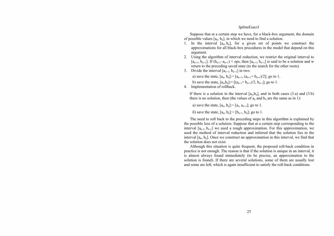
SplineExact1

Suppose that at a certain step we have, for a black-box argument, the domain of possible values [an, bn], in which we need to find a solution. 1. In the interval [an, bn], for a given set of points we construct the

approximations for all black-box procedures in the model that depend on this argument.

2. Using the algorithm of interval reduction, we restrict the original interval to [an+1, bn+1]. If (bn+1–an+1) < eps, then [an+1, bn+1] is said to be a solution and w return to the preceding saved state (to the search for the other roots).

3. Divide the interval [an+1, bn+1] in two: a) save the state, [an, bn]:= [an+1, (an+1+ bn+1)/2]; go to 1. b) save the state, [an,bn]:= [(an+1+ bn+1)/2, bn+1]; go to 1.

4. Implementation of rollback.

If there is a solution in the interval [an,bn], and in both cases (3.a) and (3.b) there is no solution, then (the values of an and bn are the same as in 1):

а) save the state, [an, bn]:= [an, an+1]; go to 1.

б) save the state, [an, bn]:= [bn+1, bn]; go to 1.

The need to roll back to the preceding steps in this algorithm is explained by the possible loss of a solution. Suppose that at a certain step corresponding to the interval [an-1, bn-1] we used a rough approximation. For this approximation, we used the method of interval reduction and inferred that the solution lies in the interval [an, bn]. Once we construct an approximation in this interval, we find that the solution does not exist.

Although this situation is quite frequent, the proposed roll-back condition in practice is not enough. The reason is that if the solution is unique in an interval, it is almost always found immediately (to be precise, an approximation to the solution is found). If there are several solutions, some of them are usually lost and some are left, which is again insufficient to satisfy the roll-back conditions.

25

SplineExact2

Suppose that at a certain step we have an interval [an, bn] in which we must find a solution. 1. In the interval [an, bn], for the given number of points we construct

approximations for all black-box procedures in the model that depend on this argument (it is assumed that at least one black-box procedure is approximated by a spline).

2. The algorithm of interval reduction is used to narrow the original interval to [an+1, bn+1]. If (bn+1–an+1) < eps, then [an+1, bn+1] is called a solution and we go back to the preceding state (the search for the other roots).

3. Since the interval [an, bn] has already been divided into several parts [xi, xi+1] in the computation of the spline at step 1, the new spline is constructed in each interval [xi, xi+1] (even if there were no solution in this interval) by the following rule: a) save the state; [an,bn]:= [xi, (xi+1+xi)/2]; go to 1. b) save the state; [an,bn]:= [(xi+1+xi)/2, xi]; go to 1.

Test results The heuristics have been tested on a number of examples that included black-

box procedures specified via elementary functions, as well as on more complex models that include several black-box procedures and a number of other constraints. In what follows, we consider one such model. The quality of one-dimensional heuristics using the interpolation approach was compared, in accordance with previously defined criteria, with the results of the heuristics implemented in [6] and using a direct interval estimate.

Model example “Barge”

Consider an example in which two engineers are designing a barge. The barge has the shape of a trough: its intersection with the plane z = const is a rectangle, it has a flat bottom, and its bow and stern are rounded. The first engineer can calculate the area of the side surface, while the second can calculate the length of the rounded part.

The goal of collaborative design in this case is calculation of the possible values of parameter k, which is the ratio of the length of the rounded part to the height of the barge. This and the following examples are written in the language of the CP system LeMo.

26

length, width, height, x1, x2, k, BargeVolume, SteelVolume, w_st, S_y :real; x1 = 10*x2; // length of flat part of bottom x2 = 1.0; // length of rounded part along the X coordinate w_st = width*0.01; // wall thickness length = x1 + 2*x2; // barge length width = x2; // barge width height = k*x2; // barge height 0.1 <= k <= 1; x2 >=0.0; BargeVolume >= 0.0; SteelVolume >= 0.0; steelDensity = 10.0; waterDensity = 1.0; BargeVolume = S_y(k)*width*x2^2; // barge volume SteelVolume = w_st*(2*S_y(k)*x2^2 + 2*width*alpha(k) + width*x1); // steel volume

Next, we select one of the variants describing the Archimedean law of buoyancy, i.e., the relationship between the mass of the barge and the mass of displaced water. The corresponding solutions are presented in the following tables. 1) steelDensity*SteelVolume = 0.7*waterDensity*BargeVolume;

2) steelDensity*SteelVolume <= waterDensity*BargeVolume; steelDensity*SteelVolume >= 0.5*waterDensity*BargeVolume;

3) payload : real; payload = [5.0, 10.0]; steelDensity*SteelVolume + payload <= waterDensity*BargeVolume;

In this model, alpha(k) and S_y(k) are black-box functions which are in fact

arcsin(2*k/(k^2+1)) and arcsin((2*k)/(k^2+1))*((k^2+1)/(2*k))^2+(k^2-1)/(2*k)+10*k, respectively.

In all of the examples, the Interpolation heuristics lost out to Spline in solution quality. Moreover, increasing the degree of the polynomial made solution quality worse. The reason is that coefficients at higher-degree terms, which are generally not precise, affect considerably the estimate given by the entire polynomial. The Spline heuristics in almost all cases outperformed considerably the heuristics NGradient and Gradient in the number of black-box function calls and switches. It should be noted also that the quality of the solution produced by NGradient depends considerably on the choice of the initial point (and for some choice it will not be found at all), which impedes its application in real-world problems.

27

Heuristic Parameters Spline Interpolation Gradient NGradient

Number of calls of S_y 10 10 118 51

Number of calls of alpha 10 10 44 38

Number of switches 1+1 1+1 23+11 8+4

Solution produced (for k) [0.1895, 0.1895] [0.1895, 0.1895] [0.1895,0.1895] Not found

Computation time 0.660 0.842 0.151 0.07

1)

Accuracy (for Gradient and NGradient)

10e-5 10e-5

Number of calls of S_y 10 10 192 45

Number of calls of alpha 10 10 58 33

Number of switches 1+1 1+1 31+15 9+4

Solution produced (for k) [0.1150,0.3318] [0.1136,0.3340] [0.1153,0.3309] [0.16231,0.30587]

Computation time 1.012 1.012 0.21 0.07

2)

Accuracy (for Gradient and NGradient)

10e-5 10e-5

Number of calls of S_y 10 10 77 56

Number of calls of alpha 10 10 11 45

Number of switches 1+1 1+1 20+9 7+3

Solution produced (for k and payload)

[0.678975,0.9] [5.0,7.59421]

[0.647515,0.9] [5.0,7.86149]

[0.662916,0.9] [5.0,7.78981]

[0.681,0.9] [5.0,7.58]

Computation time 0.801s 0.781s 0.271 0.07

3)

Accuracy (for Gradient and NGradient)

10e-5 10e-5

Consider now the test problems that illustrate operation of the two solution

search heuristics that have been implemented, SplineExact1 and SplineExact2.

1) In this example the black-box procedure corresponds to cos(x). In spite of its apparent simplicity, the problem allows one to demonstrate some fundamental differences in the algorithms used. x:real; x = [-15.0, 15.0] BlackBox(x) = 0.98;

28

Parameters of heuristics SplineExact1 SplineExact2

Number of polynomials in the spline

18 18

Number of black-box function calls

172 1958

Number of switches 15 108

Solutions found (for x)

[-6.08456, -6.08335] [-6.08335 ,-6.07608] [-0.200335 ,-0.200335] [0.200335, 0.200335] [6.08214, 6.08335] [6.08335, 6.08468]

[-12.3661, -12.3659] [-6.48405, -6.48148] [-6.0841, -6.08282] [-0.200325, -0.200325] [0.200325, 0.200325] [6.08276, 6.08368] [6.4802, 6.48348] [6.48348, 6.48356] [12.7664, 12.767]

Computation time 12.01 31.295

Accuracy 10e-2 10e-2

SplineExact1 finds four solutions out of 10 (two of which duplicate each other), while SplineExact2 finds 8 solutions and consumes significantly more resources.

2) Add an arbitrary constraint to the barge example above: BB(k) = 0;

where BB(k) = sin(20*k).

Let us write the Archimedean law of buoyancy as follows: steelDensity*SteelVolume <= waterDensity*BargeVolume;

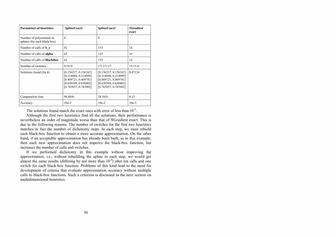
Thus, the model has several solutions that we want to find, rather than one. The following table illustrates performance of the implemented heuristics

compared to NGradient exact, which uses NGradient to look for the first solution.

29

Parameters of heuristics SplineExact1 SplineExact2 NGradientexact

Number of polynomials in splines (for each black box)

8 8 -

Number of calls of S_y 62 153 14

Number of calls of alpha 62 153 10

Number of calls of BlackBox 62 153 14

Number of switches 9+9+9 17+17+17 15+3+6

Solutions found (for k)

[0.156237, 0.156243] [0.314988, 0.314999] [0.469721, 0.469741] [0.630369, 0.630402] [0.783857, 0.783902]

[0.156237, 0.156243] [0.314988, 0.314999] [0.469721, 0.469741] [0.630369, 0.630402] [0.783857, 0.783902]

0.47124

Computation time 96.869s 38.365s 0.15

Accuracy 10e-2 10e-2 10e-5

The solutions found match the exact ones with error of less than 10-3. Although the first two heuristics find all the solutions, their performance is

nevertheless an order of magnitude worse than that of NGradient exact. This is due to the following reasons. The number of switches for the first two heuristics matches in fact the number of dichotomy steps. In each step, we must rebuild each black-box function to obtain a more accurate approximation. On the other hand, if an acceptable approximation has already been built, as in this example, then each new approximation does not improve the black-box function, but increases the number of calls and switches.

If we performed dichotomy in this example without improving the approximation, i.e., without rebuilding the spline in each step, we would get almost the same results (differing by not more than 10-4) after ten calls and one switch for each black-box function. Problems of this kind lead to the need for development of criteria that evaluate approximation accuracy without multiple calls to black-box functions. Such a criterion is discussed in the next section on multidimensional heuristics.

30

3.2 Multidimensional heuristics

To approximate black-box functions in the multidimensional case, interpolation by bilinear forms was used. In the two-dimensional case, spline interpolation or triangulation of the domain is possible, but hardly more promising.

Interpolation by bilinear forms

1. Construct a uniform grid in the domain of the arguments. 2. Call the black-box function at each grid point. 3. In each rectangular parallelepiped, construct a bilinear form from grid points and

function values (2n points), expressed in the general n-dimensional form with unknown coefficients. Solve the resulting linear system Ax = b with the Gauss method.

Solution algorithm

1. An initial domain for all variables of the black-box constraints is given (represented by an interval vector). The black-box functions in the model are approximated by bilinear forms and then the new model is computed.

2. If for each component of an interval vector we have epsxx ii <− , then this vector is declared to be a solution. Return to the previous saved state.

3. Subdivide each interval ],[ ii xx where (2) is false in two subintervals, save state and go to step 1 for the new interval vector.

Implementation and testing of the solution search algorithm in the multidimensional case faced the same problems as in the one-dimensional case due to multiple recalculations of the interpolating functions. Thus, it is necessary to evaluate the accuracy of the bilinear forms. Such a criterion may be based on the following algorithm. 1. Construct a grid with the given number of points and interpolate the black-

box constraint in each parallelepiped. 2. In each parallelepiped, choose one or several points, call the black-box

function and compare its value blackbox(xi) with the value of the interpolating bilinear form bilinear(xi) at this point: a. If |blackbox(xi) – bilinear(xi)| < eps, то then a new interpolation is

constructed (to use the new points as well), and the interpolation accuracy is assumed to be satisfactory.

b. If |blackbox(xi) – bilinear(xi)| > eps, then new nodes are added to each “unsatisfactory” parallelepiped, then continue with step 1 with interpolation in the new grid.

31

Test results

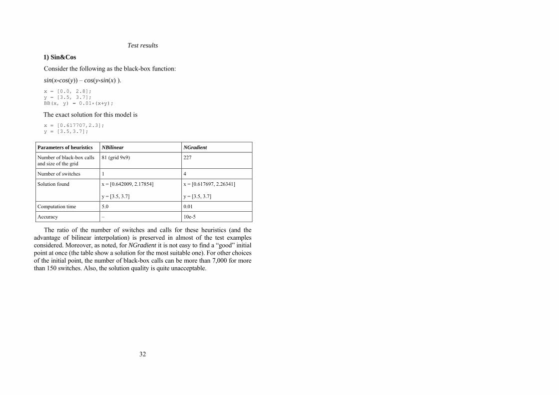
1) Sin&Cos

Consider the following as the black-box function:

sin(x*cos(y)) – cos(y*sin(x) ). x = [0.0, 2.8]; y = [3.5, 3.7]; BB(x, y) = 0.01*(x+y);

The exact solution for this model is x = [0.617707,2.3]; y = [3.5,3.7];

Parameters of heuristics NBilinear NGradient

Number of black-box calls and size of the grid

81 (grid 9x9) 227

Number of switches 1 4

Solution found

x = [0.642009, 2.17854]

y = [3.5, 3.7]

x = [0.617697, 2.26341]

y = [3.5, 3.7]

Computation time 5.0 0.01

Accuracy – 10e-5

The ratio of the number of switches and calls for these heuristics (and the advantage of bilinear interpolation) is preserved in almost of the test examples considered. Moreover, as noted, for NGradient it is not easy to find a “good” initial point at once (the table show a solution for the most suitable one). For other choices of the initial point, the number of black-box calls can be more than 7,000 for more than 150 switches. Also, the solution quality is quite unacceptable.

32

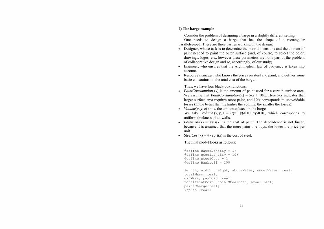
2) The barge example

Consider the problem of designing a barge in a slightly different setting. One needs to design a barge that has the shape of a rectangular

parallelepiped. There are three parties working on the design: • Designer, whose task is to determine the main dimensions and the amount of

paint needed to paint the outer surface (and, of course, to select the color, drawings, logos, etc., however these parameters are not a part of the problem of collaborative design and so, accordingly, of our study).

• Engineer, who ensures that the Archimedean law of buoyancy is taken into account.

• Resource manager, who knows the prices on steel and paint, and defines some basic constraints on the total cost of the barge.

Thus, we have four black-box functions: • PaintConsumption (x) is the amount of paint used for a certain surface area.

We assume that PaintConsumption(x) = 5*x + 10/x. Here 5*x indicates that larger surface area requires more paint, and 10/x corresponds to unavoidable losses (in the belief that the higher the volume, the smaller the losses).

• Volume(x, y, z) show the amount of steel in the barge. We take Volume (x, y, z) = 2z(x + y)*0.01+xy*0.01, which corresponds to uniform thickness of all walls.

• PaintCost(x) = sqr t(x) is the cost of paint. The dependence is not linear, because it is assumed that the more paint one buys, the lower the price per unit.

• SteelCost(x) = 4 * sqrt(x) is the cost of steel.

The final model looks as follows: @define waterDensity = 1; @define steelDensity = 10; @define steelCost = 1; @define Bankroll = 100; length, width, height, aboveWater, underWater: real; totalMass: real; ownMass, payLoad: real; totalPaintCost, totalSteelCost, area: real; paintCharge:real; inputs :real;

33

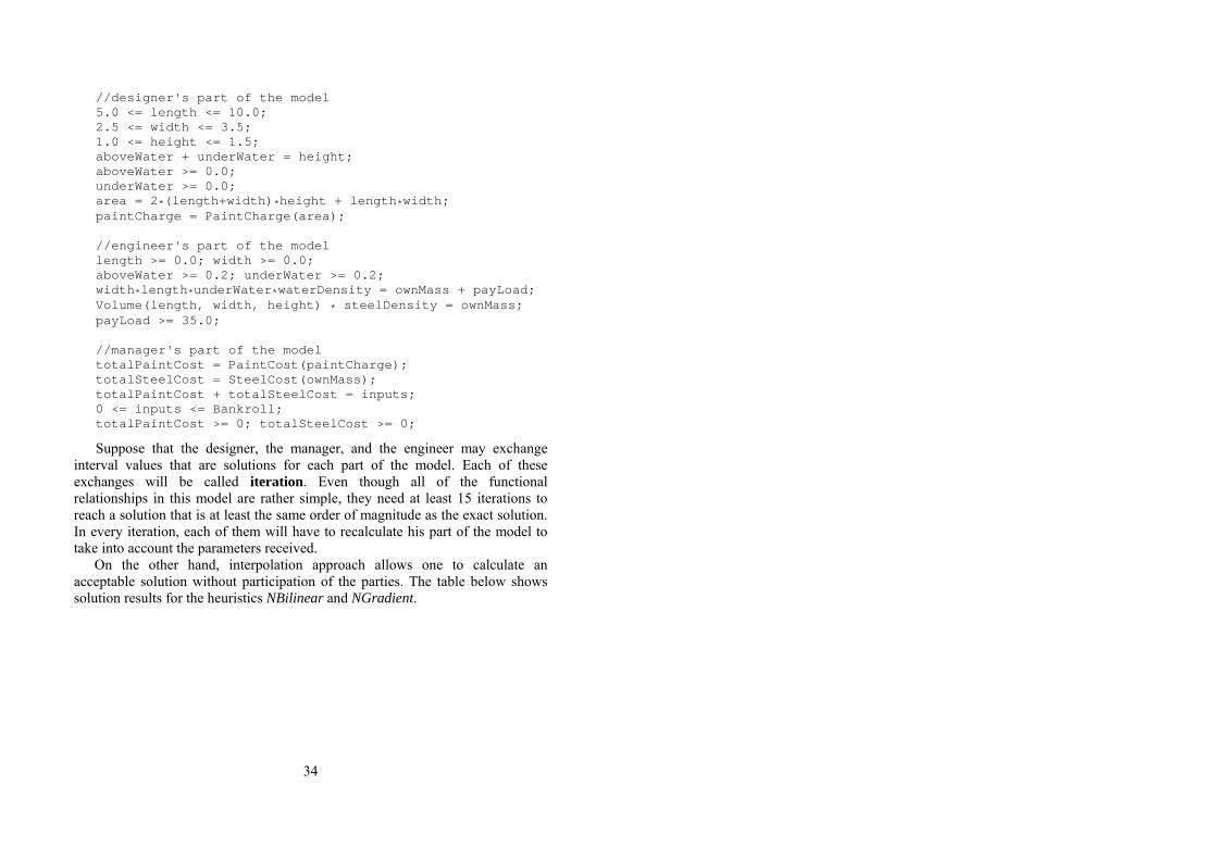
//designer's part of the model 5.0 <= length <= 10.0; 2.5 <= width <= 3.5; 1.0 <= height <= 1.5; aboveWater + underWater = height; aboveWater >= 0.0; underWater >= 0.0; area = 2*(length+width)*height + length*width; paintCharge = PaintCharge(area); //engineer's part of the model length >= 0.0; width >= 0.0; aboveWater >= 0.2; underWater >= 0.2; width*length*underWater*waterDensity = ownMass + payLoad; Volume(length, width, height) * steelDensity = ownMass; payLoad >= 35.0; //manager's part of the model totalPaintCost = PaintCost(paintCharge); totalSteelCost = SteelCost(ownMass); totalPaintCost + totalSteelCost = inputs; 0 <= inputs <= Bankroll; totalPaintCost >= 0; totalSteelCost >= 0;

Suppose that the designer, the manager, and the engineer may exchange interval values that are solutions for each part of the model. Each of these exchanges will be called iteration. Even though all of the functional relationships in this model are rather simple, they need at least 15 iterations to reach a solution that is at least the same order of magnitude as the exact solution. In every iteration, each of them will have to recalculate his part of the model to take into account the parameters received.

On the other hand, interpolation approach allows one to calculate an acceptable solution without participation of the parties. The table below shows solution results for the heuristics NBilinear and NGradient.

34

Parameters of heuristics NBilinear NGradient

Number of calls Volume (x,y,z) 64 (сетка 4x4x4) 77

Number of calls PaintCharge (x) 5 28

Number of calls PaintCost (x) 5 32

Number of calls SteelCost (x) 5 28

Number of switches 1+1+1+1 11+6+6+10

Solution found (for inputs) [27.6753, 30.4237] [27.6856, 30.4238]

Computation time 1.5 0.12

Accuracy – 10e-5

3.3 Findings

We can now summarize our study of applicability of the interpolation approach and the main results. • The use of interpolation algorithms for representation of black-box functions

by splines or bilinear forms is justified and in most cases satisfies the requirements.

• The solution search algorithms that improve interpolation quality in new steps are not usable in the current implementation.

• There is a need to develop criteria that evaluate accuracy of the interpolation constructed.

35

CONCLUSION

The collaborative design support system should significantly simplify implementation of tools for collaboration in a broad range of applications using constraints in problem statement. The combination of a flexible architecture and power methods of constraint processing, optimized for distributed operation, allow us to hope for successful implementation and subsequent dissemination of the system. The next step in the work on LCS should be a final clarification of the architecture and interfaces and beginning of implementation of the system. In the computation part, we need to focus on methods of solution search that are optimized for distributed computation and robust with respect to interpolation errors, on the one hand, and on the development of criteria for estimating interpolation accuracy, on the other hand. In addition, the base collection of models should certainly be expanded, both for comprehensive testing of the solutions and for demonstration of their capabilities.

36

REFERENCES

1. S. Preis, S. and Sidorov, V., Collaborative Design-1: Using Intervals, Constraints, and Interval Solver for Collaborative Design subsystem implementation, Preprint 6, LEDAS Ltd., Novosibirsk, 2003.

2. Shvetsov, I., Telerman, V. and Ushakov, D., NeMo+: Object-Oriented Environment for Subdefinite Computations, Proc. PPCP’97, Springer-Verlag, 1997 (LNCS 1330).

3. Ward, A. C., Liker, J. C., Sobek, D. C. and Cristiano, J. J., Set-based concurrent engineering and Toyota, ASME/DETC’94, Sacramento, California, Vol. DE 68, 1994. – pp. 79–90.

4. Sidorov, V. and Telerman, V., Using Black-Box Functions in Constraint Programming Environment, Proc. PSI’03, Novosibirsk, Russia, 2003.

5. Yannou, B., Simpson T. W. and Barton R. R., Towards a Conceptual Design Explorer Using Metamodeling Approaches and Constraint Programming, Proc. DETC’03, Chicago, Illinois, 2003.

6. Sidorov, V., Constraint programming with black boxes, Preprint №2, Ledas, Ltd., Novosibirsk, 2003 (in Russian).

37

38

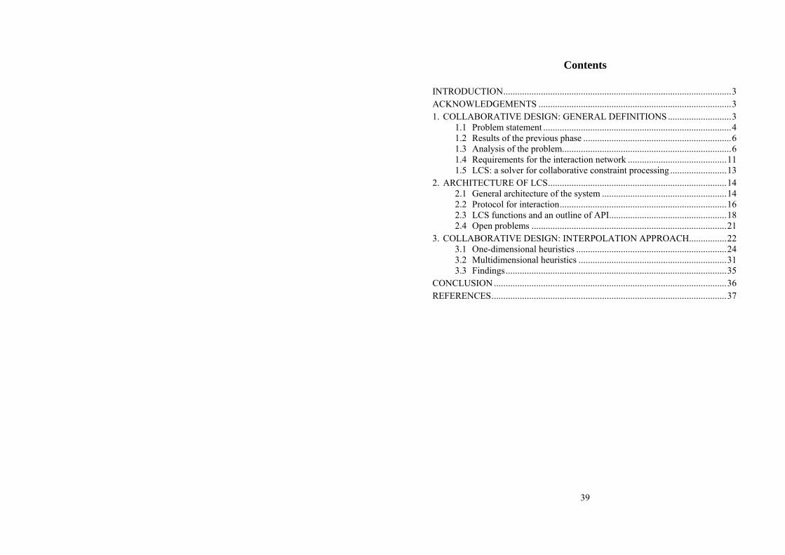
Contents

INTRODUCTION.................................................................................................3 ACKNOWLEDGEMENTS ..................................................................................3 1. COLLABORATIVE DESIGN: GENERAL DEFINITIONS...........................3

1.1 Problem statement ................................................................................4 1.2 Results of the previous phase ...............................................................6 1.3 Analysis of the problem........................................................................6 1.4 Requirements for the interaction network ..........................................11 1.5 LCS: a solver for collaborative constraint processing ........................13

2. ARCHITECTURE OF LCS............................................................................14 2.1 General architecture of the system .....................................................14 2.2 Protocol for interaction.......................................................................16 2.3 LCS functions and an outline of API..................................................18 2.4 Open problems ...................................................................................21

3. COLLABORATIVE DESIGN: INTERPOLATION APPROACH................22 3.1 One-dimensional heuristics ................................................................24 3.2 Multidimensional heuristics ...............................................................31 3.3 Findings..............................................................................................35

CONCLUSION ...................................................................................................36 REFERENCES....................................................................................................37

39

S. Preis, N. Snytnikov, D. Ushakov

COLLABORATIVE DESIGN-2 (LCS): CONCEPT, ARCHITECTURE, AND COMPUTATION METHODS

Preprint 8

Reviewed by V. Telerman Translated by A. Mullagaliev Edited by Е. Semoukhina Signed for publication 16.02.2004 50 copies printed