Supplementary Material 1

Life cycle assessment and costing of urine source separation:

Focus on nonsteroidal anti-inflammatory drug removal

Kelly A. Landry and Treavor H. Boyer

48 pages

12 tables

16 figures

S1

Table of ContentsS1. Determination of functional unit..........................................................................................5S2. Life cycle inventory...................................................................................................................7

S2.1. Flush water.........................................................................................................................7

S2.2. Centralized wastewater treatment......................................................................................8

S2.3. Ozonation of wastewater...................................................................................................10

S2.4. Urine source separation infrastructure............................................................................11

S2.5. Urine transport.................................................................................................................12

S2.6. Vacuum sewer system........................................................................................................13

S2.7. Ion-exchange treatment and disposal...............................................................................14

S2.8. Nutrient recovery..............................................................................................................18

S2.9. Estimation of pharmaceuticals in urine............................................................................19

S3. Materials and methods for bench scale ion-exchange column experiments.......................24S3.1. Synthetic human urine.......................................................................................................24

S3.2. Pharmaceuticals and estimated realistic concentrations.................................................24

S3.3. Ion-exchange resin............................................................................................................25

S3.4. Column tests......................................................................................................................25

S3.5. Sample preparation...........................................................................................................25

S3.6. Analytical methods............................................................................................................26

S4. Life cycle cost parameters.......................................................................................................27S5. Pharmaceutical characterization factors..................................................................................28S6. Uncertainty and sensitivity analysis input parameters and costs.............................................29S7. TRACI impact assessment results...........................................................................................31S8. Impact of resin regeneration and brine incineration................................................................40S9. Impact of urine collection by vacuum truck and vacuum sewer.............................................41S10. Non-carcinogenic human toxicity impact.............................................................................42References......................................................................................................................................43

S2

List of Tables

Table S1. Average urination volumes and frequency for asymptomatic men and women............5Table S2. Total number of weekdays during the fall, spring, and summer semesters, excluding major holidays; data from the University of Florida 2014–2015 academic calendar......................6Table S3. Estimated urine production for entire UF campus over different time periods..............6Table S4. Daily refuse route distance (km) traveled during fall, spring, and summer semesters.11Table S5. Mass of diclofenac (DCF), ibuprofen (IBP), ketoprofen (KTP), and naproxen (NPX) sorbed onto AER (mg) and desorbed from AER using a 5% NaCl, 50% methanol regeneration solution..........................................................................................................................................14Table S6. Inventory data for ion-exchange vessel components; data provided by Tonka Water (personal communication).............................................................................................................15Table S7. Inventory data for incineration of a regeneration brine at a cement kiln planta............17Table S8. Recommended defined daily dose (DDD), fraction of dose excreted in urine as the parent compound (Fex), and estimated pharmaceutical concentrations in urine............................23Table S9. Unit cost of inventory items.........................................................................................26Table S10. USEtox characterization factors (human toxicity in cases·kg–1 and ecotoxicity in PAF·m3·day·kg–1) for diclofenac, ibuprofen, ketoprofen, and naproxen....................................27Table S11. Baseline, minimum, and maximum values used for various input parameter assumptions....................................................................................................................................28Table S12. Baseline, minimum, and maximum values used for various cost assumptions..........29

S3

List of Figures

Figure S1. Bench scale column results for removal of diclofenac (DCF), ibuprofen (IBP), ketoprofen (KTP), and naproxen (NPX) by anion-exchange resin...............................................15Figure S2. Manufacturer data and resulting linear regressions of fiberglass tanks......................16Figure S3. Manufacturer data and resulting linear regressions of pump power ..........................17Figure S4. Relative frequency diagram of ibuprofen concentrations in urine..............................24Figure S5. Normalized TRACI impact score for centralized wastewater treatment, and urine source separation...........................................................................................................................32Figure S6. Comparison of ozone depletion impacts (kg CFC-11 eq.)..........................................33Figure S7. Comparison of global warming impacts (kg CO2 eq.)...............................................34Figure S8. Comparison of smog impacts (kg O3 eq.)..................................................................35Figure S9. Comparison of acidification impacts (kg SO2 eq.).....................................................36Figure S10. Comparison of eutrophication impacts (kg N eq.)....................................................37Figure S11. Comparison of carcinogenic impacts (CTUh)..........................................................38Figure S12. Comparison of respiratory effects impacts (kg PM2.5 eq.)......................................39Figure S13. Comparison of fossil fuel depletion impacts (MJ surplus).......................................40Figure S14. Impact assessment results for the regeneration process compared to incineration of the regeneration brine....................................................................................................................41Figure S15. Normalized TRACI impact score (PE) of vacuum truck collection compared to the vacuum sewer collection................................................................................................................42Figure S16. Comparison of non-carcinogenic human toxicity impact (CTUh)...........................43

S4

S1. Determination of functional unit

Urine production at the University of Florida (UF) was estimated from solid waste production

according to UF annual refuse routes (personal communication with UF Physical Plant

Department). The refuse routes included collection locations, collection days (e.g., Monday–

Thursday, Monday and Thursday only), and dumpster volumes. Some buildings shared

dumpsters, which are labeled according to the nearest building. If one building or cluster of

buildings (e.g., dormitories) had multiple dumpsters, they were consolidated into one

cumulative-volume dumpster. This reduced a total of 188 urine-producing buildings to 125

decentralized collection areas. UF student, faculty, and staff produce 1.46 lb waste/person∙d

(0.662 kg waste/person∙d) and 0.76 lb waste/person∙d (0.345 kg waste/person∙d) of that waste

is landfilled (Townsend et al., 2015). The approximate density of landfilled waste at UF is 75.4

lb/yd3 (44.7 kg/m3) (Townsend et al., 2015). It was assumed that at the time of collection, the

dumpsters were filled to capacity (personal communication with UF Physical Plant Division),

and non-collection days the dumpsters were assumed to be empty. Building-level waste

production and per capita waste production were used to estimate daily building occupancy (Eq.

S1).

Building occupancy=( Dumpster capacity , yd3 )(75.4 lby d3 )( person−day

0.76 lb ) Eq. S1

Daily urination events at the building-level were estimated based on urination frequency

and number of hours a building was assumed to be occupied (Eq. S2). According to a 7-day

sleep log of 237 people, college-aged students on average sleep 6.40 h per night resulting in 17.6

S5

Ex. Daily building occupancy for a building with a 6 yd3 dumpster filled to capacity

Building occupancy=(6 y d3

day )(75.4 lby d3 )( person−day

0.76 lb )=595 people

waking h/d It was assumed that residence halls were occupied for 9.14 h/d (Ishii and Boyer,

2015), and all other campus buildings were occupied for 8 h/d. Outlined in Table S1 are the

average urination volumes and frequency for asymptomatic men and women (FitzGerald et al.,

2002, Latini et al., 2004).

Urination events=(Building occupancy ) ( Hours o ccupied ,h )((0.4 voidsh ) (0.46 )+(0.45 voids

h ) (0.54 ))Urination events=(Building occupancy ) ( Hours occupied ,h )(0.428 voids

h ) Eq. S2

Table S1. Average urination volumes and frequency for asymptomatic men and women.Men Women

Volume, L d–1 1.65a 1.62b

Total daytime voids 7a 8b

Total nighttime voids 0a 0b

Mean voided volume, mL void–1 237a 204b

Average hours awake, h c 17.6 17.6Urination frequency, void h–1 d 0.40 0.45a Latini et al. (2004)b FitzGerald et al. (2002)c Tsai and Li (2004)d Calculated by dividing total daytime voids by average hours awake

Based on enrollment and employment data, UF population is composed of 46% males

and 54% females (UF, 2015, 2014b). The volume of urine produced daily was estimated using

equation S3.

Volumeurine produced , Lday

=(Urination events )( (0.46 )(0.237 Lvoid )+(0.54 )(0.204 L

void ))Volume urine produced , L

day=(Urination events )(0.219 L

void ) Eq. S3

S6

Ex. Daily urination events in a non-residence building occupied by 595 people

Urination events=(595 people )(8 hday )(0.427 voids

h )=2,032 urinationevents

Discrete values for urine production was estimated for each day of the week (Monday–

Sunday), therefore the annual urine production was estimated by multiplying daily urine

production by the number of days that campus was assumed to be occupied during the academic

year (Table S2). The 2014–2015 UF academic calendar was used to estimate the number of days

that students, faculty, and staff were present on campus (UF, 2014a). It was assumed campus

was closed over major holidays (e.g., Thanksgiving, Christmas, spring break, and breaks

between semesters), resulting in no urine production. Table S3 lists the estimated daily, 60-day,

and annual urine production for all of University of Florida campus.

Table S2. Total number of weekdays during the fall, spring, and summer semesters, excluding major holidays; data from the University of Florida 2014–2015 academic calendar.

Monday Tuesday Wednesday Thursday Friday Saturday SundayFall 17 17 15 16 15 15 15Spring 15 16 16 16 16 14 14Summer 12 12 12 12 12 11 10

Table S3. Estimated urine production for entire UF campus over different time periods.Time Urine production, m3

Dailya 39.760-dayb 2,381Annual 11,184a Average daily urine production over the weekb Average 60-day urine production

S2. Life cycle inventory

The following section describes the data sources and design parameters used to assess the

various treatment scenarios.

S2.1. Flush water

S7

Ex. Daily volume of urine produced in a non-residence building occupied by 595 people

Volume urine produced , Lday

=(2,032 urinationevents )(0.219 Lvoid )=445 L

day

Estimated potable flush water requirements were based on flush water specifications for

conventional toilets (6 L/flush), conventional urinals (3.8 L/flush), and urine diverting flush

toilets (0.05 L/small flush) and the estimated number of urination events over the course of a

year at UF (Ishii and Boyer, 2015, Zinckgraf et al., 2014). Operational phase inputs (e.g., energy,

chemicals, raw groundwater) for producing potable water were included within the life cycle

boundary (Ishii and Boyer, 2015). Operational costs for potable water and electricity were based

on local utility rates (Ishii and Boyer, 2015).

S2.2. Centralized wastewater treatment

At the WRF, 15% and 32% of wastewater effluent is reused as cooling water at a cogeneration

plant and landscape irrigation across campus, respectively (FDEP, 2015). The remaining 51% is

discharged by deep well injection. Deep well injection of municipal wastewater is conducted

primarily in Florida (EPA, 2012). In the United States, 14,651 out of 15,837 wastewater

treatment plants discharge to surface waters (Rice and Westerhoff, 2015). To make this study

transferable across communities in the U.S. and elsewhere, it was assumed that non-reclaimed

wastewater was discharged to surface water. Only the reclaimed water and surface discharge

effluent were considered within the system boundary of the LCA; water sent to the cogeneration

plant was assumed to have negligible impact on the environment with respect to

pharmaceuticals. Waste sludge collected during secondary clarification is transported off campus

to the city’s wastewater treatment plant for further processing and land application. The

environmental impact of biosolids was considered outside the scope of this study because the

treatment facility ceased land application of biosolids in February 2016 and currently disposes of

biosolids in a landfill (personal communication with J.H. Hope, June 26, 2016). Several

alternative disposal options are currently under review. The most cost effective recommended

S8

option is waste-to-energy disposal (GRU, 2011). Furthermore, the effect urine source separation

has on the composition of biosolids at centralized wastewater treatment is unknown. Jimenez et

al. (2015) modeled the effect of urine source separation on biological wastewater treatment but

not necessarily how the composition of biosolids would change, with respect to N and P content.

Due to the complexity of wastewater modeling, the N and P content of biosolids was considered

outside the scope of this model. N and P were assumed to be partially removed by biological

treatment (Ishii and Boyer, 2015).

The electricity and cost requirements for urine treatment at the centralized wastewater

treatment plant were based on the influent volumetric flow of urine and urine flush water and the

flow normalized electricity use at the plant. (Ishii and Boyer, 2015). Costs were based on local

utility rates (Ishii and Boyer, 2015). For scenarios AWWT and BWWT,O3, the impact of centralized

wastewater treatment pertained only to inputs related to the functional unit, i.e., the influent flow

was attributed to the total volume of urine (11,184 m3) and associated urine flush water from

conventional toilets and urinals, and did not account for additional wastewater inputs (e.g.,

greywater). Similarly, for scenarios C–F, the influent flow was attributed to the total volume of

urine and urine flush water from urine diverting flush toilets. At UF, one central department (i.e.,

Physical Plant Division (PPD)) maintains all operations on campus, including irrigation and

grounds maintenance (e.g., fertilization with commercial fertilizers). For all scenarios it was

assumed that 84.3% and 49.8% of influent N and P mass loads were removed during centralized

treatment with no nutrient recovery (Ishii and Boyer, 2015).

Pharmaceutical removal for each compound was estimated using the average pharmaceutical

removal by biological wastewater treatment in literature (Fernandez-Fontaina et al., 2012,

Hollender et al., 2009, Joss et al., 2005, Lindqvist et al., 2005, Margot et al., 2013, Rivera-Utrilla

S9

et al., 2013, Rosal et al., 2010, Salgado et al., 2012, Santos et al., 2007, Ternes, 1998). The N and

P that remain in the fraction of treated wastewater effluent discharged to surface water was

considered an emission. The N and P in the fraction of treated wastewater used as reclaimed

water in landscape irrigation was assumed to be completely taken up by turf grass. Reclaimed

water containing 9 mg/L N may be applied at a rate of 2 cm/week without N leaching

(Hochmuth et al., 2013). This corresponds to ~8900 kg N/year that may be applied to UF’s 235

acres of active irrigation on campus. It was estimated that 571 kg N and 558 kg N was applied to

landscape irrigated with reclaimed water in scenarios A–B and C–H, respectively. The mass of

pharmaceutical remaining in wastewater effluent was considered an emission to surface water or

an emission to non-industrial, urban land for the respective fractions discharged to surface water

or used as landscape irrigation.

S2.3. Ozonation of wastewater

For scenario BWWT,O3, an additional ozonation step was added to the centralized wastewater

treatment plant in scenario AWWT to treat the influent urine and urine flush water. Pharmaceutical

destruction for each compound was estimated using the average pharmaceutical destruction by

ozonation of secondary wastewater in literature (Hollender et al., 2009, Huber et al., 2003,

Margot et al., 2013, Rosal et al., 2010, Ternes, 1998). The system boundary included the

infrastructure requirements for the ozone contactor, production of oxygen, electricity, transport,

and cooling water for ozone production. The material inputs for infrastructure did not include the

ozone generator, due to a lack of data. The ozone contactor was sized to treat the entire influent

flow at the wastewater treatment plant (i.e., urine, flush water, feces, and greywater). The ozone

contactor was assumed to have an HRT of 5 min and was designed to meet specifications

outlined by Snyder et al. (2014). The ozone contactor was assumed to have 4 cells (1.2 m/cell),

S10

5.8 m of submergence, and 1.5 m of freeboard. The length and width of the contactor were 5 m

and 0.64 m, respectively (personal communication with Mike Witwer, 2016). Material inputs for

the ozone contactor only included concrete requirements. The infrastructure costs included the

total ozonation system (e.g., ozone contactor, ozone generator, installation costs, yard piping,

landscaping, electrical and construction, and labor) (Snyder et al., 2014). Inventory data for the

operational phase (e.g., electricity, oxygen, water, and transport) were estimated on the basis of

treating 1 m3 of wastewater at a full-scale plant according to Muñoz et al. (2009).

S2.4. Urine source separation infrastructure

There are 5,666 toilets and 1,237 urinals in 189 buildings on UF campus whose wastewater is

conveyed to the UF WRF. For scenarios C–H it was assumed that the conventional toilets and

urinals were replaced with urine diverting toilets and waterless urinals. Conventional fixtures

were replaced to make a fair economic comparison with other scenarios that use waterless urinals

and urine-diverting flush toilets. Costs for replacing toilets and urinals (conventional and

alternative fixtures) were based on market prices (Ishii and Boyer, 2015, Kohler, 2016, U.S.

EPA, 2016). It was assumed that the urine diverting toilets had an 80% separation efficiency

(Vinnerås, 2001), and that these were used exclusively by women. Waterless urinals were

assumed to have 100% separation efficiency. The manufacturing and installation of conventional

(scenarios AWWT and BWWT,O3) and urine diverting fixtures (scenarios C–H) were assumed to be

equal, thus negating these fixtures in the environmental assessment. Material and formation

processes and associated costs required for pipes and storage tanks were included in this

assessment with an expected pipe lifetime of 50 years (Ishii and Boyer, 2015). A separate urine

collection piping system was added to divert urine and urine flush water (generated by urine-

diverting flush toilets only) from the general waste stream and collected in decentralized HDPE

S11

storage tanks located at 125 collections areas on campus. Pipe requirements for urine diverting

toilets were based on the requirements for a model apartment in Remy (2010) and the

requirements for urinals were assumed to be equivalent.

Urine was assumed to be stored for 60 days to inactivate potential pathogens and/or fecal

contamination (Nordin et al., 2009, Vinnerås et al., 2008). Decentralized HDPE urine storage

tanks were sized according to the estimated volume of urine produced at each of the

decentralized treatment areas on campus. For scenarios Ctruck,landfill and Dtruck,regen, one HDPE tank

was located at each decentralized collection area and sized to hold the estimated daily maximum

volume of urine produced before being collected and transported to a central location for

treatment on campus. The material and formation inputs for the HDPE urine storage tanks per

functional unit was estimated using previous research and an expected tank lifetime of 40 years

(Ishii and Boyer, 2015). Decentralized HDPE storage tanks were estimated using a linear

regression for tank costs as a function of storage volume (Ishii and Boyer, 2015). The centralized

treatment area was equipped with two bolted steel and polyurethane lined storage tanks, where

one tank collects new urine and urine flush water while the other stores previously collected

urine and urine flush water for stabilization and disinfection. The steel tanks were assumed to

meet AWWA D-103 steel tank specifications and lined with polyurethane to protect the steel

from corrosion (AWWA, 2009, Richardson, 1999, STI/SPFA, 2016). Centralized urine storage

tank costs were estimated using a cost analysis tool for AWWA D-103 steel water storage tanks

(STI/SPFA, 2016). For scenarios Gdecen,landfill and Hdecen,regen, urine was collected, stored, and treated

at the building level. In these scenarios, each collection area required two HDPE tanks for

simultaneous collection and storage disinfection of urine and urine flush water.

S2.5. Urine transport

S12

For scenarios Ctruck,landfill and Dtruck,regen, urine was collected following the same refuse routes

established by UF for municipal solid waste. In SimaPro, transportation (kgkm) is quantified by

the emissions and diesel fuel consumption for a truck that has an efficiency of 1.72×104 kgkm/L

diesel (PRé Consultants, 2014). UF refuse routes are subdivided into north, central, and south

campus routes. The roundtrip distance for each route was estimated by plotting the dumpster

locations (i.e., decentralized collection areas) on Google Earth and using the “path” function to

best guess the route and estimated distance traveled for every day of the week, as shown in Table

S4.

Table S4. Daily refuse route distance (km) traveled during fall, spring, and summer semesters.Fall & Spring Monday Tuesday Wednesday Thursday Friday Saturday SundayNorth Campus 12 12 12 12 12 10 0Central Campus 14 16 14 10 16 8 0South Campus 14 18 15 20 13 10 0SummerNorth Campus 12 8 12 9 12 10 0Central Campus 13 12 14 10 14 8 0South Campus 11 15 14 20 11 10 0

For ease of calculation, decentralized areas within each route (i.e., north, central, and

south campus) were assumed to be equidistant. For example, the north route is approximately 12

km and the 27 decentralized areas within that route were assumed to be 0.43 km apart. To

account for the incremental increase in weight with the addition of urine in the vacuum truck at

each pickup location, the daily urine transport for the north (tn), central (tc), and south (ts) campus

routes was estimated using equation S4,

t n ,c , s=∑i=1

n

d i mi+d i+1 ( mi+mi+1)+…+dn(mi+…+mn) Eq. S4

where dn is the incremental distance between each decentralized location (km) and mn is the mass

of urine (kg) collected at each location. Discrete values for urine transport was estimated at each

decentralized area for every day of the week (Monday–Sunday). The maximum capacity of the

S13

vacuum truck was assumed to be 4,000 gal (15,142 L). If the cumulative daily volume at each

route exceeded the maximum capacity, it was assumed the truck stopped collecting urine and

returned to the centralized location to unload the urine before completing the route. Annual

transport was estimated by multiplying daily transport by the number of days that urine was

assumed to be collected during the academic year (Table S2). The cost of urine transport was

estimated based on market price of diesel fuel (USEIA, 2015).

S2.6. Vacuum sewer system

For scenarios Esewer,landfill and Fsewer,regen, a vacuum sewer system was assumed to be installed to

convey source separated urine and urine flush water to a centralized location on campus for

further treatment. The wastewater planning model for decentralized systems (version 1.0)

(Buchanan et al., n.d.) was used to estimate cost, 4” (102 mm) PVC pipe requirements, energy

for the vacuum and wastewater transfer pumps, and pump station to implement a vacuum sewer

system servicing 188 buildings on UF campus. It was assumed that 100% of the collection

system was vacuum based and 152.4 m was the typical distance between each source. The

vacuum sewer system was assumed to have a lifetime of 60 years. In SimaPro, a gravity pump

station inventory item was substituted for the vacuum pump station.

S2.7. Ion-exchange treatment and disposal

Bench-scale column experiments were used to estimate full-scale column design for

pharmaceutical removal. A complete description of experimental materials and methods is

provided in a separate section in section S3. Full-scale columns were designed to achieve

maximum DCF removal, which was the pharmaceutical most selective for the resin. The

operating capacity was calculated as the mass of DCF sorbed onto the resin before removal of

DCF fell below the maximum achievable level (i.e., mass of DCF sorbed onto the resin when

S14

DCF removal <98% after 1266 BV of treatment). The results of the treatment and regeneration

experiments are shown in Figure S1 and Table S5, respectively.

Figure S1. Bench scale column results for removal of diclofenac (DCF), ibuprofen (IBP), ketoprofen (KTP), and naproxen (NPX) by anion-exchange resin.

Table S5. Mass of diclofenac (DCF), ibuprofen (IBP), ketoprofen (KTP), and naproxen (NPX) sorbed onto AER (mg) and desorbed from AER using a 5% NaCl, 50% methanol regeneration solution.

Pharmaceutical Mass sorbed (mg) Mass desorbed (mg) % RegenerationDCF 25.6 3.63 14%IBP 2.4 0.331 14%KTP 18.7 0.15 1%NPX 4.6 1.346 30%

Columns were scaled to treat the entire volume of urine and urine flush water collected

by the source separation system, with one preconditioning cycle at the beginning (scenarios C–

H) and one regeneration cycle (scenarios Dtruck,regen, Fsewer,regen, and Hdecen,regen) at the end of the year.

Energy, water, and chemical requirements were included for 10 BV of resin preconditioning

using 5% NaCl and 10 BV of regeneration solution using 5% NaCl and 50% methanol. The

column was designed to maintain an EBCT of 8.3 min and minimum HLR of 10 m/h (Taute et

al., 2013). For scenarios C–F, one large column was used to treat the entire volume of urine, and

for scenarios Gdecen,landfill and Hdecen,regen, one column was scaled to treat urine produced annually at

S15

each decentralized location. Market values for fiberglass ion-exchange vessels of varying sizes

were used to generate a linear regression for vessel cost as a function of volume (Fresh Water

Systems, 2016, Water Softeners & Filters, 2016). The material input and cost of the fiberglass

column vessel were estimated using linear regressions shown in Figure S2 (Choe et al., 2013).

Figure S2. Manufacturer data and resulting linear regressions of fiberglass water softener tank (a) empty weight (kg) as a function of volume (m3) and (b) cost ($) as a function of volume (m3); data provided by waterpurification.pentair.com, reskem.com, freshwater.

Additional components (e.g., valves, pressure indicator, etc.) were estimated from a pilot

scale ion-exchange vessel (personal communication with a representative at Tonka Water). A

description of the components included in each ion-exchange column and list of materials and

respective masses are provided in the SI (Table S6). Pump power requirements (kW) was

estimated as a function of flow rate using a linear regression (Figure S3) developed from various

centrifugal pump specifications.

S16

Table S6. Inventory data for ion-exchange vessel components; data provided by Tonka Water (personal communication).Component Material Mass, kgd

Ball valves with lever Brass 1.34Air release valve PVC 0.195Pressure indicatorsa Steel 0.029

Aluminum 0.029Bronze 0.029Brass 0.029

1” Tee connectors to tank HDPE 3.63×10–3

1” ID × 1/4” OD Tubingb PVDF 0.61/4” ID × 3/8” ODc Tubingc PVDF 0.490a Pressure indicator composed of multiple materials, total mass of pressure indicator equally distributed among componentsb Tubing used for ion-exchange vessel in scenarios C–F onlyc Tubing used for ion-exchange vessels in scenarios G and H onlyd Non-normalized mass of components; mass of ion-exchange vessel and components normalized by 40 year lifetime in LCA inventory

Figure S3. Manufacturer data and resulting linear regressions of centrifugal pump power specifications; data provided by grainger.com and northerntool.com.

Disposal of the spent resin or regeneration brine was included within the system

boundary because they were considered integral to the overall life cycle impacts of the treatment

process. For scenarios Gdecen,landfill and Hdecen,regen, the fiberglass ion-exchange columns at each

decentralized location were collected and transported to a central location for further processing.

For scenarios Ctruck,landfill, Esewer,landfill, and Gdecen,landfill, spent resin was transported and disposed of in

a local Class I landfill. Disposal of the resin was modeled as polystyrene because it constitutes

the backbone of the ion-exchange resin (Choe et al., 2013). In scenarios Dtruck,regen, Fsewer,regen, and

S17

Hdecen,regen, the regeneration brine was transported to a local cement kiln plant where it was

incinerated. The use of waste solvents as fuel in cement production reduces the need for fossil

fuels. Ecosolvent 1.0.1 life cycle assessment tool was used to generate the life cycle inventory

data for solvent combustion as a function of the elemental solvent composition (e.g., 5% NaCl

and 50% methanol) and technology used (e.g., incineration at a cement kiln) (Weber et al.,

2006). The resulting inventory included the amount of fossil fuels substituted by waste solvents

and changes in the atmospheric emissions (Table S7); changes to infrastructure at the cement

kiln plant were not considered. The Ecosolvent model for solvent incineration in a cement kiln

was based on average technology used in Switzerland (Seyler et al., 2005). The cost of chemicals

(i.e., methanol and NaCl) and potable water used during the preconditioning and regeneration

process were based on market price (Ishii and Boyer, 2015, methanex, 2015, USGS, 2015).

Table S7. Inventory data for incineration of a regeneration brine at a cement kiln plant.a

kg per m3 of total regeneration solution volume (e.g., water + methanol)

Regeneration solution5% NaCl, 50% Methanol

Hard coal –148b

Heavy fuel oil –54.5Carbon dioxide –76.3Carbon dioxide fuel –621Nitrogen oxides –1.67Nickel –1.11×10–7

Copper –6.59×10–7

Zinc –1.10×10–4

Metals unspecified –1.43×10–5

Arsenic –3.09×10–7

Cadmium –4.45×10–5

Chromium –9.39×10–7

Mercury –8.86×10–5

Lead –1.01×10–4

a Inventory data obtained from Ecosolvent 1.0.0 software (Weber et al., 2006)b Negative values indicate an avoided impact (i.e., offset)

S2.8. Nutrient recovery

For scenarios C–H, struvite (MgNH4PO4∙6H2O) precipitation of urine, after ion-exchange

treatment, was conducted to recover maximum P in urine. It was assumed that all magnesium

S18

and calcium in collected urine was lost in the collection system due to spontaneous precipitation

of struvite and hydroxyapatite resulting in some nutrient loss (Udert et al., 2003). Magnesium

oxide (MgO) was dosed to stored urine to achieve a molar Mg:P ratio of 1.2:1 to achieve

maximum P recovery as struvite. The cost of magnesium oxide was based on market price (Ishii

and Boyer, 2015). The value of struvite fertilizer was estimated using a regression model of

common fertilizers and costs of contributing nutrients (Ishii and Boyer, 2015). In scenarios

Gdecen,landfill and Hdecen,regen, struvite precipitation was conducted every 60 days after storage

disinfection, collected and centrally stored in a HDPE tank. The recovered struvite can be used

directly as a slow-release fertilizer in place of conventional fertilizers (Johnston and Richards,

2003), and thus contributes to the environmental and cost benefits for scenarios C–H. For these

scenarios, conventional fertilizers were considered an “avoided product” in SimaPro, represented

as “monoammonium phosphate, as P2O5 at regional storehouse/RER U” and “monoammonium

phosphate, as N, at regional storehouse/RER U” (NH4H2PO4) because it is a commonly used

fertilizer product containing both N and P. It was assumed that the quality and size of

precipitated struvite was comparable to commercial granular fertilizers and that identical

commercial spreading machines were used for struvite or commercial fertilizers (Forrest et al.,

2008). This assumption negates the power requirements for spreading struvite or

monoammonium phosphate. Furthermore, emissions (e.g., ammonia, nitrous oxide, and

phosphorus) for commercial fertilizers and struvite fertilizers were assumed to be equivalent.

Ammonia emissions for multi-nutrient fertilizers (e.g., struvite, and monoammonium phosphate)

are quantified by an identical emission factor of 4% (Nemecek and Kägi, 2007). Furthermore,

nitrous oxide and phosphorus emissions are quantified as a function of N and P content in the

fertilizer (Nemecek and Kägi, 2007). Those emissions were also negated because struvite

S19

fertilizer is assumed to offset the equivalent amount of N and P in monoammonium phosphate.

One of the benefits of struvite precipitation from urine is the low heavy metal content compared

to commercial fertilizers. However, studies have shown that heavy metals in urine (e.g.,)

cadmium may be incorporated into the final struvite product, although to a much lesser extent

than what is found in commercial fertilizers (Lugon-Moulin et al., 2006, Ronteltap et al., 2007).

Therefore, cadmium emissions from struvite and monoammonium phosphate was included

within the LCA boundary. Cadmium content of struvite and monoammonium phosphate was

assumed to be 0.397 mg Cd/kg P2O5 and 97.5 mg Cd/kg P2O5, respectively (Lugon-Moulin et al.,

2006, Ronteltap et al., 2007).

S2.9. Estimation of pharmaceuticals in urine

Pharmaceutical concentrations in urine can vary as a function of fraction of population use,

duration of use, and rate of urine collection. A system of equations was used to estimate

pharmaceutical concentrations in urine as a function of these variables. All calculations were

based on urinary excretion rates of the pharmaceutical active ingredient in urine, pharmaceutical

metabolites were not considered in this study. Sample calculations are provided using ibuprofen

as the example pharmaceutical. According to Khan and Nicell (2010) the pharmaceutical

concentration in urine can be estimated as a function of the percentage of the population that is

using a particular pharmaceutical and the maximum pharmaceutical concentration that may be

present if 100% of the population consumed pharmaceuticals, as shown in Eq. S5 (Khan and

Nicell, 2010).

F c=C

C100Eq. S5

Where Fc is the fraction of the population that is currently using a pharmaceutical, C is the

pharmaceutical concentration in urine and C100 is the pharmaceutical concentration in urine if

S20

100% of the population consumed a pharmaceutical. This equation can be rearranged so that the

concentration in urine can be determined by Eq. S6:

C=F c ×C100 Eq. S6

C100 may be estimated by Eq. S7:

C100=DDD × Fex

UEq. S7

Where DDD (mg) is the defined daily dose of a pharmaceutical (Table S8). In this example, the

defined daily dose was based on the World Health Organization recommendation (Table S8)

(Holloway and Green, 2003), Fex is the fraction of the consumed dose excreted in urine as the

pharmaceutical active ingredient based on pharmacokinetics in literature (Table S8), and U is the

average urine excretion volume per person per day which is estimated to be 1.5 L/p/d (FitzGerald

et al., 2002, Latini et al., 2004).

The pharmaceutical concentration can be diluted by two additional factors: duration of

pharmaceutical use and urine storage collection time. Duration of pharmaceutical use is

expressed as a fraction of the urine storage collection time. For example, if the urine storage

collection time was one week and the maximum daily dose of a pharmaceutical was consumed

S21

Ex. What is the expected concentration of ibuprofen in urine?

The DDD of ibuprofen is 1,200 mg and the 7% of the ingested dose is excreted in urine as the parent compound (Lienert et al., 2007).

C100=(1,200 mg× 0.07 )

1.5 ( L/ p /d )=56 mg

L

Now the pharmaceutical concentration in urine as a function of population use can be estimated by the equation

C=F c ×56 mgL

This equation means that if 1% (Fc = 0.01) of the population was taking ibuprofen, the ibuprofen concentration in urine would be 560 μg/L. If 100% (Fc = 1) of the population were taking ibuprofen the concentration would be 56 mg/L which is equivalent to the amount excreted in urine for one person because it is not diluted by ibuprofen-free urine.

for one week, then the pharmaceutical was consumed for 100% of the collection time.

Conversely, if the pharmaceutical was consumed 1 day out of the 7-day collection time, the

pharmaceutical was consumed for 14.3% of the collection time. The percent duration of use can

be determined by Eq. S8:

Fd=du

dcEq. S8

Where Fd is the fraction of duration of use compared to collection time, du is the number of days

a pharmaceutical was consumed, and dc is the storage collection time in days. The total

concentration in urine over the entire collection period may be calculated by Eq. S9:

CT=C × Fd=C100 × F c × Fd Eq. S9

Where CT is the total pharmaceutical concentration in collected urine.

S22

One final variable that could impact pharmaceutical concentrations in urine is if different

fractions of the population consume pharmaceuticals for varying durations of time. For example,

if 25% of the population consumed a pharmaceutical for 10% of the collection time and then

15% of the population consumed the same pharmaceutical for 25% of the collection time. The

concentration of pharmaceuticals in urine is simply the summation of the total pharmaceutical

concentration in urine according to each pharmaceutical consumption scenario, as outlined in Eq.

S10:

CTn=CT1+CT2

+…C T n=C100∑i=1

n

FcnFdn

Eq. S10

S23

Ex. What is the concentration of ibuprofen in urine if 100 out of 100 students in a dorm consumed ibuprofen for 7 days and the urine collection time was 7 days? What if 25% of the students consumed ibuprofen for 4 days?

Fu=100100

=1

C=56 mgL

×1=56 mgL

Fd=77=1

CT=56 mgL

×1=56 mgL

Intuitively, this value makes sense because if the entire population of students consumes ibuprofen for the entire collection period, the pharmaceutical concentration would not be diluted and would simply equal C100.

Ex. What if 25% of the students consumed ibuprofen for 4 days?

Fu=0.25

C=56 mgL

×0.25=14 mgL

Fd=47=0.57

CT=14 mgL

× 0.57=7.98 mgL

Figure S4 is a frequency diagram of all the possible ibuprofen concentrations in urine for a

community for Fc and Fd range from 1% to 100%. The relative frequency is skewed to the right,

resulting in a non-normal distribution. For a non-normal distribution, the central tendency is best

measured by the median value in the dataset (Ott and Longnecker, 2004), or 10.7 mg/L

ibuprofen. For this model, it was assumed that DCF, IBP, KTP, and NPX were present in urine at

concentrations of 767, 10,735, 4,792, and 831 μg/L, respectively (Table S8). A lognormal

distribution was assumed for the data with a standard deviation of 1.31. The minimum and

maximum concentrations in urine were based on the 95% confidence interval of the lognormal

S24

Ex. What is the ibuprofen concentration in urine if 25 of 100 students in the dorm population consumed the pharmaceutical for 2 out of 7 days of collection time and a few days later 15 students consumed ibuprofen for 4 out of 7 days of the collection time?

CT=(56 mgL

× 25100

× 27 )+(56 mg

L× 15

100× 4

7 )=4 mgL

+4.8 mgL

CT=8.8 mgL

This value can be confirmed by individually calculating the mass pharmaceutical load (Mpharm) for each population fraction and determining the concentration of pharmaceuticals for the entire storage collection period.

M phar m1=(25 people ) (2days )(1.5 L

p ∙ d )(56 mgL )=4,200mg

M phar m2=(15 people ) (4 days )(1.5 L

p ∙ d )(56 mgL )=5,040 mg

Total pharmaceutical mass load:

M T=4,200 mg+5,040 mg=9,240 mg

Total urine production over 7 days:

(100 students )(1.5 Lp ∙d ) (7days )=1,050 L

Total pharmaceutical concentration in urine:

CT=9,240 m g1,050 L

=8.8 mgL

distribution and is defined by dividing or multiplying the median pharmaceutical concentration

in urine with the squared standard deviation (i.e., 1.71).

Figure S4. Relative frequency diagram of ibuprofen concentrations in urine for a community where 1–100% of the population is consuming ibuprofen (Fc) for 1–100% of the collection time (Fd).

Table S8. Recommended defined daily dose (DDD), fraction of dose excreted in urine as the parent compound (Fex), and estimated pharmaceutical concentrations in urine.Pharmaceutical DDD, mg Fex Median (minimum, maximum), μg/LDiclofenac (DCF) 100a 0.06b 767 (450, 1,308)Ibuprofen (IBP) 1,200a 0.07c 10,735 (6,294, 18,309)Ketoprofen (KTP)

300a 0.06d 1,230 (721, 2,098)

Naproxen (NPX) 500a 0.013e 831 (487, 1,417)a WHOCC (2013)b Sawchuk et al. (1995)c Lienert et al. (2007)d Houghton et al. (1984)e Sugawara et al. (1978)

S3. Materials and methods for bench scale ion-exchange column experiments

S3.1. Synthetic human urine

S25

Synthetic ureolyzed human urine was used for all experiments. The urine composition was based

on previous work (Landry et al., 2015), with adjustment to include the six endogenous

metabolites present at the greatest concentrations in urine (Bouatra et al., 2013).

S3.2. Pharmaceuticals and estimated realistic concentrations

Four pharmaceuticals were investigated for this study; the chemical characteristics were

described previously (Landry et al., 2015). Diclofenac sodium (CAS 15307-79-6, MP

Biomedicals), ibuprofen (CAS 311-21-95-4, Fluka Analytical), naproxen (CAS 26159-54-2,

Sigma-Aldrich), and ketoprofen (CAS 22071-15-4, Sigma-Aldrich) are all acidic

pharmaceuticals from the non-steroidal anti-inflammatory drugs (NSAIDs) pharmaceutical class.

A stock solution containing 1,000 mg/L of each solution was made by diluting the

pharmaceutical salts in methanol.

S3.3. Ion-exchange resin

A strong-base, polymeric anion exchange resins (AER), Dowex 22, was used in all experiments.

Dowex 22 is a strong-base, macroporous polystyrene AER functionalized with dimethyl ethanol

functional groups with a manufacturer’s total capacity of 1.2 meq mL–1. The AER was pre-

conditioned using NaCl, following a method described elsewhere (Landry and Boyer, 2013).

S3.4. Column tests

Fixed bed column runs were conducted in a glass column (0.7854 cm diameter) packed with 6

mL of Dowex 22 AER to obtain a height: diameter of at least 2:1 (Edzwald, 2011). All column

runs were performed under the same conditions by maintaining an empty bed contact time

(EBCT) and flow rate of 8.3 min and 0.72 mL/min, respectively. Synthetic ureolyzed urine was

spiked with the pharmaceutical stock solution at an initial concentration of 1,000 µg/L. 100 mL

of sample was collected every 12 h using an IS-95 interval sampler (Spectra/Chrom). Control

S26

samples were collected at the beginning and end of the column experiment. At the end of the run,

the column was regenerated using 10 BV of regeneration solution containing 5% NaCl, 50%

methanol by maintaining an EBCT and flow rate of 16.7 min and 0.36 mL/min, respectively.

S3.5. Sample preparation

Pharmaceutical samples from the column experiments were separated from the urine matrix

using a solid phase extraction (SPE) vacuum station (Supelco Visiprep) and phenyl SPE columns

(SiliaPrep, SiliCycle), evaporated, and reconstituted following a previously described method

(Magiera et al., 2014). The dry residue was dissolved in 1 mL of mobile phase (acetonitrile:25

mM KH2PO4 (pH 3) (40:60; v/v)) and 100 µL was injected into the HPLC-UV system (Hewlett

Packard 1050 series detector and Agilent 1100 series auto sampler).

S3.6. Analytical methods

Pharmaceutical concentrations for the batch regeneration experiments were measured using UV

absorbance (Hitachi U-2900) following a method described elsewhere (Landry and Boyer,

2013). Pharmaceutical concentrations for the column experiments were measured using HPLC-

UV (Hewlett Packard 1050 series detector and Agilent 1100 series auto sampler) at 230 nm,

equipped with a reversed-phase column (2.1 × 150 mm, 3 μm Ascentis RP-amide column;

Supelco, Bellefonte, PA). The mobile phase consisted of (A) a mixture of acetonitrile and 25

mM KH2PO4 (pH 3) (40:60 v/v), and (B) HPLC grade acetonitrile. Elution was performed by

increasing mobile phase B from 0% (5 min) to 50% (20 min), hold for 1 min, and decrease to 0%

(21.5 min) to re-equilibrate the baseline for 9.5 min. A seven-point calibration curve (0, 10, 50,

100, 500, 1,000, 5,000 µg L–1) was created by serial dilution of the stock standards previously

mentioned in mobile phase A. The minimum limit of detection (LOD) was 50 μg/L for DCF and

IBP, 10 μg/L for KTP and NPX. Pharmaceutical concentrations were set to the LOD if the

S27

effluent concentration fell below the LOD. One DCF sample in the treatment cycle fell below the

LOD. Eight KTP samples, two NPX samples, seven IBP samples, and two DCF samples fell

below the LOD in the regeneration cycle.

S28

S4. Life cycle cost parameters

Table S9. Unit cost of inventory items.

Input Unit Unit pricef Year of original cost data Justification

Impacted Scenarios

InfrastructureOzone system (30 years)a $ unit–1 $2,808,853 2011 Cost regression curve, as a function of plant capacity BConventional toilet (25 years)b $ fixture–1 $203 2015 Ishii and Boyer (2015) A, BConventional urinal (25 yearsb $ fixture–1 $355 2015 U.S. market price, www.us.kohler.com A, BUrine diverting flush toilet (25 years)b $ fixture–1 $700 2016 Ishii and Boyer (2015) C–HWaterless urinal (25 years)b $ fixture–1 $740 2016 U.S. market price, www.us.kohler.com C–HUrine piping (50 years)b $ fixture–1 $25 2015 Ishii and Boyer (2015) C–HSteel and HDPE lined urine central storage tanks (40 years)c

$ m–3

$272 2008 Cost estimation tool (STI/SPFA, 2016) C–F

HDPE storage tanks (40 years)b $ m–3

$29 2015 Linear regression of vessel cost as a function of volume (Ishii and Boyer, 2015)

C–H

Fiberglass ion-exchange vessel (10 years)d

$ m–3

$1,955 2015 Linear regression of vessel cost as a function of volume (Figure S2)

C–H

4” PVC vacuum sewer pipe (60 years)e $ m–1 $10 2009 Wastewater planning model (Buchanan et al., n.d.) E, FVacuum sewer station (60 years)e $ unit–1 $503,928 2009 Wastewater planning model (Buchanan et al., n.d.) E, FOperationPotable water $ m–3 $0.92 2015 Local utility rates (Ishii and Boyer, 2015) A–HLiquid oxygen $ kg–1 $0.12 2012 U.S. market price (Carollo Engineers, 2012) BVacuum sewer annual maintenance $ yr–1 $29,677 2009 Wastewater planning model (Buchanan et al., n.d.) E, FAnion exchange resin $ L–1 $12 2016 U.S. market price, www.apswater.com C–HElectricity $ kWh–1 $0.10 2015 Local utility rates (Ishii and Boyer, 2015) A–HSodium chloride $ kg–1 $0.20 2014 U.S. market price (USGS, 2015) C–HMethanol $ m3 $322 2015 U.S. market price, www.methanex.com D, F, HDiesel fuel $ L–1 $0.73 2015 U.S. market price, (USEIA, 2015) A–HMagnesium oxide $ kg–1 $0.21 2015 Ishii and Boyer (2015) C–HStruvite profit $ kg–1 $0.57 2013 Ishii and Boyer (2015) C–Ha Carollo Engineers (2012)b Ishii and Boyer (2015)c Guishard (n.d.)d Choe et al. (2013)e Buchanan et al. (n.d.)f Infrastructure costs and vacuum sewer operation costs adjusted to 2016 based on inflation (www.bls.gov)

S29

S5. Pharmaceutical characterization factors

Table S10. USEtox characterization factors (human toxicity in cases·kg–1 and ecotoxicity in PAF·m3·day·kg–1) for diclofenac, ibuprofen, ketoprofen, and naproxen.

PharmaceuticalEmissions to freshwater Emissions to soil

ReferenceFAETP HTP-NC FAETP HTP-NCDiclofenac 2,670 1.22×10–6 105 1.24×10–6 Alfonsín et al. (2014)Ibuprofen 209 3.71×10-7 3.67 1.51×10–7 Alfonsín et al. (2014)Ketoprofena 113 – 6.92 – Andersson et al. (2007) and Morais

(2014)b

Naproxen 218 2.95×10–7 4.86 4.26×10–8 Alfonsín et al. (2014)a Characterization factors calculated using USEtox 2.0 (Hauschild et al., 2015)b Toxicity data references

S30

S6. Uncertainty and sensitivity analysis input parameters and costs

Table S11. Baseline, minimum, and maximum values used for various input parameter assumptions. Minimum and maximum values used to conduct a sensitivity analysis of TRACI impact assessment results and uncertainty analysis with assumed distribution (e.g., uniform, normal, lognormal).Assumption Baseline Minimum Maximum Basis for assumption

Pharmaceutical concentrations in urine, ug/L

767 (DCF)10,735 IBP)1,230 KTP)831 (NPX)

450 (DCF)6,294 IBP)721 (KTP)487 (NPX)

1,308 (DCF)18,309(IBP)2,098 (KTP)1,417 (NPX)

Range of all possible concentrations in urine estimated based on DDD, urinary excretion rates, and theoretical fraction of the population consuming the pharmaceutical for a theoretical length of time. Data is positively skewed; baseline is median value. Lognormal distribution assumed with minimum and maximum values determined by dividing or multiplying baseline with the squared standard deviation.

Pharmaceutical removal by biological treatment, %

27.5 (DCF)87.3 (IBP)54.9 (KTP)71.1 (NPX)

5 (DCF)40 (IBP)10 (KTP)0 (NPX)

90 (DCF)100 (IBP)98 (KTP)98 (NPX)

Uniform distribution of pharmaceutical removal by biological wastewater treatment in literature. Baseline average of literature values.

Pharmaceutical removal by ozonation, %

97.8 (DCF)53.1 (IBP)76.7 (KTP)79.5 (NPX)

94 (DCF)32 (IBP)63 (KTP)50 (NPX)

100 (DCF)77 (IBP)98 (KTP)90 (NPX)

Uniform distribution of pharmaceutical removal by ozonation of wastewater in literature. Baseline average of literature values.

Pharmaceutical removal by ion-exchange, %a

98.4 (DCF)17.1 (IBP)45.9 (KTP)36.2 (NPX)

98.4 (DCF)17.1 (IBP)45.9 (KTP)36.2 (NPX)

98.4 (DCF)98.4 (IBP)98.4 (KTP)98.4 (NPX)

Arbitrary; baseline from experimental column results and maximum based on the assumption that an AER may be developed to achieve equivalent removal as diclofenac for all pharmaceuticals

Capacity of resina 5.52×10–3

meq/mL DCF3.07×10–4 meq/mL IBP

5.52×10–3 meq/mL DCF

Baseline capacity of resin based on maximum diclofenac removal, minimum capacity of resin based on maximum ibuprofen removal

Urine storage time, days 60 14 180 Uniform distribution; min based on optimal storage conditions, max based on WHO recommendation (Ishii and Boyer, 2015).

N content in urine, kg/m3 6.9 4.89 12.07 Uniform distribution of urine nitrogen concentrations in literature (Ishii and Boyer, 2015). Baseline average of literature values.

P content in urine, kg/m3 0.559 0.37 0.80 Uniform distribution of urine phosphorus concentrations in literature (Ishii and Boyer, 2015). Baseline average of literature values.

Electricity use at drinking water treatment plant to produce potable flush water (kWh/m3)

0.558 0.533 0.583Normal distribution of data provided by drinking water treatment plant, Min = Mean – 2 St. Dev., Max = Mean + 2 St. Dev (Ishii and Boyer, 2015).

Electricity use at wastewater treatment plant to treat influent urine and flush water (kWh/m3)

1.366 0.777 1.955Normal distribution of data provided by wastewater treatment plant, Min = Mean – 2 St. Dev., Max = Mean + 2 St. Dev (Ishii and Boyer, 2015).

a Capacity of resin and pharmaceutical removal by ion-exchange excluded from the uncertainty analysis due to a lack of data and arbitrarily assumed values.

S31

Table S12. Baseline, minimum, and maximum values used for various cost assumptions. Minimum and maximum values used to conduct a sensitivity analysis of the economic costs and uncertainty analysis assuming a uniform distribution.Input Unit Baseline Min Max Justification

Interest rate 3% 3% 7%Interest rates of 3%, 5%, and 7% were evaluated (National Center for Environmental Economics, 2010)

Infrastructure

Urine diverting flush toileta $ fixture–1 $700 $203  $700

Minimum price assumes demand for urine diverting flush toilets increases, driving costs down to meet cost of conventional toilets.

Waterless urinala $ fixture–1 $740 $355  $740Minimum price assumes demand for waterless urinals increases, driving costs down to meet cost of conventional urinals

Operation

Potable water $ m–3 $0.92 $0.51 $4.17

Range of U.S. water rates by city based on 2014 data (Walton, 2014). Baseline based on local utility rates (Ishii and Boyer, 2015).

Anion exchange resin $ L–1 $12 $7 $18

Range of U.S. market prices (www.apswater.com). Baseline average of market values.

Electricity $ kWh–1 $0.10 $0.07 $0.33

Range of U.S. energy rates by state based on 2014 data (US EIA, 2016). Baseline based on local utility rates (Ishii and Boyer, 2015).

Sodium chloride $ kg–1 $0.20 $0.19 $0.20Range of U.S. market prices for vacuum and open pan salt based on 2010-2014 data (USGS, 2015).

Methanol $ m–3 $322 $95 $660Range of U.S. methanol market prices based on 2001-2016 data (www.methanex.com).

Diesel fuel $ L–1 $0.73 $0.53 $1.24 Range of U.S. diesel market prices based on 2007-2016 data (USEIA, 2015).

Struvite profit $ kg–1 $0.57  $0.00 $1.35  95% confidence interval of linear regression model (Ishii and Boyer, 2015).

a Cost of fixtures excluded from the uncertainty analysis, only included in sensitivity analysis to evaluate effect of decreasing fixture cost

S32

S7. TRACI impact assessment results

Figure S5. Normalized TRACI impact score for centralized wastewater treatment and urine source separation. Each bar represents TRACI impact categories (e.g., fossil fuel depletion, respiratory effects, carcinogenics). The brackets around each error bar represent the 95% confidence interval resulting from Ecoinvent database distributions from the Monte Carlo uncertainty analysis.

S33

Figure S6. Comparison of ozone depletion impacts (kg CFC-11 eq.) due to contributing processes (e.g., flush water, urine transport), generated emissions (e.g., nutrient discharge, pharmaceutical discharge), and avoided impacts (e.g., fertilizer offsets, brine incineration) in each scenario. The brackets around each error bar represent the 95% confidence interval resulting from Ecoinvent database distributions from the Monte Carlo uncertainty analysis.

S34

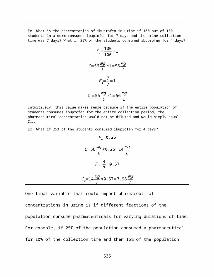
Figure S7. Comparison of global warming impacts (kg CO2 eq.) due to contributing processes (e.g., flush water, urine transport), generated emissions (e.g., nutrient discharge, pharmaceutical discharge), and avoided impacts (e.g., fertilizer offsets, brine incineration) in each scenario. The brackets around each error bar represent the 95% confidence interval resulting from Ecoinvent database distributions from the Monte Carlo uncertainty analysis.

S35

Figure S8. Comparison of smog impacts (kg O3 eq.) due to contributing processes (e.g., flush water, urine transport), generated emissions (e.g., nutrient discharge, pharmaceutical discharge), and avoided impacts (e.g., fertilizer offsets, brine incineration) in each scenario. The brackets around each error bar represent the 95% confidence interval resulting from Ecoinvent database distributions from the Monte Carlo uncertainty analysis.

S36

Figure S9. Comparison of acidification impacts (kg SO2 eq.) due to contributing processes (e.g., flush water, urine transport), generated emissions (e.g., nutrient discharge, pharmaceutical discharge), and avoided impacts (e.g., fertilizer offsets, brine incineration) in each scenario. The brackets around each error bar represent the 95% confidence interval resulting from Ecoinvent database distributions from the Monte Carlo uncertainty analysis.

S37

Figure S10. Comparison of eutrophication impacts (kg N eq.) due to contributing processes (e.g., flush water, urine transport), generated emissions (e.g., nutrient discharge, pharmaceutical discharge), and avoided impacts (e.g., fertilizer offsets, brine incineration) in each scenario. The brackets around each error bar represent the 95% confidence interval resulting from Ecoinvent database distributions from the Monte Carlo uncertainty analysis.

S38

Figure S11. Comparison of carcinogenic impacts (CTUh) due to contributing processes (e.g., flush water, urine transport), generated emissions (e.g., nutrient discharge, pharmaceutical discharge), and avoided impacts (e.g., fertilizer offsets, brine incineration) in each scenario. The brackets around each error bar represent the 95% confidence interval resulting from Ecoinvent database distributions from the Monte Carlo uncertainty analysis.

S39

Figure S12. Comparison of respiratory effects impacts (kg PM2.5 eq.) due to contributing processes (e.g., flush water, urine transport), generated emissions (e.g., nutrient discharge, pharmaceutical discharge), and avoided impacts (e.g., fertilizer offsets, brine incineration) in each scenario. The brackets around each error bar represent the 95% confidence interval resulting from Ecoinvent database distributions from the Monte Carlo uncertainty analysis.

S40

Figure S13. Comparison of fossil fuel depletion impacts (MJ surplus) due to contributing processes (e.g., flush water, urine transport), generated emissions (e.g., nutrient discharge, pharmaceutical discharge), and avoided impacts (e.g., fertilizer offsets, brine incineration) in each scenario. The brackets around each error bar represent the 95% confidence interval resulting from Ecoinvent database distributions from the Monte Carlo uncertainty analysis.

S41

S8. Impact of resin regeneration and brine incineration

Figure S14. Impact assessment results for methanol, sodium chloride, and potable water production used in the regeneration process (positive (+) percent contributions), compared to CO2 and NOx emission offsets, heavy fuel offsets, and hard coal offsets from incineration of the regeneration brine at a cement kiln plant (negative (–) percent contributions). The total bar length is equal to 100% of the impact within an impact category.

S42

S9. Impact of urine collection by vacuum truck and vacuum sewer

Figure S15. Normalized TRACI impact score (PE) of vacuum truck collection compared to the vacuum sewer collection as a function of vacuum sewer pipe length or distance traveled by vacuum truck (km).

S43

S10. Non-carcinogenic human toxicity impact

Figure S16. Comparison of non-carcinogenic human toxicity impact (CTUh = number of disease cases) due to (a) contributing processes (e.g., flush water, urine transport) and generated emissions (e.g., nutrients, pharmaceuticals) and avoided impacts (e.g., P offsets, N offsets) in each scenario and (b) pharmaceutical emissions only. The brackets around each error bar represent the 95% confidence interval resulting from Ecoinvent database distributions from the Monte Carlo uncertainty analysis.

S44

References

Alfonsín, C., Hospido, A., Omil, F., Moreira, M.T. and Feijoo, G. (2014) PPCPs in wastewater – Update and calculation of characterization factors for their inclusion in LCA studies. Journal of Cleaner Production 83, 245-255.Andersson, J., EKHEDEN, Y., KAJ, L., REMBERGER, M. and WOLDEGIORGIS, A. (2007) Results from the Swedish National Screening Programme, 2005. Subreport 1: Antibiotics, Anti-Inflammatory Substances, and Hormones.AWWA (2009) AWWA D103-09 Factory-Coated Bolted Carbon Steel Tanks for Water Storage.Bouatra, S., Aziat, F., Mandal, R., Guo, A.C., Wilson, M.R., Knox, C., Bjorndahl, T.C., Krishnamurthy, R., Saleem, F., Liu, P., Dame, Z.T., Poelzer, J., Huynh, J., Yallou, F.S., Psychogios, N., Dong, E., Bogumil, R., Roehring, C. and Wishart, D.S. (2013) The Human Urine Metabolome. PLoS ONE 8(9), e73076.Buchanan, J.R., Deal, N.E., Lindbo, D.L., Hanson, A.T., Gustafson, D. and Miles, R.J., Cost of Individual and Small Community Wastewater Management Systems: Wastewater Planning Model, version 1.0 (n.d.). Carollo Engineers (2012), Appedix P - Ozone Sizing and Cost Estimate for TORC Removal. http://www.cityofpaloalto.org/civicax/filebank/documents/32098Choe, J.K., Mehnert, M.H., Guest, J.S., Strathmann, T.J. and Werth, C.J. (2013) Comparative Assessment of the Environmental Sustainability of Existing and Emerging Perchlorate Treatment Technologies for Drinking Water. Environmental Science & Technology 47(9), 4644-4652.Edzwald, J.K. (2011) Water quality & treatment: a handbook on drinking water, McGraw-Hill New York.EPA (2012), Industrial & Municipal Waste Disposal Wells (Class I). http://water.epa.gov/type/groundwater/uic/wells_class1.cfmFDEP (2015) 2014 Reuse Inventory: Appendix D - Reclaimed Water Utilization.Fernandez-Fontaina, E., Omil, F., Lema, J.M. and Carballa, M. (2012) Influence of nitrifying conditions on the biodegradation and sorption of emerging micropollutants. Water Research 46(16), 5434-5444.FitzGerald, M.P., Stablein, U. and Brubaker, L. (2002) Urinary habits among asymptomatic women. American Journal of Obstetrics and Gynecology 187(5), 1384-1388.Forrest, A., Fattah, K., Mavinic, D. and Koch, F. (2008) Optimizing Struvite Production for Phosphate Recovery in WWTP. Journal of Environmental Engineering 134(5), 395-402.Fresh Water Systems (2016), Composite Well Tanks. https://www.freshwatersystems.com/c-35-composite-well-tanks.aspxGRU (2011) Biosolids Management Plan Update.Guishard, T. (n.d.), Comparisons of Steel Water Storage Tanks. http://timswatersolutions.com/pdf/2.pdfHauschild, M., McKone, T., Van de Meent, D., Huijbregts, M., Margni, M., Rosenbaum, R.K., Jolliet, O. and Fantke, P., USEtox 2.0 (2015). Hochmuth, G., Fan, J.H., Kruse, J. and Sartain, J. (2013), SL389/SS591: Using Reclaimed Water to Irrigate Turfgrass - Lessons Learned from Research with Nitrogen. University of Florida, https://edis.ifas.ufl.edu/ss591Hollender, J., Zimmermann, S., Koepke, S., Krauss, M., McArdell, C., Ort, C., Singer, H., von Gunten, U. and Siegrist, H. (2009) Elimination of Organic Micropollutants in a Municipal

S45

Wastewater Treatment Plant Upgraded with a Full-Scale Post-Ozonation Followed by Sand Filtration. Environmental Science & Technology 43(20), 7862-7869.Holloway, K. and Green, T. (2003) Drug and Therapeutics Committees - A Practical Guide, World Health Organization.Houghton, G.W., Dennis, M.J., Rigler, E.D. and Parsons, R.L. (1984) Urinary pharmacokinetics of orally administered Ketoprofen in man. European Journal of Drug Metabolism and Pharmacokinetics 9(3), 201-204.Huber, M.M., Canonica, S., Park, G.-Y. and von Gunten, U. (2003) Oxidation of Pharmaceuticals during Ozonation and Advanced Oxidation Processes. Environmental Science & Technology 37(5), 1016-1024.Ishii, S.K.L. and Boyer, T.H. (2015) Life cycle comparison of centralized wastewater treatment and urine source separation with struvite precipitation: Focus on urine nutrient management. Water Research 79, 88-103.Jimenez, J., Bott, C., Love, N. and Bratby, J. (2015) Source Separation of Urine as an Alternative Solution to Nutrient Management in Biological Nutrient Removal Treatment Plants. Water Environ Res 87(12), 2120-2129.Johnston, A.E. and Richards, I.R. (2003) Effectiveness of different precipitated phosphates as phosphorus sources for plants. Soil Use and Management 19(1), 45-49.Joss, A., Keller, E., Alder, A., Gobel, A., McArdell, C., Ternes, T. and Siegrist, H. (2005) Removal of pharmaceuticals and fragrances in biological wastewater treatment. Water Research 39(14), 3139-3152.Khan, U. and Nicell, J.A. (2010) Assessing the risk of exogenously consumed pharmaceuticals in land-applied human urine. Water Science & Technology 62(6).Kohler (2016), Steward waterless urinal. http://www.us.kohler.com/Landry, K.A. and Boyer, T.H. (2013) Diclofenac removal in urine using strong-base anion exchange polymer resins. Water Research 47(17), 6432-6444.Landry, K.A., Sun, P., Huang, C.-H. and Boyer, T.H. (2015) Ion-exchange selectivity of diclofenac, ibuprofen, ketoprofen, and naproxen in ureolyzed human urine. Water Research 68(0), 510-521.Latini, J.M., Mueller, E., Lux, M.M., Fitzgerald, M.P. and Kreder, K.J. (2004) VOIDING FREQUENCY IN A SAMPLE OF ASYMPTOMATIC AMERICAN MEN. The Journal of Urology 172(3), 980-984.Lienert, J., Gudel, K. and Escher, B. (2007) Screening method for ecotoxicological hazard assessment of 42 pharmaceuticals considering human metabolism and excretory routes. Environmental Science & Technology 41(12), 4471-4478.Lindqvist, N., Tuhkanen, T. and Kronberg, L. (2005) Occurrence of acidic pharmaceuticals in raw and treated sewages and in receiving waters. Water Research 39(11), 2219-2228.Lugon-Moulin, N., Ryan, L., Donini, P. and Rossi, L. (2006) Cadmium content of phosphate fertilizers used for tobacco production. Agron. Sustain. Dev. 26(3), 151-155.Magiera, S., Hejniak, J. and Baranowski, J. (2014) Comparison of different sorbent materials for solid-phase extraction of selected drugs in human urine analyzed by UHPLC–UV. Journal of Chromatography B 958(0), 22-28.Margot, J., Kienle, C., Magnet, A., Weil, M., Rossi, L., de Alencastro, L.F., Abegglen, C., Thonney, D., Chèvre, N., Schärer, M. and Barry, D.A. (2013) Treatment of micropollutants in municipal wastewater: Ozone or powdered activated carbon? Science of The Total Environment 461–462, 480-498.

S46

methanex (2015), Methanex posts regional contract methanol prices for North America, Europe, and Asia. https://www.methanex.com/our-business/pricingMorais, S.A. (2014) Multimedia fate modelling and impact of pharmaceutical compounds on freshwater ecosystems.Muñoz, I., Rodríguez, A., Rosal, R. and Fernández-Alba, A.R. (2009) Life Cycle Assessment of urban wastewater reuse with ozonation as tertiary treatment: A focus on toxicity-related impacts. Science of The Total Environment 407(4), 1245-1256.National Center for Environmental Economics (2010), Guidelines for preparing economic analyses. U.S. Environmental Protection Agency, https://yosemite.epa.gov/ee/epa/eerm.nsf/vwAN/EE-0568-50.pdf/$file/EE-0568-50.pdfNemecek, T. and Kägi, T. (2007) Life cycle inventories of agricultural production systems, Data v2.0, Ecoinvent Centre, Zurich and Dubendorf.Nordin, A., Nyberg, K. and Vinnerås, B. (2009) Inactivation of Ascaris Eggs in Source-Separated Urine and Feces by Ammonia at Ambient Temperatures. Applied and Environmental Microbiology 75(3), 662-667.Ott, L. and Longnecker, M. (2004) A first course in statistical methods, Thomson-Brooks/Cole, Belmont, CA.PRé Consultants (2014), http://www.pre-sustainability.com/Remy, C. (2010) Life Cycle Assessment of conventional and source-separation systems for urban wastewater management. Ph.D. Dissertation, Technische Universität Berlin.Rice, J. and Westerhoff, P. (2015) Spatial and Temporal Variation in De Facto Wastewater Reuse in Drinking Water Systems across the U.S.A. Environmental Science & Technology 49(2), 982-989.Richardson, G. (1999) Bolted steel tanks, HDPE geomembrane linings.Rivera-Utrilla, J., Sánchez-Polo, M., Ferro-García, M.Á., Prados-Joya, G. and Ocampo-Pérez, R. (2013) Pharmaceuticals as emerging contaminants and their removal from water. A review. Chemosphere 93(7), 1268-1287.Ronteltap, M., Maurer, M. and Gujer, W. (2007) The behaviour of pharmaceuticals and heavy metals during struvite precipitation in urine. Water Research 41(9), 1859-1868.Rosal, R., Rodríguez, A., Perdigón-Melón, J.A., Petre, A., García-Calvo, E., Gómez, M.J., Agüera, A. and Fernández-Alba, A.R. (2010) Occurrence of emerging pollutants in urban wastewater and their removal through biological treatment followed by ozonation. Water Research 44(2), 578-588.Salgado, R., Marques, R., Noronha, J., Carvalho, G., Oehmen, A. and Reis, M. (2012) Assessing the removal of pharmaceuticals and personal care products in a full-scale activated sludge plant. Environmental Science and Pollution Research 19(5), 1818-1827.Santos, J.L., Aparicio, I. and Alonso, E. (2007) Occurrence and risk assessment of pharmaceutically active compounds in wastewater treatment plants. A case study: Seville city (Spain). Environment International 33(4), 596-601.Sawchuk, R., Maloney, J., Cartier, L., Rackley, R., Chan, K.H. and Lau, H.L. (1995) Analysis of Diclofenac and Four of Its Metabolites in Human Urine by HPLC. Pharmaceutical Research 12(5), 756-762.Seyler, C., Hellweg, S., Monteil, M. and Hungerbühler, K. (2005) Life Cycle Inventory for Use of Waste Solvent as Fuel Substitute in the Cement Industry - A Multi-Input Allocation Model (11 pp). The International Journal of Life Cycle Assessment 10(2), 120-130.

S47

Snyder, S.A., Gunten, U.V., Amy, G., Debroux, J. and Gerrity, D. (2014) Use of Ozone in Water Reclamation for Contaminant Oxidation, pp. 373-376.STI/SPFA (2016), Water Storage Tank Total Cost of Ownership. http://www.steeltank.com/FabricatedSteelProducts/FieldErectedWaterTanks/TotalCostofOwnershipfreeonlinetool/tabid/474/Default.aspxSugawara, Y., Fujihara, M., Miura, Y., Hayashida, K. and Takahashi, T. (1978) Studies on the fate of naproxen. II. Metabolic fate in various animals and man. Chem Pharm Bull (Tokyo) 26(11), 3312-3321.Taute, J.J., Sole, K.C. and Hardwick, E. (2013) Zinc removal from a base metal solution by ion exchange: process design to full-scale operation, The Southern African Institute of Mining and Metallurgy, White River, Mpumalanga, South Africa.Ternes, T.A. (1998) Occurrence of drugs in German sewage treatment plants and rivers. Water Research 32(11), 3245-3260.Townsend, T., Gustitus, S.A., Walsh, A. and Krause, M.J. (2015) Municipal Solid Waste Composition Study at the University of Florida 2014, University of Florida.Tsai, L.L. and Li, S.P. (2004) Sleep patterns in college students: gender and grade differences. Journal of Psychosomatic Research 56(2), 231-237.U.S. EPA (2016), WaterSense Labeled Flushing Urinals. https://www3.epa.gov/watersense/pubs/faq_lfu.htmlUdert, K., Larsen, T., Biebow, M. and Gujer, W. (2003) Urea hydrolysis and precipitation dynamics in a urine-collecting system. Water Research 37(11), 2571-2582.UF (2014a), Approved Calendar: 2014-2015 Academic Year. https://catalog.ufl.edu/ugrad/current/Pages/calendar1415.pdfUF (2015) Common Data Set 2014-2015. Florida, U.o. (ed), University of Florida.UF (2014b) Human Resources 2013-2014. Florida, U.o. (ed), Integrated Postsecondary Education Data System.US EIA (2016), State Electricity Profiles. http://www.eia.gov/electricity/state/USEIA (2015) U.S. Gasoline and Diesel Retail Prices.USGS (2015) Mineral Commodity Summaries 2015, pp. 134-135.Vinnerås, B. (2001), Feacal separation and urine diversion for nutrient management of household biodegradable waste and wastewater. Thesis, URL: http://pub.epsilon.slu.se/3817/1/vinneras_b_091216.pdf. Vinnerås, B., Nordin, A., Niwagaba, C. and Nyberg, K. (2008) Inactivation of bacteria and viruses in human urine depending on temperature and dilution rate. Water Research 42(15), 4067-4074.Walton, B. (2014), Price of Water 2014: Up 6 Percent in 30 Major U.S. Cities; 33 Percent Rise Since 2010 - Circle of Blue. Circle of Blue, http://www.circleofblue.org/2014/world/price-water-2014-6-percent-30-major-u-s-cities-33-percent-rise-since-2010/Water Softeners & Filters (2016), Water Softener Tanks. http://www.water-softeners-filters.com/water-softeners/softener-tanksWeber, D., Capello, C., Seyler, C., Kohler, A., Hellweg, S. and Hungerbuhler, K. (2006), Ecosolvent 1.0.1. ETH Zurich, http://www.sust-chem.ethz.ch/tools/ecosolventWHOCC (2013), ATC/DDD Index 2015. http://www.whocc.no/atc_ddd_index/Zinckgraf, B., Liebnitzky, C., Kruse, J. and Boyer, T.H. (2014) Nutrient recovery potential from stadium wastewater for use as turfgrass fertilizer. University of Florida Journal of Undergraduate Research 15(2), 4.

S48