NREL is a national laboratory of the U.S. Department of Energy, Office of Energy Efficiency and Renewable Energy, operated by the Alliance for Sustainable Energy, LLC.

S3D Direct Numerical Simulation: Preparation for the 10–100 PF Era

Ray W. Grout, Scientific Computing GTC 2012 May 15, 2012 Ramanan Sankaran ORNL

John Levesque Cray

Cliff Woolley, Stan Posey nVidia

J.H. Chen SNL

2

Key Questions

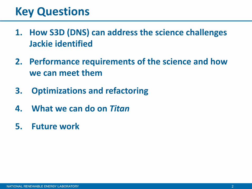
1. How S3D (DNS) can address the science challenges Jackie identified

2. Performance requirements of the science and how we can meet them

3. Optimizations and refactoring

4. What we can do on Titan

5. Future work

3

The Governing Physics

Compressible Navier-Stokes for Reacting Flows

• PDEs for conservation of momentum, mass, energy, and composition

• Chemical reaction network governing composition changes

• Mixture averaged transport model

• Flexible thermochemical state description (IGL)

• Modular inclusion of case-specific physics

- Optically thin radiation

- Compression heating model

- Lagrangian particle tracking

4

Solution Algorithm (What does S3D do?)

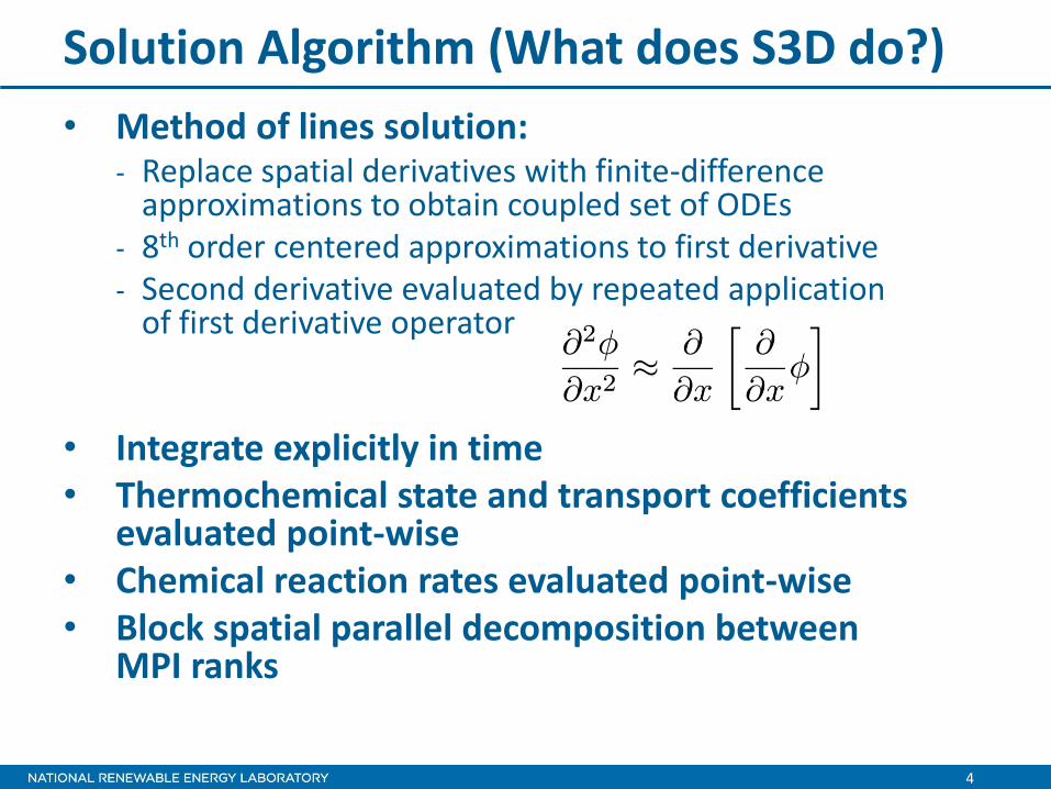
• Method of lines solution: - Replace spatial derivatives with finite-difference

approximations to obtain coupled set of ODEs - 8th order centered approximations to first derivative - Second derivative evaluated by repeated application

of first derivative operator

• Integrate explicitly in time • Thermochemical state and transport coefficients

evaluated point-wise • Chemical reaction rates evaluated point-wise • Block spatial parallel decomposition between

MPI ranks

5

Solution Algorithm

• Fully compressible formulation

– Fully coupled acoustic/thermochemical/chemical interaction

• No subgrid model: fully resolve turbulence-chemistry interaction

• Total integration time limited by large scale (acoustic, bulk velocity, chemical) residence time

• Grid must resolve smallest mechanical, scalar, chemical length-scale

• Time-step limited by smaller of chemical timescale or acoustic CFL

6

Resolution Requirements in Detail

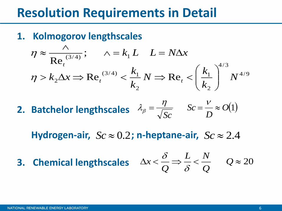
1. Kolmogorov lengthscales

2. Batchelor lengthscales

Hydrogen-air, ; n-heptane-air,

3. Chemical lengthscales

9/4

3/4

2

1

2

1)4/3(

2

1)4/3(

ReRe

;Re

Nk

kN

k

kxk

xNLLk

tt

t

1OD

ScSc

2.0Sc 4.2Sc

20 QQ

NL

Qx

7

Resolution Requirements (temporal)

1. Acoustic CFL

2. Advective CFL

3. Chemical timescale

- Flame timescale

- Species creation rates

- Reaction rates

- Eigenvalues of reaction rate jacobian

Mat

t

Mat

t

a

xt

u

a

u

a

L

cs

1max

iS

1max

j

8

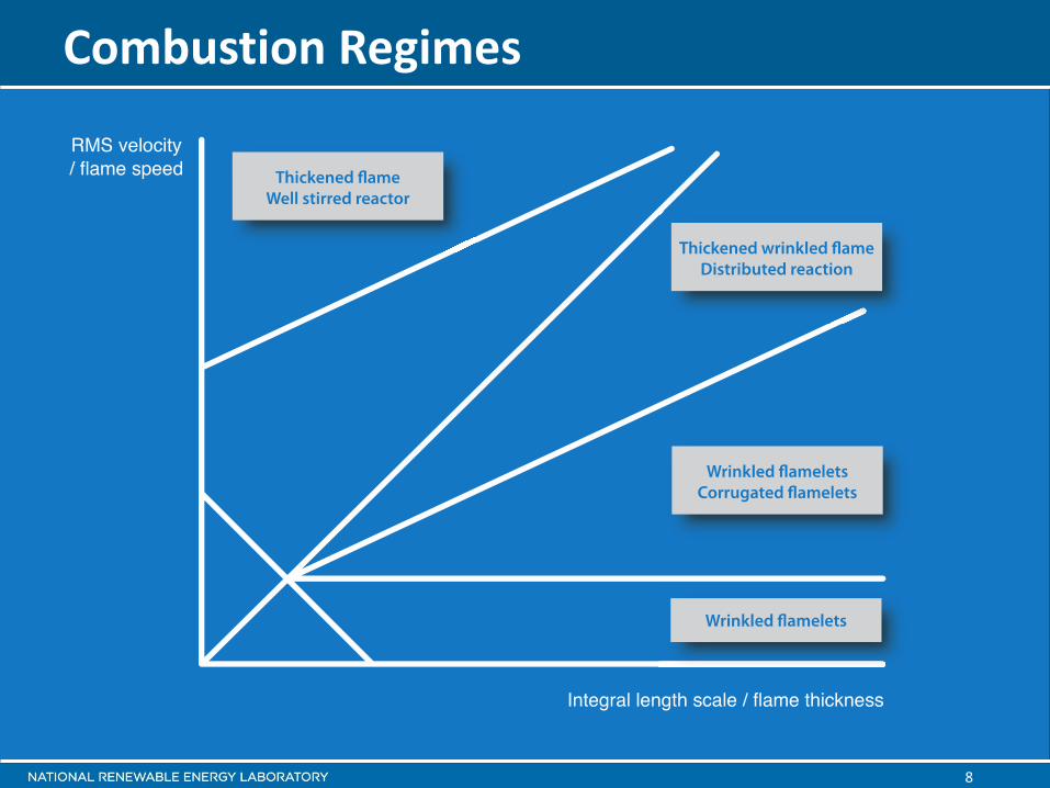
Combustion Regimes

9

Chemistry Reduction and Stiffness Removal

• Reduce species and reaction count through extensive static analysis and manipulation of reaction mechanism

• Literature from T. Lu, C.K. Law et al.

- DRG analysis of reaction network

- Quasi-steady state approximations

- Partial equilibrium approximations

• Dynamic analysis to adjust reactions that are assumed ‘fast’ relative to diffusion at runtime (implications later)

10

Benchmark Problem for Development

• HCCI study of stratified configuration

• Periodic

• 52 species n-heptane/air reaction mechanism (with dynamic stiffness removal)

• Mixture average transport model

• Based on target problem sized for 2B gridpoints

• 483 points per node (hybridized)

• 203 points per core (MPI-everywhere)

• Used to determine strategy, benchmarks, memory footprint

• Alternate chemistry (22 species Ethylene-air mechanism) used as surrogate for ‘small’ chemistry

11

Evolving Chemical Mechanism

• 73 species bio-diesel mechanism now available; 99 species iso-octane mechanism upcoming

• Revisions to target late in process as state of science advances

• ‘Bigger’ (next section) and ‘more costly’ (last section)

• Continue with initial benchmark (acceptance) problem

• Keeping in mind that all along we’ve planned on chemistry flexibility

• Work should transfer

• Might need smaller grid to control total simulation time

12

Target Science Problem

• Target simulation: 3D HCCI study

• Outer timescale: 2.5ms

• Inner timescale: 5ns ⇒ 500 000 timesteps

• As ‘large’ as possible for realism:

- Large in terms of chemistry: 73 species bio-diesel or 99 species iso-octane mechanism preferred, 52 species n-Heptane mechanism alternate

- Large in terms of grid size: 9003, 6503 alternate

13

Summary (I)

• Provide solutions in regime targeted for model development and fundamental understanding needs

• Turbulent regime weakly sensitive to grid size: need a large change to alter Ret significantly

• Chemical mechanism is significantly reduced in size from the full mechanism by external, static analysis to O (50) species

14

Performance Profile for Legacy S3D

Where we started (n-heptane) 242 × 16 720 nodes 5.6s

242 × 16 7200 nodes 7.9s

483 8 nodes 28.7s

483 18,000 nodes 30.4s

Initial S3D Code (15^3 per rank)

15

S3D RHS

16

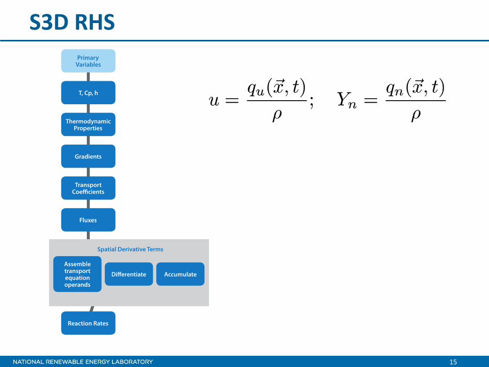
S3D RHS

Polynomials tabulated

and linearly interpolated

)();( 44 TphTpCp

17

S3D RHS

18

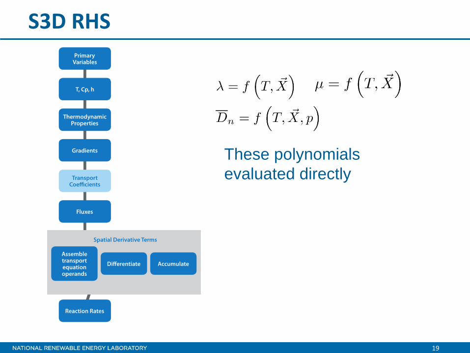
S3D RHS

Historically computed using sequential 1D derivatives

19

These polynomials

evaluated directly

S3D RHS

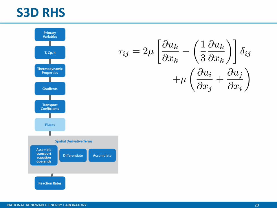
20

S3D RHS

21

S3D RHS

22

S3D RHS

23

Communication in Chemical Mechanisms

• Need diffusion term separately from advective term to facilitate dynamic stiffness removal - See T. Lu et al., Combustion and Flame 2009 - Application of quasi-steady state (QSS) assumption in situ - Applied to species that are transported, so applied by

correcting reaction rates (traditional QSS doesn’t conserve mass if species transported)

• Diffusive contribution usually lumped with advective term:

• We need to break it out separately to correct Rf, Rb

24

Readying S3D for Titan

Migration strategy: 1. Requirements for host/accelerator work distribution 2. Profile legacy code (previous slides) 3. Identify key kernels for optimization

- Chemistry, transport coefficients, thermochemical state (pointwise)

- Derivatives (reuse)

4. Prototype and explore performance bounds using cuda 5. “Hybridize” legacy code: MPI for inter-node, OpenMP

intra-node 6. OpenACC for GPU execution 7. Restructure to balance compute effort between accelerator

and host

25

Chemistry

• Reaction rate—temperature dependence - Need to store rates: temporary storage for Rf , Rb

• Reverse rates from equilibrium constants or separate set of constants

• Multiply forward/reverse rates by concentrations • Number of algebraic relationships involving non-contiguous

access to rates scales with number of QSS species • Species source term is algebraic combination of reaction

rates (non-contiguous access to temporary array) • Extracted as a ‘self-contained’ kernel; analysis by nVidia

suggested several optimizations • Captured as improvements in code generation tools

(see Sankaran, AIAA 2012)

26

Move Everything Over. . .

a For evaluating all gridpoints together

Memory footprint for 483 gridpoints per node

52 species n-Heptane 73 species bio-diesel

Primary variables 57 78

Primitive variables 58 79

Work variables 280 385

Chemistry scratch a 1059 1375

RK carryover 114 153

RK error control 171 234

Total 1739 2307

MB for 483 points 1467 1945

27

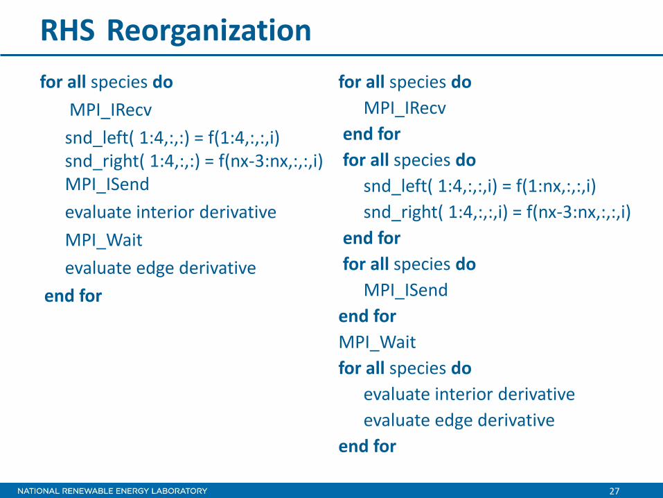
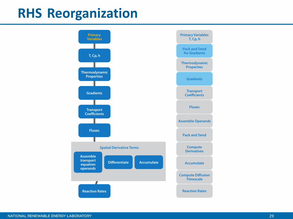
RHS Reorganization

for all species do

MPI_IRecv

snd_left( 1:4,:,:) = f(1:4,:,:,i) snd_right( 1:4,:,:) = f(nx-3:nx,:,:,i) MPI_ISend

evaluate interior derivative

MPI_Wait

evaluate edge derivative

end for

for all species do

MPI_IRecv

end for

for all species do

snd_left( 1:4,:,:,i) = f(1:nx,:,:,i)

snd_right( 1:4,:,:,i) = f(nx-3:nx,:,:,i)

end for

for all species do

MPI_ISend

end for

MPI_Wait

for all species do

evaluate interior derivative

evaluate edge derivative

end for

28

RHS Reorganization

29

RHS Reorganization

30

RHS Reorganization

31

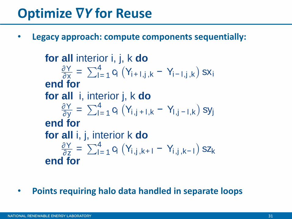
Optimize ∇Y for Reuse

• Legacy approach: compute components sequentially:

• Points requiring halo data handled in separate loops

NATIONAL RENEWABLE ENERGY LABORATORY 31 / 44

Optimize ∇ Y for reuse

— Legacy approach: compute components sequentially:

for all interior i, j, k do∂Y∂x =

4l= 1 cl Yi + l ,j ,k − Yi− l ,j ,k sx i

end forfor all i, interior j, k do

∂Y∂y =

4l= 1 cl Yi ,j + l ,k − Yl ,j − l ,k syj

end forfor all i, j, interior k do

∂Y∂z =

4l= 1 cl Yi ,j ,k+ l − Yi ,j ,k− l szk

end for

— Points requiring halo data handled in separate loops

32

Optimize ∇Y for Reuse

• Combine evaluation for interior of grid

• Writing interior without conditionals requires 55 loops

- 43, 42(N-8), 4(N-8)2,(N-8)3

NATIONAL RENEWABLE ENERGY LABORATORY 32 / 44

Optimize ∇ Y for reuse

— Combine evaluation for interior of grid

for all ijk doif interior i then

∂Y∂x =

4l= 1 cl Yi + l ,j ,k − Yi− l ,j ,k sx i

end ifif interior j then

∂Y∂y =

4l= 1 cl Yi ,j + l ,k − Yl ,j − l ,k syj

end ifif interior k then

∂Y∂z =

4l= 1 cl Yi ,j ,k+ l − Yi ,j ,k− l szk

end ifend for

— Writing interior without conditionals requires 55 loops

– 43, 42(N − 8), 4(N − 8)2, (N − 8)3 points

33

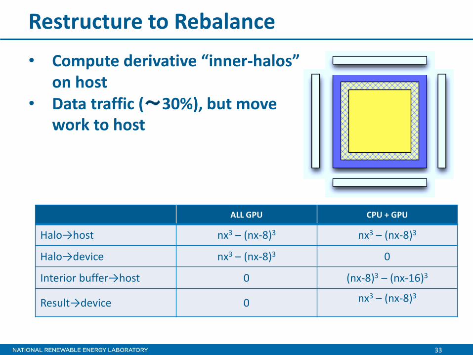
Restructure to Rebalance

• Compute derivative “inner-halos” on host

• Data traffic ( 30%), but move work to host

ALL GPU CPU + GPU

Halo→host nx3 – (nx-8)3 nx3 – (nx-8)3

Halo→device nx3 – (nx-8)3 0

Interior buffer→host 0 (nx-8)3 – (nx-16)3

Result→device 0 nx3 – (nx-8)3

34

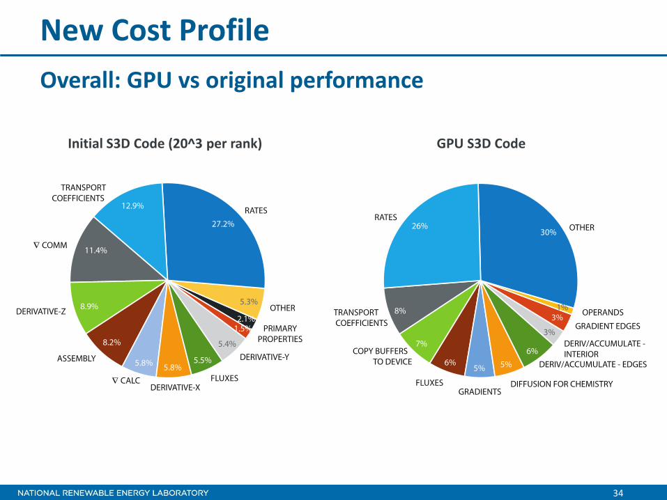
New Cost Profile

Overall: GPU vs original performance

Initial S3D Code (20^3 per rank) GPU S3D Code

35

Correctness

• Debugging GPU code isn’t the easiest… - Longer build times, turnaround - Extra layer of complexity in instrumentation code

• With the directive approach, we can do a significant amount of debugging using an OpenMP build

• A suite of physics based tests helps to target errors - ‘Constant quiescence’ - Pressure pulse / acoustic wave propagation - Vortex pair - Laminar flame propagation

– Statistically 1D/2D

36

Correctness

37

Summary (2)

• Significant restructuring to expose node-level parallelism

• Resulting code is hybrid MPI+OpenMP and MPI+OpenACC (-DGPU only changes directives)

• Optimizations to overlap communication and computation

• Changed balance of effort • For small per-rank sizes, accept degraded cache

utilization in favor of improved scalability

38

Reminder: Target Science Problem

• Target simulation: 3D HCCI study

• Outer timescale: 2.5ms

• Inner timescale: 5ns ⇒ 500 000 timesteps

• As ‘large’ as possible for realism:

- Large in terms of chemistry: 73 species bio-diesel or 99 species iso-octane mechanism preferred, 52 species n-Heptane mechanism alternate

- Large in terms of grid size: 9003, 6503 alternate

39

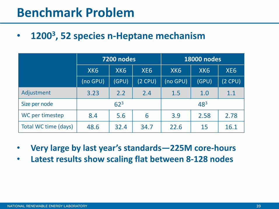
Benchmark Problem

• 12003, 52 species n-Heptane mechanism

• Very large by last year’s standards—225M core-hours • Latest results show scaling flat between 8-128 nodes

7200 nodes 18000 nodes

XK6 XK6 XE6 XK6 XK6 XE6

(no GPU) (GPU) (2 CPU) (no GPU) (GPU) (2 CPU)

Adjustment 3.23 2.2 2.4 1.5 1.0 1.1

Size per node 623 483

WC per timestep 8.4 5.6 6 3.9 2.58 2.78

Total WC time (days) 48.6 32.4 34.7 22.6 15 16.1

40

Time to Solution

Problem 7200 nodes 18000 nodes

CPU CPU+GPU CPU CPU+GPU

6503, 52 spc

Size per node 353

(6859, 6653) 253

(17576, 6503)

WC per timestep 1.5 1.0 0.55 0.36

Total WC time 8.8 5.8 3.2 2.1

9003, 52 spc

Size per node 463

(8000, 9203) 353

(17576, 9103)

WC per timestep 3.4 2.3 1.5 1.0

Total WC time 20 13 8.8 5.8

41

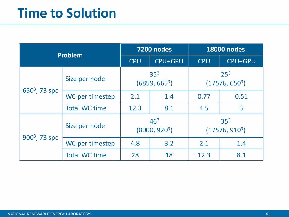
Time to Solution

Problem 7200 nodes 18000 nodes

CPU CPU+GPU CPU CPU+GPU

6503, 73 spc

Size per node 353

(6859, 6653) 253

(17576, 6503)

WC per timestep 2.1 1.4 0.77 0.51

Total WC time 12.3 8.1 4.5 3

9003, 73 spc

Size per node 463

(8000, 9203) 353

(17576, 9103)

WC per timestep 4.8 3.2 2.1 1.4

Total WC time 28 18 12.3 8.1

43

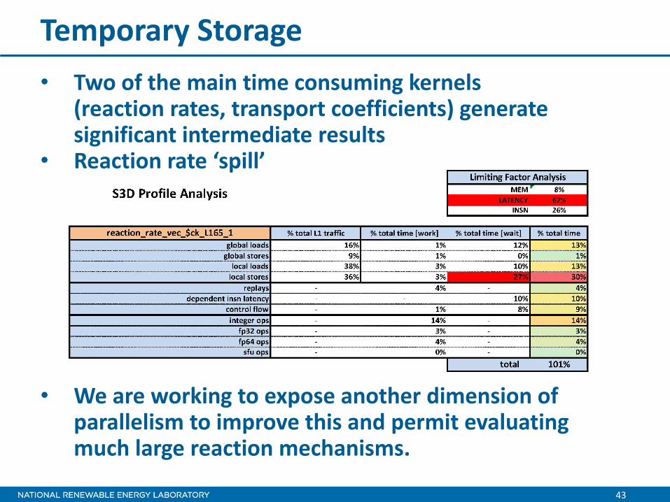
• Two of the main time consuming kernels (reaction rates, transport coefficients) generate significant intermediate results

• Reaction rate ‘spill’

• We are working to expose another dimension of

parallelism to improve this and permit evaluating much large reaction mechanisms.

Temporary Storage

44

Future Algorithmic Improvements

• Second Derivative approximation • Chemistry network optimization to minimize working

set size • Replace algebraic relations with in place solve • Time integration schemes—coupling, semi-implicit

chemistry • Several of these are being looked at by ExaCT

co-design center, where the impacts on future architectures are being evaluated - Algorithmic advances can be back-ported to this project

45

Outcomes

• Reworked code is ‘better’: more flexible, well suited to both manycore and accelerated - GPU version required minimal overhead using

OpenACC Approach - Potential for reuse in derivatives favors optimization

(chemistry not easiest target despite exps)

• We already have ‘Opteron + GPU’ performance exceeding 2 Opteron performance - Majority of work is done by GPU: extra cycles on CPU

for new physics (including those that are not well suited to GPU)

- We have the ‘hard’ performance - Specifically moved work back to the CPU

46

Outcomes

• Significant scope for further optimization - Performance tuning - Algorithmic - Toolchain - Future hardware

• Broadly useful outcomes • Software is ready to meet the needs of scientific

research now and to be a platform for future research - We can run as soon as the Titan build-out is complete . . .