Technical Report No. 46

SA C L A N T A S W

RESEARCH CENTRE

A COMPACT THERMOMETER FOR THE STUDY OF MICROTHERMAL

STRUCTURE FROM OCEANOGRAPHIC RUOYS

by

R PESARESI and R FRASSETTO

15 OCTOBER 1965

V I ALE SAN BART0L0ME0 . 92

l» SPEZIA, ITALY

ftDOiVH33l

TECHNICAL REPORT NO. 46

SACLANT ASW RESEARCH CENTRE

Viale San Bartolomeo 92

La Spezia, Italy

A COMPACT THERMOMETER FOR THE STUDY OF MICROTHERMAL

STRUCTURE FROM OCEANOGRAPHIC BUOYS

By

R. Pesaresi and R. Frassetto

15 October 1965

APPROVED FOR DISTRIBUTION

Director

TABLE OF CONTENTS

Page

ABSTRACT 1

INTRODUCTION 2

1. ELECTRONIC CIRCUIT 4

LI Working Principles 4

1.2 Actual Circuit 5

2. STAGGERING 8

2. 1 Principle 8

2. 2 Method of combining components 9

3. CIRCUIT STABILITIES AND SENSITIVITIES 12

3.1 Long term stability 12

3.2 Short-term stability 13

3.3 Temperature sensitivity 13

3.4 Pressure sensitivity 14

3. 5 Sensitivity to frequency of interrogation 15

3. 6 Sensitivity to power supply voltage 15

4. PHYSICAL CONSTRUCTION 16

CONCLUSIONS AND RECOMMENDATIONS 18

FIGURES 19

TABLES 27

A COMPACT THERMOMETER FOR THE STUDY OF MICROTHERMAL

STRUCTURE FROM OCEANOGRAPHIC BUOYS

By

R. Pesaresi andR. Frassetto

ABSTRACT

A solid-state, thermistor thermometer, of small physical size (13 cm xl4cm),

low cost (21 dollars worth of parts), and long-term stability (of the order

of 0. 01 C in 60 days) is described. It has been used successfully — in

vertical arrays — for the study of ocean thermal microstructure in turbulent

layers. Several probes can easily be plugged in on a 5 mm diam, single

conductor cable that also carries the load of a special, compact oceanographic

buoy. The electronic circuit is applicable to different types of sensor

(i.e. current velocity, direction meters and pressure gauges).

INTRODUCTION

A compact, oceanographic buoy system has been developed in this laboratory

for the study of turbulent layer structures in transitional areas of the ocean

where strong currents may be met. Sturdiness, small size, low cost and good

stability were the main characteristics desired for the sensors to be suspended

in vertical array from the buoy.

In this buoy system the sensors are required to make simultaneous meas-

urements at regular intervals over long periods of time, with minimum power

consumption. Among the various techniques for measuring, telemetering, and

recording oceanographic variables, the most suitable seemed to be that in

which a datum measurement is made proportional to a time interval between

two electric pulses. This is achieved by means of a compact circuit based

on an R-C timing network (the sensor providing the resistance) and a voltage

sensitive switch (a unijunction transistor).

With this technique, a. single conductor and sea return can be used. This

permits a simple installation, in which a large number of sensors can be

connected easily, both mechanically and electrically, to a single insulated

wire that also forms the taut mooring cable of the buoy.

Small size was obtained by the use of miniature components and printed

circuits, and by putting the circuits in epoxy resin that can be directly

exposed to hydrostatic pressures. The maximum pressure reached is

equivalent to a water column of 400 m. As measurements are to be made over

long periods of time, stability of the circuits is an important feature, and the

components have been properly selected and aged to achieve this. Among the

other characteristics that were looked for in the selection of components

from manufacturers' stocks was that of minimum sensitivity to external

pressure.

The buoy system is devised to permit the presentation of the pulse meas-

urements in a sequence corresponding to the sequence of the probes on the

array (first the shallowest, last the deepest). This is achieved by a

staggering technique, so that each probe has its own response time,

independent of the other probes. Enough pulse spacing is allowed to enable

temperature-inversions at any depth to be recognised.

ELECTRONIC CIRCUIT

1. 1 Working Principles

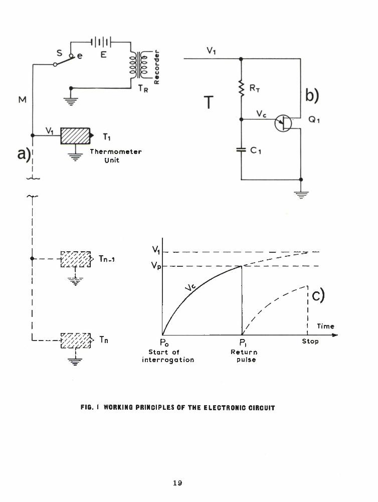
The working principles are illustrated in Fig. 1. Measurements are made

intermittently in cycles, each of which starts when switch S connects a

battery voltage E to the insulated mooring cable M and, hence, to the

array of thermometers T . . .T , (Fig. la). The initial surge of current

induces a voltage pulse P in the transformer T , across which a magnetic o R tape recorder is connected. The start of the cycle is thereby recorded as a

reference pulse from which all subsequent data pulses can be measured in

terms of their time intervals.

The thermometer probe circuits are based on relaxation oscillators employing

silicon unijunction transistors, as illustrated schematically in Fig. lb. When

the cycle starts, and battery voltage is applied to the cable, the voltage across

the capacitors Cl in each thermometer circuit T start to rise. As each

capacitor's voltage V reaches the level V (Fig. lc), its associated c p unijunction transistor Ql fires, Cl is discharged, and a return pulse P

is sent back along the cable to transformer T , where it induces a voltage R

pulse that is registered on the recorder.

For any one thermometer circuit, the time interval t between Pn and P x x is therefore the time taken for V to reach the level V , this being c p' » dependent on the resistance R of the thermistor. Thus, although all the

thermistor circuits start charging simultaneously, they send back independent

return pulses at time intervals t , t . . .t proportional to their ambient i i-i r_

temperatures. However, as will be explained in detail later, a staggering of

the time interval scale has been arranged so that there will be no confusion

when two thermometers are reading the same temperature, or when

reading temperatures through an inversion.

1.2 Actual Circuit

The complete circuit diagram is as shown in Fig. 2, which also shows the

circuits for three alternative probes: for pressure or current direction,

for temperature, and for current speed. These sensor circuits can be

connected, as indicated, to the input of the principal circuit shown on the left

of the figure, where their variable resistance is changed into a proportional

time interval between pulses. If the principal circuit was in the simple form

described in Para 1.1, and illustrated in Fig. lb, there would be nothing to

prevent the capacitor Cl from starting to recharge as soon as the transistor

Ql had fired. Thus, during all the time that battery voltage was applied to

the cable, there would be a continuous series of return pulses from the same

circuit. The complete circuit shown in Fig. 2 is designed to prevent this,

as well as to prevent each return pulse from triggering other circuits on the

same cable, to stabilize and filter the incoming battery voltage, and to prevent

the effects of sea water potentials and temperatures.

The diagram of the principal circuit is shown divided into two parts by broken

lines. That on the right corresponds to the simple form shown in Fig. lb,

except that it is Rl that carries the discharge pulse of Cl into Dl, and R2

compensates for the temperature sensitivity effects. The part on the left

includes all the other additions.

During operation, the return pulse P —arriving through Rl —triggers the

silicon controlled rectifier Dl, which in turn rapidly charges the capacitor

C2 through diode D3 and the external circuit.

During this process, the resistor R3 limits the current passing through

Dl to a value just above its "holding current"; this in turn is kept low by

the resistor R4. Thus, with Dl conducting, no further pulses from Ql

can reach the cable and be registered on the recorder.

A gate circuit, made up of diode D3 and resistor R5, prevents external

pulses from other thermometers on the cable from reaching Dl and

influencing its holding state. Similarly, the main thermistor circuit itself

is protected from these external pulses by the filter formed by resistor R7

and capacitor C3. The thermistor circuit is also kept reasonably independent

of supply voltage variations, sea water paths, sea water potentials, etc. by a

voltage stabilizing circuit made up of resistors R6 and R7 and the zener

diode D2.

At the end of each measurement cycle the switch S is open. In each

thermometer circuit all the capacitors are discharged first through the

emitter of the unijunction transistor 01, then through the resistances R

of the probe circuits, and hence through Rl, R2 and the R, . of the bb

transistor Ql. The rectifier Dl is then closed, making the circuit ready

for the next measurement cycle. The presence of the monel (used as common

return) in sea water acts as a weak battery, but diode D4 prevents this

charge from being received by capacitor Cl.

Figure 3 shows a complete measurement cycle, both in terms of the battery

voltage on the cable (upper graph) and in terms of the voltage across the

recorder side of transformer TR (lower graph). The pulses P,, P_, . . .P 12 n

from n thermometer circuits are shown; the temperature recorded by each

is proportional to the time interval (t,, t„, . . .t ) between its pulse and the 12 n

start pulse P . With the recording system at present in use it has been

found that a cycle lasting 6 sec provides the required resolution for 20

probes. The cycles can be repeated at any time intervals from 20 sec to

several minutes or hours, according to requirements.

2. STAGGERING

2. 1 Principle

The thermistors have a negative temperature coefficient; this means that with

decreasing temperature, their resistance — and the time response of the

thermometers described —will increase.

Therefore, if the temperature of the sea always decreased constantly with

depth (as in Fig. 4a), a group of matched thermometer circuits arranged

in parallel on an array would transmit their return pulses in the order of

their depth (Fig. 3). Sea temperature, however, does not continually decrease

with depth —isothermal layers (Fig. 4b) and temperature inversions

(Fig. 4c) are common. In isothermal water, matched thermometer circuits

would send back all their return pulses at the same time; in a temperature

inversion, the deeper thermometers (Y in Fig. 4c) would send back their

pulses before the shallower thermometers (X in Fig. 4c), and identification

would be impossible.

To avoid these difficulties a staggering method has been used, so that the

thermometers transmit their return pulses at progressively delayed times

according to their depth. Call At this preset interval between the return

pulses of adjacent thermometers on the array when they are reading identical

temperatures, and call S the sensitivity of the thermometer in sec/ C.

Then the value of At/S must be made greater than the maximum temperature

inversion expected between the thermometers, if the deeper is never to send

back its return pulse before the shallower. The value of At appropriate to

any given temperature inversion conditions is obtained by the proper selection

and combination of the thermometer circuit components.

The method of combining these different-sized components to obtain the

required degree of staggering will be discussed in the next chapter.

After assembly, the thermometers are calibrated and the degree of

staggering verified. Figure 5 shows a sample of calibration curves

and the values of 9 and At corresponding to one of them.

With the use of staggering it is no longer possible to use the same scale

for all thermometers when interpreting the intervals between pulses as

recorded temperatures. Instead, a separate scale is required for each

thermometer according to its calibration curve, but this can be accomplished

automatically by feeding the calibration data into the computer when the

final results are being analysed.

2. 2 Method of combining components

To obtain the required degree of staggering, slightly different values must

be used for each of the principal components — the thermistor, the capacitor

Cl, and the unijunction transistor. There is no need to buy special

components that differ by these small values, because such ranges are found

within the ranges of tolerance quoted by the manufacturers of standard

components. The standard components chosen were:

for the thermistors

for the Cl capacitors

for the unijunction transistors

Veco 51 A 11 100 k.Q

Tolerance of t 15% at 25°C

Mylar dielectric 15 jui, 60 v DC

Tolerance of t 10%

2N1671B Silicon

Tolerance of +- 20%

In the first production, 290 capacitors, 286 thermistors and 202

unijunction transistors were bought from manufacturers' standard stocks.

The frequency distribution of their deviations from quoted values was as

shown in Figs. 6a, b & c respectively. If components with greater

tolerance are selected, these distribution spreads can be increased and

the price of components decreased.

The combination of these components to obtain the desired degree of

staggering can be carried out by computer, but if a larger number of units

are being assembled at once, the possibilities become too great (for 100

units there are 10 combination possibilities). In such circumstances —

which would be the most usual — the quickest procedure is to combine the

capacitor and unijunction transistor as described below, and then to let the

computer combine these capacitor/unijunction transistor pairs with the 4

thermistors (this reduces the possibilities handled by the computer to 10

for 100 units).

To form the capacitor/unijunction transistor pairs, the individual

components are measured to within an accuracy of 1% and their values listed

in increasing order. The smallest-valued capacitor is then paired with the

smallest-valued transistor, and so on throughout the series. These pairs are

measured in combination with a known, stable resistor. The distribution of

values of the pairs is larger than the distribution of the capacitor of transistor

values (theoretically it is the sum of the two distribiitions:

t 10% for the capacitors plus t 20% for the unijunction transistors should

give a distribution of t 30% for the pairs). Figure 6d shows the result of

combining the capacitors and transistors that were used for Figs. 6a and 6c

respectively.

10

When the capacitor/transistor pairs are combined with the appropriate

thermistors, a large range of values is obtained from which all the

required degrees of stagger are possible.

11

CIRCUIT STABILITIES AND SENSITIVITIES

3. 1 Long term stability

Table A summarizes the differences between two calibrations made seventy

days apart. The estimated instrumental error ("t 5 m C) —which has to be

taken into account — is due to the time measuring system (automatic time

interval counter-printer) and the stability of the temperature bath (Fisher

isothemp bath).

The 18 thermometer circuits in Table A were used for field measurements

during twenty of the seventy days that separated the two calibrations. The

remaining fifty days are to be considered as shelf time.

These records refer to the first set of thermometers, made in 1963. However,

in 1964, another set was made in which the components used had not been aged.

Figure 7 compares the long-term stability of these two sets. Figure 7a shows

the percentage distribution of deviations recorded after 70 days with the 1963

(aged components) set; Figs. 7b & c show the percentage distributions of

deviations recorded after 270 and 98 days, respectively, with the 1964 (non-

aged components) set. In all three cases, the period between calibrations

included a period (from 15 to 30 days) of field use.

It is seen that — as is to be expected — the thermometers using aged

components are more stable (80% having a deviation within t 10 m C) than

those using non-aged components. However, it is also seen that natural ageing

occurs and that the stability during the second (98 day) period was proportionally

greater than during the first (270 day) period. This is expressed in Fig. 7d,

which compares the deviations of each individual thermometer during the two

12

periods. It is seen that 61% of the thermometers have a A"/A' relationship

between 0 and +1, indicating a decreasing degree of deviation in the second

period. Thus, especially if the deviations are acceptable for work during the

first two years use, thermometers could more easily be made with non-aged

components, as long as frequent calibrations are made during the early years.

3. 2 Short-term stability

Short-term stability of the circuits appears to be greater than the stability of

the measuring system. Table B gives the results of 20 measurements of 5

circuits, each made 5 min apart. Column (a) refers to thermometer circuits

incorporating thermistors, column (b) to the same thermometer circuits

where thermistors have been replaced by stable resistors.

The standard deviations ff and the differences A between the maximum

and minimum value measured are shown in each case. The differences in

values of both O and A between columns (a) and (b) are probably due to non-

homogeneities in the water of the calibration bath.

3. 3 Temperature sensitivity

The thermometer circuits (exclusive of thermistors) are to some extent

sensitive to temperature variations of the ambient. This is an effect of the

individual temperature sensitivities of the three components: transistor Ql,

capacitor Cl, and zener diode Dl (Fig. 2).

By varying the value of resistor R2 (Fig. 2) the temperature sensitivity of

the circuit can be reduced to some extent, within a given temperature range.

13

When a large number of components are involved, a statistical method must

be used to calculate this compensation. A sample of circuits is taken and

the values of R2 that minimize their temperature coefficients are measured.

The average of these values is then used for the whole batch of circuits.

However, before the batch of circuits is put into use, another sample is

taken and tested to ensure that the chosen value of R2 has given acceptable

results.

The sensitivity was found to be

which corresponds to

in the temperature range of 13 Oto 23 'C.

The time constant of the assembled circuits is about 3 min. Rapid ambient

temperature variations can therefore introduce an error in the measurements.

3. 4 Pressure sensitivity

The circuits are also sensitive to external pressure. The effect is felt

mostly by the main capacitor; miniature air bubbles trapped between the mylar

sheets decrease in volume and change its capacity.

14

Repeated pressure calibrations of the circuits, with a stable resistor

substituted for the variable resistance of the probe, showed that the effect

is different for each individual circuit but that calibration curves as a

function of pressure are repeatable, within a temperature error of _ 4 m C.

The pressure sensitivities were measured after a short time exposure (5 min) 2 to pressures of 10, 20, 30 and 40 kg/cm . Bey

the transistor and then the capacitor collapsed.

2 to pressures of 10, 20, 30 and 40 kg/cm . Beyond this latter pressure, first

Pressure sensitivities after long period of exposure exceeding two months

have not yet been measured.

3. 5 Sensitivity to frequency of interrogation

Capacitor Cl of the main circuit (Fig. 2a) takes a certain time to discharge

(average 20 sec) at the end of each cycle of interrogation. The next cycle can

begin only after Cl is completely discharged, if cumulative errors are to be

avoided.

So far, it has not been possible to increase the interrogation rate beyond 1 cycle

every 30 sec, at which rate the deviation is of the order of 0. 01 C. Means of

discharging Cl more rapidly are being investigated.

3. 6 Sensitivity to power supply voltage

The response time sensitivity to voltage variations is within t 0.2 m C/volt

at the normal voltage (24 v DC).

The maximum allowable deviation of 10 m C is reached below 18 v DC.

15

4. PHYSICAL CONSTRUCTION

Figure 8 shows the complete thermometer unit, as attached to the mooring

cable. It is 13 cm long and 4 cm diam.; in air it v/eighs 120 gm and in sea

water 60 gm.

The internal arrangements are shown in Fig. 9. The thermistor hid tube (1) is

embedded to half its length in a capped Vinyl tube (2) filled with Araldite.

The length by which it projects has been determined by tests, which show that

at least 1/2 cm of the glass root below the bid must be exposed to water for

effective heat dissipation. The bid is protected by a wire guard (3).

The Vinyl tube slides into a shock-absorbing rubber mounting (4) made in a

conical shape so that the bid has maximum, undisturbed exposure to the

current.

The thermistor is connected electrically to the rest of the circuit by flexible

wires long enough to permit several renewals of this fragile unit. The rest of

the circuit is potted in a PVC tube, into which the base of the rubber mount

fits; to take care of the different water compressions all the intervening

space is packed with Vaseline through the two buffer holes.

More than half of this tube is occupied by the main Mylar dielectric 15 >u f

capacitor (Cl in the circuit diagram), held in a central position by four

spacers. Below this are the remaining electronic components mounted on a

circular printed circuit. The base of the tube is closed by a neoprene

end-plate with a tapered wire protection. All the contents are potted in

Araldite.

16

Electrical connections between the thermometer unit and the recorder

are (1) through an electrical outlet on a single neoprene coated wire rope

of high tensile strength and good flexibility and (2) by a Monel sheet

riveted around the PVC tube, which acts as the conductor for sea return.

The deep-sea connector for the probe passes through a tapered neoprene

reinforcing sleeve.

These thermometer units have been exposed to mechanical and thermal

shocks and to vibrations of up to 100 cps without any change in their original

calibration curves.

Figure 8a and c show how the ground soldered contact is imbedded in the

Araldite to prevent exposure to water and galvanic corrosion.

17

CONCLUSIONS AND RECOMMENDATIONS

Over 100 thermometers have been made at the Centre and used for field

measurements from the Centre's oceanographic buoys for periods of from

15 to 30 days at a time. They have demonstrated that, with a few

improvements, the system is capable of recording temperature profiles

with an accuracy of - 0. 01 C.

A constant error was given by pressure, but a correction appropriate to the

working depth of each thermometer was applied before data processing. The

maximum depth for the electronics described in this report is 400 m.

However, it has been found that with long exposure to sea pressure — after

several periods of field work — the surrounding epoxy resin shows signs of

fatigue, as a result of which about 30% of the thermometers used in a recent

cruise (GIB V) were found to be shorted. It has therefore been decided to

enclose later models in stainless steel or titanium tubes closed by PVC end-

caps. This will keep the circuit at atmospheric pressure, and will also permit

further reduction in the size and weight of the probes, because components can

be chosen for their small size rather than for their lack of pressure-sensitivity.

Because of its temperature sensitivity, the circuit will then have to be potted

in a silicone compound within the metal tube. This will provide the greatest

possible thermal conductivity and thereby keep the circuit at the external

ambient temperature. If this is not done, there would be a risk of uncontrollable

errors when there are rapid temperature variations in the water.

Although the circuit described is designed for a 30 sec minimum interrogation

rate, it would require only the changing of a few critical components to make it

suitable for faster rates. In such a case, of course, the recording system

would have to be of a type that would permit adequate resolution.

18

T I

Thermometer Unit

I

-*//////?( Tn-1

__L_

I J- s ' ' / '/S tzsiA

i

Tn

Vi 1

Vp <L_-'_r"

L

/ / 1

/ 1 Time <- 1 •

Po Start of

interrogation

P. Return

pulse

Stop

FIG I WORKING PRINCIPLES OF THE ELECTRONIC CIRCUIT

19

g

I o

lN

LO Z

cr UJ . , o to

2 n

j

UJ a: 3 I/) LO UJ (X 0.

U Ul

oi , a :

n 6

CM

y

i if

i— :r\ fa >-=•

<M

I/)

UJ a

< cr UJ a.

UJ

a: O CO z Ul 10

a.

n

ro

——wv-

»tf —^v-

TU

-//-

c\j

u

©

4£

ioT

<J

K

I- a

O K U

_ J aiqDO 6UUOOIM

-fh

20

SWITCH'S CLOSES

E-

t 0 — rrvir

TIME

VOLTAGE ON THE CABLE

Po

START OF INTERROGATION

I

Pi P2 P» Pn-i Pn

_LJV LJLJJL RETURN PULSES

I 1

U-

1 I

tn.l- —tn- A \ 1

VOLTAGE ACROSS THE RECORDER TRANSFORMER

FIG. 3 COMPLETE MEASUREMENT CYCLE IN TERMS OF BOTH VOLTAGES

SURFACE

s

tr ui •- u

a < UJ I

777777777777777 BOTTOM

TEMP TEMP •»

B

TEMP

f 1

X

FIG. 4 MEASUREMENTS IN DIFFERENT WATER TEMPERATURE PROFILES

21

0) a E 0> I-

>

(/> c o a </>

a) E

o z

3 U

O -2

T

o . o

o

o o m n

o o o CO

•o c o o

0)

c o a </>

tr

0)

E

Ul >

o o CN

o o o CN

CN

o o CN

o

22

§30%

3 U o e -20 e

u e • I 10

290 CAPACITORS

15jif 60 v. DCWV±10% Mylar dielectric

B

D

io%-

c 3 o-

286 THERMISTORS VECO 51 A11-100KA±15%at25"C

tb. 14 12 10 8 -6 -4 -2 0 +2 +4 +6 8 10 12 14%

Deviation

£10% 3

202 2N 1671 B UNIJUNCTION

SILICON TRANSISTORS at Const, temp.

14 12 10 8 -6 -4 -2 0 +2 +4 +6 8 10 12 14% Deviation

?10%-

>< u c « 3 a

•*• 0

202 CAPACITORS • TRANSISTORS

14 12 10 8 -6 -4 -2 0 +2 +4 +6 8 10 12 14% Deviation

FIG. 6 FREQUENCY DISTRIBUTIONS OF DEVIATIONS FROM QUOTED VALUES

23

a)

60

40

20

0- •60 -40 -20

1963 Thermometers

A ^J-CJ

70 days

•20 *40 *60 *80

1964 Thermometers

b) 20-

1 1 i—i rH

270de i —1

lys

r» . 1 1 -60 -40 -20 • 20 *40 *60 *80

c)

40-

20-

A"= C3-C2

98 days

1 1 •60 -40 -20 >20 *40 *60 *80

d)

60 -

A" 40- A'

20-

0- i 1

i i

-2 -1 + 1 •2 *3 *4

FIG. 7 COMPARISON OF LONG-TERM STABILITY BETWEEN TWO SETS OF THERMOMETERS

24

FIG. 8 PHOTOGRAPH OF A COMPLETE THERMOMETER UNIT

^5

B

Thermistor

Vaseline

Arald ite or Ceramic

PVC Tube

Capacitor

Araldite or Ceramic

Circuit

Neoprene end Plate and Tapered Wire Protection

A Complete Probe

Thermistor Assembly

Ground

Stainless Steel Guard

eoprene Cap

Vinyl Tube

Neoprene Cone

Monel Sheet

VC Tube

Slot For Holding Monel Sheet in Place

Ground Connection Pro- tected From Sea Water

rinted Circuit

Araldite

Neoprene Insulated Wire

n 3 Mecca M 16 Female Deep Water Connector

Sea le

0 Centimetres

FIG. 9 THERMOMETER - CROSS SECTION VIEW

26

TABLE A

Long -term stability

CIRCUITS TEMPERATURE°C

N° 15° 17° 19° 21° 23° 25°

1 1.4 4.8 0 2.6 5.0 3.2

2 6.4 2.8 4.6 2.6 0 -7.2

3 -10.0 -7.4 -6.8 0.8 -0.8 0

4 -16.2 -14.6 -16.0 -14.8 -16.8 -12.4

5 4.8 12.6 8.6 7.6 9.8 12.2

6 1.8 6.0 5.8 4.0 5.4 6.8

7 21.4 26.6 26.8 28.4 29.4 34.4

8 -5.2 -2.8 -1.8 -0.6 -2.2 -3.4

9 20.4 14.4 13.4 12.8 9.6 9.0

10 -1.6 -0.4 -1.4 1.0 0 4.4

11 -8.6 -12.0 -13.4 -11.0 -10.2 -9.8

12 -0.6 0 1.2 5.8 2.8 5.2

13 -9.0 -8.2 -9.4 -9.8 -10.0 -9.2

14 1.2 2.4 2.6 2.8 8.2 9.2

15 -4.8 -8.2 -5.8 -8.4 -9.8 -3.8

16 6.4 6.6 9.6 6.8 3.4 9.0

17 0.4 3.6 2.8 4.2 5.2 6.6

18 -11.6 -9.6 -12.0 -8.2 -5.2 -6.6

Deviations in temperature readings after 70 days exhibited by a typical batch of thermometers (expressed in m°C±5m°C)

27

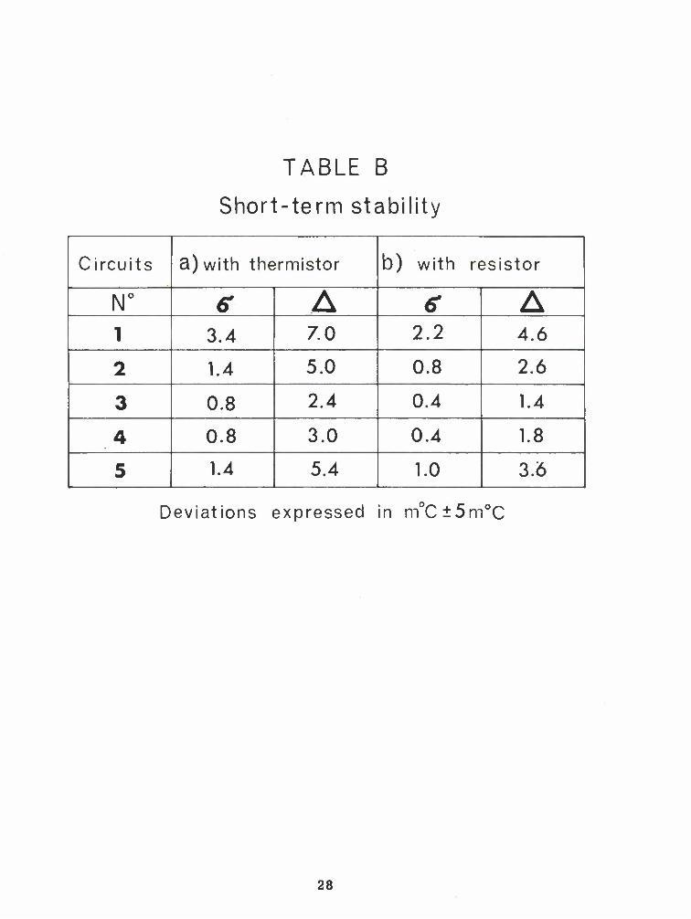
TABLE B

Short-term stability

Circuits a) with thermistor b) with resistor

N° e A 6* A 1 3.4 7.0 2.2 4.6

2 1.4 5.0 0.8 2.6

3 0.8 2.4 0.4 1.4

4 0.8 3.0 0.4 1.8

5 1.4 5.4 1.0 3.6

Deviations expressed in m°C±5m°C

28

DISTRIBUTION LIST

Minister of Defense Brussels, Belgium

Minister of National Defense Department of National Defense Ottawa, Canada

Chief of Defense, Denmark Kastellet CoDenhagen <b, Denmark

Minister of National Defense Division Transmissione-Ecoute-Radar 51 Latour Maubourg Paris 7e, France

10 copies

10 copies

10 cople

10 copies

Commander in Chief Western Atlantic Area (CINCWESTLANT) Norfolk 23511. Virginia

Commander In Chief Eastern Atlantic Area (CINCEASTLANT) Eastbury Park, Northwood Middlesex, England

Maritime Air Commander Eastern Atlantic Area (COMAIREASTLANT) R.A.F. Northwood Middlesex, England

1 copy

copy

1 copy

Minister of Defense Federal Republic of Germany Bonn, Germany

Minister of Defense Athens, Greece

Ministero della Difesa Stato Maggiore Marina Roma, Italy

Minister of National Defense Plein 4, The Hague, Netherlands

Minister of National Defense Storgaten 33, Oslo, Norway

Minister of National Defense Llsboa, Portugal

10 copies

10 copies

10 copies

10 copies

10 copies

10 copies

Commander Submarine Force Eastern Atlantic (COMSUBEASTLANT) Fort Blockhouse Gosport, Hants, England

Commander, Canadian Atlantic (COMCANLANT) H. M.C. Dockyard Halifax, Nova Scotia

Commander Ocean Sub-Area (COMOCEANLANT) Norfolk 23511, Virginia

Supreme Allied Commander Europe (SACEUR) Paris, France

SHAPE Technical Center P.O. Box 174 Stadhouders Plantsoen 15 The Hague. Netherlands

1 copy

1 copy

1 copy

7 copies

1 copy

Minister of National Defense Ankara, Turkey 10 copies

Allied Commander in Chief Channel (CINCCHAN) Fort Southwick, Fareham Hampshire, England 1 copy

Minister of Defense London, England

Supreme Allied Commander Atlantic (SACLANT) Norfolk 23511, Virginia

SACLANT Representative in Europe (SACLANTREPEUR) Place du Marechal de Lattre de Tasslgny Paris 16e, France

2<) copies

3 copies

1 copy

Commander Allied Maritime Air Force Channel (COMAIRCHAN) Northwood, England

Commander in Chief Allied Forces Mediterranean (CINCAFMED) Malta, G.C.

Commander South East Mediterranean (COMEDSOUEAST) Malta, G.C.

1 copy

1 copy

copy

Commander Central Mediterranean (COMEDCENT) Naples, Italy

Commander Submarine Allied Command Atlantic (COMSUBACLANT) Norfolk 23511, Virginia

Commander Submarine Mediterranean (COMSUBMED) Malta, G.C.

Standing Group, NATO (SGN) Room 2C256, The Pentagon Washington 25, DC.

Standing Group Representative (SGREP) Place du Marechal de Lattre de Tassigny Paris 16e, France

ASG for Scientific Affairs NATO Porte Dauphine Paris 16e, France

National Liaison Representatives

1 copy

1 copy

copy

3 copies

5 copies

copy

NLR Netherlands Netherlands Joint Staff Mission 4200 Linneau Avenue Washington, D.C. 20008

NLR Norway Norwegian Military Mission 2720 34th Street, N.W. Washington, D. C.

NLR Portugal Portuguese Military Mission 2310 Tracy Place, N.W. Washington, D.C.

NLR Turkey Turkish Joint Staff Mission 2125 LeRoy Place, N.W. Washington, D. C.

NLR United Kingdom British Defence Staffs, Washington 3100 Massachusetts Avenue, N.W. Washington, D.C.

NLR United States SACLANT Norfolk 23511, Virginia

1 copy

1 copy

1 copy

1 copy

1 copy

40 copies

NLR Belgium Belgian Military Mission 3330 Garfield Street, N.W. Washington, D.C.

NLR Canada Canadian Joint Staff 2450 Massachusetts Avenue, N.W. Washington, D.C.

1 copy

1 copy

Scientific Committee of National Representatives

Dr. W. l'etrie Defence Research Board Department of National Defence Ottawa, Canada copy

NLR Denmark Danish Military Mission 3200 Massachusetts Avenue, Washington, D.C. copy

G. Meunier Ingenieur en Chef des Genie Maritime Services Technique des Constructions et Armes Navales 8 Boulevard Victor Paris 15e, France 1 copy

NLR France French Military Mission 1759 "R" Street, N.W. Washington, D.C. copy

Dr. E. Schulze Bundesministerium der Verteidigung ABT H ROMAN 2/3 Bonn, Germany 1 copy

NLR Germany German Military Mission 3215 Cathedral Avenue, N.W. Washington, D.C. copy

Commander A. Pettas Ministry of National Defense Athens, Greece 1 copy

NLR Greece Greek Military Mission 2228 Massachusetts Avenue, N.W. Washington, D.C. copy

Professor Dr. M. Segreteria NATO MARIPERMAN La Spezia

Federici

1 copy

NLR Italy Italian Military Mission 3221 Garfield Street, N.W. Washington, D.C. 1 copy

Dr. M W. Van Batenburg Physisch Laboratorium RVO-TNO Waalsdorpvlakte The Hague, Netherlands 1 copy

Mr. A.W. Ross Directorof Naval Physical Research Ministry of Defence (Naval) Bank Block Old Admiralty Building Whitehall. London S.W. 1 1 copy

Dr. J.E. Henderson Applied Physics Laboratory University of Washington 1013 Northeast 40th Street Seattle 5, Washington 1 copy

Capitaine de Fregate R. C. Lambert Etat Major General Force Navale Caserne Prince Baudouin Place Dailly Bruxelles, Belgique 1 copy

CAPT H. L. Prause S4vaernet8 Televaesen LergravaveJ 55 Copenhagen S1, Denmark 1 copy

Mr. F. Lied Norwegian Defense Research Establishment Kjeller, Norway 1 copy

tag. CAPT N. Berkay Seyir Ve HDR D CUBUKLU Istanbul, Turkey 1 copy

National Liaison Officers

Mr. Sv. F. Larsen Danish Defense Research Board Osterbrogades Kaserne Copenhagen (X Denmark 1 copy

CDR R. J. M. Sabatler EMM/TER 2 Rue Royale Paris 8e, France 1 copy

Capitano dl Fregata U. Gilli Stato Maggiore della Marina Roma, Italia 1 copy

LCDRJ.W. Davis, USN Office of Naval Research Branch Office, London Box 39, Fleet Post Office New York, N. Y. 09510 1 copy

CDR Jose E.E.C. de Ataide Instltuto Hydrografico Rua Do Arsenal Porta H-l Lisboa 2, Portugal 1 copy