The Office of Financial Research (OFR) Working Paper Series allows members of the OFR staff and their coauthors to disseminate preliminary research findings in a format intended to generate discussion and critical comments. Papers in the OFR Working Paper Series are works in progress and subject to revision. Views and opinions expressed are those of the authors and do not necessarily represent officialpositions or policy of the OFR or Treasury. Comments and suggestions for improvements arewelcome and should be directed to the authors. OFR working papers may be quoted withoutadditional permission.

Safe Assets as Commodity Money

Maya Eden World Bank and Office of Financial Research meden@worldbank.org

Benjamin Kay Office of Financial Research Benjamin.Kay@ofr.treasury.gov

15-23 | November 25, 2015

Safe Assets as Commodity Money∗

Maya Eden† Benjamin Kay‡

November 25, 2015

Abstract

This paper presents a model in which safe assets are systemic be-cause they are the medium of exchange for risky assets. Like commod-ity money, these assets are costly to produce and have some intrinsicvalue, resulting in (a) non-neutrality and (b) overproduction. Quanti-tatively, the welfare consequences of these inefficiencies depend on thecosts of producing safe assets, which can be inferred from the equilib-rium value of the liquidity premium. When the model is calibrated toplausible liquidity premia the resulting inefficiencies are not large.

∗The views and opinions expressed in this paper are solely the responsibility of theauthors and should not be interpreted as reflecting the official policy or position of theWorld Bank, the Office of Financial Research, or the U.S. Department of Treasury. Wethank Greg Duffee, as well as seminar participants at the World Bank and Office ofFinancial Research for their helpful comments and suggestions.†World Bank, Development Economics Research Group, Macroeconomics and

Growth Team; and visiting scholar at the Office of Financial Research. Contact:meden@worldbank.org.‡Office of Financial Research. Contact: Benjamin.Kay@treasury.gov.

1

1 Introduction

In the study of the recent financial crisis, many analogies have been drawn

between safe assets and money. A common view of the 2007-09 crisis is that

it was prompted by a contraction in the effective supply of money-like assets,

as various securities that were previously perceived as very safe and liquid

were instead perceived as risky, consequently becoming illiquid (Gorton and

Metrick (2012)).

The goal of this paper is to formalize the analogy between safe assets

and money. In particular, we argue that, since the production of safe assets

requires real resources and since safe assets carry coupon payments that are

valued regardless of their use as a medium of exchange, the appropriate

conceptual framework for understanding their properties is as commodity

rather than fiat money. Our model suggests two main implications: (a)

changes in the quantity of safe assets can have real effects on the quantity of

trading (even absent nominal rigidities), and (b) there is overproduction of

safe assets.

These inefficiencies associated with commodity money are often cited as

grounds for the superiority of a fiat currency (Barro (1979); Ritter (1995),

and Kiyotaki and Wright (1989)). In line with this criticism, our model

implies that the use of safe assets as a medium of exchange in financial

trading is inefficient. However, a quantitative interpretation of the model

suggests that these inefficiencies are not large. In particular, we show that

these inefficiencies are increasing in the costs of creating safe assets, which

can be inferred from the liquidity premium. Given plausible estimates of

the liquidity premium, our simulations suggest that large fluctuations in the

quantity of safe assets are associated with only minor changes in welfare, and

that there are only minuscule inefficiencies generated by the overproduction

of safe assets.

A corollary of this analysis is that the contraction in the stock of safe

assets during the 2007-09 crisis is unlikely to be the direct cause of its sub-

2

sequent severity, at least not through the channels emphasized here. The

quantitative interpretation of our model suggests that the contraction in the

stock of safe assets was largely offset by an increase in the liquidity premium,

rather than by a contraction in the quantity of trading. In fact, while the

spike in liquidity premiums during the crisis was viewed by many as cause for

alarm, our model suggests that this equilibrium adjustment had an important

mitigating effect.

While there has been broad agreement in the literature that the analogy

between safe assets and money is potentially useful, there has been some

disagreement regarding the extent to which safe assets should be thought of

as “nominal balances” or as “real balances” (M and M respectively in stan-p

dard notation). For example, Stein (2012) and Krishnamurthy and Vissing-

Jorgensen (2012) consider money-in-the-utility-function models in which safe

assets enter the utility function directly, analogously to M . In contrast, Ro-p

cheteau and Wright (2013), Midrigan and Philippon (2011), Hart and Zin-

gales (2015) and Hart and Zingales (2011) consider models in which safe

assets are the medium of exchange, analogously to nominal balances. Our

paper clarifies the relationship between these two approaches.

This paper contributes to an emerging literature on the systemic im-

portance of safe assets, including Caballero (2006), Caballero et al. (2008),

Gourinchas and Jeanne (2012), Gorton and Ordonez (2013), and Dang et al.

(2012) (among others). Similar to Rocheteau and Wright (2013), Shen and

Yan (2014), Hart and Zingales (2011) and Hart and Zingales (2015), this

paper contributes to the discussion by studying the money-like properties

of safe assets. Most closely related are Hart and Zingales (2011) and Hart

and Zingales (2015). These papers highlight that when safe assets have a

transaction role, there is an oversupply of safe assets relative to the social

optimum. In this paper, we apply this insight to an environment in which

safe assets are used for facilitating trading in risky assets.

This paper is related to an extensive literature that studies pecuniary ex-

3

ternalities in constrained environments, such as Geanakoplos and Polemar-

chakis (1986), Greenwald and Stiglitz (1986), Caballero and Krishnamurthy

(2001), Lorenzoni (2008), Bianchi (2011), Farhi et al. (2009), Bengui (2013),

Korinek (2011) and Eden (ming) (among others). It is a well-established

principle that in the presence of binding constraints, a decentralized equilib-

rium may be inefficient due to inefficient price impacts on constrained agents.

This paper relates this principle to the inefficiency of private money creation

in an environment in which the cash-in-advance constraint is binding, and

draws implications regarding excessive private creation of safe assets.

Our modeling approach is motivated by important insights from the New

Monetarist view of liquidity (see Lagos et al. (2015) for a review). As illus-

trated by Lagos (2011), there is a theoretical equivalence between collateral

assets and assets used as a medium of exchange. In our model, we assume

that safe assets are used directly as a medium of exchange, building on this

equivalence for the broader interpretation of the model. While our approach

resembles a New Monetarist approach in some ways, there are also some dif-

ferences. In particular, our model departs from the assumption of bilateral

trading and assumes the presence of trading posts in which risky assets are

exchanged for the safe asset. This precludes the possibility that traders meet

by chance and choose to exchange one risky asset for another.1 We emphasize

that the aim of our paper is to apply and quantify insights from monetary

theory to the liquidity properties of safe assets, rather than to contribute to

the deep understanding of the foundations of the medium of exchange. For

this purpose, we adopt a framework that abstracts from multiple equilibria

and imposes the use of safe assets as a medium of exchange in risky assets.

1This trading structure appears realistic in the context of high-paced financial markets,in which the number of participants is large relative to the number of assets (thoughperhaps less so in the context of over-the-counter markets, as in Duffie et al. (2005)). Inaddition, it simplifies the analysis considerably, and generates results that are very muchin line with the more carefully microfounded models in the monetary literature.

4

2 Stylized facts

Before discussing the model, it is useful to illustrate some empirical regu-

larities that form the basis for the analogy between safe assets and money,

particularly around the crisis. This section cites some suggestive evidence

that safe assets provide liquidity services to the financial system, and that

the contraction in safe assets was associated with an increase in liquidity

premiums and a decline in trading volumes of illiquid assets.

Pozsar (2013) documents the critical role of safe assets like Treasury bills

(t-bills), commercial paper (CP), repurchase agreements (repos), and others

in institutional cash pools that are not fully counted in traditional money

supply aggregates like M2. Because of limits on Federal Deposit Insurance

Corporation (FDIC) insurance, holders of large quantities of cash cannot rely

on transaction accounts to store their liquid and transaction funds without

credit risk. Under their broader measure of money, classical M2 represents

only about half of the total. However, among institutional and securities

lender cash pools, non-M2 assets are about 80 percent of cash and cash

equivalents. While short term government debt is a significant source of

these non-depository safe assets, private actors, notably in shadow banking,

meet additional demand for safe assets through securitization and collateral

intermediation (Claessens et al. (2012)). During the financial crisis a signifi-

cant fraction of these privately manufactured liquid safe assets ceased to be

safe liquid assets (Gorton and Metrick (2012)) leading to significant increase

in the price of liquidity.

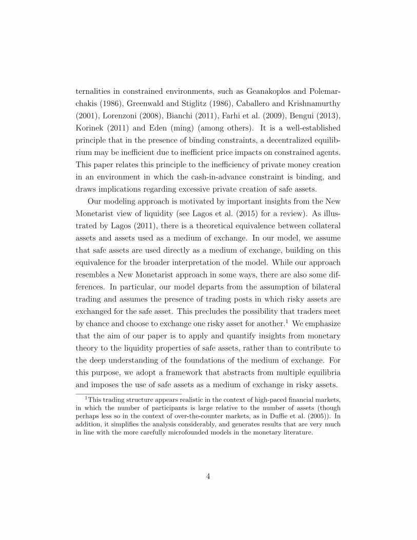
Figure 1 shows percentage of yield given up by on-the-run U.S. Treasury

holders over holding similar duration off-the-run securities. Since off-the-run

U.S. Treasuries are already more liquid than many assets, this premium ob-

served during the crisis is substantial given the actual liquidity difference.

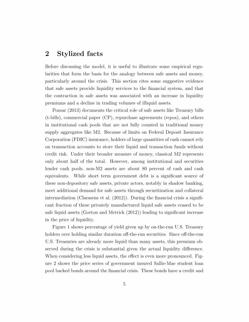
When considering less liquid assets, the effect is even more pronounced. Fig-

ure 2 shows the price series of government insured Sallie-Mae student loan

pool backed bonds around the financial crisis. These bonds have a credit and

5

interest rate risk very similar to U.S. Treasuries but are much less liquid. Dur-

ing the crisis these securities traded at about an 8 percent discount to par

and figure 2 documents that the remaining risks do not explain this discount,

suggesting illiquidity is the primary reason for depressed prices. Given these

pronounced premia over otherwise identical less-liquid safe assets, liquid safe

assets were in short supply in the financial crisis.

In addition to these large increases in liquidity premia in assets with

no credit risk, some markets for assets with credit risk froze up entirely in

the crisis. Hemmerdinger (2012) documents that auction-rate and short-

put bond origination declined precipitously as a result of the crisis. Radde

(2015) and Covitz et al. (2013) discuss the trading breakdown in repo, inter-

bank lending, and asset-backed commercial paper markets. Given the timing

coincident to so much asset market disorder, it is natural to wonder if safe

assets have an important role in facilitating the efficient trading of illiquid

assets and if the welfare losses from this illiquidity are large.

3 Model

This section presents a model in which safe assets are used as a medium of

exchange in risky assets. The model features traders with different prefer-

ences towards an evolving state of nature. Safe assets are valued similarly

by all agents. Though we will interpret the objects in our model as safe and

risky assets, it is worth emphasizing that the model also provides a general

treatment of economies in which an asset with real returns is used as the

medium of exchange.

Time is discrete and indexed t = 0, 1, .... There are n > 2 states of nature

indexed ω = 1, ..., n. States of nature occur with equal probabilities, and are

drawn independently across time.

There are n+1 assets, consisting of n risky assets indexed j = 1, .., n, and

one safe asset. The safe asset delivers 1 unit of the final good each period,

6

regardless of the state. The risky asset indexed j delivers one unit of the

final good in state ω = j, and nothing otherwise.2 The aggregate supplies

of the risky assets are denoted {Aj}nj=1, and the aggregate supply of the safe

asset is denoted As. Markets are incomplete in that all assets must be held

in weakly positive quantities.

There is a unit measure of traders of each type. Types are indexed i =

1, .., n, corresponding to the states of nature. A trader of type i values

consumption in state i more than in other states. Types are stochastic and

negatively correlated across time: a trader of type i at time t draws his t+ 1

type from {1, .., n} \ {i}, where each type occurs with equal probability. The

changes in types across time create a motive for trade in assets. The trader’s

preferences are described by:

U({ct, ωt, it}∞t=0) = Eωt,it

∞∑t=0

βtu(ct) (1 + θχωt=it)

[ ](1)

where ct is time t consumption, u(·) is an increasing and concave function

satisfying the Inada conditions, β ∈ (0, 1) is the discount factor, θ > 0 is a

preference parameter and χωt=it is an indicator function that takes a value 1

if ωt = it, and 0 otherwise.3 Traders are informed of their types one period in

advance: information on it+1 arrives at time t. Based on this information, the

traders may want to rebalance their asset portfolios. A trader’s “favorite”

risky asset corresponds to the asset aj such that it+1 = j; all other risky

assets will be referred to as “nonfavorite”.

We assume that risky assets are less liquid than safe assets, in the sense

that the markets for directly trading one risky asset for another are too

2To prevent agents from creating safe assets by bundling the n risky assets, it canbe assumed that there is an additional state, ω = n + 1, which occurs with negligibleprobability. Since there is no risky asset that delivers in state ω = n + 1 , a portfolio ofrisky assets cannot be used to create a safe asset.

3This specification of preferences is borrowed from the liquidity literature; see, forexample, Diamond and Dybvig (1983).

7

thin and do not open. Instead, trading takes place in n markets in which

risky assets are traded for the safe asset. Starr (2008) shows these money-

good bilateral markets can lead to the exclusion of good-good markets if

bilateral markets are costly to open. Hart and Zingales (2015) offer some

microfoundations for the emergence of safe assets as the medium of exchange.

Traders may enter each market only once during the trading period (either

as buyers or sellers). The safe asset therefore has a money-like quality, in

that it is assumed necessary for trading purposes. The trader allocates a

fraction γj of his safe assets for the purpose of buying risky assets of type j.

The price of risky assets of type j (in terms of safe assets) is denoted pj. It

is assumed for simplicity that dividends cannot be used for trading.4

Denote the trader’s holdings of assets of type j by aj, and his holdings

of safe assets by as. We assume that, in addition to dividends, each agent

receives a constant endowment of size e. In recursive form, the trader’s

problem can be written as follows:

V ({aj}nj=1, as, ω, i, i′, {pj}, e)

= max{a′j}nj=1,a

′s

u(c)(1 + θχω=i) + βEω′,i′′(V ({a′j}nj=1, a′s, ω

′, i′, i′′, {p′j}, e′))

(2)

s.t.

c =n∑j=1

ajχω=i + as + e (3)

n

j=1

γj ≤ 1∑

(4)

γj ≥ 0 (5)

pj(a′j − aj) ≤ γjas (6)

4Alternatively, we could also assume dividends are paid out after the markets close onholdings before markets open. In this sense, the period in our model where markets areopen the ex-dividend date.

8

a′s, a′j ≥ 0 (7)

a′s − as =n

j=1

pj(aj − a′j)∑

(8)

The trader’s value function, V (·), is a function of 2n + 5 state variables:

the initial holdings of each of the n risky assets ({aj}nj=1), their respective

market prices ({pj}), the initial holding of the safe asset (as), the state of

nature (ω), the agent’s endowment (e), the agent’s type, i, and the agent’s

type next period, i′. The trader consumes dividends and his endowment, and

re-optimizes his portfolio by choosing {a′j}nj=1 and a′s. During the trading

period, the trader can choose to allocate a fraction γj of his safe assets for

the purpose of buying the risky asset of type j. Equation 6 states that the

market value of assets of type j purchased by the trader must be less than

or equal to the amount of safe assets that he allocates for buying in market

j.

Equation 7 states that traders cannot hold negative amounts of assets.

Finally, equation 8 describes the evolution of the agent’s safe asset holding:

the left side is the net increase in safe assets, and the right hand side is net

the value of sales of risky assets.

Note that, in this framework, safe assets are valued independently from

their use as a medium of exchange: in addition to the liquidity services

that they provide (equation 6), they deliver returns in the form of dividends

(equation 3). The dividends associated with safe assets correspond, in a

standard monetary framework, to interest payments on money. In a model

of commodity money, these returns correspond to the consumption value of

the commodity (e.g., the utility from looking at shiny gold).

9

Welfare and efficiency. As a benchmark, it is useful to consider the effi-

cient allocation, defined as the solution to the following problem:

maxai,s,ai,j

n∑i=1

n∑i′=1

V ({ai,j}nj=1, ai,s, ω, i, i′, e) (9)

s.t. ni=1 i,j j i=1 i,s

In other words, the efficient allocation is achieved by a planner who assigns

equal Pareto weights to all agents and can allocate assets to traders depending

on their type. The efficient allocation allocates more consumption to agents

with i = ω. Specifically, it equalizes the marginal utility of consumption

across agents:

a = A and n a = As.∑ ∑

u′(c∗) = (1 + θ)u′(c̄∗) (10)

where c∗ is the allocation of consumption to agents with i = ω and c̄∗ is the

allocation of consumption to agents with i = ω.

For simplicity, we restrict attention to the case in which the above alloca-

tion cannot be achieved without all agents holding positive amounts of each

risky asset. Formally we assume that:

6

e+ As < c∗ (11)

The left hand side is the supply of safe assets, together with the endowment.

In a symmetric equilibrium, this will correspond to the non-state-contingent

dividends of all agents. If agents do not hold a positive amount of their

nonfavorite risky assets, this will be their consumption in their nonfavorite

state. The inequality states that in order to implement the efficient allocation

all agents must hold positive quantities of all risky assets.

For the purpose of welfare analysis, social welfare is given by equation 9.

10

Equilibrium. To define an equilibrium, index the set of traders by x ∈ X,

and let the set of trader x’s state variables be given by:

Sx = ({ax,j}nj=1, ax,s, ω, ix, i′x, {pj}nj=1, e)

A recursive equilibrium of this economy is given by policy functions a′x,j(Sx),

ax,s(Sx)′, γj(Sx) and prices p′j({Sx}x∈X) that jointly solve the trader’s opti-

mization problem and the market clearing conditions:∫X

(a′x,j(Sx)− ax,j)dx =

∫X

(a′x,s(Sx)− ax,s)dx = 0 (12)

The market clearing conditions state that the demand for each asset must

equal the supply of each asset; since there is no change in the aggregate

supply of assets, the aggregate changes in asset positions must be equal to 0.

Of course, by symmetry, there is an equilibrium in which pj = pi for all i

and j. We will focus on that symmetric equilibrium and sometimes omit the

subscript j (p = pj). Further, we will focus on a steady state equilibrium, in

which prices are constant across time (p = p′).

In a symmetric steady state, consumption depends on whether or not

the trader’s favorite state of nature has been realized. Denote equilibrium

consumption when i = ω by c̄ and equilibrium consumption when i = ω by

c.

The following proposition characterizes the symmetric steady state equi-

librium as a function of safe asset supply. For simplicity, we hold the efficient

allocation constant by assuming that E = e+As is constant (thus, a change

in As does not change the aggregate amount of goods in each state5):

6

Proposition 1 Assume that e+ As = E. Holding E constant:

1. For As sufficiently large, the steady state implements the efficient allo-

5That is, in a comparative statics sense, at this point As is exogenously determined.The next section will explore the consequences of exogenous and costly changes in As.

11

cation, and prices are given by pj = 1 .n

2. Otherwise, the efficient allocation is not implemented, and welfare is

increasing in As. Buyers are constrained: (1 + θ)u′(c̄) > u′(c). Safe

assets are associated with a liquidity premium, reflected in the fact that

p < 1 . Further, p and (u′ ′j j (c)− (1 + θ)u (c̄)) are increasing in As.

n

The proof is in Appendix A.

Proposition 1 establishes that when safe assets are scarce, increasing the

supply of safe assets increases trading volume and therefore equilibrium wel-

fare. The next section establishes that despite these benefits, there may be

excessive resources spent on the private creation of safe assets.

As an aside, it is worth emphasizing that when safe assets are sufficiently

abundant, the equilibrium implements the efficient allocation. Thus, this

model illustrates a potential advantage of commodity money (or safe assets)

over fiat money. While the literature suggests that the implementation of

the Friedman rule (Friedman (1969)) may not be feasible in an economy in

which fiat money is used as a medium of exchange (see ?, Wilson (1979), Cole

and Kocherlakota (1998) and Ireland (2003)), our model illustrates that it is

possible to satiate agents with liquidity given a form of commodity money

that is sufficiently abundant. Safe assets that pay dividends can be used in

the place of interest-bearing money to satiate the economy with liquidity,

effectively implementing the Friedman rule.

4 Creation of safe assets

This section extends the model to study the welfare implications of costly

private creation of safe assets. Consider a simple framework in which each

trader has a costly technology that transforms his endowment stream {e}∞t=0

into additional safe assets. For simplicity, assume that at t = −1 (before

trading begins), each agent can sacrifice a fraction γ of his endowment stream

12

to create εγ safe assets (where ε, γ ≤ 1). The trader’s problem at t = −1 can

be written as:

maxγ

Eω(V ({aj,0}nj=1, as,0 + εγe, ω, i, i′, {pj}, (1− γ)e)) (13)

We assume an interior solution in which traders transform part of their

illiquid endowment into safe assets (γ ∈ (0, 1)). The trader’s first order

condition with respect to safe asset creation is:

∂V

∂e= ε

∂V

∂as(14)

To characterize the solution to the above equation, it is useful to distinguish

between two cases. When ε = 1, it is costless to transform e into as; thus, in

equilibrium, the marginal benefit of as is the same as the marginal benefit of

e. In other words, there is no liquidity premium. In this case, by proposition

1, the efficient allocation is implemented and the economy is satiated with

liquidity.

If, instead, ε < 1, then the above equation can have a solution only when

there is a liquidity premium, e.g. only when safe assets are scarce.6 Absent

a positive liquidity premium, the trader would be indifferent between safe

assets and e, and since ε < 1, the trader would optimally set γ = 0. An

interior solution therefore implies a positive liquidity premium.

The above condition further illustrates how the cost of creating liquid

safe assets, ε, can be inferred from the liquidity premium. Intuitively, the

marginal benefit of liquid safe assets ( ∂V ) is equal to the marginal return to∂as

safe assets (∂V ), plus the liquidity benefits which are valued at the liquidity∂e

premium. In the quantitative interpretation of the model in the next section,

we will utilize the above relation to calibrate ε.

To evaluate the efficiency of the decentralized solution, consider next the

6This is analogous to the finding that private money creation is optimal only when theFriedman rule is not implemented, and there is some private seigniorage revenue associatedwith money creation.

13

problem of a social planner that can dictate to traders how many safe assets

to create. The planner’s t = −1 problem can be written as:

maxγ

Eω(n∑

i,i′=1

V ({aj,0}nj=1, as,0 + εγe, ω, i, i′, {pj}, (1− γ)e)) (15)

s.t. pj = p(As), where p(·) is a function mapping the aggregate supply of safe

assets to equilibrium prices (p). The difference between the planner’s problem

and the trader’s (decentralized) problem is that the planner internalizes that

an increase in the supply of safe assets may lead to a decline in the liquidity

premium (see Proposition 1).

The planner’s first order condition is:

∂V

∂e= ε

∂V

∂As= ε(

∂V

∂as+∂V

∂p

∂p

∂As) (16)

Note that the social return to safe assets ( ∂V ) is weakly lower than the∂As

private return to safe assets ( ∂V ). When there are sufficient safe assets,∂as

there is no liquidity premium associated with safe assets and the relative

price of risky and safe assets simply reflects the difference in expected asset

returns. In this case, ∂p = 0 and ∂V = ∂V .∂As ∂As ∂as

Otherwise, buyers of risky assets are constrained and ∂V < 0. It therefore∂p

follows that ∂V < ∂V , and there is excessive private creation of safe assets∂As ∂as

relative to the social optimum. This result is a consequence of a pecuniary

externality: when traders create safe assets, they do not internalize that an

increase in the supply of safe assets reduces the liquidity premium (raises

p). As buyers are constrained in each market, the increase in p worsens

equilibrium welfare.

It is useful to emphasize that there is no distortion when ε = 1. In this

case, the supply of safe assets is such that there is no liquidity premium,

and the economy is satiated with safe assets. In this case, ∂p = 0 and the∂As

planner’s solution coincides with the decentralized equilibrium allocation.

14

This benchmark suggests that when ε→ 1, the inefficiency due to excessive

private creation of safe assets approaches 0. In the following section, we will

argue that this is the empirically relevant case.

5 Quantitative interpretation

This section proposes a quantitative interpretation of the model, with two

goals in mind. The first is to quantify the degree of non-neutrality of safe

assets, or the real effects resulting from a large contraction in the stock of

safe assets. The second is to quantify the inefficiency due to excessive private

creation of safe assets.

The baseline model in Section 2 has five parameters: n, θ, Ar, As and e.

To calibrate the model, we normalize Ar = 1 and fix the number of states

(n) between 2 and 200,000. As it turns out, our results are not very sensitive

to the choice of n. Given Ar and n, we calibrate the remaining parameters

θ, As and e to match the following targets:

1. We match stock market trading volume or the “velocity” of safe assets.

In the model, assuming that As is below the saturation threshold level,

As trades hands in every trading round, in purchasing p(c̄ − c). Note

that As is the quantity of safe assets, not their value. The net present∑value of safe assets is ∞

t=0 βtAs = As

1− . We then define the tradingβ

volume as a fraction of GDP as:

tvs ≡As

(1− β)(Ar + e+ As)(17)

We target a pre-crisis tvs = 3.0 in line with Singh (2011).

2.1

The relative liquidity premium is defined as n − 1. To see this, notep

that when the liquidity premium is 0, p = 1 . If p is lower than 1 ,n n

it is valued at a positive premium. We target a liquidity premium

of 2 percent, in the range of values that Elmer (1999) estimates as

15

the value created by loan securitization as a percent of the original

balance.7 Alternatively, we could take as a liquidity premium the costs

of creating an Agency Mortgage-Backed-Securities (MBS). We estimate

these costs by adding the Fannie Mae and Freddie Mac guarantee fees

(Federal Housing Finance Agency (2014)) to the yield improvement

estimates of Sanders (2005) which amount to 0.5 percent of principal.

We choose the larger of the two estimates to give the liquidity channel

a greater chance to have an effect.

3. The share of safe assets out of total assets ( e+As ) is targeted at 1Ar+As+e 3

to match Gorton et al. (2010).

Using the equilibrium relationship in equation 14, we can then calibrate

ε as ε = ∂V / ∂V .∂e ∂as

The equilibrium is characterized by three endogenous variables: p, c̄ and c.

To solve for the equilibrium, we therefore rely on three equilibrium conditions.

The first is the goods market clearing condition: c̄+(n−1)c = n(Ar+As+e).

The second is an equilibrium condition stating that constrained traders spend

all of their safe assets on purchasing their favorite risky asset. The third

condition is obtained from the indifference of traders with respect to selling

their nonfavorite risky assets (equation 23 in the Appendix A). Appendix B

provides the details of the equations used for the simulation.

As a first exercise, we consider the implications of a 30 percent decline in

liquid safe assets, which is roughly in line with the share of asset backed se-

curities and mortgage backed securities in safe assets in Gorton et al. (2010).

To put the welfare consequences of a liquidity crisis in perspective we also cal-

culate a version of the model under autarchy (no-trade, constant symmetric

portfolios).

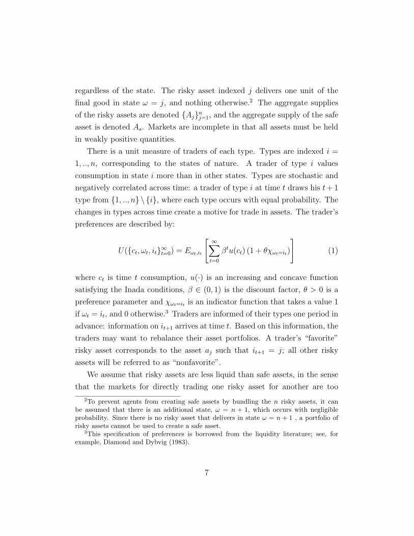
Figure 4 shows the basic result: both in absolute terms and relative to

the gains from trade, the losses from the liquidity crisis are small (regardless

7He estimates a range of 1.60-3.00 percent.

16

of the choice of n). For an n = 2 the welfare losses of the liquidity crisis are

14 percent of the gains over autarchy but as n increases they rapidly become

a de minimis fraction of the gains from trade.

We next consider the welfare loses from the overproduction of safe sassets.

Figure 4 shows that the losses are quantitatively small relative to autarchy

and the liquidity crisis. Normalizing the welfare losses by the liquidity crisis

losses indicates they are between 0.3 to 1.4 percent of crisis losses.

This quantitative interpretation highlights two striking features. First,

safe assets are approximately a neutral medium of exchange. Large changes in

the stock of safe assets lead to only minor changes in equilibrium allocations.

This is similar to fiat money in an environment in which money is neutral.

Second, while there is overproduction of safe assets, the inefficiency is not

large since the cost of producing safe assets is small. This too is similar to fiat

money, which is costless to produce. Furthermore, the low cost of production

results in an equilibrium allocation in which the economy is nearly satiated

with liquidity, similar to a monetary economy in which the Friedman rule is

implemented.

6 Conclusion

This paper makes several steps towards understanding the properties of safe

assets as a medium of exchange in financial trading. We show that while,

conceptually, the appropriate way to think about safe assets is as a form of

commodity money, in practical terms, they are quantitatively indistinguish-

able from fiat money in a model in which money is neutral. In particular, we

illustrate numerically that large changes in the quantity of safe assets result

in only small changes in equilibrium allocations and that, given empirically

relevant measures of the liquidity premium, safe assets appear to be nearly

costless to produce.

In fact, our analysis suggests that — perhaps unlike traditional forms

17

of commodity money - a monetary system that relies on safe assets as a

medium of exchange is relatively efficient. The fact that safe assets are

valued independently from their use as a medium of exchange means that,

when sufficiently abundant, the economy can be satiated with liquidity.

18

References

Barro, R. J. (1979). Money and the price level under the gold standard. The

Economic Journal , 13–33.

Bengui, J. (2013). Macro-prudential policy and coordination. Manuscript.

University of Montreal.

Bianchi, J. (2011, December). Overborrowing and systemic externalities in

the business cycle. American Economic Review 101 (7), 3400–3426.

Board of Governors (2015a). M2 money stock, monthly, seasonally adjusted

data in excel. https://research.stlouisfed.org/fred2/series/M2SL.

Board of Governors (2015b). The u.s. treasury yield

curve: 1961 to the present: Updated data excel file.

http://www.federalreserve.gov/econresdata/researchdata/feds200628.xls.

Caballero, R. J. (2006). On the macroeconomics of asset shortages. NBER

Working Paper 12753.

Caballero, R. J., E. Farhi, and P.-O. Gourinchas (2008). An equilibrium

model of global imbalances and low interest rates. American Economic

Review 98 (1), 358–393.

Caballero, R. J. and A. Krishnamurthy (2001). International and domestic

collateral constraints in a model of emerging market crises. Journal of

Monetary Economics 48 (3), 513–548.

Center for Financial Stability (2015). Divisia mon-

etary data for the united states data in excel.

http://centerforfinancialstability.org/amfm/Divisia Broad.xls.

Claessens, S., L. Ratnovski, and M. M. Singh (2012). Shadow banking: eco-

nomics and policy. Number 12. International Monetary Fund.

19

Cole, H. L. and N. Kocherlakota (1998). Zero nominal interest rates: Why

they’re good and how to get them. Federal Reserve Bank of Minneapolis

Quarterly Review 22, 2–10.

Covitz, D., N. Liang, and G. A. Suarez (2013). The evolution of a financial

crisis: Collapse of the asset-backed commercial paper market. The Journal

of Finance 68 (3), 815–848.

Dang, T. V., G. B. Gorton, and B. Holmstrom (2012). Ignorance, debt and

financial crises. Yale University and Massachusetts Institute of Technology,

Working Paper.

Diamond, D. W. and P. H. Dybvig (1983, June). Bank runs, deposit insur-

ance, and liquidity. Journal of Political Economy 91 (3), 401–419.

Duffie, D., N. Grleanu, and L. H. Pedersen (2005). Over-the-counter markets.

Econometrica 73 (6), 1815–1847.

Eden, M. (Forthcoming). Excessive financing costs in a representative agent

framework. American Economic Journal: Macroeconomics .

Elmer, P. J. (1999). Conduits: Their structure and risk. FDIC Banking

Review 12 (3), 27–40.

Farhi, E., M. Golosov, and A. Tsyvinski (2009). A theory of liquidity and

regulation of financial intermediation. Review of Economic Studies 76 (3),

973–992.

Federal Housing Finance Agency (2014, 11). Fannie Mae and Freddie Mac

Single-Family Guarantee Fees in 2013. Federal Housing Finance Agency.

Friedman, M. (1969). The optimum quantity of money. In The Optimum

Quantity of Money and Other Essays. Aldine Publishing Company.

20

Geanakoplos, J. D. and H. M. Polemarchakis (1986). Existence, regularity,

and constrained suboptimality of competitive allocations when the asset

market is incomplete. Uncertainty, information and communication: es-

says in honor of KJ Arrow 3, 65–96.

Gorton, G., S. Lewellen, and A. Metrick (2010). The safe asset share. Amer-

ican Economic Review, Papers and Proceedings 102, 101–106.

Gorton, G. and A. Metrick (2012). Securitized banking and the run on repo.

Journal of Financial economics 104 (3), 425–451.

Gorton, G. B. and G. L. Ordonez (2013). The supply and demand for safe

assets. NBER Working Paper No. w18732.

Gourinchas, P.-O. and O. Jeanne (2012). Global safe assets. BIS Working

Papers No 399.

Greenwald, B. and J. E. Stiglitz (1986). Externalities in economies with

imperfect information and incomplete markets. Quarterly Journal of Eco-

nomics 101 (2), 229–264.

Grkaynak, R. S., B. Sack, and J. H. Wright (2007). The u.s. treasury yield

curve: 1961 to the present. Journal of Monetary Economics 54 (8), 2291

– 2304.

Hart, O. and L. Zingales (2011). Inefficient provision of liquidity. NBER

working paper 17299.

Hart, O. and L. Zingales (2015). Liquidity and inefficient investment. Journal

of the European Economic Association.

Hemmerdinger, J. (2012, June 19, 2012). Variable- and auction-rate securities

dwindle. The Bond Buyer (August 2015).

Ireland, P. N. (2003). Implementing the friedman rule. Review of Economic

Dynamics 6, 120–134.

21

Kiyotaki, N. and R. Wright (1989). On money as a medium of exchange.

The Journal of Political Economy , 927–954.

Korinek, A. (2011). The new economics of prudential capital controls. IMF

Economic Review 59 (3), 523–561.

Krishnamurthy, A. and A. Vissing-Jorgensen (2012). The aggregate demand

for treasury debt. Journal of Political Economy 120 (2), 233–267.

Lagos, R. (2011). Asset prices, liquidity, and monetary policy in an exchange

economy. Journal of Money, Credit and Banking 43, 521–552.

Lagos, R., G. Rocheteau, and R. Wright (2015). Liquidity: A new monetarist

perspective. Journal of Economic Literature Forthcoming.

Lorenzoni, G. (2008). Inefficient credit booms. Review of Economic Stud-

ies 75 (3), 809–833.

Midrigan, V. and T. Philippon (2011). Household leverage and the recession.

No. w16965. National Bureau of Economic Research.

Pozsar, Z. (2013). Institutional cash pools and the triffin dilemma of the

us banking system. Financial Markets, Institutions & Instruments 22 (5),

283–318.

Radde, S. (2015). Flight to liquidity and the great recession. Journal of

Banking and Finance 54, 192–207.

Ritter, J. A. (1995). The transition from barter to fiat money. The American

Economic Review , 134–149.

Rocheteau, G. and R. Wright (2013). Liquidity and asset-market dynamics.

Journal of Monetary Economics 60 (2), 275–294.

Roy, M. (2015). Near-arbitrage among securities backed by government guar-

anteed loans.

22

Sanders, A. B. (2005). Measuring the benefits of fannie mae and freddie mac

to consumers: Between de minimis and small?

Shen, J. and H. Yan (2014). A search model of the aggregate demand for

safe and liquid assets.

Singh, M. (2011). Velocity of pledged collateral: analysis and implications.

IMF Working Papers , 1–24.

Starr, R. M. (2008). Commodity money equilibrium in a convex trad-

ing post economy with transaction costs. Journal of Mathematical Eco-

nomics 44 (12), 1413–1427.

Stein, J. (2012). Monetary policy as financial-stability regulation. Quarterly

Journal of Economics 127 (1), 57–95.

Wilson, C. (1979). An infinite horizon model with money. In J. S. J.R. Green

(Ed.), General Equilibrium, Growth, and Trade: Essays in Honor of Lionel

McKenzie. Academic Press, New York, NY.

A Proof of Proposition 1

To sustain an efficient equilibrium, it must be the case that buyers are in-

different with respect to purchasing an additional unit of their favorite risky

asset. For this to be the case, we must have that:

n− 1

nu′(c∗) +

1 + θ

nu′(c̄∗) + β

∂V ′

∂as=

1

p

1 + θ

nu′(c̄∗) + β

∂V ′

∂as(18)

The left hand side is the return from holding (and keeping) a safe asset.

Next period, the safe asset delivers a dividend with certainty; the marginal

valuation of that dividend is u′(c∗) whenever the realized state is ω = i, which6

23

occurs with probability n−1 , and (1+θ)u′(c̄∗) otherwise (with probability 1 ).n n

′The continuation value from holding the safe asset is β ∂V .

∂as

The right hand side is the return from using the safe asset to buy 1p

“favorite” risky assets, and then selling these assets in the next period in

exchange for a safe assets. A favorite risky asset delivers a dividend only

when the favorite state is realized, which occurs with probability 1 . In thatn

case, the marginal valuation of the dividend is (1 + θ)u′(c̄∗). The trader can

then sell his 1 risky assets for a safe asset, which delivers a continuation valuep

of β ∂V′. Note that the term β ∂V

′cancels out from both sides of equation

∂as ∂as

18. Further, note that, using equation 10, equation 18 can be rewritten as:

u′(c∗) =1

p

1

nu′(c∗)⇒ p =

1

n(19)

Note that, in this case, assets are priced according to their expected

value; there is no liquidity premium associated with safe assets. It is easy to

verify that, in this case, sellers of nonfavorite risky assets are indifferent with

respect to selling their nonfavorite asset in exchange for a safe asset. To see

this, note that the seller’s indifference condition is given by:

n− 1

nu′(c∗) +

1 + θ

nu′(c̄∗) + β

∂V ′

∂as=

1

p

1

nu′(c∗) + β

∂V ′

∂as(20)

The left hand side is the marginal benefit from selling 1 nonfavorite riskyp

assets in exchange for a safe asset, and the right hand side is the benefit from

holding 1 nonfavorite risky assets (and selling them in exchange for a safep

asset in the next period). Given equation 10, this indifference condition is

identical to equation 18.

To sustain this equilibrium, the supply of safe assets must be such that

the demand for risky assets can sustain the price p = 1 . In a symmetricn

steady state, buyers in the market for risky asset j consist of traders whose

favorite asset is j (and their favorite asset in the previous period was not j),

and sellers in the market consist of those whose favorite asset in the previous

24

period was j (and their favorite asset in the current period is not j). In

each market, buyers allocate at most As units of the safe asset towards the

purchase of their favorite risky assets. Note that sellers hold c̄ − c units of

asset j. Thus, in equilibrium, it must be the case that:

As ≥ p(c̄− c) =1

n(c̄∗ − c∗) (21)

If this inequality is violated, buyers do not hold enough purchasing power

to guarantee efficient holdings of their favorite risky assets. Thus, buyers

are constrained and (1 + θ)u′(c̄) > u′(c). The price p is such that sellers are

indifferent with respect to selling an additional unit of their nonfavorite asset

in exchange for a safe asset. The price p must satisfy the market clearing

condition:

As = p(c̄− c)⇒ p =As

c̄− c(22)

This equation defines a decreasing relationship between p and c̄− c.

∂V

∂as=n− 1

nu′(c) +

1 + θ

nu′(c̄) + β

∂V ′

∂as=

1

p(1

nu′(c) + βE(

∂V ′

∂aj|i) =

1

p

∂V

∂aj=i

(23)

6

′Where E(∂V |i) is the expected marginal valuation of holding asset j given

∂aj

type i = j. We claim that this equation defines an increasing relationship

between p and c̄ − c. When c̄ − c is higher, c is lower, implying a higher

marginal utility of consumption in the nonfavorite state. Given a higher

marginal utility of consumption, sellers require a higher price p in exchange

for an asset that delivers a return in their nonfavorite state. Thus, the seller’s

indifference condition defines an increasing relationship between p and c̄− c.Equation 22 defines a decreasing relationship between p and c̄−c, while 23

defines an increasing relationship between p and c̄− c. Thus, the equilibrium

is generated by their unique intersection. An increase in As shifts the curve

6

25

defined by equation 23 upwards, resulting in an equilibrium with higher p

and higher c̄− c. This concludes the proof.

B Simulation procedure

Note that buyers are constrained and (1 + θ)u′(c̄) > u′(c). The price p is

such that sellers are indifferent with respect to selling an additional unit of

their nonfavorite asset in exchange for a safe asset. The price p must satisfy

the market clearing condition:

As = p(c̄− c)⇒ p =As

c̄− c(24)

This equation defines a decreasing relationship between p and c̄− c.Indifference between the safe asset and selling the nonfavorite risky asset

at price p requires that:∂V

∂as=

1

p

∂V

∂aj=i6(25)

Note that ∂V b∂ s is given y the following expression, which is the expecteda

marginal utility of the safe asset in the next period plus its discounted con-

tinuation value:

∂V

∂as=n− 1

nu′(c) +

1 + θ

nu′(c̄) + β

∂V ′

∂as(26)

Note that 1 ∂V is given by:p ∂aj=i6

1

p

∂V

∂aj=i=

1

p(1

nu′(c) + βE(

∂V ′

∂aj|i)

6

′Where E(∂V |i) is the expected marginal valuation at time t of holding asset

∂aj

j at t+ 2, given type i = j at t+ 1.

This requires some manipulation to be in workable format:

6

26

Note that:∂V

∂e=n− 1

nu′(c) +

1 + θ

nu′(c̄) + β

∂V

∂e(27)

∂V

∂e=

1

1− β(n− 1

nu′(c) +

1 + θ

nu′(c̄)) (28)

Note that:

E(∂V ′

∂aj|i) =

1

n− 1

∂V

∂ai+n− 2

n− 1

∂V

∂aj=i6(29)

The trader’s next period’s type is chosen out of n−1 types that do not include

his current type. With probability 1− , the current nonfavorite asset becomesn 1

next period’s favorite asset; with probability n−2− it remains nonfavorite.n 1

The marginal valuation of a favorite asset is given by:

∂V

∂ai=

1 + θ

nu′(c̄) + β

∂V

∂aj=i6(30)

Combining the two:

E(∂V

∂aj|i) =

1

n− 1(1 + θ

nu′(c̄) + βE(

∂V

∂aj=i)) +

n− 2

n− 1

∂V

∂aj=i6 6(31)

⇒ E(∂V

∂aj|i) =

1 + θ

n(n− 1)u′(c̄) +

β + n− 2

n− 1E(

∂V

∂aj=i)

6(32)

Using the second line of equation 26,

1

nu′(c) + βE(

∂V ′

∂aj|i) =

∂V

∂aj=i6

Combining:

1

nu′(c) + β(

1 + θ

n(n− 1)u′(c̄) +

β + n− 2

n− 1E(

∂V

∂aj=i)) =

∂V

∂aj=i

1

nu′(c) + β

1 + θ

n(n− 1)u′(c̄) + β

β + n− 2

n− 1E(

∂V

∂aj=i) =

∂V

∂aj=i

6 6

6 6

27

1

nu′(c) + β

1 + θ

n(n− 1)u′(c̄) =

∂V

∂aj=i(1− ββ + n− 2

n− 1)

1nu′(c) + β 1+θ

n(n−1)u′(c̄)

1− β β+n−2n−1

=∂V

∂aj=i

6

6(33)

To calculate ∂V using the first line of equation 23, we need to calculate∂as

∂V ′ ∂V ′. Note that = ∂V , because the value of holding a unit of as at the

∂as ∂as ∂as

beginning of a period is different from the value of holding a unit of as at

the end of the period, after trading concludes. A safe asset at the beginning

of the period can be used to purchase 1 units of the favorite risky asset. Inp

the next period, it becomes a nonfavorite risky asset:

6

∂V ′

∂as=

1

p(1 + θ

nu′(c̄) + β

∂V

∂ai=j)

6(34)

The first line of equation 23 then yields:

∂V

∂as=n− 1

nu′(c) +

1 + θ

nu′(c̄) + β(

1

p(1 + θ

nu′(c̄) + β

∂V

∂ai=j))

6(35)

Then, equation 23 is an equation in c̄ and c (and parameters):

∂V 1 ∂V= ⇒

∂as p ∂aj=i6(36)

1 ∂V n− 1 1 + θ 1 1 + θ ∂V= u′(c) + u′(c̄) + β( ( u′(c̄) + β ))

p ∂aj=i n n p n ∂ai=j6 6(37)

1

p

∂V

∂aj=i(1− β2) =

n− 1

nu′(c) +

1 + θ

nu′(c̄)(1 +

β

p)

6(38)

∂V

∂aj=i=pn−1

nu′(c) + 1+θ

nu′(c̄)(p+ β)

1− β26(39)

Combining with equation 33:

28

pn−1nu′(c) + 1+θ

nu′(c̄)(p+ β)

1− β2=

1nu′(c) + β 1+θ

n(n−1)u′(c̄)

1− β β+n−2n−1

Together with the market clearing condition and As = p(c̄ − c) we have

three equations in three unknowns (p, c̄ and c). Because the calibration of

turnover and velocity are to flows measured in years we choose β = 0.97

corresponding to an annual discount rate. For each n we choose a θ and

fraction of all safe assets (Ysafe ≡ As + e) that are liquid ( As ≡ s̄ to satisfyYsafe

the pre-crisis calibration requirements. The calibration is simplified because

s̄ does not depend on n or θ.

(40)

tvs =As

(1− β) · Y=

s̄ · Ysafe(1− β) · Y

→ s̄ =tvs(1− β)Y

Ysafe

=3.0 · (0.03) · 1.5

(41)

0.5= 0.27

29

Conditional on s̄ and the other parameters, we choose θ to hit the target

liquidity premium of 0.02. Figure 5 shows that this relationship between n

and θ is nearly linear (θ ' 0.105 · n).

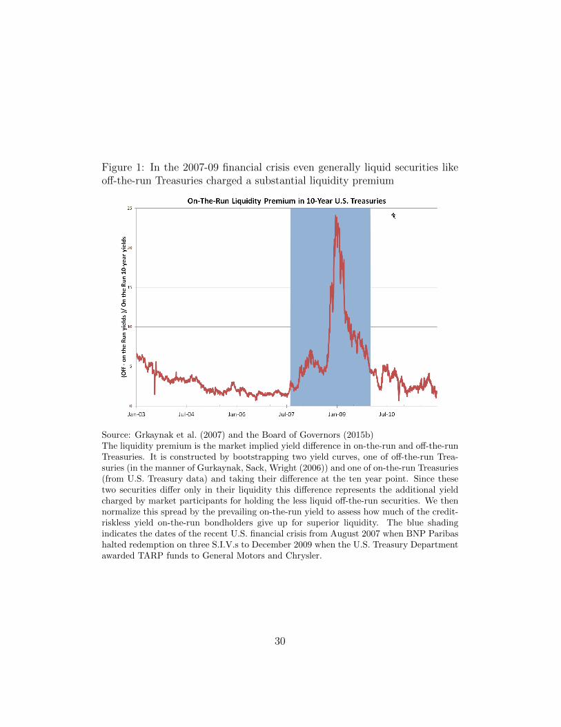
Figure 1: In the 2007-09 financial crisis even generally liquid securities likeoff-the-run Treasuries charged a substantial liquidity premium

Source: Grkaynak et al. (2007) and the Board of Governors (2015b)The liquidity premium is the market implied yield difference in on-the-run and off-the-runTreasuries. It is constructed by bootstrapping two yield curves, one of off-the-run Trea-suries (in the manner of Gurkaynak, Sack, Wright (2006)) and one of on-the-run Treasuries(from U.S. Treasury data) and taking their difference at the ten year point. Since thesetwo securities differ only in their liquidity this difference represents the additional yieldcharged by market participants for holding the less liquid off-the-run securities. We thennormalize this spread by the prevailing on-the-run yield to assess how much of the credit-riskless yield on-the-run bondholders give up for superior liquidity. The blue shadingindicates the dates of the recent U.S. financial crisis from August 2007 when BNP Paribashalted redemption on three S.I.V.s to December 2009 when the U.S. Treasury Departmentawarded TARP funds to General Motors and Chrysler.

30

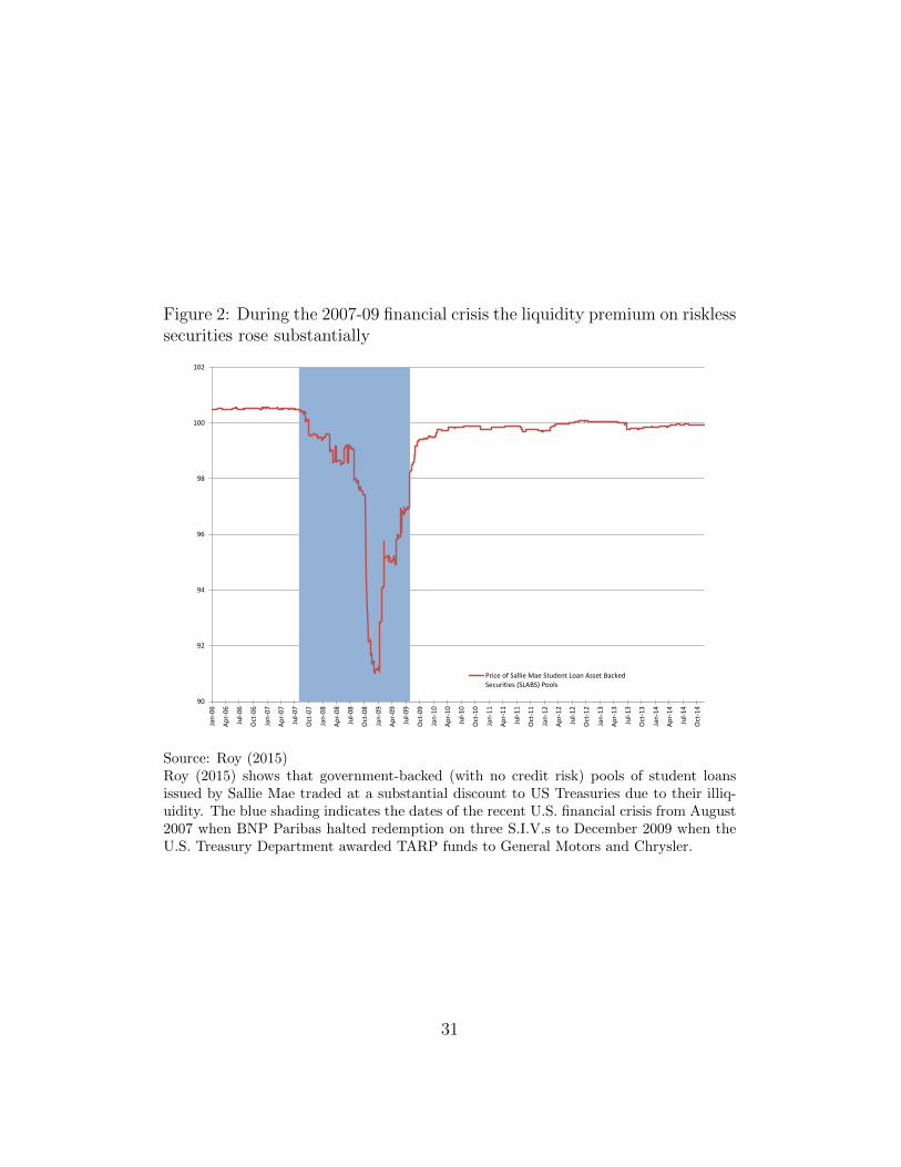
Figure 2: During the 2007-09 financial crisis the liquidity premium on risklesssecurities rose substantially

90

92

94

96

98

100

102

Jan-

06

Apr-

06

Jul-0

6

Oct

-06

Jan-

07

Apr-

07

Jul-0

7

Oct

-07

Jan-

08

Apr-

08

Jul-0

8

Oct

-08

Jan-

09

Apr-

09

Jul-0

9

Oct

-09

Jan-

10

Apr-

10

Jul-1

0

Oct

-10

Jan-

11

Apr-

11

Jul-1

1

Oct

-11

Jan-

12

Apr-

12

Jul-1

2

Oct

-12

Jan-

13

Apr-

13

Jul-1

3

Oct

-13

Jan-

14

Apr-

14

Jul-1

4

Oct

-14

Price of Sallie Mae Student Loan Asset BackedSecurities (SLABS) Pools

Source: Roy (2015)Roy (2015) shows that government-backed (with no credit risk) pools of student loansissued by Sallie Mae traded at a substantial discount to US Treasuries due to their illiq-uidity. The blue shading indicates the dates of the recent U.S. financial crisis from August2007 when BNP Paribas halted redemption on three S.I.V.s to December 2009 when theU.S. Treasury Department awarded TARP funds to General Motors and Chrysler.

31

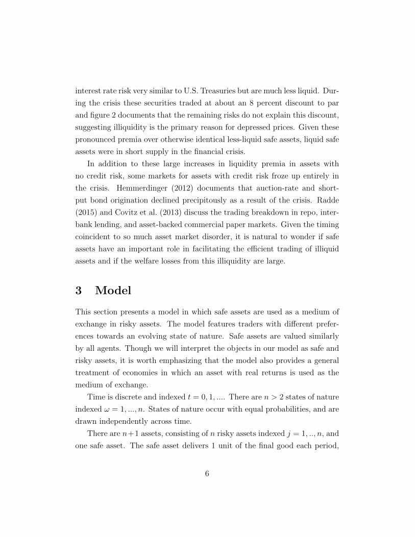
Figure 3: A contraction in money substitutes during the crisis

-0.1

-0.05

0

0.05

0.1

0.15

Jan-00 Jan-01 Jan-02 Jan-03 Jan-04 Jan-05 Jan-06 Jan-07 Jan-08 Jan-09 Jan-10 Jan-11 Jan-12 Jan-13 Jan-14

YoY M4 Growth (broad money measure includinginstutional safe assets)

YoY M2 Growth (narrower money measure)

Source: Author’s analysis, Center for Financial Stability (2015), and the Board of Gover-nors (2015a)Monthly growth rates (year-over-year) of a narrow monetary aggregate M2 (Board of Gov-ernors) and broader aggregate Divisia M4 (Center for Financial Stability) which includescommercial paper, U.S. Treasuries, and other assets used in money-like ways. The growthrate of the broader Divisia M4 fell faster and more severely than M2, contracting for overa year. The blue shading indicates the dates of the recent U.S. financial crisis from August2007 when BNP Paribas halted redemption on three S.I.V.s to December 2009 when theU.S. Treasury Department awarded TARP funds to General Motors and Chrysler.

32

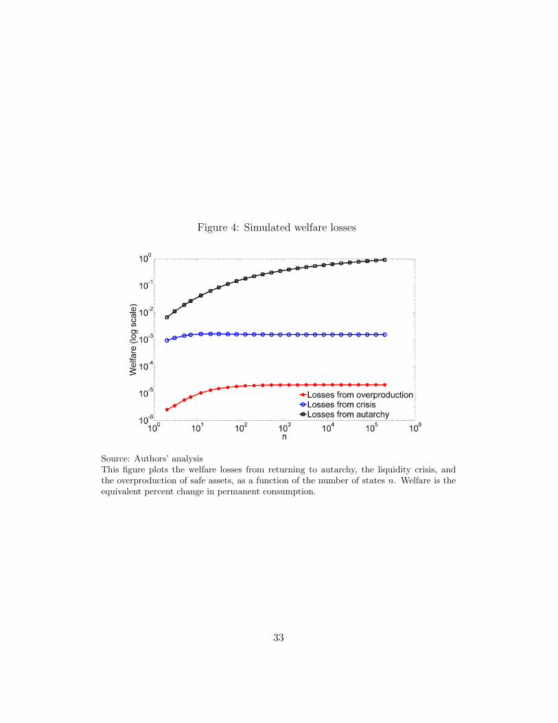
Figure 4: Simulated welfare losses

Source: Authors’ analysisThis figure plots the welfare losses from returning to autarchy, the liquidity crisis, andthe overproduction of safe assets, as a function of the number of states n. Welfare is theequivalent percent change in permanent consumption.

33

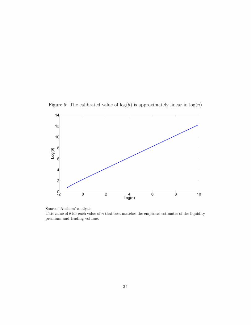
Figure 5: The calibrated value of log(θ) is approximately linear in log(n)

Source: Authors’ analysisThis value of θ for each value of n that best matches the empirical estimates of the liquiditypremium and trading volume.

34