sage reference manual: l-functions - sagemath...

Sage 9.1 Reference Manual:L-Functions

Release 9.1

The Sage Development Team

May 21, 2020

CONTENTS

1 Rubinstein’s 𝐿-function Calculator 3

2 Watkins Symmetric Power 𝐿-function Calculator 7

3 Dokchitser’s L-functions Calculator 11

4 Class file for computing sums over zeros of motivic L-functions. 19

5 Indices and Tables 29

Python Module Index 31

Index 33

i

Sage 9.1 Reference Manual: L-Functions, Release 9.1

Sage includes several standard open source packages for computing with 𝐿-functions.

CONTENTS 1


2 CONTENTS

CHAPTER

ONE

RUBINSTEIN’S 𝐿-FUNCTION CALCULATOR

This interface provides complete access to Rubinstein’s lcalc calculator with extra PARI functionality compiled in andis a standard part of Sage.

Note: Each call to lcalc runs a complete lcalc process. On a typical Linux system, this entails about 0.3 secondsoverhead.

AUTHORS:

• Michael Rubinstein (2005): released under GPL the C++ program lcalc

• William Stein (2006-03-05): wrote Sage interface to lcalc

class sage.lfunctions.lcalc.LCalcBases: sage.structure.sage_object.SageObject

Rubinstein’s 𝐿-functions Calculator

Type lcalc.[tab] for a list of useful commands that are implemented using the command line interface, butreturn objects that make sense in Sage. For each command the possible inputs for the L-function are:

• " - (default) the Riemann zeta function

• 'tau' - the L function of the Ramanujan delta function

• elliptic curve E - where E is an elliptic curve over Q; defines 𝐿(𝐸, 𝑠)

You can also use the complete command-line interface of Rubinstein’s 𝐿-functions calculations program viathis class. Type lcalc.help() for a list of commands and how to call them.

analytic_rank(L=”)Return the analytic rank of the 𝐿-function at the central critical point.

INPUT:

• L - defines 𝐿-function (default: Riemann zeta function)

OUTPUT: integer

Note: Of course this is not provably correct in general, since it is an open problem to compute analyticranks provably correctly in general.

EXAMPLES:

3

../../../../../../html/en/reference/structure/sage/structure/sage_object.html#sage.structure.sage_object.SageObject


sage: E = EllipticCurve('37a')sage: lcalc.analytic_rank(E)1

help()

twist_values(s, dmin, dmax, L=”)Return values of 𝐿(𝑠, 𝜒𝑘) for each quadratic character 𝜒𝑘 whose discriminant 𝑑 satisfies 𝑑min ≤ 𝑑 ≤ 𝑑max.

INPUT:

• s - complex numbers

• dmin - integer

• dmax - integer


OUTPUT:

• list - list of pairs (d, L(s,chi_d))

EXAMPLES:

sage: lcalc.twist_values(0.5, -10, 10)[(-8, 1.10042141), (-7, 1.14658567), (-4, 0.667691457), (-3, 0.480867558), (5,→˓ 0.231750947), (8, 0.373691713)]

twist_zeros(n, dmin, dmax, L=”)Return first 𝑛 real parts of nontrivial zeros for each quadratic character 𝜒𝑘 whose discriminant 𝑑 satisfies𝑑min ≤ 𝑑 ≤ 𝑑max.

INPUT:

• n - integer

• dmin - integer

• dmax - integer


OUTPUT:

• dict - keys are the discriminants 𝑑, and values are list of corresponding zeros.

EXAMPLES:

sage: lcalc.twist_zeros(3, -3, 6)-3: [8.03973716, 11.2492062, 15.7046192], 5: [6.64845335, 9.83144443, 11.→˓9588456]

value(s, L=”)Return 𝐿(𝑠) for 𝑠 a complex number.

INPUT:

• s - complex number


EXAMPLES:

4 Chapter 1. Rubinstein’s 𝐿-function Calculator


sage: I = CC.0sage: lcalc.value(0.5 + 100*I)2.69261989 - 0.0203860296*I

Note, Sage can also compute zeta at complex numbers (using the PARI C library):

sage: (0.5 + 100*I).zeta()2.69261988568132 - 0.0203860296025982*I

values_along_line(s0, s1, number_samples, L=”)Return values of 𝐿(𝑠) at number_samples equally-spaced sample points along the line from 𝑠0 to 𝑠1in the complex plane.

INPUT:

• s0, s1 - complex numbers

• number_samples - integer


OUTPUT:

• list - list of pairs (s, zeta(s)), where the s are equally spaced sampled points on the line from s0 tos1.

EXAMPLES:

sage: I = CC.0sage: lcalc.values_along_line(0.5, 0.5+20*I, 5)[(0.500000000, -1.46035451), (0.500000000 + 4.00000000*I, 0.606783764 + 0.→˓0911121400*I), (0.500000000 + 8.00000000*I, 1.24161511 + 0.360047588*I), (0.→˓500000000 + 12.0000000*I, 1.01593665 - 0.745112472*I), (0.500000000 + 16.→˓0000000*I, 0.938545408 + 1.21658782*I)]

Sometimes warnings are printed (by lcalc) when this command is run:

sage: E = EllipticCurve('389a')sage: E.lseries().values_along_line(0.5, 3, 5)[(0.000000000, 0.209951303),(0.500000000, -...e-16),(1.00000000, 0.133768433),(1.50000000, 0.360092864),(2.00000000, 0.552975867)]

zeros(n, L=”)Return the imaginary parts of the first 𝑛 nontrivial zeros of the 𝐿-function in the upper half plane, as 32-bitreals.

INPUT:

• n - integer


This function also checks the Riemann Hypothesis and makes sure no zeros are missed. This means itlooks for several dozen zeros to make sure none have been missed before outputting any zeros at all, sotakes longer than self.zeros_of_zeta_in_interval(...).

EXAMPLES:

5


sage: lcalc.zeros(4) # long time[14.1347251, 21.0220396, 25.0108576, 30.4248761]sage: lcalc.zeros(5, L='--tau') # long time[9.22237940, 13.9075499, 17.4427770, 19.6565131, 22.3361036]sage: lcalc.zeros(3, EllipticCurve('37a')) # long time[0.000000000, 5.00317001, 6.87039122]

zeros_in_interval(x, y, stepsize, L=”)Return the imaginary parts of (most of) the nontrivial zeros of the 𝐿-function on the line ℜ(𝑠) = 1/2 withpositive imaginary part between 𝑥 and 𝑦, along with a technical quantity for each.

INPUT:

• x, y, stepsize - positive floating point numbers


OUTPUT: list of pairs (zero, S(T)).

Rubinstein writes: The first column outputs the imaginary part of the zero, the second column a quantityrelated to 𝑆(𝑇 ) (it increases roughly by 2 whenever a sign change, i.e. pair of zeros, is missed). Higher upthe critical strip you should use a smaller stepsize so as not to miss zeros.

EXAMPLES:

sage: lcalc.zeros_in_interval(10, 30, 0.1)[(14.1347251, 0.184672916), (21.0220396, -0.0677893290), (25.0108576, -0.→˓0555872781)]

6 Chapter 1. Rubinstein’s 𝐿-function Calculator

CHAPTER

TWO

WATKINS SYMMETRIC POWER 𝐿-FUNCTION CALCULATOR

SYMPOW is a package to compute special values of symmetric power elliptic curve L-functions. It can compute upto about 64 digits of precision. This interface provides complete access to sympow, which is a standard part of Sage(and includes the extra data files).

Note: Each call to sympow runs a complete sympow process. This incurs about 0.2 seconds overhead.

AUTHORS:

• Mark Watkins (2005-2006): wrote and released sympow

• William Stein (2006-03-05): wrote Sage interface

ACKNOWLEDGEMENT (from sympow readme):

• The quad-double package was modified from David Bailey’s package: http://crd.lbl.gov/~dhbailey/mpdist/

• The squfof implementation was modified from Allan Steel’s version of Arjen Lenstra’s original LIP-basedcode.

• The ec_ap code was originally written for the kernel of MAGMA, but was modified to use small integers whenpossible.

• SYMPOW was originally developed using PARI, but due to licensing difficulties, this was eliminated. SYM-POW also does not use the standard math libraries unless Configure is run with the -lm option. SYMPOW stilluses GP to compute the meshes of inverse Mellin transforms (this is done when a new symmetric power is addedto datafiles).

class sage.lfunctions.sympow.SympowBases: sage.structure.sage_object.SageObject

Watkins Symmetric Power 𝐿-function Calculator

Type sympow.[tab] for a list of useful commands that are implemented using the command line interface,but return objects that make sense in Sage.

You can also use the complete command-line interface of sympow via this class. Type sympow.help() for alist of commands and how to call them.

L(E, n, prec)Return 𝐿(Sym(𝑛)(𝐸, edge)) to prec digits of precision, where edge is the right edge. Here 𝑛 must be even.

INPUT:

• E - elliptic curve

• n - even integer

• prec - integer

7

http://crd.lbl.gov/~dhbailey/mpdist/



OUTPUT:

• string - real number to prec digits of precision as a string.

Note: Before using this function for the first time for a given 𝑛, you may have to typesympow('-new_data n'), where n is replaced by your value of 𝑛.

If you would like to see the extensive output sympow prints when running this function, just typeset_verbose(2).

EXAMPLES:

These examples only work if you run sympow -new_data 2 in a Sage shell first. Alternatively, withinSage, execute:

sage: sympow('-new_data 2') # not tested

This command precomputes some data needed for the following examples.

sage: a = sympow.L(EllipticCurve('11a'), 2, 16) # not testedsage: a # not tested'1.057599244590958E+00'sage: RR(a) # not tested1.05759924459096

Lderivs(E, n, prec, d)Return 0𝑡ℎ to 𝑑𝑡ℎ derivatives of 𝐿(Sym(𝑛)(𝐸, 𝑠) to prec digits of precision, where 𝑠 is the right edge if 𝑛is even and the center if 𝑛 is odd.

INPUT:

• E - elliptic curve

• n - integer (even or odd)

• prec - integer

• d - integer

OUTPUT: a string, exactly as output by sympow

Note: To use this function you may have to run a few commands like sympow('-new_data 1d2'),each which takes a few minutes. If this function fails it will indicate what commands have to be run.

EXAMPLES:

sage: print(sympow.Lderivs(EllipticCurve('11a'), 1, 16, 2)) # not tested...1n0: 2.538418608559107E-011w0: 2.538418608559108E-011n1: 1.032321840884568E-011w1: 1.059251499158892E-011n2: 3.238743180659171E-021w2: 3.414818600982502E-02

analytic_rank(E)Return the analytic rank and leading 𝐿-value of the elliptic curve 𝐸.

INPUT:

8 Chapter 2. Watkins Symmetric Power 𝐿-function Calculator


• E - elliptic curve over Q

OUTPUT:

• integer - analytic rank

• string - leading coefficient (as string)

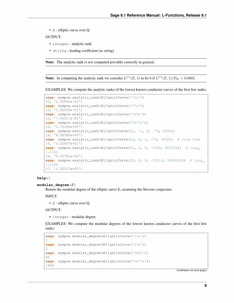
Note: The analytic rank is not computed provably correctly in general.

Note: In computing the analytic rank we consider 𝐿(𝑟)(𝐸, 1) to be 0 if 𝐿(𝑟)(𝐸, 1)/Ω𝐸 > 0.0001.

EXAMPLES: We compute the analytic ranks of the lowest known conductor curves of the first few ranks:

sage: sympow.analytic_rank(EllipticCurve('11a'))(0, '2.53842e-01')sage: sympow.analytic_rank(EllipticCurve('37a'))(1, '3.06000e-01')sage: sympow.analytic_rank(EllipticCurve('389a'))(2, '7.59317e-01')sage: sympow.analytic_rank(EllipticCurve('5077a'))(3, '1.73185e+00')sage: sympow.analytic_rank(EllipticCurve([1, -1, 0, -79, 289]))(4, '8.94385e+00')sage: sympow.analytic_rank(EllipticCurve([0, 0, 1, -79, 342])) # long time(5, '3.02857e+01')sage: sympow.analytic_rank(EllipticCurve([1, 1, 0, -2582, 48720])) # long→˓time(6, '3.20781e+02')sage: sympow.analytic_rank(EllipticCurve([0, 0, 0, -10012, 346900])) # long→˓time(7, '1.32517e+03')

help()

modular_degree(E)Return the modular degree of the elliptic curve E, assuming the Stevens conjecture.

INPUT:

• E - elliptic curve over Q

OUTPUT:

• integer - modular degree

EXAMPLES: We compute the modular degrees of the lowest known conductor curves of the first fewranks:

sage: sympow.modular_degree(EllipticCurve('11a'))1sage: sympow.modular_degree(EllipticCurve('37a'))2sage: sympow.modular_degree(EllipticCurve('389a'))40sage: sympow.modular_degree(EllipticCurve('5077a'))1984

(continues on next page)

9


(continued from previous page)

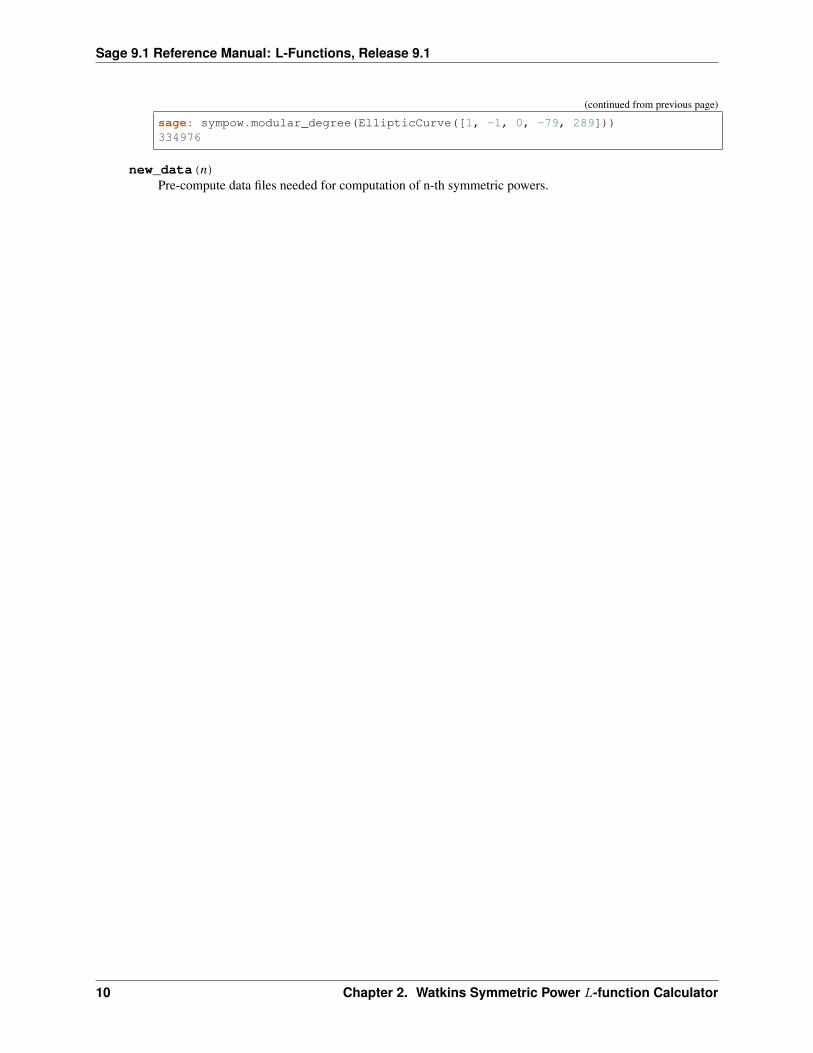
sage: sympow.modular_degree(EllipticCurve([1, -1, 0, -79, 289]))334976

new_data(n)Pre-compute data files needed for computation of n-th symmetric powers.

10 Chapter 2. Watkins Symmetric Power 𝐿-function Calculator

CHAPTER

THREE

DOKCHITSER’S L-FUNCTIONS CALCULATOR

AUTHORS:

• Tim Dokchitser (2002): original PARI code and algorithm (and the documentation below is based on Dok-chitser’s docs).

• William Stein (2006-03-08): Sage interface

Todo:

• add more examples from SAGE_EXTCODE/pari/dokchitser that illustrate use with Eisenstein series, numberfields, etc.

• plug this code into number fields and modular forms code (elliptic curves are done).

class sage.lfunctions.dokchitser.Dokchitser(conductor, gammaV, weight, eps, poles=[],residues=’automatic’, prec=53, init=None)

Bases: sage.structure.sage_object.SageObject

Dokchitser’s 𝐿-functions Calculator

Create a Dokchitser 𝐿-series with

Dokchitser(conductor, gammaV, weight, eps, poles, residues, init, prec)

where

• conductor – integer, the conductor

• gammaV – list of Gamma-factor parameters, e.g. [0] for Riemann zeta, [0,1] for ell.curves, (see examples).

• weight – positive real number, usually an integer e.g. 1 for Riemann zeta, 2 for 𝐻1 of curves/Q

• eps – complex number; sign in functional equation

• poles – (default: []) list of points where 𝐿*(𝑠) has (simple) poles; only poles with 𝑅𝑒(𝑠) > 𝑤𝑒𝑖𝑔ℎ𝑡/2should be included

• residues – vector of residues of 𝐿*(𝑠) in those poles or set residues=’automatic’ (default value)

• prec – integer (default: 53) number of bits of precision

RIEMANN ZETA FUNCTION:

We compute with the Riemann Zeta function.

sage: L = Dokchitser(conductor=1, gammaV=[0], weight=1, eps=1, poles=[1],→˓residues=[-1], init='1')sage: L


11




Dokchitser L-series of conductor 1 and weight 1sage: L(1)Traceback (most recent call last):...ArithmeticErrorsage: L(2)1.64493406684823sage: L(2, 1.1)1.64493406684823sage: L.derivative(2)-0.937548254315844sage: h = RR('0.0000000000001')sage: (zeta(2+h) - zeta(2.))/h-0.937028232783632sage: L.taylor_series(2, k=5)1.64493406684823 - 0.937548254315844*z + 0.994640117149451*z^2 - 1.→˓00002430047384*z^3 + 1.00006193307...*z^4 + O(z^5)

RANK 1 ELLIPTIC CURVE:

We compute with the 𝐿-series of a rank 1 curve.

sage: E = EllipticCurve('37a')sage: L = E.lseries().dokchitser(algorithm='gp'); LDokchitser L-function associated to Elliptic Curve defined by y^2 + y = x^3 - x→˓over Rational Fieldsage: L(1)0.000000000000000sage: L.derivative(1)0.305999773834052sage: L.derivative(1,2)0.373095594536324sage: L.num_coeffs()48sage: L.taylor_series(1,4)0.000000000000000 + 0.305999773834052*z + 0.186547797268162*z^2 - 0.→˓136791463097188*z^3 + O(z^4)sage: L.check_functional_equation()6.11218974700000e-18 # 32-bit6.04442711160669e-18 # 64-bit

RANK 2 ELLIPTIC CURVE:

We compute the leading coefficient and Taylor expansion of the 𝐿-series of a rank 2 elliptic curve.

sage: E = EllipticCurve('389a')sage: L = E.lseries().dokchitser(algorithm='gp')sage: L.num_coeffs()156sage: L.derivative(1,E.rank())1.51863300057685sage: L.taylor_series(1,4)-1.27685190980159e-23 + (7.23588070754027e-24)*z + 0.759316500288427*z^2 - 0.→˓430302337583362*z^3 + O(z^4) # 32-bit-2.72911738151096e-23 + (1.54658247036311e-23)*z + 0.759316500288427*z^2 - 0.→˓430302337583362*z^3 + O(z^4) # 64-bit

NUMBER FIELD:

12 Chapter 3. Dokchitser’s L-functions Calculator


We compute with the Dedekind zeta function of a number field.

sage: x = var('x')sage: K = NumberField(x**4 - x**2 - 1,'a')sage: L = K.zeta_function(algorithm='gp')sage: L.conductor400sage: L.num_coeffs()264sage: L(2)1.10398438736918sage: L.taylor_series(2,3)1.10398438736918 - 0.215822638498759*z + 0.279836437522536*z^2 + O(z^3)

RAMANUJAN DELTA L-FUNCTION:

The coefficients are given by Ramanujan’s tau function:

sage: L = Dokchitser(conductor=1, gammaV=[0,1], weight=12, eps=1)sage: pari_precode = 'tau(n)=(5*sigma(n,3)+7*sigma(n,5))*n/12 - 35*sum(k=1,n-1,→˓(6*k-4*(n-k))*sigma(k,3)*sigma(n-k,5))'sage: L.init_coeffs('tau(k)', pari_precode=pari_precode)

We redefine the default bound on the coefficients: Deligne’s estimate on tau(n) is better than the default coef-grow(n)=‘(4n)^11/2‘ (by a factor 1024), so re-defining coefgrow() improves efficiency (slightly faster).

sage: L.num_coeffs()12sage: L.set_coeff_growth('2*n^(11/2)')sage: L.num_coeffs()11

Now we’re ready to evaluate, etc.

sage: L(1)0.0374412812685155sage: L(1, 1.1)0.0374412812685155sage: L.taylor_series(1,3)0.0374412812685155 + 0.0709221123619322*z + 0.0380744761270520*z^2 + O(z^3)

check_functional_equation(T=1.2)Verifies how well numerically the functional equation is satisfied, and also determines the residues ifself.poles != [] and residues=’automatic’.

More specifically: for 𝑇 > 1 (default 1.2), self.check_functional_equation(T) should ide-ally return 0 (to the current precision).

• if what this function returns does not look like 0 at all, probably the functional equation is wrong (i.e.some of the parameters gammaV, conductor etc., or the coefficients are wrong),

• if checkfeq(T) is to be used, more coefficients have to be generated (approximately T times more),e.g. call cflength(1.3), initLdata(“a(k)”,1.3), checkfeq(1.3)

• T=1 always (!) returns 0, so T has to be away from 1

• default value 𝑇 = 1.2 seems to give a reasonable balance

• if you don’t have to verify the functional equation or the L-values, call num_coeffs(1) and initL-data(“a(k)”,1), you need slightly less coefficients.

13


EXAMPLES:

sage: L = Dokchitser(conductor=1, gammaV=[0], weight=1, eps=1, poles=[1],→˓residues=[-1], init='1')sage: L.check_functional_equation()-1.35525271600000e-20 # 32-bit-2.71050543121376e-20 # 64-bit

If we choose the sign in functional equation for the 𝜁 function incorrectly, the functional equation doesn’tcheck out.

sage: L = Dokchitser(conductor=1, gammaV=[0], weight=1, eps=-11, poles=[1],→˓residues=[-1], init='1')sage: L.check_functional_equation()-9.73967861488124

derivative(s, k=1)Return the 𝑘-th derivative of the 𝐿-series at 𝑠.

Warning: If 𝑘 is greater than the order of vanishing of 𝐿 at 𝑠 you may get nonsense.

EXAMPLES:

sage: E = EllipticCurve('389a')sage: L = E.lseries().dokchitser(algorithm='gp')sage: L.derivative(1,E.rank())1.51863300057685

gp()Return the gp interpreter that is used to implement this Dokchitser L-function.

EXAMPLES:

sage: E = EllipticCurve('11a')sage: L = E.lseries().dokchitser(algorithm='gp')sage: L(2)0.546048036215014sage: L.gp()PARI/GP interpreter

init_coeffs(v, cutoff=1, w=None, pari_precode=”, max_imaginary_part=0,max_asymp_coeffs=40)

Set the coefficients 𝑎𝑛 of the 𝐿-series.

If 𝐿(𝑠) is not equal to its dual, pass the coefficients of the dual as the second optional argument.

INPUT:

• v – list of complex numbers or string (pari function of k)

• cutoff – real number = 1 (default: 1)

• w – list of complex numbers or string (pari function of k)

• pari_precode – some code to execute in pari before calling initLdata

• max_imaginary_part – (default: 0): redefine if you want to compute L(s) for s having largeimaginary part,



• max_asymp_coeffs – (default: 40): at most this many terms are generated in asymptotic seriesfor phi(t) and G(s,t).

EXAMPLES:

sage: L = Dokchitser(conductor=1, gammaV=[0,1], weight=12, eps=1)sage: pari_precode = 'tau(n)=(5*sigma(n,3)+7*sigma(n,5))*n/12 - 35*sum(k=1,n-→˓1,(6*k-4*(n-k))*sigma(k,3)*sigma(n-k,5))'sage: L.init_coeffs('tau(k)', pari_precode=pari_precode)

Evaluate the resulting L-function at a point, and compare with the answer that one gets “by definition” (ofL-function attached to a modular form):

sage: L(14)0.998583063162746sage: a = delta_qexp(1000)sage: sum(a[n]/float(n)^14 for n in range(1,1000))0.9985830631627459

Illustrate that one can give a list of complex numbers for v (see trac ticket #10937):

sage: L2 = Dokchitser(conductor=1, gammaV=[0,1], weight=12, eps=1)sage: L2.init_coeffs(list(delta_qexp(1000))[1:])sage: L2(14)0.998583063162746

num_coeffs(T=1)Return number of coefficients 𝑎𝑛 that are needed in order to perform most relevant 𝐿-function computa-tions to the desired precision.

EXAMPLES:

sage: E = EllipticCurve('11a')sage: L = E.lseries().dokchitser(algorithm='gp')sage: L.num_coeffs()26sage: E = EllipticCurve('5077a')sage: L = E.lseries().dokchitser(algorithm='gp')sage: L.num_coeffs()568sage: L = Dokchitser(conductor=1, gammaV=[0], weight=1, eps=1, poles=[1],→˓residues=[-1], init='1')sage: L.num_coeffs()4

Verify that num_coeffs works with non-real spectral parameters, e.g. for the L-function of the level 10Maass form with eigenvalue 2.7341055592527126:

sage: ev = 2.7341055592527126sage: L = Dokchitser(conductor=10, gammaV=[ev*i, -ev*i],weight=2,eps=1)sage: L.num_coeffs()26

set_coeff_growth(coefgrow)You might have to redefine the coefficient growth function if the 𝑎𝑛 of the 𝐿-series are not given by thefollowing PARI function:

15

https://trac.sagemath.org/10937


coefgrow(n) = if(length(Lpoles),1.5*n^(vecmax(real(Lpoles))-1),sqrt(4*n)^(weight-1));

INPUT:

• coefgrow – string that evaluates to a PARI function of n that defines a coefgrow function.

EXAMPLES:

sage: L = Dokchitser(conductor=1, gammaV=[0,1], weight=12, eps=1)sage: pari_precode = 'tau(n)=(5*sigma(n,3)+7*sigma(n,5))*n/12 - 35*sum(k=1,n-→˓1,(6*k-4*(n-k))*sigma(k,3)*sigma(n-k,5))'sage: L.init_coeffs('tau(k)', pari_precode=pari_precode)sage: L.set_coeff_growth('2*n^(11/2)')sage: L(1)0.0374412812685155

taylor_series(a=0, k=6, var=’z’)Return the first 𝑘 terms of the Taylor series expansion of the 𝐿-series about 𝑎.

This is returned as a series in var, where you should view var as equal to 𝑠 − 𝑎. Thus this functionreturns the formal power series whose coefficients are 𝐿(𝑛)(𝑎)/𝑛!.

INPUT:

• a – complex number (default: 0); point about which to expand

• k – integer (default: 6), series is 𝑂(

• var – string (default: ‘z’), variable of power series

EXAMPLES:

sage: L = Dokchitser(conductor=1, gammaV=[0], weight=1, eps=1, poles=[1],→˓residues=[-1], init='1')sage: L.taylor_series(2, 3)1.64493406684823 - 0.937548254315844*z + 0.994640117149451*z^2 + O(z^3)sage: E = EllipticCurve('37a')sage: L = E.lseries().dokchitser(algorithm='gp')sage: L.taylor_series(1)0.000000000000000 + 0.305999773834052*z + 0.186547797268162*z^2 - 0.→˓136791463097188*z^3 + 0.0161066468496401*z^4 + 0.0185955175398802*z^5 + O(z^→˓6)

We compute a Taylor series where each coefficient is to high precision.

sage: E = EllipticCurve('389a')sage: L = E.lseries().dokchitser(200, algorithm='gp')sage: L.taylor_series(1,3)...e-82 + (...e-82)*z + 0.→˓75931650028842677023019260789472201907809751649492435158581*z^2 + O(z^3)

Check that trac ticket #25402 is fixed:

sage: L = EllipticCurve("24a1").modular_form().lseries()sage: L.taylor_series(-1, 3)0.000000000000000 - 0.702565506265199*z + 0.638929001045535*z^2 + O(z^3)

Check that trac ticket #25965 is fixed:





sage: L2 = EllipticCurve("37a1").modular_form().lseries(); L2L-series associated to the cusp form q - 2*q^2 - 3*q^3 + 2*q^4 - 2*q^5 + O(q^→˓6)sage: L2.taylor_series(0,4)0.000000000000000 - 0.357620466127498*z + 0.273373112603865*z^2 + 0.→˓303362857047671*z^3 + O(z^4)sage: L2.taylor_series(0,1)O(z^1)sage: L2(0)0.000000000000000

sage.lfunctions.dokchitser.reduce_load_dokchitser(D)

17

CHAPTER

FOUR

CLASS FILE FOR COMPUTING SUMS OVER ZEROS OF MOTIVICL-FUNCTIONS.

All computations are done to double precision.

AUTHORS:

• Simon Spicer (2014-10): first version

sage.lfunctions.zero_sums.LFunctionZeroSum(X, *args, **kwds)Constructor for the LFunctionZeroSum class.

INPUT:

• X – A motivic object. Currently only implemented for X = an elliptic curve over the rational numbers.

OUTPUT:

An LFunctionZeroSum object.

EXAMPLES:

sage: E = EllipticCurve("389a")sage: Z = LFunctionZeroSum(E); ZZero sum estimator for L-function attached to Elliptic Curve defined by y^2 + y =→˓x^3 + x^2 - 2*x over Rational Field

class sage.lfunctions.zero_sums.LFunctionZeroSum_EllipticCurveBases: sage.lfunctions.zero_sums.LFunctionZeroSum_abstract

Subclass for computing certain sums over zeros of an elliptic curve L-function without having to determine thezeros themselves.

analytic_rank_upper_bound(max_Delta=None, adaptive=True, root_number=’compute’,bad_primes=None, ncpus=None)

Return an upper bound for the analytic rank of the L-function 𝐿𝐸(𝑠) attached to self, conditional onthe Generalized Riemann Hypothesis, via computing the zero sum

∑𝛾 𝑓(∆𝛾), where 𝛾 ranges over the

imaginary parts of the zeros of 𝐿(𝐸, 𝑠) along the critical strip, 𝑓(𝑥) =(

sin(𝜋𝑥)𝜋𝑥

)2

, and ∆ is the tightnessparameter whose maximum value is specified by max_Delta. This computation can be run on curves withvery large conductor (so long as the conductor is known or quickly computable) when Delta is not toolarge (see below).

Uses Bober’s rank bounding method as described in [Bob2013].

INPUT:

• max_Delta – (default: None) If not None, a positive real value specifying the maximum Deltavalue used in the zero sum; larger values of Delta yield better bounds - but runtime is exponential inDelta. If left as None, Delta is set to min

1𝜋 (log(𝑁 + 1000)/2 − log(2𝜋) − 𝜂) , 2.5

, where 𝑁 is

19


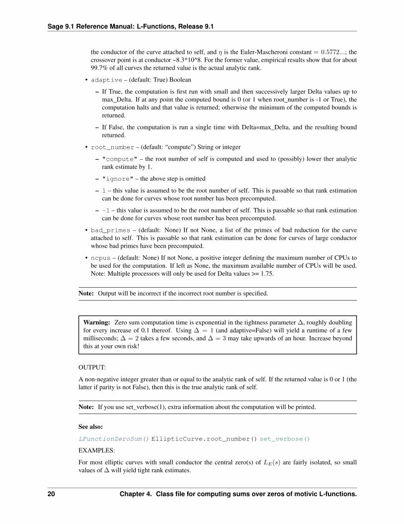
the conductor of the curve attached to self, and 𝜂 is the Euler-Mascheroni constant = 0.5772...; thecrossover point is at conductor ~8.3*10^8. For the former value, empirical results show that for about99.7% of all curves the returned value is the actual analytic rank.

• adaptive – (default: True) Boolean

– If True, the computation is first run with small and then successively larger Delta values up tomax_Delta. If at any point the computed bound is 0 (or 1 when root_number is -1 or True), thecomputation halts and that value is returned; otherwise the minimum of the computed bounds isreturned.

– If False, the computation is run a single time with Delta=max_Delta, and the resulting boundreturned.

• root_number – (default: “compute”) String or integer

– "compute" – the root number of self is computed and used to (possibly) lower ther analyticrank estimate by 1.

– "ignore" – the above step is omitted

– 1 – this value is assumed to be the root number of self. This is passable so that rank estimationcan be done for curves whose root number has been precomputed.

– -1 – this value is assumed to be the root number of self. This is passable so that rank estimationcan be done for curves whose root number has been precomputed.

• bad_primes – (default: None) If not None, a list of the primes of bad reduction for the curveattached to self. This is passable so that rank estimation can be done for curves of large conductorwhose bad primes have been precomputed.

• ncpus – (default: None) If not None, a positive integer defining the maximum number of CPUs tobe used for the computation. If left as None, the maximum available number of CPUs will be used.Note: Multiple processors will only be used for Delta values >= 1.75.

Note: Output will be incorrect if the incorrect root number is specified.

Warning: Zero sum computation time is exponential in the tightness parameter ∆, roughly doublingfor every increase of 0.1 thereof. Using ∆ = 1 (and adaptive=False) will yield a runtime of a fewmilliseconds; ∆ = 2 takes a few seconds, and ∆ = 3 may take upwards of an hour. Increase beyondthis at your own risk!

OUTPUT:

A non-negative integer greater than or equal to the analytic rank of self. If the returned value is 0 or 1 (thelatter if parity is not False), then this is the true analytic rank of self.

Note: If you use set_verbose(1), extra information about the computation will be printed.

See also:

LFunctionZeroSum() EllipticCurve.root_number() set_verbose()

EXAMPLES:

For most elliptic curves with small conductor the central zero(s) of 𝐿𝐸(𝑠) are fairly isolated, so smallvalues of ∆ will yield tight rank estimates.

20 Chapter 4. Class file for computing sums over zeros of motivic L-functions.

../../../../../../html/en/reference/misc/sage/misc/misc.html#sage.misc.misc.set_verbose


sage: E = EllipticCurve("11a")sage: E.rank()0sage: Z = LFunctionZeroSum(E)sage: Z.analytic_rank_upper_bound(max_Delta=1,ncpus=1)0

sage: E = EllipticCurve([-39,123])sage: E.rank()1sage: Z = LFunctionZeroSum(E)sage: Z.analytic_rank_upper_bound(max_Delta=1)1

This is especially true for elliptic curves with large rank.

sage: for r in range(9):....: E = elliptic_curves.rank(r)[0]....: print((r, E.analytic_rank_upper_bound(max_Delta=1,....: adaptive=False,root_number="ignore")))....:(0, 0)(1, 1)(2, 2)(3, 3)(4, 4)(5, 5)(6, 6)(7, 7)(8, 8)

However, some curves have 𝐿-functions with low-lying zeroes, and for these larger values of ∆ must beused to get tight estimates.

sage: E = EllipticCurve("974b1")sage: r = E.rank(); r0sage: Z = LFunctionZeroSum(E)sage: Z.analytic_rank_upper_bound(max_Delta=1,root_number="ignore")1sage: Z.analytic_rank_upper_bound(max_Delta=1.3,root_number="ignore")0

Knowing the root number of E allows us to use smaller Delta values to get tight bounds, thus speeding upruntime considerably.

sage: Z.analytic_rank_upper_bound(max_Delta=0.6,root_number="compute")0

The are a small number of curves which have pathologically low-lying zeroes. For these curves, thismethod will produce a bound that is strictly larger than the analytic rank, unless very large values ofDelta are used. The following curve (“256944c1” in the Cremona tables) is a rank 0 curve with a zero at0.0256. . . ; the smallest Delta value for which the zero sum is strictly less than 2 is ~2.815.

sage: E = EllipticCurve([0, -1, 0, -7460362000712, -7842981500851012704])sage: N,r = E.conductor(),E.analytic_rank(); N, r(256944, 0)


21



sage: E.analytic_rank_upper_bound(max_Delta=1,adaptive=False)2sage: E.analytic_rank_upper_bound(max_Delta=2,adaptive=False)2

This method is can be called on curves with large conductor.

sage: E = EllipticCurve([-2934,19238])sage: Z = LFunctionZeroSum(E)sage: Z.analytic_rank_upper_bound()1

And it can bound rank on curves with very large conductor, so long as you know beforehand/can easilycompute the conductor and primes of bad reduction less than 𝑒2𝜋Δ. The example below is of the rank 28curve discovered by Elkies that is the elliptic curve of (currently) largest known rank.

sage: a4 = -20067762415575526585033208209338542750930230312178956502sage: a6 =→˓34481611795030556467032985690390720374855944359319180361266008296291939448732243429sage: E = EllipticCurve([1,-1,1,a4,a6])sage: bad_primes = [2,3,5,7,11,13,17,19,48463]sage: N =→˓3455601108357547341532253864901605231198511505793733138900595189472144724781456635380154149870961231592352897621963802238155192936274322687070sage: Z = LFunctionZeroSum(E,N)sage: Z.analytic_rank_upper_bound(max_Delta=2.37,adaptive=False, # long time....: root_number=1,bad_primes=bad_primes,ncpus=2) # long time32

cn(n)Return the nth Dirichlet coefficient of the logarithmic derivative of the L-function attached to self, shiftedso that the critical line lies on the imaginary axis. The returned value is zero if 𝑛 is not a perfect primepower; when 𝑛 = 𝑝𝑒 for 𝑝 a prime of bad reduction it is −𝑎𝑒𝑝𝑙𝑜𝑔(𝑝)/𝑝𝑒, where 𝑎𝑝 is +1,−1 or 0 accordingto the reduction type of 𝑝; and when 𝑛 = 𝑝𝑒 for a prime 𝑝 of good reduction, the value is −(𝛼𝑒

𝑝 +𝛽𝑒𝑝) log(𝑝)/𝑝𝑒, where 𝛼𝑝 and 𝛽𝑝 are the two complex roots of the characteristic equation of Frobenius at 𝑝

on 𝐸.

INPUT:

• n – non-negative integer

OUTPUT:

A real number which (by Hasse’s Theorem) is at most 2 𝑙𝑜𝑔(𝑛)√𝑛

in magnitude.

EXAMPLES:

sage: E = EllipticCurve("11a")sage: Z = LFunctionZeroSum(E)sage: for n in range(12): print((n, Z.cn(n))) # tol 1.0e-13(0, 0.0)(1, 0.0)(2, 0.6931471805599453)(3, 0.3662040962227033)(4, 0.0)(5, -0.32188758248682003)(6, 0.0)(7, 0.555974328301518)





(8, -0.34657359027997264)(9, 0.6103401603711721)(10, 0.0)(11, -0.21799047934530644)

elliptic_curve()Return the elliptic curve associated with self.

EXAMPLES:

sage: E = EllipticCurve([23,100])sage: Z = LFunctionZeroSum(E)sage: Z.elliptic_curve()Elliptic Curve defined by y^2 = x^3 + 23*x + 100 over Rational Field

lseries()Return the 𝐿-series associated with self.

EXAMPLES:

sage: E = EllipticCurve([23,100])sage: Z = LFunctionZeroSum(E)sage: Z.lseries()Complex L-series of the Elliptic Curve defined by y^2 = x^3 + 23*x + 100 over→˓Rational Field

class sage.lfunctions.zero_sums.LFunctionZeroSum_abstractBases: sage.structure.sage_object.SageObject

Abstract class for computing certain sums over zeros of a motivic L-function without having to determine thezeros themselves.

C0(include_euler_gamma=True)Return the constant term of the logarithmic derivative of the completed 𝐿-function attached to self. Thisis equal to −𝜂 + log(𝑁)/2− log(2𝜋), where 𝜂 is the Euler-Mascheroni constant = 0.5772... and 𝑁 is thelevel of the form attached to self.

INPUT:

• include_euler_gamma – bool (default: True); if set to False, return the constant log(𝑁)/2 −log(2𝜋), i.e., do not subtract off the Euler-Mascheroni constant.

EXAMPLES:

sage: E = EllipticCurve("389a")sage: Z = LFunctionZeroSum(E)sage: Z.C0() # tol 1.0e-130.5666969404983447sage: Z.C0(include_euler_gamma=False) # tol 1.0e-131.1439126053998776

cnlist(n, python_floats=False)Return a list of Dirichlet coefficient of the logarithmic derivative of the 𝐿-function attached to self, shiftedso that the critical line lies on the imaginary axis, up to and including n. The i-th element of the return listis a[i].

INPUT:

• n – non-negative integer

23



• python_floats – bool (default: False); if True return a list of Python floats instead of Sage RealDouble Field elements.

OUTPUT:

A list of real numbers

See also:

cn()

Todo: Speed this up; make more efficient

EXAMPLES:

sage: E = EllipticCurve("11a")sage: Z = LFunctionZeroSum(E)sage: cnlist = Z.cnlist(11)sage: for n in range(12): print((n, cnlist[n])) # tol 1.0e-13(0, 0.0)(1, 0.0)(2, 0.6931471805599453)(3, 0.3662040962227033)(4, 0.0)(5, -0.32188758248682003)(6, 0.0)(7, 0.555974328301518)(8, -0.34657359027997264)(9, 0.6103401603711721)(10, 0.0)(11, -0.21799047934530644)

completed_logarithmic_derivative(s, num_terms=10000)Compute the value of the completed logarithmic derivative Λ′

Λ at the point s to low precision, where Λ =

𝑁𝑠/2(2𝜋)𝑠Γ(𝑠)𝐿(𝑠) and 𝐿 is the 𝐿-function attached to self.

Warning: This is computed naively by evaluating the Dirichlet series for 𝐿′

𝐿 ; the convergence thereofis controlled by the distance of s from the critical strip 0.5 <= ℜ(𝑠) <= 1.5. You may use thismethod to attempt to compute values inside the critical strip; however, results are then not guaranteedto be correct to any number of digits.

INPUT:

• s – Real or complex value

• num_terms – (default: 10000) the maximum number of terms summed in the Dirichlet series.

OUTPUT:

A tuple (z,err), where z is the computed value, and err is an upper bound on the truncation error in thisvalue introduced by truncating the Dirichlet sum.

Note: For the default term cap of 10000, a value accurate to all 53 bits of a double precision floating pointnumber is only guaranteed when |ℜ(𝑠− 1)| > 4.58, although in practice inputs closer to the critical stripwill still yield computed values close to the true value.



See also:

logarithmic_derivative()

EXAMPLES:

sage: E = EllipticCurve([23,100])sage: Z = LFunctionZeroSum(E)sage: Z.completed_logarithmic_derivative(3) # tol 1.0e-13(6.64372066048195, 6.584671359095225e-06)

Complex values are handled. The function is odd about s=1, so the value at 2-s should be minus the valueat s.

sage: Z.completed_logarithmic_derivative(complex(-2.2,1)) # tol 1.0e-13(-6.898080633125154 + 0.22557015394248361*I, 5.623853049808912e-11)sage: Z.completed_logarithmic_derivative(complex(4.2,-1)) # tol 1.0e-13(6.898080633125154 - 0.22557015394248361*I, 5.623853049808912e-11)

digamma(s, include_constant_term=True)Return the digamma function z(𝑠) on the complex input s, given by z(𝑠) = −𝜂+

∑∞𝑘=1

𝑠−1𝑘(𝑘+𝑠−1) , where

𝜂 is the Euler-Mascheroni constant = 0.5772156649 . . .. This function is needed in the computing thelogarithmic derivative of the 𝐿-function attached to self.

INPUT:

• s – A complex number

• include_constant_term – (default: True) boolean; if set False, only the value of the sum over𝑘 is returned without subtracting off the Euler-Mascheroni constant, i.e. the returned value is equal to∑∞

𝑘=1𝑠−1

𝑘(𝑘+𝑠−1) .

OUTPUT:

A real double precision number if the input is real and not a negative integer; Infinity if the input is anegative integer, and a complex number otherwise.

EXAMPLES:

sage: Z = LFunctionZeroSum(EllipticCurve("37a"))sage: Z.digamma(3.2) # tol 1.0e-130.9988388912865993sage: Z.digamma(3.2,include_constant_term=False) # tol 1.0e-131.576054556188132sage: Z.digamma(1+I) # tol 1.0e-130.09465032062247625 + 1.076674047468581*Isage: Z.digamma(-2)+Infinity

Evaluating the sum without the constant term at the positive integers n returns the (n-1)th harmonic number.

sage: Z.digamma(3,include_constant_term=False)1.5sage: Z.digamma(6,include_constant_term=False)2.283333333333333

level()Return the level of the form attached to self. If self was constructed from an elliptic curve, then this isequal to the conductor of 𝐸.

EXAMPLES:

25


sage: E = EllipticCurve("389a")sage: Z = LFunctionZeroSum(E)sage: Z.level()389

logarithmic_derivative(s, num_terms=10000, as_interval=False)Compute the value of the logarithmic derivative 𝐿′

𝐿 at the point s to low precision, where 𝐿 is the 𝐿-functionattached to self.

Warning: The value is computed naively by evaluating the Dirichlet series for 𝐿′

𝐿 ; convergence iscontrolled by the distance of s from the critical strip 0.5 <= ℜ(𝑠) <= 1.5. You may use this methodto attempt to compute values inside the critical strip; however, results are then not guaranteed to becorrect to any number of digits.

INPUT:

• s – Real or complex value

• num_terms – (default: 10000) the maximum number of terms summed in the Dirichlet series.

OUTPUT:

A tuple (z,err), where z is the computed value, and err is an upper bound on the truncation error in thisvalue introduced by truncating the Dirichlet sum.

Note: For the default term cap of 10000, a value accurate to all 53 bits of a double precision floating pointnumber is only guaranteed when |ℜ(𝑠− 1)| > 4.58, although in practice inputs closer to the critical stripwill still yield computed values close to the true value.

EXAMPLES:

sage: E = EllipticCurve([23,100])sage: Z = LFunctionZeroSum(E)sage: Z.logarithmic_derivative(10) # tol 1.0e-13(5.648066742632698e-05, 1.0974102859764345e-34)sage: Z.logarithmic_derivative(2.2) # tol 1.0e-13(0.5751257063594758, 0.024087912696974387)

Increasing the number of terms should see the truncation error decrease.

sage: Z.logarithmic_derivative(2.2,num_terms=50000) # long time # rel tol 1.→˓0e-14(0.5751579645060139, 0.008988775519160675)

Attempting to compute values inside the critical strip gives infinite error.

sage: Z.logarithmic_derivative(1.3) # tol 1.0e-13(5.442994413920786, +Infinity)

Complex inputs and inputs to the left of the critical strip are allowed.

sage: Z.logarithmic_derivative(complex(3,-1)) # tol 1.0e-13(0.04764548578052381 + 0.16513832809989326*I, 6.584671359095225e-06)sage: Z.logarithmic_derivative(complex(-3,-1.1)) # tol 1.0e-13(-13.908452173241546 + 2.591443099074753*I, 2.7131584736258447e-14)



The logarithmic derivative has poles at the negative integers.

sage: Z.logarithmic_derivative(-3) # tol 1.0e-13(-Infinity, 2.7131584736258447e-14)

ncpus(n=None)Set or return the number of CPUs to be used in parallel computations. If called with no input, the numberof CPUs currently set is returned; else this value is set to n. If n is 0 then the number of CPUs is set to themax available.

INPUT:

n – (default: None) If not None, a nonnegative integer

OUTPUT:

If n is not None, returns a positive integer

EXAMPLES:

sage: Z = LFunctionZeroSum(EllipticCurve("389a"))sage: Z.ncpus()1sage: Z.ncpus(2)sage: Z.ncpus()2

The following output will depend on the system that Sage is running on.

sage: Z.ncpus(0)sage: Z.ncpus() # random4

weight()Return the weight of the form attached to self. If self was constructed from an elliptic curve, then this is 2.

EXAMPLES:

sage: E = EllipticCurve("389a")sage: Z = LFunctionZeroSum(E)sage: Z.weight()2

zerosum(Delta=1, tau=0, function=’sincsquared_fast’, ncpus=None)Bound from above the analytic rank of the form attached to self by computing

∑𝛾 𝑓(∆(𝛾 − 𝜏)), where 𝛾

ranges over the imaginary parts of the zeros of 𝐿𝐸(𝑠) along the critical strip, and 𝑓(𝑥) is an appropriateeven continuous 𝐿2 function such that 𝑓(0) = 1.

If 𝜏 = 0, then as ∆ increases this sum converges from above to the analytic rank of the 𝐿-function, as𝑓(0) = 1 is counted with multiplicity 𝑟, and the other terms all go to 0 uniformly.

INPUT:

• Delta – positive real number (default: 1) parameter denoting the tightness of the zero sum.

• tau – real parameter (default: 0) denoting the offset of the sum to be computed. When 𝜏 = 0 the sumwill converge to the analytic rank of the 𝐿-function as ∆ is increased. If 𝜏 is the value of the imaginarypart of a noncentral zero, the limit will be 1 (assuming the zero is simple); otherwise, the limit will be0. Currently only implemented for the sincsquared and cauchy functions; otherwise ignored.

• function – string (default: “sincsquared_fast”) - the function 𝑓(𝑥) as described above. Currentlyimplemented options for 𝑓 are

27


– sincsquared – 𝑓(𝑥) =(

sin(𝜋𝑥)𝜋𝑥

)2

– gaussian – 𝑓(𝑥) = 𝑒−𝑥2

– sincsquared_fast – Same as “sincsquared”, but implementation optimized for elliptic curve𝐿-functions, and tau must be 0. self must be attached to an elliptic curve over Q given by its globalminimal model, otherwise the returned result will be incorrect.

– sincsquared_parallel – Same as “sincsquared_fast”, but optimized for parallel compu-tation with large (>2.0) ∆ values. self must be attached to an elliptic curve over Q given by itsglobal minimal model, otherwise the returned result will be incorrect.

– cauchy – 𝑓(𝑥) = 11+𝑥2 ; this is only computable to low precision, and only when ∆ < 2.

• ncpus - (default: None) If not None, a positive integer defining the number of CPUs to be usedfor the computation. If left as None, the maximum available number of CPUs will be used. Onlyimplemented for algorithm=”sincsquared_parallel”; ignored otherwise.

Warning: Computation time is exponential in ∆, roughly doubling for every increase of 0.1 thereof.Using ∆ = 1 will yield a computation time of a few milliseconds; ∆ = 2 takes a few seconds, and∆ = 3 takes upwards of an hour. Increase at your own risk beyond this!

OUTPUT:

A positive real number that bounds from above the number of zeros with imaginary part equal to 𝜏 . When𝜏 = 0 this is an upper bound for the 𝐿-function’s analytic rank.

See also:

analytic_rank_bound() for more documentation and examples on calling this method on ellipticcurve 𝐿-functions.

EXAMPLES:

sage: E = EllipticCurve("389a"); E.rank()2sage: Z = LFunctionZeroSum(E)sage: E.lseries().zeros(3)[0.000000000, 0.000000000, 2.87609907]sage: Z.zerosum(Delta=1,function="sincsquared_fast") # tol 1.0e-132.037500084595065sage: Z.zerosum(Delta=1,function="sincsquared_parallel") # tol 1.0e-112.037500084595065sage: Z.zerosum(Delta=1,function="sincsquared") # tol 1.0e-132.0375000845950644sage: Z.zerosum(Delta=1,tau=2.876,function="sincsquared") # tol 1.0e-131.075551295651154sage: Z.zerosum(Delta=1,tau=1.2,function="sincsquared") # tol 1.0e-130.10831555377490683sage: Z.zerosum(Delta=1,function="gaussian") # tol 1.0e-132.056890425029435


CHAPTER

FIVE

INDICES AND TABLES

• Index

• Module Index

• Search Page

29

../genindex.html

../py-modindex.html

../search.html


30 Chapter 5. Indices and Tables

PYTHON MODULE INDEX

lsage.lfunctions.dokchitser, 11sage.lfunctions.lcalc, 3sage.lfunctions.sympow, 7sage.lfunctions.zero_sums, 19

31


32 Python Module Index

INDEX

Aanalytic_rank() (sage.lfunctions.lcalc.LCalc method), 3analytic_rank() (sage.lfunctions.sympow.Sympow method), 8analytic_rank_upper_bound() (sage.lfunctions.zero_sums.LFunctionZeroSum_EllipticCurve method), 19

CC0() (sage.lfunctions.zero_sums.LFunctionZeroSum_abstract method), 23check_functional_equation() (sage.lfunctions.dokchitser.Dokchitser method), 13cn() (sage.lfunctions.zero_sums.LFunctionZeroSum_EllipticCurve method), 22cnlist() (sage.lfunctions.zero_sums.LFunctionZeroSum_abstract method), 23completed_logarithmic_derivative() (sage.lfunctions.zero_sums.LFunctionZeroSum_abstract method),

24

Dderivative() (sage.lfunctions.dokchitser.Dokchitser method), 14digamma() (sage.lfunctions.zero_sums.LFunctionZeroSum_abstract method), 25Dokchitser (class in sage.lfunctions.dokchitser), 11

Eelliptic_curve() (sage.lfunctions.zero_sums.LFunctionZeroSum_EllipticCurve method), 23

Ggp() (sage.lfunctions.dokchitser.Dokchitser method), 14

Hhelp() (sage.lfunctions.lcalc.LCalc method), 4help() (sage.lfunctions.sympow.Sympow method), 9

Iinit_coeffs() (sage.lfunctions.dokchitser.Dokchitser method), 14

LL() (sage.lfunctions.sympow.Sympow method), 7LCalc (class in sage.lfunctions.lcalc), 3Lderivs() (sage.lfunctions.sympow.Sympow method), 8level() (sage.lfunctions.zero_sums.LFunctionZeroSum_abstract method), 25LFunctionZeroSum() (in module sage.lfunctions.zero_sums), 19

33


LFunctionZeroSum_abstract (class in sage.lfunctions.zero_sums), 23LFunctionZeroSum_EllipticCurve (class in sage.lfunctions.zero_sums), 19logarithmic_derivative() (sage.lfunctions.zero_sums.LFunctionZeroSum_abstract method), 26lseries() (sage.lfunctions.zero_sums.LFunctionZeroSum_EllipticCurve method), 23

Mmodular_degree() (sage.lfunctions.sympow.Sympow method), 9

Nncpus() (sage.lfunctions.zero_sums.LFunctionZeroSum_abstract method), 27new_data() (sage.lfunctions.sympow.Sympow method), 10num_coeffs() (sage.lfunctions.dokchitser.Dokchitser method), 15

Rreduce_load_dokchitser() (in module sage.lfunctions.dokchitser), 17

Ssage.lfunctions.dokchitser (module), 11sage.lfunctions.lcalc (module), 3sage.lfunctions.sympow (module), 7sage.lfunctions.zero_sums (module), 19set_coeff_growth() (sage.lfunctions.dokchitser.Dokchitser method), 15Sympow (class in sage.lfunctions.sympow), 7

Ttaylor_series() (sage.lfunctions.dokchitser.Dokchitser method), 16twist_values() (sage.lfunctions.lcalc.LCalc method), 4twist_zeros() (sage.lfunctions.lcalc.LCalc method), 4

Vvalue() (sage.lfunctions.lcalc.LCalc method), 4values_along_line() (sage.lfunctions.lcalc.LCalc method), 5

Wweight() (sage.lfunctions.zero_sums.LFunctionZeroSum_abstract method), 27

Zzeros() (sage.lfunctions.lcalc.LCalc method), 5zeros_in_interval() (sage.lfunctions.lcalc.LCalc method), 6zerosum() (sage.lfunctions.zero_sums.LFunctionZeroSum_abstract method), 27

34 Index

sage reference manual: l-functions - sagemath...

Documents