Salience and Taxation: Theory and Evidence

Raj Chetty Adam Looney Kory KroftUC-Berkeley and NBER Federal Reserve Board UC-Berkeley

May 2008�

Abstract

This paper presents evidence that consumers under react to taxes that are not salientand characterizes the welfare consequences of tax policies when agents make such op-timization errors. The empirical evidence is based on two complementary strategies.First, we conducted an experiment at a grocery store posting tax inclusive prices for750 products subject to sales tax for a three week period. Scanner data show thatthis intervention reduced demand for the treated products by 8 percent. Second, we�nd that state-level increases in excise taxes (which are included in posted prices) re-duce alcohol consumption signi�cantly more than increases in sales taxes (which areadded at the register and are hence less salient). We develop simple, empirically im-plementable formulas for the incidence and e¢ ciency costs of taxation that accountfor salience e¤ects as well as other optimization errors. Contrary to conventional wis-dom, the formulas imply that the economic incidence of a tax depends on its statutoryincidence and that a tax can create deadweight loss even if it induces no change indemand. Our approach to welfare analysis yields robust results because it does notrequire speci�cation of a positive theory for why agents fail to optimize with respectto tax policies.

�We are very grateful to So�a Berto Villas-Boas and Reed Johnson for help in implementing the ex-periment and to Christopher Carpenter, Je¤rey Miron, and Lina Tetelbaum for sharing data on alcoholregulations. Thanks to George Akerlof, David Ahn, Alan Auerbach, Douglas Bernheim, Kitt Carpenter, Ju-dith Chevalier, Stefano DellaVigna, Amy Finkelstein, Michael Greenstone, Caroline Hoxby, Shachar Kariv,Peter Katuscak, Botond Koszegi, Erzo Luttmer, James Poterba, Matthew Rabin, Ricardo Reis, EmmanuelSaez, Jesse Shapiro, Andrei Shleifer, Dan Sichel, Uri Simonsohn, anonymous referees, and numerous semi-nar participants for helpful comments and discussions. Laurel Beck, Gregory Bruich, Matt Grandy, MattLevy, Ankur Patel, Ity Shurtz, James Sly, and Philippe Wingender provided outstanding research assistance.Funding was provided by NSF grant SES 0452605. The analysis and conclusions set forth are those of theauthors and do not indicate concurrence by other members of the research sta¤ or the Board of Governorsof the Federal Reserve. E-mail: chetty@econ.berkeley.edu, adam.looney@frb.gov, kroft@econ.berkeley.edu.

A central assumption in public economics is that agents optimize fully with respect to

tax policies. For example, Frank P. Ramsey�s (1927) seminal analysis of optimal commodity

taxation assumes that agents respond to tax changes in the same way as price changes.

Canonical results on tax incidence, e¢ ciency costs, and optimal income taxation (e.g. Arnold

C. Harberger 1964, James A. Mirrlees 1971, Anthony B. Atkinson and Joseph E. Stiglitz

1976) all rely on full optimization with respect to taxes.

Contrary to the full optimization assumption, there is accumulating evidence which sug-

gests that individuals are inattentive to some types of incentives.1 Inattention and imperfect

optimization could be particularly important in the case of taxation because tax systems are

complex and nontransparent in practice. Income tax schedules are typically highly nonlinear,

bene�t-tax linkages for social insurance programs are opaque (e.g. social security taxes and

bene�ts), and taxes on commodities are often not displayed in posted prices (sales taxes,

hotel city taxes, vehicle excise fees).

In the �rst half of this paper, we investigate empirically whether individuals optimize

fully with respect to taxes by analyzing the e¤ect of �salience�on behavioral responses to

commodity taxation. Speci�cally, we show that commodity taxes that are included in the

posted prices that consumers see when shopping (and are thus more salient) have larger

e¤ects on demand.2 In Xavier Gabaix and David I. Laibson�s (2006) terminology, our empir-

ical analysis shows that some types of taxes are �shrouded attributes.�In the second half of

the paper, we develop a simple method of characterizing the welfare consequences of taxation

when agents optimize imperfectly with respect to taxes.

We study the importance of salience empirically using two complementary strategies:

(1) an experiment in a grocery store and (2) an observational study of the e¤ect of alcohol

1Recent studies of inattentive behavior include prices vs. shipping fees (Tanjim Hossain and John Morgan2005, 2008), �nancial markets (Stefano DellaVigna and Joshua Pollet 2008), and rebates for car purchases(Meghan Busse, Jorge Silva-Risso, and Florian Zettelmeyer 2006). See DellaVigna (2007) for additionalexamples and a review of this literature.

2We use �tax salience� to refer to the visibility of the tax-inclusive price. When taxes are included inthe posted price, the total tax-inclusive price is more visible but the tax rate itself may be less clear. Thereis a longstanding theoretical literature on ��scal illusion�which discusses how the lack of visibility of taxrates may a¤ect voting behavior and the size of government (John S. Mill 1848). Unlike that literature,we de�ne salience in terms of the visibility of the tax-inclusive price because we focus on behaviors thatoptimally depend on total tax-inclusive prices rather than behaviors which depend on the tax rate itself.

1

taxes on alcohol consumption. The experiment was implemented at a supermarket over a

three-week period in early 2006. In this store, prices posted on the shelf exclude sales tax of

7.375 percent. If a product is subject to sales tax, it is added to the bill only at the register,

as in most other retail stores in the United States.3 To test if people under react to the sales

tax because it is not included in the posted price, we posted tags showing the tax inclusive

price below the original pretax price tags (shown in Exhibit 1). We posted these tags for all

products (roughly 750 total) in three taxable groups: cosmetics, hair care accessories, and

deodorants. A preliminary survey-based evaluation of the tags indicates that they succeed

in reminding consumers of actual tax inclusive prices. Without the tags, nearly all survey

respondents ignored taxes when calculating the total price of a basket of goods whereas with

the tags, the vast majority computed the total tax inclusive price correctly.

We analyze the e¤ect of posting tax inclusive prices on demand using a di¤erences-in-

di¤erences research design. Scanner data show that quantity sold and total revenue in the

treated group of products fell by about 8 percent during the intervention relative to two

�control groups��other products in the same aisle of the treatment store that were not

tagged and products in two other stores in nearby cities. The null hypothesis that posting

tax inclusive prices has no e¤ect on demand is rejected using both t-tests and nonparametric

permutation tests. To interpret the magnitude of the treatment e¤ect, we compare it with

the price elasticity of demand for these categories, which is in the range of 1 to 1.5. Since

showing the tax inclusive price reduced demand by nearly the same amount as a 7.375

percent price increase, we infer that most consumers do not normally take the sales tax into

account.

A concern with the experiment is that posting 750 new tags may have reduced demand

because of a �Hawthorne e¤ect� or a short-run violation of norms. This issue motivates

our second empirical strategy, which compares the e¤ect of price changes with tax changes

using observational data over a longer horizon. To implement this test, we focus on alcohol

consumption because alcohol is subject to two state-level taxes in the U.S.: an excise tax

3The sales tax a¤ects relative prices because it does not apply to all goods. Approximately 40 percentof expenditure is subject to sales tax in the United States. Since food is typically exempt, the fraction ofitems subject to sales tax in grocery stores is much lower.

2

that is included in the posted price and a sales tax that is added at the register (and hence

is less salient). Exploiting state-level changes in these two tax rates between 1970 and 2003

coupled with annual data on total beer consumption by state, we �nd that increases in the

excise tax reduce beer consumption by an order of magnitude more than similar increases

in the sales tax. A simple calibration shows that the magnitude of the di¤erence in the

elasticity estimates cannot be explained purely by the fact that the sales tax applies to a

broader base, especially since food and nonalcoholic beverages are exempt from sales tax

in most states. The di¤erence in elasticities persists over time, indicating that behavioral

responses to taxes and prices di¤er even in the long run.

Why do consumers under react to taxes that are not included in posted prices? One

explanation is that customers are uninformed about the sales tax rate or which goods are

subject to sales tax. An alternative hypothesis is that salience matters: the customers

know what is taxed, but focus on the posted price when shopping. To distinguish between

these hypotheses, we surveyed grocery shoppers about their knowledge of sales taxes. The

median individual correctly reported the tax status of 7 out of the 8 products on the survey,

indicating that our empirical �ndings are driven by salience e¤ects. A key feature of salience

is that it matters in steady state, and not just on the transition path after tax changes.

Motivated by this evidence, we analyze the implications of salience e¤ects and other

optimization errors for the welfare consequences of taxation. The challenge in this analysis,

as in behavioral public economics more generally, is the calculation of welfare when behavior

is inconsistent with full optimization. We characterize the e¤ect of taxes on social surplus

(excess burden) and distribution (incidence) using an approach that does not rely on a

speci�c positive model of behavior, as in B. Douglas Bernheim and Antonio Rangel (2007).

Our approach relies on two assumptions: (1) the tax a¤ects welfare only through its e¤ect

on the consumption bundle chosen by the agent and (2) consumption choices when prices

are fully salient are consistent with full optimization. Under these assumptions, we derive

approximate formulas for the incidence and e¢ ciency costs of taxation that depend only on

the empirically observed demand function and not on the underlying model which generates

that demand function. Intuitively, there are two demand curves that together are su¢ cient

statistics for welfare calculations when individuals make optimization errors: the tax-demand

3

curve, which tells us how demand varies with taxes that are not included in posted prices,

and the price-demand curve, which tells us how demand varies as (fully salient) posted prices

change. We use the tax-demand curve to determine the e¤ect of the tax on behavior and then

use the price-demand curve to calculate the e¤ect of that change in behavior on welfare. The

price-demand curve can be used to recover the agent�s underlying preferences and calculate

welfare because it is generated by optimizing behavior.

The bene�ts of this approach to welfare analysis are its simplicity and adaptability. The

formulas for excess burden and incidence can be derived using supply and demand diagrams

and familiar notions of consumer and producer surplus. The formulas di¤er from the stan-

dard Harberger (1964) expressions by a single factor � the ratio of the compensated tax

elasticity to the compensated price elasticity. Thus, one can calculate the (partial equilib-

rium) deadweight cost and incidence of any tax policy by estimating both the tax and price

elasticities instead of just the tax elasticity as in the existing empirical literature. Although

we motivate our welfare analysis by evidence of salience e¤ects, the formulas account for

all errors that consumers may make when optimizing with respect to taxes.4 For example,

confusion between average and marginal income tax rates (Charles de Bartolome (1995), Jef-

frey B. Liebman and Richard J. Zeckhauser (2004), Naomi E. Feldman and Peter Katu�µcák

(2006)) or over perception of estate tax rates (Robert J. Blendon et al. (2003), Joel B. Slem-

rod (2006)) can be handled using exactly the same formulas, without requiring knowledge

of individuals�tax perceptions and information set.

Our welfare results challenge widely held intuitions based on the full optimization model.

First, the agent who bears the statutory incidence of a tax bears more of the economic

incidence, violating the classic tax neutrality result in competitive markets. Second, a tax

increase can have a substantial e¢ ciency cost even when demand for the taxed good does

not change by distorting consumption allocations for inattentive individuals. Finally, holding

�xed the tax elasticity of demand, we show that an increase in the price elasticity of demand

reduces deadweight loss and increases incidence on consumers.

4Our formulas do not, however, permit errors in optimization relative to salient prices. Such errors can beaccommodated by isolating a condition where the true price elasticity is revealed and applying the formulashere.

4

This paper builds on and relates to several recent papers in public economics. Our theo-

retical analysis can be viewed as an application of Bernheim and Rangel�s (2007) choice-based

approach to welfare, where the choices when taxes are salient reveal an agent�s true rankings

(see section IV for more details). Our analysis also relates to the recent work of Liebman

and Zeckhauser (2004), who analyze optimal income taxation in a model where individuals

misperceive tax schedules because of �ironing� or �spotlighting� behavior. Our approach

does not require assumptions about whether individuals iron, spotlight, or respond in some

other way to the tax schedule, as any of these behaviors are captured in the empirically

observed tax and wage elasticities of labor supply.

Our empirical results are consistent with those of Amy N. Finkelstein (2007) and Tomer

Blumkin, Bradley J. Ru­ e, and Yosi Ganun (2008), who �nd evidence of salience e¤ects

in toll collection and a lab experiment on consumption vs. income taxes. One notable

study that does not �nd that salience matters is Harvey S. Rosen (1976), who shows that

the cross-sectional correlation between marginal tax rates and work hours is similar to the

correlation between wage rates and work hours. The cross-sectional approach to estimation

of wage elasticities has since been shown to su¤er from serious identi�cation problems, which

could explain why our use of credibly exogenous variation to identify salience e¤ects yields

di¤erent results.

The remainder of the paper is organized as follows. Section I presents an organizing

framework for our empirical analysis. Section II discusses the grocery experiment. Section

III presents the evidence on alcohol sales. Section IV explores why consumers under react

to taxes. Section V presents the theoretical welfare analysis. Section VI concludes.

I Empirical Framework

To motivate the empirical analysis, consider consumer behavior in an economy with two

goods, x and y, that are supplied perfectly elastically.5 Normalize the price of y to 1 and

let p denote the pretax price of x. Assume that y is untaxed and x is subject to an ad

5The supply curve is e¤ectively �at in both of our empirical strategies. In the grocery experiment,stocking patterns and prices are set at a regional level and are exogenous to our small intervention. In thealcohol analysis, we show that state-level changes in taxes on producers are shifted fully to consumers.

5

valorem sales tax �S. The total price of x is q = (1 + �S)p. The price that consumers

see when deciding what to purchase is p; the sales tax is not included in the posted price.

Since consumers must calculate q themselves but can see p directly, we will say that the tax

inclusive price q is less �salient�than the pretax price p.

Let x(p; �S) denote demand as a function of the posted price and the ad-valorem sales

tax. In the neoclassical full-optimization model, demand depends only on the total tax

inclusive price: x(p; �S) = x((1 + �S)p; 0). If consumers optimize fully, a 1 percent increase

in p and a 1 percent increase in the gross-of-tax price (1 + �S) reduce demand by the same

amount: "x;p � �@ log x@ log p

= "x;1+�S � � @ log x@ log(1+�S)

. We hypothesize that in practice consumers

under react to the tax �S because it is less salient: "x;p > "x;1+�S . To test this hypothesis,

we log-linearize the demand function x(p; �S) to obtain the following estimating equation:

log x(p; �S) = �+ � log p+ ��� log(1 + �S) (1)

In this equation, the parameter �� measures the degree to which agents under react to the

tax.6 In particular, �� is the ratio of the tax elasticity of demand ("x;1+�S = ����) to the

price elasticity of demand ("x;p = ��):

�� =@ log x

@ log(1 + �S)=@ log x

@ log p="x;1+�S

"x;p(2)

The null hypothesis of full optimization implies �� = 1. We use two empirical strategies to

estimate �� .

Strategy 1: Manipulate Tax Salience. Our �rst empirical strategy is to make the sales

tax as salient as the pretax price by posting the tax inclusive price q on the shelf. When

tax inclusive prices are posted, consumers presumably optimize relative to the tax inclusive

price and set demand to x((1 + �S)p; 0). Hence, the e¤ect of posting the tax inclusive price

6The parameter �� does not have a structural interpretation because we have not speci�ed an economicmodel that generates (1). In a companion paper (Raj Chetty, Adam Looney, and Kory Kroft 2007), wedevelop a bounded rationality model in which agents face heterogeneous cognitive costs of computing tax-inclusive prices. In that model, � is the fraction of individuals whose cognitive costs lie below the thresholdwhere it is optimal to compute the tax inclusive price.

6

on demand is

log x((1 + �S)p; 0)� log x(p; �S) = (1� �� )� log(1 + �S)

Recalling that "x;p = ��, we obtain the following estimator for �� :

(1� �� ) = �log x((1 + �S)p; 0)� log x(p; �S)

"x;p log(1 + �S). (3)

The right hand side of this equation measures the e¤ect of posting tax inclusive prices on

demand divided by the e¤ect of a price increase corresponding to the size of the tax. This

ratio measures the degree of misperception of total prices when taxes are not included in

posted prices. If all consumers normally take the sales tax into account, posting q should

have no e¤ect on demand (�� = 1), since it is redundant information. If all consumers ignore

the sales tax, posting q should reduce demand by "x;p log(1 + �S), implying �� = 0.

Strategy 2: Manipulate Tax Rate. An alternative method of estimating �� is to exploit

independent variation in �S and p to estimate the sales tax elasticity "x;1+�S and the price

elasticity "x;p, as in Rosen (1976). As shown in (2), the ratio of the two elasticities "x;1+�S="x;p

identi�es �� .

In the next section, we implement strategy 1 using a �eld experiment at a grocery store.

In section III, we implement strategy 2 using observational data on alcohol consumption.

II Evidence from an Experiment at a Grocery Store

II.A Research Design

We conducted an experiment posting tax inclusive prices at one store of a national grocery

chain. The store is a 37,000 square foot supermarket with annual revenue of approximately

$25 million and is located in a middle-income suburb in Northern California. Approximately

30 percent of the products sold in the store are subject to the local sales tax of 7.375 percent,

which is added at the register. Price tags on the shelves display only pretax prices, as in the

upper half of the tag shown in Exhibit 1.

7

The grocery chain�s managers expected that posting tax inclusive prices would reduce

sales.7 To limit revenue losses, they asked us to restrict our intervention to three product

groups that were not �sales leaders�and to limit the duration of the intervention to three

weeks. We looked for three product groups that met this requirement as well as two

additional criteria: (1) products with relatively high prices so that the dollar amount of the

sales tax is nontrivial; and (2) products belonging to �impulse purchase categories��goods

that exhibit high price elasticities �so that the demand response to the intervention would

be detectable. We chose three groups of taxable toiletries: cosmetics, hair care accessories,

and deodorants. These three product groups take up half an aisle of the store and together

include about 750 distinct products.

We posted tax inclusive prices for all products in the three groups beginning on February

22, 2006 and ending on March 15, 2006.8 Exhibit 1 shows how the price tags were altered.

The original tags, which show pretax prices, were left untouched on the shelf. A tag showing

the tax inclusive price was attached directly below this tag for each product. The added

tag stated �Total Price: $p + Sales Tax = $q,�where p denotes the pretax price (repeating

the information in the original tag) and q denotes the tax inclusive price. The original

pretax price was repeated on the new tag to avoid giving the impression that the price of the

product had increased. For the same reason, the fonts used for p, q, and the words �Sales

Tax�exactly matched the font used by the store for the original price. Additional details on

experiment implementation are given in Appendix A.

Evaluation of Tags. To determine whether the tags are e¤ective in increasing tax salience

and are understood by consumers, we conducted a preliminary survey-based evaluation in

an undergraduate class. We showed the students a photograph of taxable products on the

shelf at the grocery store similar to that in Exhibit 1. We distributed surveys (shown in

Appendix Exhibit 1) asking each student to choose two goods and write down �the total bill

7We estimate that the loss in revenue due to our experiment was about $300 (8% of $3900). Extrapolatingfrom this estimate, if taxes were included in posted prices for all taxable products, the revenue loss wouldbe 2.4 percent, or $600,000 per year per store. Note that this calculation ignores general equilibrium e¤ectsthat would arise if all retailers were required to post tax-inclusive prices.

8The treatment of showing tax inclusive price tags could have been randomized at the individual productlevel. However, the concern that such an intervention could be deceptive (e.g. suggesting that one lipstick istaxed and another is not) dissuaded us from pursuing this strategy. We therefore tagged complete productgroups, so that any direct substitute for a treated product would also be treated.

8

due at the register for these two items.� We �rst showed the photograph with the regular

tags displaying only the pretax prices. After collecting the survey responses, we showed a

second photograph of products with our tax inclusive price tags and asked students to repeat

the exercise. The results are summarized in the �rst panel of Table 1. When presented with

the �rst photo, the modal response was the total pretax bill for the two products. Only 18

percent of students reported a total price within $0.25 of the total tax inclusive amount.

When presented with the second photo, the modal response included the sales tax, and 75

percent wrote down an amount within $0.25 of the true tax inclusive total. This evidence

shows that posting tax inclusive price tags does indeed have a strong ��rst stage� e¤ect

on tax salience. Moreover, the results allay concerns that the tags confused consumers into

believing that these items were subject to an additional tax or that the pretax price of the

product had been increased.

Although we are con�dent that the tags increased tax salience substantially, we cannot

rule out the possibility that they also a¤ected demand through other channels or �Hawthorne

e¤ects.�For instance, the very fact that 750 new tags were posted on the shelves could have

deterred customers from the aisle. We are only able to estimate the e¤ect of posting the tags

on demand, and have no means of decomposing the e¤ect of the intervention into the various

mechanisms through which the tags may have had an e¤ect. The large �rst-stage e¤ect of

the tags on perceived prices leads us to believe that the primary mechanism is increased tax

salience, but we ultimately rely on evidence from the second empirical approach (see section

III) to address such concerns.

Empirical Strategy. To estimate the e¤ect of our intervention on demand, we compare

changes in quantity sold in the �treatment� group of products whose tags were modi�ed

with two �control� groups. We de�ne the treatment group as products that belong to

the cosmetics, hair care accessories, or deodorants product groups in the store where we

conducted the experiment. The �rst control group is a set of products in the same aisles

as the treatment products for which we did not change tags within the experimental store.

These products include similar (taxable) toiletries such as toothpaste, skin care, and shaving

products; see Table 2 in Appendix A for the full list. The second control group consists

of all the toiletry products sold in a pair of stores in nearby cities. These control stores

9

were selected to match the treatment store prior to the experiment on the demographic

and store characteristics shown in Table 2 in Appendix A. Using these two control groups,

we implement a standard di¤erence-in-di¤erence methodology to test whether sales of the

treated products fell during the intervention relative to the controls.

II.B Data and Summary Statistics

We use scanner data from the treatment store and the two control stores, spanning week 1

of 2005 to week 15 of 2006. The dataset contains weekly information on price and quantity

sold for all toiletry (treatment and control) products in each store. See Appendix A for

details on the dataset.

Within the treatment group, there are 13 product �categories� (e.g. lipsticks, eye cos-

metics, roll-on deodorants, body spray deodorants). The control product group contains 95

categories, which are listed in Appendix Table 1. We analyze the data at the category level

(summing quantity sold and revenue over the individual products within categories) rather

than the product level for two reasons. First, the intervention was done at the category

level. Second, we cannot distinguish products that were on the shelf but did not sell (true

zeros) from products that were not on the shelf. Analyzing the data at the category level

circumvents this problem because there are relatively few category-weeks with missing data

(4.7 percent of all observations). Since all the categories always existed in all stores through-

out the sample period, we believe that these observations are true zeros, and code them as

such.

Table 2 presents summary statistics for the treatment and control product groups in

each store. The treatment store sold an average of 25 items per category and earned $98 of

revenue per week per category over the sample period (column 1 of Table 2). The treatment

products thus account for approximately $1,300 of revenue per week as a whole. Average

weekly quantity sold per category is similar for the control products in the treatment store,

but products in these categories are somewhat more expensive on average (column 2). Sales

and revenue for the same categories in the control stores are very similar to those in the

treatment store (columns 3-4).

10

II.C Results

Comparison of Means. We begin the data analysis with a cross-tabulation of mean quantity

sold in Table 3. The upper panel of the table shows data for the treatment store. The data

is split into four cells. The rows split the data by time (pre experiment vs. the intervention

period), while the columns split the data by product group (treated vs. control categories).

Each cell shows the mean quantity sold for the group labelled on the axes, along with the

standard error and the number of observations. All standard errors reported in this and

subsequent tables in this section are clustered by week to adjust for correlation of errors

across products.9

The mean quantity sold in the treatment categories fell by an average of 1.30 units per

week during the experimental period relative to the pre period baseline. Meanwhile, quantity

sold in the control categories within the treatment store went up by 0.84 units. Hence, sales

fell in the treatment categories relative to the control categories by 2.14 units on average,

with a standard error of 0.68. This change of DDTS = �2:14 units is the �within treat-

ment store� di¤erence-in-di¤erence estimate of the impact of posting tax inclusive prices.

The identi�cation assumption necessary for consistency of DDTS is the standard �common

trends�condition (Bruce D. Meyer 1995), which in this case requires that sales of the treat-

ment and control products would have evolved similarly absent our intervention.

One natural way of evaluating the validity of this identi�cation assumption is to compare

the change in sales of treatment and control products in the control stores, where no inter-

vention took place. The lower panel of Table 3 presents such a comparison. In the control

stores, sales of treatment products increased by a (statistically insigni�cant) DDCS = 0:06

units relative to sales of control products. The fact that DDCS is not signi�cantly di¤er-

ent from zero suggests that sales of the treatment and control products would in fact have

evolved similarly in the treatment store had the intervention not taken place.

Putting together the upper and lower panels of Table 3, one can construct a �triple

di¤erence�(DDD) estimate of the e¤ect of the intervention, as in Jonathan Gruber (1994).

This estimate is DDD = DDTS �DDCS = �2:20. This estimate is statistically signi�cant

9Standard errors are similar when we cluster by category to adjust for serial correlation.

11

with p < 0:01, rejecting the null of full-optimization (�� = 1). Note that both within-

store and within-product time trends are di¤erenced out in the DDD. The DDD estimate is

therefore immune to both store-speci�c shocks �such as a transitory increase in customer

tra¢ c � and product-speci�c shocks � such as �uctuations in demand for certain goods.

Hence, the identi�cation assumption for consistency of the DDD estimate is that there was

no shock during our experimental intervention that di¤erentially a¤ected sales of only the

treatment products in the treatment store. In view of the planned, exogenous nature of the

intervention, we believe that this condition is likely to be satis�ed.

To gauge the magnitude of the estimated e¤ect, we use the framework in section I. The

mean quantity sold per category fell by 2:2 units per week, relative to a base of 29 units sold

per week. Making the sales tax salient thus reduces demand by 7.6 percent. We show below

that the estimated price elasticity of demand at the category level is "x;p = 1:59. Given

the sales tax rate of 7.375 percent, plugging these values into (3) yields a point estimate of

�� = 1 � 7:61:59�7:375 = 0:35. That is, a 10 percent tax increase reduces demand by the same

amount as a 3.5 percent price increase.

Regression Estimates. We evaluate the robustness of the DDD estimate by estimating

a series of regression models with various covariate sets and sample speci�cations in Table

4. Let the outcome of interest (e.g. quantity, log quantity, revenue) be denoted by Y . Let

the variables TS (treatment store), TC (treatment categories), and TT (treatment time)

denote indicators for whether an observation is in the experimental store, categories, and

time, respectively. Let X denote a vector of additional covariates. We estimate variants of

the following linear model, which generalizes the DDD method above (see Gruber 1994):

Y = �+ �1TT + �2TS + �3TC + 1TT � TC + 2TT � TS + 3TS � TC

+�TT � TC � TS + �X + " (4)

In this speci�cation, the third-level interaction (�) captures the treatment e¤ect of the ex-

periment and equals the DDD estimate when no additional covariates are included.

Speci�cation 1 of Table 4 estimates (4) for quantity sold, controlling for the mean price of

the products in each category using a quadratic speci�cation and including category, week,

12

and store �xed e¤ects.10 The estimated e¤ect of the treatment is essentially the same as in

the comparison of means, which is not surprising since there were no unusual price changes

during our intervention period. Speci�cation 2 shows that the intervention led to a signi�cant

reduction in revenue (price�quantity) from the treated products.11

In speci�cation 3, we estimate an analogous model in logs instead of levels. In this

speci�cation, we weight each observation by the mean revenue over time by category by

store, placing greater weight on the larger categories as in the levels regressions. The

log speci�cation is perhaps a better model for comparisons across categories with di¤erent

baseline quantities, but it forces us to omit observations that have zero quantity sold. It

yields a slightly larger estimate than the levels model for the reduction in quantity sold (10.1

percent). The estimated category-level price elasticity �the e¤ect of a 1 percent increase

in the prices of all goods within a category �is "x;p = 1:59. This elasticity is identi�ed by

the variation in average category-level prices across weeks within the stores. The estimate

is consistent with those of Stephen J. Hoch et al. (1995), who estimate a full product-level

demand system and obtain category-level price elasticities of 1 to 1.5 for similar products

using scanner data from the same grocery chain.

Placebo and Permutation Tests. To further evaluate the �common trends�identi�cation

assumption, we check for unusual patterns in demand immediately before and after the

experiment. We replicate speci�cation 1 including indicator variables for the three week

periods before the intervention began (BT ) and after the intervention ended (AT ). We also

include second- and third-level interactions of BT and AT with the TC and TS variables,

as for the TT variable in (4). Column 4 of Table 4 reports estimates of the third-level

interactions for the periods before, during, and after the experiment. Consistent with the

10The mean price is de�ned as the average price of the products in each category in the relevant week,weighted by quantity sold over the sample period. The �xed weights eliminate any mechanical relationshipbetween �uctuations in quantity sold and the average price variable.11Studies in the marketing literature (e.g., Eric T. Anderson and Duncan I. Simester 2003) �nd that

demand drops discontinuously when prices cross integer thresholds (such as $3.99 vs. $4.01), and thatretailers respond by setting prices that end in �9�to maximize pro�ts. Indeed, the retailer we study sets mostproducts�pretax prices just below the integer threshold �an observation that in itself supports our claim thatindividuals focus on the pretax price, since the tax inclusive price is often above the integer threshold. We�nd no evidence that demand fell more for the products whose price crossed the integer threshold once taxeswere included (e.g. $3.99 + Sales Tax = $4.28), but the di¤erence in the treatment e¤ects is impreciselyestimated.

13

other results in Table 4, quantity sold in the treatment group is estimated to change by

� = �2:27 units during the intervention. The corresponding �placebo� estimates for the

periods before and after the treatment are close to zero, indicating that the fall in demand

coincides precisely with the intervention period.

A concern in DD analysis is that serial correlation can bias standard errors, leading

to overrejection of the null hypothesis of no e¤ect (Marianne Bertrand, Esther Du�o, and

Sendhil Mullainathan 2002). To address this concern, we implement a nonparametric per-

mutation test for � = 0. We �rst choose a �placebo triplet�consisting of a store, three week

time period, and a randomly selected set of 13 product categories. We then estimate (4),

pretending that the placebo triplet is the treatment triplet. We repeat this procedure for all

permutations of stores and contiguous three week periods and 25 di¤erent randomly selected

groups of 13 categories, obtaining 63 � 3 � 25 = 4; 725 placebo estimates. De�ning G(b�P )to be the empirical cdf of these placebo e¤ects, the statistic G(�) gives a p-value for the

hypothesis that � = 0. Intuitively, if the experiment had a signi�cant e¤ect on demand, we

would expect the estimated coe¢ cient to be in the lower tail of estimated placebo e¤ects.12

Since this test does not make parametric assumptions about the error structure, it does not

su¤er from the overrejection bias of the t-test.

Figure 1 illustrates the results of the permutation test by plotting the empirical distribu-

tion of placebo e¤ects G for log quantity (speci�cation 3 of Table 4). The vertical line in the

�gure denotes the treatment e¤ect reported in Table 4. For log quantity, G(�) = 0:07. An

analogous test for log revenue yields G(�) = 0:04. Although these p-values are larger than

those obtained using the t-tests, they con�rm that the intervention led to an unusually low

level of demand.

Finally, we consider subsets of the large set of counterfactuals across time, categories, and

stores. In column 5 of Table 4, we restrict the sample to the treatment product categories

and compare across time and stores. This DD estimate is quite similar to the DDD estimates.

Results are also similar when we restrict the sample to the treatment store or limit the pre

experiment sample to the three months immediately before the intervention.

12This test is an extension of Ronald A. Fisher�s (1922) �exact test�for an association between two binaryvariables. See Paul R. Rosenbaum (1996) for more on permutation tests.

14

III Evidence fromObservational Data on Alcohol Sales

III.A Research Design

We turn now to the second empirical test: comparing the e¤ect of increases in posted prices

and taxes on demand. We implement this strategy by focusing on alcohol consumption.

Alcohol is subject to two taxes in most states: (1) an excise tax that is levied at the

wholesale level and is included in the price posted on the shelf or restaurant menu and (2)

a sales tax, which is added at the register (except in Hawaii, which we exclude). The total

price of alcohol is therefore q = p(1+�E)(1+�S) where p is the pretax price, �E is the excise

tax, and �S is the sales tax. Since the excise tax is included in the posted price, it is more

salient than the sales tax.

We estimate the e¤ect of �E and �S on alcohol consumption by exploiting the many

state-level changes in the two taxes between 1970 and 2003. Our estimating equation is

based on the demand speci�cation in (1):

log x = �+ � log(1 + �E) + ��� log(1 + �S). (5)

We estimate (5) in �rst-di¤erences because both the tax rates and alcohol consumption are

highly autocorrelated series. Letting t index time (years) and j index states, de�ne the

di¤erence operator �zjt = zjt�zj;t�1. Introducing a set of other demand-shifters Xjt and an

error term "jt to capture idiosyncratic state-speci�c demand shocks, we obtain the following

estimating equation by �rst-di¤erencing (5):

� log bxjt = �0 + �� log(1 + �Ejt) + ���� log(1 + �Sjt) +Xjt�+ "jt (6)

We estimate variants of (6) using OLS and test the hypothesis that �� = 1.13 The iden-

ti�cation assumption is that the changes in sales and excise taxes are uncorrelated with

state-speci�c shocks to alcohol consumption.

13The full-optimization model predicts �� = 1 irrespective of the incidence of the taxes. If tax increasesare passed through fully to the consumer �which appears to be the case in practice as we show below ��equals the price elasticity of demand.

15

III.B Data and Summary Statistics

Tax rates on alcohol vary across beer, wine, and spirits. In the interest of space, we present

results for beer, which accounts for the largest share of alcohol consumption in the U.S. A

parallel analysis using data on wine taxes and consumption for a smaller subset of years

yields similar results. We use data on aggregate annual beer consumption by state from

the National Institute of Alcohol Abuse and Alcoholism (NIAAA) (2006) from 1970-2003.

These data are compiled from administrative state tax records, and are more precise than

data from surveys because they re�ect total consumption in each state.

We obtain data on beer excise tax and sales tax rates and revenues by state from the

Brewer�s Almanac (various years), World Tax Database (2006), and other sources.14 The

state sales tax is an ad valorem tax (proportional to price), while the excise tax is typically a

speci�c tax (dollars per gallon of beer). We convert the excise tax rate into percentage units

comparable to the sales tax by dividing the beer excise tax per case in year 2000 dollars by

the average cost of a case of beer in the United States in the year 2000.15 We normalize the

excise tax by the average national price because each state�s price is endogenous to its tax

rate. Details on the data sources and construction of tax rates are given in Appendix A.

Table 5 shows summary statistics for the pooled dataset. Between 1970 and 2003, mean

per capita consumption of beer is roughly 240 cans per year. The average state excise tax

rate is 6.4 percent of the average price, while the mean state sales tax rate is 4.3 percent.16

There is considerable independent variation within states in the two taxes over the sample

period. There are 153 legislated changes to the sales tax and 131 legislated changes to excise

taxes; the correlation between excise tax changes and sales tax changes is 0.06.

14We exclude West Virginia (WV) because of problems with the sales tax rate data described in AppendixA. Including WV magni�es the di¤erence between the excise and sales tax elasticities.15Real growth in the price of beer could lead to mismeasurement of beer prices and excise tax rates

early in the sample. Using a subset of the data for which we have information on beer prices from theAmerican Chamber of Commerce Researchers Association (ACRRA) cost-of-living survey, we �nd that beerprice growth closely tracks changes in the CPI. Moreover, we show below that instrumenting for the actualACCRA price in each state/year for which it is available using our construction of the excise tax rate yieldssimilar results.16Some cities also levy local sales taxes on top of the state sales tax. In Chetty, Looney, and Kroft (2007),

we show that including local sales taxes by imputing them from data on local tax revenues does not a¤ectthe results.

16

III.C Results

We begin with a graphical analysis to illustrate the relationship between alcohol consumption

and taxes in Figures 2a and 2b. These �gures plot annual state-level changes in log beer

consumption per capita against log changes in the gross-of-excise-tax price � log(1+�E) and

the gross-of-sales-tax price � log(1 + �S). To construct Figure 2a, we �rst round each state

excise tax change to the nearest tenth of a percent. We then compute the mean change in

log beer consumption for observations with the same rounded excise tax change. Finally, we

plot the mean consumption change against the rounded excise tax rates, superimposing a

best-�t line on the points as a visual aid. Figure 2b is constructed analogously using sales tax

changes. To make the range of changes in the excise tax comparable to the smaller range of

changes in the sales tax, we restrict the range of both tax changes to �:02 log points. Figure

2a shows that increases in the beer excise tax sharply reduce beer consumption. Figure 2b

shows that increases in the sales tax have a much smaller e¤ect on beer consumption.

Regression Estimates. Table 6 presents estimates of the model for the state-level growth

rate of alcohol consumption in (6). In these and all subsequent speci�cations, we adjust

for potential serial correlation in errors by clustering the standard errors by state. Column

1 reports estimates of a baseline model that includes only year �xed e¤ects (which remove

aggregate trends) and log state population growth as covariates. In this speci�cation, a 1

percent increase in the gross-of-excise-tax price is estimated to reduce beer consumption by

0.87 percent ("x;1+�E = 0:87).17 In contrast, a 1 percent increase in the gross-of-sales-tax

price is estimated to reduce beer consumption by 0.20 percent ("x;1+�S = 0:20). The null

hypothesis that the excise and sales tax elasticities are equal is rejected with p = 0:05.

Columns 2-4 control for factors that may be correlated with the tax changes. One concern

is that sales tax changes are correlated with the business cycle. In column 2, we control for

the state-level business cycle by including changes in log state per capita income and the

state unemployment rate as covariates. Introducing these controls reduces the estimated

sales tax coe¢ cient, and as a result the null hypothesis of equal elasticities is rejected with

17This elasticity estimate is consistent with estimates of the elasticity of beer consumption with respectto the excise tax rate ("x;�E ) reported in previous studies. For example, Philip J. Cook, Jan Ostermann,and Frank A. Sloan (2005) estimate that a $0.01 increase in the beer tax per ounce of ethanol reduces beerconsumption by 1.9 percent, which translates to "x;1+�E = 1:26 at the sample mean.

17

p = 0:01. The sales tax e¤ect is smaller because sales taxes are sometimes raised during

budgetary shortfalls that occur in recessions. Since alcohol is a normal good (as indicated

by the coe¢ cients on per capita income and unemployment rate), failing to control for the

business cycle biases the correlation between alcohol consumption and sales tax changes

upward in magnitude. Hence, the endogeneity of sales tax rate appears to work against

rejecting the null hypothesis that "x;1+�E = "x;1+�S .18

Another concern is that excise tax increases are sometimes associated with contempora-

neous tightening of alcohol regulations. We evaluate this concern using data on four regu-

lations: the legal drinking age, the blood alcohol content limit, implementation of stricter

drunk driving regulations for youths, and introduction of administrative license revocation

laws. We control for the change in the legal drinking age (in years) and separate indicator

variables for a shift toward stricter regulations in each of the other three measures in column

3. The coe¢ cient on the excise tax rate does not change signi�cantly because regulation

changes have modest e¤ects on total beer consumption; on average, beer consumption falls

by only 0.5 percent when one of the four regulations is tightened.

A third concern is that trends in excise tax rates may be correlated with changes in

social norms, which directly in�uence alcohol consumption. For example, rising acceptance

of alcohol consumption in historically conservative regions such as the South may have led

to both a reduction in the excise tax as a percentage of price and an increase in alcohol

consumption. To assess whether such trends lead to signi�cant bias, we include region

�xed e¤ects in column 4 of Table 6, e¤ectively identifying the model from changes in taxes

in geographically adjacent states. The coe¢ cient on the excise rate remains substantially

larger than the coe¢ cient on the sales tax, suggesting that our results are not spuriously

generated by region-speci�c trends.

There are two sources of variation identifying the excise tax coe¢ cient: (1) policy changes

in the nominal tax rate, which produce sharp jumps in tax rates and (2) gradual erosion

of the nominal value of the tax by in�ation, which creates di¤erential changes in excise tax

18Changes in excise taxes are not correlated with the business cycle. A more plausible source of endogeneityis that policymakers raise alcohol excise taxes when alcohol consumption is rising. This would also workagainst �nding a di¤erence in the elasticities, as the estimate of "x;1+�E will be biased downward.

18

rates across states because they have di¤erent initial tax rates.19 To test whether the two

sources of variation yield similar results, we isolate the e¤ect of the policy changes using an

instrumental variables strategy. We �x the price of beer at its sample average and compute

the implied ad valorem excise tax as the nominal tax divided by this time-invariant price.

The only variation in this simulated tax rate is due to policy changes. Using the simulated

excise tax rate to instrument for the actual excise tax rate, we replicate the speci�cation in

column 3 of Table 6. The point estimates of both tax elasticities, reported in column 1 of

Table 7, are similar to those in previous speci�cations. The standard errors rise as expected

since part of the variation in excise tax rates has been excluded.

Thus far, we have focused on changes in tax rates and alcohol consumption at an annual

frequency. One explanation of the di¤erence between the sales and excise tax e¤ects at

the annual frequency is learning: people might immediately perceive excise taxes, but learn

about changes in the sales tax over time. To test for such learning e¤ects, we estimated

speci�cations including lags and leads of the tax variables and di¤erences over longer hori-

zons. For example, Column 2 of Table 7 shows the e¤ect of sales and excise tax changes on

consumption over a three-year horizon (as in Jonathan Gruber and Emmanuel Saez (2002)).

An increase in the excise tax rate continues to have a large negative e¤ect on alcohol con-

sumption after three years, whereas an equivalent increase in the sales tax still does not.

This evidence suggests that consumers under react to taxes that are not salient even in the

long run.

The premise underlying our analysis is that �rms pass the excise tax through to con-

sumers so that changes in the excise tax are re�ected in the posted price of beer. We check

this mechanism using data on posted prices of beer from the ACCRA cost of living survey

from 1982 to 2000. Using these data, we estimate the price elasticity of demand for beer,

instrumenting for changes in the posted price using changes in the excise tax rate. The

estimated price elasticity of demand, reported in column 3 of Table 7, is "x;p = 0:88, al-

most identical to the estimates of "x;1+�E in the previous speci�cations. The standard error

19To clarify why in�ation generates identifying variation, consider the following example. Suppose thepretax price of beer is $1 and that state A has a nominal alcohol tax of 50 cents, while state B has no excisetax. If prices of all goods double, the gross-of-tax price of beer relative to other goods falls by 1:50�1:25

1:50 = 17percent in state A but is unchanged in state B.

19

rises because we have price data for only 55 percent of the observations. The reason that

"x;p = "x;1+�E is that state-level excise tax increases are fully passed through to consumers

�the coe¢ cient on the excise tax variable in the �rst-stage regression is approximately 1.

This �nding supports the claim that the excise tax has a larger e¤ect on demand than the

sales tax because it is fully salient.

Relative Price Changes and Excise vs. Sales Taxes. An important concern in the com-

parison of sales and excise tax e¤ects is that the sales tax applies to a broader set of goods

than alcohol. Approximately 40 percent of consumption is subject to sales taxation.20 A

1 percent increase in �S changes the relative price of alcohol and all other goods less than a

1 percent increase in �E, which could potentially explain why the sales tax e¤ect is smaller

than the excise tax e¤ect even absent salience e¤ects.

We evaluate the magnitude of the bias due to this problem in two ways. First, we estimate

the model using only the thirty states that fully exempted all food items from the sales tax

in 2000.21 In these states, changes in the sales tax always a¤ect the relative price of alcohol

and food (and nonalcoholic beverages), which is the most plausible substitute for alcohol.

Column 4 of Table 7 shows that the sales tax elasticity remains quite small in this subsample.

As an alternative approach, we calibrate the e¤ect of a 1 percent increase in a (hypothet-

ical) tax �A that applies solely to alcohol (x) and is excluded from the posted price. Treating

all goods other than alcohol as a composite commodity (y) of which 40 percent is subject to

sales tax, observe that a 1 percent increase in the gross-of-sales-tax price (1 + �S) increases

the price of x relative to y by 1:011:004

� 1 ' 0:6 percent. It follows that the e¤ect of a 1 percent

increase in the tax �A that applies solely to alcohol is given by "x;1+�A =10:6"1;1+�S . Scaling

up the largest estimated response to the sales tax in Table 6 of -0.20 by 53yields an estimate

of "x;1+�A = 0:33, which remains substantially below the excise tax elasticity estimates.

A related concern is that increases in the beer excise tax may induce substitution to wine

and spirits, thereby biasing the beer tax elasticity up relative to the sales tax elasticity. To

assess the extent of substitution, we estimate the e¤ect of the beer excise tax on the share

20In 2004, sales tax revenues were 2.1% of personal consumption expenditures (PCE). The average (stateincome-weighted) sales tax rate was 5.3 percent. Hence the tax base is approximately 40 percent of PCE.21We do not have historical data on which goods are subject to the sales tax. However, case studies of

some states suggest that the set of items subject to sales tax is fairly stable over time.

20

of beer in total alcohol (ethanol) consumption. The estimates in column 5 of Table 7 show

that the beer share is insensitive to the beer tax rate. The reason is that excise tax rates

on beer, wine, and spirits are highly correlated. For example, the correlation coe¢ cient of

changes in beer and wine tax rates is 0.94; in 86 percent of the instances in which a state

changes its beer excise tax, it also changes its wine excise tax rate. We also �nd that the

e¤ect of beer excise taxes on total ethanol consumption is much larger than the e¤ect of

sales taxes. We conclude that di¤erences in tax bases are unlikely to explain the substantial

gap between the estimated sales and excise tax elasticities.

Summary. Averaging across the estimates in Tables 6 and 7, the mean estimate of the

gross-of-excise-tax elasticity is 0.84. The mean estimate of the gross-of-sales-tax elasticity is

0.03. Scaling up the sales tax coe¢ cient by 53, we obtain an implied elasticity of 0.05 for a

tax �A that is applied solely to alcohol at the register. Combining these estimates yields a

point estimate of �� = "x;1+�A="x;1+�E = 0:06.

IV Why Do Consumers Under React to Taxes?

There are two potential explanations for the �nding that consumers under react substantially

to taxes that are not included in posted prices. One is that customers are uninformed about

sales tax rates. Showing the tax inclusive price tags may have provided new information

about tax rates. An alternative explanation is that salience matters: individuals know about

taxes when their attention is drawn to the subject, but do not pay attention to taxes that

are not transparent while deciding what to buy.

A few pieces of auxiliary evidence from the empirical analysis cast doubt on the informa-

tion hypothesis. First, sales of the (taxable) toiletries adjacent to those that were tagged in

the grocery store experiment did not change signi�cantly during the intervention. The fact

that posting tax inclusive prices had no �spillover e¤ects�suggests that individuals did not

simply learn that toiletries are subject to sales tax. Second, demand returned to pre exper-

iment levels after the intervention ended, suggesting that there were no persistent learning

e¤ects.22 Third, the �nding the sales and excise tax elasticities for alcohol demand do not

22We cannot rule out another equally plausible explanation of this �nding: the set of individuals who

21

converge over time suggests that the under reaction to the sales tax is not caused by delays

in acquiring information.

To distinguish between information and salience more directly, we surveyed 91 customers

entering the store where we conducted the experiment about their knowledge of sales taxes.

See Appendix A for details on survey implementation and Appendix Exhibit 2 for the survey

instrument. We asked individuals the local sales tax rate and whether various products (e.g.

milk, magazines, toothpaste) were subject to sales tax. Summary statistics for the survey

data are displayed in Panel B of Table 1. 75 percent of those surveyed reported the sales tax

rate within 0.5 percentage points of the true rate, and 97 percent reported a rate between

6.75 percent and 8.75 percent. The modal answer was exactly 7.375 percent. The median

respondent answered 7 out of 8 questions about taxable status of the goods correctly. The

respondents generally believe that food is not taxed, but inedible items and �sin� goods

are taxed. Exceptions to this heuristic led to the most errors. In California, carbonated

beverages are subject to sales tax, while cookies are not. Among respondents who got one

question wrong, Coca Cola and cookies accounted for more than half the mistakes.

In summary, most consumers are well informed about commodity tax rates when their

attention is drawn to the subject. However, they do not remember to include the tax when

making consumption decisions, as shown by the survey of students discussed in section II.

The two surveys and two strands of empirical evidence together indicate that salience and

inattention are a central determinant of consumer responses to taxation in steady state.

Positive Theories. There are many positive theories that can explain under reaction to

taxation. In a companion paper (Chetty, Looney, and Kroft 2007), we propose a bounded-

rationality model in which agents pay cognitive costs to calculate tax inclusive prices. We

show that small cognitive costs can generate substantial inattention to taxes because the

utility loss from ignoring taxes is a second-order function of the tax rate. For example, an

agent who spends x0 = $1; 000, has "x;p = 1, and linear utility in y, loses only $5 by ignoring

a 10 percent sales tax. An economy populated by individuals who face small cognitive or

time costs of paying attention to taxes can thus generate "x;p >> "x;1+�S .

shop for these durable goods is likely to vary substantially across weeks, so customers in the weeks after theexperiment may have been untreated.

22

More generally, agents with limited attention may use heuristics to achieve a consumption

allocation that approximates the fully optimal bundle, but leads them to under react to taxes.

For example, consumers may apply a tax rate of 5 percent or 10 percent instead of 7:375,

percent or compute 7 percent of $5:00 instead of 7 percent of the exact price $4:95. A more

sophisticated heuristic is to keep a separate shadow value of money in mind for taxed and

untaxed goods. An entirely di¤erent theory of attention is a psychological model in which

allocation of attention is triggered by cues (e.g. the visibility or color of pricing information)

rather than economic optimization.

Our data does not allow us to distinguish between these models. We therefore proceed

to analyze the welfare consequences of tax in a manner that does not depend on a speci�c

positive theory of under reaction to taxes.

V Welfare Analysis

The objective of this section is to develop partial-equilibrium formulas for incidence and

e¢ ciency costs that allow for salience e¤ects. We �rst characterize tax incidence, which is

essentially a mechanical calculation of price changes. We then characterize e¢ ciency costs,

which is a more complex problem because additional assumptions are required to calculate

welfare changes when agents optimize imperfectly. We restrict attention to tax policies

designed to raise revenue (e.g. to �nance a public good).23 The tools developed below

can be adapted to analyze Pigouvian taxes intended to correct behavior, but we defer that

analysis to future work.

V.A Setup

Consider an economy with two goods, x and y. The government levies two speci�c (unit)

taxes on good x: a tax tE that is included in the posted price and a tax tS that is not

23Our welfare analysis focuses solely on the costs of raising tax revenue, taking the bene�ts of a givenamount of revenue as invariant to the tax system used to generate it. For example, we ignore the possibilitythat more visible taxes may constrain ine¢ cient spending by politicians (Finkelstein 2007).

23

included in the posted price.24 In analogy with the empirical analysis, we will refer to tE

as the excise tax and tS as the sales tax, but the formulas below can be applied to any tax,

including labor and capital income taxes. Let t = tE + tS denote the total tax on good x.

Good y, the numeraire, is untaxed. Let p denote the pretax price of x and q = p+ t denote

the tax inclusive price of x. As is standard in partial equilibrium analyses, assume that the

tax revenue is not spent on the taxed good (i.e. it is used to buy y or thrown away).

Consumption. The representative consumer has wealth Z and has utility u(x)+v(y). In

the full-optimization model, the agent chooses a consumption bundle (x�(p+tE; tS; Z); y�(p+

tE; tS; Z)) that satis�es

u0(x�) = (p+ t)v0(y�)

(p+ t)x� + y� = Z

This model implies @x�

@p= @x�

@t, contradicting the data. To allow for di¤erent responses

to prices and taxes, let x(p + tE; tS; Z) denote the empirically observed demand for x as a

function of the posted price, sales tax, and wealth and y(p + tE; tS; Z) the corresponding

demand function for y.25 We do not place structure on the positive model that generates

(x(p+tE; tS; Z); y(p+tE; tS; Z)) other than to assume that the demand functions are smooth

and that the choices are feasible:

(p+ t)x(p+ tE; tS; Z) + y(p+ tE; tS; Z) = Z

Because the theory pertains to speci�c taxes rather than ad-valorem taxes, it is helpful to

rede�ne the degree of under reaction to the tax as

� =@x(p+ tE; tS; Z)

@tS=@x(p+ tE; tS; Z)

@p="x;qjtS

"x;qjp

24We analyze speci�c rather than ad valorem (percentage of price) taxes to simplify the algebra. Theincidence and excess burden of introducing an ad valorem tax �S when there are no pre-existing taxes canbe calculated by replacing tS by �S and @x

@tSby @x

@�Sin the derivative-based formulas in Propositions 1-3.

25These demand functions di¤er from those estimated in the empirical analysis. With a slight abuse ofnotation, we switch the second argument of x(�) and y(�) to a speci�c tax rather than an ad-valorem taxfrom this point onward.

24

where "x;qjtS = � @x@tS

qx(p+tE ;tS ;Z)

measures the percentage change in demand caused by a 1 per-

cent increase in the total price of good x through a tax change, while "x;qjp = �@x@p

qx(p+tE ;tS ;Z)

represents the analogous measure for a 1 percent increase in q through a change in p.26

When discussing the intuition for the results below, we will focus on the case where � < 1

and interpret � as a measure of the degree of inattention to the tax. However, our analysis

permits � > 1 and more generally permits @x@tto di¤er from @x

@pfor any reason, not just

inattention.27 The formulas derived below therefore account for any errors that consumers

may make when optimizing with respect to taxes.

Production. Assume that the supply of the numeraire good y is perfectly elastic. This

assumption shuts down general equilibrium e¤ects by ensuring that the price of y is una¤ected

by the tax on x. Good x is produced by price-taking �rms, which use c(S) units of y to

produce S units of x. The marginal cost of production is weakly increasing: c0(S) > 0 and

c00(S) � 0. Let �(S) = pS � c(S) denote the representative �rm�s pro�ts at a given pretax

price p and level of supply S. Assuming that �rms optimize perfectly, the supply function

for good x is implicitly de�ned by the �rst-order condition for S in the pro�t-maximization

problem: p = c0(S(p)).28 Let "S;p = @S@p

pS(p)

denote the price elasticity of supply.

V.B Incidence

How is the burden of a tax shared between consumers and producers in competitive equilib-

rium when consumers optimize imperfectly with respect to taxes? We derive formulas for

the incidence of the sales tax on producers and consumers which parallel the derivations of

Laurence J. Kotliko¤ and Lawrence H. Summers (1987) for the full-optimization case. As is

standard in the literature on tax incidence, we use D(p; tS; Z) instead of x(p; tS; Z) to refer

26The empirical estimates of �� can be directly mapped to values for � using the equation �� = � 1+tS

1+�tS.

The reason that �� < � is that agents under react to price increases when the tax is ad-valorem, becausepart of the price increase raises the amount of the tax p�S . For small values of tS , �� = � and hence thevalues of �� reported in sections II and III roughly correspond to estimates of �.27Although our evidence shows that � < 1 for commodity taxes that are not salient, this need not be the

case for all taxes. The opaque estate tax system, for example, appears to cause many individuals to overperceive tax rates on wealth (Slemrod 2006).28The literature in psychology and economics has argued that �rms are less prone to systematic errors

than consumers (see e.g. section IV of DellaVigna 2007). It would be straightforward to extend our analysisto allow for salience e¤ects on the �rm side as well, in which case the formulas will depend on @S

@p and@S@tS.

25

to the demand curve in this subsection. Let p = p(tE; tS) denote the equilibrium pretax

price that clears the market for good x as a function of the tax rates. The market clearing

price p satis�es

D(p+ tE; tS; Z) = S(p) (7)

Implicit di¤erentiation of (7) yields the following results.

Proposition 1 The incidence on producers of increasing tS is

dp

dtS=

@D=@tS

@S=@p� @D=@p = �"D;qjtS

qp"S;p + "D;qjp

= ��"D;qjp

qp"S;p + "D;qjp

(8)

and the incidence on consumers is

dq

dtS= 1 +

dp

dtS=

qp"S;p + "D;qjp � "D;qjtS

qp"S;p + "D;qjp

=

qp"S;p + (1� �)"D;qjp

qp"S;p + "D;qjp

where @D=@tS and @D=@p are both evaluated at (p+ tE; tS; Z) and @S=@p is evaluated at p.

Figure 3 illustrates the incidence of introducing a sales tax tS in a market that is initially

untaxed. The �gure plots supply and demand as a function of the pretax price p. The

market initially clears at a price p0 = p(0; 0). When the tax is levied, the demand curve

shifts inward by tS@D=@tS units, creating an excess supply of E = tS@D=@tS units of the

good at the initial price p0. To re-equilibriate the market, producers cut the pretax price by

E=(@S=@p�@D=@p) units. The only di¤erence in the incidence diagram in Figure 3 relative

to the traditional model without salience e¤ects is that the demand curve shifts inward

by tS@D=@tS instead of tS@D=@p. With salience e¤ects, the shift in the demand curve is

determined by the tax elasticity, while the price adjustment needed to clear the market is

determined by the price elasticity. This is why one must estimate both the tax and price

elasticities to calculate incidence.

Three general lessons about tax incidence emerge from the formulas in Proposition 1.

1. [Attenuated Incidence on Producers] Incidence on producers is attenuated by � =@D=@tS

@D=@prelative to the traditional model. Intuitively, producers face less pressure to reduce

26

the pretax price when consumers under react to the sales tax. In the extreme case where

@D=@tS = 0, consumers bear all of the tax, because there is no need to change the pretax

price to clear the market. More generally, the incidence of a tax on consumers is inversely

related to the degree of attention to the tax (�).

One interpretation of this result is that the demand curve becomes more inelastic when

individuals are inattentive. Though changes in inattention and the price elasticity both

a¤ect the gross-of-tax-elasticity "D;qjtS = �"D;qjp in the same way, their e¤ects on incidence

are not equivalent. To see this, consider two markets, A and B, where "AS;p = "BS;p = 0:1.

In market A, demand is inelastic and consumers are fully attentive to taxes: "AD;qjp = 0:3

and �A = 1. In market B, demand is elastic but consumers are inattentive: "BD;qjp = 1

and �B = 0:3. An econometrician would estimate the same tax elasticity in both markets:

"AD;qjtS = "BD;qjtS = 0:3. However, [ dpdtS]A = �0:75 whereas [ dp

dtS]B = �0:27. In market A,

suppliers bear most of the incidence since demand is 3 times more elastic to price than

supply. In market B, even though demand is 10 times as price elastic as supply, producers

are able to shift most of the incidence of the tax to consumers because of inattention.

Intuitively, a low price elasticity of demand has two e¤ects on incidence: it reduces the

shift in the demand curve but increases the size of the price cut needed to re-equilibriate the

market for a given level of excess supply. Inattention to the tax also reduces the shift in the

demand curve, but does not have the second o¤setting e¤ect. This di¤erence is apparent

in the formula for dpdtin (8), where "D;qjp appears in both the numerator and denominator

whereas � appears only in the numerator. As a result, a 1 percent reduction in attention

leads to greater incidence on consumers than a 1 percent reduction in the price elasticity.

As "S;p approaches 0,dqdtSapproaches 1�� irrespective of "D;qjp. If consumers are su¢ ciently

inattentive, they bear most of the incidence of a tax even if supply is inelastic.

2. [No Tax Neutrality] Taxes that are included in posted prices have greater incidence

on producers because they are fully salient: dpdtE

= @D=@tS

@S=@p�@D=@p <dpdtS. Taxes levied on

producers are more likely to be included in posted prices than taxes levied on consumers

because producers must actively �shroud�a tax levied on them in order to reduce its salience.

Together, these observations suggest that producers will generally bear more of the incidence

when a tax is levied on them than when it is levied on the consumers. Statutory incidence

27

a¤ects economic incidence, contrary to intuition based on the full-optimization model.29

3. [E¤ect of Price Elasticity] Holding �xed the size of the tax elasticity "D;qjtS , an increase

in the price elasticity of demand raises incidence on consumers (@[ dpdtS]=@"D;qjp > 0). This is

because holding �xed the shift in the demand curve created by the introduction of the tax,

a smaller price reduction is needed to clear the market if demand is very price elastic. In

contrast, if the degree of inattention � is held �xed as "D;qjp varies, we obtain the conventional

result @[ dpdtS]=@"D;qjp < 0 because "D;qjtS and "D;qjp vary at the same rate. Thus, taxing markets

with more elastic demand could lead to greater or lesser incidence on consumers, depending

on the extent to which the tax elasticity "D;qjtS covaries with the price elasticity "D;qjp.

V.C E¢ ciency Cost

We begin by characterizing the excess burden of introducing a sales tax tS in an initially

untaxed market with �xed producer prices. We then extend the analysis to allow for

endogenous producer prices and pre existing excise and sales taxes.

V.C.1 De�nitions

We �rst de�ne generalized indirect utility and expenditure functions that permit prices and

taxes to have di¤erent e¤ects. Let V (p+ tE; tS; Z) = u(x(p+ tE; tS; Z)) + v(y(p+ tE; tS; Z))

denote the agent�s indirect utility as a function of the posted price of good x, the sales tax,

and wealth. Let e(p + tE; tS; V ) denote the agent�s expenditure function, which represents

the minimum wealth necessary to attain utility V at a given posted price and sales tax. Let

R(tE; tS; Z) = tx(p+ tE; tS; Z) denote tax revenue.

Following Herbert Mohring (1971) and Alan J. Auerbach (1985), we measure excess

burden using the concept of equivalent variation. When p is �xed, the excess burden of

29Consistent with this prediction, Busse, Silva-Risso, and Zettelmeyer (2006) �nd that 35 percent ofmanufacturer rebates given to car dealers are passed through to the buyer, while 85 percent of rebates givento buyers stay with the buyer. The reason is that most consumers did not �nd out about the dealer rebates.Rudolf Kerschbamer and Georg Kirchsteiger (2000) �nd that statutory evidence a¤ects economic incidencein a lab experiment.

28

introducing a sales tax tS in a previously untaxed market is

EB(tS) = Z � e(p; 0; V (p; tS; Z))�R(0; tS; Z) (9)

The value EB(tS) is the amount of additional tax revenue that could be collected from

the consumer while keeping his utility constant if the distortionary tax were replaced with

a lump-sum tax. Roughly speaking, EB(tS) can be interpreted as the total value of the

purchases that fail to occur because of the tax. Our objective is to derive approximate

expressions for (9) in terms of empirically estimable elasticities.

V.C.2 Preference Recovery

The e¢ ciency cost of a tax policy depends on two elements: (1) the change in behavior

induced by the tax and (2) the e¤ect of that change in behavior on the consumer�s utility. The

�rst element is observed empirically �we can estimate the demand function x(p+ tE; tS; Z).

The second element is the key challenge for behavioral welfare economics. How do we

compute indirect utility V (p + tE; tS; Z) when the agent�s behavior is not consistent with

optimization? The following two assumptions allow us to recover V without specifying a

positive model for the demand function x(p+ tE; tS; Z).

A1 Taxes a¤ect utility only through their e¤ects on the chosen consumption bundle. The

agent�s indirect utility given taxes of (tE; tS) is

V (p+ tE; tS; Z) = u(x(p+ tE; tS; Z)) + v(y(p+ tE; tS; Z))

A2 When tax inclusive prices are fully salient, the agent chooses the same allocation as a

fully-optimizing agent:

x(p; 0; Z) = x�(p; 0; Z) = argmaxu(x(p; 0; Z)) + v(Z � px(p; 0; Z))

Assumption A1 requires that consumption is a su¢ cient statistic for utility � that is,

holding �xed the consumption bundle (x; y), the tax rate or its salience has no e¤ect on V:

To understand the content of this assumption, consider the following situation in which it is

29

violated. In a bounded rationality model, the cognitive cost that the agent pays to calculate

the total price when tS > 0 makes his utility lower than pure consumption utility. Taxes

that are not included in posted prices therefore generate deadweight burden beyond that

due to the distortion in the consumption bundle (Chetty, Looney, and Kroft 2007). In such

models, the excess burden computations in this paper correspond to the deadweight cost net

of any increase in cognitive costs.30

Assumption A2 requires that the agent behaves like a fully-optimizing agent when all

taxes are fully salient. That is, the agent�s choices when total prices are fully salient reveal

his true rankings. This assumption is violated when the agent�s choices are suboptimal

even without taxes. For example, if there are other �shrouded attributes�or if agents su¤er

from biases when optimizing relative to prices (Nina Mazar, Botond Koszegi, and Dan Ariely

2008), we would not directly recover true preferences from x(p; 0; Z). The excess burden

formulas derived below ignore errors in optimization relative to prices.

Using assumptions A1 and A2, we calculate consumer welfare and excess burden in two

steps. We �rst use the demand function without taxes x(p; 0; Z) to recover the agent�s un-

derlying preferences (u(x); v(y)) as in the full-optimization model. We then use the demand

function with taxes x(p+ tE; tS; Z) to calculate the agent�s indirect utility V (p+ tE; tS; Z) as

a function of the tax rate. Conceptually, this method pairs the libertarian criterion of calcu-

lating welfare from individual choice with the assumption that the agent optimizes relative

to true incentives only when tax inclusive prices are perfectly salient.

Our calculation of excess burden can be viewed as an application of Bernheim and

Rangel�s (2007) choice-based approach to welfare analysis. Bernheim and Rangel show that

one can obtain bounds on welfare without specifying a positive theory of behavior by sepa-

rating the inputs that matter for utility from �ancillary conditions�that do not. By applying

a �re�nement�to identify ancillary conditions under which an agent�s choices reveal his true

rankings, one can sharpen the bounds. In Bernheim and Rangel�s terminology, our assump-

tion A1 is that tax salience is an �ancillary condition�that a¤ects choices but not true utility.

Assumption A2 is a �re�nement�which posits that the choices made when the tax is not

30Chetty, Looney, and Kroft (2007) show that the additional deadweight burden due to cognitive costs islikely to be negligible since relatively small cognitive costs generate substantial amounts of inattention.

30

perfectly salient are �suspect,�and should be discarded when inferring the utility relevant for

welfare analysis. This re�nement allows us to obtain exact measures of equivalent variation

and e¢ ciency costs without placing structure on the model that generates x(p+ tE; tS; Z).

V.C.3 Fixed Producer Prices

We derive simple formulas for excess burden using approximations analogous to those used

by Harberger (1964) and Edgar K. Browning (1987). Like the widely applied Harberger-

Browning formula, the formulas below ignore the third- and higher-order terms in the Taylor

expansion for excess-burden. Hence, the formulas provide accurate measures of excess

burden for small tax changes.

In this section, we characterize excess burden of introducing a sales tax in a market

where production is constant-returns-to-scale (c00 = 0). In this case, the pretax price of x is

�xed at p = c0(0) because the supply curve is �at. Moreover, since �rms earns zero pro�ts

(� = 0), only consumer welfare matters for excess burden. To state the formula compactly,

we introduce notation for income-compensated elasticities. Let @xc=@p = @x=@p + x@x=@Z

denote the income-compensated (Hicksian) price e¤ect. De�ne @xc=@tS = @x=@tS+x@x=@Z

as the analogous income-compensated tax e¤ect. Note that this �compensated tax e¤ect�

does not necessarily satisfy the Slutsky condition @xc=@tS < 0. It is possible to have an

upward-sloping compensated tax-demand curve because x(p; tS; Z) is not generated by utility

maximization. In contrast, assumption A2 guarantees @xc

@p< 0 through the Slutsky condition.

Let "cx;qjp = �@xc

@pqxand "cx;qjtS = �

@xc

@tSqxdenote the compensated price and tax elasticities.

Proposition 2 Suppose producer prices are �xed ("s;p = 1). Under assumptions A1-A2,

the excess burden of introducing a small tax tS in an untaxed market is approximately

EB(tS) ' �12(tS)2�c@xc=@tS (10)

=1

2(tS)2�cx(p; tS; Z)

"cx;qjtS

p+ tS

where @xc=@tS and @xc=@p are evaluated at (p; 0; Z) and �c = @xc=@tS

@xc=@p=

"cx;qjtS

"cx;qjp

is the ratio of

the compensated tax and price e¤ects.

31

Proof. We provide an instructive proof for the case of quasilinear utility (v(y) = y). The

derivation for the general case is given in Appendix B. To reduce notation, we suppress

wealth and write x(p; tS) since @x@Z= 0 when utility is quasilinear.

We �rst use assumption A1 to obtain an expression for indirect utility:

V (p; tS; Z) = u(x(p; tS) + y(p; tS) = u(x(p; tS)) + Z � (p+ tS)x(p; tS)

= Z + u(0) +x(p;tS)R0

[u0(x)� (p+ tS)]dx (11)

Recognizing that e is the inverse of V and using (9), it follows that excess burden is

EB(tS) =x(p;tS)Rx(p;0)

[u0(x)� p]dx.

To recover u0(x) empirically, we use A2, which implies that

u0(x(p; 0)) = u0(x�(p; 0)) = p

) u0(x) = P (x)

where P (x) = x�1(p; 0) is the inverse price-demand function. It follows that

EB(tS) =x(p;tS)Rx(p;0)

[P (x)� p]dx (12)

which measures the area under the inverse-demand curve between x(p; 0) and x(p; tS). This

is an exact formula for excess burden that could be implemented with a non-parametric

estimate of the demand curve. To obtain a simple analytical formula, we write EB(tS)

using a Taylor expansion. We ignore the (tS)3 and higher-order terms, which is equivalent

to assuming that x(�) is linear when utility is quasilinear. Evaluating the integral in (12)

with this approximation yields

EB(tS) ' �12(tS)2

@x=@tS

@x=@p@x=@tS (13)

which corresponds to (10) since @x@Z= 0 in the quasilinear case.

32

Graphical Derivation. Figure 4 illustrates the calculation of deadweight loss for the

quasilinear case. The initial price of the good is p0 and the price after the imposition of the

sales tax is p0+tS. The �gure plots two demand curves. The �rst is the standard Marshallian

demand curve as a function of the total price of the good, x(p; 0). This price-demand curve

coincides with the marginal utility u0(x) as shown in the proof above. The second, x(p0; tS)

represents how demand varies with the tax on x. This tax-demand curve is drawn assuming

@x=@p � @x=@tS, consistent with the empirical evidence.

The agent�s initial consumption choice prior to the introduction of the tax is depicted

by x0 = x(p0; 0). Initial consumer surplus is given by triangle ABC, which equals total

utility (up to a constant) as shown by (11). When the tax tS is introduced, the agent

cuts consumption of x by �x = �tS@x=@tS. Notice that at the new consumption choice

x1, the agent�s marginal willingness-to-pay for x is below the total price p0 + tS because

he underreacts to the tax. This optimization error leads to a loss of surplus corresponding

to triangle DEF . The consumer�s surplus after the implementation of the tax is therefore

given by triangle DGC minus triangle DEF . The revenue raised from the tax corresponds

to the rectangle GBEH: It follows that the change in total surplus �government revenue

plus consumer surplus �equals the shaded triangle AFH. This is precisely the measure in

(12) �the area under the price-demand curve between x0 and x1. The base of the triangle

(AH) has length �tS @x@tS

while the height of the triangle (AF ) is tS @x=@tS

@x=@p, yielding (13).31

When utility is not quasilinear ( @x@Z> 0), the form of the formula remains exactly the

same, but all the inputs are replaced by income-compensated e¤ects, exactly as in the Har-

berger formula. The intuition for this di¤erence is analogous to that in the full-optimization

model: behavioral responses due to pure income e¤ects are nondistortionary, since they would

occur under lump sum taxation as well. Deadweight loss is determined by di¤erence between

the actual behavioral response ( @x@tS) and the socially optimal response given the reduction

in net-of-tax income (�x @x@Z), which is @x

@tS� (�x @x

@Z) = @xc

@tS.

31Another instructive derivation starts from the excess burden of taxation for a fully-optimizing agent,EB� (triangle AID). Starting from EB�, we obtain excess burden for the agent who does not optimizefully (triangle AFH) by making two adjustments: (1) subtracting the additional revenue earned by thegovernment because the agent under reacts to the tax (rectangle HIDE) and (2) adding the private welfareloss due to the optimization error (triangle FED).

33

Note that in Proposition 2 and all subsequent excess burden calculations, @xc=@p is

evaluated at a point with zero sales tax (p; 0). The reason is that we recover true preferences

only when the posted price equals the total price: x(p; tS; Z) = x�(p; tS; Z) if and only if

tS = 0. If an environment without sales tax is not observed, one could implement the

formula by assuming that the price elasticity does not depend on the tax rate ( d2xc

dpdtS= 0), a

plausible assumption for small tax rates. Under this assumption, dxc

dp(p; 0; Z) = dxc

dp(p; tS; Z),

which can be estimated empirically as in section III.

Discussion. The only di¤erence between (10) and the canonical Harberger formula

(EB�(tS) = �12(tS)2 @x

c

@tS) is the ratio of the tax and price e¤ects @xc=@tS

@xc=@p. Three general

lessons about excess burden emerge from this ratio.

1. [Inattention Reduces Excess Burden if @x@Z= 0] When utility is quasilinear, the tax

tS generates deadweight cost equivalent to that created by a perfectly salient tax of �tS. If

agents ignore taxes completely and � = 0, then EB = 0. Taxation creates no ine¢ ciency

when � = 0 because the agent�s consumption allocation coincides with the �rst-best bundle

that he would have chosen under lump sum taxation.32 As the degree of attention to taxes

rises, excess burden rises at a quadratic rate: EB / �2. Excess burden rises with the square

of � for the same reason that it rises with the square of the tS �the increasing marginal

social cost of deviating from the �rst-best. Because EB is a quadratic function of � but a

linear function of "x;qjp, inattention (reductions in �) and inelasticity (reductions in "x;qjp)

have di¤erent e¤ects on excess burden, as in the incidence analysis. Like incidence, excess

burden depends on which side of the market is taxed. Since a tax on producers is likely to

be included in posted prices, it leads to a larger reduction in demand and more deadweight

loss than an equivalent tax levied on consumers when utility is quasilinear.

2. [Inattention Can Raise Excess Burden if @x@Z> 0] Unlike in the quasilinear case, making

a tax less salient to reduce @x@tS

can increase deadweight loss when there are income e¤ects.

In fact, a tax can create deadweight cost even if the agent completely ignores it and demand

for the taxed good does not change, i.e. @x@tS

= 0. This result contrasts with the canonical

32The consumer�s private welfare always rises with � �increased salience of tax-inclusive prices is alwaysdesirable from the consumer�s perspective. However, the gain in the consumer�s private welfare from fullattention (triangle FED in Figure 4) is more than o¤set by the resulting loss in government revenue (rectangleHIDE), which is why total surplus falls with � when utility is quasilinear.

34

intuition that taxes generate deadweight costs only if they induce changes in demand. In the

full-optimization model, taxation of a normal good creates a deadweight cost only if @x@p< 0

since @x@p= 0 ) @xc

@p= 0 given @x

@Z> 0. This reasoning fails when the tax-demand is not

the outcome of perfect optimization, because there is no Slutsky condition for @xc

@tS. A zero

uncompensated tax elasticity does not imply that the compensated tax elasticity is zero.

Instead, when @x@tS= 0, @x

c

@tS= @x

@Zand (10) becomes

EB(tS) = �12(tSx)2

@x=@Z

@xc=@p@x=@Z

This equation shows that EB > 0 even when @x=@tS = 0 in the presence of income e¤ects.

To understand this result, recall that the excess burden of a distortionary tax is determined

by the extent to which the agent deviates from the allocation he would optimally choose

if subject to a lump sum tax of an equivalent amount. In the quasilinear case, the agent�s

consumption bundle when ignoring the tax coincides with the bundle he would optimally

choose under lump sum taxation, because the socially optimal choice of x does not depend on

total income. When utility is not quasilinear, an optimizing agent would reduce consumption

of both x and y when faced with a lump sum tax. An agent who does not change his

demand for x at all when the tax is introduced ends up overconsuming x relative to the

social optimum. The income-compensated tax elasticity @xc

@tS= @x

@Zis positive because the

tax e¤ectively distorts demand for x upward once the income e¤ect is taken into account,

leading to ine¢ ciency.

As a concrete example, consider an individual who consumes cars (x) and food (y).

Suppose he chooses the same car he would have bought at a total price of p0 because he

does not perceive the tax ( @x@tS

= 0) and therefore has to cut back on food to meet his

budget. This ine¢ cient allocation of net-of-tax income leads to a loss in surplus. The lost

surplus is proportional to the income e¤ect on cars @x@Zbecause this elasticity determines

how much the agent should have cut spending on the car to reach the social optimum given

the tax. This example illustrates that policies which �hide� taxes can potentially create

substantial deadweight loss despite attenuating behavioral responses, particularly when the

income elasticity and expenditure on the taxed good are large.

35

Note that inattention to a tax on x need not necessarily lead to @x@tS

= 0. The e¤ect of

inattention on @x@tS

depends on how the agent meets his budget given the tax. The agent

must reduce consumption of at least one of the goods to meet his budget when the tax on

x is introduced: @x@tS+ @y

@tS= �x. The way in which agents meet their budget may vary

across individuals (Chetty, Looney, and Kroft 2007). For example, credit-constrained agents

may be forced to cut back on consumption of y if they ignore the tax when buying x, as

in the car purchase example above, leading to @x@tS

= � = 0 and EB > 0. Agents who

smooth intertemporally, in contrast, may cut both y as well as future purchases of x (buying

a cheaper car next time). Such intertemporal smoothing could lead to a long-run allocation

closer to the socially optimal @x@tS

= �x @x@Z, in which case hidden taxes would lead to �c = 0

and EB = 0. Importantly, Proposition 2 holds irrespective of how the agent meets his

budget. Variations in the budget adjustment process are captured in the value of @xc

@tS.

3. [Role of Price Elasticity] Holding �xed "x;qjtS , excess burden is inversely related to

"x;qjp. As demand becomes less price-elastic, EB increases. This can be seen in Figure 4,

where the shaded triangle becomes larger as x(p; 0) becomes steeper, holding x(p0; tS) �xed.

Intuitively, an agent with price-inelastic consumption has rapidly increasing marginal utility

as his consumption level deviates from the �rst-best level. A given reduction in demand thus

leads to a larger loss of surplus for an agent with more price-inelastic demand. As in the

incidence analysis, taxing markets with more elastic demand could lead to greater or lesser

excess burden, depending on the covariance between "x;qjtS and "x;qjp.

V.C.4 Endogenous Producer Prices

We now drop the constant-returns to scale assumption and consider a market where the

supply curve is upward sloping ("S;p < 1). In this case, pretax prices are endogenous

to the tax rate and �rms earn positive pro�ts, which must be accounted for in the welfare

calculation. Following Auerbach (1985), assume that pro�ts �(S(p)) are paid to the consumer

using the numeraire y. In this subsection, we assume that utility is quasilinear (v(y) = y).

We do not treat the case with income e¤ects and "S;p <1 in this paper.33 When p(tE0 ; tS0 )

33Even in the full-optimization model, explicit formulas for excess burden cannot be obtained when thereare income e¤ects and non zero producer surplus (Auerbach 1985).

36

is endogenous and utility is quasilinear, excess burden is

EB(tS) = Z � e(p0; 0; V (p1; tS; Z)) + �0 � �1 �R

where p0 = p(0; 0) and p1 = p(0; tS) denote the equilibrium price before and after the

introduction of the tax, �i = �(S(pi)), and R = tSx(p1; tS) denotes tax revenue (Auerbach

1985). Intuitively, excess burden equals the sum of the change in consumer surplus and

producer surplus minus government revenue (R). Let dxdtS

denote the total reduction in

equilibrium quantity caused by the tax, taking into account the e¤ect of the price response:dxdtS

= @x@p

@p@tS

+ @x@tS. Correspondingly, let "TOTx;qjtS = � dx

dtSq

x(p;tS)denote the total change in

demand caused by a 1 percent increase in the price q = p1 + tS through an increase in tS,

taking into account the e¤ect of the endogenous price response.

Proposition 3 Suppose utility is quasilinear (v(y) = y). Under assumptions A1-A2, the

excess burden of introducing a small tax tS in a previously untaxed market is approximately

EB(tS) ' �12(tS)2�

dx

dtS(14)

=1

2(tS)2�x(p1; t

S)"TOTx;qjtS

p1 + tS.

where dxdtS

is evaluated at (p0; 0; Z) and � =@x=@tS

@x=@p=

"x;qjtS

"x;qjp.

Proof. The equation can be derived heuristically by calculating the area of the triangle that

lies between the supply and the (no tax) price-demand curve x(p; 0) between the initial and

�nal equilibrium quantities in Figure 3. The width of the triangle is tS dxdtSand the height is

�tS. See Appendix B for a formal derivation.

The lessons discussed above with �xed producer prices carry over to the case with en-

dogenous prices. Indeed, the formula for excess burden with upward-sloping supply has

exactly the same form as in (10). The only di¤erence is that the size of the deviation in

demand from the social optimum is given by the total derivative dxdtS

instead of the partial

derivative @x@tS. When p is �xed, these two derivatives coincide, so (14) collapses to the for-

mula in Proposition 2 without income e¤ects. When p is endogenous, part of the distortion

37

in behavior is o¤set by the reduction in prices by producers to clear the market, leading to

j dxdtSj < j @x

@tSj and smaller deadweight loss.

V.C.5 Pre Existing Taxes

Finally, we calculate the marginal deadweight cost of increasing the sales tax by �t when

there are pre existing taxes on good x. The initial excise tax rate is tE0 and sales tax rate

is tS0 . Let p0 = p(tE0 ; tS0 ) denote the initial pre-tax equilibrium price, q0 = p0 + t

E0 + t

S0

denote the initial tax-inclusive price, and x0 = x(p0 + tE0 ; t

S0 ) denote initial quantity sold.

Let pE0 = p(tE0 ; 0) denote the price when there is only an excise tax and p1 = p(t

E0 ; t

S0 +�t)

denote the price after the tax increase. The following proposition provides approximate

formulas for excess burden that are accurate for small initial tax rates (tE0 ; tS0 ) and a small

tax increase �t. We explain why the approximation requires small initial tax rates after

stating the result, and provide a formal statement of this requirement in Appendix B.

Proposition 4 Under assumptions A1-A2, the excess burden of a small sales tax increase

�t starting from small initial tax rates (tE0 ; tS0 ) is approximately given by the following for-

mulas, with all derivatives evaluated at the no-sales-tax equilibrium (pE0 + tE0 ; 0).

(i) If producer prices are �xed ("s;p =1):

EB(�tjtE0 ; tS0 ) ' �12(�t)2�c

@xc

@tS��t@x

c

@tS[tE0 + �

ctS0 ]

=1

2(�t)2�cx0

"cx;qjtS

q0+�tx0

"cx;qjtS

q0[tE0 + �

ctS0 ]

(ii) If utility is quasilinear (v(y) = y):

EB(�tjtE0 ; tS0 ) ' �12(�t)2 �

dx

dtS��t dx

dtS[tE0 + �t

S0 ]

=1

2(�t)2�x0

"TOTx;qjtS

q0+�tx0

"TOTx;qjtS

q0[tE0 + �t

S0 ].

Proof. See Appendix B and Appendix Figure 1.

The �rst term in these formulas, proportional to (�t)2, is analogous to the triangle in

the classic �Harberger trapezoid.� This term comes from the loss in consumer and producer

38

surplus due to the tax increase, and is exactly the same as in the case without pre existing

taxes. The second term, proportional to �t, is analogous to the rectangle in the Harberger

trapezoid. This term re�ects the �scal externality that the agents impose on the government

by changing their behavior. Government revenue falls by �tdxc

dtS[tE0 + t

S0 ] because of the

behavioral response to the tax increase. However, part of this �scal externality is o¤set

by a gain of �tdxc

dtS[1 � �c]tS0 in private utility to the consumer, since he was initially over

consuming x relative to his private optimum.

With pre existing taxes, tax increases can have a �rst-order (large) deadweight cost.

The �rst-order deadweight cost due to tS0 is multiplied by �c because the deviation from

the socially optimal level of x caused by tS0 is proportional to �c. If utility is quasilinear,

levying a tax on top of a pre existing tax tS0 that is completely hidden (� = �c = 0)

generates only second-order (small) excess burden. If utility is not quasilinear, the same

tax increase generates a �rst-order deadweight cost. Intuitively, the agent�s consumption

bundle is distorted relative to the social optimum to begin with if dxdtS

= 0 when there are

income e¤ects. An increase in the tax rate exacerbates this pre existing distortion, creating

a �rst-order deadweight cost even though there is no change in uncompensated demand.

We close with a technical remark about the approximations used in Proposition 4. The

classic �Harberger trapezoid� formula requires that �t is small and that either (1) initial

tax rates are small or (2) demand is linear (d2xdp2= 0) over the �t interval (Auerbach 1985).

In our case, for small �t, condition (1) su¢ ces to obtain simple formulas for EB but (2)

does not. The reason is that we can only recover the utility of x(p; tS) when tS = 0 under

A2. To calculate V (p; tS0 ), we assume that tS0 is small and take a Taylor expansion around

V �(p; tS0 ), ignoring the third- and higher-order terms. Linearity over the �t interval itself

does not allow us to calculate V (p; tS0 ) when tS0 > 0.

34 Note that all of the approximations

in Propositions 2-4 are needed only to obtain simple analytical formulas for EB. Exact

measures of excess burden can be calculated using a non-parametric estimate of x(p; t), as

in the full-optimization model (Jerry A. Hausman and Whitney K. Newey 1995).

34Linearity of demand over the �t interval permits large tE0 but not tS0 . To allow for large t

S0 , one must

make additional parametric assumptions about the demand and utility functions between x(pE0 + tE0 ; 0) and

x(p0+ tE0 ; t

S0 ) to calculate V (p0+ t

E0 ; t

S0 ).

39

VI Conclusion

The �nding that individuals optimize imperfectly with respect to relatively simple commodity

taxes suggests that they optimize imperfectly with respect to many tax policies, including

income and capital taxation. The formulas developed here can be applied to characterize the

incidence and e¢ ciency costs of such policies. Much as Harberger identi�ed the compensated

price elasticity as the key parameter to be estimated in subsequent work, this paper has

identi�ed the compensated tax and price elasticities ("cx;qjtS and "cx;qjp) as �su¢ cient statistics�

for empirical studies in behavioral public economics. Existing elasticity estimates based on

variation in tax rates cannot be interpreted as wage or price elasticities unless the tax is

perfectly salient.

A natural next step would be to extend the welfare analysis in this paper to characterize

optimal taxation when agents optimize imperfectly, generalizing the results of Ramsey (1927)

and Mirrlees (1971). Combining the formulas here with a positive theory would be useful for

this analysis. For example, Chetty, Looney, and Kroft�s (2007) bounded-rationality model

predicts that attention and behavioral responses to taxation are larger when (1) tax rates

are high, (2) the price-elasticity of demand is large, and (3) the amount spent on the good

is large. Combined with the welfare analysis here, these predictions imply that in markets

with these three characteristics, tax incidence should fall more heavily on producers and

excess burden should be closer to the Harberger measure.

Finally, the approach to welfare analysis proposed here �using a domain where incentives

are fully salient to characterize the welfare consequences of policies that are not salient �can

be applied in other contexts. Many social insurance and transfer programs (e.g. Medicare,

Social Security, the Earned Income Credit) have complex features and may induce suboptimal

behaviors. By estimating behavioral responses to analogous programs whose incentives are

more salient, one can characterize the welfare consequences of the existing programs more

accurately. Another potential application is to optimal regulation (e.g. consumer protection

laws, �nancial market regulations). By identifying �suboptimal�transactions using data on

consumer�s choices in domains where incentives are more salient, one could develop rules to

maximize consumer welfare that do not rely on paternalistic judgements.

40

References

[1] American Chamber of Commerce Researchers Association (ACCRA). ACCRA Cost ofLiving Index Quarterly Reports, 1982-2000. Louisville, KY.

[2] Anderson, Eric T. and Duncan I. Simester. 2003. �E¤ects of $9 Price Endings on RetailSales: Evidence from Field Experiments.�Quantitative Marketing and Economics, 1(1):93-110.

[3] Atkinson, Anthony B. and Joseph E. Stiglitz. 1976. �The design of tax structure: directversus indirect taxation.�Journal of Public Economics, 6(1): 55-75.

[4] Auerbach, Alan J. 1985. �The Theory of Excess Burden and Optimal Taxation,� inHandbook of Public Economics vol. 1, ed. Alan Auerbach and Martin Feldstein, 61-128.Amsterdam: Elsevier Science Publishers B. V.

[5] Bernheim, B. Douglas and Antonio Rangel. 2007. �Beyond Revealed Preference: Choice-Theoretic Foundations for Behavioral Welfare Economics." National Bureau of Eco-nomic Research, Inc., NBER Working Papers: No. 13737.

[6] Bertrand, Marianne, Esther Du�o, and Sendhil Mullainathan. 2004. �How MuchShould We Trust Di¤erences-in-Di¤erences Estimates?� Quarterly Journal of Eco-nomics, 119(1), 249-275.

[7] Beer Institute. Various years. Brewer�s Alamanac.http://www.beerinstitute.org/statistics.asp?bid=200

[8] Blendon, Robert J., Stephen R. Pelletier, Marcus D. Rosenbaum, and Mollyann Brodie.2003. �Tax Uncertainty.�Brookings Review (Summer): 28-31.

[9] Blumkin, Tomer, Bradley J. Ru­ e, and Yosi Ganun. 2008. �Are Income and Con-sumption Taxes Ever Really Equivalent? Evidence from a Real-E¤ort Experiment.�University Library of Munich, Germany, MPRA Paper 6479.

[10] Browning, Edgar K. 1987. �On The Marginal Welfare Cost of Taxation.�AmericanEconomic Review, 77: 11-23.

[11] Busse, Meghan, Jorge Silva-Risso and Florian Zettelmeyer. 2006. �$1000 Cash Back:The Pass-Through of Auto Manufacturer Promotions.�American Economic Review,96(4): 1253-1270.

[12] Chetty, Raj. 2006. �A New Method of Estimating Risk Aversion.�American EconomicReview, 96(5): 1821-1834.

[13] Chetty, Raj, Adam Looney, and Kory Kroft. 2007. �Salience and Taxation: Theory andEvidence.�National Bureau of Economic Research, Inc., NBER Working Papers: No.13330.

[14] Commerce Clearing House. Various years. State Tax Handbook, Chicago: CommerceClearing House Inc.

41

[15] Cook, Philip J., Jan Ostermann and Frank A. Sloan. 2005. �Are Alcohol Excise TaxesGood for us? Short and Long Term E¤ects on Mortality Rates.�National Bureau ofEconomic Research, Inc., NBER Working Papers: No. 11138.

[16] de Bartolome, Charles. 1995. �Which Tax Rate Do People Use: Average or Marginal?�Journal of Public Economics, 56: 79-96.

[17] DellaVigna, Stefano. 2007. �Psychology and Economics: Evidence from the Field.�National Bureau of Economic Research, Inc., NBER Working Papers: No. 13420.

[18] DellaVigna, Stefano and Joshua Pollet. Forthcoming, 2008. �Investor Inattention andFriday Earnings Announcements.�Journal of Finance.

[19] Feldman, Naomi E. and Peter Katu�µcák. 2006. �Should the Average Tax Rate be Mar-ginalized?�CERGE Working Paper No. 304.

[20] Finkelstein, Amy N. 2007. �E-Z Tax: Tax Salience and Tax Rates.�National Bureau ofEconomic Research, Inc., NBER Working Papers: No. 12924.

[21] Fisher, Ronald A. 1922. �On the interpretation of �2 from contingency tables, and thecalculation of P.�Journal of the Royal Statistical Society, 85(1):87-94.

[22] Gabaix, Xavier and David Laibson. 2006. �Shrouded Attributes, Consumer Myopia,and Information Suppression in Competitive Markets�Quarterly Journal of Economics,121(2): 505-540.

[23] Gruber, Jonathan. 1994. �The Incidence of Mandated Maternity Bene�ts.�AmericanEconomic Review, 84(3): 622-641.

[24] Gruber, Jonathan and Emmanuel Saez. 2002. �The Elasticity of Taxable Income: Evi-dence and Implications.�Journal of Public Economics, 84: 1-32.

[25] Harberger, Arnold C. 1964. �The Measurement of Waste.�American Economic Review,54(3): 58-76.

[26] Hausman, Jerry A. and Whitney K. Newey. 1995. �Nonparametric Estimation of ExactConsumers Surplus and Deadweight Loss.�Econometrica, 63(6): 1445-1476.

[27] Hoch, Stephen J., Byung-Do Kim, Alan L. Montgomery, and Peter E. Rossi. 1995.�Determinants of Store-Level Price Elasticity.�Journal of Marketing Research, 32(1):17-29.

[28] Hossain, Tanjim and John Morgan. 2006. �...Plus Shipping and Handling: Revenue(Non) Equivalence in Field Experiments on eBay.�Advances in Economic Analysis &Policy, 6(3): Article 3.

[29] Hossain, Tanjim and John Morgan. 2008. �Shrouded Attributes and Information Sup-pression: Evidence from Field Experiments.�UC-Berkeley Working Paper.

42

[30] Kerschbamer, Rudolf and Georg Kirchsteiger. 2000. �Theoretically robust but empiri-cally invalid? An experimental investigation into tax equivalence.�Economic Theory,16: 719-734.

[31] Kotliko¤, Laurence J. and Lawrence H. Summers. 1987. �Tax Incidence,�in Handbookof Public Economics Vol. 2, ed. Alan J. Auerbach and Martin Feldstein, 1043-1092.Amsterdam: Elsevier Science Publishers B. V.

[32] Lakins, Nekisha E., Gerald D. Williams, Hsiao�ye Yi, and Barbara A. Smothers. 2004.�Surveillance Report #66: Apparent Per Capita Alcohol Consumption: National, State,and Regional Trends, 1977-2002.�Bethesda, MD: NIAAA, Alcohol Epidemiologic DataSystem.

[33] Liebman, Je¤rey B. and Richard J. Zeckhauser. 2004. �Schmeduling.�Harvard KSGWorking Paper.

[34] Mazar, Nina, Botond Koszegi, and Dan Ariely. 2008. �Price-Sensitive Preferences.�UC-Berkeley Working Paper.

[35] Meyer, Bruce D. 1995. �Natural and Quasi-Experiments in Economics.� Journal ofBusiness and Economic Statistics. 13(2): 151�61.

[36] Mill, John S. 1848. Principles of Political Economy. Oxford: Oxford University Press.

[37] Mirrlees, James A. 1971. �An Exploration in the Theory of Optimum Income Taxation.�The Review of Economic Studies, 38(2): 175-208.

[38] Mohring, Herbert. 1971. �Alternative welfare gain and loss measures.�Western Eco-nomic Journal, 9: 349-368.

[39] National Institute of Alcohol Abuse and Alcoholism (NIAAA).2006. �Per Capita Alcohol Consumption.� Data available athttp://www.niaaa.nih.gov/Resources/DatabaseResources/QuickFacts/AlcoholSales.

[40] Nephew, Thomas M., Hsiao�ye Yi, Gerald D. Williams, Frederick S. Stinson, and MaryC. Dufour. 2004. �U.S. Alcohol Epidemiologic Data Reference Manual.�NIH PublicationNo. 04-5563.

[41] Ramsey, Frank P. 1927. �A Contribution to the Theory of Taxation." Economic Journal,37(145): 47-61.

[42] Rosen, Harvey S. 1976. �Taxes in a Labor Supply Model with Joint Wage-Hours Deter-mination.�Econometrica, 44(3): 485-507.

[43] Rosenbaum, Paul R. 1996. �Observational Studies and Nonrandomized Experiments,�in Handbook of Statistics Vol. 13, ed S. Ghosh and C.R. Rao, 181-197. New York:Elsevier.

[44] Slemrod, Joel B. 2006. �The Role of Misconceptions in Support for Regressive TaxReform.�National Tax Journal, 59(1): 57-75.

43

[45] Tax Foundation. Various years. Special Report: State Tax Rates and Collections, Wash-ington D.C. http://www.taxfoundation.org

[46] World Tax Database. 2006. University of Michigan Business School.http://www.bus.umich.edu/OTPR/otpr/introduction.htm

44

Appendix A: Data and Empirical MethodsGrocery Experiment. The store changes product prices on Wednesday nights and leavesthe prices �xed (with rare exceptions) for the following week, termed a �promotional week.�To synchronize our intervention with this pricing cycle, a team of researchers and researchassistants printed tags everyWednesday night and attached them to each of the 750 products.The tags were changed between 11 pm and 2 am, which are low-tra¢ c times at the store.The tags were printed using a template and card stock supplied by the store (often used forsales or other additional information on a product) in order to match the color scheme andlayout familiar to customers. The two control stores were chosen by a minimum-distancecriterion based on the characteristics listed in Appendix Table 1.The raw scanner data provided by the grocery chain contains information on weekly

revenue and quantity sold for each product (UPC id) that was sold among the 108 categorieslisted in Appendix Table 2 in the three stores from 2005 week 1 to 2006 week 15. Theoriginal dataset contains 331,508 product-week-store observations. The quantity and revenuevariables are measured net of returns (i.e., returns count as negative sales). We exclude1,756 observations where the weekly quantity or revenue was zero or negative, which arecases where as many or more items were returned than purchased in that week. Includingthese observations does not a¤ect the results. Finally, we aggregate to the category-week-store level by summing quantity and revenue across products, setting the sum to zero if noproducts were sold in a given category-week-store.The average price for each category of goods is de�ned as Pct = �i2c(pit�qi)=�i2c�qi where c

indexes the category, t time, and i products, pit is the price of good i at time t, and �qi is theaverage quantity sold of good i. This �category price�is e¤ectively a price index for a �xedbasket of products where each product�s weight in the basket is determined by its averageweekly sales over the period before and during the experiment. Since the scanner data reportsonly items that have sold each week, we impute prices for unsold items when constructingPct. In particular, we use the price in the last observed transaction for unsold products; if noprevious price is available, we use the next available price. Alternative imputation methods�such as using the closest observed price, or an average of previous and subsequent prices�give similar results. Varying the imputation technique has little impact on the estimatesin Tables 4 and 5 because items requiring imputation have low sales volume, and thereforereceive little weight in the category-level price variable.

Grocery Store Survey. We surveyed 91 customers entering the treatment store in August2006 about their knowledge of sales taxes. Survey respondents were o¤ered candy bars andsodas to spend a few minutes �lling out the survey displayed in Appendix Exhibit 2. Aftercollecting basic demographic information, the survey asked individuals to report whethereach of eight goods were subject to sales tax or not. Many individuals remarked while�lling out the survey that they did not think about taxes while shopping, and therefore werehesitant to report which goods were taxed. These individuals were asked to mark their bestguess to avoid nonresponse bias. To assess whether knowledge of taxes is correlated withexperience, we also asked whether individuals had purchased each of these goods recently.Finally, we asked questions about tax rates and bases �the sales tax rate in the city wherethe store is located, the state income tax rate, and the tax base for the federal estate tax.

45

Alcohol Analysis. Data on aggregate annual beer, wine, spirits, and ethanol consumptionby state are available from the NIAAA (2006) from 1970-2003. These data contain infor-mation on total gallons of beer sold by wholesalers because this measure determines taxliabilities. See Thomas M. Nephew et al. (2004) and Nekisha E. Lakins et al. (2004) fordetails on data construction.State excise tax rates on beer are primarily obtained from the Brewer�s Almanac (various

years), published annually by the Beer Institute. These rates were veri�ed and correctedusing the Tax Foundation�s State Tax Collections and Rates (various years) and the StateTax Handbook. Our measure of the excise rate includes taxes that are statutorily �local�excise taxes �which are sometime excluded from state statistics available in the Brewer�sAlmanac �that are applied state-wide. Speci�cally, in Alabama, Georgia, and Louisiana allcounties or localities levy an excise tax in addition to the state excise tax.Excise taxes on alcohol frequently di¤er by product, packaging, and whether sold for on-

or o¤-premise consumption. In states where rates di¤er, our measure corresponds to theexcise tax on packaged 12oz. beer, sold for o¤-premise consumption, with an alcohol contentof 3.2 percent or more. Excise rates on other beer products are highly correlated with thismeasure across states, and the timing of tax changes for di¤erent categories of alcoholicbeverages within a state are virtually identical. Per-gallon taxes are converted to per-caserates by multiplying by 2.25, the number of gallons in 24 12oz. cans or bottles. The excisetax rate is converted into an ad valorem rate by dividing the real CPI-adjusted beer excisetax per case in year 2000 dollars by the average cost of a case of beer in the United Statesin 2000, as measured by the Beer Institute. Since Alaska has a higher price level than thecontinental United States, we follow Census Bureau practice and adjust its price level up by25 percent when calculating the percentage excise tax rate. None of our results are a¤ectedby this adjustment, or by excluding Alaska entirely. For a subset of years (1982-2000) andstates, we have actual beer price data from the ACCRA cost of living index survey, whichsamples the price of a six pack of beer (Budweiser, Schlitz, or Miller Lite) in large cities. Wede�ne the ACCRA price variable as the annual average of all prices in each state.State sales taxes are obtained primarily from the World Tax Database (2006) at the

University of Michigan. These data were veri�ed and corrected using state Department ofRevenue websites and the State Tax Handbook. Four states (KS, VT, DC, MN) apply ahigher sales tax rate to alcohol than other products. In those states we include the alcoholrate rather than the general sales rate when they di¤er. We supplement the data on state-level sales taxes with data on average local sales tax rates, which are imputed from data onlocal revenues from the Census Bureau�s Survey of State and Local Government Financesand a tax base de�ned as state revenues divided by the state rate.Since our estimation strategy relies on the timing and magnitude of the tax changes, we

evaluate the precision of the data by regressing the change in the log of state tax revenues onthe change in the log of the sales tax rate, controlling for state income. In the full sample,the coe¢ cient estimate on the sales tax rate is 0.76 (s.e. 0.03). A state-by-state analysisof changes in rates and changes in revenues also yields similarly high correlations, with theexception of West Virginia. In WV, the correlation between sales tax rates and revenues isnear zero and statistically insigni�cant, perhaps because the tax base is often changed at thesame time as the rate. Since this problem could arti�cially attenuate the sales tax elasticity,we exclude West Virginia from our analysis.

46

Appendix B: Proofs

We prove Proposition 4, since it nests the results in Propositions 2 and 3 as the case wheretE0 = 0 and tS0 = 0. The proofs below provide approximations for EB that are accuratefor small initial tax rates and tax changes. To be precise, let tE0 = �t

E, tS0 = �tS, and

�t = ��t. We derive expressions for EB(�tjtS0 ; tE0 ) using Taylor expansions that ignoreterms proportional to �n where n � 3. That is, the formulas ignore terms proportional to(�t)3, (tS0 )

3, (�t)2tS0 , (�t)2tE0 , (�t)(t

E0 )2, etc.

Proof of Proposition 4i

De�nitions: Let xE0 = x(p+tE0 ; 0), x0 = x(p+t

E0 ; t

S0 ), x1 = x(p+t

E0 ; t

S0 +�t

S), x�0 = x(p+tE0 +

tS0 ; 0) and x�1 = x(p+ t

E0 + t

S0 +�t

S; 0). Let V �(p+ tE0 ; tS0 ; Z) denote the utility attained by a

fully optimizing agent who consumes the optimal bundle (x�(p+ tE; tS; Z); y�(p+ tE; tS; Z)).Let R�(p + tE; tS; Z) = (tE + tS)x�(p + tE; tS; Z) denote tax revenue obtained from a fullyoptimizing agent.

Let the agent�s loss from failing to optimize relative to the tax be denoted by

G(tE0 ; tS0 ) = e(p; 0; V

�(p+ tE0 ; tS0 ))� e(p; 0; V (p+ tE0 ; tS0 ))

The gain in revenue due to the agent�s underreaction to the tax is

�R(tE0 ; tS0 ) = R(p+ t

E0 ; t

S0 ; Z)�R�(p+ tE0 ; tS0 ; Z)

Recall that excess burden in the full optimization case is

EB�(tE0 ; tS0 ) = Z � e(p; 0; V (p+ tE0 ; tS0 ; Z))�R�(p+ tE0 ; tS0 ; Z).

Combining these three equations, we can rewrite the formula for excess burden in (9) as

EB(tE0 ; tS0 ) = EB

� ��R +G.

Using this formulation for EB, the excess burden of a sales tax increase �t is

EB(�tjtE0 ; tS0 ) = �EB� ���R +�G (15)

where the di¤erence operator �X(tE0 ; tS0 ) = X(t

E0 ; t

S0 +�t)�X(tE0 ; tS0 ). We will use Taylor

expansions to obtain simple expressions for each of these three terms below.

i) Auerbach (1985) shows that ignoring third-order terms, excess burden for an optimizingagent is approximately

�EB� = �@xc

@p�t[tE0 + t

S0 +

1

2�t]

ii) The ��R term can be written as:

��R = �(tE0 + tS0 +�t)(x�1 � x1) + (tE0 + tS0 )(x�0 � x0)

47

Ignoring the third- and higher-order terms (proportional to �n; n � 3) in EB, we can writethis equation as

��R = (�t)2 (@x

@t� @x@p) + �t(

@x

@t� @x@p)(tE0 + 2t

S0 )

iii) Simplifying the expression for G requires more work. First recall that the expenditurefunction is

e(p; tS; V ) = (p+ tS)xc(p; tS; V ) + yc(p; tS; V )

and hence@e

@V= (p+ tS)

@xc

@V+@yc

@V.

The expenditure minimization problem is

min(p+ tS)xc + yc s.t. u(x) + v(y) = V

Di¤erentiating the utility constraint for the expenditure minimization problem (EMP) yields

u0(xc)dxc

dV+ v0(yc)

dyc

dV= 1

The �rst-order-condition for the EMP implies

u0(x�c) = (p+ tS)v0(y�c)

and hence we obtain the equation

(p+ tE0 + tS0 )@x�c

@V+@y�c

@V=

1

v0(y�c)=@e(p+ tE0 ; t

S0 ; V

�)

@V

where all the derivatives are evaluated at (p + tE0 ; tS0 ; V

�). Using a Taylor expansion, wewrite

G =@e(p+ tE0 ; t

S0 ; V

�)

@V[V �(p+tE0 ; t

S0 ; Z)�V (p+tE0 ; tS0 ; Z)]�

1

2

@2e(p+ tE0 ; tS0 ; V

�)

@V 2[V ��V ]2+:::

We show below that V � � V is proportional to �2; hence, the [V � � V ]2 and higher-orderterms in this expansion can be ignored under the second-order approximation. Hence, wecan write

G =[V �(p+ tE0 ; t

S0 ; Z)� V (p+ tE0 ; tS0 ; Z)]

v0(y�c(p+ tE0 ; tS0 ; V

�))

De�ne the utility gain from choosing the optimal level x� vs. another point x as

eG(x) = u(x�)� u(x) + v(y�)� v(y)

= u0(x�)(x� � x)� 12u00(x�)(x� � x)2 +O3u + v0(y�)(y� � y)�

1

2v00(y�)(y� � y)2 +O3v

48

where O3u and +O3v represent the third- and higher order terms of the Taylor expansions for

u and v. All of the terms in O3u and +O3v are ultimately proportional to �

n where n � 3; sowe ignore these terms from this point onward.Using the �rst-order-condition that characterizes the choice of the fully-optimizing agent,

u0(x�) = (p+ tE0 + tS0 )v

0(y�)

and the identity(p+ tE0 + t

S0 )(x

� � x) = (y � y�)we obtain

eG = �12u00(x�)(x� � x)2 � 1

2v00(y�)(y� � y)2

= �12(x� � x)2[u00(x�) + v00(y�)(p+ tE0 + tS0 )2] (16)

Totally di¤erentiating the fully-optimizing agent�s �rst-order-condition with respect to pyields

u00(x�)@x�

@p= v0(y�) + (p+ tE0 + t

S0 )v

00(y�)@y�

@p

= v0(y�) + (p+ tE0 + tS0 )[�(p+ tE0 + tS0 )

@x�

@p� x�]v00(y�).

It follows that

[u00(x�) + (p+ tE0 + tS0 )2v00(y�)]

@x�

@p= v0(y�)� (p+ tE0 + tS0 )x�v00(y�)

and hence eG = �12(x� � x)2 [v

0(y�)� (p+ tE0 + tS0 )x�v00(y�)]@x�=@p

. (17)

De�ning y = �y�v00(y�)=v0(y�) it follows that

G 'eG

v0(y�)= �1

2(x� � x)2 1

@x�=@p[1 + (p+ tE0 + t

S0 )x�

y� y]. (18)

Finally, we use a result from Chetty (2006) which relates the coe¢ cient of relative riskaversion to the ratio of the income e¤ect to the substitution e¤ect:

y =�y�

p+ tE0 + tS0

@x�

@z@x�c

@p

. (19)

49

Inserting this expression into (18) yields

G ' �12(x� � x)2 1

@x�=@p[1� x�

@x�

@z@x�c

@p

] = �12(x� � x)2 1

@x�c=@p

Note that @xc=@p = @x�c=@p and @x=@p = @x�=@p at the no-sales-tax point p + tE0 underA2. Thus, for small �t, tS0 , and t

E0 ,

�G ' �12

1

@xc=@pf(x�1 � x1)2 � (x�0 � x0)2g

' �12

1

@xc=@p(�t)2 f(@x

@p)2 + (

@x

@t)2 � 2@x

@t

@x

@pg ��t 1

@xc=@p(@x

@p� @x@t)2tS0

where the second approximation ignores third- and higher-order terms and all derivativesare evaluated at (p+ tE0 ; 0).

Combining the expressions for �G, ��R, and �EB� above using (15) and collecting termsyields the formula in Proposition 4ii.

Proof of Proposition 4ii

De�nitions: Let pE0 = p(tE; 0), p0 = p(tE; tS), and p1 = p(tE; tS + �t). Let �0 and �1denote pro�ts before and after implementation of the tax. To reduce notation, we suppresswealth in the demand function and write x(p; t) since Z does not a¤ect x when utility isquasilinear. Let xE0 = x(pE0 + t

E0 ; 0), x0 = x(p0 + t

E0 ; t

S0 ), x1 = x(p1 + t

E0 ; t

S0 + �t

S). LetR0 = (t

E0 + t

S0 )x0 and R1 = (t

E0 + t

S0 +�t

S)x1.

Excess burden with pre-existing taxes and quasi-linear utility is (Auerbach 1985):

EB(�tjtS0 ; tE0 ) = Z� e(p0+ tE0 ; tS0 ; V (p1+ tE0 ; tS0 +�t; Z+�1))+ (�0��1)� (R1�R0) (20)

Using the de�nition of the expenditure function for the quasilinear case and the de�nitionof the pro�t function, we can write (20) as

EB = u(x0)� u(x1) + c(x1)� c(x0) (21)

This expression measures the area of the trapezoid that lies between the price-demand andsupply curves between x0 and x1, shown in Appendix Figure 1. The derivation below isessentially an algebraic calculation of the area of that trapezoid using a series of Taylorexpansions. To begin, we write (21) as

EB = u0(x0)(x0 � x1)�1

2u00(x0)(x0 � x1)2 �O3u + c0(x0)(x1 � x0) +

1

2c00(x0)(x1 � x0)2 +O3c

where O3f =P1

3fn(x0)n!(x1 � x0)n; f = u; c consists of the third- and higher-order elements

of the Taylor series. Observe that the �rst-order-condition for the optimal choice of x for

50

the consumer isu0(x�(p)) = p

Total di¤erentiation of this condition yields

u00(x�(p)) =1

@x�(p)=@p

Recognizing that x�(pE0 +tE0 ; 0) = x(p

E0 +t

E0 ; 0) = x

E0 , we take a Taylor approximation around

xE0 to write

u0(x0) = pE0 + tE0 + u

00(xE0 )(x0 � xE0 ) + :::

u00(x0) =1

@x=@p+ u000(xE0 )(x0 � xE0 ) + :::

x0 � xE0 =dx

dtStS0 +

1

2

dx

d(tS)2(tS0 )

2 + :::

Note that the derivatives in these equations are evaluated at the no-sales-tax equilibrium(pE0 + t

E0 ; 0) because this is the only point at which the �rst order conditions hold.

Similarly, the �rst-order-conditions from �rm optimization and a Taylor approximationaround xE0 can be used to write

c0(x0) = pE0 + c00(xE0 )(x0 � xE0 )

c00(x0) =1

@S=@p+ c000(xE0 )(x0 � xE0 ) + :::

Finally, a Taylor expansion around x0 yields:

(x0 � x1) =dx

dtS�t� 1

2

d2x

d(tS)2(�t)2 + :::

Ignoring the third- and higher-order terms (proportional to �n; n � 3) in EB, we can combinethe Taylor expansions above to write

EB = �12(

1

@x=@p� 1

@S=@p)(dx

dtS�t)2 (22)

�( dxdtS�t� 1

2

d2x

d(tS)2(�t)2)(tE0 +

dx

dtS(

1

@x=@p� 1

@S=@p)tS0 )

To simplify this expression, we use the expression for @p@tS

in Proposition 1 to obtain thefollowing result:

dx

dtS(

1

@x=@p� 1

@S=@p) = (

@x

@p

@p

@tS+@x

@tS)(

1

@x=@p� 1

@S=@p) = � (23)

Combining (23) with (22), we obtain

EB = �12(�t)2�

dx

dtS� dx

dtS�t(tE0 + �t

S0 ):

51

EXHIBIT 1Tax-Inclusive Price Tags

Orig.Tag

Exp.Tag

Figure 1

Distribution of Placebo Estimates: Log Quantity

Em

piric

al C

DF

Estimated Placebo Coefficient (δP)

1.9

.8.7

.6.5

.4.3

.2.1

0

-.2 -.1 0 .1 .2

NOTE– This figure plots the empirical distribution of placebo effects (G for log quantity. The CDF isconstructed from 4,725 estimates of δP using the specification in column 3 of Table 4. No parametricsmoothing is applied: the CDF appears smooth because of the large number of points used to constructit. The vertical line shows the treatment effect estimate reported in Table 4.

-.1

-.0

50

.05

.1

-.02 -.015 -.01 -.005 0 .005 .01 .015 .02

Figure 2a

Per Capita Beer Consumption and State Beer Excise Taxes

Cha

ng

e in

Lo

g P

er

Ca

pita

Be

er

Co

nsum

ptio

n

Change in Log(1+Beer Excise Rate)

-.1

-.05

0.0

5.1

-.02 -.015 -.01 -.005 0 .005 .01 .015 .02

Figure 2b

Per Capita Beer Consumption and State Sales Taxes

Chan

ge in L

og P

er

Capita B

eer

Consum

ption

Change in Log(1+Sales Tax Rate)

NOTE–These figures plot within-state annual changes in beer consumption against within-statechanges in gross-of-tax-prices (1 + tE and 1 + tS). To construct Figure 2a, we round each state excisetax change to the nearest tenth of a percent (0.1%), and compute the mean change in log beerconsumption for observations with the same rounded excise tax change. Figure 2a plots the meanconsumption change against the rounded excise tax rates. Figure 2b is constructed analogously,rounding sales tax changes to the nearest 0.1%. See Appendix A for data sources and sampledefinition.

S,D

Pre-tax

price p

Figure 3

Incidence of Taxation

1

2

1 – excess supply of Ecreated by imposition of tax

2 – re-equilibriation of marketthrough pre-tax price cut

)( pS

/( )S Dp pdp E ∂ ∂

∂ ∂= −

1

0

p

p

E = tS∂D/∂t S

Dp|tS = 0

Dp|tS

NOTE–This figure illustrates the incidence of introducing a tax ts levied on consumers in a marketthat is initially untaxed. The figure plots supply and demand as a function of the pre-tax price p. Theinitial price-demand curve is Dp|tS = 0; the price-demand curve after the tax is introduced is Dp|tS.When the tax is levied, the demand curve shifts inward by tS × ∂D/∂tS units, creating an excess supplyof E = tS × ∂D/∂tS. To re-equilibriate the market, producers cut the pre-tax price by

E/∂S/∂p − ∂D/∂p units, implyingdp

dtS=

∂D/∂tS

∂S/∂p−∂D/∂p.

Figure 4

Excess Burden with Quasilinear Utility and Fixed Producer Prices

Stp,

x

0p

0x

)(')0,( xupx =

AB

C

D EG

H

F

1x*

1x

I

p0 + tS

xp0 , tS

EB ≃ − 1

2tS 2 ∂xc/∂tS

∂xc/∂p∂xc/∂tS

tS ∂x

∂tS

tS ∂x/∂tS

∂x/∂p

NOTE–This figure illustrates the efficiency cost of introducing a tax ts levied on consumers whenutility is quasilinear and producer prices are fixed. The figure plots two demand curves: (1) theprice-demand curve xp, 0, which shows how demand varies with the pre-tax price of the good and (2)the tax-demand curve xp0, tS , which shows how demand varies with the tax. The figure is drawn

assuming |∂x/∂tS | ≤ |∂x/∂p | consistent with the empirical evidence. The tax reduces demand from x0 to

x1. The consumer’s surplus after the implementation of the tax is given by triangle DGC minustriangle DEF. The revenue raised from the tax corresponds to the rectangle GBEH. The change intotal surplus – government revenue plus consumer surplus – equals the shaded triangle AFH.

Panel A: Classroom Survey:

Mean Median Standard Deviation

Original Price Tags:

Correct tax-inclusive price w/in $0.25 0.18 0.00 0.39

Experimental Price Tags:

Correct tax-inclusive price w/in $0.25 0.75 1.00 0.43

T-test for equality of means: p < 0.001

N=49

Panel B: Grocery Store Survey

Mean Median Standard Deviation

Local Sales Tax Rate 7.48 7.39 0.80

(Actual rate is 7.375 percent)

Fraction correctly reporting tax status:

All items 0.82 1.00 0.38

Beer 0.90 1.00 0.30

Cigarettes 0.98 1.00 0.15

Cookies 0.65 1.00 0.48

Magazines 0.87 1.00 0.34

Milk 0.82 1.00 0.38

Potatoes 0.81 1.00 0.39

Soda 0.76 1.00 0.43

Toothpaste 0.80 1.00 0.40

N=91

TABLE 1

Survey Evidence: Summary Statistics

Notes: Panel A : Reports summary statistics for a survey of 49 students who were shown

regular (non-tax inclusive) price tax and the experimental (tax-inclusive) price tags.

Statistics shown are for an indicator for whether individual reported total bill within 25 cents

of total tax-inclusive price. See Appendix Exhibit 1 for survey instrument. Panel B :

Reports summary statistics for a survey of 91 customers at the treatment grocery store.

See Appendix Exhibit 2 for survey instrument.

TotalTreatment Control Treatment Control All StoresProducts Products Products Products and Products

A. Category Level Statistics: (1) (2) (3) (4) (5)

Weekly quantity sold 25.08 26.63 27.84 30.64 29.01per category (24.1) (38.1) (27.4) (47.0) (42.5)

Weekly revenue $97.85 $136.05 $107.04 $154.66 $143.10per category (81.9) (169.9) (92.3) (207.7) (187.1)

Number of categories 13 95 13 95 108

B. Product Level Statistics

Pre-tax product price 4.46 6.26 4.52 6.31 6.05(1.8) (4.3) (1.7) (4.2) (4.1)

Pre-tax product price 4.27 5.61 4.29 5.59 5.45(weighted by quantity sold) (4.7) (3.9) (1.6) (3.8) (3.7)

Weekly quantity sold 1.47 1.82 1.61 1.98 1.88per product (conditional >0) (0.9) (1.6) (1.1) (191.0) (1.7)

TABLE 2Grocery Experiment: Summary Statistics

Notes: Statistics reported are means with standard deviations in parentheses. Statistics are based on sales between 2005 week 1 and 2006 week 15. Data source is scanner data obtained from a grocery chain. The "Treatment Store" is the store where the intervention took place; the "Control Stores" are two nearby stores in the same chain. "Treatment products" are cosmetics, hair care accessories, and deodorants. "Control Products" are other toiletries located in the same aisles; see Appendix Table 2 for complete list. Product price reflects actual price paid, including any discount if product is on sale. See Appendix A for data sources and sample definition.

Treatment Store Control Stores

Period Difference

Baseline 26.48 25.17 -1.31(2005:1- (0.22) (0.37) (0.43) 2006:6) [5510] [754] [6264]

Experiment 27.32 23.87 -3.45(2006: 8- (0.87) (1.02) (0.64) 2006:10) [285] [39] [324]

Difference 0.84 -1.30 DDTS = -2.14over time (0.75) (0.92) (0.64)

[5795] [793] [6588]

Period Difference

Baseline 30.57 27.94 -2.63(2005:1- (0.24) (0.30) (0.32) 2006:6) [11020] [1508] [12528]

Experiment 30.76 28.19 -2.57(2006: 8- (0.72) (1.06) (1.09) 2006:10) [570] [78] [648]

Difference 0.19 0.25 DDCS = 0.06over time (0.64) (0.92) (0.90)

[11590] [1586] [13176]

DDD Estimate -2.20(0.58)

[19764]

Effect of Posting Tax-Inclusive Prices: DDD Analysis of Mean Quantity SoldTABLE 3

TREATMENT STORE

Control Categories Treated Categories

CONTROL STORES

Control Categories Treated Categories

Notes: Each cell shows mean quantity sold per category per week, for various subsets of the sample. Standard errors (clustered by week) in parentheses, number of observations in square brackets. Experimental period spans week 8 in 2006 to week 10 in 2006. Baseline period spans week 1 in 2005 to week 6 in 2006. Lower panel reflects averages across the two control stores.

Dependent Variable: Quantity per category

Revenue per category ($)

Log quantity per category

Quantity per category

Quantity (treat. categories only)

(1) (2) (3) (4) (5)Treatment -2.20 -13.12 -0.101 -2.27 -1.55

(0.59) (4.88) (0.03) (0.60) (0.35)

Average Price -3.15 -3.24 -3.04 -15.06(0.26) (1.74) (0.25) (3.55)

Average Price Squared 0.05 0.06 0.05 1.24(0.00) (0.03) (0.00) (0.34)

Log Average Price -1.59(0.11)

Before Treatment -0.21(1.07)

After Treatment 0.20(0.78)

Category, Store, Week FEs x x x x x

Sample size 19,764 19,764 18,827 21,060 2,379

TABLE 4Effect of Posting Tax-Inclusive Prices: Regression Estimates

Notes: Standard errors, clustered by week, reported in parentheses. All columns report estimates of the linear regression model specified in equation (4). Quantity and revenue reflect total sales of products within a given category per week in each store. Average price is a weighted average of the prices of the products for sale in each category using a fixed basket of products (weighted by total quantity sold) over time. In column 3, observations are weighted by total revenue by category-store. Specification 4 includes "placebo" treatment variables (and their interactions) for the 3 week period before the experiment and the 3 week period after the experiment. Specification 5 reports DD estimates restricting the sample to treatment product categories only (at both treatment and control stores). In this specification, the "Treatment" variable is defined as the interaction between the treatment store dummy and treatment time dummy.

Per-Capita Beer Consumption (cans) 243.2(46.1)

State Beer Excise Tax ($/case) 0.51(0.50)

State Beer Excise Tax (percent) 6.4(8.2)

Sales Tax (percent) 4.3(1.9)

Drinking Age is 21 0.73(0.44)

Drunk Driving Standard 0.66(0.47)

Any Alcohol Regulation Change 0.19(0.39)

N (number of state-year pairs) 1,690

TABLE 5Summary Statistics for State Beer Consumption, Taxes, and Regulation

Notes: Statistics reported are means with standard deviations in parentheses. Observations are by state for each year from 1970 to 2003. "Drinking Age is 21" is an indicator for whether the state-year has a legal drinking age of 21; "Drunk Driving Standard" indicates state-year has a threshold blood alcohol content level above which one is automatically guilty of drunk driving. "Any Alcohol Regulation Change" is a dummy variable equal to one in any year where a state has raised the drinking age, implemented a stricter drunk driving standard, implemented an administrative license revocation law, or a zero tolerance youth drunk driving law. See Appendix A for data sources and sample definition.

Dependent Variable: Change in Log(per capita beer consumption)

Baseline Bus. Cycle Alc. Regulations Region Trends(1) (2) (3) (4)

ΔLog(1+Excise Tax Rate) -0.87 -0.91 -0.89 -0.71(0.17) (0.17) (0.17) (0.18)

ΔLog(1+Sales Tax Rate) -0.20 -0.00 -0.02 -0.05(0.30) (0.30) (0.30) (0.30)

ΔLog(Population) 0.03 -0.07 -0.07 -0.09(0.06) (0.07) (0.07) (0.08)

ΔLog(Income per Capita) 0.22 0.22 0.22(0.05) (0.05) (0.05)

ΔLog(Unemployment Rate) -0.01 -0.01 -0.01(0.01) (0.01) (0.01)

Alcohol Regulation Controls x x

Year Fixed Effects x x x x

Region Fixed Effects xF-Test for Equality of Tax Elasticities (Prob>F) 0.05 0.01 0.01 0.06

Sample Size 1,607 1,487 1,487 1,487

TABLE 6Effect of Excise and Sales Taxes on Beer Consumption

Notes: Standard errors, clustered by state, in parentheses. All specifications are estimated on full sample for which data are available (state unemployment rate data is unavailable in early years). Column 3 includes three indicators for whether the state implemented per se drunk driving standards, administrative license revocation laws, or zero tolerance youth drunk driving laws, and the change in the minimum drinking age (measured in years). Column 4 includes fixed effects for each of nine census regions. F-test tests null hypothesis that coefficients on excise and sales tax rate variables are equal.

Dependent Variable: Change in Log(per capita beer consumption) Dep Var:IV for Excise w/

Policy

3-Year

Differences

IV for ACCRA

Beer PriceFood Exempt

Share Ethanol

from Beer

(1) (2) (3) (4) (5)

∆Log(1+Excise Tax Rate) -0.62 -1.11 -0.91 0.16

(0.28) (0.46) (0.22) (0.13)

∆Log(Beer Price) -0.88

(0.42)

∆Log(1+Sales Tax Rate) -0.03 -0.00 0.09 -0.14 0.25

(0.30) (0.32) (0.59) (0.30) (0.22)

∆Log(Population) -0.06 -1.30 -0.05 0.03 0.09

(0.07) (0.37) (0.15) (0.07) (0.05)

∆Log(Income per Capita) 0.22 0.09 0.23 0.22 0.01

(0.05) (0.07) (0.10) (0.05) (0.03)

∆Log(Unemployment Rate) -0.01 -0.00 0.00 -0.01 0.00

(0.01) (0.01) (0.01) (0.01) (0.01)

Alcohol Regulation Controls x x x x x

Year Fixed Effects x x x x x

F-Test for Equality of Tax

Elasticities (Prob>F)0.16 0.05 0.12 0.04 0.74

Sample Size 1487 1389 825 937 1487

TABLE 7

Effect of Excise and Sales Taxes on Beer Consumption: Robustness Checks

Notes: Standard errors, clustered by state, in parentheses. Column 1 replicates column 3 of Table 6, instrumenting for excise tax

rate changes with the nominal excise tax rate divided by the average price of a case of beer from 1970 to 2003 to eliminate

variation in the tax rate due to inflation erosion. In Column 2, all variables are defined using three-year differences instead of first-

differences. Column 3 instruments for the the log change in the ACCRA survey price of beer using the log change in the gross-of-

excise tax rate. Column 4 restricts the sample to states where all food was exempt from taxation in 2000. In column 5, the

dependent variable is the fraction of total ethanol consumption in each state-year accounted for by beer. F-test tests null

hypothesis that coefficients on excise and sales tax rate variables are equal.

Treatment Store Control Store #1 Control Store #2

A. Store Characteristics

Mean Weekly Revenue ($) 307,297 268,193 375,114Total Floor Space (sq ft) 41,609 34,187 37,251Store Opening Year 1992 1992 1990

B. City Characteristics (in 1999)

Population 88,625 96,178 90,532Median Age (years) 33.9 31.1 32.3Median Household Income ($) 57,667 51,151 60,359Mean Household Size 2.8 2.9 3.1Percent bachelor's degree or higher 19.4 20.4 18.2Percent Married 60.2 56.9 58.1Percent White 72.1 56.2 65.3Distance to Treatment Store (miles) 7.7 27.4

APPENDIX TABLE 1Descriptive Statistics: Grocery Stores

Notes: Data on store characteristics obtained from grocery chain. Weekly revenue statistics based on sales in calendar year 2005. Data for city characteristics are obtained from the U.S. Census Bureau, Census 2000. Control stores were chosen using a least-squares minimum-distance criterion based on this set of variables.

Categories Group Description Category Description Mean Weekly Revenue

Treatment5101 Deodorant Aerosols 82.405103 Deodorant Body Sprays 55.225105 Deodorant Roll-ons 44.125110 Deodorant Clear Solids 323.385115 Deodorant Clear Soft 35.135120 Deodorant Clear 123.485125 Deodorant Visible Sticks 75.575245 Hair Care Accessories 189.475501 Cosmetics Facial 84.205505 Cosmetics Eye 195.005510 Cosmetics Nail 73.385515 Cosmetics Lipstick 48.395520 Cosmetics Accessories 19.37

Control5005 Oral Hygiene At Home Whitening 107.245010 Oral Hygiene Manual Toothbrush 340.575012 Oral Hygiene Power Toothbrush 120.895015 Oral Hygiene Oral Rinse/Mouthwash 314.755020 Oral Hygiene Denture Care 96.825025 Oral Hygiene Dental Floss Products 116.755030 Oral Hygiene Interdental Implements 26.765035 Oral Hygiene Oral Analgesics 115.455040 Oral Hygiene Portable Oral Care 52.845201 Hair Care Professional Daily Hair Care 310.755205 Hair Care Performance Daily Hair Care 983.315210 Hair Care Value Daily Hair Care 290.115215 Hair Care Dandruff Hair Care 116.375220 Hair Care Therapeutic Hair Care 20.545225 Hair Care Hair Growth 12.855230 Hair Care Kids Hair Care 46.755235 Hair Care Hair Color 430.185250 Hair Care African American Hair Care 59.915301 Skin Care Bar Soap 395.655305 Skin Care Liquid Hand Soap 138.955308 Skin Care Liquid Waterless Sanitizer 41.005310 Skin Care Body Wash 339.045312 Skin Care Bath Care 29.825314 Skin Care Image Bath Boutique 36.075315 Skin Care Acne Prevention 140.025318 Skin Care Acne Treatment 12.575320 Skin Care Basic Facial Care 427.175322 Skin Care Anti-aging/Treatments skin care 27.995325 Skin Care Hand & Body Skin Care 312.465330 Skin Care Lip Care 91.975335 Skin Care Cotton 169.725340 Skin Care Depilatories 33.61

APPENDIX TABLE 2Category Classification in Grocery Store Data

5345 Skin Care Adult Skin Care 172.575350 Skin Care Child/Baby Sun Care 26.065401 Shave Needs/Men's Personal Care Razors 161.135405 Shave Needs/Men's Personal Care Cartridges 389.025410 Shave Needs/Men's Personal Care Disposable Razors 195.955415 Shave Needs/Men's Personal Care Shave Preps 210.235420 Shave Needs/Men's Personal Care Men's Skin Care 14.985601 Vitamins and Dietary Supplements Multiple Vitamins 264.955605 Vitamins and Dietary Supplements Joint Relief 89.575610 Vitamins and Dietary Supplements Calcium 72.595615 Vitamins and Dietary Supplements Letters 120.325620 Vitamins and Dietary Supplements Specialty Supplements 65.915625 Vitamins and Dietary Supplements A/O Minerals 31.655630 Vitamins and Dietary Supplements Herbal Supplements 74.185701 Pain Relief Adult Aspirin 48.235703 Pain Relief Enteric/Antacid/Buffered Aspirin 14.905704 Pain Relief Low Strength Aspirin 62.195705 Pain Relief Adult Acetaminophen 203.245710 Pain Relief Ibuprofen Adult 252.895715 Pain Relief Naproxen Sodium 54.635716 Pain Relief Adult Compounds 86.755718 Pain Relief Specialty Indication Pain 88.925725 Pain Relief Children's/Infants Analgesics 187.255730 Pain Relief Sleeping Aids 64.995735 Pain Relief Stimulants 14.825750 Pain Relief Nighttime Pain Relief 76.195760 Pain Relief External Analgesic 144.085799 Pain Relief GM/HBC Trial Size 66.885801 Respiratory Pediatric Cold/Flu/Cough/Allergy/Sinus 229.735805 Respiratory Adult Cough, Cold, Flu 925.935835 Respiratory Adult Allergy/Sinus 500.745840 Respiratory Nasal Products 269.195845 Respiratory Bronchial Asthma 41.455850 Respiratory Cough Drops/Throat Relief 252.645855 Respiratory Thermometers/Covers 37.725901 Digestive Health Acid Neutralizers 243.375905 Digestive Health Acid Combination 17.215910 Digestive Health Acid Blockers 131.625915 Digestive Health Proton Pump Inhibitors (PPI) 92.825920 Digestive Health Multi Symptom Gastro Intestinal Relief 70.605925 Digestive Health Gas Relief 49.465930 Digestive Health Motion Sickness/Anti-Nausea 24.325935 Digestive Health Anti-diarrhea 82.705940 Digestive Health Laxatives 265.295945 Digestive Health Lactose Intolerance 22.145950 Digestive Health Rectal/Hemmorhoidal 58.795955 Digestive Health Pediatric Laxatives 31.576001 Eye/Ear Care Soft Contact Lens Care 155.166005 Eye/Ear Care Rigid Gas Permeable Contact Lens Care 18.556010 Eye/Ear Care General Eye Care 203.626040 Eye/Ear Care Reading Glasses 71.666042 Eye/Ear Care Sunglasses 43.876045 Eye/Ear Care Misc. Eye Glass Accessories 15.28

6050 Eye/Ear Care Ear Care/Ear Plugs 33.256101 Foot Care Insoles/Inserts 75.906105 Foot Care Corns/Callous/Padding/Bunion/Blister 28.886110 Foot Care Odor/Wetness Control 19.646115 Foot Care Anti-Fungal/Athlete's Foot 107.496120 Foot Care Jock Itch 20.226130 Foot Care Wart Removers 37.766190 Foot Care Grooming and Misc. Foot Care 12.70

Note: Weekly revenue statistics based on sales in calendar year 2005.

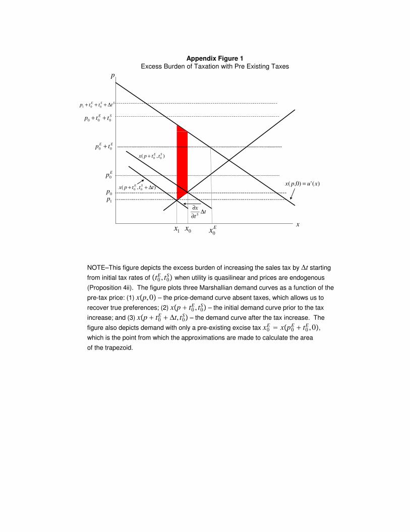
Appendix Figure 1

Excess Burden of Taxation with Pre Existing Taxes

p

x0

x

SEttp

000++

SSEtttp ∆+++

001

1x

0p

1p

Ep0

EEtp

00+

tt

xS

∆∂

∂

Ex

0

)(')0,( xupx =

),(00

SEttpx +

),( 00 tttpxSE

∆++

NOTE–This figure depicts the excess burden of increasing the sales tax by Δt starting

from initial tax rates of t0E, t0

S when utility is quasilinear and prices are endogenous

(Proposition 4ii). The figure plots three Marshallian demand curves as a function of the

pre-tax price: (1) xp, 0 – the price-demand curve absent taxes, which allows us to

recover true preferences; (2) xp + t0E, t0

S – the initial demand curve prior to the tax

increase; and (3) xp + t0E + Δt, t0

S – the demand curve after the tax increase. The

figure also depicts demand with only a pre-existing excise tax x0E = xp0

E + t0E, 0,

which is the point from which the approximations are made to calculate the area

of the trapezoid.

APPENDIX EXHIBIT 1: CLASSROOM SURVEY

Short survey on spending patterns

Major: _____________

Year: _____________

Gender: _____________

Choose two items from the image projected on the screen.

Number of item #1: ___________

Number of item #2: ___________

Total bill due at the register for these two items:

$_________

APPENDIX EXHIBIT 2: TAX SURVEY University of California, Berkeley

Department of Economics

This survey is part of a project about taxes being conducted by researchers at UC Berkeley. Your identity will be kept strictly confidential and will not be used in the research. If you have any questions about your rights or treatment as a participant in this research project, please contact UC-Berkeley’s Committee for Protection of Human Subjects at (510) 642-7461, or e-mail: subjects@berkeley.edu.

Gender:

Male

Female

Age:

Marital Status:

Married

Unmarried

Education: High School

College Degree

Graduate Degree

Years You Have Lived in California:

Is tax added at the register (in addition to the price posted on the shelf) for each of the following items?

milk Y N toothpaste Y N

magazines Y N soda Y N

beer Y N cookies Y N

potatoes Y N cigarettes Y N

Have you purchased these items within the last month? milk Y N toothpaste Y N

magazines Y N soda Y N

beer Y N cookies Y N

potatoes Y N cigarettes Y N

What is the sales tax rate in [city]? ___________%

What is the California state income tax rate in the highest tax bracket? _____________ %

What percentage of families in the US do you think pay the federal estate tax when someone dies?

< 2% 2-10% 10-25% 25-50% > 50% Thank you for your time!