Salient Assemblage Slide Presentation

Salient Assemblage Representation

of

Multidimensional, Recursive, Deforming

Geometry

William L. AndersonEleSoft Research

8727 Ellington Park Dr.Charlotte, NC 28277

704-543-9180Web and Email: www.elesoft.com

Copyright c© 1990-2008 by EleSoft Research. Allrights reserved.

1

Prototypical Salient Assemblage

Assemblage constructed from 3 salient units.

Concise data storage (24 constants)[3.0 0.0 1.0 0 0.0 0.0 1.0 02.0 0.0 0.5 0 0.0 0.5 0.5 02.0 0.5 0.2 0 0.0 0.5 0.2 0

]

2

Salient Assemblage Representation yr = f(xi)

Requirements

• Add, remove, reposition, deform salient units.

• Asymptotic C∞ salient blending.

• Topologically invariant, homeomorphic with

one parameter space.

• Local control of salient direction, shape,

size, and volume, at least approximately.

• Recursive attachment rules, like alignment

with principal directions.

• Applies to any dimension (i = 1,2, . . . , n).

3

Salient Assemblage is Topologically Invariant

Appended to Torus

4

Salient Assemblage Representation yr = f(xi)

Characteristics

• Constructive formulation, salient semiaxes

form finite skeleton substructure.

• Concise data storage.

• One patch, thus no patch boundary, avoid

geodesic cusp.

• Parameters usually have physical significance.

• Nowhere flat.

• Complicated algebraic expressions require

computer.

5

Applications

• Parametric Systems (multidimensional)

– Chemical reaction

– Economy

– Decision making

– Geodesic determination

• Geometric Modeling (shape sensitive)

– External fluid flow

– Biological surface, deformation, growth

– Telecommunicating complicated geom-

etry using concise data storage

6

Key Issues

• What notation? Tensor notation for gen-

eral curvilinear coordinate transformations.

• How to control salient direction, shape, and

size, at least approximately.

• Account for parameter stretching and co-

ordinate curve obliquity.

• Account for salient attachment in high-curvature

regions.

• Efficiently compute complicated algebraic

expressions.

7

Comparison with Other Mathematics

Frequently Asked Questions

• Why not conformal mapping? Powerful but toospecialized—requires analytic mapping, preserves an-gle, limited to 2 dimensions, corresponds to minimalsurfaces, a special class of manifolds. A salientshas less restrictive C∞ continuity and can be mul-tidimensional.

• Why not 3D modeling, partition into small splinepatches? Very complicated face, edge, and ver-tice relations in high dimensions. Patch boundariescomplicate geodesic computation.

• Why not use Fourier Transform, making period ar-bitrarily large? Salient is more natural, not definedby a integral.

• Why is a salient a tensor-product surface? Effi-cient evaluation and partial derivatives, and easilyextends to higher dimensions.

• Can a salient be a minimal surface? No. It hasnon-constant curvature. It is nowhere flat.

8

Comparison with Spline Representations

Assemblage Multi-patch Splinesprimitive salient splineformulation function discreterecursive yes notopology modeling invariant flexibleparameters physical arbitrarypatch coverage large smallpatch boundary C∞ C2

data storage salient constants control vertices

Both are parametric representations and are compatible.

9

Presentation Overview

1. Describe a salient.

2. Describe ExpHermite salient, a generalized

Fourier series.

3. Describe salient attachment rules.

4. Derive parametric representation yr = f(xi).

5. Apply differential geometry methods, e.g.

geodesics.

10

Definitions

Definition 1 A salient is the mathematical representa-tion of a distinguishable geometric part. It is a class C∞

bounded function on IR that, along with all its boundedderivatives, vanishes sufficiently far from one set of para-metric arguments.

y0

x1, y1

1D Salient

Definition 2 An assemblage is a collection of attachedsalients.

y0

x1, y1

1D Assemblage

11

1D Salient

y0

x1, y1

1D Salient

t��*

y0

x1, y1

Main Semiaxis Direction (Dihedral)

y0 = η0S,

y1 = x1 + η1S,

where ηr are direction cosines.

12

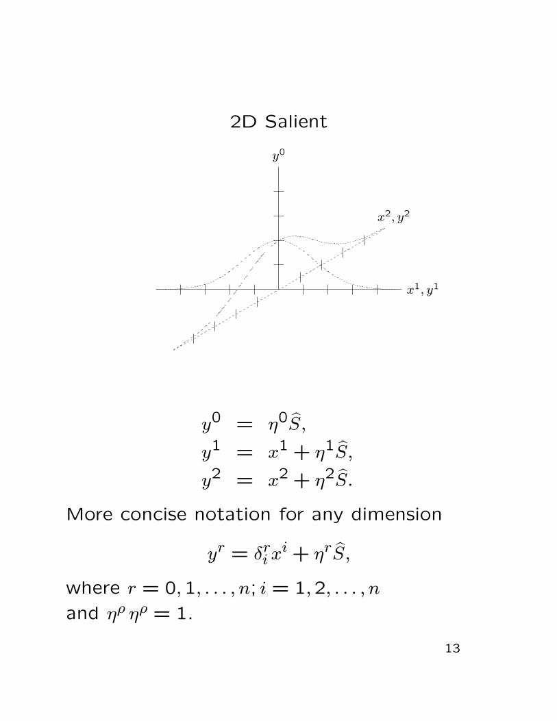
2D Salient

y0

x1, y1

x2, y2

y0 = η0S,

y1 = x1 + η1S,

y2 = x2 + η2S.

More concise notation for any dimension

yr = δri xi + ηrS,

where r = 0,1, . . . , n; i = 1,2, . . . , n

and ηρ ηρ = 1.

13

Salient Derivatives are Salients

SS;11S;12S;13

1D Salient and Its First Three Derivatives

If 1D salient S and its derivatives are linearlyindependent, then linear combination

S = c0S + c1S;1 + c2S;11 + · · ·+ cnhS;1nh

= chS;1h (sum on h = 0,1, . . . , nh).

spans a wider collection of 1D salients.

14

2D Salient

A linear combination of a 2D salient S(x1, x2)

and its derivatives

S = ch1h2S;1h12h2(x1, x2),

is also a 2D salient.

Consider only factorable S. Then S is a tensor-

product surface,

S =(ch1(1)S(1);1h1

(x1))· · ·

(chn(n)S(n);nhn (xn)

),

=∏j

chj(j)S(j);j

hj

(xj).

Consequently,

yr = δri xi + ηrS = δri x

i + ηr∏j

chj(j)S(j);j

hj

(xj).

15

Salient Nomenclaturey0

x1, y1

x2, y2

X(1)� -

X(2)*�

Although a salient is open and unbounded, ellipse nomen-clature is useful.

Definition 3 Salient origin, denoted by Xi, is the salient’slocal coordinate origin.

Local curvilinear coordinates, centered on salient origin,are

xi ≡ xi − Xi.

Definition 4 Salient main semiaxis is the line segmentfrom salient origin in direction ηr.

Definition 5 Salient height is main semiaxis length.

Definition 6 Salient vertex is main semiaxis endpoint.

Definition 7 Salient xj-semiaxis is the positive canon-ical coordinate xj axis.

Definition 8 Salient semiaxis width X(j) is the xj-semiaxisradial width at which salient height is 1/e times the mainsemiaxis height.

16

Local Curvilinear to Canonical Coordinate

Transformation

In two-dimensions, scaling and rotation trans-

formations are[x1

x2

]=

[1/X(1) 0

0 1/X(2)

] ζ11 ζ1

2

ζ21 ζ2

2

[ x1

x2

].

In any dimension,

xj = χjαζαi x

i.

17

2D Salient (Tensor-Product Surface) with

Two Shapes

Rectangle and Cone Approximations (5 terms)

In this case, salient semiaxes are rotated π/4

from rectangular axes.

18

Candidate Salient Functions

• exp(−x2

)

• 2 exp (x) /(1 + exp (2x))

• sin(ax)/x

• Bessel function J0(x)

• J1(x)/x

• sech(x)

• 1/(1 + ax2)

19

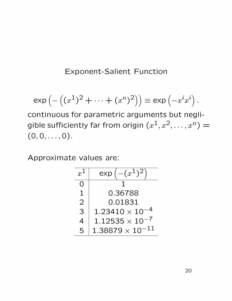
Exponent-Salient Function

exp(−((x1)2 + · · ·+ (xn)2

))≡ exp

(−xixi

).

continuous for parametric arguments but negli-

gible sufficiently far from origin (x1, x2, . . . , xn) =

(0,0, . . . ,0).

Approximate values are:

x1 exp(−(x1)2

)0 11 0.367882 0.018313 1.23410× 10−4

4 1.12535× 10−7

5 1.38879× 10−11

20

Hermite Polynomials

Exponent-salient function has derivatives of all

orders

dh

dxhexp

(−x2

)= exp

(−x2

)Hh (x) .

Definition 9 Hermite polynomials are

H0 (x) = 1,

H1 (x) = −2x,

Hh+1 (x) = −2(xHh (x) + hHh−1 (x)

).

First few Hermite Polynomials

H0 (x) = 1,

H1 (x) = −2x,

H2 (x) = −2 + 4x2,

H3 (x) = 12x− 8x3,

H4 (x) = 12− 48x2 + 16x4,

H5 (x) = −120x+ 160x3 − 32x5.

21

ExpHermite Series

Hermite polynomial products, weighted by exp(−x2

),

are orthogonal,∫ ∞−∞

exp(−x2

)Hh (x)Hθ (x) dx =

{0 if h 6= θ2hh!√π if h = θ.

Expand given salient function as an ExpHermite series

f(x) = exp(−x2

)chHh (x) (sum on h = 0,1, . . . , nh).

where ch are ExpHermite coefficients and the ExpHer-mite series is a generalized Fourier series. To find ch,multiply both sides by Hθ (x),

f(x)Hθ (x) = exp(−x2

)chHh (x)Hθ (x) .

Integrating both sides gives∫ ∞−∞

f(x)Hθ (x) dx = ch∫ ∞−∞

exp(−x2

)Hh (x)Hθ (x) dx.

Because of orthogonality, for any particular h,∫ ∞−∞

f(x)Hh (x) dx = ch∫ ∞−∞

exp(−x2

)(Hh (x))2 dx.

From first equation above,

ch =1

2hh!√π

∫ ∞−∞

f(x)Hh (x) dx.

22

ExpHermite Coefficients for Special Shapes

Using

ch =1

2hh!√π

∫ ∞−∞

f(x)Hh (x) dx,

determine coefficients:f(x) c0 c2 c4 c6

exponent exp(−x2)

1 0 0 0

rectangle 1 2√π

−16√π

−1240√π

2920160

√π

cone 1− |x| 1√π

−16√π

191440

√π

−1320160

√π

parabola 1− x2 43√π

−15√π

11840√π

−3790720

√π

semicircle√

1− x2√π

2−√π

16

√π

384

√π

18432

These shapes are even functions with unit

height and unit semiaxis width.

23

Approximation by ExpHermite Series

Rectangle

f(x) =

{0 if x < −11 if − 1 ≤ x ≤ 10 if x > 1,

is approximated by

f(x) ≈exp(−x2)

√π

(2−

1

6H2(x)−

1

240H4(x) +

29

20160H6(x)

−67

580608H8(x)

).

To compute, transform to power series

f(x) ≈ exp(−x2) (

(((−0.01667x2 + 0.28528)x2 − 1.30219)x2

+ 1.19607)x2 + 1.08147).

y0

x1, y1

24

Approximation by ExpHermite Series

Cone approximation (5 terms)

f(x) =

{0 if x < −11− |x| if − 1 ≤ x ≤ 10 if x > 1.

y0

x1, y1

Parabola approximation (5 terms)

f(x) =

{0 if x < −11− x2 if − 1 ≤ x ≤ 10 if x > 1.

y0

x1, y1

25

2D Ramp Approximation by Tensor-Product

of ExpHermite Series

26

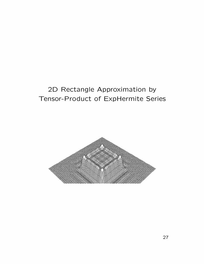
2D Rectangle Approximation by

Tensor-Product of ExpHermite Series

27

ExpHermite Series Successive Approximations

Change Shape but not Volume

Since ∫ ∞−∞

exp(−x2

)dx =

√π,

and for h > 0,∫ ∞−∞

exp(−x2

)Hh (x) dx = 0,

then volume V under approximating surface is

V =∫X

exp (−xγxγ)∏j

chj(j)Hhj

(xj)dx1 · · · dxn,

=

∏j

c0(j)

∫X

exp (−xγxγ) dx1 · · · dxn,

= πn/2∏j

c0(j).

28

Assemblage Definitions

Definition 10 An assemblage is a collection

of attached salients.

Definition 11 A salient’s parent is the assem-

blage to which it is attached.

Definition 12 A salient is a child to its par-

ent.

Definition 13 A child’s bud is the point Y r =

yr(Xi), located on the parent.

Definition 14 A child’s dihedral is the mini-

mum angle its main semiaxis forms with the

parent’s tangent plane at the bud.

29

Salient Attachment by Vector Addition

bark

tbark-bud

t6bark-bud-branch

t��7bark-bud-branch

tCCO

bark-bud-branch

Each salient depends on all its parents.

t6t - t���t�tCCO

y0

x1, y1

30

Salient Direction Cosine (Dihedral) Rule

The mth salient main semiaxis can have any

direction ηrm, but usually is either:

• parent’s unique normal vector,

• branch angle, coplanar with parent’s posi-

tive main semiaxis,

• fixed angle to rectangular axes yr.

Rule can be an inherited.

t6t - t���t�tCCO

y0

x1, y1

31

Parameter Stretching and Coordinate Curve

Obliquity

y0

x1, y1

Child Salients Affected by Parameter Stretching

Coordinate Curve Obliquity

32

Arc-Length and Oblique Coordinate

Transformations

Given by metric tensor gij at salient origin.

Arc-length coordinate transformation (2D)

[λεi ] =

[ √g11 00

√g22

].

Oblique coordinate transformation (2D)

[ωγε ] =

1 g12√

g11√g22

0

√1− (g12)2

g11g22

,

from Gramm-Schmidt orthonormalization.

33

Semiaxis Alignment Coordinate

Transformation

Semiaxes are aligned with either:

• principal directions at bud, eigenvectors of

[biα] [xα] = κ [giα] [xα] .

• branch angle direction, in the normal sec-

tion that is parallel to the parent’s positive

main semiaxis,

• fixed direction relative to rectangular axes

yr,

• one coordinate curve tangent vector.

Rule can be an inherited.34

Salient Addition

Salient addition is closed.

Addition of a coupled salient is non-commutative

and non-associative.

t6tPPi

t6 t���

y0

x1, y1

Non-commutative Salient Addition

35

Salient Attachment in High-Curvature

Regions

Definition 15 If child salient is smaller, the

interaction is hierarchical or tree-like.

Definition 16 If child salient is approximately

the same size or larger, the interaction is tumor-

like, or if flattened anvil-like.

t6t�

t6

t -y0

x1, y1

Tree-like and Tumor-like Salient Interaction

Two widely separated salients m1 and m2 are

approximately orthogonal,∫IRn|Sm1 Sm2| dx1 dx2 · · · dxn ≈ 0.

36

Salient Assemblage Representation

Overall coordinate transformation

Υj(m)i ≡ χ

j(m)αζ

α(m)βς

β(m)γω

γ(m)ελ

ε(m)i.

Canonical coordinates

xj(m) = Υj

(m)i

(xi − Xi

(m)

).

Parametric representation

yr = δri xi + ηrmS

m,

= δri xi + ηrm

∏j

chj(mj)S

m

(j);jhj

(xj(m)

).

First partial derivative

yr,k = δrk + ηrmΥα(m)kS

m,α,

= δrk + ηrmΥα(m)k

∏j

chj(mj)S

m

(j);jhj+δα

j

(xj(m)

).

Second partial derivative

yr,kl = ηrmΥα(m)kΥβ

(m)lSm,αβ,

= ηrmΥα(m)kΥβ

(m)l

∏j

chj(mj)S

m

(j);jhj+δα

j+δ

βj

(xj(m)

).

37

1D ExpHermite Assemblage

ExpHermite salients in the form

Sm = expm(−(x1

(m))2)ch(m)Hh

(x1

(m)

).

combine to form assemblage like

Cone, Parabola, and Rectangle in Tree

38

ExpHermite Salient Assemblage

Representation

Parametric representation

yr = δri xi + ηrm expm

(−xγ

(m)xγ

(m)

)∏j

chj(mj)

Hhj

(xj

(m)

).

First partial derivative

yr,k = δrk + ηrmΥα(m)k expm

(−xγ

(m)xγ

(m)

)∏j

chj(mj)

Hhj+δαj

(xj

(m)

).

Second partial derivative

yr,kl = ηrmΥα(m)kΥ

β(m)l

expm(−xγ

(m)xγ

(m)

)∏j

chj(mj)

Hhj+δαj

+δβj

(xj

(m)

).

39

Global Cylindrical Coordinates

(ρ, θ, z) to rectangular yr

y0 = z,

y1 = ρ cos θ,

y2 = ρ sin θ.

Inverse transformation

z = y0,

ρ =√

(y1)2 + (y2)2,

θ = tan−1(y2/y1

).

Global cylinder ρ = R is

x1 = R sin θ,

x2 = z.

Global point (Θ, Z) becomes m0 salient origin

X1(0) = R sin Θ(0),

X2(0) = Z(0).

40

Global Spherical-Polar Coordinates

(ρ, φ, θ) to rectangular yr

y0 = ρ cosφ,

y1 = ρ sinφ cos θ,

y2 = ρ sinφ sin θ.

Inverse transformation

ρ =√

(y0)2 + (y1)2 + (y2)2,

φ = tan−1(√

(y1)2 + (y2)2/y0),

θ = tan−1(y2/y1

).

Global sphere ρ = R is

x1 = R sinφ cos θ,

x2 = R sinφ sin θ,

Global point (Θ, Φ) becomes m0 salient origin

X1(0) = R sin Φ(0) cos Θ(0),

X2(0) = R sin Φ(0) sin Θ(0).

41

Assemblage Self-Intersection

t6t��1

t6tPPi

y0

x1, y1

Position vectors yr of main semiaxes:

yr(m1) = Y r(m1) + t1η

r(m1),

yr(m2) = Y r(m2) + t2η

r(m2),

where Y r(m1)

and Y r(m2)

are buds, and t1 and t2 are scalar real param-

eters. Perpendicular connecting vector(yr(m1) − yr(m2)

)ηr(m1) = 0,(

yr(m1) − yr(m2))ηr(m2) = 0.

So [ηr

(m1)ηr(m1)

−ηr(m2)

ηr(m1)

ηr(m1)

ηr(m2)

−ηr(m2)

ηr(m2)

][t1t2

]=[

−(Y r(m1)− Y r

(m2))η

r(m1)

−(Y r(m1)− Y r

(m2))η

r(m2)

]

42

Concise Data Storage

Salient-constant array for 2D assemblagec

(0)X1

(0)X(1)

(0)shape1

(0) ζ(0)

X2(0)

X(2)(0)

shape2(0)

c(1)

X1(1)

X(1)(1)

shape1(1) ζ

(1)X2

(1)X(2)

(1)shape2

(1)

c(2)

X1(2)

X(1)(2)

shape1(2) ζ

(2)X2

(2)X(2)

(2)shape2

(2)...

......

......

......

...

One row for each salient.

Facilitate telecommunicating a complicated ge-

ometry.

43

Efficient Computation

Assemblage

• Predict negligible terms from parameter values.

• Univariate factors in tensor-product.

• If recursive formula exists and is more efficient, useit.

• For non-deforming, precompute assemblage con-stants.

• For non-deforming, precompute coupling matrix.

• For partial derivatives, reuse previously computedfunction evaluations and repeating chain-rule fac-tors.

ExpHermite Assemblage

• Exponent function exp(−x2

)factors out, leaving

efficient polynomial.

• Transform Hermite series to power series.

• If factor is even or odd function, half the terms arezero and can be bypassed.

44

Transform Hermite Series to Power Series

Hermite series has equivalent power series

dqj(mj)δαj hk

Pqj

(xj(m)

)= c

hj(mj)Hhj+δαj hk

(xj(m)

),

where

Pqj

(xj(m)

)≡(xj(m)

)qj.

Coefficients transform as

dqj(mj)hk

= $qjϑ δ

ϑθ+hk

cθ(mj),

where

[$qjϑ

]=

1 0 −2 0 120 −2 0 12 00 0 4 0 −480 0 0 −8 00 0 0 0 16

.. .

.

Multiplication δϑθ+hkcθ(mj) is equivalent to a shift

of array c elements.

45

Differential Geometry

Parametric representation and its first two par-

tial derivatives

yr, yr,k, yr,kl.

Jacobian matrix

J ≡ [Jri ](n+1)×n ≡ yr,i.

Base vectors are functions of position (curvi-

linear coordinates)

ai = y,i ≡ yρ,ieρ.

Metric tensor

gij ≡ ai aj.

Since yr are rectangular coordinates with the

Euclidean metric,[gij]

= JTJ =[yρ,i y

ρ,j

].

46

Differential Geometry

A more general Riemannian metric, including

non-Euclidean, is[gij]

= JTGJ.

If J is full rank, then there exists a gij such

that

giα gαj = δij.

Metric tensor determinant

g ≡ |gij|.

For two dimensions, g = g11g22 − (g12)2.

Cosine between xi and xj-parametric curves

cosω = gij/√gii gjj (no sum on i, j).

Invariant First Fundamental Form

I ≡ gijdxi dxj.

47

Differential Geometry

Christoffel symbols of the first kind

Γijk ≡1

2

(gjk,i + gki,j − gij,k

).

With rectangular coordinates yr and Euclidean

metric

Γijk = yρ,k y

ρ,ij.

Christoffel symbols of the second kind

Γkij ≡ gkαΓijα.

Riemannian tensor of the second kind

Rijkl ≡ Γijl,k − Γijk,l + ΓαjlΓiαk − ΓαjkΓiαl.

Riemannian tensor of the first kind

Rijkl ≡ giαRαjkl.

Gaussian curvature on a two-dimensional sur-

face

K =R1212

g11g22 − (g12)2.

48

Differential Geometry

Surface curve, function of parameter t,

xi ≡ xi(t),

in ambient coordinates yr, is composite func-

tion

yr ≡ yr(xi(t)).

Curve’s tangent is given by chain-rule

dyr

dt= yr,i

dxi

dt.

Square of differential arc length is

(ds)2 = gij dxi dxj.

Curve arc length is

s =∫ x1

x0

√gij dx

i dxj =∫ t1t0

√gij

dxi

dt

dxj

dtdt.

Two-dimensional surface area is

A =∫X

√g dx1 dx2.

49

Geodesic

A geodesic xi(s) solves system of differential equations

d2xk

ds2+ Γk

ij

dxi

ds

dxj

ds= 0.

Geodesic on surface (http://www.netlib.org/ode/geodesic/)

Geodesic in parameter space

50

Differential Geometry

Surface normal vector

Nr = εrst ys,1 y

t,2.

Unit normal vector

nr ≡ Nr/√NρNρ.

Invariant Second Fundamental Form

II ≡ bijdxi dxj,

with coefficients from curvature tensor

bij ≡ yρ,ijnρ.

For two dimensions,

b ≡ |bij| = b11b22 − (b12)2.

Gauss equation

yr,ij = Γαij yr,α + bijn

r.

Weingarten equation

nr,i = −gαβbiαyr,β = −bβi yr,β.

51

Tensor Applications

Newton’s second law

F r = mdvr

dt,

= m

(d2yr

dt2+ Γrij

dxi

dt

dxj

dt

),

is valid in all coordinate systems.

Describes a force field on a curved surface, like

the interface between two fluids.

52

Potential Flow Examples

y0

x1, y1

x2, y2

-

-

-

-

-

U∞

-

U∞

Potential Flow over Plane: φ = −U∞x2

y0

x1, y1

x2, y2

-

-

-

-

-

U∞-

2U∞

Potential Flow over Cylinder: φ = −U∞(

1 + R2

r2

)r cos θ

53

Potential Flow Examples

y0

x1, y1

x2, y2

-

-

-

-

-

U∞-

1.5U∞

Potential Flow over Sphere: φ = −U∞(

1 + R3

2r3

)r cos θ

y0

x1, y1

x2, y2

-

-

-

-

-

U∞-

?

Potential Flow over Salient

54

Conclusions

Salient assemblage representation is important because:

• Complexity of many problems stems from repre-sentation of irregular or deforming geometry. Anassemblage decomposes a geometric object intoasymptotic blending salient units. It models a mul-tidimensional parametric system.

• A linear combination of a 1D salient and its deriva-tives spans a wider collection of 1D salients.

• Salients are attached with recursive rules on dihe-dral and semiaxis alignment.

• An assemblage covers the surface of interest withone patch.

• An assemblage has concise data storage.

• It allows efficient computation.

ExpHermite assemblage representation has advantages:

• Built-in data fitting using ExpHermite series, a gen-eralized Fourier series.

• Efficient polynomial computation.

55