sample average approximation method for chance constrained
TRANSCRIPT
Sample Average Approximation Method
for Chance Constrained Programming:
Theory and Applications
B.K. Pagnoncelli∗ S. Ahmed† A. Shapiro ‡
Communicated by P.M. Pardalos
Abstract
We study sample approximations of chance constrained problems. In partic-
ular, we consider the sample average approximation (SAA) approach and discuss
the convergence properties of the resulting problem. We discuss how one can
use the SAA method to obtain good candidate solutions for chance constrained
∗(�)Departamento de Matematica, Pontifıcia Universidade Catolica do Rio de Janeiro, Rio deJaneiro, RJ Brazil 22453-900, e-mail: [email protected], research supported by CAPES andFUNENSEG.
†Georgia Institute of Technology, Atlanta, Georgia 30332, USA, e-mail: [email protected],research of this author was partly supported by the NSF award DMI-0133943.
‡Georgia Institute of Technology, Atlanta, Georgia 30332, USA, e-mail:[email protected], research of this author was partly supported by the NSF awardDMI-0619977.
1

problems. Numerical experiments are performed to correctly tune the parameters
involved in the SAA. In addition, we present a method for constructing statistical
lower bounds for the optimal value of the considered problem and discuss how one
should tune the underlying parameters. We apply the SAA to two chance con-
strained problems. The first is a linear portfolio selection problem with returns
following a multivariate lognormal distribution. The second is a joint chance
constrained version of a simple blending problem.
Key words: Chance constraints, Sample average approximation, Portfolio selection.
1 Introduction
We consider chance constrained problems of the form
minx∈X
f(x), s.t. prob{
G(x, ξ) ≤ 0}
≥ 1 − α. (1)
Here X ⊂ Rn, ξ is a random vector1 with probability distribution P supported on a
set Ξ ⊂ Rd, α ∈ (0, 1), f : R
n → R is a real valued function and G : Rn × Ξ → R
m.
Chance constrained problems were introduced in Charnes, Cooper and Symmonds [1]
1We use the same notation ξ to denote a random vector and its particular realization. Which ofthese two meanings will be used in a particular situation will be clear from the context.
2

and have been extensively studied since. For a theoretical background we may refer
to Prekopa [2] where an extensive list of references can be found. Applications of
chance constrained programming include, e.g., water management [3] and optimization
of chemical processes [4],[5].
Although chance constraints were introduced almost 50 years ago, little progress
was made until recently. Even for simple functions G(·, ξ), e.g., linear, problem (1) may
be extremely difficult to solve numerically. One of the reasons is that for a given x ∈ X
the quantity prob {G(x, ξ) ≤ 0} is hard to compute since it requires a multi-dimensional
integration. Thus, it may happen that the only way to check feasibility, of a given
point x ∈ X, is by Monte-Carlo simulation. In addition, the feasible set of problem
(1) can be nonconvex even if the set X is convex and the function G(x, ξ) is convex
in x. Therefore the development went into two somewhat different directions. One
is to discretize the probability distribution P and consequently to solve the obtained
combinatorial problem (see, e.g., Dentcheva, Prekopa and Ruszczynski [6], Luedtke,
Ahmed and Nemhauser [7]). Another approach is to employ convex approximations of
chance constraints (cf., Nemirovski and Shapiro [8]).
In this paper we discuss the sample average approximation (SAA) approach to
chance constrained problems. Such an approximation is obtained by replacing the actual
3

distribution in chance constraint by an empirical distribution corresponding to a random
sample. This approach is well known for stochastic programs with expected values
objectives [9]. SAA methods for chance constrained problems have been investigated
in [10] and [11].
The remainder of the paper is organized as follows. In Section 2 we provide theoret-
ical background for the SAA approach, showing convergence of the optimal value of the
approximation to the optimal value of the true problem. In addition, following [8] we
describe how to construct bounds for the optimal value of chance constrained problems
of the form (1). In Section 3, we present a chance constrained portfolio selection prob-
lem. We apply the SAA method to obtain upper bounds as well as candidate solutions
to the problems. In addition we present several numerical experiments that indicate
how one should tune the parameters of the SAA approach. In Section 4 we present
a simple blending problem modeled as a joint chance constrained problem. Section 5
concludes the paper and suggests directions for future research.
We use the following notation throughout the paper. The integer part of number
a ∈ R is denoted by ⌊a⌋. By Φ(z) we denote the cumulative distribution function (cdf)
of standard normal random variable and by zα the corresponding critical value, i.e.,
4

Φ(zα) = 1 − α, for α ∈ (0, 1),
B(k; p,N) :=∑k
i=0
(
N
i
)
pi(1 − p)N−i, k = 0, ..., N, (2)
denotes the cdf of binomial distribution. For sets A,B ⊂ Rn we denote by
D(A,B) := supx∈A dist(x,B) (3)
the deviation of set A from set B.
2 Theoretical Background
In order to simplify the presentation we assume in this section that the constraint
function G : Rn×Ξ → R is real valued. Of course, a number of constraints Gi(x, ξ) ≤ 0,
i = 1, . . . , m, can be equivalently replaced by one constraint with
G(x, ξ) := max1≤i≤m
Gi(x, ξ) ≤ 0.
Such operation of taking maximum preserves convexity of functions Gi(·, ξ). We assume
that the set X is closed, the function f(x) is continuous and the function G(x, ξ) is a
5
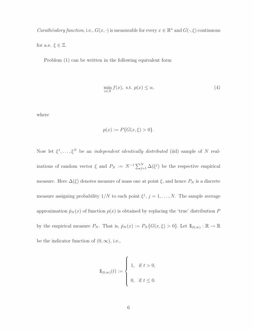
Caratheodory function, i.e., G(x, ·) is measurable for every x ∈ Rn andG(·, ξ) continuous
for a.e. ξ ∈ Ξ.
Problem (1) can be written in the following equivalent form
minx∈X
f(x), s.t. p(x) ≤ α, (4)
where
p(x) := P{G(x, ξ) > 0}.
Now let ξ1, . . . , ξN be an independent identically distributed (iid) sample of N real-
izations of random vector ξ and PN := N−1∑N
j=1 ∆(ξj) be the respective empirical
measure. Here ∆(ξ) denotes measure of mass one at point ξ, and hence PN is a discrete
measure assigning probability 1/N to each point ξj, j = 1, . . . , N . The sample average
approximation pN(x) of function p(x) is obtained by replacing the ‘true’ distribution P
by the empirical measure PN . That is, pN(x) := PN{G(x, ξ) > 0}. Let 1l(0,∞) : R → R
be the indicator function of (0,∞), i.e.,
1l(0,∞)(t) :=
1, if t > 0,
0, if t ≤ 0.
6

Then we can write that p(x) = EP [1l(0,∞)(G(x, ξ))] and
pN (x) = EPN[1l(0,∞)(G(x, ξ))] =
1
N
N∑
j=1
1l(0,∞)
(
G(x, ξj))
.
That is, pN(x) is equal to the proportion of times that G(x, ξj) > 0. The problem,
associated with the generated sample ξ1, . . . , ξN , is
minx∈X
f(x), s.t. pN(x) ≤ γ. (5)
We refer to problems (4) and (5) as the true and SAA problems, respectively, at the
respective significance levels α and γ. Note that, following [11], we allow the significance
level γ ≥ 0 of the SAA problem to be different from the significance level α of the true
problem. Next we discuss the convergence of a solution of the SAA problem (5) to that
of the true problem (4) with respect to the sample size N and the significance level γ.
A convergence analysis of the SAA problem (5) has been given in [11]. Here we present
complementary results under slightly different assumptions.
Recall that a sequence fk(x) of extended real valued functions is said to epiconverge
to a function f(x), written fke→ f , if for any point x the following two conditions hold:
7

(i) for any sequence xk converging to x one has
lim infk→∞
fk(xk) ≥ f(x), (6)
(ii) there exists a sequence xk converging to x such that
lim supk→∞
fk(xk) ≤ f(x). (7)
Note that by the (strong) law of large numbers (LLN) we have that for any x, pN(x)
converges w.p.1 to p(x).
Proposition 2.1 Let G(x, ξ) be a Caratheodory function. Then the functions p(x) and
pN(x) are lower semicontinuous, and pNe→ p w.p.1. Moreover, suppose that for every
x ∈ X the set {ξ ∈ Ξ : G(x, ξ) = 0} has P -measure zero, i.e., G(x, ξ) 6= 0 w.p.1.
Then the function p(x) is continuous at every x ∈ X and pN(x) converges to p(x) w.p.1
uniformly on any compact set C ⊂ X, i.e.,
supx∈C
|pN(x) − p(x)| → 0 w.p.1 as N → ∞. (8)
Proof. Consider function ψ(x, ξ) := 1l(0,∞)
(
G(x, ξ))
. Recall that p(x) = EP [ψ(x, ξ)]
8

and pN(x) = EPN[ψ(x, ξ)]. Since the function 1l(0,∞)(·) is lower semicontinuous and
G(·, ξ) is a Caratheodory function, it follows that the function ψ(x, ξ) is random lower
semicontinuous2 (see, e.g., [12, Proposition 14.45]). Then by Fatou’s lemma we have
for any x ∈ Rn,
lim infx→x p(x) = lim infx→x
∫
Ξψ(x, ξ)dP (ξ)
≥∫
Ξlim infx→x ψ(x, ξ)dP (ξ) ≥
∫
Ξψ(x, ξ)dP (ξ) = p(x).
This shows lower semicontinuity of p(x). Lower semicontinuity of pN(x) can be shown
in the same way.
The epiconvergence pNe→ p w.p.1 is a direct implication of Artstein and Wets [13,
Theorem 2.3]. Note that, of course, |ψ(x, ξ)| is dominated by an integrable function
since |ψ(x, ξ)| ≤ 1. Suppose, further, that for every x ∈ X, G(x, ξ) 6= 0 w.p.1, which
implies that ψ(·, ξ) is continuous at x w.p.1. Then by the Lebesgue Dominated Con-
vergence Theorem we have for any x ∈ X,
limx→x p(x) = limx→x
∫
Ξψ(x, ξ)dP (ξ)
=∫
Ξlimx→x ψ(x, ξ)dP (ξ) =
∫
Ξψ(x, ξ)dP (ξ) = p(x),
which shows continuity of p(x) at x = x. Finally, the uniform convergence (8) follows
2Random lower semicontinuous functions are called normal integrands in [12].
9
by a version of the uniform law of large numbers (see, [9, Proposition 7, p.363]).
By lower semicontinuity of p(x) and pN(x) we have that the feasible sets of the
‘true’ problem (4) and its SAA counterpart (5) are closed sets. Therefore, if the set
X is bounded (i.e., compact), then problems (4) and (5) have nonempty sets of opti-
mal solutions denoted, respectively, as S and SN , provided that these problems have
nonempty feasible sets. We also denote by ϑ∗ and ϑN the optimal values of the true
and the SAA problems, respectively. The following result shows that for γ = α, under
mild regularity conditions, ϑN and SN converge w.p.1 to their counterparts of the true
problem.
We make the following assumption.
(A) There is an optimal solution x of the true problem (4) such that for any ε > 0
there is x ∈ X with ‖x− x‖ ≤ ε and p(x) < α.
In other words the above condition (A) assumes existence of a sequence {xk} ⊂ X
converging to an optimal solution x ∈ S such that p(xk) < α for all k, i.e., x is an
accumulation point of the set {x ∈ X : p(x) < α}.
Proposition 2.2 Suppose that the significance levels of the true and SAA problems are
the same, i.e., γ = α, the set X is compact, the function f(x) is continuous, G(x, ξ) is
10

a Caratheodory function, and condition (A) holds. Then ϑN → ϑ∗ and D(SN , S) → 0
w.p.1 as N → ∞.
Proof. By the condition (A), the set S is nonempty and there is x ∈ X such that
p(x) < α. We have that pN(x) converges to p(x) w.p.1. Consequently pN(x) < α, and
hence the SAA problem has a feasible solution, w.p.1 for N large enough. Since pN (·)
is lower semicontinuous, the feasible set of SAA problem is compact, and hence SN is
nonempty w.p.1 for N large enough. Of course, if x is a feasible solution of an SAA
problem, then f(x) ≥ ϑN . Since we can take such point x arbitrary close to x and f(·)
is continuous, we obtain that
lim supN→∞
ϑN ≤ f(x) = ϑ∗ w.p.1. (9)
Now let xN ∈ SN , i.e., xN ∈ X, pN(xN ) ≤ α and ϑN = f(xN ). Since the set X is
compact, we can assume by passing to a subsequence if necessary that xN converges to
a point x ∈ X w.p.1. Also we have that pNe→ p w.p.1, and hence
lim infN→∞
pN(xN ) ≥ p(x) w.p.1.
It follows that p(x) ≤ α and hence x is a feasible point of the true problem, and thus
11

f(x) ≥ ϑ∗. Also f(xN) → f(x) w.p.1, and hence
lim infN→∞
ϑN ≥ ϑ∗ w.p.1. (10)
It follows from (9) and (10) that ϑN → ϑ∗ w.p.1. It also follows that the point x is an
optimal solution of the true problem and then we have D(SN , S) → 0 w.p.1.
Condition (A) is essential for the consistency of ϑN and SN . Think, for example,
about a situation where the constraint p(x) ≤ α defines just one feasible point x such
that p(x) = α. Then arbitrary small changes in the constraint pN(x) ≤ α may result in
that the feasible set of the corresponding SAA problem becomes empty. Note also that
condition (A) was not used in the proof of inequality (10). Verification of condition (A)
can be done by ad hoc methods.
Suppose now that γ > α. Then by Proposition 2.2 we may expect that with increase
of the sample size N , an optimal solution of the SAA problem will approach an optimal
solution of the true problem with the significance level γ rather than α. Of course,
increasing the significance level leads to enlarging the feasible set of the true problem,
which in turn may result in decreasing of the optimal value of the true problem. For a
point x ∈ X we have that pN(x) ≤ γ, i.e., x is a feasible point of the SAA problem, iff
12

no more than γN times the event “G(x, ξj) > 0” happens in N trials. Since probability
of the event “G(x, ξj) > 0” is p(x), it follows that
prob{
pN(x) ≤ γ}
= B(
⌊γN⌋; p(x), N)
. (11)
Recall that by Chernoff inequality [14], for k > Np,
B(k; p,N) ≥ 1 − exp{
−N(k/N − p)2/(2p)}
.
It follows that if p(x) ≤ α and γ > α, then 1 − prob{
pN(x) ≤ γ}
approaches zero at
a rate of exp(−κN), where κ := (γ − α)2/(2α). Of course, if x is an optimal solution
of the true problem and x is feasible for the SAA problem, then ϑN ≤ ϑ∗. That is, if
γ > α, then the probability of the event “ϑN ≤ ϑ∗” approaches one exponentially fast.
Similarly, we have that if p(x) = α and γ < α, then probability that x is a feasible
point of the corresponding SAA problem approaches zero exponentially fast (cf., [11]).
In order to get a lower bound for the optimal value ϑ∗ we proceed as follows. Let
13

us choose two positive integers M and N , and let
θN := B(
⌊γN⌋;α,N)
and L be the largest integer such that
B(L− 1; θN ,M) ≤ β. (12)
Next generate M independent samples ξ1,m, . . . , ξN,m, m = 1, . . . ,M , each of size N , of
random vector ξ. For each sample solve the associated optimization problem
minx∈X
f(x), s.t.
N∑
j=1
1l(0,∞)
(
G(x, ξj,m))
≤ γN, (13)
and hence calculate its optimal value ϑmN , m = 1, . . . ,M . That is, solve M times the
corresponding SAA problem at the significance level γ. It may happen that problem
(13) is either infeasible or unbounded from below, in which case we assign its optimal
value as +∞ or −∞, respectively. We can view ϑmN , m = 1, . . . ,M , as an iid sample of
the random variable ϑN , where ϑN is the optimal value of the respective SAA problem
at significance level γ. Next we rearrange the calculated optimal values in the nonde-
14

creasing order as follows ϑ(1)N ≤ · · · ≤ ϑ
(M)N , i.e., ϑ
(1)N is the smallest, ϑ
(2)N is the second
smallest etc, among the values ϑmN , m = 1, . . . ,M . We use the random quantity ϑ
(L)N as
a lower bound of the true optimal value ϑ∗. It is possible to show that with probability
at least 1 − β, the random quantity ϑ(L)N is below the true optimal value ϑ∗, i.e., ϑ
(L)N
is indeed a lower bound of the true optimal value with confidence at least 1 − β (see3
[8]). We will discuss later how to choose the constants M,N and γ.
3 A Chance Constrained Portfolio Problem
Consider the following maximization problem subject to a single chance constraint
maxx∈X
E[
rTx]
, s.t. prob{
rTx ≥ v}
≥ 1 − α. (14)
Here x ∈ Rn is vector of decision variables, r ∈ R
n is a random (data) vector (with
known probability distribution), v ∈ R and α ∈ (0, 1) are constants, e is a vector whose
components are all equal to 1 and
X := {x ∈ Rn : eTx = 1, x ≥ 0}.
3In [8] this lower bound was derived for γ = 0. It is straightforward to extend the derivations tothe case of γ > 0.
15

Note that, of course, E[
rTx]
= rTx, where r := E[r] is the corresponding mean vector.
That is, the objective function of problem
The motivation to study (14) is the portfolio selection problem going back to
Markowitz [15]. The vector x represents the percentage of a total wealth of one dol-
lar invested in each of n available assets, r is the vector of random returns of these
assets and the decision agent wants to maximize the mean return subject to having a
return greater or equal to a desired level v, with probability at least 1 − α. We note
that problem (14) is not realistic because it does not incorporate crucial features of
real markets such as cost of transactions, short sales, lower and upper bounds on the
holdings, etc. However, it will serve to our purposes as an example of an application of
the SAA method. For a more realistic model we can refer the reader, e.g., to [16].
3.1 Applying the SAA
First assume that r follows a multivariate normal distribution with mean vector r and
covariance matrix Σ, written r ∼ N (r,Σ). In that case rTx ∼ N(
rTx, xT Σx)
, and
hence (as it is well known) the chance constraint in (14) can be written as a convex
second order conic constraint (SOCC). Using the explicit form of the chance constraint,
one can efficiently solve the convex problem (14) for different values of α. An efficient
16
frontier of portfolios can be constructed in an objective function value versus confidence
level plot, that is, for every confidence level α we associate the optimal value of problem
(14). The efficient frontier dates back to Markowitz [15].
If r follows a multivariate lognormal distribution, then no closed form solution is
available. The sample average approximation (SAA) of problem (14) can be written as
maxx∈X
rTx, s.t. pN(x) ≤ γ, (15)
where
pN(x) := N−1
N∑
i=1
1l(0,∞)(v − rTi x)
and γ ∈ [0, 1). The reason we use γ instead of α is to suggest that for a fixed α, a
different choice of the parameter γ in (15) might be suitable. For instance, if γ = 0,
then the SAA problem (15) becomes the linear program
maxx∈X
rTx, s.t. rTi x ≥ v, i = 1, . . . , N. (16)
A recent paper by Campi and Garatti [17], building on the work of Calafiore and Campi
[18], provides an expression for the probability of an optimal solution xN of the SAA
17

problem (5), with γ = 0, to be infeasible for the true problem (4). That is, under the
assumptions that the set X and functions f(·) and G(·, ξ), ξ ∈ Ξ, are convex and that
w.p.1 the SAA problem attains unique optimal solution, we have that for N ≥ n,
prob {p(xN) > α} ≤ B(n− 1;α,N), (17)
and the above bound is tight. Thus, for a confidence parameter β ∈ (0, 1) and a sample
size N∗ such that
B(n− 1;α,N∗) ≤ β, (18)
the optimal solution of problem (16) is feasible for the corresponding true problem (14)
with probability at least 1 − β.
For γ > 0, problem (15) can be written as the mixed-integer linear program
maxx,z
rTx, (19a)
s.t. rTi x+ vzi ≥ v, (19b)
N∑
i=1
zi ≤ Nγ, (19c)
x ∈ X, z ∈ {0, 1}N , (19d)
18

with one binary variable for each sample point. To see that problems (15) and (19) are
equivalent, let (x, z1, . . . , zN) be feasible for problem (19). Then from the first constraint
of (19) we have zi ≥ 1l(0,∞)(v− rTi x), and so from the second constraint of (19) we have
γ ≥ N−1
N∑
i
zi ≥ N−11l(0,∞)(v − rTi x) = pN(x). (20)
Thus x is feasible to (15) and has the same objective value as in (19). Conversely, let x
be feasible for problem (15). Defining zi = 1l(0,∞)(v − rTi x), i = 1, . . . , N , we have that
(x, z1, . . . , zN ) is feasible for problem (19) with the same objective value.
Given a fixed α in (14), it is not clear what are the best choices of γ and N for (19).
We believe it is problem dependent and numerical investigations will be performed with
different values of both parameters. We know from Proposition 2.2 that, for γ = α the
larger the N the closer we are to the original problem (14). However, the number of
samples N must be chosen carefully because problem (19) is a binary problem. Even
moderate values of N can generate instances that are very hard to solve.
3.2 Finding Candidate Solutions
First we perform numerical experiments for the SAA method with γ = 0 (problem (16))
assuming that r ∼ N (r,Σ). We considered 10 assets (n = 10) and the data for the
19
estimation of the parameters was taken from historical monthly returns of 10 US major
companies. We wrote the codes in GAMS and solved the problems using CPLEX 9.0.
The computer was a PC with an Intel Core 2 processor and 2GB of RAM.
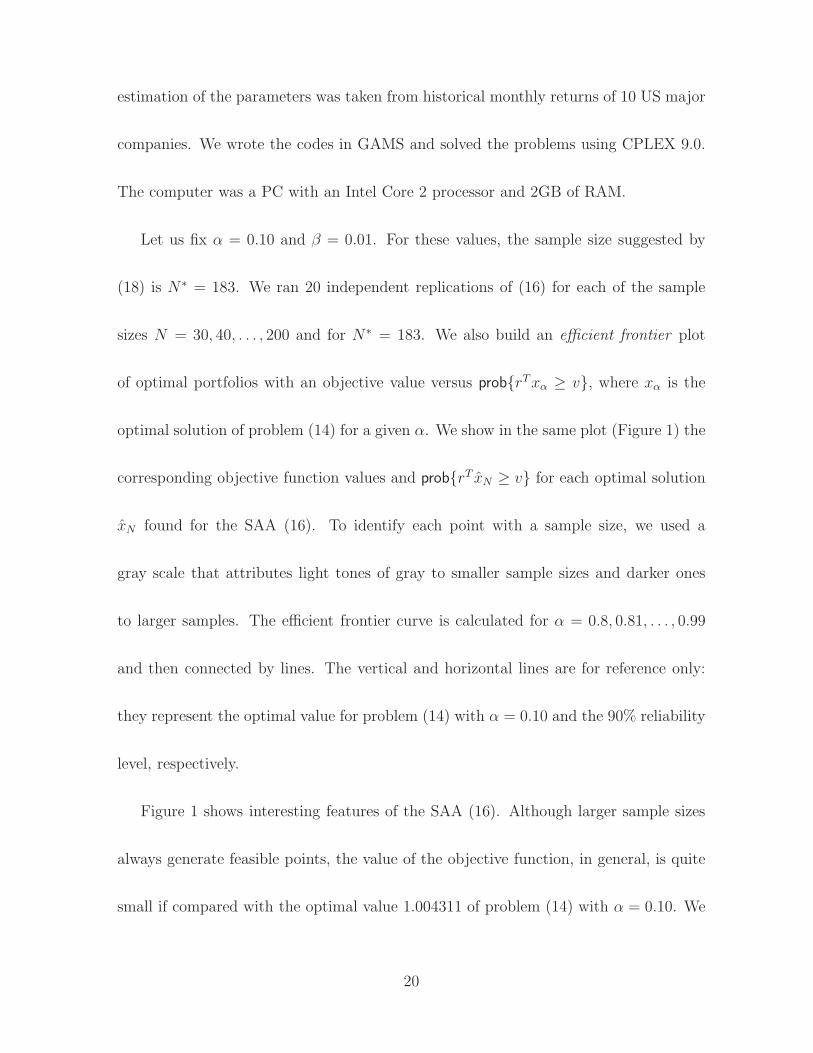
Let us fix α = 0.10 and β = 0.01. For these values, the sample size suggested by
(18) is N∗ = 183. We ran 20 independent replications of (16) for each of the sample
sizes N = 30, 40, . . . , 200 and for N∗ = 183. We also build an efficient frontier plot
of optimal portfolios with an objective value versus prob{rTxα ≥ v}, where xα is the
optimal solution of problem (14) for a given α. We show in the same plot (Figure 1) the
corresponding objective function values and prob{rT xN ≥ v} for each optimal solution
xN found for the SAA (16). To identify each point with a sample size, we used a
gray scale that attributes light tones of gray to smaller sample sizes and darker ones
to larger samples. The efficient frontier curve is calculated for α = 0.8, 0.81, . . . , 0.99
and then connected by lines. The vertical and horizontal lines are for reference only:
they represent the optimal value for problem (14) with α = 0.10 and the 90% reliability
level, respectively.
Figure 1 shows interesting features of the SAA (16). Although larger sample sizes
always generate feasible points, the value of the objective function, in general, is quite
small if compared with the optimal value 1.004311 of problem (14) with α = 0.10. We
20

also observe the absence of a convergence property: if we increase the sample size, the
feasible region of problem (16) gets smaller and the approximation becomes more and
more conservative and therefore suboptimal. The reason is that for increasingly large
samples the condition rTi x ≥ v for all i approaches the condition prob{rTx ≥ v} = 1.
We performed similar experiments for the lognormal case. For each point obtained
in the SAA, we estimated the probability by Monte-Carlo techniques. The reader is
referred to [20] for detailed instructions of how to generate samples from a multivariate
lognormal distribution. Since in the lognormal case one cannot compute the efficient
frontier, we also included in Figure 2 the upper bounds for α = 0.02, . . . , 0.20, calculated
according to (12). The detailed computation of the upper bounds will be given in the
next subsection.
In order to find better candidate solutions for problem (14), we need to solve the
SAA with γ > 0, (problem (19)), which is a combinatorial problem. Since our portfolio
problem is a linear one, we still can solve problem (15) efficiently for a moderate number
(e.g., 200 constraints) of instances. We performed tests for problem (15) with both
distributions, fixing γ = 0.05 and 0.10 and changing N .
The best candidate solutions to (14) were obtained with γ = 0.05. We considered
different sample sizes from 30 to 200. Although several points are infeasible to the
21

original problem, we observe in Figures 3 and 4 that whenever a point is feasible it is
close to optimal solution in the normal case or to the upper bound under lognormality.
For γ = 0.10, almost all generated points were infeasible in both cases, as seen in
Figures 5 and 6.
To investigate the different possible choices of γ and N in problem (19), we created
a three dimensional representation which we will call γN -plot. The domain is a dis-
cretization of values of γ and N , forming a grid with pairs (γ,N). For each pair we
solve an instance of problem (19) with these parameters and stored the optimal value
and the approximate probability of being feasible to the original problem (14). The
z-axis represents the optimal value associated to each point in the domain in the grid.
Finally, we created a surface of triangles based on this grid as follows. Let i be the
index for the values of γ and j for the values of N . If candidate points associated with
grid members (i, j), (i+ 1, j) and (i, j + 1) or (i+ 1, j + 1), (i+ 1, j) and (i, j + 1) are
feasible to problem (14) (with probability greater than or equal to (1 − α)), then we
draw a dark gray triangle connecting the three points in the space. Otherwise, we draw
a light gray triangle.
We created a γN -plot for problem (14) with normal returns. The result can be seen
in Figure 7, where we also included the plane corresponding to the optimal solution
22
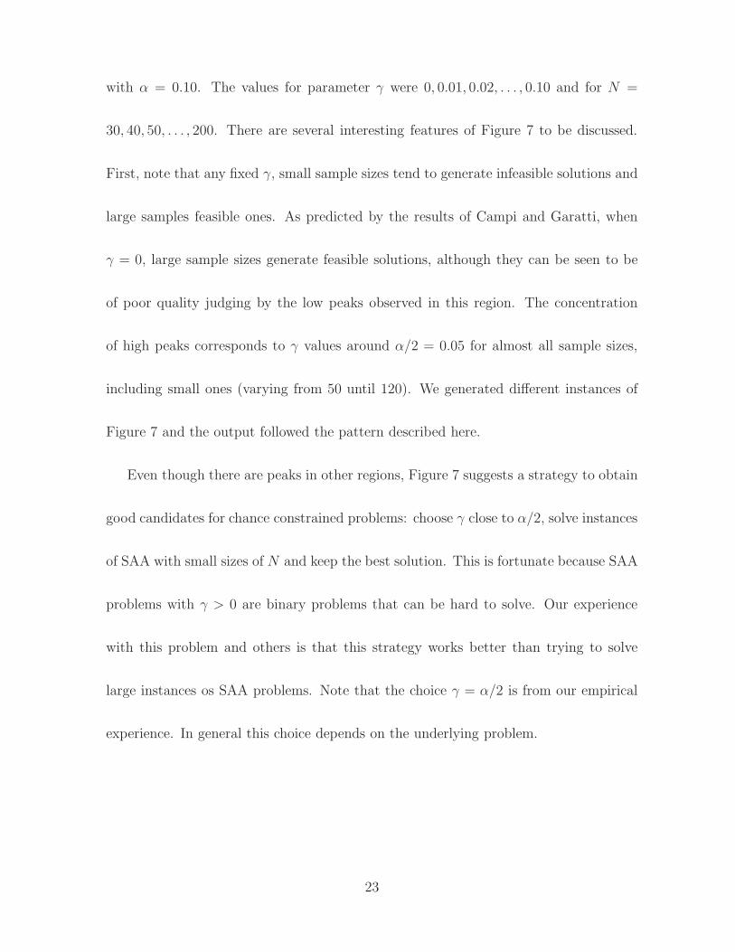
with α = 0.10. The values for parameter γ were 0, 0.01, 0.02, . . . , 0.10 and for N =
30, 40, 50, . . . , 200. There are several interesting features of Figure 7 to be discussed.
First, note that any fixed γ, small sample sizes tend to generate infeasible solutions and
large samples feasible ones. As predicted by the results of Campi and Garatti, when
γ = 0, large sample sizes generate feasible solutions, although they can be seen to be
of poor quality judging by the low peaks observed in this region. The concentration
of high peaks corresponds to γ values around α/2 = 0.05 for almost all sample sizes,
including small ones (varying from 50 until 120). We generated different instances of
Figure 7 and the output followed the pattern described here.
Even though there are peaks in other regions, Figure 7 suggests a strategy to obtain
good candidates for chance constrained problems: choose γ close to α/2, solve instances
of SAA with small sizes of N and keep the best solution. This is fortunate because SAA
problems with γ > 0 are binary problems that can be hard to solve. Our experience
with this problem and others is that this strategy works better than trying to solve
large instances os SAA problems. Note that the choice γ = α/2 is from our empirical
experience. In general this choice depends on the underlying problem.
23
3.3 Upper Bounds
A method to compute lower bounds of chance constrained problems of the form (1)
was suggested in [8]. We summarized that procedure at the end of Section 2 leaving
the question of how to choose the constants L,M and N . Given β,M and N , it is
straightforward to specify L: it is the largest integer that satisfies (12). For a given N ,
the larger M the better because we are approximating the L-th order statistic of the
random variable ϑN . However, note that M represents the number of problems to be
solved and this value is often constrained by computational limitations.
In [8] an indication of how N should be chosen is not given. It is possible to gain
some insight on the magnitude of N by doing some algebra in inequality (12). With
γ = 0, the first term (i = 0) of the sum (12) is
[
1 − (1 − α)N]M
≈[
1 − e−Nα]M
. (21)
Approximation (21) suggests that for small values of α we should take N of order
O(α−1). If N is much bigger than 1/α then we would have to choose a very large M in
order to honor inequality (12). For instance if α = 0.10, β = 0.01 and N = 100 instead
of N = 1/α = 10 or N = 2/α = 20, we need M to be greater than 100 000 in order to
24

satisfy (12), which can be computationally intractable for some problems. If N = 200
then M has to be grater then 109, which is impractical for most applications.
In [11], the authors applied the same technique to generate bounds on probabilistic
versions of the set cover problem and the transportation problem. To construct the
bounds they varied N and used M = 10 and L = 1. For many instances they obtained
lower bounds slightly smaller (less than 2%) or even equal to the best optimal values
generated by the SAA. In the portfolio problem, the choice L = 1 generated poor upper
bounds as we will see.
Since problem (14) is a maximization problem, we calculated upper bounds fixing
β = 0.01 for all cases and by choosing three different values for the constants L,M and
N . First we fixed L = 1 and N = ⌈1/α⌉ (solid line in Figure 2). The constant M was
chosen to satisfy the inequality (12). The results were not satisfactory, mainly because
M ended up being too small. Since the constant M defines the number of samples from
vN and since our problem is a linear one, we decided to fix M = 1 000. Then we chose
N = ⌈1/α⌉ (dashed line) and ⌈2/α⌉ (dotted line) in the next two experiments. The
constant L was chosen to be the largest integer such that (12) is satisfied. Figure 2
shows the generated points for the SAA with γ = 0 along with the upper bounds.
It is harder to construct upper bounds with γ > 0. The difficulty lies in an appro-
25

priate choice of the parameters since we cannot have very large values of M or N when
solving binary programs. Our experience shows that it is not significantly better than
the bounds obtained with γ = 0.
4 A Blending Problem
Let us consider a second example of chance constrained problems. Suppose a farmer
has some crop and wants to use fertilizers to increase the production. He hires an
agronomy engineer who recommends 7 g of nutrient A and 4 g of nutrient B. He has
two kinds of fertilizers available: the first has ω1 g of nutrient A and ω2 g of nutrient B
per kilogram. The second has 1 g of each nutrient per kilogram. The quantities ω1 and
ω2 are uncertain: we will assume they are (independent) continuous uniform random
variables with support in the intervals [1, 4] and [1/3, 1] respectively. Furthermore, each
fertilizer has a unitary cost per kilogram.
There are several ways to model this blending problem. A detailed discussion can
be found in [19], where the authors use this problem to motivate the field of stochastic
programming. We will consider a joint chance constrained formulation as follows:
minx1≥0,x2≥0
x1 + x2 s.t. prob{ω1x1 + x2 ≥ 7, ω2x1 + x2 ≥ 4} ≥ 1 − α, (22)
26
where xi represents the quantity of fertilizer i purchased, i = 1, 2, and α ∈ [0, 1] is the
reliability level. The independence assumption allows us to convert the joint probability
in (22) into a product of probabilities. After some calculations, one can explicitly solve
(22) for all values of α. For α ∈ [1/2, 1] the optimal solution and optimal value are
x∗1 =18
9 + 8(1 − α), x∗2 =
2(9 + 28(1 − α))
9 + 8(1 − α), v∗ =
4(9 + 14(1 − α))
9 + 8(1 − α).
For α ∈ [0, 1/2] we have
x∗1 =9
11 − 9(1 − α), x∗2 =
41 − 36(1 − α)
11 − 9(1 − α), v∗ =
2(25 − 18(1 − α))
11 − 9(1 − α). (23)
Our goal is to show that we can apply the SAA methodology to joint chance con-
strained problems. We can convert a joint chance constrained problem into a problem
of the form (1) using the min (or max) operators. Problem (22) becomes
minx1≥0,x2≥0
x1 + x2, s.t. prob {min{ω1x1 + x2 − 7, ω2x1 + x2 − 4} ≥ 0} ≥ 1 − α. (24)
27

It is possible to write the SAA of problem (24) as follows.
minx1≥0,x2≥0
x1 + x2, (25a)
s.t. ui ≤ ωi1x1 + x2 − 7, i = 1, . . . , N, (25b)
ui ≤ ωi2x1 + x2 − 4, i = 1, . . . , N, (25c)
ui +Kzi ≥ 0, i = 1, . . . , N, (25d)
N∑
i=1
zi ≤ Nγ, (25e)
zi ∈ {0, 1}N , (25f)
where N is the number of samples, ωi1 and ωi
2 are samples from ω1 and ω2, γ ∈ (0, 1)
and K is a positive constant positive constant greater or equal than 7.
4.1 Numerical Experiments
We performed experiments similar to the ones for the portfolio problem so we will
present the results without details. In Figure 8 we generated approximations for prob-
lem (22) with α = 0.05 using the SAA. The sample points were obtained by solving a
SAA with γ = 0.025 and sample sizes N = 60, 70, . . . , 150. The Campi-Garatti (18)
suggested value is N∗ = 130.We included the efficient frontier for problem (22). We will
28

not show the corresponding Figures for other values of γ, but the pattern observed in
the portfolio problem repeated: with γ = 0 almost every point was feasible but far from
the optimal, with γ = α = 0.05 almost every point was infeasible. The parameter choice
that generated the best candidate solutions was γ = α/2 = 0.025. We also show the
γN -plot for the SAA of problem (22). We tested γ values in the range 0, 0.005, . . . , 0.05
and N = 60, 70, . . . , 150. We included a plane representing the optimal value of problem
(22) for α = 0.05, which is readily obtained by applying formula (23).
In accordance with Figure 7, in Figure 9 the best candidate solutions are the ones
with γ around 0.025. Even for very small sample sizes we have feasible solutions (dark
gray triangles) close to the optimal plane. On the other hand, this experiment gives
more evidence that the SAA with γ = 0 is excellent to generate feasible solutions (dark
gray triangles) but the quality of the solutions is poor. As shown in Figure 9, the high
peaks associated with γ = 0 persist for any sample size, generating points far form the
optimal plane. In agreement with Figure 7, the candidates obtained for γ > α are in
their vast majority infeasible.
29

5 Conclusions
We have discussed chance constrained problems with a single constraint and proved
convergence results about the SAA method. We applied the SAA approach to a portfolio
chance constrained problem with random returns. In the normal case, we can compute
the efficient frontier and use it as a benchmark solution. Experiments show that the
sample size suggested by [17] was too conservative for our problem: a much smaller
sample can yield feasible solutions. We observed that the quality of the solutions
obtained was poor. Similar results were obtained for the lognormal case, where upper
bounds were computed using a method developed in [8].
As another illustration of the use of the SAA method, we presented a two dimen-
sional blending problem and modeled it as a joint chance constrained problem. We use
the problem as a benchmark to test the SAA approach and also to show how one can
use the SAA methodology to approximate joint chance constrained problems.
In both cases we observe that the choice γ = α/2 gave very good candidate solutions.
Even though it generated more infeasible points if compared to the choice γ = 0, the
feasible ones were of better quality. Using the γN -plot we were able to confirm these
empirical findings for our two test problems. Figures 7 and 9 tells us that relatively small
sample sizes (e.g, if compared to Campi-Garatti estimates) can yield good candidate
30
solutions. This is extremely important since for γ > 0 the SAA problem is an integer
program and large values ofN could quickly make the SAA approach intractable. Upper
bounds were also constructed for the portfolio problem using the SAA with γ = 0 by
solving several continuous linear programs. Since no closed solution is available for
the portfolio problem with lognormal returns, having an upper bound is an important
information about the variability of the solution.
We believe that the SAA methodology is suitable to approximate chance constrained
problems. Such problems are usually impossible to be solved explicitly and the pro-
posed method can yield good candidate solutions. One advantage of the method is
the fairly general assumption on the distribution of the random variables of the prob-
lem. One must only be able to sample from the given distribution in order to build
the corresponding SAA program. The main contribution of the paper is to present the
method and its theoretical foundations and to suggest parameter choices for the actual
implementation of the procedure.
31

References
1. Charnes, A., Cooper, W. W., Symmonds, G.H.: Cost horizons and certainty equiva-
lents: an approach to stochastic programming of heating oil. Manag. Sci. 4:235–263
(1958)
2. A. Prekopa.: Stochastic Programming. Kluwer Acad. Publ., Dordrecht, Boston
(1995)
3. Dupacova, J., Gaivoronski, A., Kos, Z., Szantai, T.: Stochastic programming in
water management: a case study and a comparison of solution techniques. Eur. J.
Oper. Res. 52:28–44 (1991)
4. Henrion, R., Li, P., Moller, A., Steinbach, S. G., Wendt, M., Wozny, G.: Stochastic
optimization for operating chemical processes under uncertainty. In Grtschel, M.,
Krunke, S., Rambau, J., (editors), Online optimization of large scale systems, pages
457–478, Springer (2001)
5. Henrion, R., Moller, A.: Optimization of a continuous distillation process under
random inflow rate. Comput. Math. Appl. 45:247–262 (2003)
6. Dentcheva, D., Prekopa, A., Ruszczynski, A.: Concavity and efficient points of dis-
crete distributions in probabilistic programming. Math. Program. 89:55–77 (2000)
32

7. Luedtke, J., Ahmed, S., Nemhauser, G.L.: An integer programming approach for
linear programs with probabilistic constraints. To appear in Math. Program (2007)
8. Nemirovski, A., Shapiro, A.: Convex approximations of chance constrained pro-
grams. SIAM J. on Optimiz. 17(4):969–996 (2006)
9. Shapiro, A.: Monte carlo sampling methods. In A. Ruszczynski and A. Shapiro,
editors, Stochastic Programming, volume 10 of Handbooks in OR & MS, pages
353–425. North-Holland Publishing Company (2003)
10. Atlason, J., Epelman, M.A., Henderson,S. G.: Optimizing call center staffing using
simulation and analytic center cutting plane methods. Manag. Sci. 54:295–309
(2008)
11. Luedtke, J., Ahmed, S.: A sample approximation approach for optimization with
probabilistic constraints. SIAM J. Optimiz. 19:674–699 (2008)
12. Rockafellar, R.T., Wets,R.J.-B.: Variational Analysis. Springer, Berlin (1998)
13. Artstein, Z., Wets, R.J.-B.: Consistency of minimizers and the slln for stochastic
programs. J. Convex Anal. 2:1–17 (1996)
14. Chernoff, H.: A measure of asymptotic efficiency for tests of a hypothesis based on
the sum observations. Annals Math. Stat. 23:493–507 (1952)
33

15. Markowitz, H.: Portfolio selection. J. Financ. 7:77–97 (1952)
16. Wang, Y., Chen, Z., Zhang, K.: A chance-constrained portfolio selection problem
under t-distrbution. Asia Pac. J. Oper. Res. 24(4):535–556 (2007)
17. Campi, M.C., Garatti, S.: The exact feasibility of randomized solutions of robust
convex programs. Optimization online (www.optimization-online.org) (2007)
18. Calafiore, G., Campi, M.C.: The scenario approach to robust control design. IEEE
T. Automat. Contr. 51:742–753 (2006)
19. Klein Haneveld, W.K., van der Vlerk, M.H.: Stochastic Programming (lecture
notes), (2007).
20. Law, A., Kelton, W.D.: Simulation Modeling and Analysis, Industrial Engineering
and Management Science Series. McGraw-Hill Science/Engineering/Math (1999).
34

0.998 1.004 1.010
0.80
0.85
0.90
0.95
1.00
Figure 1: Normal returns for γ = 0.
0.80
0.85
0.90
0.95
1.00
1.021.011.00
Figure 2: Lognormal returns, γ = 0.
0.80
0.85
0.90
0.95
1.00
0.998 1.004 1.010
Figure 3: Normal returns, γ = 0.05.
0.80
0.85
0.90
0.95
1.00
1.010 1.0301.020
Figure 4: Lognormal returns, γ = 0.05.
0.80
0.85
0.90
0.95
1.00
1.000 1.0101.0050.995
Figure 5: Normal returns, γ = 0.10.
0.80
0.85
0.90
0.95
1.00
1.005 1.010 1.015 1.020 1.025 1.030
Figure 6: Lognormal returns, γ = 0.10.
35

1.005
1.0
0.995
30 80 130 1800.0
0.025
0.05
0.075
0.1
1.01
Figure 7: γN -plot for the portfolio problem with normal returns.
0.90
0.95
1.00
6.05.5 7.06.5 7.5
Figure 8: Blending problem, γ = 0.025.
6.95
5.45
6.45
5.95
0.025
0.05
0.075
0.1
120
100
60
140
80
Figure 9: γN -plot (blending problem).
36