sample covariance matrices and high-dimensional data...

Sample covariance matrices and

high-dimensional data analysis

Jianfeng Yao

Shurong Zheng

Zhidong Bai

Contents

Notations page vi

Preface vii

1 Introduction 1

1.1 Large dimensional data and new asymptotic statistics 1

1.2 Random matrix theory 3

1.3 Eigenvalue statistics of large sample covariance matrices 4

1.4 Organisation of the book 5

2 Limiting spectral distributions 7

2.1 Introduction 7

2.2 Fundamental tools 8

2.3 Marcenko-Pastur distributions 10

2.4 Generalised Marcenko-Pastur distributions 16

2.5 LSD for random Fisher matrices 22

3 CLT for linear spectral statistics 30

3.1 Introduction 30

3.2 CLT for linear spectral statistics of a sample covariance matrix 31

3.3 Bai and Silverstein’s CLT 39

3.4 CLT for linear spectral statistics of random Fisher matrices 40

3.5 The substitution principle 44

4 The generalised variance and multiple correlation coefficient 47

4.1 Introduction 47

4.2 The generalised variance 47

4.3 The multiple correlation coefficient 52

5 The T 2-statistic 57

5.1 Introduction 57

5.2 Dempster’s non-exact test 58

5.3 Bai-Saranadasa’s test 60

5.4 Improvements of the Bai-Saranadasa test 62

5.5 Monte-Carlo results 66

6 Classification of data 69

6.1 Introduction 69

6.2 Classification into one of two known multivariate normal populations 69

iii

iv Contents

6.3 Classification into one of two multivariate normal populations

with unknown parameters 70

6.4 Classification into one of several multivariate normal populations 72

6.5 Classification under large dimensions: the T-rule and the D-rule 73

6.6 Misclassification rate of the D-rule in case of two normal populations 74

6.7 Misclassification rate of the T-rule in case of two normal populations 77

6.8 Comparison between the T-rule and the D-rule 78

6.9 Misclassification rate of the T-rule in case of two general populations 79

6.10 Misclassification rate of the D-rule in case of two general populations 83

6.11 Simulation study 89

6.12 A real data analysis 94

7 Testing the general linear hypothesis 97

7.1 Introduction 97

7.2 Estimators of parameters in multivariate linear regression 98

7.3 Likelihood ratio criteria for testing linear hypotheses about

regression coefficients 98

7.4 The distribution of the likelihood ratio criterion under the null 99

7.5 Testing equality of means of several normal distributions with

common covariance matrix 101

7.6 Large regression analysis 103

7.7 A large-dimensional multiple sample significance test 109

8 Testing independence of sets of variates 115

8.1 Introduction 115

8.2 The likelihood ratio criterion 115

8.3 The distribution of the likelihood ratio criterion under the null

hypothesis 118

8.4 The case of two sets of variates 120

8.5 Testing independence of two sets of many variates 122

8.6 Testing independence of more than two sets of many variates 126

9 Testing hypotheses of equality of covariance matrices 130


9.2 Criteria for testing equality of several covariance matrices 130

9.3 Criteria for testing that several normal distributions are identical 133

9.4 The sphericity test 136

9.5 Testing the hypothesis that a covariance matrix is equal to a given

matrix 138

9.6 Testing hypotheses of equality of large-dimensional covariance

matrices 139

9.7 Large-dimensional sphericity test 148

10 Estimation of the population spectral distribution 160


10.2 A method-of-moments estimator 161

10.3 An estimator using least sum of squares 166

10.4 A local moment estimator 176

Contents v

10.5 A cross-validation method for selection of the order of a popula-

tion spectral distribution 189

11 Large-dimensional spiked population models 201


11.2 Limits of spiked sample eigenvalues 203

11.3 Limits of spiked sample eigenvectors 209

11.4 Central limit theorem for spiked sample eigenvalues 211

11.5 Estimation of the values of spike eigenvalues 224

11.6 Estimation of the number of spike eigenvalues 226

11.7 Estimation of the noise variance 237

12 Efficient optimisation of a large financial portfolio 244


12.2 Mean-Variance Principle and the Markowitz’s enigma 244

12.3 The plug-in portfolio and over-prediction of return 247

12.4 Bootstrap enhancement to the plug-in portfolio 253

12.5 Spectrum-corrected estimators 257

Appendix A Curvilinear integrals 275

Appendix B Eigenvalue inequalities 282

Bibliography 285

Index 291

Notations

u, X, Σ etc. vectors and matrices are bold-faced

δ jk Kronecker symbol: 1/0 for j = k/ j , k

δa Dirac mass at a

e j j-th vector of a canonical basis

N(µ,Σ)multivariate Gaussian distribution with mean µ, covariance

matrix Σ and density function f (x|u,Σ)D= equality in distributionD−→ convergence in distributiona.s.−→ almost sure convergenceP−→ convergence in probability

oP(1), OP(1), oa.s(1), Oa.s.(1) stochastic order symbols

Γµ support set of a finite measure µ

ESD empirical spectral distribution

CLT central limit theorem

LSD limiting spectral distribution

PSD population spectral distribution

MP Marcenko-Pastur

I(·) indicator function

Ip p-dimensional identity matrix

vi

Preface

Dempster (1958, 1960) proposed a non-exact test for the two-sample significance test

when the dimension of data is larger than the degrees of freedom. He raised the question

that what statisticians should do if the traditional multivariate statistical theory does not

apply when the dimension of data is too large. Later, Bai and Saranadasa (1996) found that

even when the traditional approaches can be applied, they would be much less powerful

than the non-exact test when the dimension of data is large. This raised another question

that how could classical multivariate statistical procedures be adapted and improved when

the data dimension is large. These problems have attracted considerable attention since the

middle of the first decade of this century. Efforts towards the solution of these problems

have been made along two directions: the first is to propose special statistical procedures

to solve ad hoc large dimensional statistical problems where traditional multivariate sta-

tistical procedures are inapplicable or perform poorly, for some specific large-dimensional

hypotheses. The family of various non-exact tests follow this approach. The second di-

rection, following the work of Bai et al. (2009a), is to make systematic corrections to the

classical multivariate statistical procedures so that effect of large dimension is overcome.

This goal is achieved by employing new and powerful asymptotic tools borrowed from

the theory of random matrices such as the central limit theorems in Bai and Silverstein

(2004) and Zheng (2012).

Recently, research along these two directions becomes very active in response to an

increasingly important need for analysis of massive and large dimensional data. Indeed,

such “big data” is nowadays routinely collected due to the rapid advances in computer-

based or web-based commerce and data-collection technology.

To accommodate such need, this monograph is prepared by collecting some existing

results along the aforementioned second direction of large dimensional data analysis. In

a first part, the core of fundamental results from the random matrix theory about sam-

ple covariance matrices and random Fisher matrices is presented in details. The second

part of the book is made with a collection of large dimensional statistical problems where

the classical large sample methods fail and the new asymptotic methods, based on the

fundamental results of the first part, provide a valuable remedy. As the employed statis-

tical and mathematical tools are quite new and technically demanding, our objective is

to give a state-of-the-art though accessible introduction to these new statistical tools. It

is assumed that the reader is familiar with the usual theory of mathematical statistics, es-

pecially methods dealing with multivariate normal samples. Other prerequisites include

knowledge of elementary matrix algebra, limit theory (law of large number and central

vii

viii Preface

limit theorem) for independent and identically distributed samples. A special prerequisite

is some familiarity with contour integration; however, a detailed appendix on this topic

has been included.

Reader familiar with the textbook An Introduction to Multivariate Statistical Analy-

sis (Anderson, 2003) will easily recognise that our introduction to classical multivariate

statistical methods such as in Chapters 4, 7,8 and 9 follow closely this textbook. We are

deeply grateful to this phenomenal text that has been of constant help during the prepara-

tion of this book.

This text has also benefited over the years from numerous collaborations with our col-

leagues and research students. We particularly thank the following individuals whose joint

research work with us has greatly contributed to the material presented in the book: Ji-

aqi Chen, Bernard Delyon, Xue Ding, Dandan Jiang, Weiming Li, Zhaoyuan Li, Hua Li,

Huixia Liu, Guangming Pan, Damien Passemier, Yingli Qin, Hewa Saranadasa, Jack Sil-

verstein, Qinwen Wang and Wing-Keung Wong.

Finally, two of us owe a debt of gratitude to Zhidong Bai: he has been for years a con-

stant inspiration to us. This text would never have been possible without his outstanding

leadership. We are particularly proud of the completion of the text on the year of his 70th

birthday.

Jianfeng Yao

Shurong Zheng

Zhidong Bai

Changchun and Hong Kong

April, 2014

1

Introduction

1.1 Large dimensional data and new asymptotic statistics

In a multivariate analysis problem, we are given a sample x1, x2, . . . , xn of random ob-

servations of dimension p. Statistical methods such as Principal Components Analysis

have been developed since the beginning of the 20th century. When the observations are

Gaussian, some nonasymptotic methods exist such as Student’s test, Fisher’s test or the

analysis of variance. However in most of applications, observations are non Gaussian at

least in part so that nonasymptotic results become hard to obtain and statistical methods

are built using limiting theorems on model statistics.

Most of these asymptotic results are derived under the assumption that the data dimen-

sion p is fixed while the sample size n tends to infinity (large sample theory). This theory

has been adopted by most of practitioner until very recently when they are faced with a

new challenge, the analysis of large dimensional data.

Large dimensional data appear in various fields due to different reasons. In finance, as

a consequence of the generalisation of Internet and electronic commerce supported by

an exponentially increasing power of computing, on-line data from markets around the

world are accumulated in a giga-octets basis every day. In genetic experiments such as

micro-arrays, it becomes possible to record the expression of several thousands of genes

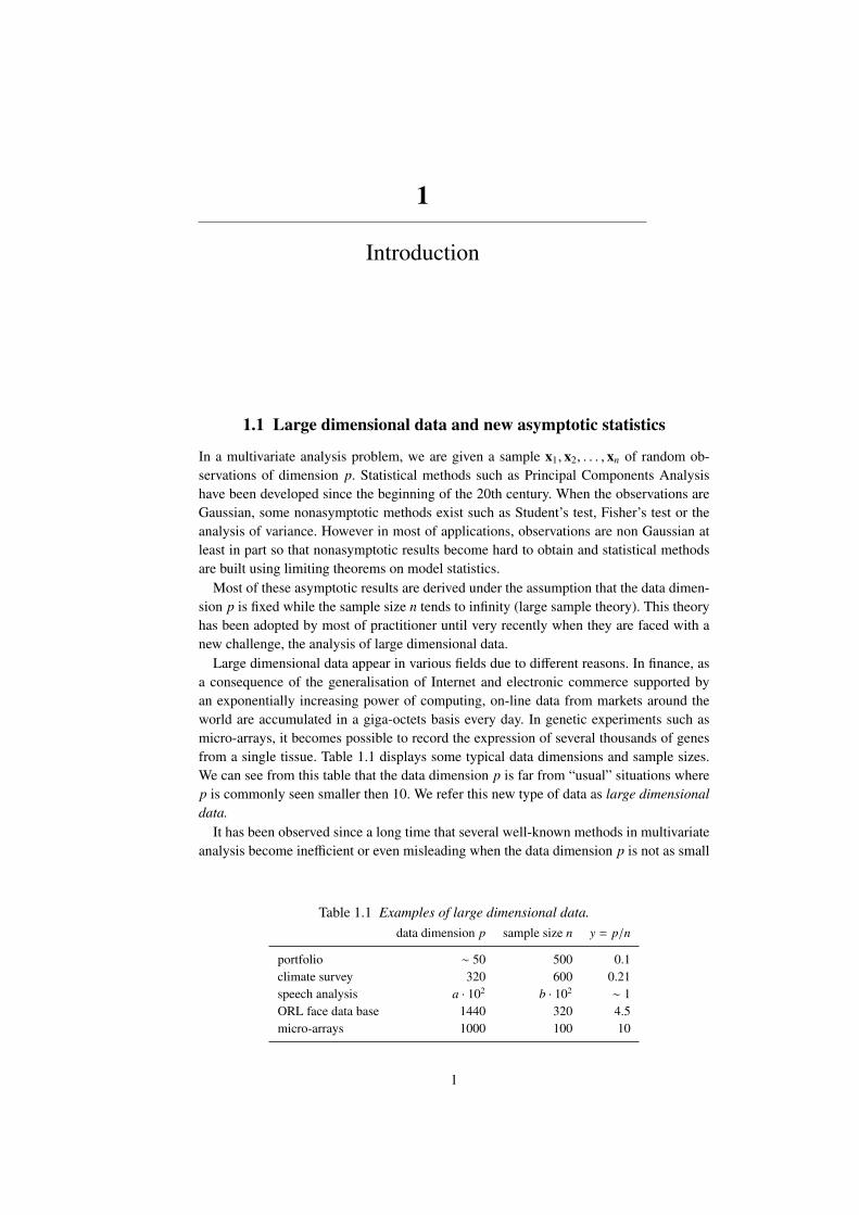
from a single tissue. Table 1.1 displays some typical data dimensions and sample sizes.

We can see from this table that the data dimension p is far from “usual” situations where

p is commonly seen smaller then 10. We refer this new type of data as large dimensional

data.

It has been observed since a long time that several well-known methods in multivariate

analysis become inefficient or even misleading when the data dimension p is not as small

Table 1.1 Examples of large dimensional data.

data dimension p sample size n y = p/n

portfolio ∼ 50 500 0.1

climate survey 320 600 0.21

speech analysis a · 102 b · 102 ∼ 1

ORL face data base 1440 320 4.5

micro-arrays 1000 100 10

1

2 Introduction

as say several tens. A seminar example is provided by Dempster in 1958 where he estab-

lished the inefficiency of Hotellings’ T 2 in such cases and provided a remedy (named as a

non-exact test). However, by that time no statistician was able to discover the fundamental

reasons for such break-down of the well-established methods.

To deal with such large-dimensional data, a new area in asymptotic statistics has been

developed where the data dimension p is no more fixed but tends to infinity together with

the sample size n. We call this scheme large dimensional asymptotics. For multivariate

analysis, the problem thus turns out to be which one of the large sample scheme and the

large dimensional scheme is closer to reality? As argued in Huber (1973), some statis-

ticians might say that five samples for each parameter in average are enough for using

large sample asymptotic results. Now, suppose there are p = 20 parameters and we have

a sample of size n = 100. We may consider the case as p = 20 being fixed and n tending

to infinity (large sample asymptotics), p = 2√

n or p = 0.2n (large dimensional asymp-

totics). So, we have at least three different options to choose for an asymptotic setup. A

natural question is then, which setup is the best choice among the three? Huber strongly

suggested to study the situation of increasing dimension together with the sample size in

linear regression analysis.

This situation occurs in many cases. In parameter estimation for a structured covari-

ance matrix, simulation results show that parameter estimation becomes very poor when

the number of parameters is more than four. Also, it is found that in linear regression

analysis, if the covariates are random (or having measurement errors) and the number of

covariates is larger than six, the behaviour of the estimates departs far away from the theo-

retical values, unless the sample size is very large. In signal processing, when the number

of signals is two or three and the number of sensors is more than 10, the traditional MU-

SIC (MUltivariate SIgnal Classification) approach provides very poor estimation of the

number of signals, unless the sample size is larger than 1000. Paradoxically, if we use

only half of the data set, namely, we use the data set collected by only five sensors, the

signal number estimation is almost hundred-percent correct if the sample size is larger

than 200. Why would this paradox happen? Now, if the number of sensors (the dimension

of data) is p, then one has to estimate p2 parameters ( 12

p(p + 1) real parts and 12

p(p − 1)

imaginary parts of the covariance matrix). Therefore, when p increases, the number of

parameters to be estimated increases proportional to p2 while the number (2np) of ob-

servations increases proportional to p. This is the underlying reason of this paradox. This

suggests that one has to revise the traditional MUSIC method if the sensor number is

large.

An interesting problem was discussed by Bai and Saranadasa (1996) who theoretically

proved that when testing the difference of means of two high dimensional populations,

Dempster (1958) non-exact test is more powerful than Hotelling’s T 2 test even when

the T 2-statistic is well defined. It is well known that statistical efficiency will be signifi-

cantly reduced when the dimension of data or number of parameters becomes large. Thus,

several techniques of dimension reduction were developed in multivariate statistical anal-

ysis. As an example, let us consider a problem in principal component analysis. If the

data dimension is 10, one may select 3 principal components so that more than 80% of

the information is reserved in the principal components. However, if the data dimension

is 1000 and 300 principal components are selected, one would still have to face a large

dimensional problem. If again 3 principal components only are selected, 90% or even

1.2 Random matrix theory 3

more of the information carried in the original data set could be lost. Now, let us consider

another example.

Example 1.1 Let x1, x2, . . . , xn be a sample from p-dimensional Gaussian distribution

Np(0, Ip) with mean zero and unit covariance matrix. The corresponding sample covari-

ance matrix is

Sn =1

n

n∑

i=1

xix∗i .

An important statistic in multivariate analysis is

Tn = log(det Sn) =

p∑

j=1

log λn, j,

where {λn, j}1≤ j≤p are the eigenvalues of Sn. When p is fixed, λn, j→1 almost surely as

n→∞ and thus Tn→0. Further, by taking a Taylor expansion of log(1 + x), one can show

that √n

pTn

D−→ N(0, 2),

for any fixed p. This suggests the possibility that Tn remains asymptotically Gaussian for

large p provided that p = O(n). However, this is not the case. Let us see what happens

when p/n→y∈(0, 1) as n→∞. Using results on the limiting spectral distribution of Sn [see

Chapter 2], it is readily seen that almost surely,

1

pTn→

∫ b(y)

a(y)

log x

2πyx

[{b(y) − x}{x − a(y)}]1/2dx =

y − 1

ylog(1 − y) − 1 ≡ d(y) < 0 ,

where a(y) = (1 − √y)2 and b(y) = (1 +√

y)2 (details of this calculation of integral are

given in Example 2.11). This shows that almost surely√

n

pTn ≃ d(y)

√np→−∞.

Thus, any test which assumes asymptotic normality of Tn will result in a serious error.

These examples show that the classical large sample limits are no longer suitable for

dealing with large dimensional data analysis. Statisticians must seek out new limiting

theorems to deal with large dimensional statistical problems. In this context, the theory of

random matrices (RMT) proves to be a powerful tool for achieving this goal.

1.2 Random matrix theory

RMT traces back to the development of quantum mechanics in the 1940s and the early

1950s. In this field, the energy levels of a system are described by eigenvalues of a Her-

mitian operator A on a Hilbert space, called the Hamiltonian. To avoid working with an

infinite dimensional operator, it is common to approximate the system by discretisation,

amounting to a truncation, keeping only the part of the Hilbert space that is important to

the problem under consideration. Thus A becomes a finite but large dimensional random

linear operator, i.e. a large dimensional random matrix. Hence, the limiting behaviour

4 Introduction

of large dimensional random matrices attracts special interest among experts in quantum

mechanics and many limiting laws were discovered during that time. For a more detailed

review on applications of RMT in quantum mechanics and other related areas in physics,

the reader is referred to the Book Random Matrices by Mehta (2004).

Since the late 1950s, research on the limiting spectral properties of large dimensional

random matrices has attracted considerable interest among mathematicians, probabilists

and statisticians. One pioneering work is the semicircular law for a Gaussian (or Wigner)

matrix , due to E. Wigner (1955; 1958). He proved that the expected spectral distribu-

tion of a large dimensional Wigner matrix tends to the semicircular law. This work was

later generalised by Arnold (1967, 1971) and Grenander (1963) in various aspects. On

the another direction related to the class of Gaussian Wishart matrices, or more generally,

the class of sample covariance matrices, the breakthrough work was done in Marcenko

and Pastur (1967) and Pastur (1972, 1973) where the authors discovered the Marcenko-

Pastur law under fairly general conditions. The asymptotic theory of spectral analysis of

large dimensional sample covariance matrices was later developed by many researchers

including Bai et al. (1986), Grenander and Silverstein (1977), Jonsson (1982), Wachter

(1978), Yin (1986), and Yin and Krishnaiah (1983). Also, Bai et al. (1986, 1987), Sil-

verstein (1985), Wachter (1980), Yin (1986), and Yin and Krishnaiah (1983) investigated

the limiting spectral distribution of the multivariate Fisher matrix, or more generally, of

products of random matrices (a random Fisher matrix is the product of a sample covari-

ance matrix by the inverse of another independent sample covariance matrix). In the early

1980s, major contributions on the existence of limiting spectral distributions and their

explicit forms for certain classes of random matrices were made. In particular, Bai and

Yin (1988) proved that the spectral distribution of a sample covariance matrix (suitably

normalised) tends to the semicircular law when the dimension is relatively smaller than

the sample size. In recent years, research on RMT is turning toward the second order lim-

iting theorems, such as the central limit theorem for linear spectral statistics, the limiting

distributions of spectral spacings and extreme eigenvalues.

1.3 Eigenvalue statistics of large sample covariance matrices

This book is about the theory of large sample covariance matrices and their applications

to high-dimensional statistics. Let x1, x2, . . . , xn be a sample of random observations of

dimension p. The population covariance matrix is denoted by Σ = cov(xi). The corre-

sponding sample covariance matrix is defined as

Sn =1

n − 1

n∑

i=1

(xi − x)(xi − x)∗, (1.1)

where x = n−1∑

i xi denotes the sample mean. Almost all statistical methods in multivari-

ate analysis rely on this sample covariance matrix: principle component analysis, canon-

ical correlation analysis, multivariate regressions, one-sample or two-sample hypothesis

testing, factor analysis etc.

A striking fact in multivariate analysis or large dimensional statistics is that many im-

portant statistics are function of the eigenvalues of sample covariance matrices. The statis-

tic Tn in Example 1.1 is of this type and here is yet another example.

1.4 Organisation of the book 5

Example 1.2 Let the covariance matrix of a population have the form Σ = Σq + σ2I,

where Σ is p × p and Σq has rank q (q < p). Suppose Sn is the sample covariance matrix

based on a sample of size n drawn from the population. Denote the eigenvalues of Sn by

λ1 ≥ λ2 ≥ · · · ≥ λp. Then the test statistic for the hypothesis H0: rank(Σq) = q against H1:

rank(Σq) > q is given by

Qn =1

p − q

p∑

j=q+1

λ2j −

1

p − q

p∑

j=q+1

λ j

2

.

In other words, the test statistic Qn is the variance of the p− q smallest eigenvalues of Sn.

Therefore, understanding the asymptotic properties of eigenvalue statistics such as Tn

and Qn above has a paramount importance in data analysis when the dimension p is

getting large with respect to the sample size. The spectral analysis of large dimensional

sample covariance matrices from RMT provides powerful tools for the study of such

eigenvalue statistics. For instance, the Marcenko-Pastur law describe the global behaviour

of the p eigenvalues of a sample covariance matrix so that point-wise limits of eigen-

value statistics are determined by integrals of appropriate functions with respect to the

Marcenko-Pastur law, see Example 1.1 for the case of Tn. Moreover, fluctuations of these

eigenvalue statistics are described by central limit theorems which are found in Bai and

Silverstein (2004) and in Zheng (2012). Similarly to the case of classical large sample the-

ory, such CLTs constitute the corner-stones of statistical inference with large dimensional

data.

1.4 Organisation of the book

The book has a quite simple structure. In a first part, the core of fundamental results from

RMT regarding sample covariance matrices and random Fisher matrices is presented in

details. These results are selected in such a way that they are applied and used in the

subsequent chapters of the book. More specifically, Chapter 2 introduces the limiting

spectral distributions of general sample covariance matrices, namely the Marcenko-Pastur

distributions, and the limiting spectral distributions of random Fisher matrices. Detailed

examples of both limits are also provided. In Chapter 3, the two fundamental CLTs from

Bai and Silverstein (2004) and Zheng (2012) are presented in details. Simple application

examples of these CLTs are given. We also introduce a substitution principle that deals

with the effect in the CLTs induced by the use of adjusted sample sizes ni − 1 in place

of the (raw) sample sizes ni in the definition of sample covariance matrices and Fisher

matrices.

The second and longer part of the book is made with a collection of large dimensional

statistical problems where the classical large sample methods fail and the new asymptotic

methods from the above RMT provide a valuable remedy. The problems run from the

“simple” and classical two-sample test problem (Chapter 5) to the current and advanced

topic of the Markowitz portfolio optimisation problem (Chapter 12). Topics from Chap-

ter 4 to Chapter 9 are classical topics in multivariate analysis; they are here re-analysed

under the large-dimensional scheme. The last three chapters cover three modern topics in

6 Introduction

large-dimensional statistics. Methods and results reported there have been so far available

in research papers only.

A characteristic feature of the book is that the nine chapters of the second part are quite

independent each other so that they can be read in an arbitrary order once the material in

the first part is understood. Notice however dependence between some of these chapters

might exist occasionally but this remains very limited.

Finally, we have included an appendix to introduce the basics on contour integration.

The reason is that in the CLT’s developed in Chapter 3 for linear spectral statistics of sam-

ple covariance matrices and of random Fisher matrices, the mean and covariance func-

tions of the limiting Gaussian distributions are expressed in terms of contour integrals,

and explicit calculations of such contour integrals frequently appear in various chapters

of this book. As such calculations are not always taught in non-mathematical curricula, it

is hoped that such an appendix will help the reader to follow some basic calculations in

the use of aforementioned CLT’s.

Notes

On the interplay between the random matrix theory and large-dimensional statistics, sup-

plementary information can be found in the excellent introductory papers Bai (2005)

Johnstone (2007) and Johnstone and Titterington (2009).

2

Limiting spectral distributions

2.1 Introduction

Let x1, x2, . . . , xn be a sample of random observations of dimension p. The sample covari-

ance matrix is defined as

Sn =1

n − 1

n∑

i=1

(xi − x)(xi − x)∗ =1

n − 1

n∑

i=1

xix∗i −

n

n − 1xx∗, (2.1)

where x = n−1∑

i xi denotes the sample mean. Many of traditional multivariate statistics

are functions of the eigenvalues {λk} of the sample covariance matrix Sn. In the most basic

form, such statistics can be written as

Tn =1

p

p∑

k=1

ϕ(λk) , (2.2)

for some specific function ϕ. Such statistic is called a linear spectral statistic of the sample

covariance matrix Sn. For example, the so-called generalised variance discussed later in

Chapter 4, see Eq.(4.1) is

Tn =1

plog |Sn| =

1

p

p∑

k=1

log(λk).

So this particular Tn is a linear spectral statistic of the sample covariance matrix Sn with

“test function” ϕ(x) = log(x).

In two-sample multivariate analysis with say an x-sample and an y-sample, interesting

statistics will still be of the previous form in (2.2), where however the eigenvalues {λk}will be those of the so-called Fisher matrix Fn. Notice that each of the two examples has

a corresponding sample covariance matrix, say Sx and Sy. The Fisher matrix associated to

these samples is the quotient of the two sample matrices, namely Fn = SxS−1y (assuming

the later is invertible).

Linear spectral statistics of sample covariance matrices or Fisher matrices are at the

heart of the new statistical tools developed in this book. In this chapter and the next Chap-

ter 3, we introduce the theoretical backgrounds on these statistics. More specifically, this

chapter deals with the first order limits of such statistics, namely to answer the question:

When and how Tn should converge to some limiting value ℓ as both the dimension p and the sample

size grow to infinity?

7

8 Limiting spectral distributions

Clearly, the question should relate to the “joint limit” of the p eigenvalues {λk}. The formal

concepts to deal with the question are called the empirical spectral distributions and lim-

iting spectral distributions. In this chapter, these distributions for the sample covariance

matrix Sn and the two-sample Fisher matrix Fn are introduced.

2.2 Fundamental tools

This section introduces some fundamental concepts and tools used throughout the book.

2.2.1 Empirical and limiting spectral distributions

Let Mp(C) be the set of p × p matrices with complex-valued elements.

Definition 2.1 Let A ∈ Mp(C) and {λ j}1≤ j≤p, its empirical spectral distribution (ESD)

is

FA =1

p

p∑

j=1

δλ j,

where δa denotes the Dirac mass at a point a.

In general, the ESD FA is a probability measure onC; it has support inR (resp. onR+) if

A is Hermitian (resp. nonnegative definite Hermitian). For example, the two-dimensional

rotation

A =

(0 −1

1 0

)

has eigenvalues ±i so that FA = 12(δ{i} + δ{−i}) is a measure on C, while the symmetry

B =

(0 1

1 0

)

has eigenvalues ±1 so that FB = 12(δ{1} + δ{−1}) has support on R. In this book, we are

mainly concerned by covariance matrices. Since there are Hermitian and nonnegative

definite, the corresponding ESD’s will have support on R+.

Definition 2.2 Let {An}n≥1 be a sequence from Mp(C). If the sequence of corresponding

ESD’s {FAn }n≥1 vaguely converges to a (possibly defective) measure F, we call F the

limiting spectral distribution (LSD) of the sequence of matrices {An}.

The above vague convergence means that for any continuous and compactly supported

function ϕ, FAn (ϕ) → F(ϕ) as n → ∞. It is well-known that if the LSD F is indeed non

defective, i.e.∫

F(dx) = 1, the above vague convergence turns into the stronger (usual)

weak convergence, i.e. FAn (ϕ)→ F(ϕ) for any continuous and bounded function ϕ.

When dealing with a sequence of sample covariance matrices {Sn}, their eigenvalues are

random variables and the corresponding ESD’s {FSn } are random probability measures on

R+. A fundamental question in random matrix theory is about whether the sequence {FSn }has a limit (in probability or almost surely).

2.2 Fundamental tools 9

2.2.2 Stieltjes transform

The eigenvalues of a matrix are continuous functions of entries of the matrix. But these

functions have no closed forms when the dimension of the matrix is larger than four. So

special methods are needed for their study. There are three important methods employed

in this area, moment method, Stieltjes transform and orthogonal polynomial decomposi-

tion of the exact density of eigenvalues. For the sake of our exposition, we concentrate

on the Stieltjes transform method which is indeed widely used in the literature of large

dimensional statistics.

We denote by Γµ the support of a finite measure µ on R. Let

C+ :=

{z ∈ C : ℑ(z) > 0

}

be the (open) upper half complex plan with positive imaginary part.

Definition 2.3 Let µ be a finite measure on the real line. Its Stieltjes transform (also

called Cauchy transform in the literature) is defined as

sµ(z) =

∫1

x − zµ(dx) , z ∈ C \ Γµ .

The results of this section are given without proofs; they can be found in textbooks such

as Kreın and Nudel′man (1977).

Proposition 2.4 The Stieltjes transform has the following properties:

(i) sµ is holomorphic on C \ Γµ;

(ii) z ∈ C+ if and only if sµ(z) ∈ C+ ;

(iii) If Γµ ⊂ R+ and z ∈ C+, then zsµ(z) ∈ C+;

(iv) |sµ(z)| ≤ µ(1)

dist(z,Γµ) ∨ |ℑ(z)| .

The next result is an inversion result.

Proposition 2.5 The mass µ(1) can be recovered through the formula

µ(1) = limv→∞−ivsµ(iv) .

Moreover, for all continuous and compactly supported ϕ: R→ R,

µ(ϕ) =

∫

R

ϕ(x)µ(dx) = limv↓0

1

π

∫

R

ϕ(x)ℑsµ(x + iv)dx .

In particular, for two continuity points a < b of µ,

µ([a, b]) = limv↓0

1

π

∫ b

a

ℑsµ(x + iv)dx .

The next proposition characterises functions that are Stieltjes transforms of bounded

measures on R.

Proposition 2.6 Assume that the following conditions hold for a complex valued func-

tion g(z):

(i) g is holomorphic on C+;

(ii) g(z) ∈ C+ for all z ∈ C+;


(iii) lim supv→∞

|ivg(iv)| < ∞.

Then g is the Stieltjes transform of a bounded measure on R.

Similar to the characterisation of the weak convergence of finite measures by the con-

vergence of their Fourier transforms, Stieltjes transform characterises the vague conver-

gence of finite measures. This a key tool for the study of the ESD’s of random matrices.

Theorem 2.7 A sequence {µn} of probability measures on R converges vaguely to some

positive measure µ (possibly defective) if and only if their Stieltjes transforms {sµn} con-

verges to sµ on C+.

In order to get the weak convergence of {µn}, one checks the vague convergence of the

sequence using this theorem and then to ensure that the limiting measure µ is a probability

measure, i.e. to check µ(1) = 1 through Proposition 2.5 or by some direct observation.

The Stieltjes transform and the RMT are closely related each other. Indeed, the Stieltjes

transform of the ESD FA of a n × n Hermitian matrix A is by definition

sA(z) =

∫1

x − zFA(dx) =

1

ntr(A − zI)−1 , (2.3)

which is the resolvent of the matrix A (up to the factor 1/n). Using a formula for the trace

of an inverse matrix, see Bai and Silverstein (2010, Theorem A.4), we have

sn(z) =1

n

n∑

k=1

1

akk − z − α∗k(Ak − zI)−1αk

, (2.4)

where Ak is the (n − 1) × (n − 1) matrix obtained from A with the k-th row and column

removed and αk is the k-th column vector of A with the k-th element removed. If the

denominator akk − z − α∗k(Ak − zI)−1αk can be proved to be equal to g(z, sn(z)) + o(1) for

some function g, then a LSD F exists and its Stieltjes transform is the solution to the

equation

s = 1/g(z, s).

Its applications will be discussed in more detail later in the chapter.

2.3 Marcenko-Pastur distributions

The Marcenko-Pastur distribution Fy,σ2 (M-P law) with index y and scale parameter σ

has the density function

py,σ2 (x) =

1

2πxyσ2

√(b − x)(x − a), if a ≤ x ≤ b,

0, otherwise,(2.5)

with an additional point mass of value 1−1/y at the origin if y > 1, where a = σ2(1− √y)2

and b = σ2(1 +√

y)2. Here, the constant y is the dimension to sample size ratio index

and σ2 the scale parameter. The distribution has mean σ2 and variance yσ4. The support

interval has a length of b − a = 4σ2 √y.

If σ2 = 1, the distribution is said to be a standard M-P distribution (then we simplify

the notations to Fy and py for the distribution and its density function). Three standard


M-P density functions for y ∈ { 18, 1

4, 1

2} are displayed on Figure 2.1. In particular, the

density function behaves as√

x − a and√

b − x at the boundaries a and b, respectively.

Figure 2.1 Density plots of the Marcenko-Pastur distributions with indexes y = 1/8 (dashed

line), 1/4 (dotted line) and 1/2 (solid line).

Example 2.8 For the special case of y = 1, the density function is

p1(x) =

{1

2πx

√x(4 − x), if 0 < x ≤ 4,

0, otherwise.(2.6)

In particular, the density is unbounded at the origin.

It is easy to see that when the index y tends to zero, the M-P law Fy shrinks to the

Dirac mass δ1. More intriguing is the following fact (that can be easily checked though):

if Xy follows the M-P distribution Fy, then as y → 0, the sequence 12√

y(Xy − 1) weakly

converges to Wigner’s semi-circle law with density function π−1√

1 − x2 for |x| ≤ 1.

2.3.1 The M-P law for independent vectors without cross-correlations

Notice first that regarding limiting spectral distributions discussed in this chapter, one may

ignore the rank-1 matrix xx∗

in the definition of the sample covariance matrix and define

the sample covariance matrix to be

Sn =1

n

n∑

i=1

xix∗i . (2.7)

Indeed, by Weilandt-Hoffman inequality, the eigenvalues of the two forms of sample co-

variance matrix are interlaced each other so that they have a same LSD (when it exists).

As a notational ease, it is also convenient to summarise the n sample vectors into a p×n

random data matrix X = (x1, . . . , xn) so that Sn =1nXX∗.

Marcenko and Pastur (1967) first finds the LSD of the large sample covariance matrix

Sn. Their result has been extended in various directions afterwards.


Theorem 2.9 Suppose that the entries {xi j} of the data matrix X are i.i.d. complex ran-

dom variables with mean zero and variance σ2, and p/n → y ∈ (0,∞). Then almost

surely, FSn weakly converges to the MP law Fy,σ2 (2.5).

This theorem was found as early as in the late sixties (convergence in expectation).

However its importance for large-dimensional statistics has been recognised only recently

at the beginning of this century. To understand its deep influence on multivariate analysis,

we plot in Figure 2.2 sample eigenvalues from i.i.d. Gaussian variables {xi j}. In other

words, we use n = 320 i.i.d. random vectors {xi}, each with p = 40 i.i.d. standard Gaussian

coordinates. The histogram of p = 40 sample eigenvalues of Sn displays a wide dispersion

from the unit value 1. According to the classical large-sample asymptotic (assuming n =

320 is large enough), the sample covariance matrix Sn should be close to the population

covariance matrix Σ = Ip = E xix∗i. As eigenvalues are continuous functions of matrix

entries, the sample eigenvalues of Sn should converge to 1 (unique eigenvalue of Ip). The

plot clearly assesses that this convergence is far from the reality. On the same graph is also

plotted the Marcenko-Pastur density function py with y = 40/320 = 1/8. The closeness

between this density and the sample histogram is striking.

Figure 2.2 Eigenvalues of a sample covariance matrix with standard Gaussian entries, p = 40

and n = 320. The dashed curve plots the M-P density py with y = 1/8 and the vertical bar

shows the unique population unit eigenvalue.

Since the sample eigenvalues deviate significantly from the population eigenvalues, the

sample covariance matrix Sn is no more a reliable estimator of its population counter-part

Σ. This observation is indeed the fundamental reason for that classical multivariate meth-

ods break down when the data dimension is a bit large compared to the sample size. As an

example, consider Hotelling’s T 2 statistic which relies on S−1n . In large-dimensional con-

text (as p = 40 and n = 320 above), S−1n deviates significantly from Σ−1. In particular, the

wider spread of the sample eigenvalues implies that Sn may have many small eigenvalues,

especially when p/n is close to 1. For example, for Σ = σ2Ip and y = 1/8, the smallest

eigenvalue of Sn is close to a = (1 − √y)2σ2 = 0.42σ2 so that the largest eigenvalue of

S−1n is close to a−1σ−2 = 1.55σ−2, a 55% over-spread to the population value σ−2. When


the data to sample size increases to y = 0.9, the largest eigenvalue of S−1n becomes close

to 380σ−2! Clearly, S−1n is completely unreliable as an estimator of Σ−1.

2.3.2 How the Marcenko-Pastur law appears in the limit?

As said in Introduction, most of results in RMT require advanced mathematical tools

which are exposed in details elsewhere. Here an explanation why the LSD should be the

Marcenko-Pastur distribution is given using Stieltjes transform.

Throughout this book, for a complex number z (or a negative real number),√

z denotes

its square root with positive imaginary part. Without loss of generality, the scale parameter

is fixed to σ2 = 1. Let z = u + iv with v > 0 and s(z) be the Stieltjes transform of the M-P

distribution Fy. From the definition of the density function py in (2.5), it is not difficult to

find that the Stieltjes transform of the M-P distribution Fy equals

s(z) =(1 − y) − z +

√(z − 1 − y)2 − 4y

2yz. (2.8)

It is also important to observe that s is a solution in C+ to the quadratic equation

yzs2 + (z + y − 1)s + 1 = 0. (2.9)

Consider the Stieltjes transform sn(z) of the ESD of Sn sn(z) = p−1tr(Sn − zIp)−1. Theo-

rem 2.9 is proved if almost surely sn(z) → s(z) for every z ∈ C+. Assume that this con-

vergence takes place: what should then be the limit? Since for fixed z, {sn(z)} is bounded,

E sn(z)→ s(z) too.

By Eq.(2.4),

sn(z) =1

p

p∑

k=1

11nα′

kαk − z − 1

n2α′kX∗

k( 1

nXkX∗

k− zIp−1)−1Xkαk

, (2.10)

where Xk is the matrix obtained from X with the k-th row removed and α′k

(n×1) is the k-th

row of X. Assume also that all conditions are fulfilled so that the p denominators converge

almost surely to their expectations, i.e. the (random) errors caused by this approximation

can be controlled to be negligible for large p and n. First,

E1

nα′kαk =

1

n

n∑

j=1

|xk j|2 = 1.

Next,

E1

n2α′kX∗k(

1

nXkX∗k − zIp−1)−1Xkαk

=1

n2E tr X∗k(

1

nXkX∗k − zIp−1)−1Xkαkα

′k

=1

n2tr

{[EX∗k(

1

nXkX∗k − zIp−1)−1Xk

] [Eαkα

′k

]}

=1

n2tr

[EX∗k(

1


]

=1

n2E tr

[X∗k(

1


]


=1

n2E tr

[(1

nXkX∗k − zIp−1)−1XkX∗k

].

Note that 1nXkX∗

kis a sample covariance matrix close to Sn (with one vector xk re-

moved). Therefore Let b1, . . . , bp be its eigenvalues. Then,

1

n2E tr

[(1

nXkX∗k − zIp−1)−1XkX∗k

]

≃ 1

n2E tr

[(1

nXX∗ − zIp)−1XX∗

]

=1

nE tr

[(1

nXX∗ − zIp)−1 1

nXX∗

]

=1

nE tr

[Ip + z(

1

nXX∗ − zIp)−1

]

=p

n+ z

p

nE sn(z) .

Collecting all these derivations, the expectation of the denominators equal to (up to neg-

ligible terms)

1 − z −{

p

n+ z

p

nE sn(z)

}.

On the other hand, the denominators in Eq.(2.10) are bounded above and away from 0

and converge almost surely, the convergence also holds in expectation by the dominating

convergence theorem. It is then seen that when p → ∞, n → ∞ and p/n → y > 0, the

limit s(z) of E sn(z) satisfies the equation

s(z) =1

1 − z − {y + yzs(z)} .

This is indeed Eq.(2.9) which characterises the Stieltjes transform of the M-P distribution

Fy with index y.

2.3.3 Integrals and moments of the M-P law

It is important to evaluate the integrals of a smooth function f with respect to the standard

M-P law in (2.5).

Proposition 2.10 For the standard Marcenko-Pastur distribution Fy in (2.5) with index

y > 0 and σ2 = 1, it holds for all function f analytic on a domain containing the support

interval [a, b] = [(1 ∓ √y)2],

∫f (x)dFy(x) = − 1

4πi

∮

|z|=1

f(|1 + √yz|2

)(1 − z2)2

z2(1 +√

yz)(z +√

y)dz. (2.11)

This proposition is a corollary of a stronger result, Theorem 2.23, that will be estab-

lished in Section 2.5.

Example 2.11 Logarithms of eigenvalues are widely used in multivariate analysis. Let

f (x) = log(x) and assume 0 < y < 1 to avoid null eigenvalues. We will show that∫

log(x)dFy(x) = −1 +y − 1

ylog(1 − y) . (2.12)


Indeed, by (2.11),

∫log(x)dFy(x) = − 1

4πi

∮

|z|=1

log(|1 + √yz|2

)(1 − z2)2

z2(1 +√

yz)(z +√

y)dz

= − 1

4πi

∮

|z|=1

log(1 +√

yz)

(1 − z2)2

z2(1 +√

yz)(z +√

y)dz

− 1

4πi

∮

|z|=1

log(1 +√

yz)

(1 − z2)2

z2(1 +√

yz)(z +√

y)dz.

Call the two integrals A and B. For both integrals, the origin is a pole of degree 2, and

−√y is a simple pole (recall that y < 1). The corresponding residues are respectively

log(1 +√

yz)

(1 − z2)2

z2(1 +√

yz)

∣∣∣∣∣∣∣∣z=−√y

=1 − y

ylog(1 − y) ,

and

∂

∂z

log(1 +√

yz)

(1 − z2)2

(1 +√

yz)(z +√

y)

∣∣∣∣∣∣∣∣z=0

= 1 .

Hence by the residue theorem,

A = −1

2

{1 − y

ylog(1 − y) + 1

}.

Furthermore,

B = − 1

4πi

∮

|z|=1

log(1 +√

yz)

(1 − z2)2

z2(1 +√

yz)(z +√

y)dz

= +1

4πi

∮

|ξ|=1

log(1 +√

yξ)

(1 − 1/ξ2)2

1ξ2 (1 +

√y/ξ)(1/ξ +

√y)· − 1

ξ2dξ (with ξ = z = 1/z)

= A .

Hence, the whole integral equals 2A.

Example 2.12 (mean of the M-P law). We have for all y > 0,∫

xdFy(x) = 1 . (2.13)

This can be found in a way similar to Example 2.11. There is however another more direct

proof of the result. Indeed almost surely, we have by the weak convergence of the ESD,

p−1 tr(Sn)→∫

xdFy(x). On the other hand,

1

ptr(Sn) =

1

pn

n∑

i=1

tr[xix∗i ] =

1

pn

n∑

i=1

p∑

j=1

|xi j|2 .

By the strong law of large numbers, the limit is E |x11|2 = 1.

For a monomial function f (x) = xk of arbitrary degree k, the residue method of Propo-

sition 2.10 becomes inefficient and a more direct calculation is needed.


Proposition 2.13 The moments of the standard M-P law (σ2 = 1) are

αk :=

∫xkdFy(x) =

k−1∑

r=0

1

r + 1

(k

r

)(k − 1

r

)yr.

Proof By definition,

αk =1

2πy

∫ b

a

xk−1√

(b − x)(x − a)dx

=1

2πy

∫ 2√

y

−2√

y

(1 + y + z)k−1

√4y − z2dz (with x = 1 + y + z)

=1

2πy

k−1∑

ℓ=0

(k − 1

ℓ

)(1 + y)k−1−ℓ

∫ 2√

y

−2√

y

zℓ√

4y − z2dz

=1

2πy

[(k−1)/2]∑

ℓ=0

(k − 1

2ℓ

)(1 + y)k−1−2ℓ(4y)ℓ+1

∫ 1

−1

u2ℓ√

1 − u2du,

(by setting z = 2√

yu)

=1

2πy

[(k−1)/2]∑

ℓ=0

(k − 1

2ℓ

)(1 + y)k−1−2ℓ(4y)ℓ+1

∫ 1

0

wℓ−1/2√

1 − wdw

(setting u =√

w)

=1

2πy

[(k−1)/2]∑

ℓ=0

(k − 1

2ℓ

)(1 + y)k−1−2ℓ(4y)ℓ+1

∫ 1

0

wℓ−1/2√

1 − wdw

=

[(k−1)/2]∑

ℓ=0

(k − 1)!

ℓ!(ℓ + 1)!(k − 1 − 2ℓ)!yℓ(1 + y)k−1−2ℓ

=

[(k−1)/2]∑

ℓ=0

k−1−2ℓ∑

s=0

(k − 1)!

ℓ!(ℓ + 1)!s!(k − 1 − 2ℓ − s)!yℓ+s

=

[(k−1)/2]∑

ℓ=0

k−1−ℓ∑

r=ℓ

(k − 1)!

ℓ!(ℓ + 1)!(r − ℓ)!(k − 1 − r − ℓ)!yr

=1

k

k−1∑

r=0

(k

r

)yr

min(r,k−1−r)∑

ℓ=0

(s

ℓ

)(k − r

k − r − ℓ − 1

)

=1

k

k−1∑

r=0

(k

r

)(k

r + 1

)yr =

k−1∑

r=0

1

r + 1

(k

r

)(k − 1

r

)yr.

�

In particular, α1 = 1, α2 = 1 + y and the variance of the M-P law equals y.

2.4 Generalised Marcenko-Pastur distributions

In Theorem 2.9, the population covariance matrix has the simplest form Σ = σ2Ip. In

order to consider a general population covariance matrix Σ, we make the following as-

sumption: the observation vectors {yk}1≤k≤n can be represented as yk = Σ1/2xk where the


xk’s have i.i.d. components as in Theorem 2.9 and Σ1/2 is any nonnegative square root of

Σ. The associated sample covariance matrix is

Bn =1

n

n∑

k=1

yky∗k = Σ1/2

1

n

n∑

k=1

xkx∗k

Σ1/2 = Σ1/2SnΣ1/2 . (2.14)

Here Sn still denotes the sample covariance matrix in (2.7) with i.i.d. components. Note

that the eigenvalues of Bn are the same as the product SnΣ.

The following result extends Theorem 2.9 to random matrices of type Bn = SnTn for

some general nonnegative definite matrix Tn. Such generalisation will be also used for the

study of random Fisher matrices where Tn will be the inverse of an independent sample

covariance matrix.

Theorem 2.14 Let Sn be the sample covariance matrix defined in (2.7) with i.i.d. com-

ponents and let (Tn) be a sequence of nonnegative definite Hermitian matrices of size

p × p. Define Bn = SnTn and assume that

(i) The entries (x jk) of the data matrix X = (x1, . . . , xn) are i.i.d. with mean zero and

variance 1;

(ii) The data dimension to sample size ratio p/n→ y > 0 when n→ ∞;

(iii) The sequence (Tn) is either deterministic or independent of (Sn);

(iv) Almost surely, the sequence (Hn = FTn ) of the ESD of (Tn) weakly converges to a

nonrandom probability measure H.

Then almost surely, FBn weakly converges to a nonrandom probability measure Fy,H .

Moreover its Stieltjes transform s is implicitly defined by the equation

s(z) =

∫1

t(1 − y − yzs(z)) − zdH(t), z ∈ C+. (2.15)

Several important comments are in order. First, it has been proved that the above im-

plicit equation has an unique solution as functions from C+ onto itself. Second, the solu-

tion s has no close-form in general and all information about the LSD Fc,H is contained

in this equation.

There is however a better way to present the fundamental equation (2.15). Consider for

Bn a companion matrix

Bn=

1

nX∗TnX,

which is of size n × n. Both matrices share the same non-null eigenvalues so that their

ESD satisfy

nFBn − pFBn = (n − p)δ0 .

Therefore when p/n → y > 0, FBn has a limit Fc,H if and only if FBn has a limit Fc,H

. In

this case, the limits satisfies

Fc,H− yFc,H = (1 − y)δ0 ,

and their respective Stieltjes transforms s and s are linked each other by the relation

s(z) = −1 − y

z+ ys(z) .


Substituting s for s in (2.15) yields

s = −(z − y

∫t

1 + tsdH(t)

)−1

.

Solving in z leads to

z = −1

s+ y

∫t

1 + tsdH(t) , (2.16)

which indeed defines the inverse function of s.

Although the fundamental equations (2.15) and (2.16) are equivalent each other, we call

(2.15) Marcenko-Pastur equation and (2.15) Silverstein equation for historical reasons. In

particular, the inverse map given by Silverstein’s equation will be of primary importance

for the characterisation of the support of the LSD. Moreover, many inference methods for

the limiting spectral distribution H of the population as developed in Chapter 10 are based

on Silverstein equation.

Notice that in most discussions so far on the Stieltjes transform sµ of a probability

measure µ on the real line (such as s for the LSD Fy,H), the complex variable z is restricted

to the upper complex plane C+. However, such Stieltjes transform is in fact defined on the

whole open set C \ Γµ where it is analytic, see Proposition 2.4. The restriction to C+

is mainly for mathematical convenience in that sµ is a one-to-one map on C+. This is

however not a limitation since properties of sµ established on C+ are easily extended to

the whole domain C \ Γµ by continuity. As an example, both Marcenko-Pastur equation

and Silverstein’s equation are valid for the whole complex plane excluding the support set

Γ of the LSD.

Furthermore, the LSD Fy,H and its companion Fy,H

will be called generalised Marcenko-

Pastur distributions with index (y,H). In the case where Tn = Σ, the LSD H of Σ is called

the population spectral distribution, or simply PSD. For instance, a discrete PSD H with

finite support {a1, . . . , ak} ⊂ R+ is of form

H =

k∑

j=1

t jδa j, (2.17)

where t j > 0 and t1 + · · ·+ tk = 1. This means that the population covariance matrix Σ has

approximately eigenvalues (a j)1≤ j≤k of multiplicity {[pt j]}, respectively.

Remark 2.15 The standard M-P distribution is easily recovered from the Marcenko-

Pastur equations. In this case, Tn = Σ = Ip so that the PSD H = δ1 and Eq. (2.15)

becomes

s(z) =1

1 − y − z − yzs(z),

which characterises the standard M-P distribution. This is also the unique situation where

s possesses a close form and by inversion formula, a density function can be obtained for

the corresponding LSD.

Except this simplest case, very few is known about the LSD Fy,H . An exception is a

one-to-one correspondence between the families of their moments given in §2.4.1. An

algorithm is also proposed later to compute numerically the density function of the LSD

Fy,H .


2.4.1 Moments and support of a generalised M-P distribution

Lemma 2.16 The moments α j =∫

x jdFy,H(x), j ≥ 1 of the LSD Fy,H are linked to the

moments β j =∫

t jdH(t) of the PSD H by

α j = y−1∑

yi1+i2+···+i j (β1)i1 (β2)i2 · · · (β j)i jφ

( j)

i1,i2,··· ,i j(2.18)

where the sum runs over the following partitions of j:

(i1, . . . , i j) : j = i1 + 2i2 + · · · + ji j, iℓ ∈ N,

and φ( j)

i1,i2,··· ,i jis the multinomial coefficient

φ( j)

i1,i2,··· ,i j=

j!

i1!i2! · · · i j!( j + 1 − (i1 + i2 + · · · + i j))!. (2.19)

This lemma can be proved using the fundamental equation (2.15). As an example, for

the first three moments, we have

α1 = β1, α2 = β2 + yβ21, α3 = β3 + 3yβ1β2 + y2β3

1.

In particular for the standard M-P law, H = δ{1} so that β j ≡ 1 for all j ≥ 0. Therefore,

α1 = 1, α2 = 1 + y and α3 = 1 + 3y + y2 as discussed in Section 2.3.3.

In order to derive the support of the LSD Fy,H , it is sufficient to examine the support of

the companion distribution Fy,H

. Recall that its Stieltjes transform s(z) can be extended to

all z < ΓFy,H. In particular, for real x outside the support ΓFy,H

, s(x) is differential and in-

creasing so that we can define an functional inverse s−1. Moreover, the form of this inverse

is already given in Eq. (2.16). It is however more convenient to consider the functional

inverse ψ of the function α : x 7→ −1/s(x). By (2.16), this inverse function is

ψ(α) = ψy,H(α) = α + yα

∫t

α − tdH(t) . (2.20)

It can be checked that this inverse is indeed well-defined for all α < ΓH .

Proposition 2.17 If λ < ΓFc,H, then s(λ) , 0 and α = −1/s(λ) satisfies

(i) α < ΓH and α , 0 (so that ψ(α) is well-defined);

(ii) ψ′(α) > 0.

Conversely, if α satisfies (i)-(ii), then λ = ψ(α) < ΓFc,H.

Therefore, Proposition 2.17, establishes the relationship between the supports of the

PSD H and of the companion LSD Fc,H

. It is then possible to determine the support of

Fc,H

by looking at intervals where ψ′ > 0.

Example 2.18 Consider the LSD Fy,H with indexes y = 0.3 and H the uniform distribu-

tion on the set {1, 4, 10}. Figure 2.3 displays the corresponding ψ function. The function is

strictly increasing on the following intervals: (−∞, 0), (0, 0.63), (1.40, 2.57) and (13.19,

∞). According to Proposition 2.17, we find that

ΓcFy,H∩ R∗ = (0, 0.32) ∪ (1.37, 1.67) ∪ (18.00, ∞).


Hence, taking into account that 0 belongs to the support of Fy,H

, we have

ΓFy,H= {0} ∪ [0.32, 1.37] ∪ [1.67, 18.00].

Therefore, the support of the LSD Fy,H is [0.32, 1.37] ∪ [1.67, 18.00].

−5 0 5 10 15 20

−5

05

10

15

20

25

The Psi function

alpha

Psi

Figure 2.3 The function ψ0.3,H where H is the uniform distribution on {1, 4, 10}. The dots show

the zeros of the derivative and the empty intervals on the broken vertical line on the left are the

support of F0.3,H .

2.4.2 Numerical computation of a generalised M-P density function

Recall that the Stieltjes transform s of the LSD Fy,H is linked to the companion Stieltjes

transform s via the relationship

s =1

ys +

1 − y

yz.

Let fy,H denote the density function of Fy,H . By the inversion formula, we have for all

x > 0,

fy,H(x) =1

πlimε→0+ℑs(x + iε) =

1

yπlimε→0+ℑs(x + iε).

Numerical approximation of fy,H(x) can then be obtained via the Stieltjes transform s(x+

iε) with very small positive imaginary part, e.g. ε = 10−6.

It remains to approximate the Stieltjes transform and this will be done using the funda-

mental Marcenko-Pastur equation (2.16). Rewriting the equation into the form

s := A(s) =1

−z + y∫

t1+ts(z)

dH(t). (2.21)


For a given z ∈ C+, s is then a fixed point of the map A. Moreover, according to the general

random matrix theory, such fixed point exists and is unique on C+. Therefore, s can be

found by simply iterating the map A till convergence with an arbitrary point s0∈ C+.

This is referred as the fixed-point algorithm for the numerical computation of the Stieltjes

transform of a generalised Marcenko-Pastur distributin.

Example 2.19 Consider the LSD Fy,H defined in Example 2.18. The computed density

function using the above fixed-point algorithm is shown on Figure 2.4. One recovers per-

fectly the two intervals [0.32,1.37] and [1.67,18.00] of the support. Loosely speaking, the

first interval is due to the unit population eigenvalue while the later is due to a mixture

effect from the other two population eigenvalues 4 and 10.

Figure 2.4 The density function for the LSD F0.3,H of Example 2.18 where H is the uniform

distribution on {1, 4, 10}. The support has two intervals: [0.32,1.37] and [1.67,18.00].

Example 2.20 Consider a continuous PSD H defined as the LSD of the Toeplitz matrix

Σ = (2−|i− j|)1≤i, j≤p (p → ∞) and y = 0.2. The approximate LSD density f 12,H is given on

Figure 2.5. The support of this LSD is a positive compact interval.

2.4.3 Nonparametric estimation of a generalised M-P density function

In a statistical context, the dimension p and the sample size n are both known so that the

ratio y can be approximated by p/n. However, the PSD H is unknown and the previous

fixed-point algorithm cannot be used to approximate the LSD density fy,H . One might first

think of an estimation method of H and then compute the LSD density. The estimation of

a PSD H will be discussed later in Chapter 10.

Here we present a method using kernel estimation. Indeed, the sample eigenvalues

λ1, . . . , λp are directly available from the sample covariance matrix Bn. A natural kernel


0 1 2 3 4 5 6 70

0.2

0.4

0.6

0.8

1

1.2

1.4

1.6

x

density

Figure 2.5 Limiting spectral density f 12,H

where H is the LSD of a Toeplitz matrix Σ =

(2−|i− j|)1≤i, j≤p (p→ ∞).

estimator of the LSD density fy,H is therefore

fy,H(x) =1

ph

p∑

j=1

K

(x − λ j

h

), (2.22)

where K is a bounded and nonnegative kernel function satisfying∫

K(x)dx = 1,

∫|K′(x)|dx < ∞. (2.23)

The estimator fy,H is expected to have good asymptotic properties although a rigorous

proof of the fact is not straightforward due to the fact that the sample eigenvalues {λ j} are

dependent.

Theorem 2.21 In addition to the assumptions in Theorem 2.14, assume that

(i) as n→ ∞, the window size h = h(n)→ 0 satisfying lim nh5/2 = ∞;

(ii) E X1611< ∞;

(iii) the sequence {Tn} is bounded in spectral norm; and

(iv) the LSD Fy,H has a compact support [u1, u2] with u1 > 0.

Then

fy,H(x)→ fy,H(x) in probability and uniformly in x ∈ [u1, u2].

Example 2.22 Let p = 500, n = 1000 and we simulate the data with Tn = (0.4|i− j|)1≤i, j≤p

and xi j’s are i.i.d N(0, 1)-distributed. Figure 2.6 plots a kernel estimate fy,H of the LSD

density function.

2.5 LSD for random Fisher matrices

For testing the equality between the variances of two Gaussian populations, a Fisher statis-

tic is used which has the form S 21/S 2

2where the S 2

i’s are estimators of the unknown vari-


0.0 0.5 1.0 1.5 2.0 2.5 3.0

0.0

0.2

0.4

0.6

0.8

1.0

x

ke

rne

l e

stim

atio

n o

f lim

itin

g s

pe

ctr

al d

en

sity

Figure 2.6 Kernel estimation of LSD density fy,H with p = 100 and n = 1000.

ances in the two populations. The analogue in the multivariate setting is as follows. Con-

sider two independent samples {x1, . . . , xn1} and {y1, . . . , yn2

}, both from a p-dimensional

population with i.i.d. components and finite second moment as in Theorem 2.9. Write the

respective sample covariance matrices

S1 =1

n1

n1∑

k=1

xkx∗k,

and

S2 =1

n2

n2∑

k=1

yky∗k.

The random matrix

Fn = S1S−12 , (2.24)

is called a Fisher matrix where n = (n1, n2) denote the sample sizes. . Since the inverse

S−12

is used, it is necessary to impose the condition p ≤ n2 to ensure the invertibility.

In this section, we will derive the LSD of the Fisher matrix Fn.

2.5.1 The Fisher LSD and its integrals

Let s > 0 and 0 < t < 1. The Fisher LSD Fs,t is the distribution with the density function

ps,t(x) =1 − t

2πx(s + tx)

√(b − x)(x − a) , a ≤ x ≤ b, (2.25)

with

a = a(s, t) =(1 − h)2

(1 − t)2, b = b(s, t) =

(1 + h)2

(1 − t)2, h = h(s, t) = (s + t − st)1/2 . (2.26)

Moreover, when s > 1, Fs,t has a mass at the origin of value 1 − 1/s while the total mass

of the continuous component above equals 1/s. Figure 2.7 displays the density functions


Figure 2.7 Density function of the Fisher LSD distribution Fs,t. Left: F 15, 1

5with support [ 1

4, 4].

Right: F7, 12

has a continuous component on [4,36] and a mass of value 67

at the origin.

of two Fisher LSD, F 15, 1

5and F7, 1

2. In the later case, the distribution has a point mass of

value 67

at the origin.

The Fisher LSD share many similarities with the standard Marcenko-Pastur distribu-

tions. Indeed, as easily seen from the definition, the standard M-P distribution Fy is the

degenerate Fisher LSD Fy,0 with parameters (s, t) = (y, 0). With this connection and

by continuity, many distributional calculations done for a Fisher LSD Fs,t can be trans-

ferred to the M-P distribution by setting (s, t) = (y, 0). Notice also that when t → 1−,

a(s, t)→ 12(1−s)2 while b(s, t)→ ∞. The support of the distribution becomes unbounded.

Theorem 2.23 With the notations given in Theorem 2.28, consider an analytic function

f on a domain containing the support interval [a, b]. The following formula of contour

integral is valid:

∫ b

a

f (x)dFs,t(x) = −h2(1 − t)

4πi

∮

|z|=1

f( |1+hz|2

(1−t)2

)(1 − z2)2dz

z(1 + hz)(z + h)(tz + h)(t + hz).

Proof Following (2.25),

I =

∫ b

a

f (x)dFs,t(x) =

∫ b

a

f (x)1 − t

2πx(s + xt)

√(x − a)(b − x)dx.

With the change of variable

x =1 + h2 + 2h cos(θ)

(1 − t)2,

for θ ∈ (0, π), it holds

√(x − a)(b − x) =

2h sin(θ)

(1 − t)2, dx =

−2h sin(θ)

(1 − t)2dθ.

Therefore,

I =2h2(1 − t)

π

∫ π

0

f(

(1+h2+2h cos(θ))

(1−t)2

)sin2(θ)dθ

(1 + h2 + 2h cos(θ))(s(1 − t)2 + t(1 + h2 + 2h cos(θ)))

=h2(1 − t)

π

∫ 2π

0

f(

(1+h2+2h cos(θ))

(1−t)2

)sin2(θ)dθ

(1 + h2 + 2h cos(θ))(s(1 − t)2 + t(1 + h2 + 2h cos(θ))).


Furthermore let z = eiθ, we have

1 + h2 + 2h cos(θ) = |1 + hz|2, sin(θ) =z − z−1

2i, dθ =

dz

iz.

Consequently,

I = −h2(1 − t)

4πi

∮

|z|=1

f( |1+hz|2

(1−t)2

)(1 − z2)2dz

z3|1 + hz|2(s(1 − t)2 + t|1 + hz|2).

Finally on the contour it holds |1+ hz|2 = (1+ hz)(1+ hz−1). Substituting it into the above

equation leads to the desired result. �

Example 2.24 By taking (s, t) = (y, 0) in Theorem 2.23 we obtain the formula for the

Marcenko-Pastur distribution Fy given in Proposition 2.10.

Example 2.25 The first two moments of Fs,t are

∫xdFs,t(x) =

1

1 − t,

∫x2dFs,t(x) =

h2 + 1 − t

(1 − t)3. (2.27)

In particular, the variance equals to h2/(1− t)3. The values are calculated from the integral

formula (2.27) with f (x) = x and f (x) = x2, respectively. Notice that by definition, h > t

always. For the calculation with x2, we have

∫ b

a

x2dFs,t(x)

= −h2(1 − t)

4πi

∮

|z|=1

|1+hz|4(1−t)4 (1 − z2)2dz

z(1 + hz)(z + h)(tz + h)(t + hz)

= −h2(1 − t)

4πi

∮

|z|=1

(1 + hz)(z + h)(1 − z2)2

(1 − t)4z3(tz + h)(t + hz)dz

= − h2(1 − t)

4πi(1 − t)4th

∮

|z|=1

(1 + hz)(z + h)(1 − z2)2

z3(z + h/t)(z + t/h)dz

= − h

2(1 − t)3t

(1 + hz)(z + h)(1 − z2)2

z3(z + h/t)

∣∣∣∣∣∣z=−t/h

+1

2

∂2

∂z2

(1 + hz)(z + h)(1 − z2)2

(z + h/t)(z + t/h)

∣∣∣∣∣∣z=0

=−h

2t(1 − t)3

{(1 − t)(h2 − t)(t2 − h)

ht2− 2h − (1 + h2 − t − h2/t)

t2 + h2

ht

}

=h2 + 1 − t

(1 − t)3.

Finally, the value of the mean can also be guessed as follows. It should be the limit of

E[p−1 tr Fn] that is equal to

E[p−1 tr Fn] = p−1 tr{E[S1] · E[S−1

2 ]}= E

{p−1 tr S−1

2

}.

As the LSD of S2 is the M-P law Ft, the limit equals∫

x−1dFt(x) = (1 − t)−1.

The lemma below gives two more involved moment calculations which will be used

later in the book.


Lemma 2.26 Let

c = c(s, t) =h√

t, d = d(t) =

√t , (2.28)

such that |1 + hz|2 + st−1(1 − t)2 = |c + dz|2 for all z. We have

∫ b

a

x

x + s/tdFs,t(x) =

t

s + t, (2.29)

and

−∫ b

a

log{(x + s/t)(1 − t)2

}dFs,t(x) (2.30)

=1 − t

tlog(c) − s + t

stlog(c − dt/h) +

(1−s)

slog(c − dh), 0 < s < 1,

0, s = 1,

− (1−s)

slog(c − d/h), s > 1.

(2.31)

Proof For f (x) = x/(x + s/t) and |z| = 1,

f

( |1 + hz|2(1 − t)2

)=

|1 + hz|2/(1 − t)2

|1 + hz|2/(1 − t)2 + s/t=|1 + hz|2|c + dz|2

=(1 + hz)(h + z)

(c + dz)(d + cz)= t

(1 + hz)(h + z)

(h + tz)(t + hz).

By (2.27) and noticing that h > t,

∫ ∞

0

x

x + s/tdF s,t(x) = −h2t(1 − t)

4πi

∮

|z|=1

(1 − z2)2

z(tz + h)2(t + hz)2dz

=t

s + t.

Next for f (x) = − log{(x + s/t)(1 − t)2

}, by (2.27),

−∫ b

a

log((x + s/t)(1 − t)2)dFs,t(x)

=h2(1 − t)

4πi

∮

|z|=1

log(|c + dz|2)(1 − z2)2dz

z(z + h)(1 + hz)(t + hz)(tz + h)=: A + B,

where

A =h2(1 − t)

4πi

∮

|z|=1

log(c + dz)(1 − z2)2dz

z(z + h)(1 + hz)(t + hz)(tz + h),

B =h2(1 − t)

4πi

∮

|z|=1


z(z + h)(1 + hz)(t + hz)(tz + h).

By the variable change w = z = 1/z in B, it can be easily proved that B = A. First assume

0 < s < 1 so that√

s ≤ h < 1. Then

2A =h2(1 − t)

2πi

∮

|z|=1


z(z + h)(1 + hz)(t + hz)(tz + h)

=(1 − t)

2πi · t

∮

|z|=1


z(z + h)(z + 1/h)(z + t/h)(z + h/t)


=1 − t

t

log(c + dz)(1 − z2)2

(z + h)(z + 1/h)(z + t/h)(z + h/t)

∣∣∣∣∣∣z=0

+log(c + dz)(1 − z2)2

z(z + 1/h)(z + t/h)(z + h/t)

∣∣∣∣∣∣z=−h

+log(c + dz)(1 − z2)2

z(z + h)(z + 1/h)(z + h/t)

∣∣∣∣∣∣z=−t/h

=1 − t

t

{log(c) +

t(1 − s)

s(1 − t)log(c − dh) − s + t

stlog(c − dt/h)

}

=1 − t

tlog(c) +

1 − s

slog(c − dh) − s + t

stlog(c − dt/h) .

When s > 1, 1 < h ≤ √s, the pole z = −h is replaced by z = −1/h and the corresponding

residue by

log(c + dz)(1 − z2)2

z(z + h)(z + t/h)(z + h/t)

∣∣∣∣∣∣z=−1/h

= − t(1 − s)

s(1 − t)log(c − d/h),

so that we obtain in this case

2A =1 − t

tlog(c) − 1 − s

slog(c − d/h) − s + t

stlog(c − dt/h) .

Finally, the result for s = 1 is obtained by continuity. �

2.5.2 Derivation of the LSD of the Fisher matrix Fn

The LSD of Fn in (2.24) will be derived under the conditions p/n1 → y1 > 0 and

p/n1 → y2 ∈ (0, 1). By Theorem 2.9, almost surely FS2 converges to the Marcenko-

Pastur distribution Fy2with index y2. It follows that FS−1

2 converges to a distribution H

which equals to the image of Fy2by the transformation λ 7→ 1/λ on (0,∞). By applying

theorem 2.14 with T = S−12

, it follows that the sequence (Fn) has a LSD denoted by µ.

Let s be its Stieltjes transform and s be the companion Stieltjes transform (of the measure

y1µ + (1 − y1)δ0). Then s satisfies the Marcenko-Pastur equation

z = −1

s+ y1

∫t

1 + tsdH(t) = −1

s+ y1

∫1

t + sdFy2

(t).

This identity can be rewritten as

z +1

s= y1s2(−s),

where s2(z) denotes the Stieltjes transform of the M-P distribution Fy2. Using its value

given in Eq.(2.8) leads to

z +1

s= y1

1 − y2 + s +√

(1 + y2 + s)2 − 4y2

−2y2 s.

Take the square and after some arrangements,

z(y1 + y2z)s2 + [z(y1 + 2y2 − y1y2) + y1 − y21]s + y1 + y2 − y1y2 = 0 .

By taking the conjugate and solving in s leads to, with h2 = y1 + y2 − y1y2,

s(z) = −z(h2 + y2) + y1 − y2

1− y1

√(z(1 − y2) − 1 + y1)2 − 4zh2

2z(y1 + y2z).


Moreover, the density function of the LSD µ can be found as follows:

py1,y2(x) =

1

πℑ(s(x + i0)) =

1

y1πℑ(s(x + i0))

=1 − y2

2πx(y1 + y2x)

√(b − x)(x − a) ,

for x ∈ [a, b], a finite interval depending on the indexes y1 and y2 only. Furthermore, in

case of y1 > 1, intuitively S1 has p− n1 null eigenvalues while S2 is of full rank, F should

also has p − n1 null eigenvalues. Consequently, the LSD µ should have a point mass of

value 1 − 1/y1 at the origin. This can be rigorously proved with the formula

G({0}) = − limz→0+0i

zsG(z) ,

which is valid for any probability measure on [0,∞). Applying to µ yields

µ({0}) = − limz→0+0i

zs(z) = 1 − 1

y1

− 1

y1

limz→0+0i

zs(z) = 1 − 1

y1

, (2.32)

which proves the conjecture.

Remark 2.27 In case of y1 ≤ 1, the above computation is still valid and the LSD µ has

no mass at the origin.

These results are summarised in the following theorem.

Theorem 2.28 Let Sk, k = 1, 2 be p-th dimensional sample covariance matrices from

two independent samples {xi}1≤i≤n1and {y j}1≤ j≤n2

of sizes n1 and n2, respectively, both of

the type given in Theorem 2.9 with i.i.d. components of unit variance. Consider the Fisher

matrix Fn = S1S−12

and let

n1 → ∞, n2 → ∞, p/n1 → y1 > 0 , p/n2 → y2 ∈ (0, 1) .

Then, almost surely, the ESD of Fn weakly converges to the Fisher LSD Fy1,y2with param-

eters (y1, y2).

In conclusion, a Fisher LSD is the limiting spectral distribution of a random Fisher

matrix.

Notes

For a general introduction to related random matrix theory, we recommend the mono-

graphs by Tao (2012), Bai and Silverstein (2010), Anderson et al. (2010) and Pastur and

Shcherbina (2011). In particular, Tao (2012) provides an introduction at the graduate level

while the other texts are more specialised. Related to the topics developed in this book,

Bai (1999) gives a quick review of the major tools and idea involved.

The celebrated Marcenko-Pastur distributions as well as the Marcenko-Pastur equation

(2.15) first appeared in Marcenko and Pastur (1967). The Silverstein equation (2.16) es-

tablishing the inverse map of the Stieltjes transform of the LSD is due to J. Silverstein

and appears first in Silverstein and Combettes (1992). As explained in the chapter, this

equation is instrumental for the derivation of many results presented in this book.

Lemma 2.16 can be proved using either the Marcenko-Pastur equation (2.15) or the


Silverstein equation (2.16). For an alternative proof, see Nica and Speicher (2006, page

143).

Proposition 2.17 is established in Silverstein and Choi (1995). More information on the

support of the LSD Fc,H can be found in this paper. For example, for a finite discrete PSD

H with k masses, the support of the LSD Fc,H has at most k compact intervals.

Theorem 2.21 is due to Jing et al. (2010).

3

CLT for linear spectral statistics

3.1 Introduction

In Chapter 2, the sample covariance matrices Sn, Bn and the sample Fisher random matrix

Fn are introduced and their limiting spectral distributions are found under some general

conditions. Let An be one of these sample matrices. In one-sample and two-sample multi-

variate analysis, many statistics are functions of the eigenvalues {λk} of the sample matrix

An of form

Tn =1

p

p∑

k=1

ϕ(λk) =

∫ϕ(x)dFAn (x) =: FAn (ϕ) , (3.1)

for some specific function ϕ. Such statistic is called a linear spectral statistic of the sample

matrix An.

Example 3.1 The generalised variance discussed in Chapter 4, see Eq.(4.1) is

Tn =1

plog |Sn| =

1

p

p∑

k=1

log(λk).

So Tn is a simple linear spectral statistic of the sample covariance matrix Sn with ϕ(x) =

log(x).

Example 3.2 To test the hypothesis H0 : Σ = Ip that the population covariance matrix is

equal to a given matrix, the log-likelihood ratio statistic (assuming a Gaussian population)

is

LRT1 = tr Sn − log |Sn| − p =

p∑

k=1

[λk − log(λk) − 1] .

This test is detailed in § 9.6.1. The test statistic is thus p-times a linear spectral statistic

of the sample covariance matrix with ϕ(x) = x − log(x) − 1.

Example 3.3 For the two-sample test of the hypothesis H0 : Σ1 = Σ2 that two pop-

ulations have a common covariance matrix, the log-likelihood ratio statistic (assuming

Gaussian populations) is

LRT2 = − log |Ip + αnFn| = −p∑

k=1

[1 + αn log(λk)] ,

where αn is some constant (depending on the sample sizes). This test is presented in

30


§ 9.6.4. The test statistic is thus p-times a linear spectral statistic of the random Fisher

matrix with ϕ(x) = − log(1 + αnx).

When the dimension and the sample size tend to infinity in a proportional way, the sam-

ple matrix An has a LSD, say F, as discussed in Chapter 2. Since this LSD has bounded

support, we have then for any continuous function ϕ (as the ones given in the examples

above), FAn (ϕ) → F(ϕ) almost surely. How to characterise the fluctuation of FAn (ϕ)

around its limit F(ϕ)? The central limit theorems in this chapter address this issue.

3.2 CLT for linear spectral statistics of a sample covariance matrix

In this section, we consider the simplest sample covariance matrix Sn defined in (2.7) and

satisfying the conditions in Theorem 2.9, i.e. the p×n data matrix X = (x1, . . . , xn) = (xi j)

is then made with np i.i.d standardised entries with E xi j = 0, E |xi j|2 = 1 and if the

variables are complex-valued, E x2i j= 0. The LSD of Sn is known to be the standard

Marcenko-Pastur law Fy with index y = lim p/n. In particular, almost surely, FSn (ϕ) →Fy(ϕ) for continuous function ϕ.

In order to go a step further, a “natural” way would be to consider the difference

FSn (ϕ)−Fy(ϕ), that is the fluctuation of FSn (ϕ) around its limit. However, from the random

matrix theory, it is known that for smooth function, typically the fluctuation FSn (ϕ) around

its mean is of order 1/p, i.e. p{FSn (ϕ) − E FSn (ϕ)

}converges to a Gaussian distribution.

From the decomposition,

p{FSn (ϕ) − Fy(ϕ)

}= p

{FSn (ϕ) − E FSn (ϕ)

}+ p

{E FSn (ϕ) − Fy(ϕ)

},

we see that the fluctuation around the limit Fy(ϕ) depends on the order of the bias E FSn (ϕ)−Fy(ϕ). Furthermore, this bias is typically a function of yn − y = p/n − y, the difference

between the dimension-to-sample ratio yn and its limit y. Since yn−y can have an arbitrary

order, e.g. yn − y ∝ p−α for arbitrary α > 0, because of the multiplication of the bias by

p, the last term in the above decomposition can blow up to infinity (for small α), tend to a

constant, or converges to zero (for large α). Therefore, it is not possible to characterise the

fluctuation around the limit Fy(ϕ) without specifying further conditions on the difference

yn − y.

On the other hand, it is difficult to determine accurately the value of E FSn (ϕ). A suc-

cessful solution to this problem is to consider the fluctuation FSn (ϕ) − Fyn(ϕ), that is

around Fyn(ϕ), a finite-horizon proxy for the limit Fy(ϕ) obtained by substituting the cur-

rent dimension-to-sample ratio yn for its limit value y.

In all the following, we use an indicator κ set to 2 when {xi j} are real and to 1 when

they are complex. Define

β = E|xi j|4 − 1 − κ, h =√

y. (3.2)

The coefficient β is indeed the fourth-cumulant of the entries {xi j}. In particular, if the

variables are Gaussian, β = 0. Recall that by Eq.(2.16), the Stieltjes transform s of the

companion distribution Fy= (1 − y)δ0 + yFy satisfies the Marcenko-Pastur equation

z = −1

s+

y

1 + s, z ∈ C+. (3.3)

32 CLT for linear spectral statistics

Theorem 3.4 Assume that the variables {xi j} of the data matrix X = (x1, . . . , xn)

are independent and identically distributed satisfying Exi j = 0, E|xi j|2 = 1, E|xi j|4 =β + 1 + κ < ∞ and in case of complex variables, Ex2

i j= 0. Assume moreover,

p→ ∞, n→ ∞, p/n→ y > 0 .

Let f1, · · · fk be functions analytic on an open region containing the support of Fy. The

random vector {Xn( f1), · · · Xn( fk)} where

Xn( f ) = p{FSn ( f ) − Fyn

( f )}

converges weakly to a Gaussian vector (X f1 , · · · X fk ) with mean function and covariance

function:

E[X f ] = (κ − 1)I1( f ) + βI2( f ) , (3.4)

cov(X f , Xg) = κJ1( f , g) + βJ2( f , g) , (3.5)

where

I1( f ) = − 1

2πi

∮ y{s/(1 + s)

}3(z) f (z)

[1 − y

{s/(1 + s)

}2]2

dz ,

I2( f ) = − 1

2πi

∮ y{s/(1 + s)

}3(z) f (z)

1 − y{s/(1 + s)

}2dz ,

J1( f , g) = − 1

4π2

∮ ∮f (z1)g(z2)

(m(z1) − m(z2))2m′(z1)m′(z2)dz1dz2 ,

J2( f , g) =−y

4π2

∮f (z1)

∂

∂z1

{s

1 + s(z1)

}dz1 ·

∮g(z2)

∂

∂z2

{s

1 + s(z2)

}dz2 ,

where the integrals are along contours (non overlapping in J1) enclosing the support of

Fy.

A noticeable feature in this CLT is that the asymptotic mean E[X f ] is in general non null

and its value depends on the forth cumulant of the distributions of the entries. While the

LSD, namely the Marcenko-Pastur distribution depends only on the value of the second

moment of the entries, the CLT for linear spectral statistics depends on the first four

moments of the distribution.

Remark 3.5 In Theorem 3.4 and for complex-valued functions { f j}, (X f1 , . . . , X fk ) is

said to follow a Gaussian distribution in the sense that its real and imaginary parts have a

joint (2k)-dimensional real Gaussian distribution. This differs from the standard definition

of a complex-valued Gaussian vector. Moreover, the covariance function is defined in this

theorem to be

cov(X f , Xg) = E{X f − EX f }{Xg − EXg} .

Furthermore, the variance of X f is computed as cov(X f , X f ) where if f (z) = u(z) + iv(z),

f (z) = u(z) − iv(z). Note that with this definition, f is analytic if and only if f does.

However, concrete applications of Theorem 3.4 are not easy since the limiting param-

eters are given through those integrals on contours that are only vaguely defined. The


following Proposition convert all these integrals to integrals along the unit circle. These

formula are much easier to use for concrete applications, see for example Proposition 3.8

below.

Proposition 3.6 The limiting parameters in Theorem 3.4 can be expressed as follows:

I1( f ) = limr↓1

I1( f , r) , (3.6)

I2( f ) =1

2πi

∮

|ξ|=1

f (|1 + hξ|2)1

ξ3dξ , (3.7)

J1( f , g) = limr↓1

J1( f , g, r) , (3.8)

J2( f , g) = − 1

4π2

∮

|ξ1 |=1

f (|1 + hξ1|2)

ξ21

dξ1

∮

|ξ2 |=1

g(|1 + hξ2|2)

ξ22

dξ2 , (3.9)

with

I1( f , r) =1

2πi

∮

|ξ|=1

f (|1 + hξ|2)[ξ

ξ2 − r−2− 1

ξ]dξ ,

J1( f , g, r) = − 1

4π2

∮

|ξ1 |=1

∮

|ξ2 |=1

f (|1 + hξ1|2)g(|1 + hξ2|2)

(ξ1 − rξ2)2dξ1dξ2 .

Proof We start with the simplest formula I2( f ) to explain the main argument and indeed,

the other formulas are obtained similarly. The idea is to introduce the change of variable

z = 1 + hrξ + hr−1ξ + h2 with r > 1 but close to 1 and |ξ| = 1 (recall h =√

y). It can be

readily checked that when ξ runs anticlockwise the unit circle, z will run a contour C that

encloses closely the support interval [a, b] = [(1 ± h)2]. Moreover, by Eq. (3.3), we have

on C

s = − 1

1 + hrξ, and dz = h(r − r−1ξ−2)dξ .

Applying this variable change to the formula of I2( f ) given in Theorem 3.4, we have

I2( f ) = limr↓1

1

2πi

∮

|ξ|=1

f (z)1

ξ3

rξ2 − r−1

r(r2ξ2 − 1)dξ

=1

2πi

∮

|ξ|=1

f (|1 + hξ|2)1

ξ3dξ .

This proves the formula (3.7). For (3.6), we have similarly

I1( f ) = limr↓1

1

2πi

∮

|ξ|=1

f (z)1

ξ3

rξ2 − r−1

r(r2ξ2 − 1)

1

1 − r−2ξ−2dξ

= limr↓1

1

2πi

∮

|ξ|=1

f (|1 + hξ|2)1

ξ(ξ2 − r−2)

= limr↓1

I1( f , r) .

Formula (3.9) for J2( f , g) is calculated in a same fashion by observing that we have

∂

∂z

{s

1 + s(z)

}dz =

∂

∂ξ

{s

1 + s(ξ)

}dξ =

∂

∂ξ

{1

−hrξ

}dξ =

1

hrξ2dξ .

Finally for (3.8), we use two non-overlapping contours defined by z j = 1+hr jξ j+hr−1jξ j+


h2, j = 1, 2 where r2 > r1 > 1. By observing that

s′(z j)dz j =

(∂

∂ξ j

s

)dξ j =

hr j

(1 + hr jξ j)2dξ j ,

we find

J1( f , g) = limr2 > r1 > 1

r2 ↓ 1

− 1

4π2

∮

|ξ1 |=1

∮

|ξ2 |=1

f (z1)g(z2){s(z1) − s(z2)

}2

· hr1

(1 + hr1ξ1)2· hr2

(1 + hr2ξ2)2dξ1dξ2

= limr2 > r1 > 1,

r2 ↓ 1

− 1

4π2

∮

|ξ1 |=1

∮

|ξ2 |=1

f (z1)g(z2)

{r1ξ1 − r2ξ2}2dξ1dξ2

= limr↓1− 1

4π2

∮

|ξ1 |=1

∮

|ξ2 |=1

f (|1 + hξ1|2)g(|1 + hξ2|2)

{ξ1 − rξ2}2dξ1dξ2 .

The proof is complete. �

Remark 3.7 There is another useful formula for the integral I1( f ) in the limiting mean

EX f :

I1( f ) =f ((1 − √y)2) + f ((1 +

√y)2)

4− 1

2π

(1+√

y)2∫

(1−√y)2

f (x)√

4y − (x − 1 − y)2dx. (3.10)

3.2.1 A detailed application of the CLT

Proposition 3.8 Consider two linear spectral statistics

p∑

i=1

log(λi),

p∑

i=1

λi

where {λi} are the eigenvalues of the sample covariance matrix Sn. Then under the as-

sumptions of Theorem 3.4,( ∑p

i=1log λi − pFyn

(log x)∑p

i=1λi − pFyn

(x)

)=⇒ N(µ1,V1),

with

µ1 =

(κ−1

2log(1 − y) − 1

2βy

0

),

V1 =

(−κ log(1 − y) + βy (β + κ)y

(β + κ)y (β + κ)y

), and

Fyn(x) = 1, Fyn

(log x) =yn − 1

yn

log 1 − yn − 1 .

Proof Let for x > 0, f (x) = log x and g(x) = x. Applying Theorem 3.4 to the pair ( f , g)

gives( ∑p

i=1log λi − pFyn

(log x)∑p

i=1λi − pFyn

(x)

)=⇒ N

( (EX f

EXg

),

(cov(X f , X f ) cov(X f , Xg)

cov(Xg, X f ) cov(Xg, Xg)

) ).


Firstly, the values of centring parameters Fyn(log x) and Fyn

(x) are calculated in Exam-

ples 2.11 and 2.12. It remains to evaluate the limiting parameters using Proposition 3.6.

They are found from the following calculations where h is denoted as√

y:

I1( f , r) =1

2log

(1 − h2/r2

), (3.11)

I1(g, r) = 0, (3.12)

I2( f ) = −1

2h2, (3.13)

I2(g) = 0, (3.14)

J1( f , g, r) =h2

r2, (3.15)

J1( f , f , r) = −1

rlog(1 − h2/r), (3.16)

J1(g, g, r) =h2

r2, (3.17)

J2( f , g) = h2, (3.18)

J2( f , f ) = h2, (3.19)

J2(g, g) = h2. (3.20)

Proof of (3.11): We have

I1( f , r) =1

2πi

∮

|ξ|=1

f (|1 + hξ|2)[ ξ

ξ2 − r−2− 1

ξ

]dξ

=1

2πi

∮

|ξ|=1

log(|1 + hξ|2)[ ξ

ξ2 − r−2− 1

ξ

]dξ

=1

2πi

∮

|ξ|=1

(1

2log((1 + hξ)2) +

1

2log((1 + hξ−1)2)

[ ξ

ξ2 − r−2− 1

ξ

]dξ

=1

2πi

[ ∮

|ξ|=1

log(1 + hξ)ξ

ξ2 − r−2dξ −

∮

|ξ|=1

log(1 + hξ)1

ξdξ

+

∮

|ξ|=1

log(1 + hξ−1)ξ

ξ2 − r−2dξ −

∮

|ξ|=1

log(1 + hξ−1)1

ξdξ

].

For the first integral, note that as r > 1, the poles are ± 1r

and we have by the residue

theorem,

1

2πi

∮

|ξ|=1

log(1 + hξ)ξ

ξ2 − r−2dξ

=log(1 + hξ) · ξ

ξ − r−1

∣∣∣∣∣∣ξ=−r−1

+log(1 + hξ) · ξ

ξ + r−1

∣∣∣∣∣∣ξ=r−1

=1

2log(1 − h2

r2) .

For the second integral,

1

2πi

∮

|ξ|=1

log(1 + hξ)1

ξdξ = log(1 + hξ)

∣∣∣ξ=0= 0 .

The third integral is

1

2πi

∮

|ξ|=1

log(1 + hξ−1)ξ

ξ2 − r−2dξ

= − 1

2πi

∮

|z|=1

log(1 + hz)z−1

z−2 − r−2· −1

z2dz

=1

2πi

∮

|z|=1

log(1 + hz)r2

z(z + r)(z − r)dz =

log(1 + hz)r2

(z + r)(z − r)

∣∣∣∣∣∣z=0

= 0 ,

where the first equality results from the change of variable z = 1ξ, and the third equality


holds because r > 1, so the only pole is z = 0. Finally, the fourth integral equals

1

2πi

∮

|ξ|=1

log(1 + hξ−1)1

ξdξ = − 1

2πi

∮

|z|=1

log(1 + hz)−z

z2dz

= log(1 + hz)∣∣∣z=0= 0 .

Collecting the four integrals leads to the desired formula for I1( f , r).

Proof of (3.12): We have

I1(g, r) =1

2πi

∮

|ξ|=1

g(|1 + hξ|2) · [ ξ

ξ2 − r−2− 1

ξ]dξ

=1

2πi

∮

|ξ|=1

|1 + hξ|2 ·[ ξ

ξ2 − r−2− 1

ξ

]dξ

=1

2πi

∮

|ξ|=1

ξ + h + hξ2 + h2ξ

ξ·[ ξ

ξ2 − r−2− 1

ξ

]dξ

=1

2πi

∮

|ξ|=1

ξ + h + hξ2 + h2ξ

ξ2 − r−2dξ − 1

2πi

∮

|ξ|=1

ξ + h + hξ2 + h2ξ

ξ2dξ .

These two integrals are calculated as follows:

1

2πi

∮

|ξ|=1

ξ + h + hξ2 + h2ξ

ξ2 − r−2dξ

=ξ + h + hξ2 + h2ξ

ξ − r−1

∣∣∣∣ξ=−r−1

+ξ + h + hξ2 + h2ξ

ξ + r−1

∣∣∣∣ξ=r−1

= 1 + h2 ;

and

1

2πi

∮

|ξ|=1

ξ + h + hξ2 + h2ξ

ξ2dξ =

∂

∂ξ(ξ + h + hξ2 + h2ξ)

∣∣∣∣ξ=0= 1 + h2 .

Therefore, I1(g, r) = 0.

Proof of (3.13):

I2( f ) =1

2πi

∮

|ξ|=1

log(|1 + hξ|2)1

ξ3dξ

=1

2πi

[ ∮

|ξ|=1

log(1 + hξ)

ξ3dξ +

∮

|ξ|=1

log(1 + hξ−1)

ξ3dξ

].

We have

1

2πi

∮

|ξ|=1

log(1 + hξ)

ξ3dξ =

1

2

∂2

∂ξ2log(1 + hξ)

∣∣∣∣ξ=0= −1

2h2 ;

1

2πi

∮

|ξ|=1

log(1 + hξ−1)

ξ3dξ = − 1

2πi

∮

|z|=1

log(1 + hz)1z3

· −1

z2dz = 0 .

Combining the two leads to I2( f ) = − 12h2.

Proof of (3.14):

I2(g) =1

2πi

∮

|ξ|=1

(1 + hξ)(1 + hξ)

ξ3dξ =

1

2πi

∮

|ξ|=1

ξ + hξ2 + h + h2ξ

ξ4dξ = 0 .


Proof of (3.15):

J1( f , g, r) =1

2πi

∮

|ξ2 |=1

|1 + hξ2|2 ·1

2πi

∮

|ξ1 |=1

log(|1 + hξ1|2)

(ξ1 − rξ2)2dξ1dξ2 .

We have,

1

2πi

∮

|ξ1 |=1

log(|1 + hξ1|2)

(ξ1 − rξ2)2dξ1

=1

2πi

∮

|ξ1 |=1

log(1 + hξ1)

(ξ1 − rξ2)2dξ1 +

1

2πi

∮

|ξ1 |=1

log(1 + hξ−11

)

(ξ1 − rξ2)2dξ1 .

The first term

1

2πi

∮

|ξ1 |=1

log(1 + hξ1)

(ξ1 − rξ2)2dξ1 = 0,

because for fixed |ξ2| = 1, |rξ2| = |r| > 1, so rξ2 is not a pole. The second term is

1

2πi

∮

|ξ1 |=1

log(1 + hξ−11

)

(ξ1 − rξ2)2dξ1 = −

1

2πi

∮

|z|=1

log(1 + hz)

( 1z− rξ2)2

· −1

z2dz

=1

2πi· 1

(rξ2)2

∮

|z|=1

log(1 + hz)

(z − 1rξ2

)2dz =

1

(rξ2)2· ∂∂z

log(1 + hz)∣∣∣∣z= 1

rξ2

=h

rξ2(rξ2 + h),

where the first equality results from the change of variable z = 1ξ1

, and the third equality

holds because for fixed |ξ2| = 1, | 1rξ2| = 1

|r| < 1, so 1rξ2

is a pole of second order.

Therefore,

J1( f , g, r)

=h

2πir2

∮

|ξ2 |=1

(1 + hξ2)(1 + hξ2)

ξ2(ξ2 +hr)

dξ2

=h

2πir2

∮

|ξ2 |=1

ξ2 + hξ22+ h + h2ξ2

ξ22(ξ2 +

hr)

dξ2

=h

2πir2

[ ∮

|ξ2 |=1

1 + h2

ξ2(ξ2 +hr)dξ2 +

∮

|ξ2 |=1

h

ξ2 +hr

dξ2 +

∮

|ξ2 |=1

h

ξ22(ξ2 +

hr)dξ2

].

Finally we find J1( f , g, r) = h2

r2 since

h

2πir2

∮

|ξ2 |=1

1 + h2

ξ2(ξ2 +hr)dξ2 = 0 ,

h

2πir2

∮

|ξ2 |=1

h

ξ2 +hr

dξ2 =h2

r2,

h

2πir2

∮

|ξ2 |=1

h

ξ22(ξ2 +

hr)dξ2 = 0 .

Proof of (3.16):

J1( f , f , r) =1

2πi

∮

|ξ2 |=1

f (|1 + hξ2|2) · 1

2πi

∮

|ξ1 |=1

f (|1 + hξ1|2)

(ξ1 − rξ2)2dξ1dξ2


=1

2πi

∮

|ξ2 |=1

f (|1 + hξ2|2)h

rξ2(rξ2 + h)dξ2

=h

2πir2

∮

|ξ2 |=1

log(1 + hξ2)

ξ2( hr+ ξ2)

dξ2 +h

2πir2

∮

|ξ2 |=1

log(1 + hξ−12

)

ξ2( hr+ ξ2)

dξ2 .

We have

h

2πir2

∮

|ξ2 |=1

log(1 + hξ2)

ξ2( hr+ ξ2)

dξ2

=h

r2

[log(1 + hξ2)

hr+ ξ2

∣∣∣∣∣∣ξ2=0

+log(1 + hξ2)

ξ2

∣∣∣∣∣∣ξ2=− h

r

]

= −1

rlog(1 − h2

r) ,

and

h

2πir2

∮

|ξ2 |=1

log(1 + hξ−12

)

ξ2( hr+ ξ2)

dξ2 =−h

2πir2

∮

|z|=1

log(1 + hz)1z( h

r+ 1

z)· −1

z2dz

=1

2πir

∮

|z|=1

log(1 + hz)

z + rh

dz = 0 ,

where the first equality results from the change of variable z = 1ξ2

, and the third equality

holds because | rh| > 1, so r

his not a pole.

Finally, we find J1( f , f , r) = − 1r

log(1 − h2

r) .

Proof of (3.17):

J1(g, g, r) =1

2πi

∮

|ξ2 |=1

|1 + hξ2|2 ·1

2πi

∮

|ξ1 |=1

|1 + hξ1|2(ξ1 − rξ2)2

dξ1dξ2 .

We have

1

2πi

∮

|ξ1 |=1

|1 + hξ1|2(ξ1 − rξ2)2

dξ1 =1

2πi

∮

|ξ1 |=1

ξ1 + hξ21+ h + h2ξ1

ξ1(ξ1 − rξ2)2dξ1

=1

2πi

[ ∮

|ξ1 |=1

1 + h2

(ξ1 − rξ2)2dξ1 +

∮

|ξ1 |=1

hξ1

(ξ1 − rξ2)2dξ1

+

∮

|ξ1 |=1

h

ξ1(ξ1 − rξ2)2dξ1

]

=h

r2ξ22

,

since

1

2πi

∮

|ξ1 |=1

1 + h2

(ξ1 − rξ2)2dξ1 = 0 ,

1

2πi

∮

|ξ1 |=1

hξ1

(ξ1 − rξ2)2dξ1 = 0 ,

1

2πi

∮

|ξ1 |=1

h

ξ1(ξ1 − rξ2)2dξ1 =

h

(ξ1 − rξ2)2

∣∣∣∣∣∣ξ1=0

=h

r2ξ22

.

The last equality holds because for fixed |ξ2| = 1, |rξ2| = |r| > 1, so rξ2 is not a pole.

3.3 Bai and Silverstein’s CLT 39

Therefore,

J1(g, g, r) =h

2πir2

∮

|ξ2 |=1

ξ2 + hξ22+ h + h2ξ2

ξ32

dξ2

=h

2πir2

[ ∮

|ξ2 |=1

1 + h2

ξ22

dξ2 +

∮

|ξ2 |=1

h

ξ2

dξ2 +

∮

|ξ2 |=1

h

ξ32

dξ2

],

=h2

r2.

Proof of (3.18) (3.19) (3.20): We have

1

2πi

∮

|ξ1 |=1

f (|1 + hξ1|2)

ξ21

dξ1 =1

2πi

∮

|ξ1 |=1

log(|1 + hξ1|2)

ξ21

dξ1

=1

2πi

∮

|ξ1 |=1

log(1 + hξ1) + log(1 + hξ−11

)

ξ21

dξ1 = h ,

since

1

2πi

∮

|ξ1 |=1

log(1 + hξ1)

ξ21

dξ1 =∂

∂ξ1

(log(1 + hξ1)

)∣∣∣∣∣∣ξ1=0

= h ,

1

2πi

∮

|ξ1 |=1

log(1 + hξ−11

)

ξ21

dξ1 = −1

2πi

∮

|z|=1

log(1 + hz)1z2

· (− 1

z2dz)

=1

2πi

∮

|z|=1

log(1 + hz)dz = 0 .

Similarly,

1

2πi

∮

|ξ2 |=1

g(|1 + hξ2|2)

ξ22

dξ2 =1

2πi

∮

|ξ2 |=1

ξ2 + hξ22+ h + h2ξ2

ξ32

dξ2 = h.

Therefore,

J2( f , g) =1

2πi

∮

|ξ1 |=1

f (|1 + hξ1|2)

ξ21

dξ1 ·1

2πi

∮

|ξ2 |=1

g(|1 + hξ2|2)

ξ22

dξ2 = h2 ,

J2( f , f ) =1

2πi

∮

|ξ1 |=1

f (|1 + hξ1|2)

ξ21

dξ1 ·1

2πi

∮

|ξ2 |=1

f (|1 + hξ2|2)

ξ22

dξ2 = h2 ,

J2(g, g) =1

2πi

∮

|ξ1 |=1

g(|1 + hξ1|2)

ξ21

dξ1 ·1

2πi

∮

|ξ2 |=1

g(|1 + hξ2|2)

ξ22

dξ2 = h2 .

�

3.3 Bai and Silverstein’s CLT

The CLT in Theorem 3.4 assumes the simplest LSD, namely the Marcenko-Pastur law Fy,

so that the population covariance matrix Σ is asymptotically close to the identity matrix.

The following CLT allows a general population covariance as in Theorem 2.14 that leads

to generalised Marcenko-Pastur distributions. Therefore, consider the sample covariance

matrix Bn = Σ12 SnΣ

12 defined in (2.14), or equivalently the random matrix Bn = SnTn


defined in Theorem 2.14. Under the conditions of this theorem, the ESD of Bn converges

to the generalised Marcenko-Pastur distribution Fy,H .

Theorem 3.9 Let {xi j} be the variables in the data matrix X = {x1, . . . , xn}. Assume that

the following conditions hold:

(a) the variables {xi j} are i.i.d., Exi j = 0, E|xi j|2 = 1, E|xi j|4 < ∞.

(b) p ∧ n→ ∞ and yn := p/n→ y > 0.

(c) Tn is p× p nonrandom Hermitian nonnegative definite with spectral norm bounded in

p, and its ESD Hn = FTn converges weakly to a non-random probability distribution

H.

Let f1, · · · , fk be functions analytic on an open region containing the interval[lim inf

nλ

Tn

minI(0,1)(y)(1 − √y)2, lim sup

n

λTnmax(1 +

√y)2

]. (3.21)

Then the random vector (Xn( f1), · · · , Xn( fk)) where

Xn( f ) = p{FBn ( f ) − Fyn,Hn

}

converges weakly to a Gausssian vector (X f1 , . . . , X fk ) whose mean and covariance func-

tions are determined as follows.

(i) If the xi j’s and Tn are real and E(x4i j

) = 3, the mean function is

EX f = −1

2πi

∮

Cf (z)

y∫

s(z)3t2dH(t)

(1+ts(z))3

(1 − y

∫s(z)2t2dH(t)

(1+ts(z))2

)2dz, (3.22)

and the covariance function is

cov(X f , Xg) = − 1

2π2

∮

C1

∮

C2

f (z1)g(z2)

(s(z1) − s(z2))2s′(z1)s′(z2)dz1dz2, (3.23)

where the integrals are along contours (non-overlapping for the covariance function)

which are closed and positively oriented and enclosing the support of Fy,H .

(ii) If the xi j’s are complex with E(x2i j

) = 0 and E(|xi j|4) = 2, the means function is iden-

tically zero and the covariance function is 1/2 times the function given above for the

real case.

Compared to the previous CLT in Theorem 3.4, as explained earlier, the new CLT has

the advantage that a general population covariance matrix S is allowed. However, this

CLT has a limitation: the entries {xi j} are assumed to have a Gaussian-like 4-th moment

while in Theorem 3.4, this moment can be arbitrary.

3.4 CLT for linear spectral statistics of random Fisher matrices

Consider the random Fisher matrix Fn defined in (2.24) and satisfying the conditions of

Theorem 2.28. Denote its ESD by Fn := FFn where n = (n1, n2) are the sizes of the two

sample (x1, . . . , xn1) and (y1, . . . , yn2

). The two dimension-to-sample ratios are denoted as

yn1= p/n1 and yn2

= p/n2 and they converge to (y1, y2) ∈ (0,∞)×(0, 1). By Theorem 2.28,


almost surely Fn converges weakly to the Fisher LSD Fy1,y2defined in Eqs.(2.25)-(2.26).

Consequently, for all continuous function ϕ, almost surely the linear spectral statistic

Fn(ϕ) converges to Fy1,y2(ϕ).

For the same reasons as in §3.2 for the sample covariance matrix, the fluctuation of

the linear spectral statistic Fn(ϕ) cannot be studied around the limit Fy1,y2(ϕ), but around

some finite-horizon proxy of the limit, namely the value Fyn1,yn2

(ϕ) obtained from the limit

by substituting the current dimension-to-sample ratios (yn1, yn2

) for their limits (y1, y2) in

the Fisher LSD.

Let s(z) be the Stieltjes transform of the Fisher LSD Fy1,y2and define a companion

Stieltjes transform s(z) = − 1−y1

z+ y1s(z). Let sy2

(z) be the Stieltjes transform of the

Marcenko-Pastur law Fy2(LSD of the covariance matrix S2) and s

y2(z) = − 1−y2

z+ y2sy2

(z)

be its companion Stieltjes transform. Finally, define

m0(z) = sy2

(−s(z)). (3.24)

Again the complex-valued and real-valued cases are distinguished using the indicator

variable κ: κ = 1 when all the variables are complex-valued, and κ = 2 when they are all

real-valued.

Theorem 3.10 Assume that

(i) the two samples X = (x1, . . . , xn1) = (xi j) and Y = (y1, . . . , yn2

) = (yik) are as in

Theorem 2.28 made with i.i.d. entries, respectively;

(ii) E xi j = 0, E |xi j|2 = 1, E|x jk |4 = βx + 1 + κ + o(1) < ∞ and E yik = 0, E |yik |2 = 1,

E|y jk |4 = βy+1+κ+o(1) < ∞. And in case there are complex-valued, E x2i j= E y2

ik= 0.

(iii) the dimension p and the sample sizes (n1, n2) tend to infinity such that

yn1:= p/n1 → y1 ∈ (0,+∞), yn2

:= p/n2 → y2 ∈ (0, 1) , (3.25)

Let f1, · · · , fk be k analytic functions on an open domain of the complex plane enclosing

the interval [a, b], which is the support of the continuous component of the Fisher LSD

Fy1,y2. Then, as n→ ∞, the random vector (Xn( f1), . . . , Xn( fk)) where

Xn( f ) := p{Fn( f ) − Fyn1

,yn2( f )

},

converges weakly to a Gaussian vector (X f1 , · · · , X fk ) with mean function

EX fi =κ − 1

4πi

∮fi(z) d log

(1 − y2)m2

0(z) + 2m0(z) + 1 − y1

(1 − y2)m20(z) + 2m0(z) + 1

+κ − 1

4πi

∮fi(z) d log

(1 − y2m2

0(z)(1 + m0(z))−2)

+βx · y1

2πi

∮fi(z) (m0(z) + 1)−3 dm0(z)

+βy

4πi

∮fi(z)

(1 − y2m2

0(z)(1 + m0(z))−2)

d log(1 − y2m2

0(z)(1 + m0(z))−2), (3.26)

and covariance functions

cov(X fi , X f j) = − κ

4π2

∮ ∮fi(z1) f j(z2))dm0(z1)dm0(z2)

(m0(z1) − m0(z2))2

−(βxy1 + βyy2)

4π2

∮ ∮fi(z1) f j(z2)dm0(z1)dm0(z2)

(m0(z1) + 1)2(m0(z2) + 1)2. (3.27)


Again, it is worth noticing that the limiting parameters depend on the fourth cumulants

of the variables contrary to the Fisher LSD that depends only on their second moments.

Next, similarly as in Proposition3.6, it is possible to calculate the limiting mean and co-

variance functions using contour integrals on the unit circle.

Proposition 3.11 The limiting mean and covariance functions in Theorem 3.10 can be

determined as

EX fi = limr↓1

κ − 1

4πi

∮

|ξ|=1

fi

(1 + h2 + 2hℜ(ξ)

(1 − y2)2

) [1

ξ − r−1+

1

ξ + r−1− 2

ξ +y2

h

]dξ

+βx · y1(1 − y2)2

2πi · h2

∮

|ξ|=1

fi

(1 + h2 + 2hℜ(ξ)

(1 − y2)2

)1

(ξ +y2

h)3

dξ ,

+βy · (1 − y2)

4πi

∮

|ξ|=1

fi

(1 + h2 + 2hℜ(ξ)

(1 − y2)2

)ξ2 − y2

h2

(ξ +y2

h)2

1

ξ −√

y2

h

+1

ξ +√

y2

h

− 2

ξ +y2

h

dξ,

(3.28)

and

cov(X fi , X f j) = −lim

r↓1

κ

4π2

∮

|ξ1 |=1

∮

|ξ2 |=1

fi

(1+h2+2hℜ(ξ1)

(1−y2)2

)f j

(1+h2+2hℜ(ξ2)

(1−y2)2

)

(ξ1 − rξ2)2dξ1dξ2

−(βxy1 + βyy2)(1 − y2)2

4π2h2

∮

|ξ1 |=1

fi

(1+h2+2hℜ(ξ1)

(1−y2)2

)

(ξ1 +y2

h)2

dξ1

∮

|ξ2 |=1

f j

(1+h2+2hℜ(ξ2)

(1−y2)2

)

(ξ2 +y2

h)2

dξ2.

(3.29)

The examples below describe applications of Theorem 3.10 to some important linear

spectral statistics of the Fisher matrix Fn. The results are derived using Proposition 3.11

and contour integral along the same lines as in the calculations given in the proof of

Proposition 3.8. The details are left to the reader.

Example 3.12 For f1 = log(a + bx), f2 = log(a′ + b′x), a, a′ ≥ 0, b, b′ > 0, we have

for the real case (κ = 2),

EX f1 =1

2log

((c2 − d2)h2

(ch − y2d)2

)− βxy1(1 − y2)2d2

2 (ch − dy2)2+βy(1 − y2)

2

2dy2

ch − dy2

+d2

(y2

2− y2

)

(ch − dy2)2

and

cov(X f1 , X f2 ) = 2 log

(cc′

cc′ − dd′

)+

(βxy1 + βyy2)(1 − y2)2dd′

(ch − dy2)(c′h − d′y2)

where c > d > 0, c′ > d′ > 0 satisfying c2 + d2 =a(1−y2)2+b(1+h2)

(1−y2)2 , (c′)2 + (d′)2 =

a′(1−y2)2+b′(1+h2)

(1−y2)2 , cd = bh(1−y2)2 and c′d′ = b′h

(1−y2)2 .

Example 3.13 For gk(x) = xk and gl(x) = xl with positive integers k ≥ l ≥ 1, we havein the real case (κ = 2),

EXgk=

1

2(1 − y2)2k

[(1 − h)2k + (1 + h)2k − 2(1 − y2)k

(1 − h2

y2

)k


+∑

i1+i2+i3=k−1

k · k!i3!((−1)i3 + (−1)2i3+1

)

(k − i1)!(k − i2)!hk+i1−i2 +

∑

i1+i2+i3=k−1

2k · k!i3! · hk+i1−i2

(k − i1)!(k − i2)!

(− h

y2

)i3+1]

+βx · y1

h2(1 − y2)2(k−1)

[ ∑

i1+i2+i3=2

k · k!(k + i3 − 1)!(−1)i3

2(k − i1)!(k − i2)!hi1 (1 − y2)k−i1

(h2 − y2

h

)k−i2(− h

y2

)k+i3

+∑

i1+i2+i3=k−1

k · k!(2 + i3)!(−1)i3

(k − i1)!(k − i2)!2!· hk+i1−i2

(h

y2

)3+i3]

+βy

2(1 − y2)2k−1

[ ∑

i1+i2+i3+i4=1

k · k!(k + i4 − 1)!(−1)i4

(k − i1)!(k − i2)!hi1 (1 − y2)k−i1

(h2 − y2

h

)k−i2( √

y2 − y2

h

)1−i3 (− h

y2

)k+i4

+∑

i1+i2+i3+i4=1

k · k!(k + i4 − 1)!(−1)i4

(k − i1)!(k − i2)!hi1 (1 − y2)k−i1

(h2 − y2

h

)k−i2(−√y2 − y2

h

)1−i3 (− h

y2

)k+i4

+∑

i1+i2+i3+i4=k−1

k · k!(i4 + 1)!(−1)i4

(k − i1)!(k − i2)!· hk+i1−i2

( √

y2

h

)1−i3

+

(−√

y2

h

)1−i3(

h

y2

)2+i4

−∑

i1+i2+i3+i4+i5=2

k · k!(k + i5 − 1)!hi1 (1 − y2)k−i1

(k − i1)!(k − i2)!(−1)i5

(h2 − y2

h

)k−i2( √

y2 − y2

h

)1−i3 (−√y2 − y2

h

)1−i4 (− h

y2

)k+i5

−∑

i1+i2+i3+i4+i5=k−1

k · k!(i5 + 2)!(−1)i5

(k − i1)!(k − i2)!· hk+i1−i2

( √y2

h

)1−i3 (−√

y2

h

)1−i4 (h

y2

)3+i5]

and

cov(Xgk, Xgl

)

=2

(1 − y2)2l+2k

∑

i1+i2+i3=l−1

∑

j1+ j2=k+i3+1

l · l!(i3 + 1)!k!k!

(l − i1)!(l − i2)!(k + i3 + 1)!(k − j1)!(k − j2)!hl+k+i1−i2+ j1− j2

+(βxy1 + βyy2)(1 − y2)2

h2

{[ ∑

i1+i2+i3=1

l · l!(l + i3 − 1)!(−1)i3

(l − i1)!(l − i2)!hi1 (1 − y2)l−i1

(h2 − y2

h

)l−i2(− h

y2

)l+i3

+∑

i1+i2+i3=l−1

l · l!(1 + i3)!(−1)i3

(l − i1)!(l − i2)!hl+i1−i2

(h

y2

)2+i3]

×[ ∑

i1+i2+i3=1

k · k!(k + i3 − 1)!(−1)i3

(k − i1)!(k − i2)!hi1 (1 − y2)k−i1

(h2 − y2

h

)k−i2(− h

y2

)k+i3

+∑

i1+i2+i3=k−1

k · k!(1 + i3)!(−1)i3

(k − i1)!(k − i2)!hk+i1−i2

(h

y2

)2+i3]}

Example 3.14 If g = ex, then by Taylor expansion, we have

EXg =

+∞∑

l=0

1

l!EXgl

and cov(X f , X f ) =

+∞∑

k,l=0

cov(Xgk, Xgl

)

where gl(x) = xl, EXgland cov(Xgl

, Xgk)are given in Example 3.13.


3.5 The substitution principle

So far we have studied the non-centred sample covariance (2.7)

Sn0 =1

n

n∑

i=1

xi0xi0∗ , (3.30)

from a sample x10, . . . , xn0 of a p-dimensional population. The 0 in the subscript here is

used to remind the fact that so far it has been assumed that the population is centred, i.e.

E xi0 = 0. However, in real-life statistical applications, populations have in general a non

null mean µ. If the sample is denoted as x1, . . . , xn, the centred sample covariance matrix

in (2.1)

Sn =1

n − 1

n∑

i=1

(xi − x)(xi − x)∗ , (3.31)

is preferred (x = 1n

∑j x j is the sample mean). Recall that the population covariance matrix

is Σ = Ip in both situations.

Is there then any difference between these centred and non-centred sample covariance

matrices regarding their eigenvalue statistics? Consider first the limiting spectral distribu-

tions. Let λ10 ≥ · · · ≥ λp0 and λ1 ≥ · · · ≥ λp be the ordered eigenvalues of S0n and Sn,

respectively. Write

Sn =1

n − 1

n∑

i=1

(xi − µ)(xi − µ)∗ − n

n − 1(µ − x)(µ − x)∗ .

The first sum is distributed as nn−1

Sn0 while the second term is a random matrix of rank one

(notice however the division by n − 1 in the first term). By Cauchy interlacing theorem,

we haven

n − 1λ10 ≥ λ1 ≥

n

n − 1λ20 ≥ λ2 ≥ · · · ≥

n

n − 1λp0 ≥ λp .

It follows that the ESD’s FSn0 and FSn of the two matrices converge to a same LSD,

namely the Marcenko-Pastur distribution Fy with index y = lim p/n.

Next consider the fluctuations of a linear spectral statistics from the two matrices. Let

g be a smooth function. By Theorem 3.4

p[FSn0 (g) − Fyn(g)] = g(λ10) + · · · + g(λp0) − pFyn

(g)D−→ N(m(g), v(g)) , (3.32)

a Gaussian distribution whose parameters m(g) and v(g) depend only on the M-P law Fy

and g. Is this also true for the sample covariance matrix Sn, namely

p[FSn (g) − Fyn(g)] = g(λ1) + · · · + g(λp) − pFyn

(g)D−→ N(m(g), v(g)) , (3.33)

with the same limiting parameters (m(g), v(g))?

The crucial issue here is that the centring term pFyn(g) uses a finite-horizon proxy of

the LSD Fy obtained by substituting the current dimension-to-sample ratio yn = p/n for

its limit y. Since p is of the order of n, any mis-estimation of order n−1 in Fyn(g) will affect

the asymptotic mean m(g).

It turns out that linear spectral statistics of Sn and S0n do not share a same CLT, that is

the convergence in (3.33) is not true as such. This can be best explained by observing the

Gaussian case. Define N = n−1 to be the adjusted sample size. For a Gaussian population,

3.5 The substitution principle 45

NSn :=∑n

i=1(xi − x)(xi − x)∗ has a Wishart distribution WN with N degrees of freedom.

Since from a centred Gaussian population, the matrix NS0N=

∑Ni=1 xi0xi0

∗ has the same

Wishart distribution, we conclude that the fluctuations of the eigenvalues (λ j) of Sn are

the same as the matrix S0N

so that by (3.32), it holds

p{FSn (g) − pFyN

(g)} D−→ N(m(g), v(g)) . (3.34)

In words, in the Gaussian case, the CLT for the centred sample covariance matrix is the

same as the CLT for the non-centred sample covariance matrix provided that in the cen-

tring parameter one substitutes the adjusted sample size N = n − 1 for the sample size n.

This result will be referred as the substitution principle. Notice that typically the differ-

ence between FyN(g) and Fyn

(g) is of order n−1 and as explained above, such a difference

is non negligible because of the multiplication by p in the CLT.

Example 3.15 For y < 1 and g(x) = log x, Example 2.11 shows that Fy(g) = −1 + (y −1) log(1 − y)/y. Therefore

Fyn(g) − FyN

(g) = −1

n

{1 +

1

yn

log(1 − yn)

}+ o(n−1) ,

so that

p{Fyn

(g) − FyN(g)

}→ − {

y + log(1 − y)}> 0, as n→ ∞.

So using N or n in the centring parameter of the CLT leads to a different asymptotic mean

m(g).

This substitution principle is indeed a remarkable result and provides an elegant solu-

tion to the question raised in (3.33). It then raises the question whether the principle is

universal, i.e. valid for general populations other than Gaussian. The following theorem

establishes this universality.

Theorem 3.16 (One sample substitution principle) Assume the same conditions as

in Theorem 3.4 except that the zero mean condition E xi j = 0 is dropped and the sample

covariance matrix Sn is defined as in 3.31. Then, with N = n − 1 and yN = p/N, the

random vector {Xn( f1), · · · Xn( fk)} where

Xn( f ) = p{FSn ( f ) − FyN

( f )}

converges weakly to the same Gaussian vector (X f1 , · · · X fk ) given in Theorem 3.4.

Next consider the two-sample Fisher matrix Fn0 = S10S−120

in (2.24). Again the subscript

0 is added to remind the fact that both populations have zero mean. When these means

are non null, it is more natural to consider centred sample covariance matrices and the

associated Fisher matrix Fn defined by

S1 =1

N1

n1∑

k=1

(xk − x)(xk − x)∗, S2 =1

N2

n2∑

k=1

(yk − y)(yk − y)∗, Fn = S1S2−1, (3.35)

where Ni = ni − 1, i = 1, 2 are the adjusted sample sizes, and x and y the sample means

from the two samples. Above discussions on the sample covariance matrix reveal that

in this case, the CLT for linear spectral statistics of a Fisher random matrix could be

different of the CLT given in Theorem 3.10 for zero-mean populations. Again, considering


Gaussian populations indicates that there might be a substitution principle. Such universal

principle indeed exists.

Theorem 3.17 (Two-sample substitution principle) Assume the same conditions as

in Theorem 3.10 except that the zero mean conditions E xi j = 0 and E yi j = 0 are

dropped, and the sample covariance matrix and the associated Fisher matrix Fn are de-

fined as in (3.35). Then, with Ni = ni − 1 and yNi= p/Ni, i = 1, 2, the random vector

{Xn( f1), · · · Xn( fk)} where

Xn( f ) = p{FFn ( f ) − FyN1

,yN2( f )

}

converges weakly to the same Gaussian vector (X f1 , · · · X fk ) given in Theorem 3.10.

To summarise, for any statistical application developed later in this book that uses a

CLT for some linear spectral statistic of a sample covariance matrix or of a Fisher matrix,

it is sufficient to indicate the results for zero-mean populations with the covariance matrix

sn0 or Fn0. The corresponding results for populations with unknown means are easily

derived using the substitution principles of this section.

Notes

Central limit theorems for eigenvalues of sample covariance matrices have a long history.

The earliest work dates back to Jonsson (1982) for Gaussian samples. The breakthrough

work on the topic is due to Bai and Silverstein (2004) for general samples by provid-

ing explicit expressions for the limiting mean and variance functions. This is the CLT

presented in §3.3 However, this CLT requires that the first four moments of the sample

variables match those of the Gaussian case.

Recent efforts have been made in Pan and Zhou (2008) and Lytova and Pastur (2009)

to overcome these moment restrictions. Theorem 3.4 is an adaptation of the CLT in Pan

and Zhou (2008) to the present case. The representation of the limiting parameters using

contour integrals on the unit circle is due to Wang and Yao (2013).

The CLT for linear spectral statistics of random Fisher matrix is due to Zheng (2012).

In both Theorems 3.4 and 3.10, the random variables are assumed to be independent

and identically distributed. The assumption of identical distribution can be removed by

imposing a Lindeberg condition on the moments of the independent variables, see e.g.

Bai and Silverstein (2010) for an approach along this line.

The substitution principles in Theorems 3.16 and 3.17 are due to Bai et al. (2013b). An

earlier and closely related result for the sample covariance appeared in Pan (2013). In this

reference, the sample covariance matrix is normalised by 1/n and the proposed solution

is to find a direct correction to the asymptotic mean. Such correction is unnecessary in the

substitution principle with the normalisation 1/N.

4

The generalised variance and multiple

correlation coefficient

4.1 Introduction

For linear spectral statistics of a large sample covariance matrix or of a Fisher matrix,

their limiting values and limiting distributions are derived and discussed in Chapter 2 and

Chapter 3, respectively. This chapter is devoted to applications of this general theory to

two traditional multivariate statistics, namely the generalised variance and the multiple

correlation coefficient. Despite their relative simplicity, the two applications nicely illus-

trate the whole methodology developed in the book. The main message is that with the

help of the new theory, it is possible to find an asymptotic framework capable to deal

with large-dimensional data. In particular, new limiting distributions derived within this

framework for traditional multivariate statistics provide accurate finite-sample approxi-

mations in case of large-dimensional data. More sophisticated applications and examples

are developed in later chapters of the book.

4.2 The generalised variance

The variance σ2 of a univariate distribution has two multivariate analogues, namely the

covariance matrix Σ and the scalar |Σ|. The later is called the generalised variance of

the multivariate distribution. Similarly, the generalised variance of the sample of vectors

x1, . . . , xn is

|S| =∣∣∣∣∣∣∣1

N

n∑

k=1

(xk − x)(xk − x)′

∣∣∣∣∣∣∣, (4.1)

where N := n − 1 is the degree of freedom. In some sense each of these is a measure of

spread. The generalised variance is important for multivariate analysis since it occurs in

many likelihood ratio criteria for testing hypotheses.

Before going further, we introduce a very important class of distributions, namely the

Wishart distributions.

Definition 4.1 Let Xk, k = 1, . . . , n be i.i.d. from a p-th dimensional normal distribution

Np(µk,Σ). Then the distribution of the p × p random matrix

W =

n∑

k=1

XkX′k (4.2)

47

48 The generalised variance and multiple correlation coefficient

is called a Wishart distribution with degrees of freedom n and non-central matric param-

eter Ψ =∑n

k=1 Σ−1/2µkµ

′kΣ−1/2. The distribution is denoted by W(Σ, n,Ψ)

Moreover, whenΨ = 0, the distribution is a centred Wishart distribution and denoted by

W(Σ, n). In particular, W(Ip, n) denotes the standard Wishart distribution with n degrees

of freedom.

Fundamental properties such as the density function, moments and the characteristic

function are well known; we refer the reader to Anderson (2003, Chapter 7) for a complete

account.

4.2.1 Distribution of the sample generalised variance

The distribution of |S| is the same as the distribution of |A|/N p, where A =∑N

k=1 ZkZ′k

and

Z1, . . . ,ZN are i.i.d. from N(0,Σ). Let Zk = CYk, k = 1, . . . , n − 1, where CC′ = Σ. Then

Y1, . . . ,YN are i.i.d. from N(0, I). Let

B =

N∑

k=1

YkY′k =N∑

k=1

C−1ZkZ′k(C−1)′ = C−1A(C−1) ;

then |A| = |C| · |B| · |C′| = |B| · |Σ|. It is well-known that B is distributed as Wishart distri-

bution with N degrees of freedom and |B| has the distribution of∏p

i=1t2ii

where t211, . . . , t2

pp

are independently distributed with χ2-distribution. For a proof, we refer the reader to An-

derson (2003, §7.2).

Theorem 4.2 The distribution of the generalised variance |S| of a sample X1, . . . ,Xn

from N(µ,Σ) is the same as the distribution of |Σ|/N p times the product of p indepen-

dent factors, the distribution of i-th factor being the χ2-distribution with n − i degrees of

freedom.

If p = 1, |S| has the distribution of |Σ| · χ2N/N. if p = 2, |S| has the distribution of

|Σ|χ2N· χ2

N−1/N2. In general, we can write

|A| = |Σ| × χ2N × χ2

N−1 × · · · × χ2N−p+1,

where the χ2’s are independent random variables.

4.2.2 The asymptotic distribution of the sample generalised variance

Let |B|/N p = V1(n) × V2(n) × · · · × Vp(n), where the Vi(n) are independent and NVi(n) ∼χ2

n−i. Since χ2

n−iis distributed as

∑n−ik=1 W2

k, where the Wk i.i.d from N(0, 1), the central limit

theorem states that

NVi(n) − (n − i)√2(n − i)

=√

NVi(n) − 1 + i−1

N

√2

√1 − i−1

N

,

is asymptotically distributed according to N(0, 1). Then√

n[Vi(n) − 1] is asymptotically

distributed according to N(0, 2). We now derive the asymptotic distribution of |B|/N p by


the delta-method. We have

U(n) =

V1(n)...

Vp(n)

,

Then |B|/N p = w = f (u1, . . . , up) = u1u2 · · · up, T = 2I, ∂ f /∂ui|u=1p= 1 φ′

1pTφ1p

= 2p.

Therefore,

√N

( |B|N p− 1

)

is asymptotically distributed according to N(0, 2p).

Theorem 4.3 Let S be a p × p sample covariance matrix with n degrees of freedom.

Then when p is fixed and n → ∞,√

n(|S|/|Σ| − 1) is asymptotically normal with mean 0

and variance 2p.

4.2.3 The generalised variance from a large-dimensional sample

Clearly, when the dimension p is larger than the sample size n, the sample covariance

matrix S is singular. The sample generalised variance is null and cannot be a reliable

estimate of the population generalised variance. What happens for dimension p smaller

than n? And does the sample generalised variance approach its population counterpart for

large sample sizes?

We start with a normal population x ∼ N(µ, Ip) and assume that p/n → y ∈ (0, 1).

Define for u ∈ (0, 1),

d(u) = 1 +1 − u

ulog(1 − u) =

∞∑

k=1

1

k(k + 1)uk, (4.3)

which is a positive function. For a standard normal population, the generalised variance

is unit. For the sample generalised variance, consider

1

plog |S| =

∫ ∞

0

log xdFS(x).

By the Marcenko-Pastur law, almost surely, FS D−→ Fy(x), where Fy is the Marcenko-

Pastur distribution with index y and scale parameter σ2 = 1, see §2.3, Eq.(2.5). Further-

more, by Theorem 11.1, almost surely, λ1 → b = (1 +√

y)2 and λp → a = (1 − √y)2. By

Helly-Bray’s theorem,

1

plog |S| a.s.−→

∫ b

a

log xdFy(x) =

∫ b

a

log x

2πxy

√(x − a)(b − x)dx. (4.4)

As proved in Example 2.11, the last integral equals −d(y).

Theorem 4.4 Under the large-dimensional scheme p ∼ n with p/n → y ∈ (0, 1) and

for a normal population x ∼ N(µ, Ip), p−1 log |S| converges almost surely to −d(y) (the

function d is defined in (4.3)).

When the population covariance matrix changes from Ip to Σ, the sample generalised

variance is multiplied by |Σ|. We get the following theorem.


Theorem 4.5 Under the large-dimensional scheme p ∼ n with p/n→ y ∈ (0, 1) and for

a normal population x ∼ N(µ,Σ), we have

1

plog(|S|/|Σ|) a.s.−→ −d(y). (4.5)

Therefore, for large-dimensional data, the sample generalised variance is not a con-

sistent estimator of the population generalised variance and in general it has a negative

bias.

It is also worth mentioning that, by Theorems 2.14 and 11.1, Theorems 4.5 and 4.5 are

still valid for non normal samples provided that the population distribution has a finite

fourth moment.

We now give a central limit theorem for the sample generalised variance. In Theo-

rem 4.3, we have proved that for fixed p and n→ ∞,

√n/2p(|S|/|Σ| − 1)

D−→ N(0, 1).

This result can be used to test hypotheses on the population generalised variance |Σ|.However, Theorem4.5 indicates that under large-dimensional scheme, such procedures

may suffer from severe inconsistency. The following theorem provides a new central limit

theorem.

Theorem 4.6 Under the conditions of Theorem 4.5, we have

log(|S|/|Σ|) + pd(yn)D−→ N(µ, σ2), (4.6)

where yn = p/N and

µ =1

ylog(1 − y), σ2 = −2 log(1 − y).

One should notice that the centring term in the above theorem depends on the sample

size n (through yn). This is a common feature for large sample covariance matrices since

the convergence of yn → y can be arbitrarily slow. There is then no way to use a centring

term independent from n. Moreover, from the point of view of application, we know

yn only and the limit y exists only virtually. This means that for the calculation of any

parameter involving in an asymptotic limit or distribution, we need always to substitute

yn for the theoretical y.

The proof of Theorem 4.6 is a simple application of the general central limit theo-

rem 3.4 and is left to the reader.

4.2.4 Hypothesis testing and confidence intervals for the generalised

variance

In a straightforward manner, the above central limit theorem can be used for testing hy-

potheses about the generalised variance. To test

H0 : |Σ| = a0, v.s. H1 : |Σ| , a0,

by using Theorem 4.6, we reject the null hypothesis when∣∣∣∣∣log(|S|/a0) + pd(yn) − 1

yn

log(1 − yn)

∣∣∣∣∣ > zα/2√−2 log(1 − yn).


We denote this large-dimensional procedure by [L].

If we use the traditional central limit theorem 4.3, we will reject the null hypothesis

when

∣∣∣∣∣|S|a0

− 1

∣∣∣∣∣ > zα/2√

2p/n.

This traditional procedure is referred as [C].

Similarly, using these two central limit theorems, we can design one-sided tests for

alternative hypotheses H1 : |Σ| < a0 and H1 : |Σ| > a0, respectively.

So, which one of the two procedures is better? To answer the question, we conduct a

Monte-Carlo experiment to compare the size and the power of these two procedures. Data

are sampled from N(0, Ip) under the null hypothesis and from N(0, 0.95Ip + 0.051p1′p)

under the alternative hypothesis. The number of independent replications is 10000. Two

sample sizes n = 500 and n = 1000 are combined with 5 dimensions p ∈ {5, 10, 50, 100, 300}.All the three alternative hypotheses are examined (i.e. two-sided, one-sided lower and

one-sided upper). Empirical results for procedure [L] and [C] are reported in Tables 4.1

and 4.2, respectively.

Table 4.1 Empirical size and power of tests derived from Theorem 4.6.

Size Power

2-sided 1-sided L 1-sided U 2-sided 1-sided L 1-sided U

(p = 300) 0.0513 0.0508 0.0528 1.0 1.0 0.0(p = 100) 0.0516 0.0514 0.0499 0.997 1.0 0.0(p = 50) 0.0488 0.0471 0.0504 0.785 0.866 0.0(p = 10) 0.0507 0.0524 0.0489 0.0732 0.117 0.0168(p = 5) 0.0507 0.0517 0.0497 0.050 0.0695 0.0331

(n = 500)

(p = 300) 0.0496 0.0496 0.0493 1.0 1.0 0.0(p = 100) 0.0508 0.0509 0.0515 1.0 1.0 0.0(p = 50) 0.0523 0.0501 0.0517 0.979 0.990 0.0(p = 10) 0.0506 0.0498 0.0504 0.0969 0.1591 0.0116(p = 5) 0.0508 0.0530 0.0494 0.0542 0.0784 0.0288

(n = 1000)

These results can be summarised as follows. The traditional procedure [C] becomes

quickly inconsistent when the dimension p increases: for dimensions exceeding 50, its

size is almost 1 and even for low dimensions such as 5 or 10, the size (two-sided test and

one-sided lower test) is higher than the nominal one (indeed the test statistic has a posi-

tive and diverging drift). By contrast, the large-dimension procedure [L] is consistent as

expected for large dimensions (e.g. 100 and 300). Moreover and what is really surprising,

even for moderate or low dimensions such as 5 or 10, the empirical sizes of [L] remain

almost always better than the traditional procedure [C]. Therefore, one should use the

large-dimensional corrected procedure [L] even for low-dimensional data.

Lastly, using the well-known relationship between critical regions of test and confi-

dence intervals, we find a two-sided confidence interval with (asymptotic) level (1 − α)


Table 4.2 Empirical size and power of tests derived from Theorem 4.3.

Size Power

2-sided 1-sided L 1-sided U 2-sided 1-sided L 1-sided U

(p = 300) 1.0 1.0 0.0 1.0 1.0 0.0(p = 100) 1.0 1.0 0.0 1.0 1.0 0.0(p = 50) 1.0 1.0 0.0 1.0 1.0 0.0(p = 10) 0.09 0.14 0.014 0.17 0.26 0.0023(p = 5) 0.057 0.078 0.031 0.065 0.10 0.019

(n = 500)

(p = 300) 1.0 1.0 0.0 1.0 1.0 0.0(p = 100) 1.0 1.0 0.0 1.0 1.0 0.0(p = 50) 0.9817 0.9918 0.0 1.0 1.0 0.0(p = 10) 0.0666 0.1067 0.0209 0.1801 0.2623 0.0037(p = 5) 0.0530 0.0696 0.0360 0.0664 0.1040 0.0203

(n = 1000)

for the generalised variance:

|Σ| ∈ |S| exp

{pd(yn) − 1

yn

log(1 − yn) ± zα/2√−2 log(1 − yn)

}.

4.3 The multiple correlation coefficient

Consider a p-dimensional population x = (X1, X2, . . . , Xp) with covariance matrix cov(x) =

Σ. The multiple correlation coefficient between one variable X1 and the vector X2 =

(X2, . . . , Xp)′ in the population is

R =β′Σ22β√σ11β

′Σ22β

=

√β′Σ22β

σ11

=

√σ′

1Σ−122σ1

σ11

,

where β, σ1 Σ22 are defined by

Σ =

(σ11 σ′

1

σ1 Σ22

), β = Σ−1

22σ1.

Given a sample x1, . . . , xn (n > p), we estimate Σ by S = [n/N]Σ or

Σ =1

nA =

1

n

n∑

k=1

(xk − x)(xk − x)′ =

(σ11 σ′1σ1 Σ22

)=

1

n

(a11 a∗

1

a1 A22

).

and we estimate β by β = Σ−1

22 σ′1 = A−1

22a1. The sample multiple correlation coefficient is

defined to be

R =

√β′Σ22β

σ11

=

√σ′1Σ

−1

22 σ1

σ11

=

√a′

1A−1

22a1

a11

. (4.7)

(R is also the maximum likelihood estimator of R).

Assume that x = (X1,X2) follows a p-variate normal distribution N(µ,Σ). In case of


R , 0, the sampling distribution of R is complex (cf. Anderson (2003, Chapter 4)). Here

we consider the case of R = 0 where the sampling distribution of R is known such that

R2/(p − 1)

(1 − R2)/(n − p)

D= Fp−1,n−p , (4.8)

a Fisher distribution with degrees of freedom p − 1 and n − p. It might be observed

that R2/(1 − R2) is the statistic used to test the hypothesis that the regression of X1 on

(X2, . . . , Xp) is 0.

As R2 is always nonnegative so that as an estimator of R2 = 0, it has a positive bias.

The adjusted multiple correlation coefficient

R∗2 = R2 − p − 1

n − p(1 − R2), (4.9)

attempts to correct this bias. Indeed, this quantity is always smaller than R2 (unless p = 1

or R2 = 1) and it has a smaller bias than R2. However, R∗2 can take negative values with

positive probability, thus contradicts the original interpretation of R2 which is a positive

square. Under the classical limiting scheme where n→ ∞ while p is treated as a constant,

both estimators are consistent, i.e. R2 P−→ R2 and R∗2P−→ R2. The case of R = 0 can be

seen from (4.8): when n → ∞, Fp−1,n−p

D−→ χ2p−1/(p − 1), so that R2/(1 − R2)

P−→ 0 and

R2 P−→ 0.

For large-dimensional data however, we will see that these asymptotic consistencies

are no longer valid. We again assume that p/n → y ∈ [0, 1). One might observe that if

p > n (or y > 1), the multiple correlation coefficient can still be defined but will have no

reasonable estimator. For simplicity, we assume normal distributions for the observations.

This restriction can be relaxed following the general theory on sample covariance matrix

developed in Chapters 2 and 3.

4.3.1 Inconsistency of the sample multiple correlation coefficient

Assume that x has the normal distribution N(µ,Σ). Then the matrix A has the Wishart

distribution W(N,Σ) with N = n − 1 degrees of freedom, and thus can be written as

A =

N∑

i=1

ziz∗i ,

where the zi’s are i.i.d. N(0,Σ). Moreover, we represent A as

A = (z1, . . . , zN)(z1, . . . , zN)∗ = (y1, . . . , yp)∗(y1, . . . , yp) ,

where now the y j’s are n-dimensional vectors. Define the matrices Y2 and Y3 such that

(y1, . . . , yp) = (y1,Y2) = (y1, y2,Y3).

Recall the definition (4.7) of the multiple correlation coefficient,

R2 =a′

1A−1

22a1

a11

,

we have then

a11 = y′1y1


a1 = Y′2y1 =

(y′

2y1

Y′3y1

)

A22 = Y′2Y2

Y2 = (y2,Y3) = (y2, y3, · · · , yp).

Since the multiple correlation coefficient R2 is invariant with respect to lienar transforma-

tions of y1 or of Y − 2, we can assume that the variables satisfy the relations

Ey j = 0, cov(y j) = IN ,

cov(y1, y2) = RIN ,

cov(yi, y j) = 0, i < j, (i, j) , (1, 2). (4.10)

Since

A22 =

(y′

2y2 y′

2Y3

Y′3y2 Y′

3Y3

),

by inversion formula for block-matrices, we have

A−122 = a−1

22·3

[1 −y′

2Y3(Y′

3Y3)−1

−(Y′3Y3)−1Y′

3y2 (Y′

3Y3)−1 + (Y′

3Y3)−1Y′

3y2y′

2Y3(Y′

3Y3)−1

],

with

a22·3 = y′2(IN − Y3(Y′3Y3)−1Y′3)y2

A33·2 = Y′3

(IN −

y2y′2

y′2y2

)Y3.

Therefore

R2 = a−111

(y′

1y2 − y′

2Y3(Y′

3Y3)−1Y′

3y1)2

a22·3+ y′1Y3(Y′3Y3)−1Y′3y1

. (4.11)

By direct calculation and the strong law of large numbers, we have almost surely,

a11

n→ 1,

a22·3n→ 1 − y,

y′1y2

n→ R,

1

ny′2Y3(Y′3Y3)−1Y′3y1 → yR,

1

ny′1Y3(Y′3Y3)−1Y′3y1 → y. (4.12)

Combining (4.12) and (4.11), we find

Theorem 4.7 For Gaussian observations and assume that p/n→ y ∈ [0, 1),

R2 a.s.−→ (1 − y)R2+ y. (4.13)

Therefore, under the p ∝ n scheme (y > 0) the sample multiple correlation coeffi-

cient will almost surely over-estimate the population multiple correlation coefficient un-

less R = 1 (an useless situation). Another striking consequence of the theorem is that


the adjusted sample multiple correlation coefficient R∗2 remains consistent under these

large-dimensional schemes, as it can be checked using (4.9). Even when possible nega-

tive values of R∗2 are rounded to 0 (i.e. considering R∗2I{R∗2 ≥ 0}, the modified estimator

remains consistent,

Finally, notice that the scheme p ≪ n (y = 0) extends the classical limit scheme where

the sample multiple correlation coefficient is consistent.

4.3.2 CLT for the sample multiple correlation coefficient

In this section we will find a central limit theorem for R2 under the large-dimensional

scheme. For a given Y3, we may find a N × (p − 2) random matrix E satisfying

EE′ = Y3(Y′3Y3)−1Y′3, E′E = Ip−2. (4.14)

Moreover, we can find another N × (N − p + 2) random matrix F such that Q = (E,F) is

a N-dimensional orthogonal matrix. For j = 1, 2, define

u j = Q′y j =

(v1 j

v2 j

),

where v1 j has dimension (p − 2) and v2 j has dimension (N − p + 2). It is easy to see that

(u1,u2) is a Gaussian vector with mean 0 whose covariance matrix satisfy

cov(u j) = IN , cov(u1,u2) = 0,

cov(v11, v21) = R Ip−2, cov(v12, v22) = RIN−p+2,

cov(v j1, v j2) = 0, j = 1, 2. (4.15)

Since the distribution of (u1,u2) is independent of Y3, they are independent. In correspon-

dence with Eq.(4.11), we have

a11D= u′1u1 = v′11v11 + v′12v12

y′1y2 − y′2Y3(Y′3Y3)−1Y′3y1D= v′22v12

y′1Y3(Y′3Y3)−1Y′3y1D= v′11v11

a22·3D= v′22v22.

By standard central limit theorem,

1√N

(v′11v11 − (p − 2))D→ W1 ∼ N (0, 2y)

1√N

(v′12v12 − (N − p + 2))D→ W2 ∼ N (0, 2(1 − y))

1√N

(v′22v22 − (N − p + 2))D→ W3 ∼ N (0, 2(1 − y))

1√N

(v′22v12 − (N − p + 2)R)D→ W4 ∼ N

(0, (1 + R

2)(1 − y)

), (4.16)

where the random variables {W j}1≤ j≤4 are independent. Plugging these relationships (4.16)

into Eq.(4.11) and by the multivariate Delta method, we obtain the following theorem.


Theorem 4.8 Assume p→ ∞, n→ ∞ and p/y→ y ∈ (0, 1). Then

√N

[R2 − (1 − yn)R

2 − yn

]D−→ N(0, σ2(y)), (4.17)

where yn = (p − 2)/N and

σ2(y) = 2(1 − y)[y + 2R2+ (4 − y)R

4].

Proof By expanding the right-hand side of (4.11) by Taylor’s formula and using (4.16),

we have√

N

{R2 − (1 − yn)R

2 − yn

}

≃ −[(1 − yn)R

2+ yn

](W1 +W2) +

2(1 − yn)R

1 − yn

W4 −(1 − yn)2R

2

(1 − yn)2W3 +W1

→ (1 − y)(1 − R2)W1 − [(1 − y)R

2+ y]W2 + 2RW4 − R

2W3.

The asymptotic variance follows from the last formula and the proof is complete. �

Applying the theorem and using the delta method, we obtain the following results.

Corollary 4.9 Under the large-dimensional scheme, we have

√N

R2

1 − R2− (1 − yn)R

2+ yn

(1 − yn)(1 − R2)

D−→ N(0, σ2

f (y)),

where

σ2f (y) =

2[y + 2R2+ (4 − y)R

4]

(1 − y)3(1 − R2)4

.

Corollary 4.10 Under the large-dimensional scheme, we have

√N

(R −

√(1 − yn)R

2+ yn

)D−→ N(0, σ2

o(y)),

where

σ2o(y) =

(1 − y)[y + 2R2+ (4 − y)R

4]

2[(1 − y)R2+ y]

.

One might notice that although the above results are developed using the large-dimensional

theory, they remain valid even for small data dimension p. Indeed firstly, yn = (p − 2)/N

is always a positive number; and secondly, the derivations of Theorem 4.8 and Corollary

4.9 and 4.10 are all valid if y = 0.

Finally, hypothesis testing and confidence intervals can be constructed using Corollary

4.9 or 4.10 and they are left to the reader.

Notes

Complementary results to the analysis of the multiple correlation coefficient in Section 4.3

can be found in Zheng et al. (2014).

sample covariance matrices and high-dimensional data...

Documents