CONCLUSIONS ANDDISCUSSION

REFERENCES

ABSTRACT

Sample Size Determination for a Flow Cytometry Assay- Elaine McVey, Friedrich Hahn, Megan Gottlieb, Ruiling Yuan, Perry Haaland

BD Technologies, Research Triangle Park, NC

Sample Size Determination for a Flow Cytometry Assay- Elaine McVey, Friedrich Hahn, Megan Gottlieb, Ruiling Yuan, Perry Haaland

BD Technologies, Research Triangle Park, NC

Flow cytometry is an important assay technology that has been limited by a lack of computational tools appropriate for use by statisticians and bioinfor-maticians. In this application, we demonstrate the use of a new open source software package to perform standard statistical analyses on flow cytometry data. In this case, cell numbers available for assay were limited, and sample size planning was required. Data was available from a calibration experiment which mimicked the expected experimental conditions and provided large numbers of observations. Using the R package flowCore, part of the Bioconductor project, these flow cytometry data were resampled to obtain proper statistical estimates of assay sensitivity parameters for small sample sizes.

• At least 1000 observations should be collected in order to have confidence that 5% positive cells would be reliably detectable.

• The availability of automated gating would make it possible to incorporate variability due to gating.

• Due to the binomial nature of the data, the standard deviation does not increase consistently with the mean, but we believe the detection limits are minimally effected.

METHODS

EXPERIMENTAL DATA

ACKNOWLEDGMENTS

EAM/pwm - BDT, 7/2007

• For assistance with code:

• Errol Strain – flowCore and flowViz

• Byron Ellis – flowCore

• Daniel Samarov – calib

• Pat McCutchen – layout

• A protein was identified as a surrogate marker for a phenotype of interest to be used in high throughput screening. Due to limits on time and cell avail-ability, it was desirable to minimize sample size.

• Analysis was based on data from an artificial system using a mixture of two cells types. One cell was positive for the protein of interest and the other was negative. Mixtures were prepared representing 0,1, 5, 25, and 100 percent positive. This data was used to create a standard curve for the assay relating true percent positive to observed percent positive.

Sample Size Determination for a Flow Cytometry AssayElaine McVey, Friedrich Hahn, Megan Gottlieb, Ruiling Yuan, Perry HaalandBD Technologies, Research Triangle Park, NC

Sample Size Determination for a Flow Cytometry AssayElaine McVey, Friedrich Hahn, Megan Gottlieb, Ruiling Yuan, Perry HaalandBD Technologies, Research Triangle Park, NC

R CODE EXAMPLES

METHODS

• The R Bioconductor package flowCore was used to read in raw FCS files, sample data points, and apply gating. Flow data was displayed using the flowViz package (Figures 1 and 2).

• Gates were set using the 1% positive samples. Separate gates were determined for each of four cell donors. These gates were applied to all samples (0%-100%) to determine the observed percent positive.

• Regression and calibration with nonconstant error variance, Chemometrics and Intelligent Laboratory Systems, Volume 9, Issue 3, December 1990, pp. 231-248, Marie Davidian and Perry D. Haaland.

Flow Analysis:

Curve Fitting:

• The R package calib was used to fit four parameter logistic models with variance modeled as a power of the mean.

Curves were fit to the standard curves based on the sampled data and detection limits were estimated (Figure 3).

• Detection Limits:• The reliable detection limit (RDL) was used to measure the

sensitivity of the assay.• The RDL represents the minimum percent of positive cells

that could be reliably detected.• The calib package calculates the RDL by searching for the

x-axis value for which the lower y-axis confidence limit is equal to the upper y-axis confidence limit at zero.

Resampling:• At each of five hypothetical sample sizes (100, 250, 500,

1000, 2000 events), data was resampling fifty times, resulting in fifty standard curves and fifty estimates of the detection limit. Non-parametric confidence intervals were calculated based on these data, and the resulting dependence of sensitivity on sample size was determined (Figure 4).

RESULTS

flowCore Code – Reading from FCS files*library(flowCore)

fSet <- read.flowPlate(path = datafolder, wellAnnotation = anno.adf)

flowCore/flowViz Code – Gating*library(flowViz)

library(lattice)

## filter out debris

debFilt <- rectangleGate('FSC.A' = c(0.2,0.8), 'SSC.A' = c(0,0.8))

xyplot(SSC.A ~ FSC.A, fSet.nondebris, smooth = FALSE, filter = debFilt)

fSet.nondebris <- Subset(fSet, debFilt)

## gate positive cells

boundPos.mat <- cbind(c(0, 0, .7, .7, 0), c(1.1, .35, .65, 1.1, 1.1))

colnames(boundPos.mat) <- c('SSC-A', 'PE-A')

gatePos <- polygonGate('SSC-A', 'PE-A', filterId = 'PosThres', boundaries = boundPos.mat)

xyplot(PE.A ~ SSC.A, fSet.nondebris, smooth = FALSE, filter = gatePos)

flowCore Code – Sampling*## sample 100 random eventsset.sub <- fsApply(fSet, function(x) {

samp <- sample(1:10000, size = 100)new('flowFrame',exprs = x[samp,])},

use.exprs = TRUE, simplify = FALSE)fSet.sub <- as(set.sub,'flowSet')

calib Code – Curve Fitting**library(calib)

fit.perc <- calib.fit(Result.df$percentPos, Result.df$obsPos, m = 3, type = 'fpl.pom')

plot(fit.perc)

fit.perc@rdl

* some flowCore code may not function as shown until the next public flowCore release (1.2)** calib is expected to be posted to CRAN in early Fall 2007

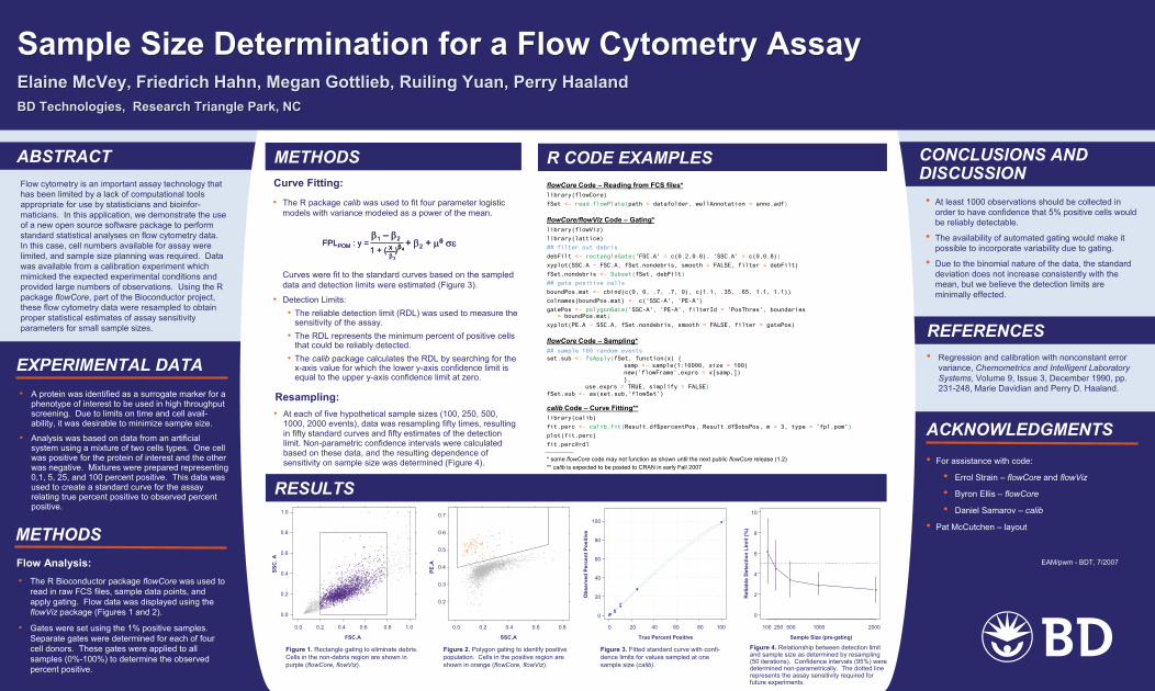
Figure 1. Rectangle gating to eliminate debris. Cells in the non-debris region are shown in purple (flowCore, flowViz).

Figure 2. Polygon gating to identify positive population. Cells in the positive region are shown in orange (flowCore, flowViz).

Figure 3. Fitted standard curve with confi-dence limits for values sampled at one sample size (calib).

Figure 4. Relationship between detection limit and sample size as determined by resampling (50 iterations). Confidence intervals (95%) were determined non-parametrically. The dotted line represents the assay sensitivity required for future experiments.

1.0

0.8

0.6

0.4

0.2

0.0

0.7

0.6

0.5

0.4

0.3

0.2

100

80

60

40

20

0

10

8

6

4

2

0

0.0 0.2 0.4 0.6 0.8 0 20 40 60 80 1000.0 0.2 0.4 0.6 0.8 1.0 100 250 500 1000 2000

SSC

.A

PE.A

Obs

erve

d Pe

rcen

t Pos

itive

Rel

iabl

e D

etec

tion

Lim

it (%

)

True Percent Positive Sample Size (pre-gating)FSC.A SSC.A

β1 – β2

1 + ( x )β4

β3

FPLPOM : y = + β2 + μθ σεβ1 – β2

1 + ( x )β4

β3

FPLPOM : y = + β2 + μθ σε

CONCLUSIONS ANDDISCUSSION

REFERENCES

ABSTRACT

Sample Size Determination for a Flow Cytometry Assay- Elaine McVey, Friedrich Hahn, Megan Gottlieb, Ruiling Yuan, Perry Haaland

BD Technologies, Research Triangle Park, NC

Sample Size Determination for a Flow Cytometry Assay- Elaine McVey, Friedrich Hahn, Megan Gottlieb, Ruiling Yuan, Perry Haaland

BD Technologies, Research Triangle Park, NC

Flow cytometry is an important assay technology that has been limited by a lack of computational tools appropriate for use by statisticians and bioinfor-maticians. In this application, we demonstrate the use of a new open source software package to perform standard statistical analyses on flow cytometry data. In this case, cell numbers available for assay were limited, and sample size planning was required. Data was available from a calibration experiment which mimicked the expected experimental conditions and provided large numbers of observations. Using the R package flowCore, part of the Bioconductor project, these flow cytometry data were resampled to obtain proper statistical estimates of assay sensitivity parameters for small sample sizes.

• At least 1000 observations should be collected in order to have confidence that 5% positive cells would be reliably detectable.

• The availability of automated gating would make it possible to incorporate variability due to gating.

• Due to the binomial nature of the data, the standard deviation does not increase consistently with the mean, but we believe the detection limits are minimally effected.

METHODS

EXPERIMENTAL DATA

ACKNOWLEDGMENTS

JBA/pwm - BDT, 1/2007

• Errol Strain – flowCore/flowViz

• Byron Ellis – flowCore

• Daniel Samarov – calib

• Pat McCutchen – layout

• A protein was identified as a surrogate marker for a phenotype of interest to be used in high throughput screening. Due to limits on time and cell avail-ability, it was desirable to minimize sample size.

• Analysis was based on data from an artificial system using a mixture of two cells types. One cell was positive for the protein of interest and the other was negative. Mixtures were prepared representing 0,1, 5, 25, and 100 percent positive. This data was used to create a standard curve for the assay relating true percent positive to observed percent positive.

Sample Size Determination for a Flow Cytometry Assay- Elaine McVey, Friedrich Hahn, Megan Gottlieb, Ruiling Yuan, Perry Haaland

BD Technologies, Research Triangle Park, NC

Sample Size Determination for a Flow Cytometry Assay- Elaine McVey, Friedrich Hahn, Megan Gottlieb, Ruiling Yuan, Perry Haaland

BD Technologies, Research Triangle Park, NC

R CODE EXAMPLES

METHODS

• The R Bioconductor package flowCore was used to read in raw FCS files, sample data points, and apply gating. Flow data was displayed using the flowViz package (Figures 1 and 2).

• Gates were set using the 1% positive samples. Separate gates were determined for each of four cell donors. These gates were applied to all samples (0%-100%) to determine the observed percent positive.

• Regression and calibration with nonconstant error variance, Chemometrics and Intelligent Laboratory Systems, Volume 9, Issue 3, December 1990, pp. 231-248, Marie Davidian and Perry D. Haaland.

Flow Analysis:

Curve Fitting:

• The R package calib was used to fit four parameter logistic models with variance modeled as a power of the mean.

Curves were fit to the standard curves based on the sampled data and detection limits were estimated (Figure 3).

• Detection Limits:• The reliable detection limit (RDL) was used to measure the

sensitivity of the assay.• The RDL represents the minimum percent of positive cells

that could be reliably detected.• The calib package calculates the RDL by searching for the

x-axis value for which the lower y-axis confidence limit is equal to the upper y-axis confidence limit at zero.

Resampling:• At each of five hypothetical sample sizes (100, 250, 500,

1000, 2000 events), data was resampling fifty times, resulting in fifty standard curves and fifty estimates of the detection limit. Non-parametric confidence intervals were calculated based on these data, and the resulting dependence of sensitivity on sample size was determined (Figure 4).

RESULTS

flowCore Code – Reading from FCS files*library(flowCore)

fSet <- read.flowPlate(path = datafolder, wellAnnotation=anno.adf)

flowCore/flowViz Code – Gating*library(flowViz)

library(lattice)

## filter out debris

debFilt <- rectangleGate('FSC.A' = c(0.2,0.8), 'SSC.A' = c(0,0.8))

xyplot(SSC.A ~ FSC.A, fSet.nondebris, smooth = FALSE, filter = debFilt)

fSet.nondebris <- Subset(fSet, debFilt)

## gate positive cells

boundPos.mat <- cbind(c(0, 0, .7, .7, 0), c(1.1, .35, .65, 1.1, 1.1))

colnames(boundPos.mat) <- c('SSC-A', 'PE-A')

gatePos <- polygonGate('SSC-A', 'PE-A', filterId = 'PosThres', boundaries = boundPos.mat)

xyplot(PE.A ~ SSC.A, fSet.nondebris, smooth = FALSE, filter = gatePos)

flowCore Code – Sampling*## sample 100 random eventsset.sub <- fsApply(fSet, function(x) {

samp <- sample(1:10000, size = 100)new('flowFrame',exprs = x[samp,])},

use.exprs = TRUE, simplify = FALSE)fSet.sub <- as(set.sub,'flowSet')

calib Code – Curve Fitting**library(calib)

fit.perc <- calib.fit(Result.df$percentPos, Result.df$obsPos, m = 3, type = 'fpl.pom')

plot(fit.perc)

fit.perc@rdl

* some flowCore code may not function as shown until the next public flowCore release (1.2)** calib is expected to be posted to CRAN in early Fall 2007

β1 – β2

1 + ( x )β4

β3

FPLPOM : y = + β2 + μθ σεβ1 – β2

1 + ( x )β4

β3

FPLPOM : y = + β2 + μθ σε

Figure 1. Rectangle gating to eliminate debris. Cells in the non-debris region are shown in purple (flowCore, flowViz).

Figure 2. Polygon gating to identify positive population. Cells in the positive region are shown in orange (flowCore, flowViz).

Figure 3. Fitted standard curve with confi-dence limits for values sampled at one sample size (calib).

Figure 4. Relationship between detection limit and sample size as determined by resampling (50 iterations). Confidence intervals (95%) were determined non-parametrically. The dotted line represents the assay sensitivity required for future experiments.

1.0

0.8

0.6

0.4

0.2

0.0

0.7

0.6

0.5

0.4

0.3

0.2

100

80

60

40

20

0

10

8

6

4

2

0

0.0 0.2 0.4 0.6 0.8 0 20 40 60 80 1000.0 0.2 0.4 0.6 0.8 1.0 100 500 1000 2000

SSC

A

PEA

Obs

erve

d Pe

rcen

t Pos

itive

Rel

iabl

e D

etec

tion

Lim

it (%

)

True Percent Positive Sample Size (pre-gating)FSC A SSC.A