sample sizes for self-controlled case series studiesstatistics.open.ac.uk/sccs/sccs_ssize.pdf ·...

Sample sizes for self-controlled case series studies

Patrick Musonda1, C. Paddy Farrington1 and Heather J. Whitaker1

1 Department of Statistics, The Open University, Milton Keynes, MK7 6AA, UK.

SUMMARY

We derive several formulae for the sample size required for a study designed using the self-controlled

case series method without age effects. We investigate these formulae by simulation, and identify one

based on the signed root likelihood ratio statistic which performs well. We extend this method to allow

for age effects, which can have a big impact on the sample size needed. This more general sample size

formula is also found to perform well in a broad range of situations.

KEY WORDS: epidemiology; likelihood ratio; power; sample size; self-controlled case series

Copyright c© 200 John Wiley & Sons, Ltd.

This is a preprint of an article accepted for publication in Statistics in Medicine Copyright c©2005 John Wiley

and sons, Ltd.

∗Correspondence to: C.P. Farrington. Department of Statistics, The Open University, Milton Keynes, MK7

6AA, UK. E-mail:[email protected]

Contract/grant sponsor: HJW and CPF were supported by a grant from the Wellcome Trust; contract/grant

number: 070346

Contract/grant sponsor: PM was supported by an EPSRC CASE studentship with funding from

GlaxoSmithKline Biologicals; contract/grant number: 0307

SAMPLE SIZES FOR SELF-CONTROLLED CASE SERIES STUDIES 1

1. INTRODUCTION

The self-controlled case series method (or case series method for short) is a modified cohort

method for estimating the relative incidence of specified events in a defined period after a

transient exposure. The method is based on a retrospective cohort model applied to a defined

observation period, conditionally on the number of events experienced by each individual over

the observation period. Time within the exposure period is classified as at risk or as control

time, in relation to exposures that are regarded as fixed. The key advantage of the method is

that it permits valid inference about the relative incidence of events in risk periods relative to

the control period, using only data on cases. A further benefit of the method is that it controls

for all fixed confounders, measured or otherwise, and allows for age-variation in the baseline

incidence of events. The method was originally published by Farrington [1] as a method for

evaluating vaccine safety, but has been used in various areas of epidemiology, in particular in

pharmaco-epidemiology. Whitaker et al [2] provide a detailed tutorial giving an account of the

theory and its applications, a discussion of modelling issues and implementation details in a

range of software packages. The case series method also applies to continuous exposures [3],

but here we will consider only binary exposures.

Our aim is to develop and evaluate a sample size formula for the method. A sample size

formula based on asymptotic calculations, applicable when there are no age effects, had been

proposed in an earlier publication, and our starting point was to evaluate this formula [4].

We soon discovered that it was inaccurate, and so began a search for a better expression.

Furthermore, age effects have a big effect on the power of case series models (and indeed

all types of models). Age effects are of critical importance in many settings, for example

applications to paediatric vaccines. Thus we sought a sample size formula that could be

generalised to allow for age effects, and that would work in the presence of such effects.

In Section 2 we present a brief motivating example. Then in Section 3, the notation and

the case series likelihood are introduced. A full description of the method is not included here:

this can be found in Whitaker et al. [2]. In Section 4 we propose four sample size formulae,

based on different asymptotic arguments. These formulae are derived under the assumption

Copyright c© 200 John Wiley & Sons, Ltd. Statist. Med. 200; 0:0–0

Prepared using simauth.cls

2 P. MUSONDA., C.P. FARRINGTON AND H.J. WHITAKER

that there are no age effects, and are evaluated in Section 5. In Section 6 we extend one of the

two best-performing methods to allow for age effects, and evaluate this more general formula

in Section 7. We conclude with a brief discussion in Section 8.

2. A MOTIVATING EXAMPLE

Idiopathic thrombocytopenic purpura (ITP) is an uncommon, potentially recurrent bleeding

disorder. Some studies have suggested that it can be caused by the measles, mumps and rubella

(MMR) vaccine, typically arising within 6 weeks of receipt of the vaccine. However, MMR-

induced ITP is uncommon, occurring about once every 22,000 MMR doses. Occurrence of ITP

does not constitute a contra-indication to MMR vaccination. Thus the possible association

between MMR vaccination and ITP can be studied using the case series method.

To design such a study, the first step is to select the period of observation. The recommended

age for primary MMR immunisation is 15 months. Thus we take the observation period to

include the second year of life (days 366 to 730 of life inclusive). Most primary MMR vaccines

are given in the period 12-18 months, though vaccination may be delayed in some cases. We

shall assume that 90% of the population receives MMR vaccine by age 2 years. The background

incidence of ITP during the second year of life is highest in the first quarter, and declines

thereafter.

To do a case series analysis, past cases of ITP with onset within the second year of life are

sampled, for example from hospital admission records. Their MMR vaccination status is then

ascertained up to age 730 days. The analysis is described in Whitaker et al. [2]. The issue of

interest in the present paper is how many cases should be selected to achieve a given power.

3. BACKGROUND AND NOTATION

In the following two sections we will be concerned only with situations where the underlying

(or baseline) incidence of an adverse event is constant, that is, does not vary with age (or time,

if time is the relevant time line). At each time point, an individual is categorised as exposed




or unexposed. Typically, the times at which an individual is exposed occur within a defined

time interval following an acute event, for example receipt of a drug. In other situations, the

exposure period might refer to the time spent on the drug. The period of exposure is called

the risk period.

We further assume that all individuals are followed up for an observation period of the same

length, and that a proportion p of individuals in the population spend some of this observation

period in an exposed state. For simplicity, we assume that each exposed individual spends a

proportion r of the observation period in the exposed state. (In practice, the observation and

risk periods vary between individuals, but this variation can reasonably be ignored for the

purposes of sample size calculations.) Thus if w is the length of the risk period and W is the

duration of the observation period, then r = w/W . Usually, w and W will be specified in the

design. However, only their ratio r is required.

During the risk period, the baseline incidence of an adverse event is increased by a

multiplicative factor ρ = eβ , where ρ is the relative incidence. The parameter ρ (or β) is the

focus of inference. Under the null hypothesis , ρ = 1, whereas under the alternative hypothesis

we specify some value for ρ 6= 1, the value we wish the study to detect.

A case is an individual who experiences at least one event during the observation period.

Suppose that a sample of cases is available, and that a total of n events arise in these cases.

Note that n refers to events, not individuals: the case series method allows multiple events per

individual, provided that these events are independent. Our sample size formulae will generally

relate to numbers of events, though in Section 6 we briefly touch upon estimating the number of

cases required. (If the event of interest is non-recurrent, then the case series method still applies

provided the event is rare.) Of these n events, suppose that n1 arise in exposed individuals,

that is, individuals who were exposed at some time during the observation period. Suppose

also that n0 events arise in unexposed individuals, that is, individuals who were not exposed

during the observation period. Of the n1 events in exposed individuals, suppose that x arise

in a risk period. Then the case series log likelihood is:




l(ρ) = x log(

ρr

ρr + 1− r

)+ (n1 − x) log

(1− r

ρr + 1− r

). (1)

Note that this is a binomial likelihood with binomial proportion π = ρr/(ρr + 1 − r), and

that it does not involve n0: only exposed individuals contribute to the log likelihood when

there are no age effects. The likelihood ratio statistic for the test of H0 : ρ = 1 is thus

D = 2 {l(ρ̂)− l(1)} = 2 {x log(ρ̂)− n1 log (ρ̂r + 1− r)} . (2)

Finally, note that, in large samples, we have

n ' n11 + pr(ρ− 1)p(ρr + 1− r)

. (3)

In particular, if ρ = 1 then n ' n1/p.

4. SAMPLE SIZE FORMULAE WITHOUT AGE EFFECTS

In this section we describe four candidate sample size formulae based on different asymptotic

approximations, assuming there is no age effect. The significance level is denoted α, the power

is γ, z1−α/2 is the (1− α2 )-quantile of the standard normal distribution, and zγ is its γ-quantile.

For simplicity, the formulae quoted are for n1, the total number of events required in exposed

individuals. For the last method described, formulae for both n1 and n are given, as this

formula will later be generalized.

4.1 Sample size formula based on the sampling distribution of ρ

This method was described by Farrington et al. [4]. The idea is to use ρ̂ as the test statistic,

and base the sample size formula on its asymptotic normal distribution. The asymptotic

variance of ρ̂ may be obtained by twice differentiating (−1) times expression (1) with respect

to ρ, taking expectations, and inverting the result. This yields the expression

var(ρ̂) ' 1n1

ρ(ρr + 1− r)2

r(1− r).




Thus under the null hypothesis, ρ̂ ≈ N(1, 1

n1r(1−r)

)and under the alternative, ρ̂ ≈

N(ρ, ρ(ρr+1−r)2

n1r(1−r)

). This leads to the following expression for the sample size:

n1 =1

r(1− r)(ρ− 1)2×[z1−α/2 + zγ(ρr + 1− r)

√ρ]2

. (4)

4.2 Sample size formula based on the sampling distribution of β

A concern about (4) is that the sampling distribution of ρ̂ may not be symmetric in

small samples. Thus we derived a sample size formula based on the sampling distribution

of β = log(ρ), in the hope that this might be less skewed. We have

var(β̂) ' 1n1

(ρr + 1− r)2

ρr(1− r).

Under the null hypothesis, β̂ ≈ N(0, 1

n1r(1−r)

)whereas under the alternative, β̂ ≈

N(β, (ρr+1−r)2

n1ρr(1−r)

). This leads to the following expression for the sample size:

n1 =1

r(1− r) log(ρ)2×[z1−α/2 + zγ(ρr + 1− r)/

√ρ]2

. (5)

4.3 Sample size formula based on the binomial proportion

As described in Section 3, in the simplified setting we are considering, the log likelihood

is that of a binomial with proportion π = ρr/(ρr + 1 − r). There is a substantial

literature on sample size formulae for binomial proportions. A popular expression is based

on the arcsine variance-stabilizing transformation [5]. The test statistic is T = arcsin(√

π̂);

under the null hypothesis T ≈ N(arcsin(

√r), 1

4n1

), while under the alternative, T ≈

N(arcsin(

√ρr/(ρr + 1− r)), 1

4n1

). Thus we obtain the following expression for the sample

size:

n1 =(z1−α/2 + zγ)2

4[arcsin

(√ρr/(ρr + 1− r)

)− arcsin(

√r)]2 . (6)

4.4 Sample size formula based on the signed root likelihood ratio




A limitation of the sample size based on the binomial log-likelihood is that it is not readily

extended to handle age effects since the likelihood is then multinomial. Furthermore, the

most convenient test to use to decide whether the exposure is associated with the outcome is

the likelihood ratio test. Thus it makes sense to base the sample size on the likelihood ratio

statistic (2). Under the null hypothesis, the likelihood ratio statistic has the χ2(1) distribution,

asymptotically. To obtain an asymptotically normal test statistic, we use the signed root

likelihood ratio:

T = sgn(β̂)√

2{

xβ̂ − n1 log(eβ̂r + 1− r

)}where

β̂ = log(

x(1− r)r(n1 − x)

).

Under the null hypothesis, T ≈ N(0, 1), and under the alternative hypothesis, T ≈

N(sgn(β)√

n1A1, B1) where

A1 = 2[(

eβr

eβr + 1− r

)β − log(eβr + 1− r)

],

B1 =β2

A1

eβr(1− r)

(eβr + 1− r)2.

These expressions are derived in the Appendix. They lead to the following expression for

n1:

n1 =

(z1−α/2 + zγ

√B1

)2A1

. (7)

More generally suppose that a proportion p of the population are exposed. Then T ≈

N(sgn(β)√

nA, B), where

A = 2p(ρr + 1− r)1 + pr(ρ− 1)

[(eβr

eβr + 1− r

)β − log(eβr + 1− r)

], (8)

B =β2

A

p(ρr + 1− r)1 + pr(ρ− 1)

eβr(1− r)

(eβr + 1− r)2.




The sample size n required is then

n =

(z1−α/2 + zγ

√B)2

A. (9)

Note that n and n1 from expressions (9) and (7) are in the ratio determined by (3).

5. COMPARATIVE EVALUATION

In Section 4 four expressions for the sample size were obtained, based on different asymptotic

arguments. In this section we describe the evaluation of these four expressions.

5.1. Simulation study

We carried out a simulation study as follows. We fixed an observation period of 500 time units

(for example, days) and assumed that the entire population was exposed in this time interval,

so that p = 1. The ratio of the risk period to the observation period, r, took values 0.01, 0.05,

0.1 and 0.5 (corresponding to 5, 25, 50 and 250 time units, respectively). We evaluated values

of the relative incidence ρ equal to 0.5, 1.5, 2, 3, 5 and 10. The significance level was set at

5%, and the power at 80% or 90%. The combination of four values of r, six values of ρ, two

powers, and four sample size formulae thus required 192 different simulations. Each simulation

involved 2000 runs.

The sample sizes were calculated using expressions (4 - 7). We rounded the sample size

up to the next integer. For each run we randomly allocated each event to the risk or the

control period, fitted the case series model, and carried out the likelihood ratio test of the null

hypothesis ρ = 1. The empirical power is the percentage of the 2000 runs in which the null

hypothesis was rejected by the likelihood ratio test at the 5% significance level. The Monte

Carlo standard error for the empirical power is about 0.89% at 80% power and 0.67% at 90%

power.




5.2. Results

The results for 80% power are shown in Table 1, and those for 90% power are shown in Table

2. It is clear that expressions (4) and (5) are inaccurate. For relative incidences greater than

1, expression (4) tends to under-estimate and expression (5) tends to overestimate the sample

size required when ρ > 1. This is most likely due to skewness of the sampling distributions of

ρ and β. In contrast, expressions (6) and (7) are much more accurate, giving powers close to

the nominal values across the parameter ranges.

5.3. A note on sample sizes

To avoid clutter we have not presented the sample sizes in Tables 1 and 2. A noteworthy

feature is the non-monotonic relation between sample size and power. For example, consider

the results in Table 1 for r = 0.01 and ρ = 5. The empirical powers for the four sample size

formulae (4 - 7) are, respectively, 80%, 95%, 77% and 84%. The sample sizes these simulations

are based on are 97, 216, 135 and 119, respectively. Thus a sample size of 135 gives 77% power,

yet 119 gives 84% power. The non-monotonicity of the power curve is due to the discreteness of

the data, and has been discussed by Chernick and Liu [6] One consequence of this phenomenon

is that there may be no unique ‘correct’ sample size, though it may be possible to specify a

range of values over which a study will have adequate power, or the minimum such value. We

shall not dwell on this issue any further, but instead turn to the practically important problem

of allowing for age effects in sample size determination.

6. SAMPLE SIZE FORMULA WITH AGE EFFECT

The sample size formulae derived in Section 4 apply to a simplified situation in which there

are no age effects. In practice, strong age effects may be present. Such age effects can have a

big effect on study power, and must be taken into account in sample size calculations.

In Section 5, sample size formulae (6) and (7) were found to be most accurate. Expression

(6) is based on binomial proportions, and thus cannot readily be extended to allow for age

effects, since the likelihood becomes multinomial when age effects are allowed for. However,




sample size formula (7) based on the likelihood ratio test can be extended to allow for age

effects.

In line with the parametric case series models described in Whitaker et al. [2], in which age

effects are modelled using a step function, we shall assume that the age-specific incidence is

piecewise constant. In practical applications, we have found this approach for specifying the

age effect both convenient and flexible.

6.1. Assumptions and notation

We again consider a simplified scenario, but involving age effects. We assume that all

individuals are followed over the same observation period, which covers J age groups of

duration ej , j = 1, 2, ..., J. Suppose that the probability that an individual is exposed in

age group j is pj . The probability that an individual, randomly selected from the population,

is unexposed during the observation period is p0 = 1−∑J

j=1 pj .

We suppose furthermore that if an individual is exposed in age group j, the post-exposure

risk period, of length e∗, is entirely contained within age group j. This assumption greatly

simplifies the calculations, by avoiding any overlaps. It implies that e∗ ≤ ej for all age groups

j = 1, ..., J . This should not be too restrictive in practice, at least when the risk period is

short.

Finally, let δj denote the logarithm of the age-specific relative incidence, relative to age

group 1, so that δ1 = 0. We assume that these age effects are known. As before, ρ denotes the

relative incidence associated with the exposure, and β its logarithm.

6.2. Sample size formula allowing for age effects

The full derivation is given in the Appendix. The sample size formula involves the following

intermediate quantities. First, let rj denote the weighted ratio of time at risk to the overall

risk period:

rj =eδj e∗∑J

s=1 eδses

, j = 1, ..., J .




Note that if there are no age effects (δj = 0 for all j) then rj = r, the ratio of the risk period

to the observation period defined in Section 3. Second, let πj denote the probability, for an

individual exposed in age group j, that an event arising in age group j occurs during the

exposure period:

πj =rjρ

rjρ + 1− rj, j = 1, ..., J .

If there are no age effects, then πj = π, the binomial probability defined in Section 3. Finally,

let νj denote the probability that a case is exposed in age group j:

νj =pj (rjρ + 1− rj)

p0 +∑J

s=1 ps (rsρ + 1− rs), j = 1, ..., J . (10)

Note that if there is no association between exposure and outcome, so that ρ = 1, then νj = pj ,

the population proportion exposed. If there is an association, however, the age distribution of

exposure in the cases will usually differ from that of the general population. If there is no age

effect, then νj = n1/n from expression (3). Now define the following constants A and B.

A = 2J∑

s=1

νs

[πsβ − log(rse

β + 1− rs)], (11)

B =β2

A

J∑s=1

νsπs(1− πs).

Note that when there are no age effects then A and B reduce to the expressions (8). The total

number of events required for 100γ% power at the 100α% significance level is:

n =

(z1−α/2 + zγ

√B)2

A. (12)

If there are no age effects, this reduces to expression (9).

6.3. Sample size formulae for the number of cases

So far we have presented formulae for n, the number of events. To obtain a sample size formula

for the number of cases, an estimate of the cumulative incidence over the observation period is




required. Let Λ denote this cumulative incidence. Then under the Poisson model, the number

of cases required (that is, the number of individuals with one or more events), nc, is

nc = n

(1− e−Λ

Λ

).

Generally, Λ is not known with any accuracy. In practice, most applications of the case series

method are to situations where Λ is very small, in which case nc ' n. Furthermore, the

independence of repeat events may be open to doubt. For these reasons, we would generally

advise taking nc = n.

7. EVALUATION WITH AGE EFFECTS

7.1. Simulation study

We evaluated the sample size expression (12) as follows. As before, we assumed an observation

period stretching for 500 time units, but now partitioned into J = 5 age intervals of 100

days. We fixed the age-specific proportions pj of the population exposed, and assumed that

all individuals in the population are exposed, but varied the age effect: increasing, symmetric

and decreasing. The parameter values we used are shown in Table 3.

The risk period durations e∗ must be less than the shortest age group, and were set at 5,

10 and 50 days. For comparability with Tables 1 and 2, these are reported as proportions of

the overall observation period and are denoted r. Thus r = 0.01, 0.05 and 0.1. The values for

ρ were the same as in the previous simulations. We evaluated the sample size for powers of

80% and 90%, at 5% significance level. The combination of three values of r, six values of ρ,

two powers, and three age effects required 108 different simulations; each involved 5000 runs.

The sample sizes were calculated using expression (12) and were rounded up to the next

integer. For each simulation, we randomly and independently allocated the exposure to an

age group and the event to an age and exposure group combination. Since the simulations are

conditional on an event occurring, we use the age-specific exposure probabilities defined by

expression (10) to perform this allocation. We then fitted the case series model with five age

groups (and thus four age parameters), and carried out the likelihood ratio test of the null




hypothesis ρ = 1. The Monte Carlo standard error for the empirical power is about 0.57% at

80% power and 0.42% at 90% power.

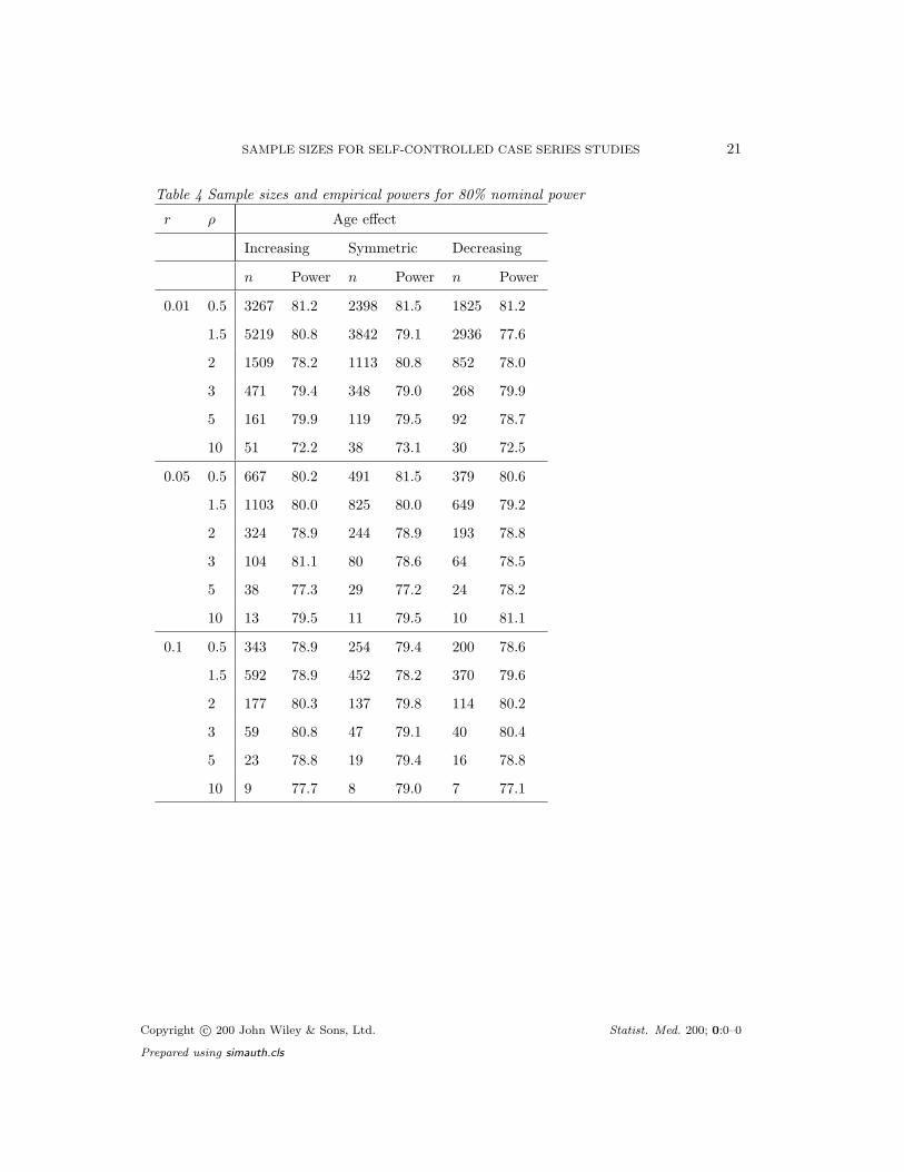
7.2. Results

The sample sizes and empirical powers are shown in Table 4 (for 80% power) and Table 5

(for 90% power). Note that, since p0 = 0, n = n1. The empirical powers generally correspond

closely to the nominal values, across the range of parameter values and age settings. There

is one exception, namely the rather low (72-73%) power obtained for the 5-day risk period

(r = 0.01) when ρ = 10. This occurred only for nominal power of 80%.

7.3. Example

We now return to the example of Section 2. The observation period includes the ages 366 to

730 days, which we subdivide into J = 4 periods of lengths e1 = e2 = e3 = 91 days, and

e4 = 92 days. We take the proportions vaccinated in each of these age intervals to be p1 = 0.6,

p2 = 0.2, p3 = 0.05, p4 = 0.05. We take the age effects to be eδ1 = 1, eδ2 = 0.6, eδ3 = eδ4 = 0.4.

The risk period is e∗ = 42 days. We set ρ = 3, z1−α/2 = 1.96 and zγ = 0.8416 for 80% power

to detect a relative incidence of 3 at the 5% significance level.

With these values we find n = 37. Had we ignored the age effect we would have obtained

n = 45.

8. DISCUSSION

This paper presents three main findings. First, we have established that the sample size formula

published by Farrington et al. [4] is not accurate, as demonstrated in Tables 1 and 2. Second,

we have found that a sample size formula based on the signed root likelihood ratio performs

well under a wide range of scenarios, as shown in Tables 1, 2, 4 and 5. Third, the type of age

effects has a big impact on the sample size required, as shown in Tables 4 and 5. Thus it is

important to allow for such age effects in calculating the sample size. We also investigated

other approaches, not reported here, in particular one based on a second-order approximation




to the variance of β̂, and another involving a continuity correction. These did not provide

any marked improvements in accuracy. In conclusion, we recommend the sample size formula

based on the signed root likelihood ratio, as shown in expressions (9) and (12).

Our empirical power calculations were based on the likelihood ratio test. In practice,

statistical significance is sometimes assessed by calculating the 95% confidence interval for

the relative incidence, and observing whether this confidence interval includes 1. We also

evaluated our recommended sample size formula using this second criterion. The empirical

powers were generally close to the nominal values, except for large relative risks and/or very

short risk periods when such confidence intervals can be markedly non-central.

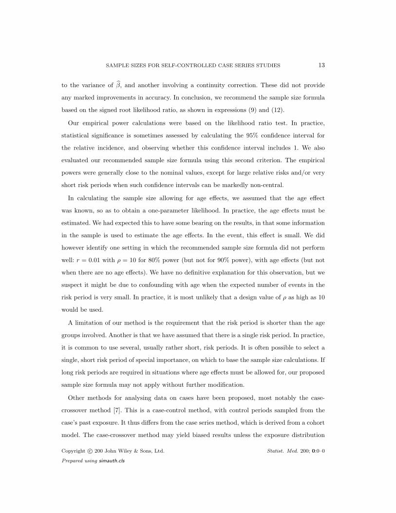
In calculating the sample size allowing for age effects, we assumed that the age effect

was known, so as to obtain a one-parameter likelihood. In practice, the age effects must be

estimated. We had expected this to have some bearing on the results, in that some information

in the sample is used to estimate the age effects. In the event, this effect is small. We did

however identify one setting in which the recommended sample size formula did not perform

well: r = 0.01 with ρ = 10 for 80% power (but not for 90% power), with age effects (but not

when there are no age effects). We have no definitive explanation for this observation, but we

suspect it might be due to confounding with age when the expected number of events in the

risk period is very small. In practice, it is most unlikely that a design value of ρ as high as 10

would be used.

A limitation of our method is the requirement that the risk period is shorter than the age

groups involved. Another is that we have assumed that there is a single risk period. In practice,

it is common to use several, usually rather short, risk periods. It is often possible to select a

single, short risk period of special importance, on which to base the sample size calculations. If

long risk periods are required in situations where age effects must be allowed for, our proposed

sample size formula may not apply without further modification.

Other methods for analysing data on cases have been proposed, most notably the case-

crossover method [7]. This is a case-control method, with control periods sampled from the

case’s past exposure. It thus differs from the case series method, which is derived from a cohort

model. The case-crossover method may yield biased results unless the exposure distribution




is exchangeable across case and control periods [8]. In particular, it requires the age-specific

exposure probability to be constant. In contrast, the case series method allows for age effects.

The sample size formulae presented in this paper help to emphasize the importance of taking

such effects into account at the design stage.




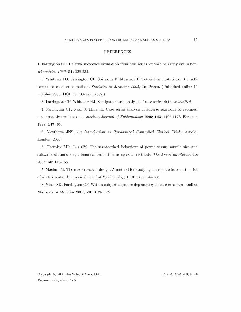
REFERENCES

1. Farrington CP. Relative incidence estimation from case series for vaccine safety evaluation.

Biometrics 1995; 51: 228-235.

2. Whitaker HJ, Farrington CP, Spiessens B, Musonda P. Tutorial in biostatistics: the self-

controlled case series method. Statistics in Medicine 2005; In Press. (Published online 11

October 2005, DOI: 10.1002/sim.2302.)

3. Farrington CP, Whitaker HJ. Semiparametric analysis of case series data. Submitted.

4. Farrington CP, Nash J, Miller E. Case series analysis of adverse reactions to vaccines:

a comparative evaluation. American Journal of Epidemiology 1996; 143: 1165-1173. Erratum

1998; 147: 93.

5. Matthews JNS. An Introduction to Randomized Controlled Clinical Trials. Arnold:

London, 2000.

6. Chernick MR, Liu CY. The saw-toothed behaviour of power versus sample size and

software solutions: single binomial proportion using exact methods. The American Statistician

2002; 56: 149-155.

7. Maclure M. The case-crossover design: A method for studying transient effects on the risk

of acute events. American Journal of Epidemiology 1991; 133: 144-153.

8. Vines SK, Farrington CP. Within-subject exposure dependency in case-crossover studies.

Statistics in Medicine 2001; 20: 3039-3049.




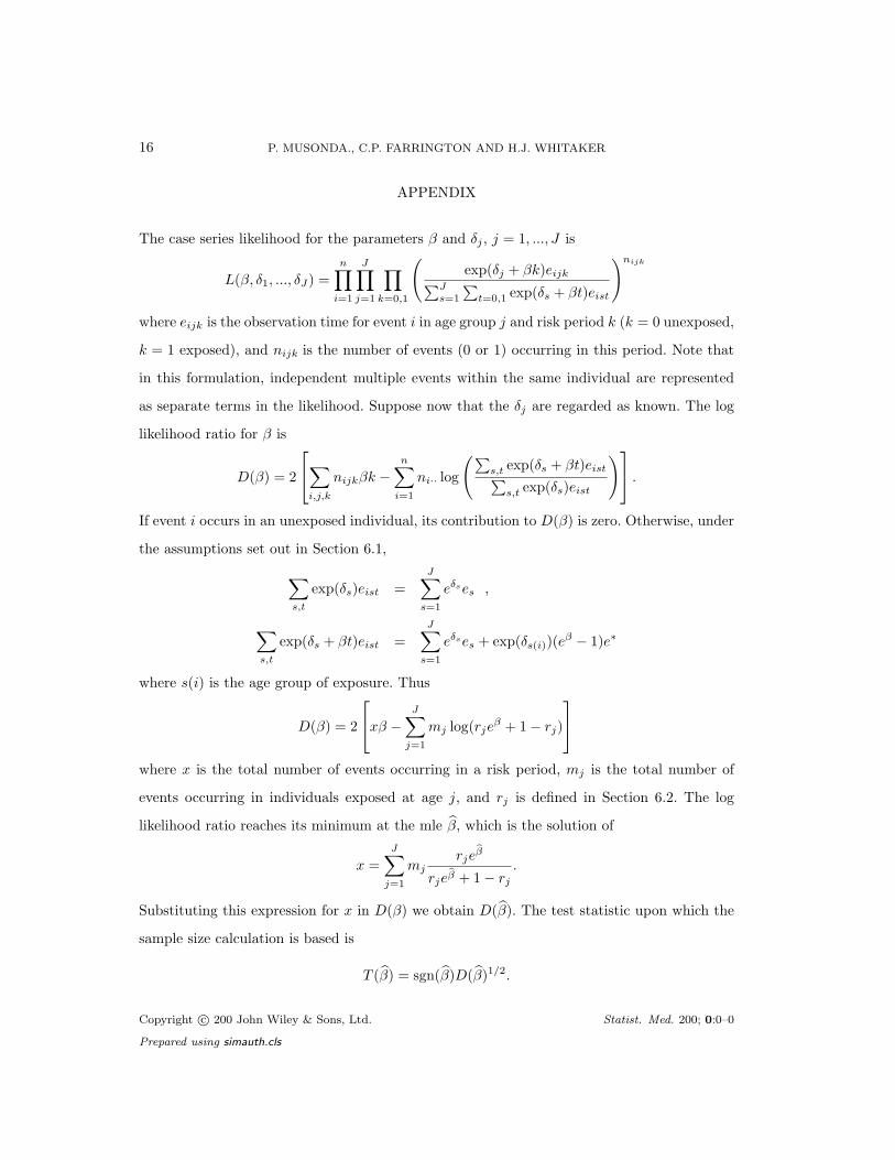
APPENDIX

The case series likelihood for the parameters β and δj , j = 1, ..., J is

L(β, δ1, ..., δJ) =n∏

i=1

J∏j=1

∏k=0,1

(exp(δj + βk)eijk∑J

s=1

∑t=0,1 exp(δs + βt)eist

)nijk

where eijk is the observation time for event i in age group j and risk period k (k = 0 unexposed,

k = 1 exposed), and nijk is the number of events (0 or 1) occurring in this period. Note that

in this formulation, independent multiple events within the same individual are represented

as separate terms in the likelihood. Suppose now that the δj are regarded as known. The log

likelihood ratio for β is

D(β) = 2

∑i,j,k

nijkβk −n∑

i=1

ni·· log

(∑s,t exp(δs + βt)eist∑

s,t exp(δs)eist

) .

If event i occurs in an unexposed individual, its contribution to D(β) is zero. Otherwise, under

the assumptions set out in Section 6.1,∑s,t

exp(δs)eist =J∑

s=1

eδses ,

∑s,t

exp(δs + βt)eist =J∑

s=1

eδses + exp(δs(i))(eβ − 1)e∗

where s(i) is the age group of exposure. Thus

D(β) = 2

xβ −J∑

j=1

mj log(rjeβ + 1− rj)

where x is the total number of events occurring in a risk period, mj is the total number of

events occurring in individuals exposed at age j, and rj is defined in Section 6.2. The log

likelihood ratio reaches its minimum at the mle β̂, which is the solution of

x =J∑

j=1

mjrje

β̂

rjeβ̂ + 1− rj

.

Substituting this expression for x in D(β) we obtain D(β̂). The test statistic upon which the

sample size calculation is based is

T (β̂) = sgn(β̂)D(β̂)1/2.




The asymptotic variance of β̂ is

V (β̂) =

J∑j=1

mjπj(1− πj)

−1

where the πj are defined in Section 6.2. Expanding T (β̂) in a Taylor series around β, and

substituting V (β̂) we obtain, to first order in n,

E[T (β̂)] ' sgn(β)

2J∑

j=1

mj

[βπj − log(rje

β + 1− rj)]

1/2

,

V [T (β̂)] ' β2{E[T (β̂)]

}2

J∑j=1

mjπj(1− πj).

Finally, replace mj by nνj , with νj defined as in Section 6.2. Thus T (β̂) ≈ N(sgn(β)√

nA, B)

where A and B are given in equations (11). Note that, by expanding A and B to second order

in β, it can be shown that A → 0 and B → 1 as β → 0, as expected.




Table 1 Empirical power for 80% nominal value

Sample Size Expression Sample Size Expression

r ρ (4) (5) (6) (7) r ρ (4) (5) (6) (7)

0.01 0.5 81 80 81 81 0.1 0.5 86 73 82 84

1.5 78 84 80 78 1.5 75 82 80 79

2 76 87 82 81 2 75 85 81 80

3 78 88 79 80 3 64 84 81 80

5 80 95 77 84 5 64 89 79 84

10 79 98 80 79 10 79 96 79 80

0.05 0.5 84 80 80 82 0.5 0.5 92 77 79 81

1.5 77 84 81 79 1.5 73 80 80 80

2 76 85 80 79 2 77 76 76 81

3 70 88 84 80 3 77 81 81 81

5 80 95 82 80 5 76 88 79 79

10 63 98 79 78 10 97 81 81 81




Table 2 Empirical power for 90% nominal value

Sample Size Expression Sample Size Expression

r ρ (4) (5) (6) (7) r ρ (4) (5) (6) (7)

0.01 0.5 91 87 89 89 0.1 0.5 92 90 90 89

1.5 88 92 91 90 1.5 89 91 90 90

2 90 91 90 89 2 89 90 89 90

3 86 93 89 90 3 85 91 91 89

5 87 96 91 91 5 93 95 89 91

10 85 99 90 89 10 97 97 91 89

0.05 0.5 92 90 91 89 0.5 0.5 95 91 91 91

1.5 89 92 90 91 1.5 90 89 90 90

2 90 84 90 89 2 87 90 90 90

3 84 94 91 91 3 95 90 91 92

5 86 93 91 90 5 96 95 89 89

10 86 99 89 93 10 100 97 92 92




Table 3 Exposure and age effects used in the simulations

Age group j

Parameter 1 2 3 4 5

Proportion exposed, pj 0.35 0.30 0.20 0.10 0.05

Age effect, eδj

Increasing 1 2 3 4 5

Symmetric 1 2 3 2 1

Decreasing 1 1/2 1/3 1/4 1/5




Table 4 Sample sizes and empirical powers for 80% nominal power

r ρ Age effect

Increasing Symmetric Decreasing

n Power n Power n Power

0.01 0.5 3267 81.2 2398 81.5 1825 81.2

1.5 5219 80.8 3842 79.1 2936 77.6

2 1509 78.2 1113 80.8 852 78.0

3 471 79.4 348 79.0 268 79.9

5 161 79.9 119 79.5 92 78.7

10 51 72.2 38 73.1 30 72.5

0.05 0.5 667 80.2 491 81.5 379 80.6

1.5 1103 80.0 825 80.0 649 79.2

2 324 78.9 244 78.9 193 78.8

3 104 81.1 80 78.6 64 78.5

5 38 77.3 29 77.2 24 78.2

10 13 79.5 11 79.5 10 81.1

0.1 0.5 343 78.9 254 79.4 200 78.6

1.5 592 78.9 452 78.2 370 79.6

2 177 80.3 137 79.8 114 80.2

3 59 80.8 47 79.1 40 80.4

5 23 78.8 19 79.4 16 78.8

10 9 77.7 8 79.0 7 77.1




Table 5 Sample sizes and empirical powers for 90% nominal power

r ρ Age effect

Increasing Symmetric Decreasing

n Power n Power n Power

0.01 0.5 4276 90.6 3139 89.0 2390 91.3

1.5 7073 89.7 5207 89.3 3978 89.5

2 2062 91.1 1520 88.8 1163 90.2

3 651 89.6 481 89.5 369 89.7

5 224 89.9 167 91.1 128 90.7

10 72 89.9 54 89.6 42 88.7

0.05 0.5 874 89.7 644 90.4 497 90.4

1.5 1493 90.3 1116 89.5 877 89.2

2 442 90.2 332 88.9 263 89.5

3 143 91.2 109 89.9 87 87.4

5 52 88.2 40 91.7 33 88.0

10 19 88.9 15 90.7 13 89.5

0.1 0.5 450 89.7 334 89.9 263 90.2

1.5 800 89.3 611 89.9 498 89.2

2 241 89.4 186 90.6 154 89.5

3 81 90.8 64 90.5 54 90.2

5 31 90.5 25 90.1 22 89.7

10 12 87.3 11 90.7 10 89.1



sample sizes for self-controlled case series studiesstatistics.open.ac.uk/sccs/sccs_ssize.pdf ·...

Documents