sampling and reconstruction - computer...
TRANSCRIPT
15-463: Computational PhotographyAlexei Efros, CMU, Fall 2011Many slides from
Steve Marschner
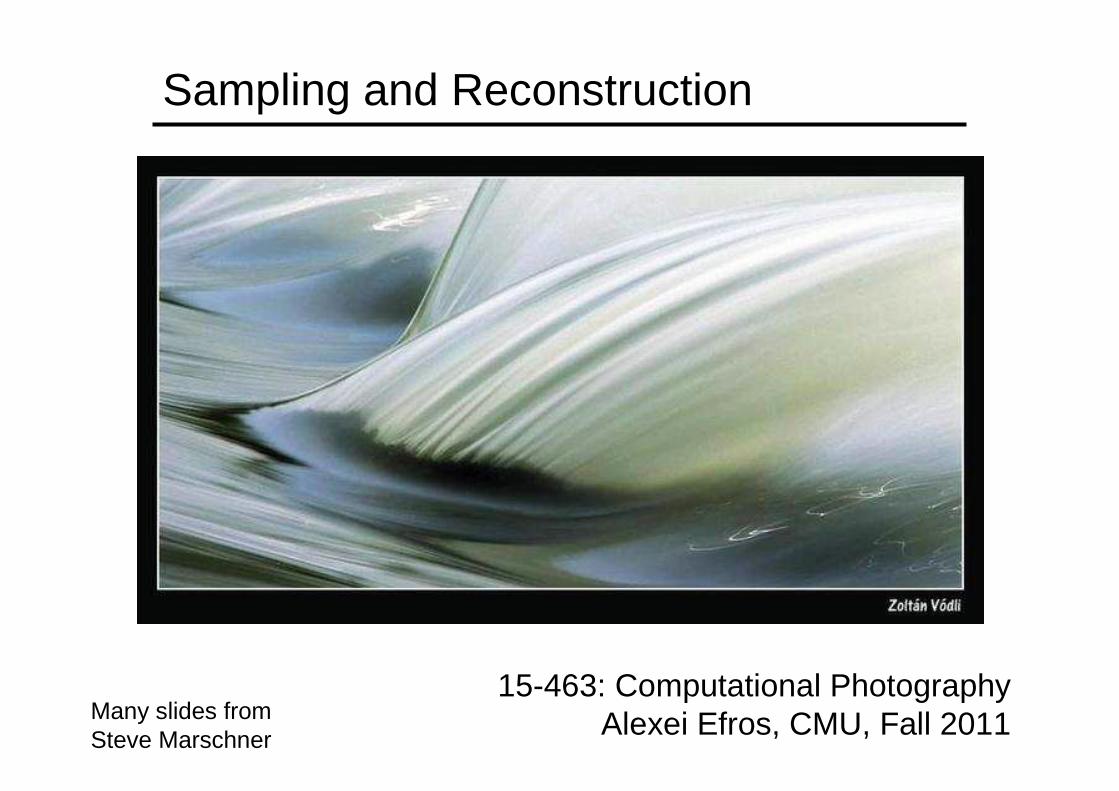
Sampling and Reconstruction
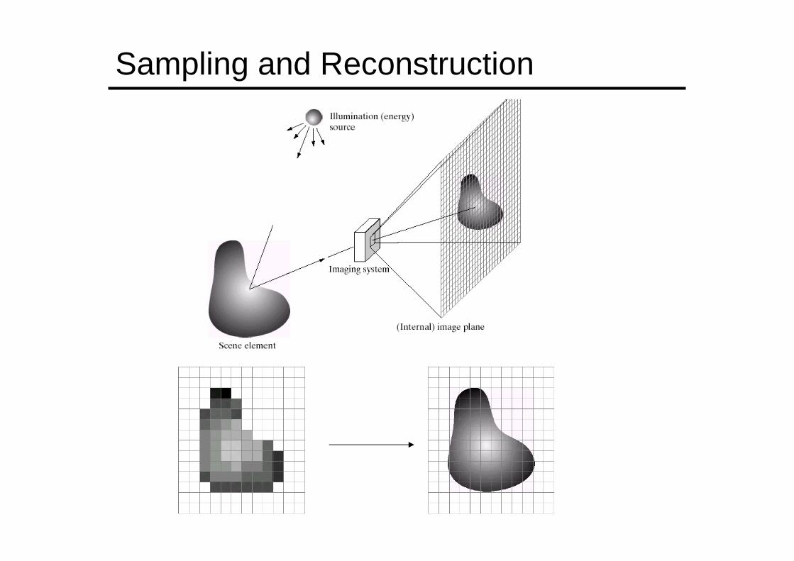
Sampling and Reconstruction
© 2006 Steve Marschner • 3
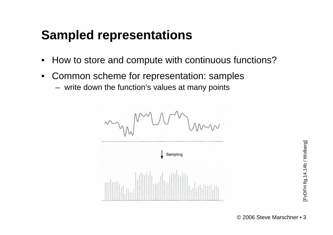
Sampled representations
• How to store and compute with continuous functions?
• Common scheme for representation: samples– write down the function’s values at many points
[FvD
FH
fig.1
4.14
b / W
olbe
rg]
© 2006 Steve Marschner • 4
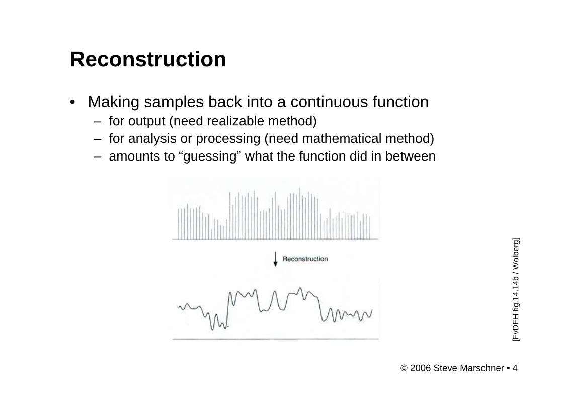
Reconstruction
• Making samples back into a continuous function– for output (need realizable method)– for analysis or processing (need mathematical method)– amounts to “guessing” what the function did in between
[FvD
FH
fig.1
4.14
b / W
olbe
rg]
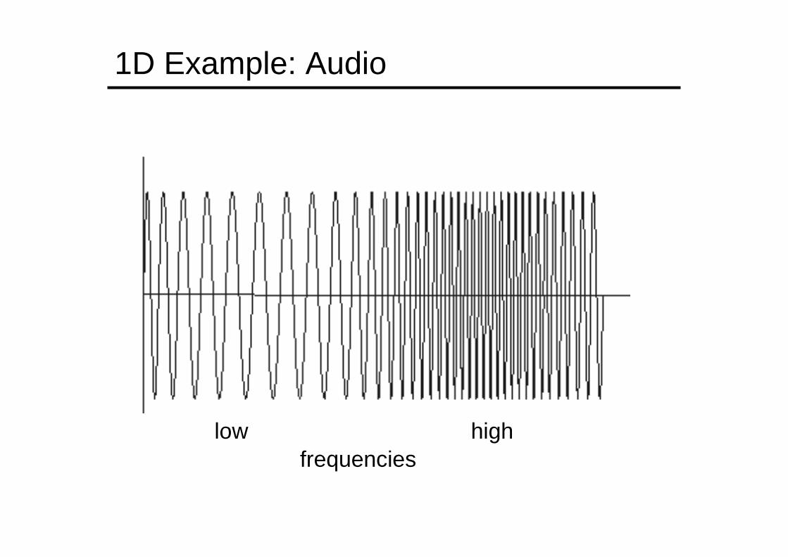
1D Example: Audio
low highfrequencies

© 2006 Steve Marschner • 6
Sampling in digital audio
• Recording: sound to analog to samples to disc
• Playback: disc to samples to analog to sound again– how can we be sure we are filling in the gaps correctly?
© 2006 Steve Marschner • 7
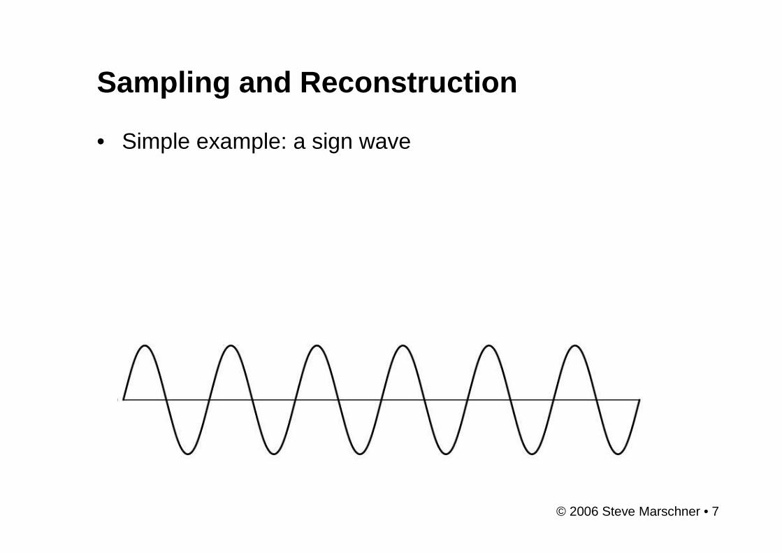
Sampling and Reconstruction
• Simple example: a sign wave
© 2006 Steve Marschner • 8
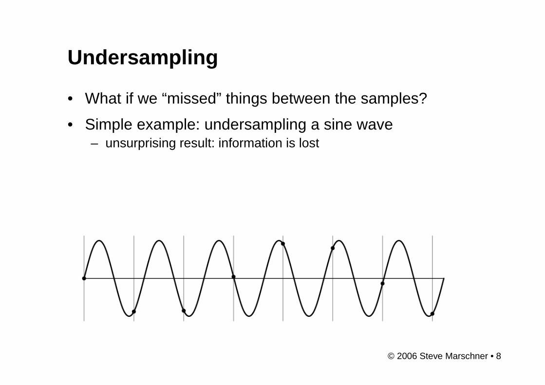
Undersampling
• What if we “missed” things between the samples?
• Simple example: undersampling a sine wave– unsurprising result: information is lost
© 2006 Steve Marschner • 9
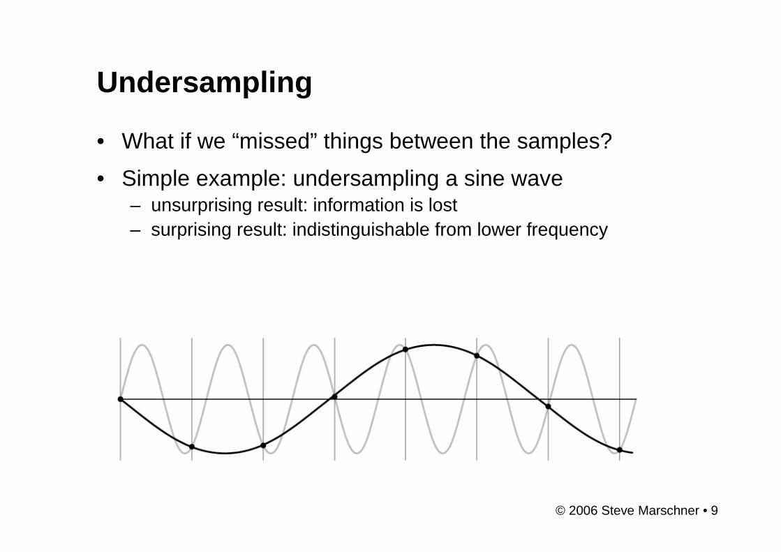
Undersampling
• What if we “missed” things between the samples?
• Simple example: undersampling a sine wave– unsurprising result: information is lost– surprising result: indistinguishable from lower frequency
© 2006 Steve Marschner • 10
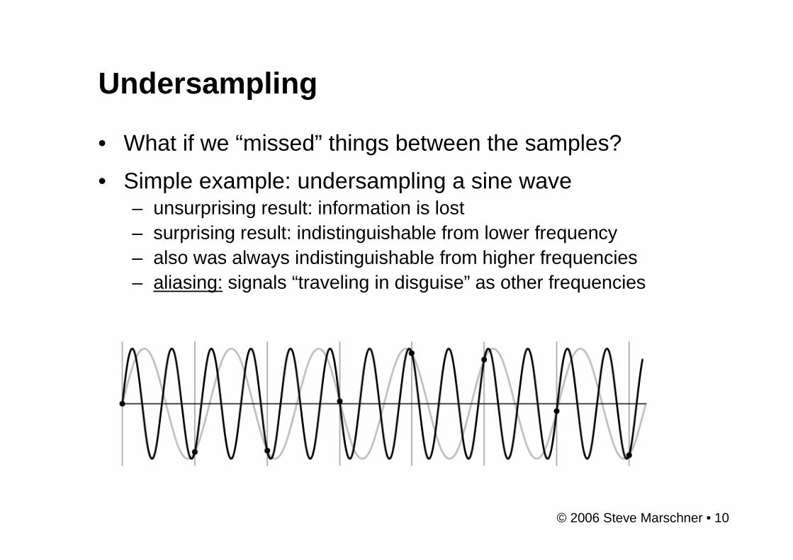
Undersampling
• What if we “missed” things between the samples?
• Simple example: undersampling a sine wave– unsurprising result: information is lost– surprising result: indistinguishable from lower frequency– also was always indistinguishable from higher frequencies– aliasing: signals “traveling in disguise” as other frequencies
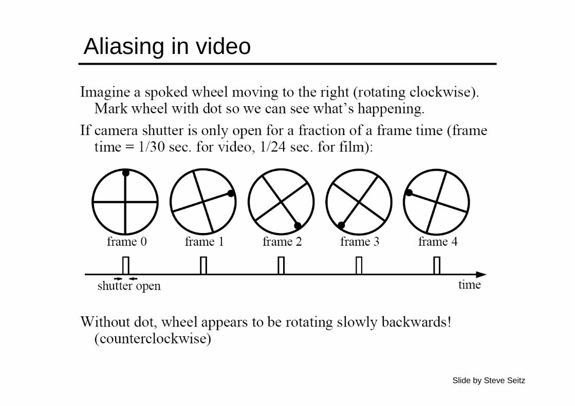
Aliasing in video
Slide by Steve Seitz
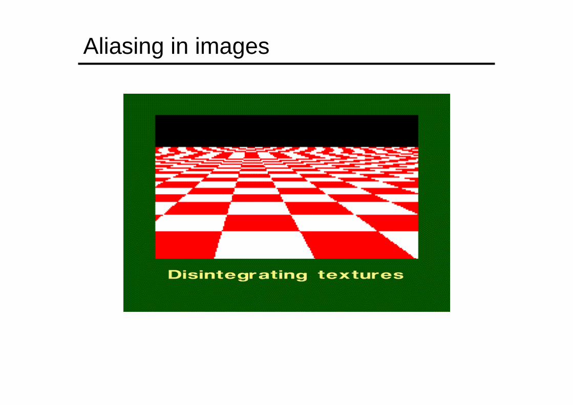
Aliasing in images
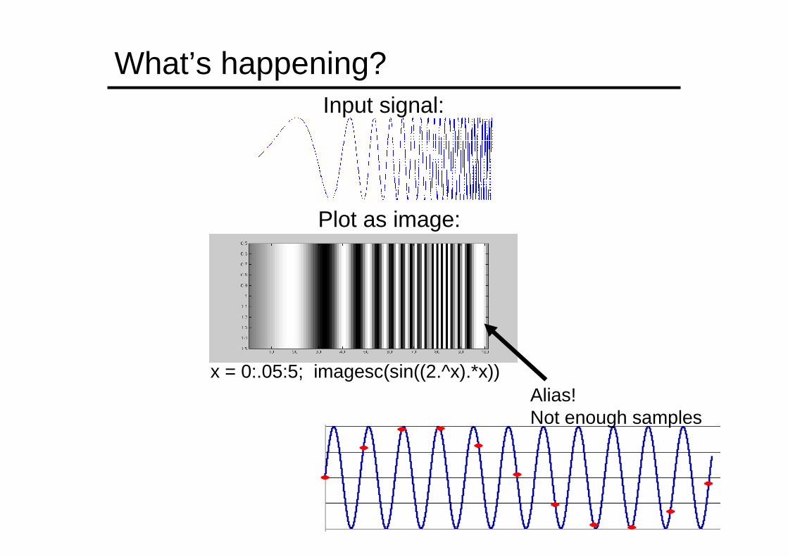
What’s happening?Input signal:
x = 0:.05:5; imagesc(sin((2.^x).*x))
Plot as image:
Alias!Not enough samples
AntialiasingWhat can we do about aliasing?
Sample more often• Join the Mega-Pixel craze of the photo industry• But this can’t go on forever
Make the signal less “wiggly”• Get rid of some high frequencies• Will loose information• But it’s better than aliasing
© 2006 Steve Marschner • 15
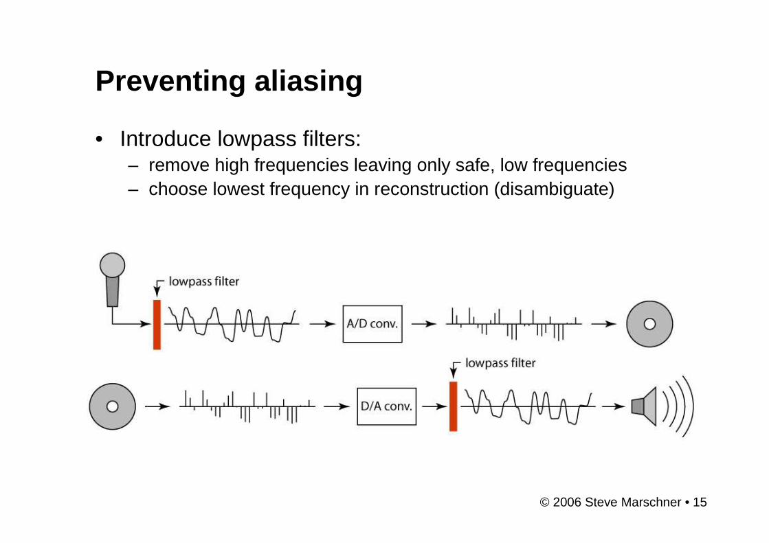
Preventing aliasing
• Introduce lowpass filters:– remove high frequencies leaving only safe, low frequencies– choose lowest frequency in reconstruction (disambiguate)
© 2006 Steve Marschner • 16
Linear filtering: a key idea
• Transformations on signals; e.g.:– bass/treble controls on stereo– blurring/sharpening operations in image editing– smoothing/noise reduction in tracking
• Key properties– linearity: filter(f + g) = filter(f) + filter(g)– shift invariance: behavior invariant to shifting the input
• delaying an audio signal• sliding an image around
• Can be modeled mathematically by convolution
© 2006 Steve Marschner • 17
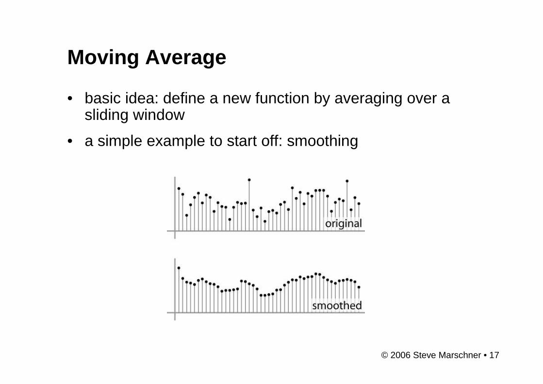
Moving Average
• basic idea: define a new function by averaging over a sliding window
• a simple example to start off: smoothing
© 2006 Steve Marschner • 18
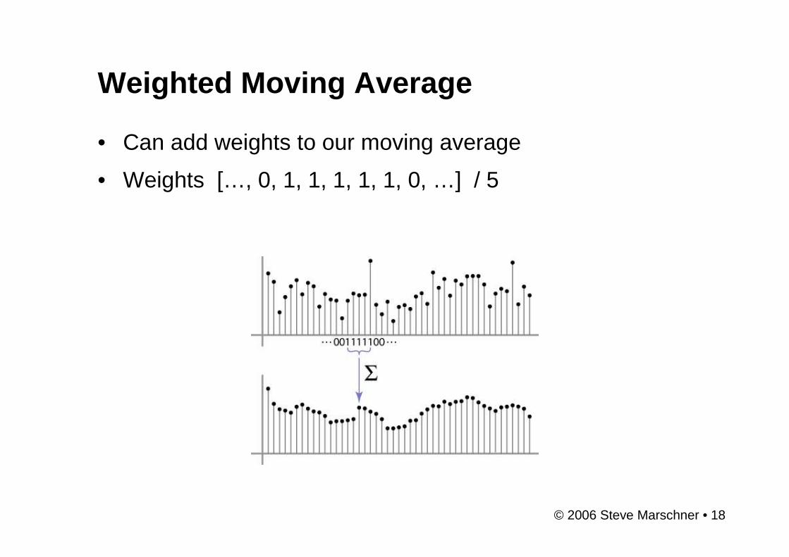
Weighted Moving Average
• Can add weights to our moving average
• Weights […, 0, 1, 1, 1, 1, 1, 0, …] / 5
© 2006 Steve Marschner • 19
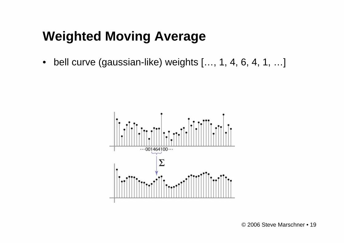
Weighted Moving Average
• bell curve (gaussian-like) weights […, 1, 4, 6, 4, 1, …]
© 2006 Steve Marschner • 20
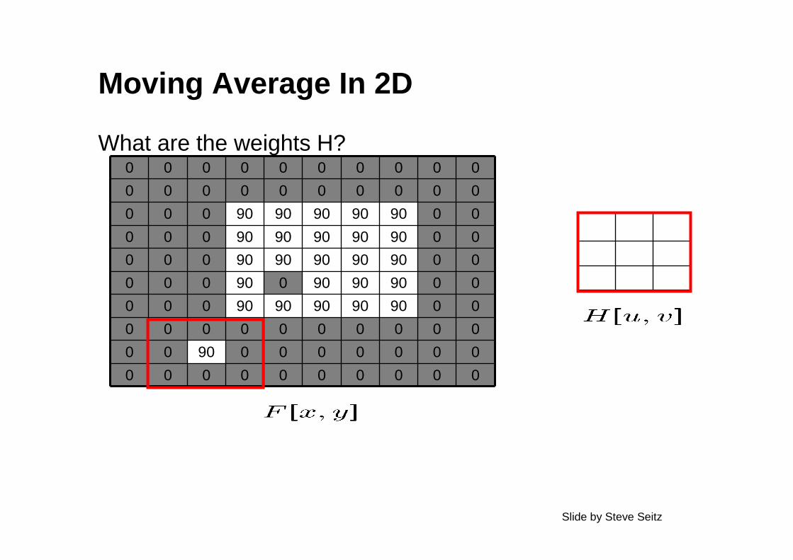
Moving Average In 2D
What are the weights H?0 0 0 0 0 0 0 0 0 0
0 0 0 0 0 0 0 0 0 0
0 0 0 90 90 90 90 90 0 0
0 0 0 90 90 90 90 90 0 0
0 0 0 90 90 90 90 90 0 0
0 0 0 90 0 90 90 90 0 0
0 0 0 90 90 90 90 90 0 0
0 0 0 0 0 0 0 0 0 0
0 0 90 0 0 0 0 0 0 0
0 0 0 0 0 0 0 0 0 0
Slide by Steve Seitz
© 2006 Steve Marschner • 21
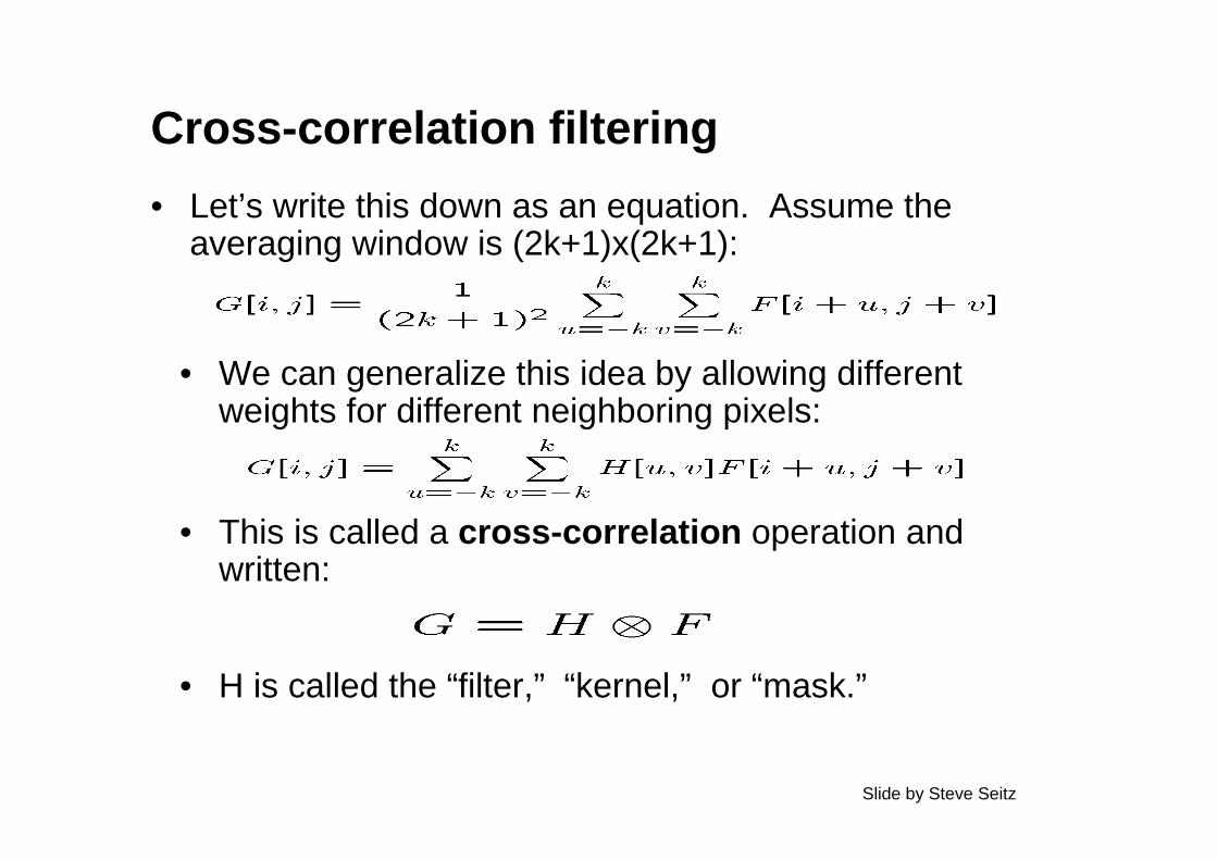
Cross -correlation filtering
• Let’s write this down as an equation. Assume the averaging window is (2k+1)x(2k+1):
• We can generalize this idea by allowing different weights for different neighboring pixels:
• This is called a cross-correlation operation and written:
• H is called the “filter,” “kernel,” or “mask.”
Slide by Steve Seitz
22
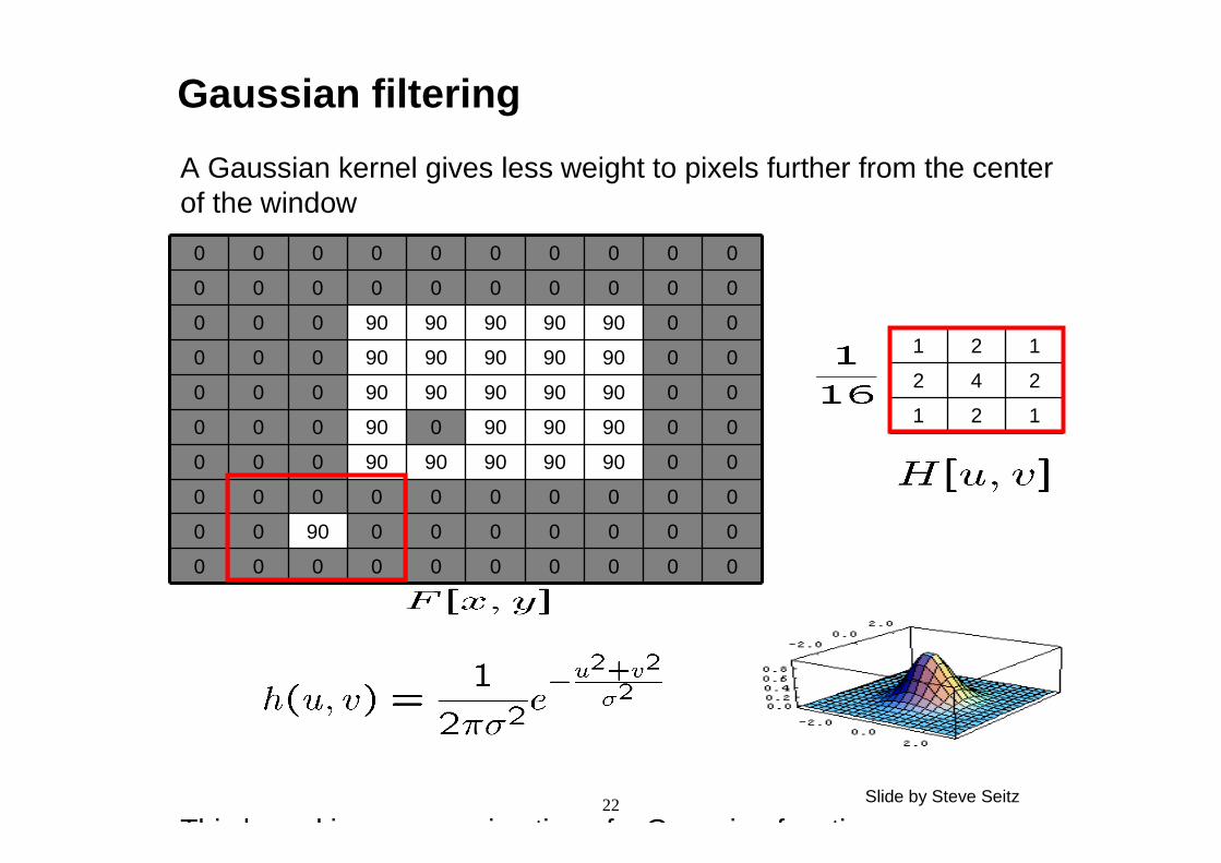
Gaussian filtering
A Gaussian kernel gives less weight to pixels further from the center of the window
This kernel is an approximation of a Gaussian function:
0 0 0 0 0 0 0 0 0 0
0 0 0 0 0 0 0 0 0 0
0 0 0 90 90 90 90 90 0 0
0 0 0 90 90 90 90 90 0 0
0 0 0 90 90 90 90 90 0 0
0 0 0 90 0 90 90 90 0 0
0 0 0 90 90 90 90 90 0 0
0 0 0 0 0 0 0 0 0 0
0 0 90 0 0 0 0 0 0 0
0 0 0 0 0 0 0 0 0 0
1 2 1
2 4 2
1 2 1
Slide by Steve Seitz
23
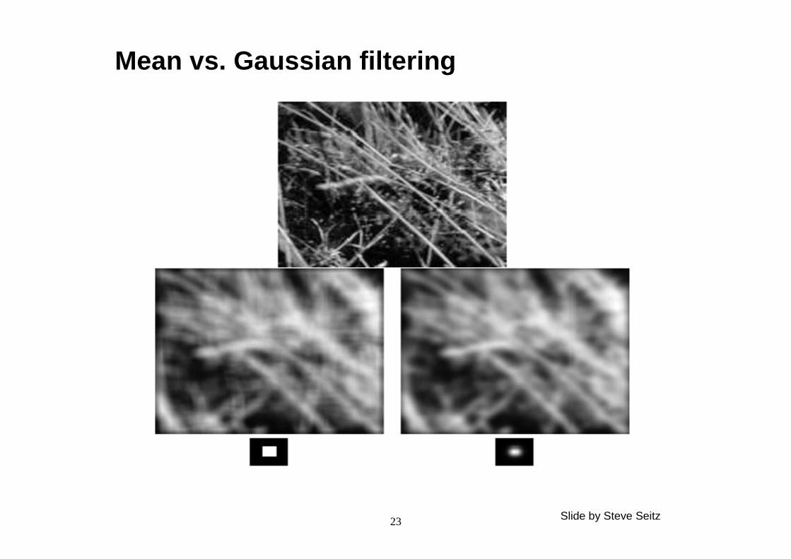
Mean vs. Gaussian filtering
Slide by Steve Seitz
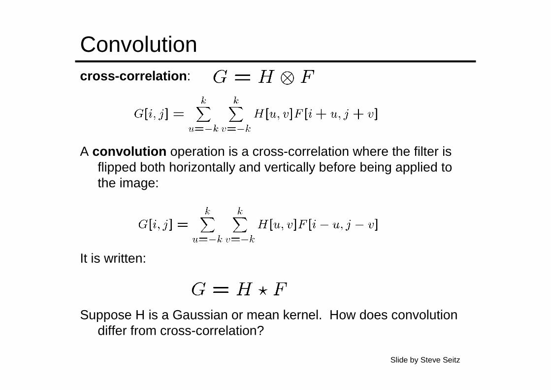
Convolutioncross-correlation :
A convolution operation is a cross-correlation where the filter is flipped both horizontally and vertically before being applied tothe image:
It is written:
Suppose H is a Gaussian or mean kernel. How does convolution differ from cross-correlation?
Slide by Steve Seitz
© 2006 Steve Marschner • 25
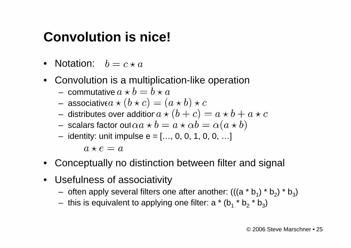
Convolution is nice!
• Notation:
• Convolution is a multiplication-like operation– commutative– associative– distributes over addition– scalars factor out– identity: unit impulse e = […, 0, 0, 1, 0, 0, …]
• Conceptually no distinction between filter and signal
• Usefulness of associativity– often apply several filters one after another: (((a * b1) * b2) * b3)– this is equivalent to applying one filter: a * (b1 * b2 * b3)
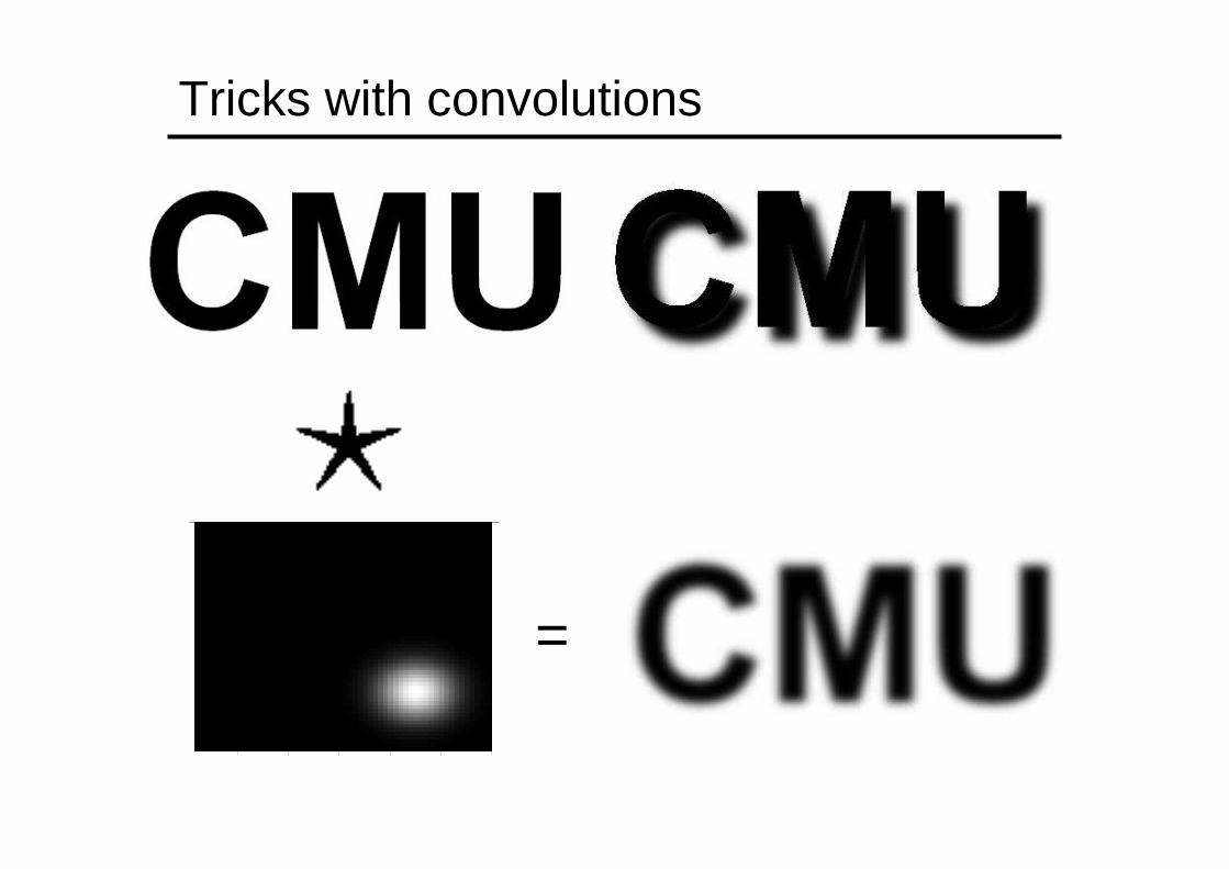
Tricks with convolutions
=
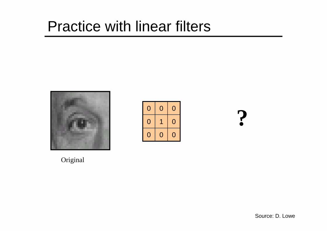
Practice with linear filters
000
010
000
Original
?
Source: D. Lowe
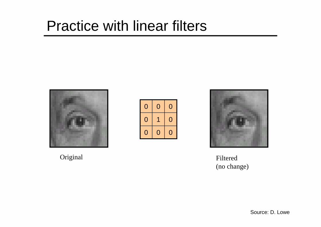
Practice with linear filters
000
010
000
Original Filtered (no change)
Source: D. Lowe

Practice with linear filters
000
100
000
Original
?
Source: D. Lowe
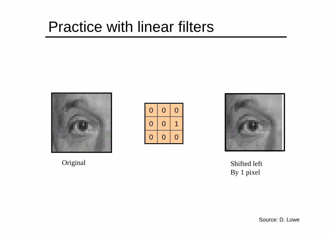
Practice with linear filters
000
100
000
Original Shifted leftBy 1 pixel
Source: D. Lowe
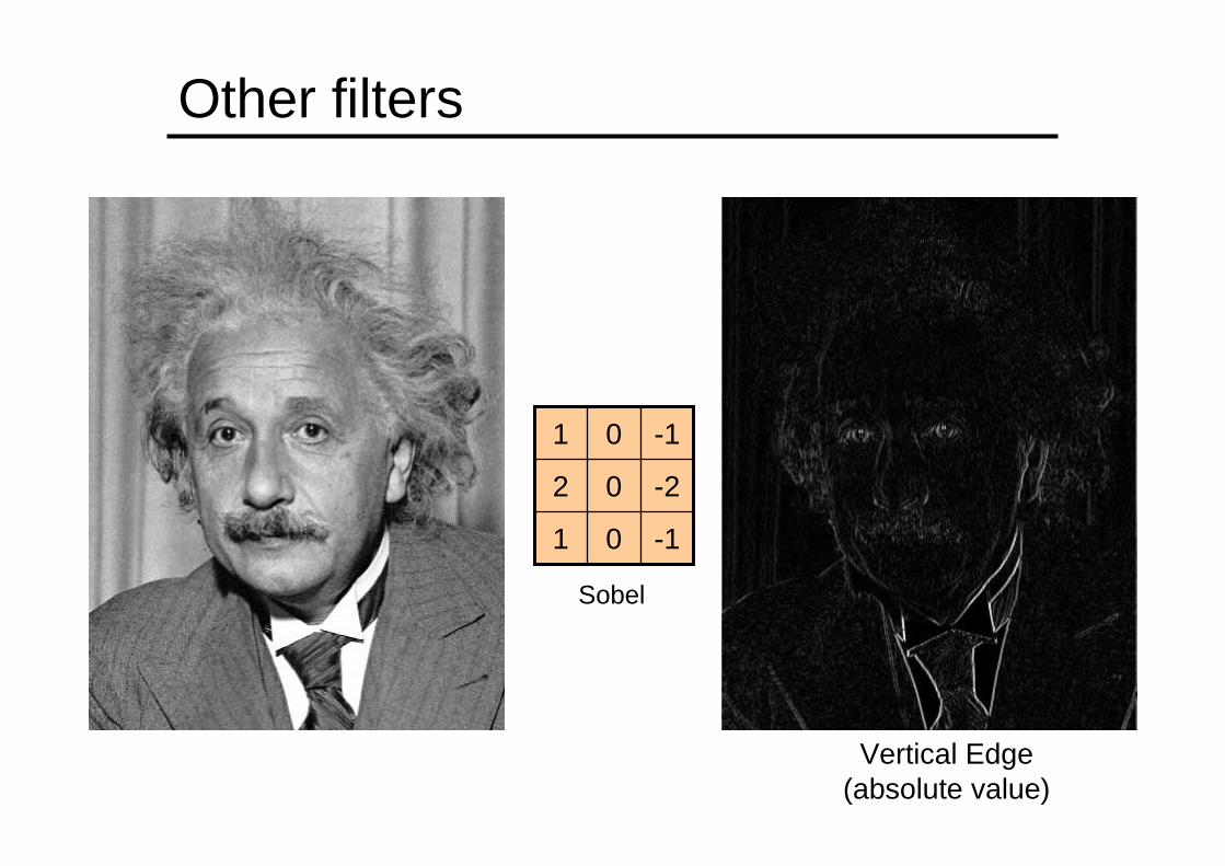
Other filters
-101
-202
-101
Vertical Edge(absolute value)
Sobel

Other filters
-1-2-1
000
121
Horizontal Edge(absolute value)
Sobel
Q?
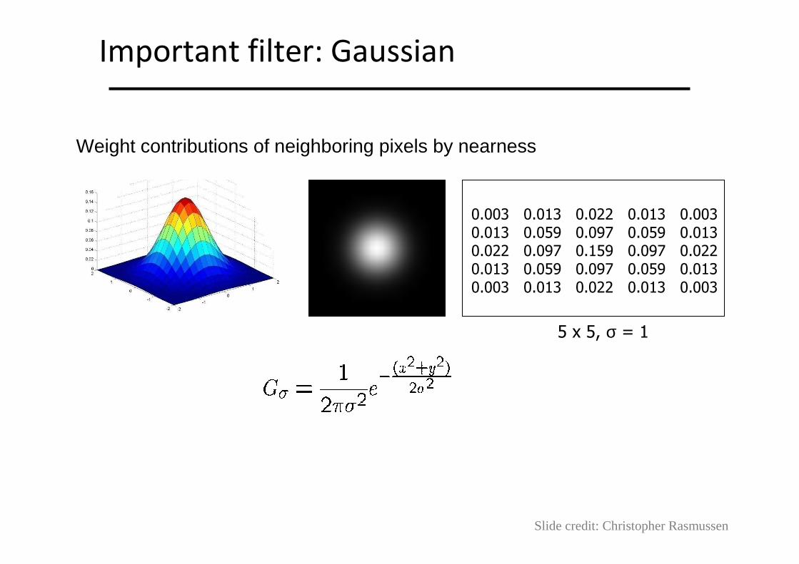
Weight contributions of neighboring pixels by nearness
0.003 0.013 0.022 0.013 0.003
0.013 0.059 0.097 0.059 0.013
0.022 0.097 0.159 0.097 0.022
0.013 0.059 0.097 0.059 0.013
0.003 0.013 0.022 0.013 0.003
5 x 5, σ = 1
Slide credit: Christopher Rasmussen
Important filter: Gaussian
Gaussian filters
Remove “high-frequency” components from the image (low-pass filter)• Images become more smooth
Convolution with self is another Gaussian• So can smooth with small-width kernel, repeat, and get
same result as larger-width kernel would have• Convolving two times with Gaussian kernel of width σ is
same as convolving once with kernel of width σ√2
Source: K. Grauman
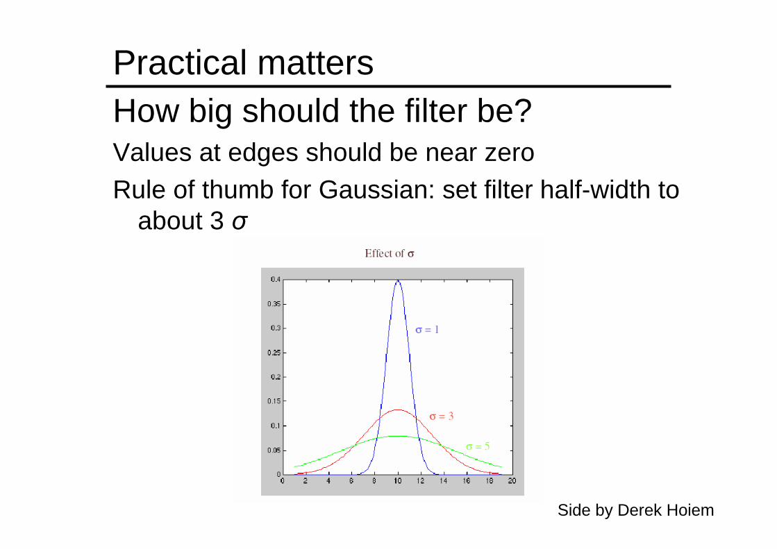
How big should the filter be?Values at edges should be near zero
Rule of thumb for Gaussian: set filter half-width to about 3 σ
Practical matters
Side by Derek Hoiem
Practical matters
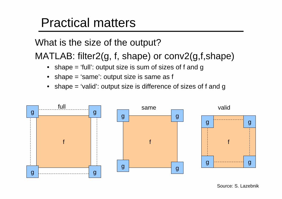
What is the size of the output?
MATLAB: filter2(g, f, shape) or conv2(g,f,shape)• shape = ‘full’: output size is sum of sizes of f and g• shape = ‘same’: output size is same as f• shape = ‘valid’: output size is difference of sizes of f and g
f
gg
gg
f
gg
gg
f
gg
gg
full same valid
Source: S. Lazebnik
Practical matters
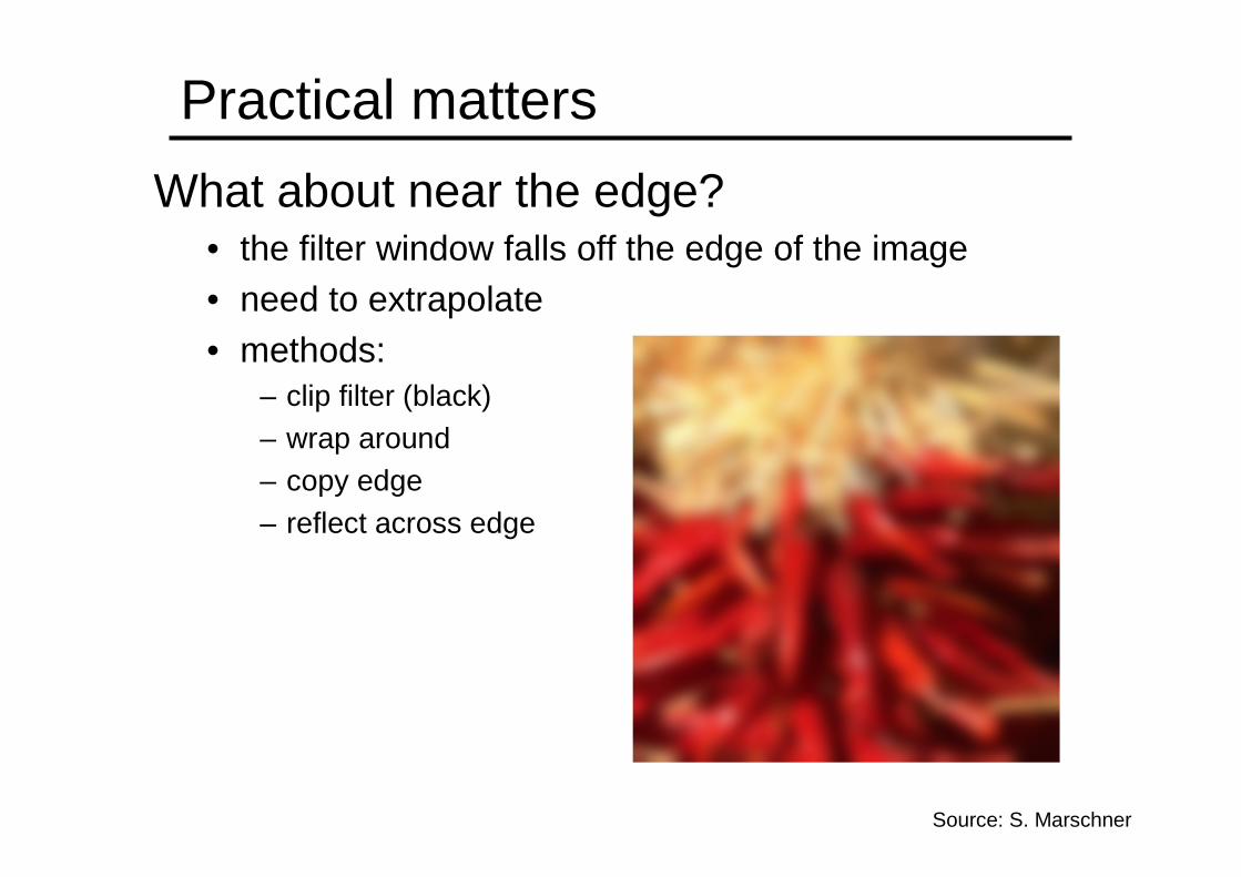
What about near the edge?• the filter window falls off the edge of the image• need to extrapolate• methods:
– clip filter (black)– wrap around– copy edge– reflect across edge
Source: S. Marschner
Practical matters
• methods (MATLAB):– clip filter (black): imfilter(f, g, 0)– wrap around: imfilter(f, g, ‘circular’)– copy edge: imfilter(f, g, ‘replicate’)– reflect across edge: imfilter(f, g, ‘symmetric’)
Source: S. Marschner
Q?
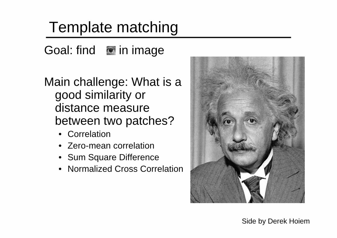
Template matchingGoal: find in image
Main challenge: What is a good similarity or distance measure between two patches?• Correlation• Zero-mean correlation• Sum Square Difference• Normalized Cross Correlation
Side by Derek Hoiem
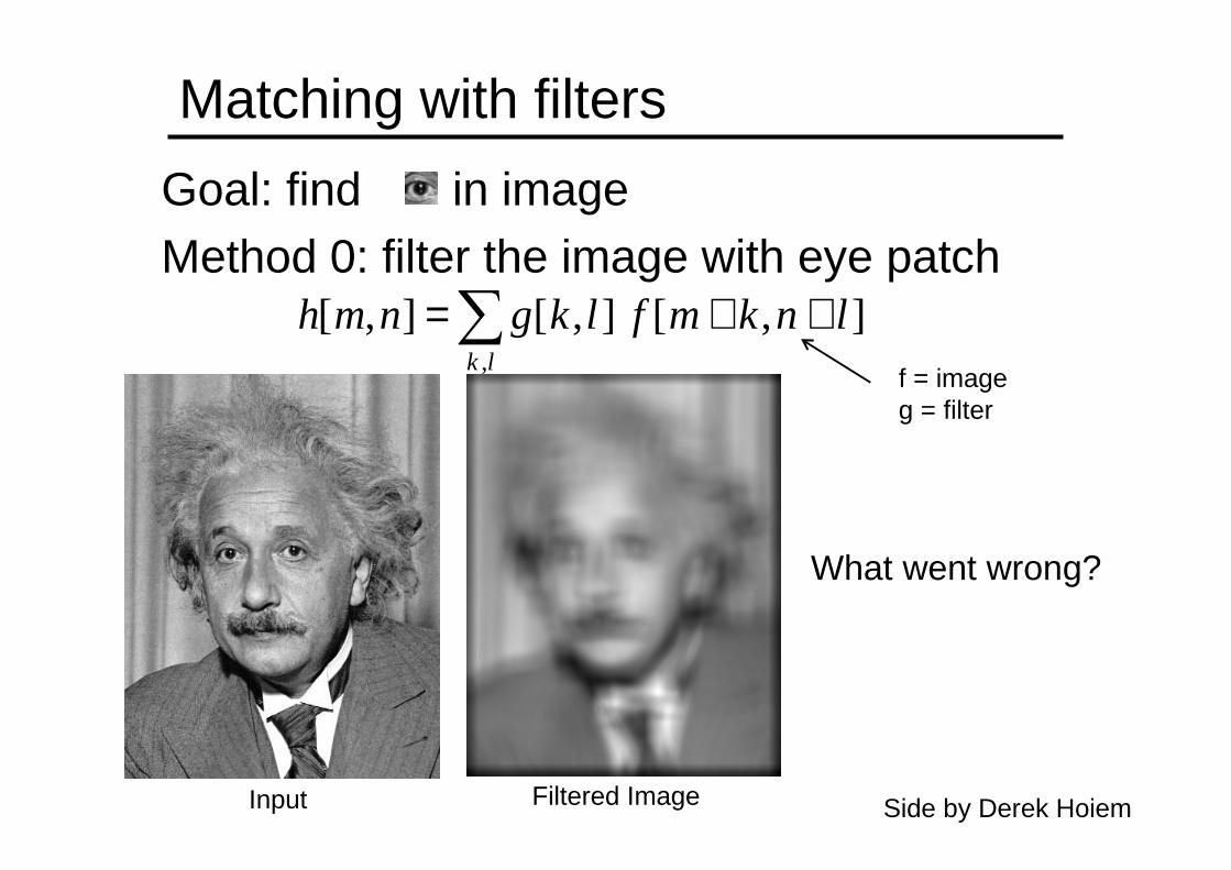
Matching with filters
Goal: find in imageMethod 0: filter the image with eye patch
Input Filtered Image
],[],[],[,
lnkmflkgnmhlk
++=∑
What went wrong?
f = imageg = filter
Side by Derek Hoiem
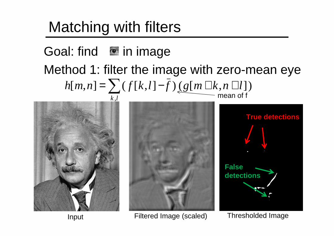
Matching with filters
Goal: find in imageMethod 1: filter the image with zero-mean eye
Input Filtered Image (scaled) Thresholded Image
)],[()],[(],[,
lnkmgflkfnmhlk
++−=∑
True detections
False detections
mean of f
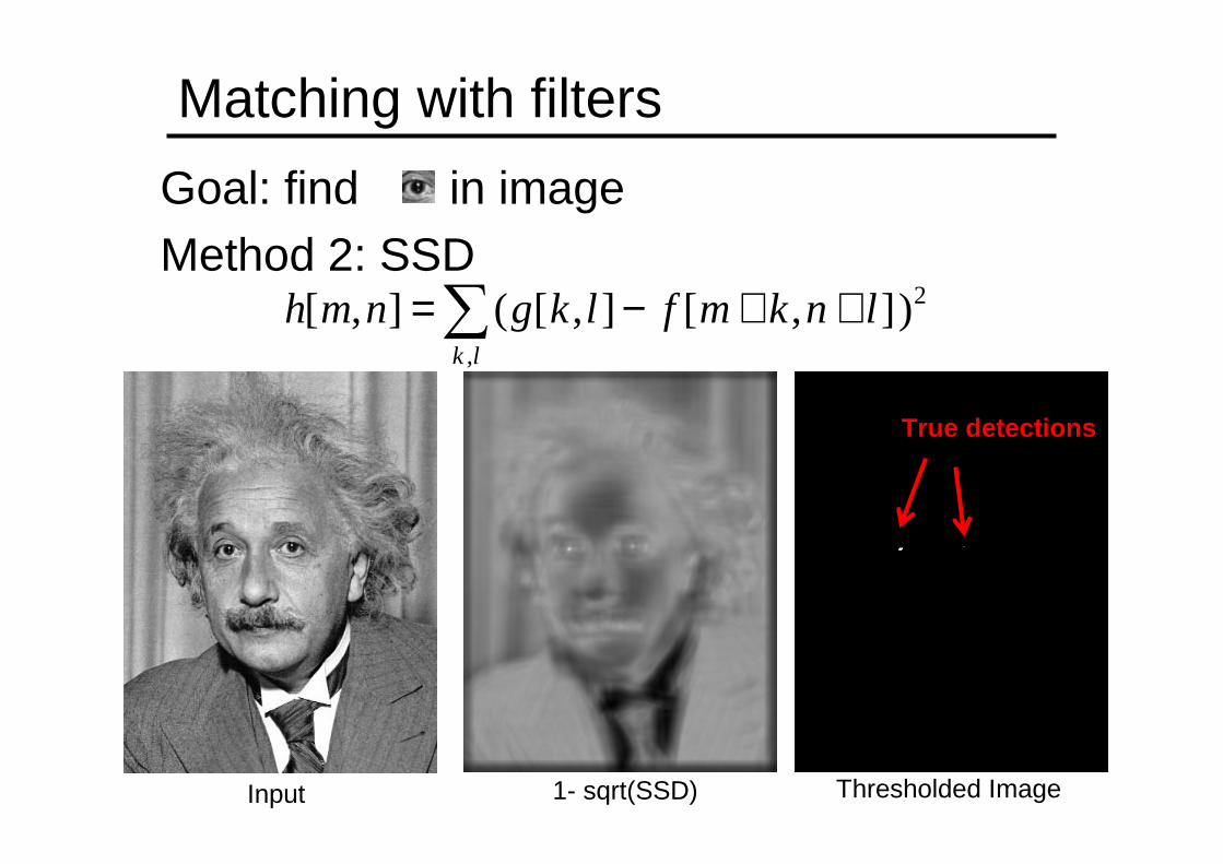
Matching with filters
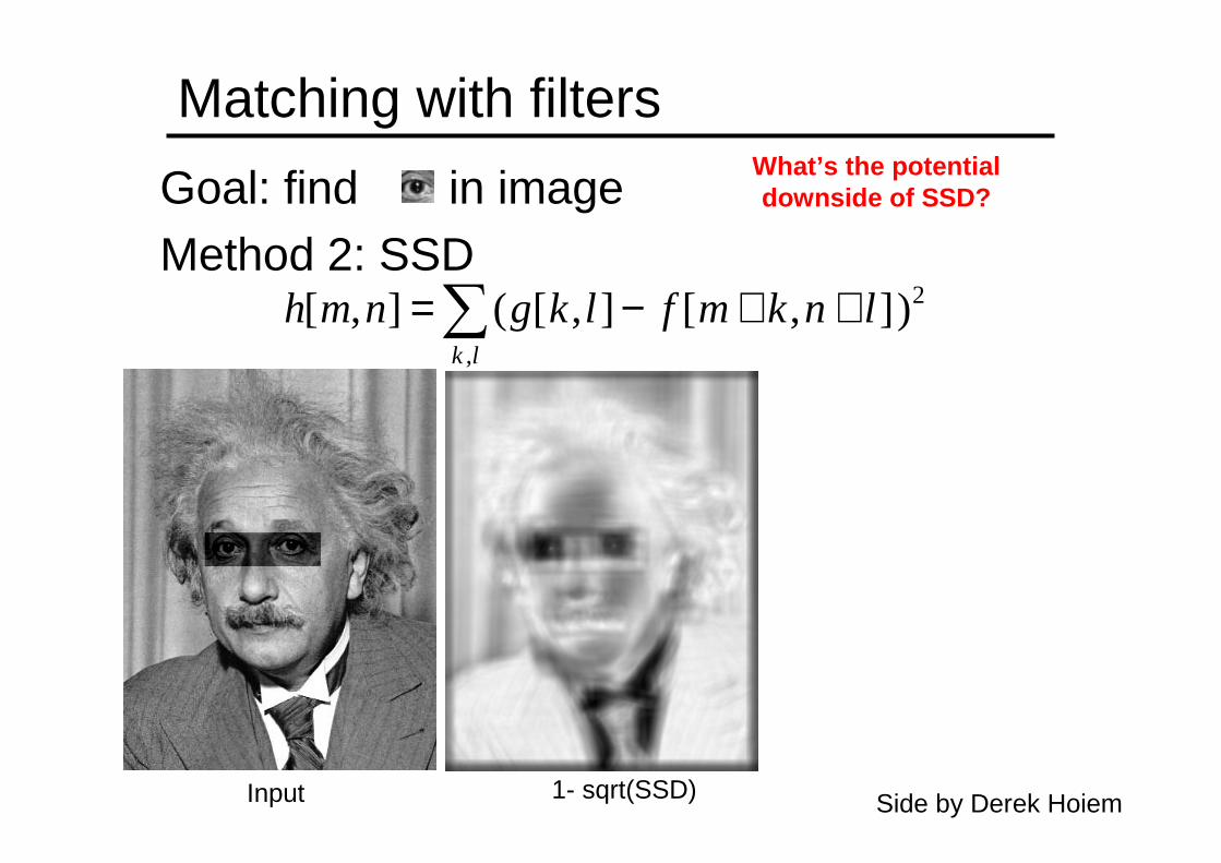
Goal: find in imageMethod 2: SSD
Input 1- sqrt(SSD) Thresholded Image
2
,
)],[],[(],[ lnkmflkgnmhlk
++−=∑
True detections
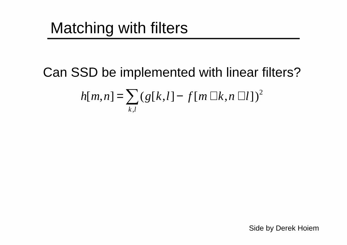
Matching with filters
Can SSD be implemented with linear filters?2
,
)],[],[(],[ lnkmflkgnmhlk
++−=∑
Side by Derek Hoiem
Matching with filters
Goal: find in imageMethod 2: SSD
Input 1- sqrt(SSD)
2
,
)],[],[(],[ lnkmflkgnmhlk
++−=∑
What’s the potential downside of SSD?
Side by Derek Hoiem

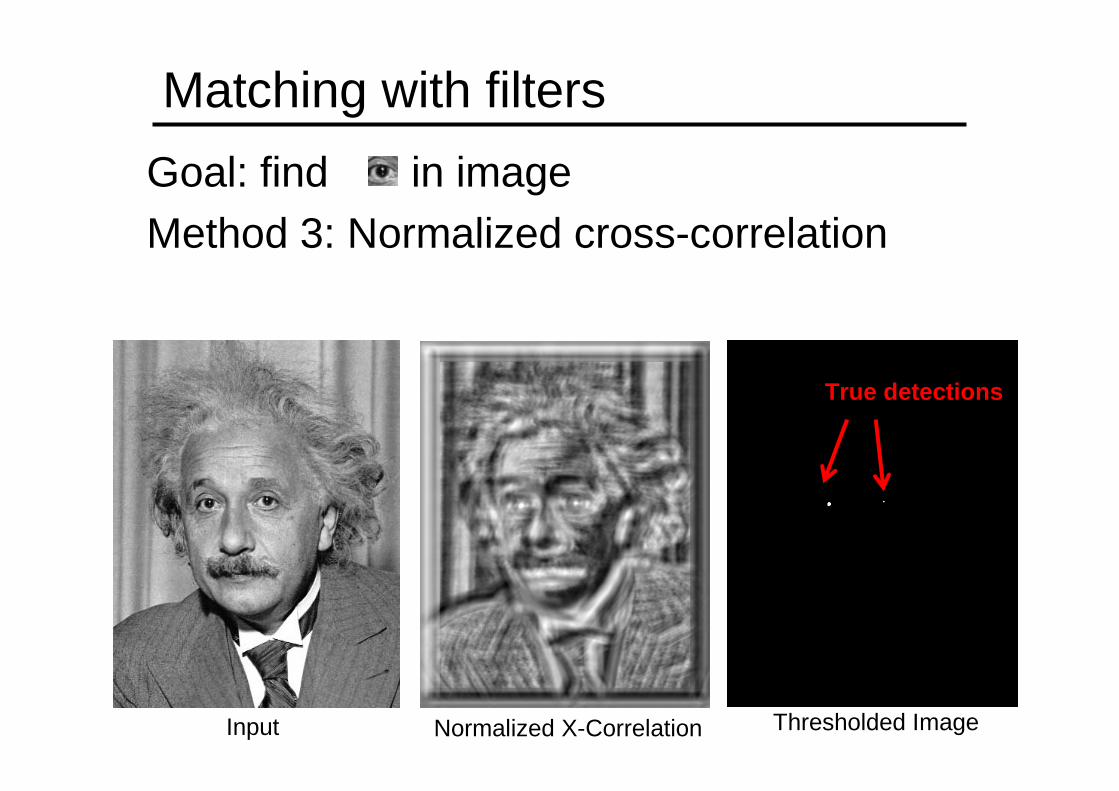
Matching with filters
Goal: find in imageMethod 3: Normalized cross-correlation
5.0
,
2,
,
2
,,
)],[()],[(
)],[)(],[(
],[
−++−
−++−=
∑ ∑
∑
lknm
lk
nmlk
flnkmfglkg
flnkmfglkg
nmh
mean image patchmean template
Side by Derek Hoiem
Matching with filters
Goal: find in imageMethod 3: Normalized cross-correlation
Input Normalized X-Correlation Thresholded Image
True detections
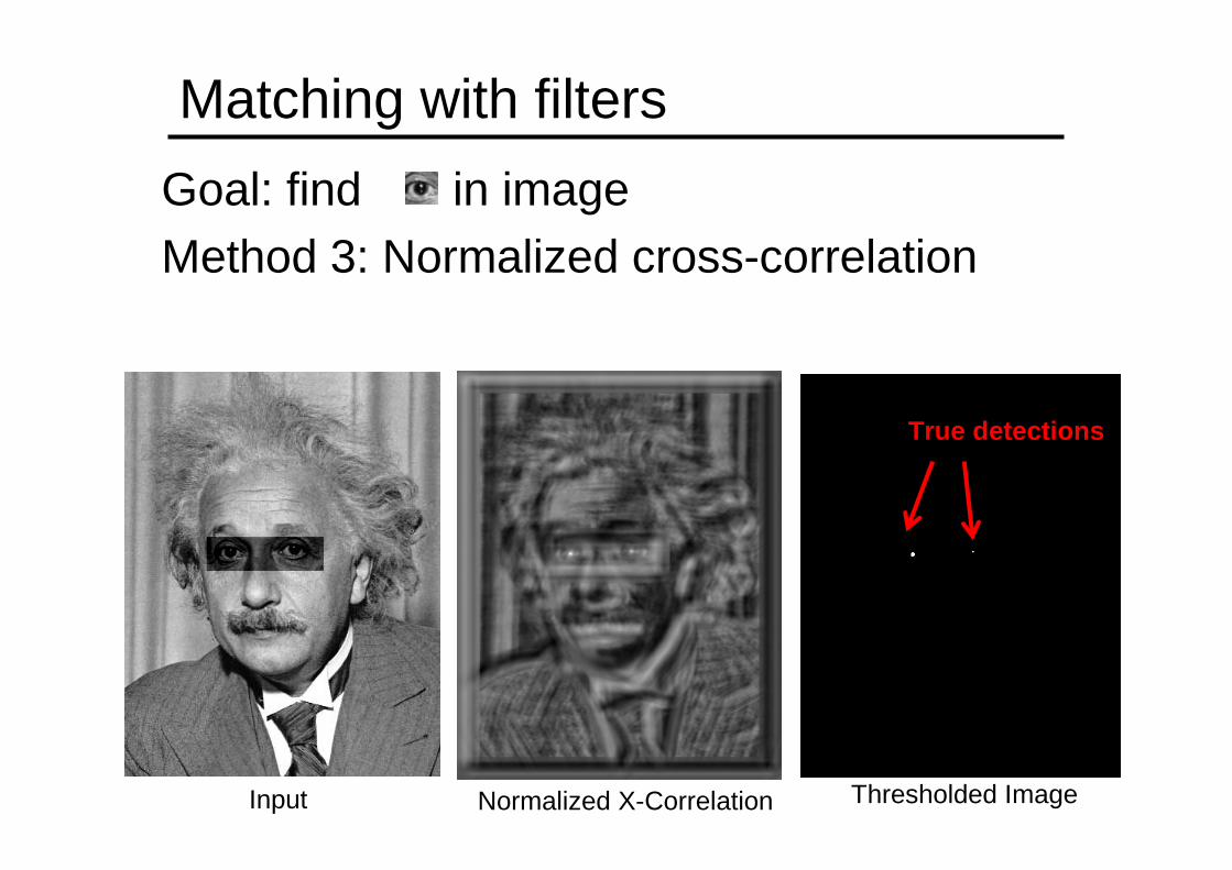
Matching with filters
Goal: find in imageMethod 3: Normalized cross-correlation
Input Normalized X-Correlation Thresholded Image
True detections
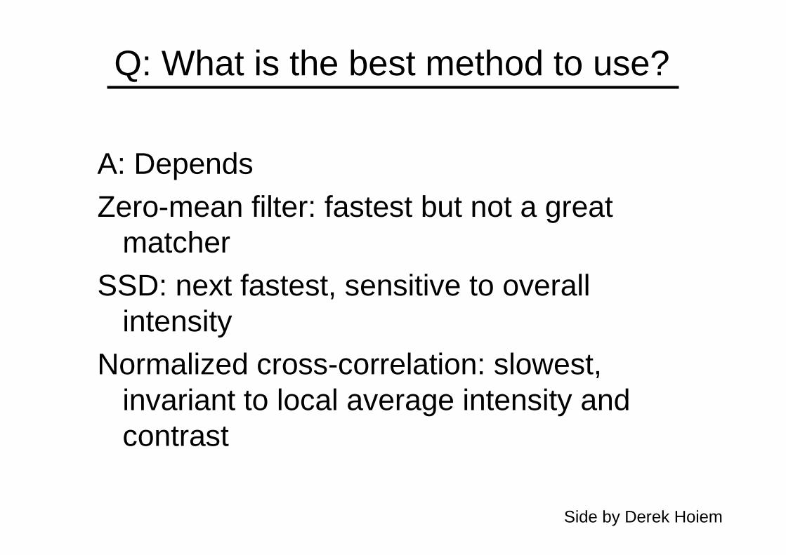
Q: What is the best method to use?
A: DependsZero-mean filter: fastest but not a great
matcherSSD: next fastest, sensitive to overall
intensityNormalized cross-correlation: slowest,
invariant to local average intensity and contrast
Side by Derek Hoiem
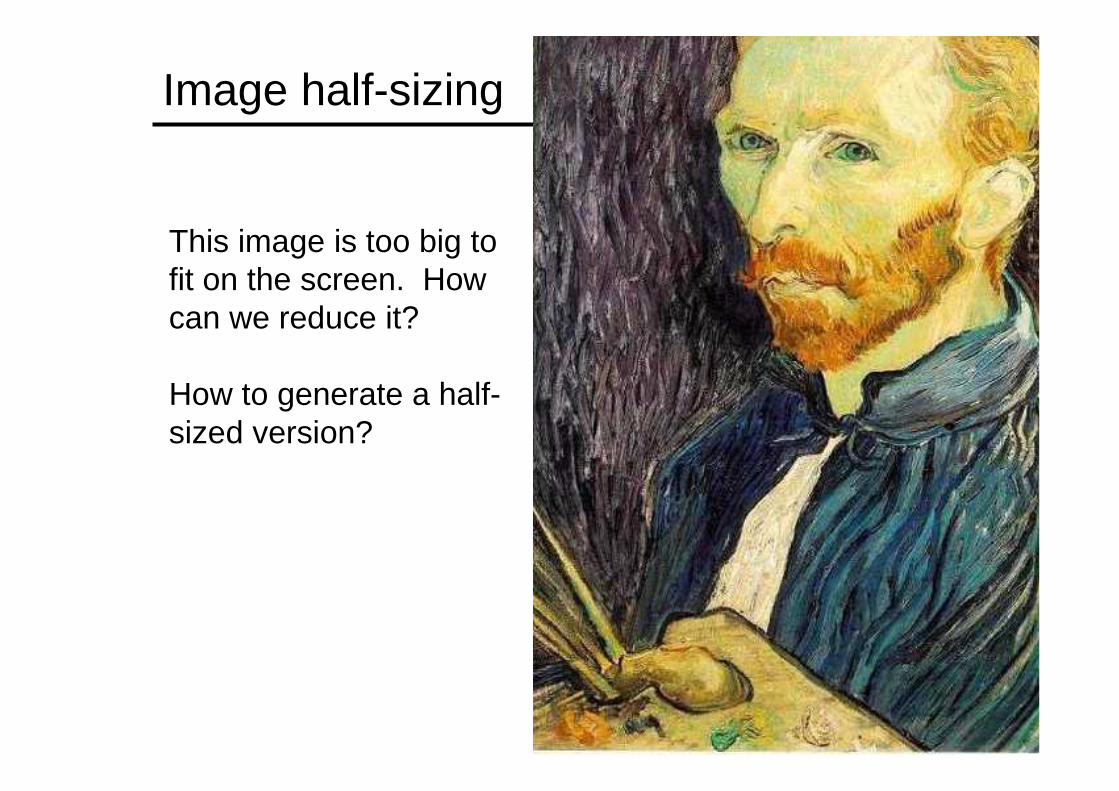
Image half-sizing
This image is too big tofit on the screen. Howcan we reduce it?
How to generate a half-sized version?
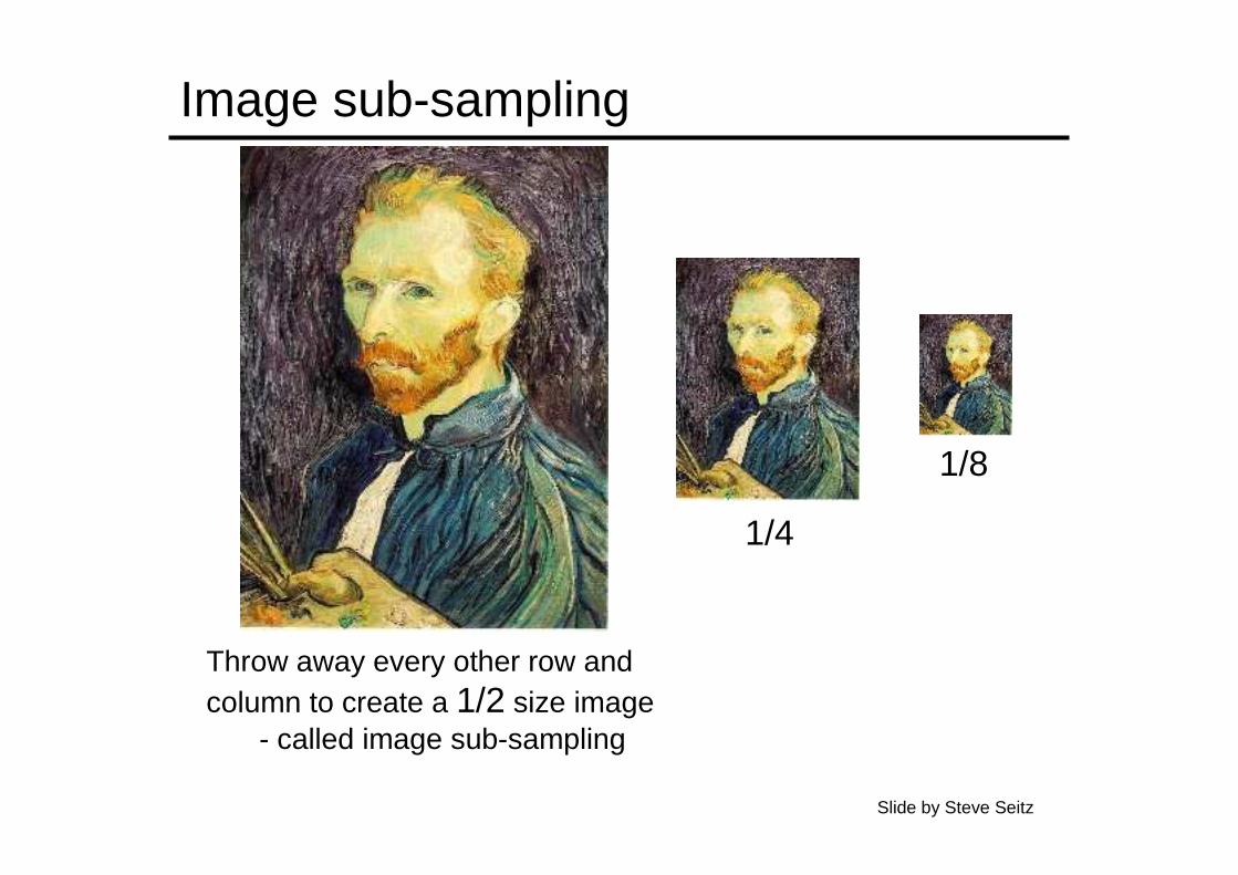
Image sub-sampling
Throw away every other row and column to create a 1/2 size image
- called image sub-sampling
1/4
1/8
Slide by Steve Seitz

Image sub-sampling
1/4 (2x zoom) 1/8 (4x zoom)
Aliasing! What do we do?
1/2
Slide by Steve Seitz

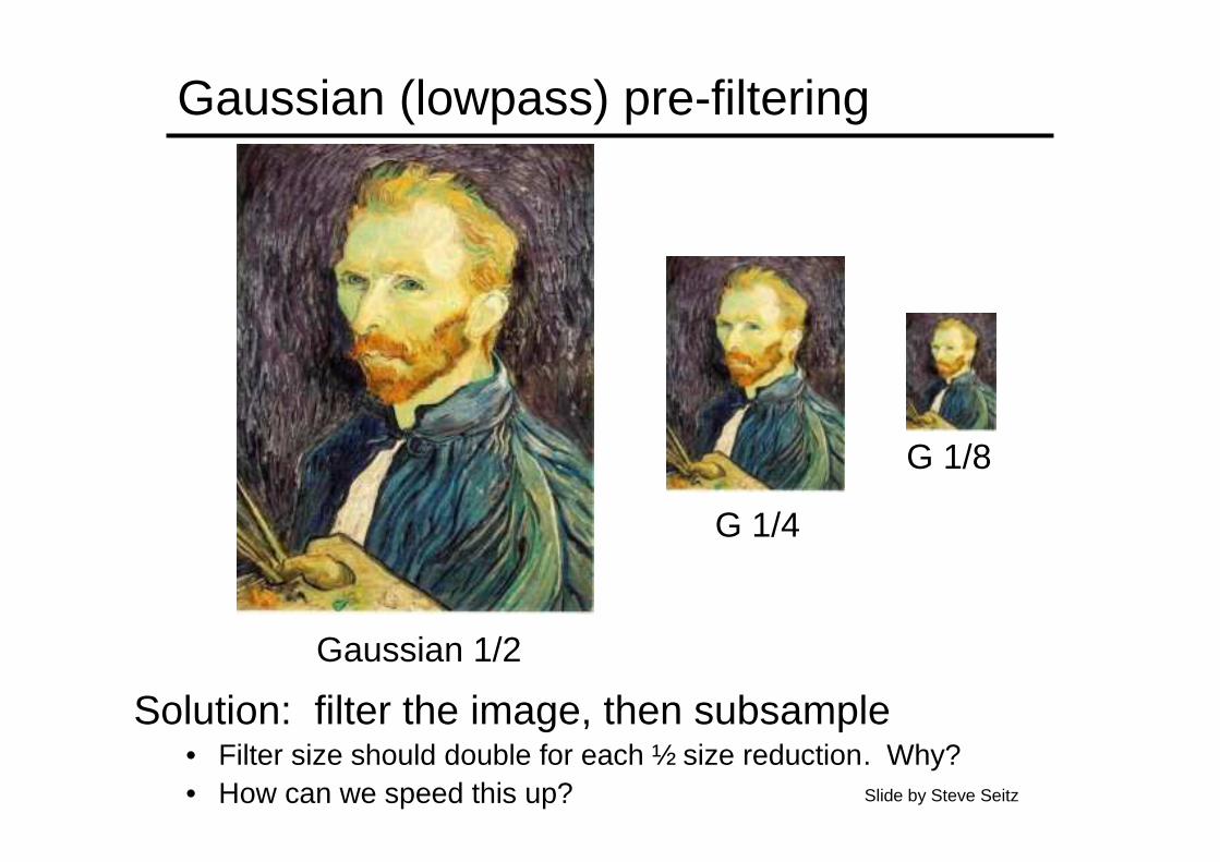
Gaussian (lowpass) pre-filtering
G 1/4
G 1/8
Gaussian 1/2
Solution: filter the image, then subsample• Filter size should double for each ½ size reduction. Why?
Slide by Steve Seitz
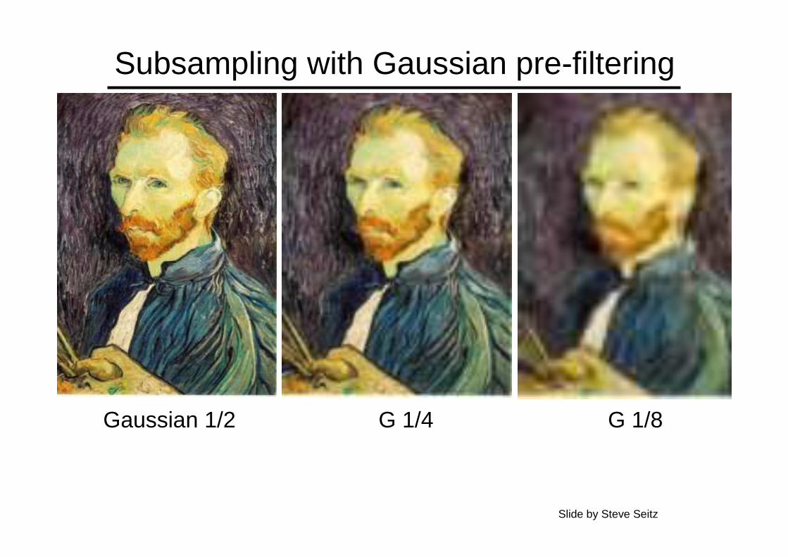
Subsampling with Gaussian pre-filtering
G 1/4 G 1/8Gaussian 1/2
Slide by Steve Seitz
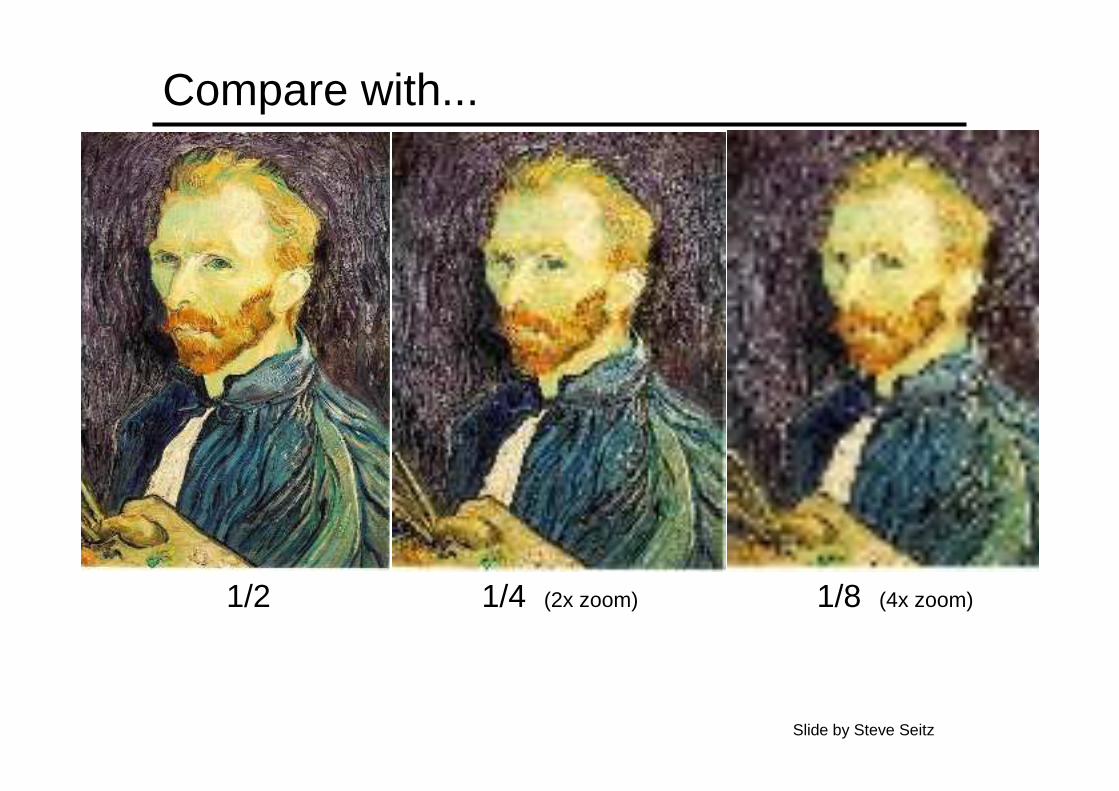
Compare with...
1/4 (2x zoom) 1/8 (4x zoom)1/2
Slide by Steve Seitz
Gaussian (lowpass) pre-filtering
G 1/4
G 1/8
Gaussian 1/2
Solution: filter the image, then subsample• Filter size should double for each ½ size reduction. Why?• How can we speed this up? Slide by Steve Seitz
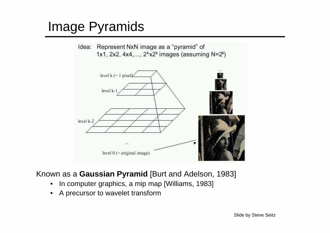
Image Pyramids
Known as a Gaussian Pyramid [Burt and Adelson, 1983]• In computer graphics, a mip map [Williams, 1983]• A precursor to wavelet transform
Slide by Steve Seitz
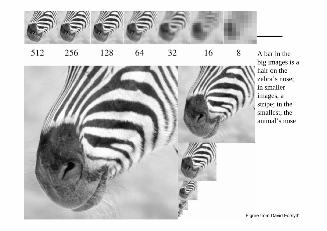
A bar in the big images is a hair on the zebra’s nose; in smaller images, a stripe; in the smallest, the animal’s nose
Figure from David Forsyth
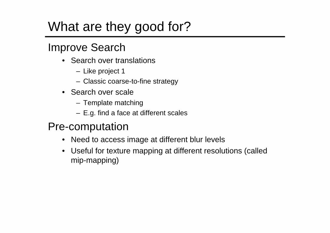
What are they good for?
Improve Search• Search over translations
– Like project 1– Classic coarse-to-fine strategy
• Search over scale– Template matching– E.g. find a face at different scales
Pre-computation• Need to access image at different blur levels• Useful for texture mapping at different resolutions (called
mip-mapping)
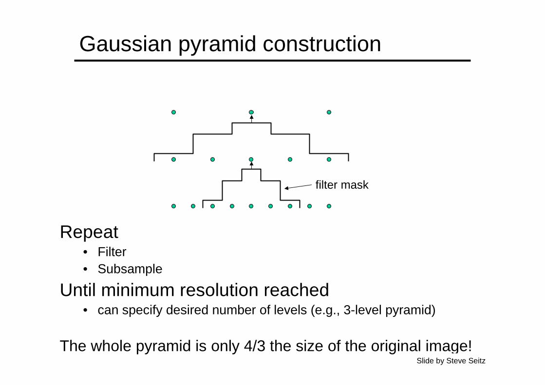
Gaussian pyramid construction
filter mask
Repeat• Filter• Subsample
Until minimum resolution reached • can specify desired number of levels (e.g., 3-level pyramid)
The whole pyramid is only 4/3 the size of the original image!Slide by Steve Seitz
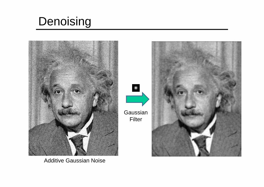
Denoising
Additive Gaussian Noise
Gaussian Filter
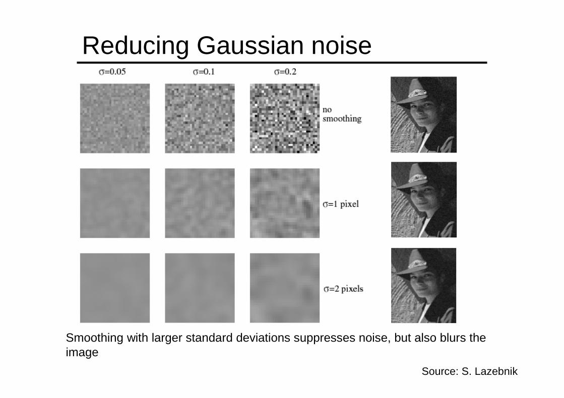
Smoothing with larger standard deviations suppresses noise, but also blurs the image
Reducing Gaussian noise
Source: S. Lazebnik
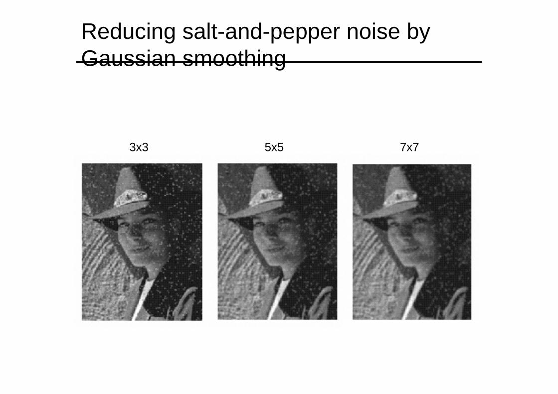
Reducing salt-and-pepper noise by Gaussian smoothing
3x3 5x5 7x7
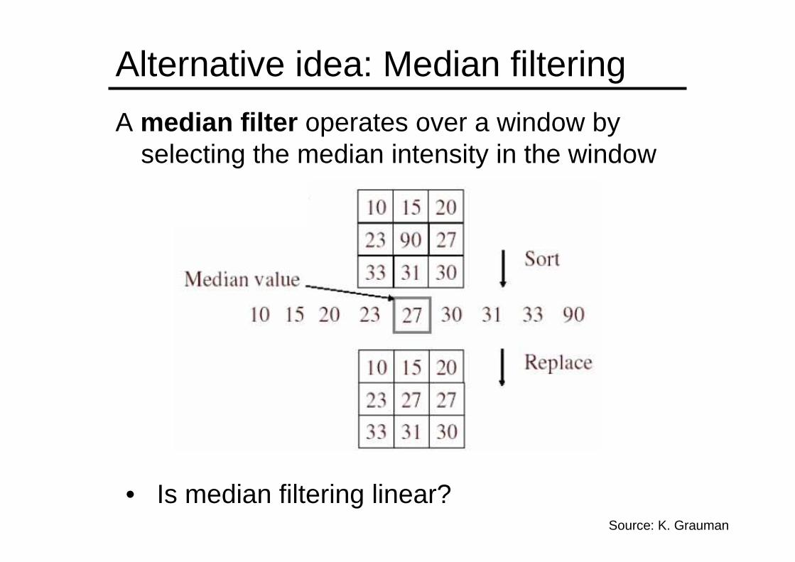
Alternative idea: Median filtering
A median filter operates over a window by selecting the median intensity in the window
• Is median filtering linear?Source: K. Grauman
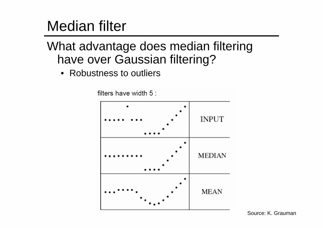
Median filterWhat advantage does median filtering
have over Gaussian filtering?• Robustness to outliers
Source: K. Grauman
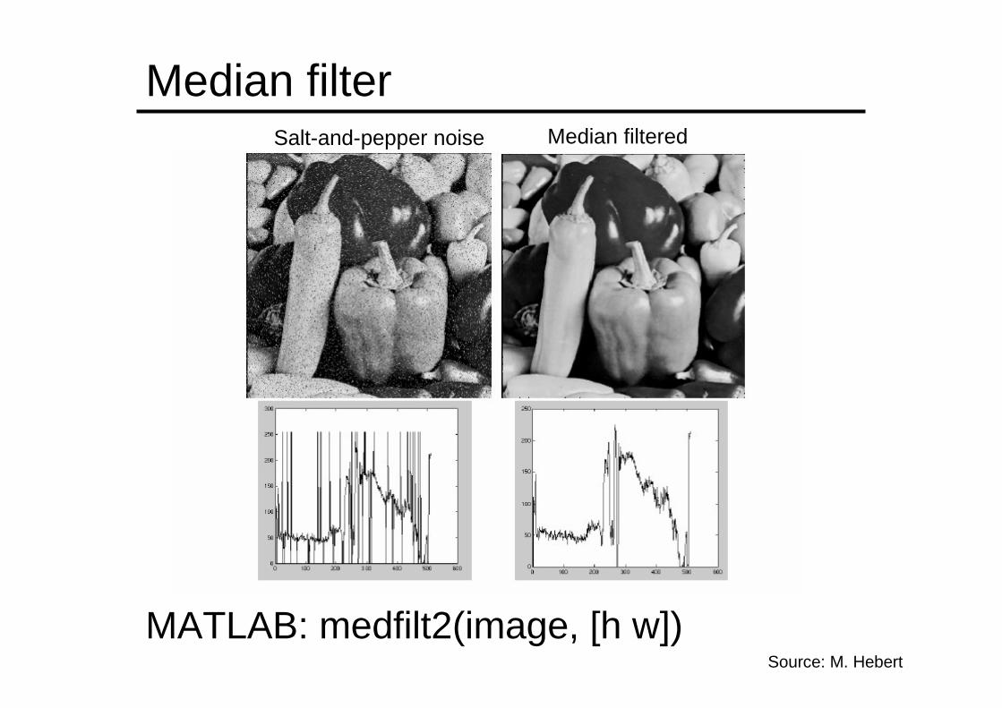
Median filterSalt-and-pepper noise Median filtered
Source: M. Hebert
MATLAB: medfilt2(image, [h w])
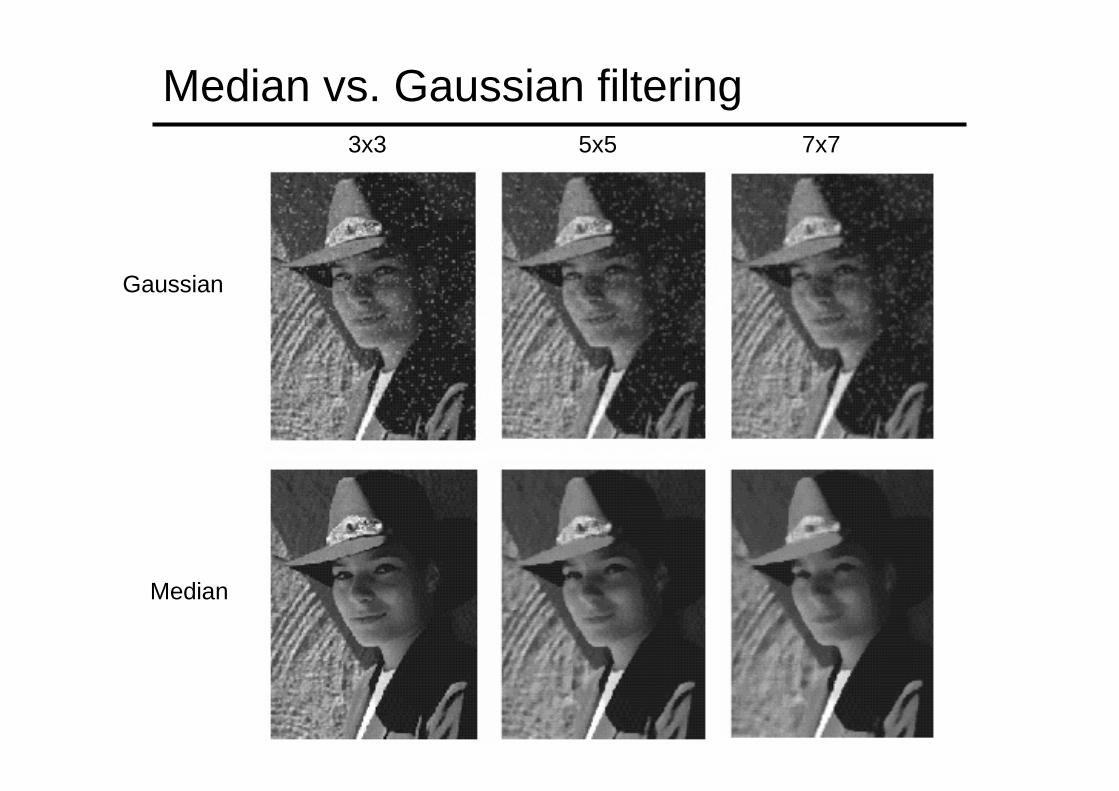
Median vs. Gaussian filtering3x3 5x5 7x7
Gaussian
Median