sampling-based query...

Sampling-Based Query Re-Optimization

Wentao Wu Jeffrey F. Naughton Harneet SinghDepartment of Computer Sciences, University of Wisconsin-Madison

{wentaowu, naughton, harneet}@cs.wisc.edu

ABSTRACTDespite of decades of work, query optimizers still make mistakeson “difficult” queries because of bad cardinality estimates, oftendue to the interaction of multiple predicates and correlations in thedata. In this paper, we propose a low-cost post-processing step thatcan take a plan produced by the optimizer, detect when it is likelyto have made such a mistake, and take steps to fix it. Specifically,our solution is a sampling-based iterative procedure that requiresalmost no changes to the original query optimizer or query evalua-tion mechanism of the system. We show that this indeed imposeslow overhead and catches cases where three widely used optimizers(PostgreSQL and two commercial systems) make large errors.

1. INTRODUCTIONQuery optimizers rely on decent cost estimates of query plans.

Cardinality/selectivity estimation is crucial for the accuracy of costestimates. Unfortunately, although decades of research has beendevoted to this area and significant progress has been made, cardi-nality estimation remains challenging. In current database systems,the dominant approach is to keep various statistics, primarily his-tograms, about the data. While histogram-based approaches haveworked well for estimating selectivities of local predicates (i.e.,predicates over a column of a base table), query optimizers stillmake mistakes on “difficult” queries, often due to the interaction ofmultiple predicates and correlations in the data [28].

Indeed, there is a great deal of work in the literature explor-ing selectivity estimation techniques beyond histogram-based ones(see Section 6). Nonetheless, histogram-based approaches remaindominant in practice because of its low overhead. Note that, queryoptimizers may explore hundreds or even thousands of candidateswhen searching for an optimal query plan, and selectivity estima-tion needs to be done for each candidate. As a result, a feasiblesolution has to improve cardinality estimation quality without sig-nificantly increasing query optimization time.

In this paper, we propose a low-cost post-processing step thatcan take a plan produced by the optimizer, detect when it is likelyto have made such a mistake, and take steps to fix it. Specifically,our solution is a sampling-based iterative procedure that requires

Permission to make digital or hard copies of all or part of this work for personal orclassroom use is granted without fee provided that copies are not made or distributedfor profit or commercial advantage and that copies bear this notice and the full cita-tion on the first page. Copyrights for components of this work owned by others thanACM must be honored. Abstracting with credit is permitted. To copy otherwise, or re-publish, to post on servers or to redistribute to lists, requires prior specific permissionand/or a fee. Request permissions from [email protected].

SIGMOD’16, June 26-July 01, 2016, San Francisco, CA, USAc© 2016 ACM. ISBN 978-1-4503-3531-7/16/06. . . $15.00

DOI: http://dx.doi.org/10.1145/2882903.2882914

almost no changes to the original query optimizer or query evalua-tion mechanism of the system. We show that this indeed imposeslow overhead and catches cases where three widely used optimizers(PostgreSQL and two commercial systems) make large errors.

In more detail, sampling-based approaches (e.g., [11, 20, 27])automatically reflect correlation in the data and between multiplepredicates over the data, so they can provide better cardinality es-timates on correlated data than histogram-based approaches. How-ever, sampling also incurs higher overhead. In previous work [39,40, 41], the authors investigated the effectiveness of using sampling-based cardinality estimates to get better query running time predic-tions. The key observation is the following: while it is infeasibleto use sampling for all plans explored by the optimizer, it is feasi-ble to use sampling as a “post-processing” step after the search isfinished to detect potential errors in optimizer’s original cardinalityestimates for the final chosen plan.

Inspired by this observation, our basic idea is simple: if signifi-cant cardinality estimation errors are detected, the optimality of thereturned plan is then itself questionable, so we go one step furtherto let the optimizer re-optimize the query by also feeding it the car-dinality estimates refined via sampling. This gives the optimizersecond chance to generate a different, perhaps better, plan. Notethat we can again apply the sampling-based validation step to thisnew plan returned by the optimizer. It therefore leads to an iter-ative procedure based on feedback from sampling: we can repeatthis optimization-then-validation loop until the plan chosen by theoptimizer does not change. The hope is that this re-optimizationprocedure can catch large optimizer errors before the system evenbegins executing the chosen query plan.

A couple of natural concerns arise regarding this simple queryre-optimization approach. First, how efficient is it? As we havejust said, sampling should not be abused given its overhead. Sincewe propose to run plans over samples iteratively, how fast doesthis procedure converge? To answer this question, we conduct atheoretical analysis as well as an experimental evaluation. Our the-oretical study suggests that, the expected number of iterations canbe bounded by O(

√N), where N is the number of plans consid-

ered by the optimizer in its search space. In practice, this upperbound can rarely happen. Re-optimization for most queries testedin our experiments converges after only a few rounds of iteration,and the time spent on re-optimization is ignorable compared withthe corresponding query running time.

Second, is it useful? Namely, does re-optimization really gener-ate a better query plan? This raises the question of how to evaluatethe effectiveness of re-optimization. Query optimizers appear todo well almost all of the time. But the experience of optimizerdevelopers we have talked to is that there are a small number of“difficult” queries that cause them most of the pain. That is, most

of the time the optimizer is very good, but when it is bad, it is verybad. Indeed, Lohman [28] recently gave a number of compellingreal-world instances of optimizers that, while presumably perform-ing well overall, make serious mistakes on specific queries and datasets. It is our belief that an important area for optimizer research isto focus precisely on these few “difficult” queries.

We therefore choose to evaluate re-optimization over those dif-ficult, corner-case queries. Now the hard part is characterizing ex-actly what these “difficult” queries look like. This will inevitably bea moving target. If benchmarks were to contain “difficult” queries,optimizers would be forced to handle them, and they would nolonger be “difficult,” so we cannot look to the major benchmarksfor examples. In fact, we implemented our approach in PostgreSQLand tested it on the TPC-H benchmark database, and we did observesignificant performance improvement for certain TPC-H queries(Section 5.2). However, for most of the TPC-H queries, the re-optimized plans are exactly the same as the original ones. Wealso tried the TPC-DS benchmark and observed similar phenom-ena (Appendix A.2). Using examples of real-world difficult querieswould be ideal, but we have found it impossible to find well-knownpublic examples of these queries and the data sets they run on.

It is, however, well-known that many difficult queries are madedifficult by correlations in the data — for example, correlationsbetween multiple selections, and more likely correlations betweenselections and joins [28]. This is our target in this paper. It isin fact very easy to generate examples of these queries and datasets that confuse all the optimizers (PostgreSQL and two commer-cial RDBMS) that we tested — such examples are the basis forour “optimizer torture test” presented in Section 4. We observedthat re-optimization becomes superior on these cases (Section 5.3).While original query plans often take hundreds or even thousandsof seconds to finish, after re-optimization all queries can finish inless than 1 second. We therefore hope that our re-optimization tech-nique can help cover some of those corner cases that are challeng-ing to current query optimizers.

The idea of query re-optimization goes back to two decades ago(e.g. [25, 30]). The main difference between this line of work andour approach is that re-optimization was previously done after aquery begins to execute whereas our re-optimization is done be-fore that. While performing re-optimization during query executionhas the advantage of being able to observe accurate cardinalities,it suffers from (sometimes significant) runtime overhead such asmaterializing intermediate results that have been generated. Mean-while, runtime re-optimization frameworks usually require signif-icant changes to query optimizer’s architecture. Our compile-timere-optimization approach is more lightweight. The only additionalcost is due to running tentative query plans over samples. The mod-ification to the query optimizer and executor is also limited: ourimplementation in PostgreSQL needs only several hundred lines ofC code. Furthermore, we should also note that our compile-timere-optimization approach actually does not conflict with these pre-vious runtime re-optimization techniques: the plan returned by ourre-optimization procedure could be further refined by using runtimere-optimization. It remains interesting to investigate the effective-ness of this combination framework.

The rest of the paper is organized as follows. We present thedetails of our iterative sampling-based re-optimization algorithm inSection 2. We then present a theoretical analysis of its efficiency interms of the number of iterations it requires and the quality of thefinal plan it returns in Section 3. To evaluate the effectiveness ofthis approach, we further design a database (and a set of queries)with highly correlated data in Section 4, and we report experimentalevaluation results on this database as well as the TPC-H benchmark

databases in Section 5. We discuss related work in Section 6 andconclude the paper in Section 7.

2. THE RE-OPTIMIZATION ALGORITHMIn this section, we first introduce necessary background infor-

mation and terminology, and then present the details of the re-optimization algorithm. We focus on using sampling to refine se-lectivity estimates for join predicates, which are the major sourceof errors in practice [28]. The sampling-based selectivity estimatorwe used is tailored for join queries [20], and it is our goal in thispaper to study its effectiveness in query optimization when com-bined with our proposed re-optimization procedure. Nonetheless,sampling can also be used to estimate selectivities for other types ofoperators, such as aggregates (i.e., “Group By” clauses) that requireestimation of the number of distinct values (e.g. [11]). We leave theexploration of integrating other sampling-based selectivity estima-tion techniques into query optimization as interesting future work.

2.1 PreliminariesIn previous work [39, 40, 41], the authors used a sampling-based

selectivity estimator proposed by Haas et al. [20] for the purposeof predicting query running times. In the following, we provide aninformal description of this estimator.

LetR1, ..., RK beK relations, and letRsk be the sample table of

Rk for 1 ≤ k ≤ K. Consider a join query q = R1 ./ · · · ./ RK .The selectivity ρq of q can be estimated as

ρq =|Rs

1 ./ · · · ./ RsK |

|Rs1| × · · · × |Rs

K |.

It has been shown that this estimator is both unbiased and stronglyconsistent [20]: the larger the samples are, the more accurate thisestimator is. Note that this estimator can be applied to joins that aresub-queries of q as well.

2.2 Algorithm OverviewAs mentioned in the introduction, cardinality estimation is chal-

lenging and cardinality estimates by optimizers can be erroneous.This potential error can be noticed once we apply the aforemen-tioned sampling-based estimator to the query plan generated by theoptimizer. However, if there are really significant errors in cardinal-ity estimates, the optimality of the plan returned by the optimizercan be in doubt.

If we replace the optimizer’s cardinality estimates with sampling-based estimates and ask it to re-optimize the query, what wouldhappen? Clearly, the optimizer will either return the same queryplan, or a different one. In the former case, we can just go ahead toexecute the query plan: the optimizer does not change plans evenwith the new cardinalities. In the latter case, the new cardinalitiescause the optimizer to change plans. However, this new plan maystill not be trustworthy because the optimizer may still decide itsoptimality based on erroneous cardinality estimates. To see this, letus consider the following example.

EXAMPLE 1. Consider the two join trees T1 and T2 in Figure 1.Suppose that the optimizer first returns T1 as the optimal plan.Sampling-based validation can then refine cardinality estimates forthe three joins: A ./ B, A ./ B ./ C, and A ./ B ./ C ./ D.Upon knowing these refined estimates, the optimizer then returnsT2 as the optimal plan. However, the join C ./ D in T2 is notobserved in T1 and its cardinality has not been validated.

Hence, we can again apply the sampling-based estimator to thisnew plan and repeat the re-optimization process. This then leads toan iterative procedure.

A B

⋈ C

⋈ D

⋈T1

A B

⋈C

⋈ D

⋈T1’

A B

⋈

C

⋈

D

⋈

T2

C D

⋈

A

⋈

B

⋈

T2'

Figure 1: Join trees and their local transformations.

Algorithm 1 outlines the above idea. Here, we use Γ to representthe sampling-based cardinality estimates for joins that have beenvalidated by using sampling. Initially, Γ is empty. In the round i(i ≥ 1), the optimizer generates a query plan Pi based on the cur-rent information preserved in Γ (line 5). If Pi is the same as Pi−1,then we can terminate the iteration (lines 6 to 8). Otherwise, Pi isnew and we invoke the sampling-based estimator over it (line 9).We use ∆i to represent the sampling-based cardinality estimatesfor Pi, and we update Γ by merging ∆i into it (line 10). We thenmove to the round i+ 1 and repeat the above procedure (line 11).

Algorithm 1: Sampling-based query re-optimizationInput: q, a given SQL queryOutput: Pq , query plan of q after re-optimization

1 Γ← ∅;2 P0 ← null;3 i← 1;4 while true do5 Pi ← GetP lanFromOptimizer(Γ);6 if Pi is the same as Pi−1 then7 break;8 end9 ∆i ← GetCardinalityEstimatesBySampling(Pi);

10 Γ← Γ ∪∆i;11 i← i+ 1;12 end13 Let the final plan be Pq;14 return Pq;

Note that this iterative process has as its goal improving the se-lected plan, not finding a new globally optimal plan. It is certainlypossible that the iterative process misses a good plan because the it-erative process does not explore the complete plan space — it onlyexplores neighboring transformations of the chosen plan. Nonethe-less, as we will see in Section 5, this local search is sufficient tocatch and repair some very bad plans.

3. THEORETICAL ANALYSISIn this section, we present an analysis of Algorithm 1 from a

theoretical point of view. We are interested in two aspects of there-optimization procedure:

• Efficiency, i.e., how many rounds of iteration does it requirebefore it terminates?

• Effectiveness, i.e., how good is the final plan it returns com-pared to the original plan, in terms of the cost metric used bythe query optimizer?

Our following study suggests that (i) the expected number of roundsof iteration in the worst case is upper-bounded by O(

√N) where

N is the number of query plans explored in the optimizer’s searchspace (Section 3.3); and (ii) the final plan is guaranteed to be noworse than the original plan if sampling-based cost estimates areconsistent with the actual costs (Section 3.4).

3.1 Local and Global TransformationsWe start by introducing the notion of local/global transforma-

tions of query plans. In the following, we use tree(P ) to denotethe join tree of a query plan P . A join tree is the logical skeletonof a physical plan, which is represented as the set of ordered logi-cal joins contained in P . For example, the representation of T2 inFigure 1 is T2 = {A ./ B,C ./ D,A ./ B ./ C ./ D}.

DEFINITION 1 (LOCAL/GLOBAL TRANSFORMATION). Twojoin trees T and T ′ (of the same query) are local transformationsof each other if T and T ′ contain the same set of unordered logicaljoins. Otherwise, they are global transformations.

In other words, local transformations are join trees that subjectto only exchanges of left/right subtrees. For example, A ./ B andB ./ A are different join trees, but they are local transformations.In Figure 1 we further present two join trees T ′1 and T ′2 that are localtransformations of T1 and T2. By definition, a join tree is always alocal transformation of itself.

Given two plans P and P ′, we also say that P ′ is a local/globaltransformation of P if tree(P ′) is a local/global transformation oftree(P ). In addition to potential exchange of left/right subtrees, Pand P ′ may also differ in specific choices of physical join operators(e.g., hash join vs. sort-merge join). Again, by definition, a plan isalways a local transformation of itself.

3.2 Convergence ConditionsAt a first glance, even the convergence of Algorithm 1 is ques-

tionable. Is it possible that Algorithm 1 keeps looping withouttermination? For instance, it seems to be possible that the re-optimization procedure might alternate between two plans P1 andP2, i.e., the plans generated by the optimizer are P1, P2, P1, P2,... As we will see, this is impossible and Algorithm 1 is guaranteedto terminate. We next present a sufficient condition for the con-vergence of the re-optimization procedure. We first need one moredefinition regarding plan coverage.

DEFINITION 2 (PLAN COVERAGE). Let P be a given queryplan and P be a set of query plans. P is covered by P if

tree(P ) ⊆⋃

P ′∈Ptree(P ′).

That is, all the joins in tree(P ) are included in the join trees of P .As a special case, any plan that belongs to P is covered by P .

Let Pi (i ≥ 1) be the plan returned by the optimizer in the i-thre-optimization step. We have the following convergence conditionfor the re-optimization procedure:

THEOREM 1 (CONDITION OF CONVERGENCE). Algorithm 1terminates after n + 1 (n ≥ 1) steps if Pn is covered by P ={P1, ..., Pn−1}.

PROOF. If Pn is covered by P , then using sampling-based vali-dation will not contribute anything new to the statistics Γ. That is,∆n ∪Γ = Γ. Therefore, Pn+1 will be the same as Pn, because theoptimizer will see the same Γ in the round n+1 as that in the roundn. Algorithm 1 then terminates accordingly (by lines 6 to 8).

Note that the convergence condition stated in Theorem 1 is suffi-cient by not necessary. It could happen that Pn is not covered by

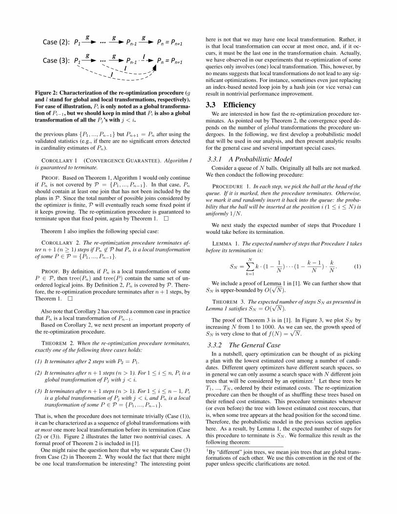
P1 Pn = Pn+1

g...

gPn-1

g

P1 Pn = Pn+1

g...

gPn-1

l

ll

Case (2):

Case (3):

Figure 2: Characterization of the re-optimization procedure (gand l stand for global and local transformations, respectively).For ease of illustration, Pi is only noted as a global transforma-tion of Pi−1, but we should keep in mind that Pi is also a globaltransformation of all the Pj’s with j < i.

the previous plans {P1, ..., Pn−1} but Pn+1 = Pn after using thevalidated statistics (e.g., if there are no significant errors detectedin cardinality estimates of Pn).

COROLLARY 1 (CONVERGENCE GUARANTEE). Algorithm 1is guaranteed to terminate.

PROOF. Based on Theorem 1, Algorithm 1 would only continueif Pn is not covered by P = {P1, ..., Pn−1}. In that case, Pn

should contain at least one join that has not been included by theplans in P . Since the total number of possible joins considered bythe optimizer is finite, P will eventually reach some fixed point ifit keeps growing. The re-optimization procedure is guaranteed toterminate upon that fixed point, again by Theorem 1.

Theorem 1 also implies the following special case:

COROLLARY 2. The re-optimization procedure terminates af-ter n+ 1 (n ≥ 1) steps if Pn 6∈ P but Pn is a local transformationof some P ∈ P = {P1, ..., Pn−1}.

PROOF. By definition, if Pn is a local transformation of someP ∈ P , then tree(Pn) and tree(P ) contain the same set of un-ordered logical joins. By Definition 2, Pn is covered by P . There-fore, the re-optimization procedure terminates after n+ 1 steps, byTheorem 1.

Also note that Corollary 2 has covered a common case in practicethat Pn is a local transformation of Pn−1.

Based on Corollary 2, we next present an important property ofthe re-optimization procedure.

THEOREM 2. When the re-optimization procedure terminates,exactly one of the following three cases holds:

(1) It terminates after 2 steps with P2 = P1.

(2) It terminates after n+ 1 steps (n > 1). For 1 ≤ i ≤ n, Pi is aglobal transformation of Pj with j < i.

(3) It terminates after n+ 1 steps (n > 1). For 1 ≤ i ≤ n− 1, Pi

is a global transformation of Pj with j < i, and Pn is a localtransformation of some P ∈ P = {P1, ..., Pn−1}.

That is, when the procedure does not terminate trivially (Case (1)),it can be characterized as a sequence of global transformations withat most one more local transformation before its termination (Case(2) or (3)). Figure 2 illustrates the latter two nontrivial cases. Aformal proof of Theorem 2 is included in [1].

One might raise the question here that why we separate Case (3)from Case (2) in Theorem 2. Why would the fact that there mightbe one local transformation be interesting? The interesting point

here is not that we may have one local transformation. Rather, itis that local transformation can occur at most once, and, if it oc-curs, it must be the last one in the transformation chain. Actually,we have observed in our experiments that re-optimization of somequeries only involves (one) local transformation. This, however, byno means suggests that local transformations do not lead to any sig-nificant optimizations. For instance, sometimes even just replacingan index-based nested loop join by a hash join (or vice versa) canresult in nontrivial performance improvement.

3.3 EfficiencyWe are interested in how fast the re-optimization procedure ter-

minates. As pointed out by Theorem 2, the convergence speed de-pends on the number of global transformations the procedure un-dergoes. In the following, we first develop a probabilistic modelthat will be used in our analysis, and then present analytic resultsfor the general case and several important special cases.

3.3.1 A Probabilistic ModelConsider a queue ofN balls. Originally all balls are not marked.

We then conduct the following procedure:

PROCEDURE 1. In each step, we pick the ball at the head of thequeue. If it is marked, then the procedure terminates. Otherwise,we mark it and randomly insert it back into the queue: the proba-bility that the ball will be inserted at the position i (1 ≤ i ≤ N ) isuniformly 1/N .

We next study the expected number of steps that Procedure 1would take before its termination.

LEMMA 1. The expected number of steps that Procedure 1 takesbefore its termination is:

SN =

N∑k=1

k · (1− 1

N) · · · (1− k − 1

N) · kN. (1)

We include a proof of Lemma 1 in [1]. We can further show thatSN is upper-bounded by O(

√N).

THEOREM 3. The expected number of steps SN as presented inLemma 1 satisfies SN = O(

√N).

The proof of Theorem 3 is in [1]. In Figure 3, we plot SN byincreasing N from 1 to 1000. As we can see, the growth speed ofSN is very close to that of f(N) =

√N .

3.3.2 The General CaseIn a nutshell, query optimization can be thought of as picking

a plan with the lowest estimated cost among a number of candi-dates. Different query optimizers have different search spaces, soin general we can only assume a search space with N different jointrees that will be considered by an optimizer.1 Let these trees beT1, ..., TN , ordered by their estimated costs. The re-optimizationprocedure can then be thought of as shuffling these trees based ontheir refined cost estimates. This procedure terminates whenever(or even before) the tree with lowest estimated cost reoccurs, thatis, when some tree appears at the head position for the second time.Therefore, the probabilistic model in the previous section applieshere. As a result, by Lemma 1, the expected number of steps forthis procedure to terminate is SN . We formalize this result as thefollowing theorem:1By “different” join trees, we mean join trees that are global trans-formations of each other. We use this convention in the rest of thepaper unless specific clarifications are noted.

0

10

20

30

40

50

60

70

0 100 200 300 400 500 600 700 800 900 1000

SN

N

(N, SN)

f(N)=√ N

g(N)=2√ N

Figure 3: SN with respect to the growth of N .

THEOREM 4. Assume that the position of a plan (after sampling-based validation) in the ordered plans with respect to their costs isuniformly distributed. Let N be the number of different join treesin the search space. 2 The expected number of steps before the re-optimization procedure terminates is then SN , where SN is com-puted by Equation 1. Moreover, SN = O(

√N) by Theorem 3.

We emphasize that the analysis here only targets worst-case per-formance, which might be too pessimistic. This is because Proce-dure 1 only simulates the Case (3) stated in Theorem 2, which isthe worst one among the three possible cases. In our experiments,we have found that all queries we tested require less than 10 roundsof iteration, most of which require only 1 or 2 rounds.

Remark: The uniformity assumption in Theorem 4 may not bevalid in practice. It is possible that a plan after sampling-based val-idation (or, a marked ball in terms of Procedure 1) is more likely tobe inserted into the front/back half of the queue. Such cases implythat, rather than with an equal chance of overestimation or under-estimation, the optimizer tends to overestimate/underestimate thecosts of all query plans (for a particular query). This is, however,not impossible. In practice, significant cardinality estimation er-rors usually appear locally and propagate upwards. Once the errorat some join is corrected, the errors in all plans that contain that joinwill also be corrected. In other words, the correction of the error ata single join can lead to the correction of errors in many candidateplans. In Appendix B, we further present analysis for two extremecases: all local errors are overestimates/underestimates. To sum-marize, for left-deep join trees, we have the following two results:

• If all local errors are overestimates, then in the worst case there-optimization procedure will terminate in at most m + 1steps, wherem is the number of joins contained in the query.

2Theoretically N could be as large as O(2m) where m is the num-ber of join operands, assuming that the optimizer uses the bottom-up dynamic programming search strategy. Nonetheless, this maynot always be the case. For example, some optimizers use the Cas-cades framework that leverages a top-down search strategy [18].An optimizer may even use different search strategies for differ-ent types of queries. For example, PostgreSQL will switch fromthe dynamic programming search strategy to a randomized searchstrategy based on genetic algorithm, when the number of joins ex-ceeds a certain threshold (12 by default) [2]. For this reason, wechoose to characterize the complexity of our algorithm in terms ofN rather than m.

• If all local errors are underestimates, then in the worst casere-optimization is expected to terminate in SN/M steps. HereN is the number of different join trees in the optimizer’ssearch space andM is the number of edges in the join graph.

Note that both results are better than the bound stated in Theorem 4.For instance, in the underestimation-only case, if N = 1000 andM = 10, we have SN = 39 but SN/M = 12.

However, in reality, overestimates and underestimates may co-exist. For left-deep join trees, by following the analysis in Ap-pendix B, we can see that such cases sit in between the two ex-treme cases. Nonetheless, an analysis for plans beyond left-deeptrees (e.g., bushy trees) seems to be challenging. We leave this asone possible direction for future work.

3.4 Optimality of the Final PlanWe can think of the re-optimization procedure as progressive ad-

justments of the optimizer’s direction when it explores its searchspace. The search space depends on the algorithm or strategy usedby the optimizer. So does the impact of re-optimization. But wecan still have some general conclusions about the optimality of thefinal plan regardless of the search space.

ASSUMPTION 1. The cost estimates of plans using sampling-based cardinality refinement are consistent. That is, for any twoplans P1 and P2, if costs(P1) < costs(P2), then costa(P1) <costa(P2). Here, costs(P ) and costa(P ) are the estimated costbased on sampling and the actual cost of plan P , respectively.

We have the following theorem based on Assumption 1. Theproof is included in [1].

THEOREM 5. Let P1, ..., Pn be a series of plans generated dur-ing the re-optimization procedure. Then costs(Pn) ≤ costs(Pi),and thus, by Assumption 1, it follows that costa(Pn) ≤ costa(Pi),for 1 ≤ i ≤ n− 1.

That is, the plan after re-optimization is guaranteed to be betterthan the original plan. Nonetheless, it is difficult to conclude thatthe plans are improved monotonically, namely, in general it is nottrue that costs(Pi+1) ≤ costs(Pi), for 1 ≤ i ≤ n − 1. However,we can prove that this is true if we only have overestimates duringre-optimization (proof in [1]):

COROLLARY 3. Let P1, ..., Pn be a series of plans generatedduring the re-optimization procedure. If in the re-optimization pro-cedure only overestimates occur, then costs(Pi+1) ≤ costs(Pi)for 1 ≤ i ≤ n− 1.

Our last result on the optimality of the final plan is in the sensethat it is the best among all the plans that are local transformationsof the final plan (proof in [1]).

THEOREM 6. Let P be the final plan the re-optimization pro-cedure returns. For any P ′ such that P ′ is a local transformationof P , it holds that costs(P ) ≤ costs(P ′).

3.5 DiscussionWe call the final plan returned by the re-optimization procedure

the fixed point with respect to the initial plan generated by the op-timizer. According to Theorem 5, this plan is a local optimum withrespect to the initial plan. Note that, if P = {P1, ..., Pn} coversthe whole search space, that is, any plan P in the search space iscovered by P , then the locally optimal plan is also globally opti-mal. However, in general, it is difficult to give a definitive answer

to the question that how far away the plan after re-optimization isfrom the true optimal plan. It depends on several factors, includingthe quality of the initial query plan, the search space covered byre-optimization, and the accuracy of the cost model and sampling-based cardinality estimates.

A natural question is then the impact of the initial plan. Intu-itively, it seems that the initial plan can affect both the fixed pointand the time it takes to converge to the fixed point. (Note that itis straightforward to prove that the fixed point must exist and beunique, with respect to the given initial plan.) There are also otherrelated interesting questions. For example, if we start with two ini-tial plans with similar cost estimates, would they converge to fixedpoints with similar costs as well? We leave all these problems asinteresting directions for further investigation.

Moreover, the convergence of the re-optimization procedure to-wards a fixed point can also be viewed as a validation procedure ofthe costs of the plans V that can be covered by P = {P1, ..., Pn}.Note that V is a subset of the whole search space explored by theoptimizer, and V is induced by P1 — the initial plan that is deemedas optimal by the optimizer. It is also interesting future work tostudy the relationship between P1 and V , especially how much ofthe complete search space can be covered by V .

4. OPTIMIZER “TORTURE TEST”Evaluating the effectiveness of a query optimizer is challenging.

As we mentioned in the introduction, query optimizers have to han-dle not only common cases but also difficult, corner cases. How-ever, we found it impossible to find well-known public examples ofthese corner-case queries and the data sets they run on. Regardingthis, in this section we create our own data sets and queries basedon the well-known fact that many difficult queries are made diffi-cult by correlation in the data [28]. We call it “optimizer torturetest” (OTT), given that our goal is to sufficiently challenge the car-dinality estimation approaches used by current query optimizers.We next describe the details of OTT.

4.1 Design of the Database and QueriesSince we target cardinality/selectivity estimation, we can focus

on queries that only contain selections and joins. In general, aselection-join query q over K relations R1, ..., RK can be rep-resented as

q = σF (R1 ./ · · · ./ RK),

where F is a selection predicate as in relational algebra (i.e., aboolean formula). Moreover, we can just focus on equality predi-cates, i.e., predicates of the formA = c whereA is an attribute andc is a constant. Any other predicate can be represented by unionsof equality predicates. As a result, we can focus on F of the form

F = (A1 = c1) ∧ · · · ∧ (AK = cK),

where Ak is an attribute of Rk, and ck ∈ Dom(Ak) (1 ≤ k ≤ K).Here, Dom(Ak) is the domain of the attribute Ak.

Based on the above observations, our design of the database andqueries is as follows:

(1) We have K relations R1(A1, B1), ..., RK(AK , BK).

(2) We use Ak’s for selections and Bk’s for joins.

(3) Let R′k = σAk=ck (Rk) for 1 ≤ k ≤ K. The queries of ourbenchmark are then of the form:

R′1 ./B1=B2 R′2 ./B2=B3 · · · ./BK−1=BK R′K . (2)

The remaining question is how to generate data forR1, ...,RK sothat we can easily control the selectivities for the selection and joinpredicates. This requires us to consider the joint data distributionfor (A1, ..., AK , B1, ..., BK). A straightforward way could be tospecify the contingency table of the distribution. However, thereis a subtle issue of this approach: we cannot just generate a largetable with attributes A1, ..., AK , B1, ..., BK and then split it intodifferent relations R1(A1, B1), ..., RK(AK , BK). The reason isthat we cannot infer the joint distribution (A1, ..., AK , B1, ..., BK)based on the (marginal) distributions we observed on (A1, B1), ...,(AK , BK). In Appendix C we further provide a concrete exampleto illustrate this. This discrepancy between the observed and truedistributions calls for a new approach.

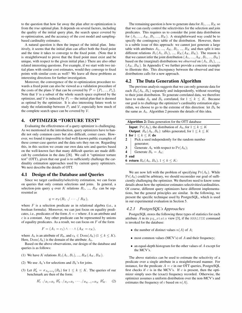
4.2 The Data Generation AlgorithmThe previous analysis suggests that we can only generate data for

each Rk(Ak, Bk) separately and independently, without resortingto their joint distribution. To generate correlated data, we thereforehave to make Ak and Bk correlated, for 1 ≤ k ≤ K. Becauseour goal is to challenge the optimizer’s cardinality estimation algo-rithm, we choose to go to the extreme of this direction: let Bk bethe same as Ak. Algorithm 2 presents the details of this idea.

Algorithm 2: Data generation for the OTT databaseInput: Pr(Ak), the distribution of Ak, for 1 ≤ k ≤ KOutput: Rk(Ak, Bk): tables generated, for 1 ≤ k ≤ K

1 for 1 ≤ k ≤ K do2 Pick a seed independently for the random number

generator;3 Generate Ak with respect to Pr(Ak);4 Generate Bk = Ak;5 end6 return Rk(Ak, Bk), 1 ≤ k ≤ K;

We are now left with the problem of specifying Pr(Ak). WhilePr(Ak) could be arbitrary, we should reconsider our goal of suffi-ciently challenging the optimizer. We therefore need to know somedetails about how the optimizer estimates selectivities/cardinalities.Of course, different query optimizers have different implementa-tions, but the general principles are similar. In the following, wepresent the specific technique used by PostgreSQL, which is usedin our experimental evaluation in Section 5.

4.2.1 PostgreSQL’s ApproachesPostgreSQL stores the following three types of statistics for each

attribute A in its pg_stats view [3], if the ANALYZE commandis invoked for the database:

• the number of distinct values n(A) of A;

• most common values (MCV’s) of A and their frequency;

• an equal-depth histogram for the other values ofA except forthe MCV’s.

The above statistics can be used to estimate the selectivity of apredicate over a single attribute in a straightforward manner. Forinstance, for the predicate A = c in our OTT queries, PostgreSQLfirst checks if c is in the MCV’s. If c is present, then the opti-mizer simply uses the (exact) frequency recorded. Otherwise, theoptimizer assumes a uniform distribution over the non-MCV’s andestimates the frequency of c based on n(A).

The approach used by PostgreSQL to estimate selectivities forjoin predicates is more sophisticated. Consider an equal-join predi-cateB1 = B2. If MCV’s for eitherB1 orB2 are not available, thenthe optimizer uses an approach first introduced in System R [35] byestimating the reduction factor as 1/max{n(B1), n(B2)}. If, onthe other hand, MCV’s are available for bothB1 andB2, then Post-greSQL tries to refine its estimate by first “joining” the two lists ofMCV’s. For skewed data distributions, this can lead to much betterestimates because the join size of the MCV’s, which is accurate,will be very close to the actual join size. Other database systems,such as Oracle [7], use similar approaches.

To combine selectivities from multiple predicates, PostgreSQLrelies on the well-known attribute-value-independence (AVI) as-sumption, which assumes that the distributions of values of dif-ferent attributes are independent.

4.2.2 The Distribution Pr(Ak) And Its ImpactFrom the previous discussion we can see that whether Pr(Ak) is

uniform or skewed will have little difference in affecting the opti-mizer’s estimates if MCV’s are leveraged, simply because MCV’shave recorded the exact frequency for those skewed values. Wetherefore can just let Pr(Ak) be uniform. We next analyze theimpact of this decision by computing the differences between theestimated and actual cardinalities for the OTT queries.

Let us first revisit the OTT queries presented in Equation 2. Notethat for an OTT query to be non-empty, the following conditionmust hold: B1 = B2 = · · · = BK−1 = BK . Because we haveintentionally set Ak = Bk for 1 ≤ k ≤ K, this then implies

A1 = A2 = · · · = AK−1 = AK . (3)

The query size can thus be controlled by the values of the A’s. Thequery is simply empty if Equation 3 does not hold. In Appendix D,we further present a detailed analysis of the query size when Equa-tion 3 holds. To summarize, we are able to control the differencebetween the query sizes when Equation 3 holds or not. Therefore,we can make this gap as large as we wish. However, the optimizerwill give the same estimate of the query size regardless of if Equa-tion 3 holds or not. In our experiments (Section 5) we further usedthis property to generate instance OTT queries.

5. EXPERIMENTAL EVALUATIONWe present experimental evaluation results of our proposed re-

optimization procedure in this section.

5.1 Experimental SettingsWe implemented the re-optimization framework in PostgreSQL

9.0.4. The modification to the optimizer is small, limited to sev-eral hundred lines of C code, which demonstrates the feasibility ofincluding our framework into current query optimizers. We con-ducted our experiments on a PC with 2.4GHz Intel dual-core CPUand 4GB memory, and we ran PostgreSQL under Linux 2.6.18.

5.1.1 Databases and Performance MetricsWe used both the standard version and a skewed version [4] of

the TPC-H benchmark database, as well as our own OTT databasedescribed in Section 4.

TPC-H Benchmark Databases. We used TPC-H databasesat the scale of 10GB in our experiments. The generator for skewedTPC-H database uses a parameter z to control the skewness ofeach column by generating Zipfian distributions. The larger z is,the more skewed the generated data are. z = 0 corresponds to a

uniform distribution. In our experiments, we generated a skeweddatabase by setting z = 1.

OTT Database. We created an instance of the OTT databasein the following manner. We first generated a standard 1GB TPC-H database. We then extended the 6 largest tables (lineitem, or-ders, partsupp, part, customer, supplier) by adding two additionalcolumns A and B to each of them. As discussed in Section 4.2,we populated the extra columns with uniform data. The domainof a column is determined by the number of rows in the corre-sponding table: if the table contains r rows, then the domain is{0, 1, ..., r/100 − 1}. In other words, each distinct value in thedomain appears roughly 100 times in the generated column. Wefurther created an index on each added column.

Performance Metrics. In our experiments, we measured thefollowing performance metrics for each query on each database:

(1) the original running time of the query;

(2) the number of iterations the re-optimization procedure requiresbefore its termination;

(3) the time spent on the re-optimization procedure;

(4) the total query running time including the re-optimization time.

Based on studies in the previous work [40], in all of our experi-ments we set the sampling ratio to be 0.05, namely, 5% of the datawere taken as samples.

5.1.2 Calibrating Cost ModelsThe previous work [40] has also shown that, after proper calibra-

tion of the cost models used by the optimizer, we could have betterestimates of query running times. An interesting question is then:would calibration also improve query optimization?

In our experiments, we also investigated this problem. Specifi-cally, we ran the offline calibration procedure (details in [40]) andreplaced the default values of the five cost units (seq_page_cost,random_page_cost, cpu_tuple_cost, cpu_index_tuple_cost, andcpu_operator_cost) in postgresql.conf (i.e., the configura-tion file of PostgreSQL server) with the calibrated values. In thefollowing, we also report results based on calibrated cost models.

5.2 Results on the TPC-H BenchmarkWe tested 21 TPC-H queries. (We excluded Q15, which is not

supported by our current implementation because it requires to cre-ate a view first.) For each TPC-H query, we randomly generated10 instances. We cleared both the database buffer pool and the filesystem cache between each run of each query.

5.2.1 Results on Uniform DatabaseFigure 4 presents the average running times and their standard

deviations (as error bars) of these queries over the uniform database.We have two observations. First, while the running times for

most of the queries almost do not change, we can see significant im-provement for some queries. For example, as shown in Figure 4(a),even without calibration of the cost units, the average running timeof Q9 drops from 4,446 seconds to only 932 seconds, a 79% re-duction; more significantly, the average running time of Q21 dropsfrom 20,746 seconds (i.e., almost 6 hours) to 3,508 seconds (i.e.,less than 1 hour), a 83% reduction.

Second, calibration of the cost units can sometimes significantlyreduce the running times for some queries. For example, compar-ing Figure 4(a) with Figure 4(b) we can observe that the average

0

2000

4000

6000

8000

10000

1 2 3 4 5 6 7 8 9 10 11 12 13 14 16 17 18 19 20 21 22

Run

ning

Tim

e (s

)

TPC-H Query

Original PlanRe-optimized Plan

(a) Without calibration of the cost units

0

2000

4000

6000

8000

10000

1 2 3 4 5 6 7 8 9 10 11 12 13 14 16 17 18 19 20 21 22

Run

ning

Tim

e (s

)

TPC-H Query


(b) With calibration of the cost units

Figure 4: Query running time over uniform 10GB TPC-Hdatabase (z = 0).

0

1

2

3

4

5

6

1 2 3 4 5 6 7 8 9 10 11 12 13 14 16 17 18 19 20 21 22

Num

ber

of P

lans

TPC-H Query

Without CalibrationWith Calibration

Figure 5: The number of plans generated during re-optimization over uniform 10GB TPC-H database.

running time of Q8 drops from 3,048 seconds to only 339 seconds,a 89% reduction, by just using calibrated cost units without eveninvoking the re-optimization procedure.

We further studied the re-optimization procedure itself. Figure 5presents the number of plans generated during re-optimization. Itsubstantiates our observation in Figure 4: for the queries whoserunning times were not improved, the re-optimization procedureindeed picked the same plans as those originally chosen by theoptimizer. Figure 6 further compares the query running time ex-cluding/including the time spent on re-optimization. For all thequeries we tested, re-optimization time is ignorable compared toquery execution time, which demonstrates the low overhead of ourre-optimization procedure.

5.2.2 Results on Skewed DatabaseOn the skewed database, we have observed results similar to that

on the uniform database. Figure 7 presents the running times ofthe queries, with or without calibration of the cost units.3 While itlooks quite similar to Figure 4, there is one interesting phenomenon3We notice that Q17 in Figure 7 has a large error bar. The errorbars represent variance due to different instances of the query tem-plate (different constants in the query). Q17 therefore has a largevariance, because we used a skewed TPC-H database. The varianceis much smaller when a uniform database is used (see Figure 4).

0

2000

4000

6000

8000

10000

1 2 3 4 5 6 7 8 9 10 11 12 13 14 16 17 18 19 20 21 22

Run

ning

Tim

e (s

)

TPC-H Query

Execution OnlyRe-optimization + Execution


0

2000

4000

6000

8000

10000

1 2 3 4 5 6 7 8 9 10 11 12 13 14 16 17 18 19 20 21 22

Run

ning

Tim

e (s

)

TPC-H Query



Figure 6: Query running time excluding/including re-optimization time over uniform 10GB TPC-H database (z = 0).

not shown before. In Figure 7(a) we see that, without using cali-brated cost units, the average running times for Q8 and Q9 actu-ally increase after re-optimization. Recall that in Section 3.4 wehave shown the local optimality of the plan returned by the re-optimization procedure (Theorem 5). However, that result is basedon the assumption that sampling-based cost estimates are consis-tent with actual costs (Assumption 1). Here this seems not thecase. Nonetheless, after using calibrated cost units, both the run-ning times of Q8 and Q9 were significantly improved (Figure 7(b)).

We further present the number of plans considered during re-optimization in Figure 8. Note that re-optimization seems to bemore active on skewed data. Figure 9 shows the running times ex-cluding/including the re-optimization times of the queries. Again,the additional overhead of re-optimization is trivial.

5.2.3 DiscussionWhile one might expect the chance for re-optimization to gen-

erate a better plan is higher on skewed databases, our experimentsshow that this may not be the case, at least for TPC-H queries.There are several different situations, though. First, if a query istoo simple, then there is almost no chance for re-optimization. Forexample, Q1 contains no join, whereas Q16 and Q19 involve onlyone join so only local transformations are possible. Second, the fi-nal plan returned by the re-optimization procedure heavily relies onthe initial plan picked by the optimizer, which is the seed or startingpoint where re-optimization originates. Note that, even if the opti-mizer has picked an inefficient plan, re-optimization cannot help ifthe estimated cost of that plan is not significantly erroneous. Onequestion is if this is possible: the optimizer picks an inferior planwhose cost estimate is correct? This actually could happen becausethe optimizer may (incorrectly) overestimate the costs of the otherplans in its search space. Another subtle point is that the inferiorplan might be robust to certain degree of errors in cardinality es-timates. Previous work has reported this phenomenon by noticingthat the plan diagram (i.e., all possible plans and their governed op-timality areas in the selectivity space) is dominated by just a coupleof query plans [33].

0

1000

2000

3000

4000

5000

6000

1 2 3 4 5 6 7 8 9 10 11 12 13 14 16 17 18 19 20 21 22

Run

ning

Tim

e (s

)

TPC-H Query



0

1000

2000

3000

4000

5000

6000

1 2 3 4 5 6 7 8 9 10 11 12 13 14 16 17 18 19 20 21 22

Run

ning

Tim

e (s

)

TPC-H Query



Figure 7: Query running time over skewed 10GB TPC-Hdatabase (z = 1).

0

1

2

3

4

5

6

1 2 3 4 5 6 7 8 9 10 11 12 13 14 16 17 18 19 20 21 22

Num

ber

of P

lans

TPC-H Query


Figure 8: The number of plans generated during re-optimization over skewed 10GB TPC-H database.

In summary, the effectiveness of re-optimization depends on fac-tors that are out of the control of the re-optimization procedure it-self. Nevertheless, we have observed intriguing improvement forsome long-running queries by applying re-optimization, especiallyafter calibration of the cost units.

5.3 Results of the Optimizer Torture TestWe created queries following our design of the OTT in Sec-

tion 4.1. Specifically, if a query contains n tables (i.e., n−1 joins),we letm of the selections beA = 0 (A = 1), and let the remainingn − m selections be A = 1 (A = 0). We generated two sets ofqueries: (1) n = 5 (4 joins), m = 4; and (2) n = 6 (5 joins),m = 4. Note that the maximal non-empty sub-queries then con-tain 3 joins over 4 tables with result size of roughly 1004 = 108

rows.4 However, the size of each (whole) query is 0. So we wouldlike to see the ability of the optimizer as well as the re-optimizationprocedure to identify the empty/non-empty sub-queries.

Figure 10 and 11 present the running times of the 4-join and 5-join queries, respectively. We generated in total 10 4-join queriesand 30 5-join queries. Note that the y-axes are in log scale and wedo not show queries that finish in less than 0.1 second. As we can4Recall that a non-empty query must have equal A’s (Equation 3)and we generated data with roughly 100 rows per distinct value(Section 5.1).

0

1000

2000

3000

4000

5000

6000

1 2 3 4 5 6 7 8 9 10 11 12 13 14 16 17 18 19 20 21 22

Run

ning

Tim

e (s

)

TPC-H Query



0

1000

2000

3000

4000

5000

6000

1 2 3 4 5 6 7 8 9 10 11 12 13 14 16 17 18 19 20 21 22

Run

ning

Tim

e (s

)

TPC-H Query



Figure 9: Query running time excluding/including re-optimization time over skewed 10GB TPC-H database (z = 1).

see, sometimes the optimizer failed to detect the existence of emptysub-queries: it generated plans where empty join predicates wereevaluated after the non-empty ones. The running times of thesequeries were then hundreds or even thousands of seconds. On theother hand, the re-optimization procedure did an almost perfect jobin detecting empty joins, which led to very efficient query planswhere the empty joins were evaluated first: all the queries afterre-optimization finished in less than 1 second.

We also did similar studies regarding the number of plans gener-ated during re-optimization and the time it consumed. Due to spaceconstraints, we refer the readers to Appendix A.1 for the details.

One might argue that the OTT queries are really contrived: thesequeries are hardly to see in real-world workloads. While this mightbe true, we think these queries serve our purpose as exemplify-ing extremely hard cases for query optimization. Note that hardcases are not merely long-running queries: queries as simple as se-quentially scanning huge tables are long-running too, but there isnothing query optimization can help with. Hard cases are querieswhere efficient execution plans do exist but it might be difficultfor the optimizer to find them. The OTT queries are just theseinstances. Based on the experimental results of the OTT queries,re-optimization is helpful to give the optimizer second chances if itinitially made a bad decision.

Another concern is if commercial database systems could do abetter job on the OTT queries. In regard of this, we also ran the OTTover two major commercial database systems. The performance isvery similar to that of PostgreSQL (Figure 12 and 13). We thereforespeculate that commercial systems could also benefit from our re-optimization technique proposed in this paper.

5.3.1 A Note on Multidimensional HistogramsNote that even using multidimensional histograms (e.g., [10, 31,

32]) may not be able to detect the data correlation presented in theOTT queries, unless the buckets are so fine-grained that the exactjoint distributions are retained. To understand this, let us considerthe following example.

0.1

1

10

100

1000

10000

1 2 3 4 5 6 7 8 9 10

Run

ning

Tim

e (s

)

OTT Query

Original Plan Re-optimized Plan


0.1

1

10

100

1000

10000

1 2 3 4 5 6 7 8 9 10

Run

ning

Tim

e (s

)

OTT Query



Figure 10: Query running times of 4-join queries.

0.1

1

10

100

1000

10000

1 2 3 4 5 6 7 8 9 10 11 12 13 14 15 16 17 18 19 20 21 22 23 24 25 26 27 28 29 30

Run

ning

Tim

e (s

)

OTT Query



0.1

1

10

100

1000

10000

1 2 3 4 5 6 7 8 9 10 11 12 13 14 15 16 17 18 19 20 21 22 23 24 25 26 27 28 29 30

Run

ning

Tim

e (s

)

OTT Query



Figure 11: Query running times of 5-join queries.

EXAMPLE 2. Following our design of OTT, suppose that nowwe only have two tables R1(A1, B1) and R2(A2, B2). Moreover,suppose that each Ak (and thus Bk) contains m = 2l distinctvalues, and we construct (perfect) 2-dimensional histograms on(Ak, Bk) (k = 1, 2). Each dimension is evenly divided into m

2= l

intervals, so each histogram contains l2 buckets. The joint distri-bution over (Ak, Bk) estimated by using the histogram is then:{

Pr(2r − 2 ≤ Ak < 2r, 2r − 2 ≤ Bk < 2r) = 1l, 1 ≤ r ≤ l;

Pr(al ≤ Ak < a2, b1 ≤ Bk < b2) = 0, otherwise.

For instance, if m = 100, then l = 50. So we have Pr(0 ≤ Ak <2, 0 ≤ Bk < 2) = · · · = Pr(98 ≤ Ak < 100, 98 ≤ Bk <100) = 1

50, while all the other buckets are empty. On the other

0.1

1

10

100

1000

10000

1 2 3 4 5 6 7 8 9 10

Run

ning

Tim

e (s

)

OTT Query

Original Plan

(a) 4-join OTT queries

0.1

1

10

100

1000

10000

1 2 3 4 5 6 7 8 9 10 11 12 13 14 15 16 17 18 19 20 21 22 23 24 25 26 27 28 29 30

Run

ning

Tim

e (s

)

OTT Query

Original Plan

(b) 5-join OTT queries

Figure 12: Query running times of the OTT queries on the com-mercial database system A.

0.1

1

10

100

1000

10000

1 2 3 4 5 6 7 8 9 10

Run

ning

Tim

e (s

)

OTT Query

Original Plan

(a) 4-join OTT queries

0.1

1

10

100

1000

10000

1 2 3 4 5 6 7 8 9 10 11 12 13 14 15 16 17 18 19 20 21 22 23 24 25 26 27 28 29 30

Run

ning

Tim

e (s

)

OTT Query

Original Plan

(b) 5-join OTT queries

Figure 13: Query running times of the OTT queries on the com-mercial database system B.

hand, the actual joint distribution is

Pr(Ak = a,Bk = b) =

{1m, if a = b;

0, otherwise.

Now, let us consider the selectivities for two OTT queries:

(q1) σA1=0∧A2=1∧B1=B2(R1 ×R2);

(q2) σA1=0∧A2=0∧B1=B2(R2 ×R2).

We know that q1 is empty but q2 is not. However, the estimated se-lectivity (and thus cardinality) of q1 and q2 is the same by using the

100

1000

10000

1 2 3 4 5

Run

ning

Tim

e (s

)

Round

Q8Q9Q21

Figure 14: Running time of plans generated in re-optimizationfor TPC-H queries (z = 0) without calibration of cost units.

2-dimensional histogram, because of the assumption used by his-tograms that data inside each bucket is uniformly distributed.5 Withthe setting used in our experiments, m = 100 and thus l = 50. Soeach 2-dimensional histogram contains l2 = 2, 500 buckets. How-ever, even such detailed histograms cannot help the optimizer dis-tinguish empty joins from nonempty ones. Furthermore, note thatour conclusion is independent of m, while the number of bucketsincreases quadratically in m. For instance, when m = 104 whichmeans we have histograms containing 2.5× 107 buckets, the opti-mizer still cannot rely on the histograms to generate efficient queryplans for OTT queries.

5.4 Effectiveness of IterationOne interesting further question is how much benefit iteration

brings in. Since running plans over samples incurs additional cost,we may wish to stop the iteration as early as possible rather thanwait until its convergence. To investigate this, we also tested ex-ecution times for plans generated during re-optimization on theoriginal databases. We focus on queries for which at least twoplans were generated. Figure 14 presents typical results for TPC-Hqueries Q8, Q9, and Q21, and Figure 15 presents typical results forthe OTT queries. For each query, the plan in the first round is theoriginal one returned by the optimizer.

We have the following observations. While the plan returned inthe second round of iteration (i.e., the first different plan returnedby re-optimization) often dramatically reduces the query executiontime, it is not always the case. Sometimes it takes additional roundsbefore an improved plan is found while the plans generated in be-tween have similar execution times (e.g., 4-join OTT query Q8 and5-join OTT query Q13). In the case of TPC-H Q21, the executiontimes of intermediate plans generated during re-optimization areeven not non-increasing. The plans returned by the optimizer in thesecond and third round are even much worse than the original plan.(Note that the y-axis of Figure 14 is in log scale.) Fortunately, bycontinuing with the iteration, we can eventually reach a plan that ismuch better than the original one.

The above observations give rise to the question why worse plansmight be generated during re-optimization. To understand this, notethat in the middle of re-optimization, the plans returned by the op-timizer are based on statistics that are partially validated by sam-pling. The optimizer is likely to generate an “optimal” plan dueto underestimating the costs of joins that have not been coveredby plans generated in previous rounds. This phenomenon has alsobeen observed in previous work [13]. It is the essential reason thatwe cannot make Theorem 5 stronger. As long as there exist un-covered joins, there is no guarantee on the plan returned by theoptimizer. Only upon the convergence of re-optimization we can

5It is easy to verify that the selectivity estimates are s1 = s2 = 18l2

.

0.0001 0.001 0.01 0.1

1 10

100 1000

10000

1 2 3 4

Run

ning

Tim

e (s

)

Round

Q5Q8Q9

(a) 4-join queries

0.0001 0.001 0.01 0.1

1 10

100 1000

10000

1 2 3 4

Run

ning

Tim

e (s

)

Round

Q7Q13Q14

(b) 5-join queries

Figure 15: Running time of plans generated in re-optimizationfor the OTT queries without calibration of cost units.

say that the final plan is locally optimal.Nevertheless, in practice we can still have various strategies to

control the overhead of re-optimization. For example, we can stopre-optimization if it does not converge after a certain number ofrounds, or if the time spent on re-optimization has reached sometimeout threshold. We then simply return the best plan among theplans generated so far, based on their cost estimates by using re-fined cardinality estimates from sampling [40]. As another option,it might even be worth considering not doing re-optimization at allif the estimated query execution time is shorter than some thresh-old, or only doing it if we run that plan and get past that thresholdwithout being close to done.

6. RELATED WORKQuery optimization has been studied for decades, and we refer

the readers to [12] and [22] for surveys in this area.Cardinality estimation is a critical problem in cost-based query

optimization, and has triggered extensive research in the databasecommunity. Approaches for cardinality estimation in the litera-ture are either static or dynamic. Static approaches usually relyon various statistics that are collected and maintained periodicallyin an off-line manner, such as histograms (e.g., [23, 32]), samples(e.g., [11, 20, 27]), sketches (e.g., [5, 34]), or even graphical mod-els (e.g. [17, 37]). In practice, approaches based on histogramsare dominant in the implementations of current query optimizers.However, histogram-based approaches have to rely on the notori-ous attribute-value-independence (AVI) assumption, and they oftenfail to capture data correlations, which could result in significanterrors in cardinality estimates. While variants of histograms (inparticular, multidimensional histograms, e.g., [10, 31, 32]) havebeen proposed to overcome the AVI assumption, they suffer fromsignificantly increased overhead on large databases. Meanwhile,even if we can afford the overhead of using multidimensional his-tograms, they are still insufficient in many cases, as we discussed inSection 5.3.1. Compared with histogram-based approaches, sam-pling is better at capturing data correlation. One reason for this

is that sampling evaluates queries on real rather than summarizeddata. There are many sampling algorithms, and in this paper we justpicked a simple one (see [38] for a recent survey). We do not try toexplore more advanced sampling techniques (e.g. [16]), which webelieve could further improve the quality of cardinality estimates.

On the other hand, dynamic approaches further utilize informa-tion gathered during query runtime. Approaches in this directioninclude dynamic query plans (e.g., [14, 19]), parametric query op-timization (e.g. [24]), query feedback (e.g., [8, 36]), mid-query re-optimization (e.g. [25, 30]), and quite recently, plan bouquets [15].The ideas behind dynamic query plans and parametric query opti-mization are similar: rather than picking one single optimal queryplan, all possible optimal plans are retained and the decision is de-ferred until runtime. Both approaches suffer from the problem ofcombinatorial explosion and are usually used in contexts where ex-pensive pre-compilation stages are affordable. The recent devel-opment of plan bouquets [15] is built on top of parametric queryoptimization so it may also incur a heavy query compilation stage.

Meanwhile, approaches based on query feedback record statis-tics of past queries and use this information to improve cardinalityestimates for future queries. Some of these approaches have beenadopted in commercial systems such as IBM DB2 [36] and Mi-crosoft SQL Server [8]. Nonetheless, collecting query feedbackincurs additional runtime overhead as well as storage overhead ofever-growing volume of statistics.

The most relevant work in the literature is the line along mid-query re-optimization [25, 30]. The major difference is that re-optimization was previously carried out at runtime over the actualdatabase rather than at query compilation time over the samples.The main issue is the trade-off between the overhead spent on re-optimization and the improvement on the query plan. In the intro-duction, we have articulated the pros and cons of both techniques.In some sense, our approach can be thought of as a “dry run” ofruntime re-optimization. But it is much cheaper because it is per-formed over the sampled data. As we have seen, cardinality esti-mation errors due to data correlation can be caught by the sampleruns. So it is perhaps an overkill to detect these errors at runtimeby running the query over the actual database. Sometimes opti-mizers make mistakes that involve a bad ordering that results ina larger than expected result from a join or a selection. It is truethat runtime re-optimization can detect this, but this may requirethe query evaluator to do a substantial amount of work before itis detected. For example, if the data is fed into an operator in anon-random order, because of an unlucky ordering the fact that theoperator has a much larger than expected result may not be obvi-ous until a substantial portion of the input has been consumed andsubstantial system resources have been expended. Furthermore, itis non-trivial to stop an operator in mid-flight and switch to a dif-ferent plan — for this reason most runtime query re-optimizationdeals with changing plans at pipeline boundaries. Running a badplan until a pipeline completes might be very expensive.

Nonetheless, we are not claiming that we should just use ourapproach. Rather, our approach is complementary to runtime re-optimization techniques: it is certainly possible to apply those tech-niques on the plan returned by our approach. The hope is that, afterapplying our approach, the chance that we need to invoke morecostly runtime re-optimizaton techniques can be significantly re-duced. This is similar to the “alerter” idea that has been used inphysical database tuning [9], where a lightweight “alerter” is in-voked to determine the potential performance gain before the morecostly database tuning advisor is called. There is also some recentwork on applying runtime re-optimization to Map-Reduce basedsystems [26]. The “pilot run” idea explored in this work is close

to our motivation, where the goal is also to avoid starting with abad plan by collecting more accurate statistics via scanning a smallamount of samples. However, currently “pilot run” only collectsstatistics for leaf tables. It is then interesting to see if “pilot run”could be further enhanced by considering our technique.

In some sense, our approach sits between existing static and dy-namic approaches. We combine the advantage of lower overheadsfrom static approaches and the advantage of more optimization op-portunities from dynamic approaches. This compromise leads toa lightweight query re-optimization procedure that could bring upbetter query plans. However, this also unavoidably leads to the co-existence of both histogram-based and sampling-based cardinalityestimates during re-optimization, which may cause inconsistencyissues [29]. Somehow, this is a general problem when differenttypes of cardinality estimation techniques are used together. Forexample, an optimizer that also uses multi-dimensional histograms(in addition to one-dimensional histograms) may also have to han-dle inconsistencies. Previous runtime re-optimization techniquesare also likely to suffer similar issues. In this sense, this is an or-thogonal problem and we do not try to address it in this paper. Inspite of that, it is interesting future work to see how much more im-provement we can get if we further incorporate the approach basedon the maximum entropy principle [29] into our re-optimizationframework to resolve inconsistency in cardinality estimates.

Finally, we note that we are not the first that investigates the ideaof incorporating sampling into query optimization. Ilyas et al. pro-posed using sampling to detect data correlations and then collectingjoint statistics for those correlated data columns [21]. However,this seems to be insufficient if data correlation is caused by spe-cific selection predicates, such as those OTT queries used in ourexperiments. Babcock and Chaudhuri also investigated the usageof sampling in developing a robust query optimizer [6]. While ro-bustness is another interesting goal for query optimizer, it is beyondthe scope of this paper.

7. CONCLUSIONIn this paper, we studied the problem of incorporating sampling-

based cardinality estimates into query optimization. We proposedan iterative query re-optimization procedure that supplements theoptimizer with refreshed cardinality estimates via sampling andgives it second chances to generate better query plans. We showthe efficiency and effectiveness of this re-optimization procedureboth theoretically and experimentally.

There are several directions worth further exploring. First, aswe have mentioned, the initial plan picked by the optimizer mayhave great impact on the final plan returned by re-optimization.While it remains interesting to study this impact theoretically, itmight also be an intriguing idea to think about varying the way thatthe query optimizer works. For example, rather than just return-ing one plan, the optimizer could return several candidates and letthe re-optimization procedure work on each of them. This mightmake up for the potentially bad situation currently faced by the re-optimization procedure that it may start with a bad seed plan. Sec-ond, the re-optimization procedure itself could be further improved.As an example, note that in this paper we let the optimizer un-conditionally accept cardinality estimates by sampling. However,sampling is by no means perfect. A more conservative approachis to consider the uncertainty of the cardinality estimates returnedby sampling as well. The previous work [41] has investigated theproblem of quantifying uncertainty in sampling-based query run-ning time estimation. It is very interesting to study a combinationof that framework with the re-optimization procedure proposed inthis paper. We leave all these as promising areas for future work.

Acknowledgements. We thank the anonymous reviewers for theirvaluable comments, and we thank Heng Guo for his help with theproof of Theorem 3. This work was supported in part by a GoogleFocus Award.

8. REFERENCES[1] http://arxiv.org/abs/1601.05748.[2] http://www.postgresql.org/docs/9.0/static/runtime-config-query.html.[3] http://www.postgresql.org/docs/9.0/static/view-pg-stats.html.[4] Skewed tpc-h data generator.

ftp://ftp.research.microsoft.com/users/viveknar/TPCDSkew/.[5] N. Alon, P. B. Gibbons, Y. Matias, and M. Szegedy. Tracking join

and self-join sizes in limited storage. In PODS, 1999.[6] B. Babcock and S. Chaudhuri. Towards a robust query optimizer: A

principled and practical approach. In SIGMOD, pages 119–130,2005.

[7] W. Breitling. Joins, skew and histograms.http://www.centrexcc.com/Joins,SkewandHistograms.pdf.

[8] N. Bruno and S. Chaudhuri. Exploiting statistics on queryexpressions for optimization. In SIGMOD, pages 263–274, 2002.

[9] N. Bruno and S. Chaudhuri. To tune or not to tune? A lightweightphysical design alerter. In VLDB, pages 499–510, 2006.

[10] N. Bruno, S. Chaudhuri, and L. Gravano. Stholes: Amultidimensional workload-aware histogram. In SIGMOD, pages211–222, 2001.

[11] M. Charikar, S. Chaudhuri, R. Motwani, and V. R. Narasayya.Towards estimation error guarantees for distinct values. In PODS,pages 268–279, 2000.

[12] S. Chaudhuri. An overview of query optimization in relationalsystems. In PODS, pages 34–43, 1998.

[13] S. Chaudhuri, V. R. Narasayya, and R. Ramamurthy. Apay-as-you-go framework for query execution feedback. PVLDB,1(1):1141–1152, 2008.

[14] R. L. Cole and G. Graefe. Optimization of dynamic query evaluationplans. In SIGMOD, pages 150–160, 1994.

[15] A. Dutt and J. R. Haritsa. Plan bouquets: query processing withoutselectivity estimation. In SIGMOD, 2014.

[16] C. Estan and J. F. Naughton. End-biased samples for join cardinalityestimation. In ICDE, 2006.

[17] L. Getoor, B. Taskar, and D. Koller. Selectivity estimation usingprobabilistic models. In SIGMOD, 2001.

[18] G. Graefe. The cascades framework for query optimization. IEEEData Eng. Bull., 18(3):19–29, 1995.

[19] G. Graefe and K. Ward. Dynamic query evaluation plans. InSIGMOD Conference, pages 358–366, 1989.

[20] P. J. Haas, J. F. Naughton, S. Seshadri, and A. N. Swami. Selectivityand cost estimation for joins based on random sampling. J. Comput.Syst. Sci., 52(3):550–569, 1996.

[21] I. F. Ilyas, V. Markl, P. J. Haas, P. Brown, and A. Aboulnaga.CORDS: automatic discovery of correlations and soft functionaldependencies. In SIGMOD, pages 647–658, 2004.

[22] Y. E. Ioannidis. Query optimization. ACM Comput. Surv.,28(1):121–123, 1996.

[23] Y. E. Ioannidis. The history of histograms (abridged). In VLDB,pages 19–30, 2003.

[24] Y. E. Ioannidis, R. T. Ng, K. Shim, and T. K. Sellis. Parametric queryoptimization. In VLDB, pages 103–114, 1992.

[25] N. Kabra and D. J. DeWitt. Efficient mid-query re-optimization ofsub-optimal query execution plans. In SIGMOD, pages 106–117,1998.

[26] K. Karanasos, A. Balmin, M. Kutsch, F. Ozcan, V. Ercegovac,C. Xia, and J. Jackson. Dynamically optimizing queries over largescale data platforms. In SIGMOD, pages 943–954, 2014.

[27] R. J. Lipton, J. F. Naughton, and D. A. Schneider. Practicalselectivity estimation through adaptive sampling. In SIGMOD, pages1–11, 1990.

[28] G. Lohman. Is query optimization a “solved” problem?http://wp.sigmod.org/?p=1075.

[29] V. Markl, P. J. Haas, M. Kutsch, N. Megiddo, U. Srivastava, and

T. M. Tran. Consistent selectivity estimation via maximum entropy.VLDB J., 16(1):55–76, 2007.

[30] V. Markl, V. Raman, D. E. Simmen, G. M. Lohman, and H. Pirahesh.Robust query processing through progressive optimization. InSIGMOD, pages 659–670, 2004.

[31] M. Muralikrishna and D. J. DeWitt. Equi-depth histograms forestimating selectivity factors for multi-dimensional queries. InSIGMOD, pages 28–36, 1988.

[32] V. Poosala and Y. E. Ioannidis. Selectivity estimation without theattribute value independence assumption. In VLDB, 1997.

[33] N. Reddy and J. R. Haritsa. Analyzing plan diagrams of databasequery optimizers. In VLDB, 2005.

[34] F. Rusu and A. Dobra. Sketches for size of join estimation. ACMTrans. Database Syst., 33(3), 2008.

[35] P. G. Selinger, M. M. Astrahan, D. D. Chamberlin, R. A. Lorie, andT. G. Price. Access path selection in a relational databasemanagement system. In SIGMOD, 1979.

[36] M. Stillger, G. M. Lohman, V. Markl, and M. Kandil. LEO - DB2’slearning optimizer. In VLDB, 2001.

[37] K. Tzoumas, A. Deshpande, and C. S. Jensen. Lightweight graphicalmodels for selectivity estimation without independence assumptions.PVLDB, 4(11):852–863, 2011.

[38] D. Vengerov, A. C. Menck, M. Zaït, and S. Chakkappen. Join sizeestimation subject to filter conditions. PVLDB, 8(12):1530–1541,2015.

[39] W. Wu, Y. Chi, H. Hacigümüs, and J. F. Naughton. Towardspredicting query execution time for concurrent and dynamic databaseworkloads. PVLDB, 6(10):925–936, 2013.

[40] W. Wu, Y. Chi, S. Zhu, J. Tatemura, H. Hacigümüs, and J. F.Naughton. Predicting query execution time: Are optimizer costmodels really unusable? In ICDE, pages 1081–1092, 2013.

[41] W. Wu, X. Wu, H. Hacigümüs, and J. F. Naughton. Uncertainty awarequery execution time prediction. PVLDB, 7(14):1857–1868, 2014.

APPENDIXA. ADDITIONAL RESULTS

In this section, we present additional experimental results for theOTT queries. We also performed the same experiments for TPC-DS queries, and we report the results here.

A.1 Additional Results on OTT QueriesFor OTT queries, we also did similar studies regarding the num-

ber of plans generated during re-optimization and the time it con-sumed. Figure 16 presents the number of plans generated dur-ing the re-optimization procedure for the 4-join and 5-join OTTqueries. Figure 17 and 18 further present the comparisons of therunning times by excluding or including re-optimization times forthese queries (the y-axes are in log scale).

A.2 Results on the TPC-DS BenchmarkWe conducted the same experiments on the TPC-DS benchmark.

Specifically, we use a subset containing 29 TPC-DS queries that aresupported by PostgreSQL and our current implementation, and weuse a 10GB TPC-DS database. The experiments were performedon a PC with 3.4GHz Intel 4-core CPU and 8GB memory, and weran PostgreSQL under Linux 2.6.32.

We again use a sampling ratio of 5%. Figure 19 presents theexecution time of each TPC-DS query. The time spent on runningquery plans over the samples is again trivial and therefore is notplotted. Figure 20 further presents the number of plans generatedduring re-optimization.6

6The results we show here are based on the TPC-DS database withonly indexes on primary keys of the tables. The TPC-DS bench-mark specification does not recommend any indexes, which poten-tially could have impact on the optimizer’s choices. Regarding this,

0 1 2 3 4 5 6 7 8

1 2 3 4 5 6 7 8 9 10

Num

ber

of P

lans

OTT Query

Without Calibration With Calibration

(a) 4-join queries

0

1

2

3

4

5

1 2 3 4 5 6 7 8 9 10 11 12 13 14 15 16 17 18 19 20 21 22 23 24 25 26 27 28 29 30

Num

ber

of P

lans

OTT Query

Without Calibration With Calibration

(b) 5-join queries

Figure 16: The number of plans generated during re-optimization for the OTT queries.

Unfortunately, we do not observe remarkable improvement overthe TPC-DS queries we tested by using re-optimization. Thereare several reasons. First, the majority of the queries are short-running ones, though some of them are quite complicated in termsof their query plans. There is little room for improvement on thesequeries. Second, for the four relatively long-running queries Q28,Q50, Q55, and Q65 (with running time above 100 seconds), threeof them (Q28, Q55, and Q65) are a bit trivial for re-optimization tohave impact. Q28 only accesses one table, while Q55 joins a facttable with two small dimension tables. Q65 involves joins betweena fact table and three small dimension tables, but its execution timeis dominated by a self-join over the fact table. Meanwhile, afterchecking the plans, we found that all cardinality estimates are ontrack. We therefore cannot observe a plan change for any of thesethree queries (see Figure 20). Third, even if there are significanterrors in cardinality estimates, they may not lead to significant im-provement on the query plan. This is the case for Q50, which in-volves joins over two fact tables and three dimension tables. Theexecution time is then dominated by the join between the two facttables. The optimizer’s cardinality estimate for that join is indeedinaccurate, and the error was successfully detected by using sam-pling. As a result, re-optimization did generate different accesspaths for the rest of the plan. However, the execution time of theplan remains to be dominated by that huge join, and the remainingexecution time after that dominant join was done is trivial.

We actually further tweaked Q50 by modifying the predicatesover the dimension tables so that the selectivity estimates werechanged. By doing this, we did identify cases where re-optimizationsignificantly reduced query execution times. We show one suchvariant of Q50 (i.e., Q50’) in Figure 19. The execution time ofQ50’ dropped from around 300 seconds to around 130 seconds af-ter re-optimization, a 57% reduction. Tweaking the other queriesmay also give more opportunities for re-optimization. Another way

we actually further tried to build indexes on columns that are ref-erenced by the queries. However, the results we obtained are verysimilar to the ones we present here.

0.0001

0.001

0.01

0.1

1

10

1 2 3 4 5 6 7 8 9 10

Run

ning

Tim

e (s

)

OTT Query

Executioin OnlyExecution + Re-optimized


0.001

0.01

0.1

1

10

1 2 3 4 5 6 7 8 9 10

Run

ning

Tim

e (s

)

OTT Query



Figure 17: Query running time excluding/including re-optimization time for the 4-join OTT queries.

0.0001

0.001

0.01

0.1

1

1 2 3 4 5 6 7 8 9 10 11 12 13 14 15 16 17 18 19 20 21 22 23 24 25 26 27 28 29 30

Run

ning

Tim

e (s

)

OTT Query



0.001

0.01

0.1

1

1 2 3 4 5 6 7 8 9 10 11 12 13 14 15 16 17 18 19 20 21 22 23 24 25 26 27 28 29 30

Run

ning

Tim

e (s

)

OTT Query



Figure 18: Query running time excluding/including re-optimization time for the 5-join OTT queries.

is to further change the distribution that governs the underlying datageneration. We do not pursue these options any further, for it re-mains debatable that these variants might just be contrived. A moresystematic way could be to identify a particular class of queries thatthe current optimizers do not handle well, figure out how to handlethese queries, then move on to find other kinds of queries that arestill not handled well. We suspect (and hope) that this is one wayoptimizers will improve over time — our work on creating the “op-timizer torture test” in Section 4 is one step in this direction. Weleave the study of other types of “difficult” queries as importantdirection for future work.

0

100

200

300

400

500

600

3 7 15 17 19 25 26 28 29 42 43 45 48 50 50’ 52 55 61 62 65 69 72 73 84 85 90 91 93 96 99

Run

ning

Tim

e (s

)

TPC-DS Query



0

100

200

300

400

500

600

3 7 15 17 19 25 26 28 29 42 43 45 48 50 50’ 52 55 61 62 65 69 72 73 84 85 90 91 93 96 99

Run

ning

Tim

e (s

)

TPC-DS Query



Figure 19: Query running time over 10GB TPC-DS database.

0

1

2

3

4

5

3 7 15 17 19 25 26 28 29 42 43 45 48 50 50’ 52 55 61 62 65 69 72 73 84 85 90 91 93 96 99

Num

ber

of P

lans

TPC-DS Query


Figure 20: The number of plans generated during re-optimization over 10GB TPC-DS database.

B. ADDITIONAL ANALYSISContinuing with our study of the efficiency of the re-optimization

procedure in Section 3.3, we now consider two special cases wherethe optimizer significantly overestimates or underestimates the se-lectivity of a particular join in the returned optimal plan. We focusour discussion on left-deep join trees. Before we proceed, we needthe following assumption of cost functions.

ASSUMPTION 2. Cost functions used by the optimizer are mono-tonically non-decreasing functions of input cardinalities.

We are not aware of a cost function that does not conform to thisassumption, though.

B.1 Overestimation OnlySuppose that the error is an overestimate, that is, the actual car-

dinality is smaller than the one estimated by the optimizer. Let thatjoin operator be O, and let the corresponding subtree rooted at Obe tree(O). Now consider a candidate plan P in the search space,and let cost(P ) be the estimated cost of P . Note that the followingproperty holds:

LEMMA 2. cost(P ) is affected (i.e., subject to change) only iftree(O) is a subtree of tree(P ).

Moreover, under Assumption 2, the refined cost estimate cost′(P )satisfies cost′(P ) < cost(P ) because of the overestimate. There-

Plans with tree(O)

as subtreeThe other plans

All plans

O

tree(O)

(a) Overestimation Only

Plans with tree(O)

as subtree

The other plans

(Plan P w/ min-cost)

O

tree(O)

(b) Underestimation Only

All plans

Figure 21: Comparison of the space of candidate optimalplans when local estimation errors are overestimation-only orunderestimation-only. Candidate optimal plans are shaded.

fore, if we let the set of all such plans P beP , then the next optimalplan picked by the optimizer must be from P . We thus can provethe following result:

THEOREM 7. Suppose that we only consider left-deep join trees.Let m be the number of joins in the query. If all estimation errorsare overestimates, then in the worst case the re-optimization proce-dure will terminate in at most m+ 1 steps.

The proof of Theorem 7 is included in [1]. We emphasize thatm+1 is a worst-case upper bound. The intuition behind Theorem 7is that, for left-deep join trees, the validated subtree belonging tothe final re-optimized plan can grow by at least one more level (i.e.,with one more validated join) in each re-optimization step.

B.2 Underestimation OnlySuppose that, on the other hand, the error is an underestimate,

that is, the actual cardinality is larger than the one estimated bythe optimizer. Then things become more complicated: not onlythose plans that contain the subtree rooted at the erroneous nodebut the plan with the lowest estimated cost in the rest of the searchspace (which is not affected by the estimation error) also has thepotential of being the optimal plan, after the error is corrected (seeFigure 21). We next again focus on left-deep trees and present someanalysis in such context.

Suppose that the join graph G contains M edges. We partitionthe join trees based on their first joins, which must be the edges ofG. So we have M partitions in total.

Let si be the state when a plan returned by the optimizer uses thei-th edge in G (1 ≤ i ≤ M ) as its first join. The re-optimizationprocedure can then be thought of as transitions between these Mstates, i.e., a Markov chain. Assume that the equilibrium state dis-tribution π(si) of this Markov chain exists, subject to∑M

i=1π(si) = 1.

π(si) therefore represents the probability that a plan generated inthe re-optimization procedure would have its first join in the parti-tion i (1 ≤ i ≤ M ). We can then estimate the expected number ofsteps before the procedure terminates as

S =∑M

i=1π(si) ·Ni,

whereNi is the number of steps/transitions confined in the partitioni before termination. Since we only consider left-deep trees, Ni =Nj for 1 ≤ i, j ≤ M . As a result, S can be simplified as S = Ni.So we are left with estimating Ni.Ni is the expected number of steps before termination if the tran-

sitions (i.e., re-optimization steps) are confined in the partition i.We can divide this process into stages, and each stage contains onemore join than the previous stage. If there are m joins, then wewill have m stages. In each stage, we go through every plan until

we finish, and the average number of plans we considered is SKj

as computed by Equation 1, where Kj is the number of join-trees(actually subtrees) in the stage j (1 ≤ j ≤ m). So

S = Ni =∑m

j=1SKj .

As an upper bound, we have S ≤ SN/M , whereN is the total num-ber of different join trees considered by the optimizer, and SN/M iscomputed by Equation 1. This is obtained by applying Theorem 4to each partition. SN/M is usually much smaller than SN , accord-ing to Figure 3. Again, we emphasize that the analysis here onlytargets worst-case expectations, which might be too pessimistic.

C. JOINT/MARGINAL DISTRIBUTIONSTo see why the straightforward approach that first generates a re-

lation (A1, ..., AK , B1, ..., BK) based on the joint distribution andthen splits it into different relation R1(A1, B1), ..., RK(AK , BK)is incorrect, let us consider the following example.

EXAMPLE 3. Suppose that we need to generate binary valuesfor two attributes A1 and A2, with the following joint distribution:

(1) p00 = Pr(A1 = 0, A2 = 0) = 0.1;

(2) p01 = Pr(A1 = 0, A2 = 1) = 0;

(3) p10 = Pr(A1 = 1, A2 = 0) = 0;

(4) p11 = Pr(A1 = 1, A2 = 1) = 0.9.

Assume that we generate 10 tuples (A1, A2) according to the abovedistribution. Then we will expect to obtain a multiset of tuples:{1 · (0, 0), 9 · (1, 1)}. Here the notation 1 · (0, 0) means there isone (0, 0) in the multiset. If we project the tuples onto A1 and A2

(without removing duplicates), we have A1 = A2 = {1 · 0, 9 ·1}. Now what is the joint distribution of (A1, A2) once we seesuch a database? Note that we have no idea about the true jointdistribution that governs the generation of the data, because weare only allowed to see the marginal distributions of A1 and A2.A natural inference of the joint distribution may be to consider thecross product A1 ×A2. In this case we have

A1 ×A2 = {1 · 0, 9 · 1} × {1 · 0, 9 · 1}= {1 · (0, 0), 9 · (0, 1), 9 · (1, 0), 81 · (1, 1)}.

Hence, the “observed” joint distribution of A1 and A2 is:

(1) p′00 = Pr′(A1 = 0, A2 = 0) = 1/100 = 0.01;

(2) p′01 = Pr′(A1 = 0, A2 = 1) = 9/100 = 0.09;

(3) p′10 = Pr′(A1 = 1, A2 = 0) = 9/100 = 0.09;

(4) p′11 = Pr′(A1 = 1, A2 = 1) = 81/100 = 0.81.

The “observed” joint distribution is indeed “the” joint distribu-tion when tables are joined. It might be easier to see this if werewrite the query in Equation 2 as

σA1=c1∧···∧AK=cK∧B1=B2∧···∧BK−1=BK (R1×· · ·×RK). (4)

The previous example shows that there is information loss whenmarginalizing out attributes, which is somewhat similar to the no-tion of lossless/lossy joins in database normalization theory.

D. ANALYSIS OF THE OTT QUERIESWe now compute the query size when Equation 3 holds. Con-

sider a specific query q where the constants in the selection predi-cates are fixed. Let us compute the cardinality of q, which is equiv-alent to computing the selectivity of the predicate in Equation 4.

In probabilistic sense, the selectivity s can be interpreted as thechance that a (randomly picked) tuple fromR1×· · ·×RK makingthe selection predicate true. That is,

s = Pr(A1 = c1, · · · , AK = cK , B1 = · · · = BK).

LEMMA 3. When Equation 3 holds, we have

s =∏K

k=1

1

n(Ak).

The proof of Lemma 3 is included in [1]. As a result, the size ofthe query q is

|q| = s ·∏K

k=1|Rk| =

∏K

k=1

|Rk|n(Ak)

.

To summarize, we have

|q| ={ ∏K

k=1|Rk|n(Ak)

, if c1 = · · · = cK ;0, otherwise.

Now what will be the query size estimated by the optimizer?Again, let us compute the estimated selectivity s, assuming thatthe optimizer knows the exact histograms of the Ak and Bk (1 ≤k ≤ K). Note that this assumption is stronger than the case inSection 4.2.1, where the optimizer possesses exact histograms onlyfor MCV’s. We have the following result:

LEMMA 4. Suppose that the AVI assumption is used. Assumingthat Dom(Bk) is the same for 1 ≤ k ≤ K and |Dom(Bk)| = L,the estimated selectivity s is then

s =1

LK−1

∏K

k=1

1

n(Ak).

The proof of Lemma 4 is included in [1]. Hence, the estimatedsize of the query q is

|q| = s ·∏K

k=1|Rk| =

1

LK−1

∏K

k=1

|Rk|n(Ak)

.

Note that this is regardless of if Equation 3 holds or not. In ourexperiments (Section 5) we further used this property to generateinstance OTT queries.

Comparing the expressions of |q| and |q|, if we define

d =| |q| − |q| |,

it then follows that

d =

{ (1− 1

LK−1

)·∏K

k=1|Rk|n(Ak)

, if c1 = · · · = cK ;1

LK−1 ·∏K

k=1|Rk|n(Ak)

, otherwise.

Let us further get some intuition about how large d could be byconsidering the following specific example.

EXAMPLE 4. For simplicity, assume that M = |Rk|/n(Ak) isthe same for 1 ≤ k ≤ K. M is then the number of tuples perdistinct value of Ak (1 ≤ k ≤ K). In this case,

d =

{ (1− 1/LK−1

)·MK , if c1 = · · · = cK ;

MK/LK−1, otherwise.

If L = 100 and M = 100, it then follows that

d =

{100K − 100, if c1 = · · · = cK ;100, otherwise.

For K = 4 (i.e., just 3 joins), d ≈ 108 if it happens to be thatc1 = · · · = cK . Moreover, if c1 = · · · = cK , then |q| > |q|.Therefore, the optimizer will significantly underestimate the size ofthe join (by 108). So it is likely that the optimizer would pick aninefficient plan that it thought were efficient.

sampling-based query...

Documents