Sampling Design Tool for ArcGIS Instruction Manual

NOAA’s Biogeography Branch

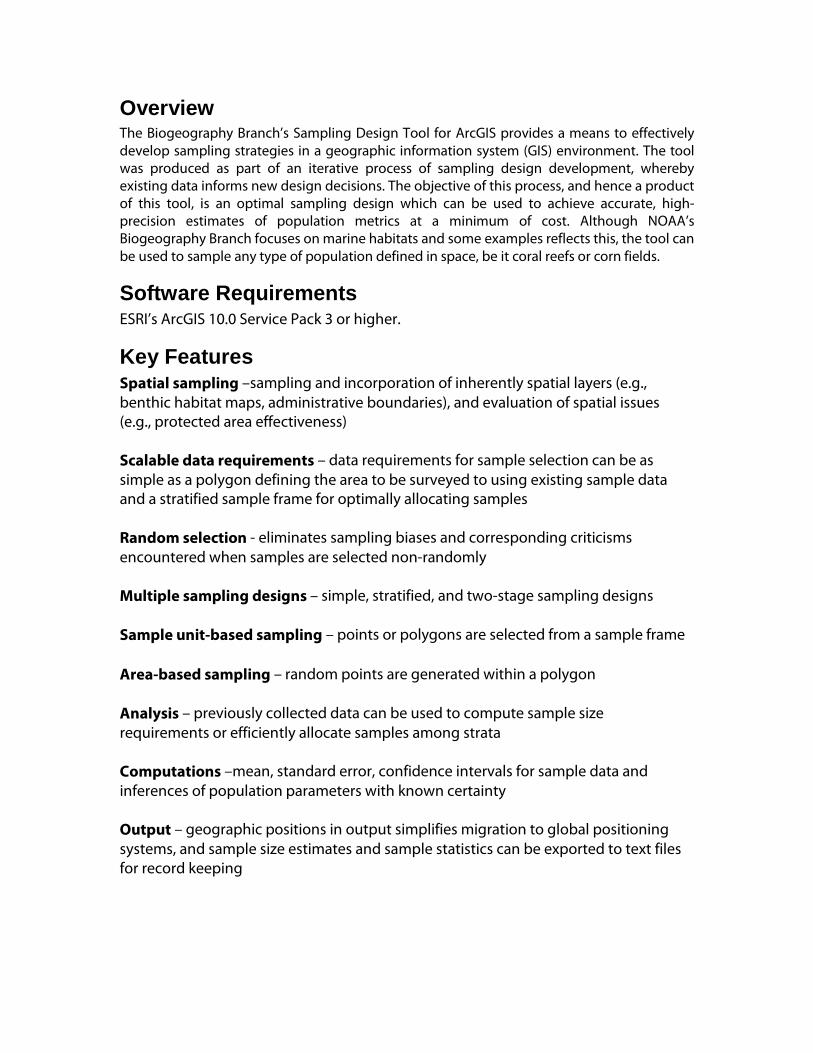
Overview The Biogeography Branch’s Sampling Design Tool for ArcGIS provides a means to effectively develop sampling strategies in a geographic information system (GIS) environment. The tool was produced as part of an iterative process of sampling design development, whereby existing data informs new design decisions. The objective of this process, and hence a product of this tool, is an optimal sampling design which can be used to achieve accurate, high-precision estimates of population metrics at a minimum of cost. Although NOAA’s Biogeography Branch focuses on marine habitats and some examples reflects this, the tool can be used to sample any type of population defined in space, be it coral reefs or corn fields.

Software Requirements ESRI’s ArcGIS 10.0 Service Pack 3 or higher.

Key Features Spatial sampling –sampling and incorporation of inherently spatial layers (e.g., benthic habitat maps, administrative boundaries), and evaluation of spatial issues (e.g., protected area effectiveness) Scalable data requirements – data requirements for sample selection can be as simple as a polygon defining the area to be surveyed to using existing sample data and a stratified sample frame for optimally allocating samples Random selection - eliminates sampling biases and corresponding criticisms encountered when samples are selected non-randomly Multiple sampling designs – simple, stratified, and two-stage sampling designs Sample unit-based sampling – points or polygons are selected from a sample frame Area-based sampling – random points are generated within a polygon Analysis – previously collected data can be used to compute sample size requirements or efficiently allocate samples among strata Computations –mean, standard error, confidence intervals for sample data and inferences of population parameters with known certainty Output – geographic positions in output simplifies migration to global positioning systems, and sample size estimates and sample statistics can be exported to text files for record keeping

Installation and Setup In a file manager, double click on the file SamplingTool_10.esriAddIn to start the ESRI Add-In Installation Utility. Once installed on your computer the Sampling Design Tool must be installed in ArcMap toolbar. Right-click an empty area of the toolbar and select “Customize” at the bottom of the menu. Next, select the “Commands” tab. Scroll down and select “Biogeography Branch” under the “Categories list”. Then drag “Sampling Design Tool” displayed in the right-hand pane to any space on your toolbar. To use the tool, click on the Sampling Design Tool button. The main console will open.

Create Point Samples Random points are commonly used to sample a population defined by an area on a map (e.g., political jurisdiction, marine protected area, habitat). By taking measurements at points distributed randomly throughout the population, an unbiased survey of the population can be undertaken. This procedure is a form of

area-based sampling and is aided by data in a GIS. The Sampling Design Tool offers 3 ways to generate point samples: simple random, stratified random and multi-stage random. The choice of which method to use will depend on survey objectives and types of available data. Random numbers to either create new points (or selecting random features) are generated using a seed value. If the same seed is used repeatedly, the same series of numbers is generated. If no value is entered into the following processes, a seed will be generated based of the computer’s clock. A seed should ideally be more than four digits. The Simple Random procedure generates randomly placed points within a population defined by a polygon dataset. This procedure is optimal when there is little information available for the population, covariates or spatial patterns of intended measurements. If the area for which random points will be assigned consists of multiple polygons, the distinct polygons are automatically dissolved together and treated as one. The Stratified Random procedure generates randomly placed points within mutually-exclusive subareas of a population, or strata. Strata are identified by choosing an attribute (column) in the sample frame’s attribute table which distinguishes polygons amongst different strata. All polygons with the same value are considered part of the same stratum. Several methods can be used to allocate points among strata. Users can set the number of points to each stratum themselves, assigned proportional to the area of each stratum (i.e. larger strata get more points) or assigned equally among all strata. If either of the two latter methods is used, the user must identify the total number of sample units to allocate. A stratified sample is superior to a simple random sample if a polygon dataset separates a heterogeneous population into internally homogenous groups (e.g., benthic habitat map). The Two-stage procedure samples in two simple random stages. First, a sample of primary sampling units (PSUs) is selected. PSUs must be defined by a polygon dataset. Then random points are placed in each selected PSU. The user selects the number or percentage of PSUs to be sampled and the number of points to be placed in each PSU. This procedure is generally used when the variance of a measured metric is highly variable at fine spatial scales. The output of all procedures is a point dataset. The user must select where the dataset will be saved. The attribute table of all output datasets will contain their X and Y geographic coordinates as defined by the data frame’s coordinate system. The results of using the option “Keep a minimum distance between points” will be dependent on the scale of the map, the distance and units chosen, and the timeout

period. If not all points could be created, a message box will show how many points were able to be randomly placed. Users may also export stratified sample allocations to a table for recordkeeping, for use in a statistical software package or to repeat the same allocation in the future. To use a saved allocation table the table must be imported. This table must be comma delimited with at least two columns, one designating distinct strata and one for corresponding stratum sample sizes.

Select Sample from Frame A sample can be selected from a sample frame (point, line or polygon dataset) using simple random or stratified random sampling. In these procedures, a selection set is created from the list of sampling units. The Simple Random procedure randomly selects a number or percentage of sample units. The Stratified Random procedure selects sample units from different strata. Strata are identified by choosing an attribute (column) in the sample frame’s attribute table. All sample units with the same value are considered part of the same stratum. Several methods can be used to allocate sample units among strata. Users can set the number of sample units to each stratum themselves, sample units can be assigned proportional to the area of each stratum (i.e. larger strata get more sample units) or sample units can be assigned equally among all strata. If either of the two latter methods are used the user must identify the number of sample units to allocate. A stratified sample is superior to a simple random sample if a polygon dataset separates a heterogeneous population into internally homogenous groups (e.g., benthic habitat map). For both Simple Random and Stratified Random procedures a dataset (i.e. permanent record) can be produced from the selection set by checking the “Export selected features” on the main console.

Analyze/Refine Sample Data A common procedure when gathering data for a monitoring program is to analyze existing data to refine the sample selection procedure. This process produces more-efficient sampling designs. An analysis of past data can suggest new strata, a more efficient sample allocation among strata, or the need for fewer (or more) samples to achieve a desired objective. To analyze existing sample data, choose the Analyze/Refine Samples option on the main console. Then select the appropriate sampling design (i.e. simple random or stratified random) and sample frame (polygon or point dataset), strata field (if needed; column in attribute table of sample frame), sample data layer (point dataset), and metric field (column in attribute table of sample data). The metric field corresponds to

a continuous numerical attribute and represents measurements taken from a population (e.g., fish abundance, coral size, invertebrate biomass). The Sampling Design Tool provides two main outputs: sample size requirements and sample data statistics. Sample statistics include the mean, standard error, coefficient of variation and upper and lower 95% confidence limits. The confidence interval is given by )( styszα± , where z is the critical value of a Normal distribution with 95% confidence (i.e. α = 0.05) and )( stys is the square root of the standard error. Note: population estimates are only valid if the appropriate sampling design is used. Statistics are calculated using computational methods presented in Cochran (1977). Please read Cochran’s (1977) Sampling Techniques for more information on analyses.

Sample size requirements are based on desired objectives. Users must select one of four analytical approaches, and a desired precision. The precision sets the amount of desired agreement among repeated measurements. Precision is set as a proportion (e.g., 0.1, 0.2, and 0.5), which correspond with a percentage (e.g., 10%, 20%, and 50%). If the chosen sample frame is a polygon dataset the user must also select whether the analysis is sampling unit-based or area-based. Sampling unit-based means records in the sample frame dataset are used to define sampling probabilities (this is the normal

way). Area-based sampling indicates polygon areas and user-defined measurement plot sizes are used to estimate sampling probabilities. Four distinct analytical approaches to examine sample variability are provided: Coefficient of variation, Confidence Interval (CI), t-test with various Type I errors, and t-test with various Type I and Type II errors (i.e. power analysis). The correct choice will depend on how the data will be analyzed. The coefficient of variation (CV) is a standardized measure of the standard error and represents sample variability. If CV is chosen as the analytical approach, the output reflects the sample size needed for the CV to equal the user-defined precision. This is the simplest analytical approach and does not require data to fit any model assumptions. A confidence interval is an interval estimate of a population parameter and is an alternative method of representing variability. By selecting precision and a confidence level (reciprocal of the Type I error rate) the user identifies the range of acceptable imprecision by a lower and upper bound. For instance, if precision is set to 0.10 and confidence level is set to 95%, the interval represented by +/- 10% of the sample’s mean would contain the population mean 95% of the time. Two different analytical approaches are provided when samples will be compared using t-tests. The first approach only incorporates a confidence level whereas the second also incorporates statistical power (reciprocal of the Type II error rate). The results are presented as a matrix of sample size requirements for several conventional confidence and power rates. These tests have statistical assumptions which must be met in order for results to be valid. Users also have the ability to investigate the impact of the finite population correction (FPC) by checking the corresponding checkbox. The FPC provides a reduction in standard error for sampling a greater proportion of the sample frame and consequently lessens sample size requirements. To help users identify affordable sampling designs they can enter the maximum sample size allowed below the sample size estimate results box. They can also check the highlight max value box and all sizes greater than what can be afforded are grayed out. The user can also manually set the sample size in the Choose Sample Size text box. A report of the analysis can be saved by clicking the “Export Statistics” button. This will save a text file for permanent records including, the data used, analytical selections (e.g., FPC, sample unit based), sample size requirements, population statistics and strata statistics.

Sample Allocation can be accomplished using proportional, optimal or user defined settings. The Optimal or Neyman allocation method uses the proportion of sample units and estimated variance with each stratum to allocate samples. Strata with more sample units and variance (i.e. heterogeneous) will receive more samples. This option is not available unless existing sample data is being analyzed, because it requires an estimate of stratum variance.

Acknowledgements Eric Finnen completed the first version of the Sampling Design Tool and laid the foundation for subsequent versions. Chris Caldow has provided guidance and support at every step of tool production.

Contacts Contact Ken Buja for questions on technical matters and Charles Menza for questions on sampling procedures. NOAA/NOS/NCCOS/CCMA Biogeography Branch 1305 East West Highway Silver Spring, MD 20910 Phone: (301) 713-3028

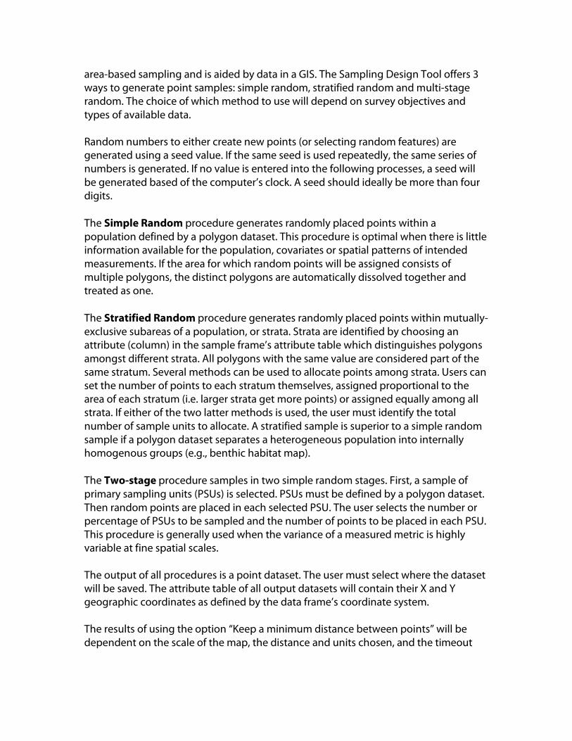
Example This example illustrates the iterative approach to sampling design development. Commonly, a sample frame is used to generate a simple random sample. This sample is used to collect measurements. The measurements are then analyzed to come up with an alternative design. The results are then used to develop an enhanced sampling design. This example describes this process and is divided into two parts. The first part describes the process of selecting a simple random sample. The second part describes the process of using this simple random sample to select an enhanced stratified random sample. 1.1 Choosing a simple random sample

1) To select a simple random sample a sample frame is needed. The frame can be a point, line, or polygon dataset. For this example the sample frame is a point dataset made up of a uniform distribution of points (Figure 1.1). The sample frame provides an unbiased representative coverage of the coral caps in the Flower Garden Banks National Marine Monument. Each point represents a potential measurement plot and all points represent the target population (e.g. sampling universe).

2) Select the Simple Random option under the Select Sample from Frame procedure. (Figure 1.2)

3) Check Export Selected Features to create a dataset of the results. (Figure 1) 4) Enter the sample frame data layer under Select sample frame. A sample will be

selected from this layer. Use the dropdown menu to select a dataset in the data frame or the folder browser to choose a dataset not in the data frame. (Figure 1.2)

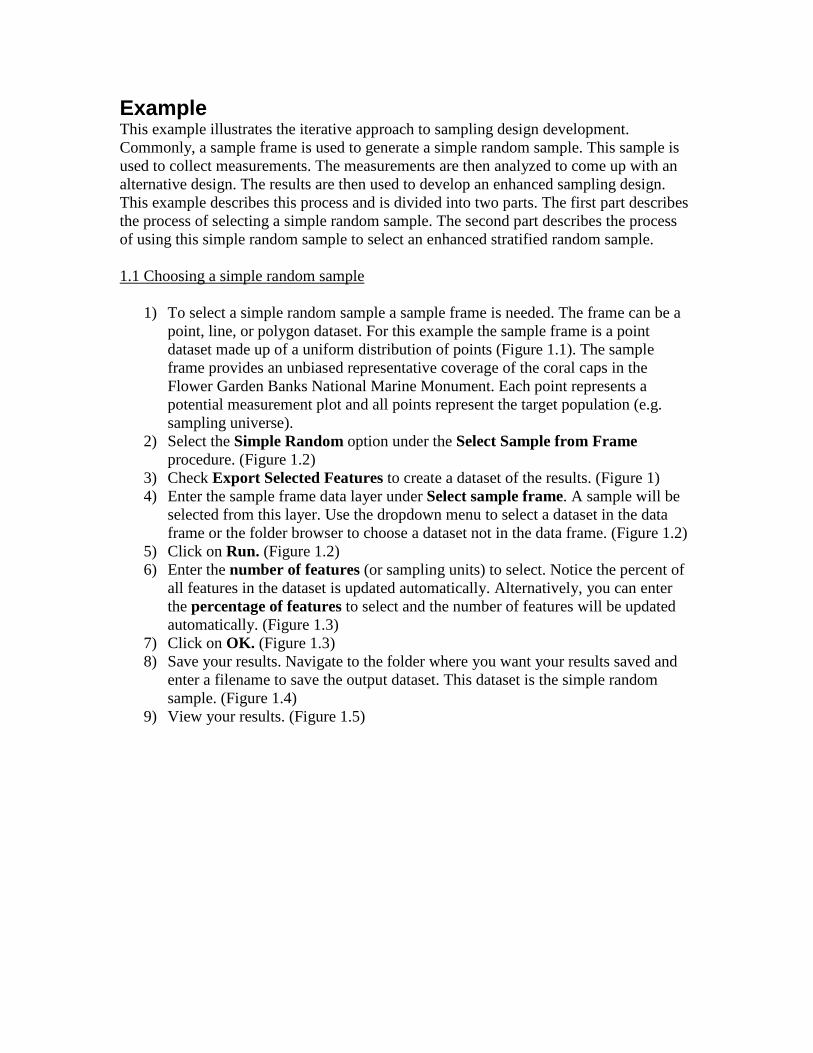
5) Click on Run. (Figure 1.2) 6) Enter the number of features (or sampling units) to select. Notice the percent of

all features in the dataset is updated automatically. Alternatively, you can enter the percentage of features to select and the number of features will be updated automatically. (Figure 1.3)

7) Click on OK. (Figure 1.3) 8) Save your results. Navigate to the folder where you want your results saved and

enter a filename to save the output dataset. This dataset is the simple random sample. (Figure 1.4)

9) View your results. (Figure 1.5)

Figure 1.1

Figure 1.2

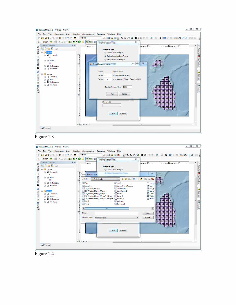
Figure 1.3

Figure 1.4

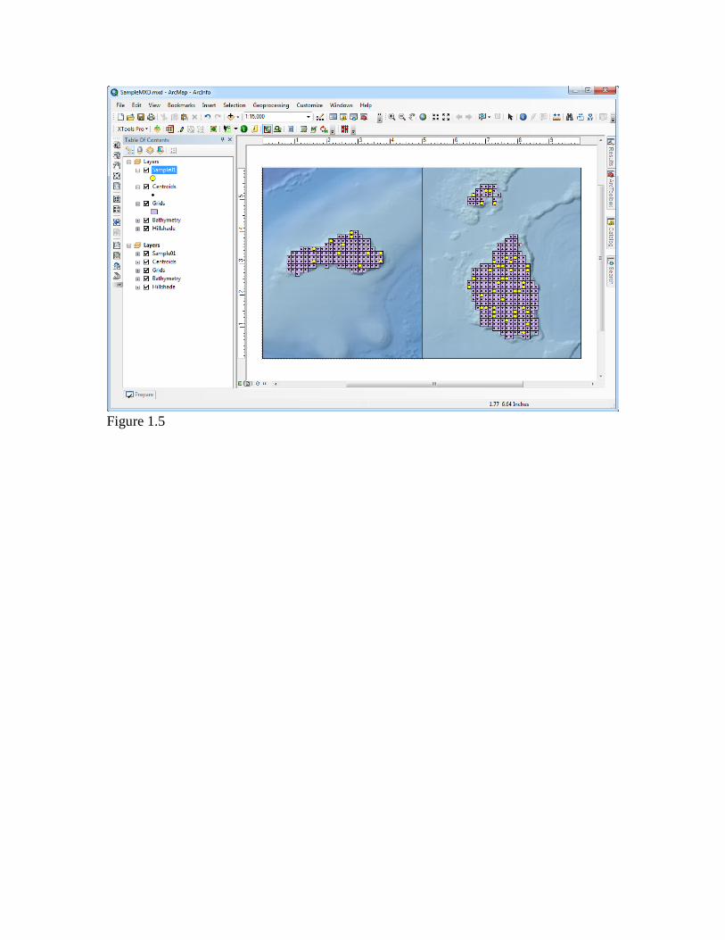
Figure 1.5

2.1 Refining Sample Selection using previously collected data

1) To refine sample selection, previous data and a sample frame are required. For this example, the simple random sample from the previous example is used with a continuous variable, “metric”, added to the attribute table. The sample frame has been divided according to the stratified sampling design defined in Section 2 of the report (StRS-composite) (Figure 2.1; EBHRD, EBHRS, EBLR, WBHRD, WBHRS, WBLR). The points in the figure are stratified and their strata are represented by the color of the surrounding squares.

2) Select the Stratified Random option under the Analyze/Refine Samples procedure. (Figure 2.2)

3) Select the sample frame data layer. Use the dropdown menu or folder browser to choose a point or polygon dataset. (Figure 2.2)

4) Enter the strata field used to define strata in the sample frame. The dropdown menu is populated using the sample frame’s attribute table. (Figure 2.2)

5) Select a sample data layer with previously collected data and which will be examined. This data should have been collected using the sample frame defined in step 4. (Figure 2.2)

6) Select a metric on which to perform analyses. The dropdown menu is populated using the sample layer’s attribute table. (Figure 2.2)

7) Click on Run. (Figure 2.2). 8) If needed, a message box will appear to describe any computational problems.

The user can fix these problems or decide to continue. 9) Choose the survey objective, the degree of precision and whether or not the

finite population correction will be used. (Figure 2.3) 10) If the degree of precision is modified, click on Recalculate 11) In this example, we want to know what sample size is required to obtain a

coefficient of variation of 20%. (Figure 2.3) 12) Sample size estimates to achieve the desired survey objective are shown in the

window to the upper right of the form. In some cases, numerous sample size requirements are provided to help the user identify variability. If a certain maximum sample size can be afforded, the sample size results can be highlighted to demonstrate those sample sizes below the maximum amount. The default maximum sample size is set at 100, but this can be edited. Check the Highlight maximum sample size box to use this feature. (Figure 2.3)

13) Unfortunately, we know that only a sample of 60 can be afforded. The allocation can be amended to by checking the Choose sample size feature and entering a sample size. (Figure 2.3)

14) Click on Allocate Samples (Figure 2.3) 15) Choose to allocate samples using the Optimal or Neyman allocation method.

(Figure 2.4) 16) (Optional) Add 3 extra sample units to each stratum. This will add a small buffer

in case a sampling unit allocated in Step 15 cannot be reached. Add extra samples by typing into the table. (Figure 2.5)

17) Click on Run. (Figure 2.4 or 2.5)

18) Save your results. Navigate to the folder where you want your output dataset saved and enter a filename.

19) View your results!

Figure 2.1

Figure 2.2

Figure 2.3

Figure 2.4

Figure 2.5