Sampling Distribution of&

the Central Limit Theorem

x

iClickerFill in the blanks: The sampling distribution of is the ___________ distribution of ____ for an SRS of a specified _______ from a population.

a. random, x, sb. normal, s, sc. normal, , s d. probability, , size

x

xx

Height Data for Our Class

• Suppose distribution of BYU heights has μ = 68.18 inches (~ 5’ 8”) and σ = 4.49 inches

• Someone says BYU’s incoming class for Fall 2014 will have a mean height larger than 68.18, based on a random sample of n=5 incoming freshman with = 69.5. What do you think?– What if the came from a sample with n=16?

n=100?x

x

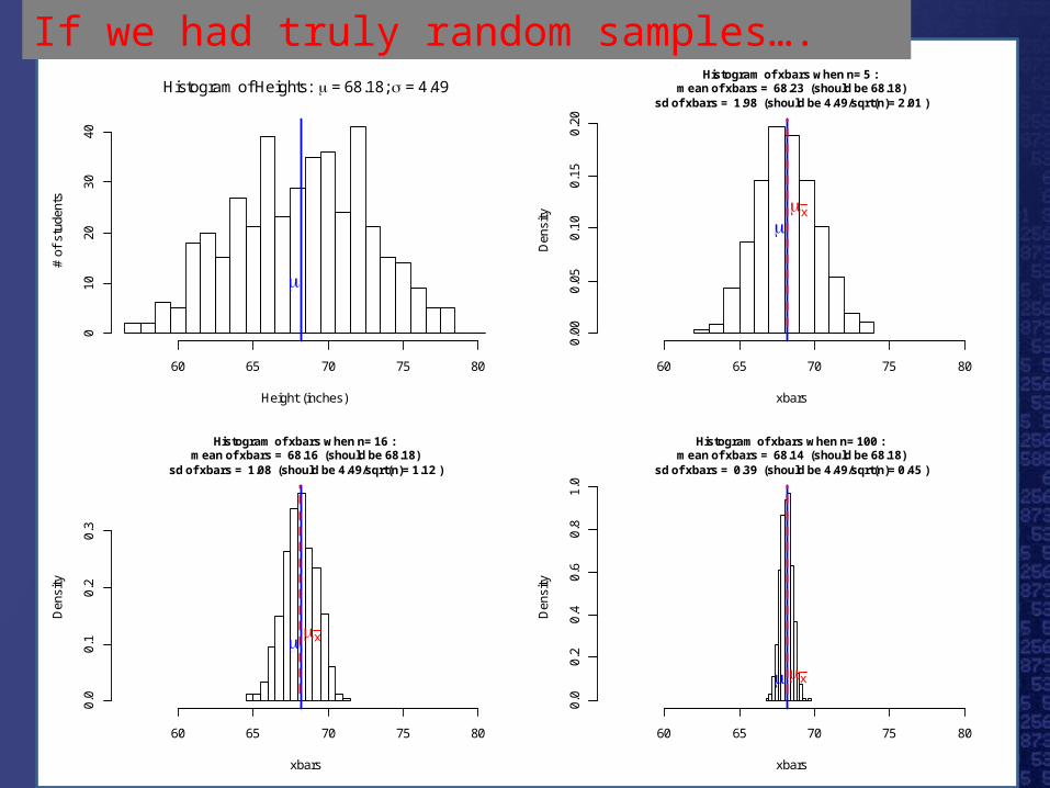
If we had truly random samples….Histogram of Heights: = 68.18; = 4.49

Height (inches)

# of

stu

dent

s

60 65 70 75 80

010

2030

40

Histogram of xbars when n= 5 : mean of xbars = 68.23 (should be 68.18)

sd of xbars = 1.98 (should be 4.49/sqrt(n)= 2.01 )

xbars

Den

sity

60 65 70 75 80

0.00

0.05

0.10

0.15

0.20

x

Histogram of xbars when n= 16 : mean of xbars = 68.16 (should be 68.18)

sd of xbars = 1.08 (should be 4.49/sqrt(n)= 1.12 )

xbars

Den

sity

60 65 70 75 80

0.0

0.1

0.2

0.3

x

Histogram of xbars when n= 100 : mean of xbars = 68.14 (should be 68.18)

sd of xbars = 0.39 (should be 4.49/sqrt(n)= 0.45 )

xbars

Den

sity

60 65 70 75 80

0.0

0.2

0.4

0.6

0.8

1.0

x

Next…• What if we don’t have the whole population to

simulate from?• What if we don’t have 600 Stat 121 students

willing to calculate values based on 600 different samples? [applet]

– What if we only have time for one sample of size n=35 (BYU students), and we get 6.9 hours as an average number of TV hours per week? Can we say that BYU students’ mean viewing time is significantly less than the national average of 10.6 hours for college students? (σ=8.0) What if we knew somehow that the samp. dist. for is normal?

x

x

Amazing Facts About Sampling Distribution of

mean of sampling distribution of always , m(mean of the population) regardless of n

standard deviation of sampling distribution of always

[applet]

x

x

x

/ n

Even More Amazing Fact

if n “large” (30 is ample), shape of sampling distribution of is close to the normal curve– shape of original population distribution

doesn’t matter!– mathematically, this fact called central

limit theorem

x

I know of scarcely anything so apt to impress the imagination as the wonderful form of cosmic order expressed by the "Law of Frequency of Error [Central Limit Theorem].” The law would have been personified by the Greeks and deified, if they had known of it. It reigns with serenity and in complete self-effacement, amidst the wildest confusion. The huger the mob, and the greater the apparent anarchy, the more perfect is its sway. It is the supreme law of Unreason. Whenever a large sample of chaotic elements are taken in hand and marshaled in the order of their magnitude, an unsuspected and most beautiful form of regularity proves to have been latent all along.

-- Sir Francis Galton

Demo

view sampling distribution applet

Implications of Central Limit Theorem

If n is large (bigger than 30-ish will do), then:• We can calculate probabilities on obtained

from random samples of “any” population (even highly non-Normal populations).

E.g., regardless of population distribution shape: – 68% prob. that next will be within

of m– 95% prob. that next will be within

of m– 99.7% prob. that next will be within

of m

x

x

x

/ n

/2 n

/3 n

x

iClickerConsider taking a random sample of size 49 from a left-skewed population with mean 80 and standard deviation 7. There is a 68% chance that will be between _____ and ____.

a. 73, 87b. 66, 94c. 79, 81d. 77, 83

x

Special Case

If population exactly follows the normal distribution…

Special Case

…then sampling distribution of is exactly the normal curve for any n (even small values)

x

Summaryprobability distribution of (or “sampling

distribution of ”) for SRS of size n from population with mean μ and st. dev.

mean of dist. of = μ

standard deviation of dist. of =

approximately normal (if population not normal and n large) or exactly normal (if population normal )

Center

Spread

Shape

x

x

x / n

x

Summary

More Implications

• standard deviation of always less than

• standard deviation of reduced by factor of

• to cut standard deviation of in half, increase n 4-fold

• to cut standard deviation of to one-fourth, increase n 16-fold

x

x/1 n

x

x

(assuming n > 1)

iClickerConsider taking a random sample of size 64 from a right-skewed population with mean m and standard deviation s. The sampling distribution of has standard deviation ____.

a. s/64b. s/32c. s/16d. s/8e. Impossible to say…n isn’t big

enough to calculate

x

Even More Implications

If n is large:• can use the standard normal table (Table

A) or normal probability function to compute probabilities about

• don’t have to know the shape of the population distribution to compute probabilities about

• don’t have to simulate process a bunch of times to compute probabilities

x

x

Example 1

BYU Creamery sells bottles of chocolate milk containing μ = 1.0877 lb of milk with = 0.015 lb. The weights are normally distributed. What is the probability that a randomly selected bottle weighs more than 1.1 lb?

Example 11. Draw picture

2. Compute z-score

3. Look up z-score in table A to get probability

Example 2

BYU Creamery sells bottles of chocolate milk containing μ = 1.0877 lb of milk with = 0.015 lb. The weights are normally distributed. What is the probability that for a random sample of 8 bottles of chocolate milk exceeds 1.1 lb?

x

Example 21. Draw picture

2. Compute z-score

3. Look up z-score in table A to get probability

Example 3

Closing prices of stocks have a right skewed distribution with μ = $26 and = $20. What is the probability that the closing price of a randomly chosen stock is less than $15?

Example 31. Draw picture

2. Compute z-score

3. Look up z-score in table A to get probability

Example 4

Closing prices of stocks have a right skewed distribution with μ = $26 and = $20. What is the probability that for a random sample of n = 10 closing stocks is less than $15?

x

Example 41. Draw picture

2. Compute z-score

3. Look up z-score in table A to get probability

Example 5

Closing prices of stocks have a right skewed distribution with μ = $26 and = $20. What is the probability that for a random sample of n = 32 closing stocks is less than $15?

x

Example 51. Draw picture

2. Compute z-score

3. Look up z-score in table A to get probability

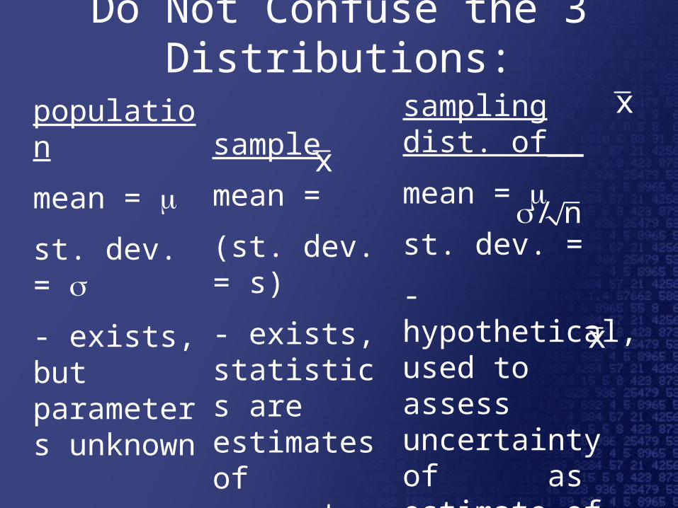
Do Not Confuse the 3 Distributions:

population

mean = m

st. dev. = s

- exists, but parameters unknown

sample

mean =

(st. dev. = s)

- exists, statistics are estimates of parameters

sampling dist. of__

mean = m

st. dev. =

- hypothetical, used to assess uncertainty of as estimate of m

x

x

x

/ n

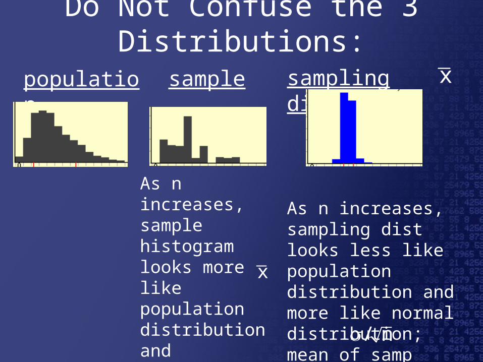
Do Not Confuse the 3 Distributions:

population sample

As n increases, sample histogram looks more like population distribution and gets closer to μ

sampling dist. of__

As n increases, sampling dist looks less like population distribution and more like normal distribution; mean of samp dist is ALWAYS μ and sd is ALWAYS

x

x

/ n

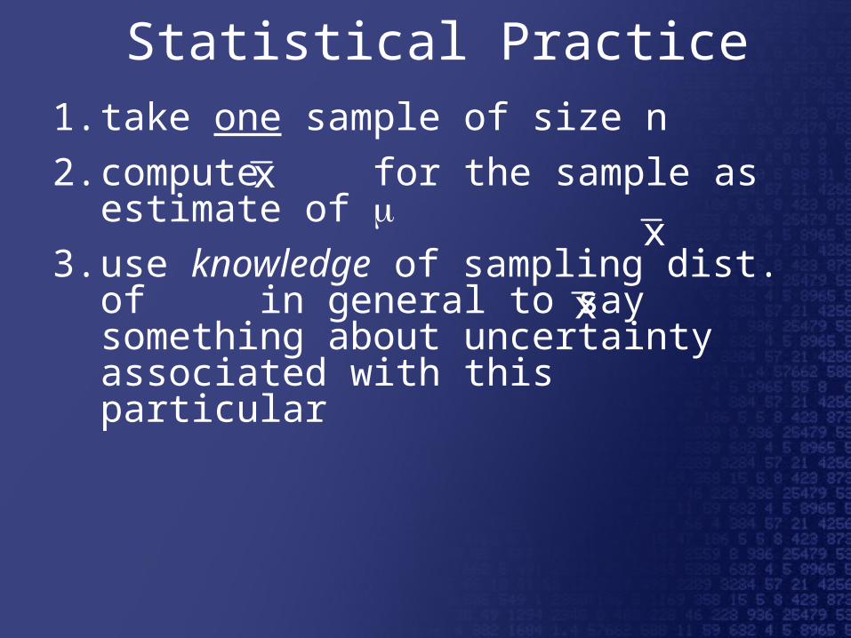
Statistical Practice1. take one sample of size n2. compute for the sample as estimate of m 3. use knowledge of sampling dist. of in

general to say something about uncertainty associated with this particular

xx

x

Statistical PracticeExample:

Sample of size n=35 (BYU students), and we get 6.9 hours as an average number of TV hours per week. Can we say that BYU students really watch less than the national average of 10.6 hours for college students? (σ=8.0) That is, what’s the chance of randomly getting an less than 6.9 hours if m really is equal to 10.6?

x

Vocabulary

Central Limit TheoremSimple Random SamplePopulation DistributionSampling Distribution of Standard Deviation of

xx