samuel selikoff neoclassical consumer theory samuel selikoff abstract: neoclassical consumer theory...

Understanding Neoclassical Consumer Theory

Samuel Selikoff

Abstract: Neoclassical consumer theory forms the core of modern economics. Its evolution

culminated in the early half of the 20th century with the development of indifference curve

analysis, which allegedly bridged the gap between the undeniable fact of ordinal utility and the

application of the revered methods of differential calculus to economics. Widespread acceptance

of the theory was inevitable, for economists who had pointed to the success of calculus in

physics were now justified in employing it themselves. Today, economists of all types conduct

research under the principles of neoclassical consumer theory.

But modern economic theory, including the the theory of the consumer, is not universally

cherished. Austrian economists in particular have criticized almost every aspect of neoclassical

consumer theory. Unfortunately, these critiques are scattered and incomplete, and some even

misrepresent the neoclassical position completely. This paper attempts to rectify this. The first

section is a charitable exposition of neoclassical consumer theory, in which the reader will learn

which assumptions are essential to the framework, as well as many of the key differences

between the neoclassical and Austrian approaches. The second section offers a brief discussion

of the utility function approach to neoclassical consumer theory, and points out several common

misunderstandings that stem from that approach. The third section concludes by critiquing the

neoclassical position. Upon completion of this paper, the reader will have a better understanding

of what neoclassical consumer theory says, what it does not say, and its many flaws.

Samuel Selikoff ([email protected]) studied graduate economics at Boston College. The author would like to thank Robert Murphy and Joseph Salerno, and particularly Jeffrey Herbener for many useful conversations, as well as the Mises Institute for financial support. All errors contained are his own.

mailto:[email protected]

mailto:[email protected]

Table of Contents

1 The Neoclassical Formulation! 31.1 Preferences 3

1.2 Assumptions 6

1.3 Indifference Curves and the MRS 13

1.4 Consumer Choice 16

1.5 Consumer Demand 24

2 Utility Functions! 282.1 Utility Functions and the Representation Theorem 28

2.2 The Utility Maximization Problem 38

2.3 Marginal Utility 39

2.4 Uniqueness, Ordinality and Cardinality 41

3 Critiques! 443.1 On Preferences 45

3.2 On Rationality and Continuity 54

3.3 On Convexity 58

3.4 On Marginal Utility 61

3.5 On Money 65

3.6 On Abstraction 77

3.7 On Econometrics 79

Conclusion! 93

References! 95

2

1 The Neoclassical Formulation

1.1 Preferences

Neoclassical consumer theory begins its analysis by considering individuals as consumers

only i.e. as purchasers of consumer goods. This is not to deny that individuals may also act as

producers in the market, but this function is ignored in consumer theory.

The consumer is assumed to be faced with a choice from among many consumption bundles.

This means our consumers aren’t choosing whether to buy six or twelve eggs, for example, but

instead they are choosing between two bundles a and b, where bundle a has six eggs and bundle

b has twelve. Formally, each consumption bundle is a vector of n different goods

x = x1,..., xn( )

where x1 is the amount of good 1 contained in the bundle, x2 is the amount of good 2, and so on.

Since each bundle is a vector, it can be equivalently thought of as a mathematical point in n-

dimensional space. The set of all bundles is X.

The consumer is said to have preferences over the set X, where preferences are defined as

follows:

Preferences

The consumer’s preferences between bundles in X are denoted

x y

which means “the consumer thinks bundle x is at least as good as bundle y.”

If both x y and y x , the consumer is said to be “indifferent” or have “no preference”

between x and y, denoted x ~ y .

If x y but not y x , the consumer is said to “strictly prefer” x to y, denoted x y .

The key word in this definition is thinks. The assumption is referring to the consumer’s

psychological beliefs or feelings, feelings which then determine his choice behavior. Thus, while

the consumer bases his actions on his preferences, the two exist independent of one another. The

neoclassical economist understands and acknowledges this.1

It’s important to note that this is entirely different from the Austrian conception of

preferences. Neoclassical economics takes as its starting point feelings that influence action, and

calls these things preferences, while Austrian economics takes action itself as its starting point,

and conceives of preferences as facts of action.2 Austrians often mention that indifference can

never be the basis for action, and thus the concept has no place in economics. While true from

the Austrian perspective, this criticism does not apply to neoclassical economics, where

The Neoclassical Formulation

4

1 As Mas-Collel (1995, p. 5) states (emphasis added),“The theory [of consumer behavior] is developed by first imposing rationality axioms on the decision makerʼs preferences and then analyzing the consequences of these preferences for her choice behavior (i.e. on decisions made).”

2 As Hulsmann (1999, pp. 3-4) writes,“The Austrians explain the realized elements of an action (observed behavior) in terms of non-realized elements of the same action... By contrast, neoclassical economists seek to explain observable phenomena (behavior) in terms of other observable phenomena (behavior of other persons, physical conditions of action) or of psychological phenomena (ʻdegrees of want-satisfactionʼ).”

For more on this, see Rothbard (2009, Chapter 4, Section 9).

preferences are thoughts, and where indifference is equivalent to someone saying or thinking, “I

don’t care which movie we watch.” It describes a psychological state of mind, and there is

nothing de facto absurd or contradictory about it. Whether it is relevant for explaining economic

phenomena is, of course, an entirely different question. For now, we simply want to state that

psychological indifference is a logical possibility - even if praxeological indifference is not.

Now we may ask, do real individuals even have preferences, in the sense defined by

neoclassical economics? It does seem like we can ask ourselves whether we like one thing more

than another, or whether we have no preference for either. But we must also remember that the

‘things‘ between which consumers have preferences are bundles. When was the last time you

asked yourself if you preferred a bundle containing three bananas and two apples to one

containing one banana and four apples? It seems like people never ask themselves questions of

this sort. Admittedly, a neoclassical economist could say that when a consumer goes to the store

and decides how many bananas and how many apples to purchase, his choice problem can be

reframed in the above way i.e. as a selection between bundles with varying amounts of the two

goods in them. Certainly this is true, although it seems like an unnecessary complication, and one

which doesn’t capture the reality of the consumer’s decision.

In any case, it seems like people can indeed have preferences so defined. Certain

psychological feelings are ruled out, such as, “the bundles x and y are not comparable”; but we

can at least conceive of everyone potentially having the preferences defined above. This is an

important point because, as we shall soon see, neoclassical consumer theory does exclude certain

individuals from its analysis. So far, though, no individuals are being excluded outright, based

solely on this definition of preferences.


5

In sum, the preference relation is the primitive concept of Neoclassical consumer theory. It

is an ordinal ranking rule, albeit one that allows for ties.

Now that we have defined the consumer’s preference relation, we can introduce the concept

of indifference sets. These are simply sets of bundles between which the consumer has no

preference, or, equivalently, between which he is indifferent. Formally:

Indifference Sets

The indifference set containing the bundle x is the set

y ∈X : y ~ x{ }

It’s important to realize that (1) an indifference set is a locus of points (bundles), (2) the

consumer is, by definition, indifferent between each of these points, and (3) this last fact derives

solely from the preference relation. Also, note that an indifference set is defined in terms of a

specific bundle x.

When consumption bundles have only two goods in them, indifference sets can be

represented graphically in two-dimensional Euclidean space. These indifference sets take many

shapes, depending on the consumer’s preference relation. This graphical analysis is generally

used to explain the neoclassical framework, so we will make use of it; however, it does not

change the meaning of anything that has already been said.

1.2 Assumptions


6

We will now discuss some of the standard assumptions made on a consumer’s preference

relation. All the results we develop based on two-good consumption bundles generalize to an n-

good case, though the details are beyond the scope of this paper.

The first two conditions imposed on our consumer’s preference relation are

Completeness

For any two consumption bundles x and y in X, either x y , y x , or both (the

consumer is indifferent between the two).

Transitivity

For any three consumption bundles x, y, and z in X, if x y and y z , then x z .

A consumer whose preferences satisfy completeness and transitivity is said to be rational.3

Are preferences in the real world complete? The answer clearly depends on the definition of

the set X, that is, on which bundles the consumer is considering. If the set X is sufficiently

restricted, it seems that any person’s preferences would be complete. In forming a general theory

of prices, however, the set X typically includes all possible bundles, leaving open the possibility

that some consumers’s preferences are not complete. Indeed, as Mas-Collel (1995, p. 6) states,

“The strength of the completeness assumption should not be underestimated.

Introspection quickly reveals how hard it is to evaluate alternatives that are far


7

3 The definition of rationality sometimes also includes the condition of reflexivity: for all x ∈X , x x .

from the realm of common experience. It takes work and serious reflection to find

out one’s own preferences. The completeness axiom says that this task has taken

place: our decision makers make only meditated choices.”

So completeness is really a statement about the psychological awareness of the consumer. It is

clear from the above quote that some (perhaps many) consumers do not meet this condition, and

are thus ruled out of the analysis.

What about the assumption of transitivity 4? One of its purposes is to rule out intransitive

cycles in the consumer’s preferences. For example, suppose the consumer’s preferences are

apple orange, orange banana, banana apple

Then, if the consumer were faced with the set (apple, orange, banana), he would not be able to

make a choice; for no matter what he chooses, there is always something better. The transitivity

assumption thus appears reasonable on its surface.

However, transitivity certainly can be violated. A common example offered by standard

textbooks concerns just imperceptible differences5. Suppose an individual is indifferent between

one room with a temperature of 70°and another with a temperature of 70.5°. The temperature

difference is too slight for him to prefer one or the other. Suppose further that he is indifferent

between a 70.5° room and a 71° room; a 71° room and a 71.5°; and so on, up to 89.5° and 90°

rooms. By transitivity, since the individual is indifferent between all the rooms, then he should be

indifferent between the 70° room and the 90° room. However, when considering a 70° room and


8

4 As Mises points out (Human Action, Chapter 5, Section 4), transitivity only applies to systems of thought, and not action. But as the neoclassical concept of preferences is a system of thought, transitivity is applicable.

5 Cf. Mas-Collel (1995), pg. 7.

an 90° room, we can easily imagine the individual preferring the 70° room. In this example, then,

preferences violate transitivity. The individual cannot have both 70° ~ 70.5°~...~90° and

70° 90° . So just as with completeness, we see that the transitivity assumption excludes some

consumers from the analysis. Mas-Collel (1995, p. 6) echoes this claim:

“Transitivity is also a strong assumption, and it goes to the heart of the concept of

rationality… As compared to the completeness property, however, it is also more

fundamental in the sense that substantial portions of economic theory would not

survive if economic agents could not be assumed to have transitive preferences.”

In addition to the rationality assumptions, a monotonicity assumption is usually imposed on

the consumer. Stated broadly, the assumption says that “more is better,” meaning the consumer

will prefer bundle a to bundle b whenever bundle a has more of at least one of the goods from

bundle b in it, while having no less of any other6.

Next, a continuity assumption is imposed, which has to do with sequences of bundles:

Continuity

The preference relation is preserved under limits. In other words, for two infinite

convergent sequences of bundles

xk{ }

k=1

∞

and yk{ }

k=1

∞


9

6 This particular version of the “more is better” assumption is called strong monotonocity. The weaker assumption of local nonsatiation actually suffices for most of the neoclassical results we discuss, although it is more technical. The use of strong monotonicity doesnʼt affect our analysis. Cf. Mas-Collel (1995, pp. 42-43).

whose limits are x* and y* respectively, if x

k yk for all k, then x* y* .

This assumption, as its name suggests, ensures that indifference sets graphed in two-space will

be continuous. Thus, under the assumption of continuity, indifference sets will be indifference

curves; that is, the set of bundles over which the consumer is indifferent can be drawn as a

curve7.

Assuming indifference sets exist, the question of whether or not they are continuous seems

an impossible one to answer. Humans never even consider decision-making on an infinitesimal

level - for example, choosing between bundles with 1.40285 units of a car - so continuity

certainly cannot be empirically verified. Most neoclassical economists probably see this as an

approximating assumption, albeit one that sacrifices little economic significance.

There is one final assumption that relates to how preferences affect a consumer’s willingness

to substitute one good for another. To motivate this assumption, consider the following. First,

let’s say you have three pieces of pizza and two cans of soda. If I were to take one piece of pizza

away from you, how many cans of soda would you need to be indifferent between your new and

old bundles? Remember, this is purely a hypothetical, mental question. Let’s say you answer

“two cans” to my question. Then, the neoclassical economist would say that the rate at which

you’re willing to substitute pizza for soda is 2:1 (two-to-one).

Of course, the Austrian may protest, and say that if you were actually willing to make the

exchange (i.e. if you actually did exchange two sodas for one pizza), it must have meant that you


10

7 Although an indifference curve is usually associated with a representative utility function, itʼs important to understand that the curve is still just a locus of points. Itʼs better to think of the curve as a set of bundles, rather than as the level set of a specific utility function. This will be elaborated on in the next chapter.

preferred the latter bundle to the original. This is certainly true - but it is irrelevant for what the

neoclassical economist is describing. Remember that for him, preferences exist inside of our

minds. The “rate at which you’re willing to exchange” is simply your answer to question posed

above. It has nothing to do with action.

Now, we said the rate at which you were willing to exchange pizza for soda was 2:1. Notice

that your answer depended on what your starting bundle was. In our case, it was the bundle

(three pizzas, two sodas). Suppose now that you have the new bundle (two pizzas, four sodas),

which we already know you ‘value’ the same as the original bundle, by the paragraph above. We

can again ask the same question, namely, if I were to take yet another piece of pizza away, how

many cans of soda would you need to remain indifferent between this new bundle and your

current bundle? Let’s say your new answer is “three cans.” This means the rate at which you’re

willing to exchange pizza for soda is now 3:1. Thus, we see that the amount of soda you require

to ‘compensate’ you for successive unit losses of pizza varies based on how much of each good

you have. Of course, it doesn’t have to change - but the point is, it can.

This discussion leads us to a convexity assumption. Intuitively, if a consumer has convex

preferences, it means

“...from any initial consumption situation x, and for any two commodities, it takes

increasingly larger amounts of one commodity to compensate [him] for

successive unit losses of the other.” (Mas-Collel 1995, p. 44)

Thus, the preferences described in the previous paragraphs were in fact convex, since the amount

of soda required to compensate the consumer for successive unit losses of pizza was increasing:


11

for his first pizza he was happy with two extra sodas, while for his second pizza he needed three

extra sodas. Another way to think of convexity is that consumers will prefer more diverse

bundles of goods (the two interpretations are equivalent).

Formally, the assumption is:

Convexity

The preference relation is convex if for every x ∈X , the set of bundles at least as

good as x

y ∈X : y x{ }

is a convex set. That is, if y x and z x , then

α y + 1−α( ) z x

for any α ∈ 0,1⎡⎣ ⎤⎦ . It is strictly convex if the above implies

α y + 1−α( ) z x

As Mas-Collel (1995, p. 44) goes on to say, one can easily imagine situations where the

convexity assumption is unreasonable. For example, I may prefer a glass of milk or a glass of

orange juice to half a glass of each. Yet for now, we assume that the preference relation is

(strictly) convex.


12

1.3 Indifference Curves and the MRS

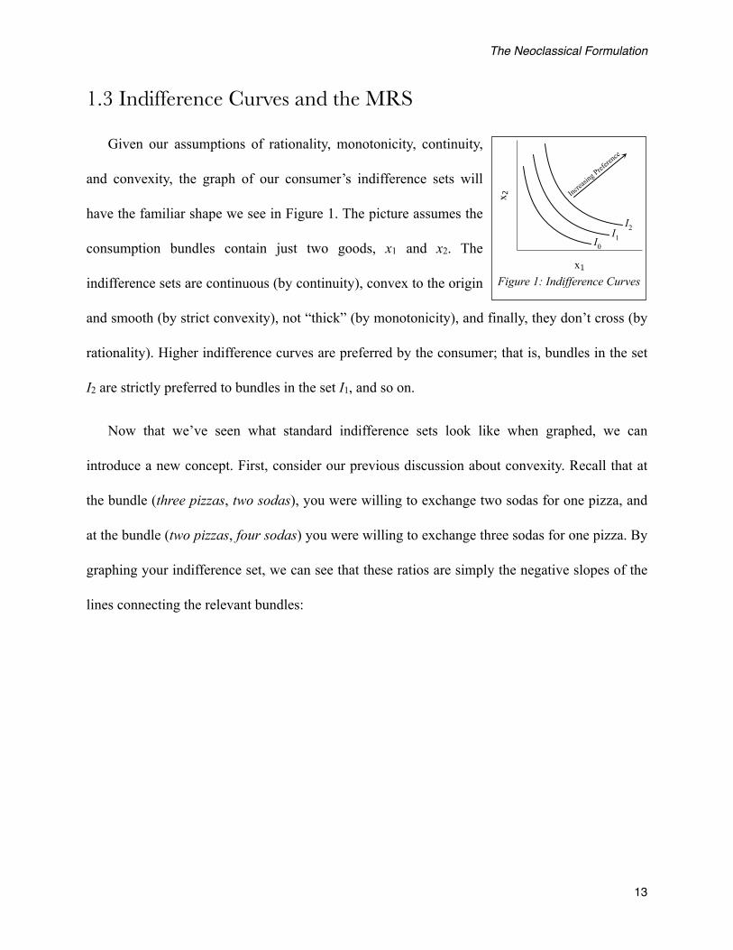
Given our assumptions of rationality, monotonicity, continuity,

and convexity, the graph of our consumer’s indifference sets will

have the familiar shape we see in Figure 1. The picture assumes the

consumption bundles contain just two goods, x1 and x2. The

indifference sets are continuous (by continuity), convex to the origin

and smooth (by strict convexity), not “thick” (by monotonicity), and finally, they don’t cross (by

rationality). Higher indifference curves are preferred by the consumer; that is, bundles in the set

I2 are strictly preferred to bundles in the set I1, and so on.

Now that we’ve seen what standard indifference sets look like when graphed, we can

introduce a new concept. First, consider our previous discussion about convexity. Recall that at

the bundle (three pizzas, two sodas), you were willing to exchange two sodas for one pizza, and

at the bundle (two pizzas, four sodas) you were willing to exchange three sodas for one pizza. By

graphing your indifference set, we can see that these ratios are simply the negative slopes of the

lines connecting the relevant bundles:

Figure 1: Indifference Curvesx1

x 2

I1

Increasi

ng Prefere

nce

I0

I2


13

Pizza

Soda

7

4

22 sodas

3 sodas

1 2 3

A

B

C

Figure 2: Movement Along an Indifference Curve

Between bundles A and B, the slope is -2 (the ratio was 2:1), and between bundles B and C, the

slope is -3 (the ratio was 3:1). As we can see, this slope will decrease (increase) as the amount of

pizza the consumer has decreases (increases). These results come from the convexity

assumption. Note that the units of both the ratios and the slopes are “sodas per pizza”.

Now, in our previous discussion, we asked how many sodas you would need in order to

remain indifferent if your stock of pizza changed by one unit. We can alter the question slightly,

and ask: at a certain starting bundle, for a tiny (or marginal8) change in your stock of pizza, how

many sodas would you need to stay indifferent? Just as in the above cases, your answer will

equal the negative slope of the line connecting your original bundle to the new bundle9.

However, for tiny changes in your stock of pizza (i.e. as the change approaches zero), the slope


14

8 In Austrian economics, the term marginal always refers to a single, discrete unit. This is not true in neoclassical economics, where the term usually means infinitesimal (as it does in the current context).

9 This is true by construction. There is no graphical trickery going on here; the graph just represents whatʼs already true, based on the given preference relation.

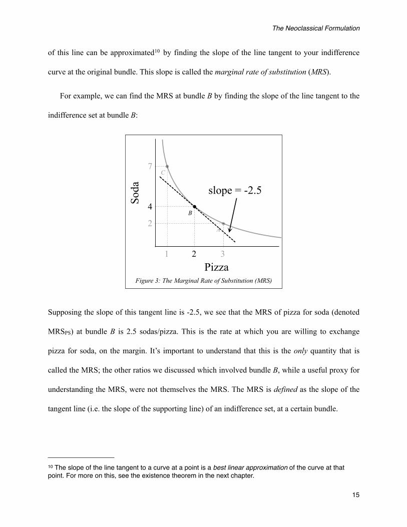
of this line can be approximated10 by finding the slope of the line tangent to your indifference

curve at the original bundle. This slope is called the marginal rate of substitution (MRS).

For example, we can find the MRS at bundle B by finding the slope of the line tangent to the

indifference set at bundle B:

Pizza

Soda

7

4

2

1 2 3

B

C

A

slope = -2.5

Figure 3: The Marginal Rate of Substitution (MRS)

Supposing the slope of this tangent line is -2.5, we see that the MRS of pizza for soda (denoted

MRSPS) at bundle B is 2.5 sodas/pizza. This is the rate at which you are willing to exchange

pizza for soda, on the margin. It’s important to understand that this is the only quantity that is

called the MRS; the other ratios we discussed which involved bundle B, while a useful proxy for

understanding the MRS, were not themselves the MRS. The MRS is defined as the slope of the

tangent line (i.e. the slope of the supporting line) of an indifference set, at a certain bundle.


15

10 The slope of the line tangent to a curve at a point is a best linear approximation of the curve at that point. For more on this, see the existence theorem in the next chapter.

When will the MRS exist? Generally, whenever the tangent line to a bundle exists. Given our

assumptions of continuity and strict convexity, we can see that every bundle along our

indifference set will have a tangent line. For this reason, neoclassicals often refer to preferences

that yield indifference sets that look like the ones we’ve drawn above as desirable or well-

behaved preferences. The existence of the MRS is important, because it is a critical part of

demand theory, as we shall soon see. If an indifference set has kinks, there will be bundles which

do not have an MRS11. The MRS will also generally not exist if the assumption of continuity is

dropped, such as when dealing with preferences between bundles of discrete units of goods.

Consumer demand can still be determined in such cases, albeit using a different method. Since

the MRS method is the most commonly used method in neoclassical demand theory, however, it

is the method on which we will focus our analysis.

Is the MRS real? Some economists maintain that it actually exists in our minds, some say it is

only a rule of thumb, and others treat it exclusively as a pedagogical device. Most, however,

probably see the MRS as a simplifying tool that lets us avoid the complexities of discrete

analysis, while still producing more or less similar results.

Finally, it needs to be stressed that the MRS is a property of the preference relation. Later we

will see that we can find the MRS using utility functions; but this does not change the fact that

the MRS derives solely from the underlying (ordinal) preference relation.

1.4 Consumer Choice


16

11 A common example of preferences that have kinked indifference sets is Leontief preferences, also known as perfect complements. For more on this, see Mas-Collel (1995, p. 49).

Now that we have established the fundamental axioms of the consumer’s preference relation,

we can turn to how it determines his choice behavior in the marketplace. In the previous section

we saw how a consumer’s preferences yielded his indifference curves, which were then used to

find his marginal rates of substitution at various consumption bundles. These rates are key in

explaining how the consumer chooses which bundle of goods to purchase, given his income and

an array of market prices.

First, it’s important to understand that the consumer’s choice is set up as a static problem.

This means that the consumer goes to a store with a given amount of money he earned from

work, takes the prices in the store as given, and decides how much of each good to buy. The

reason this is a static problem is because the consumer’s income and the store’s prices are taken

as exogenous parameters by the consumer i.e. as a given. Neoclassical economists can specify

several ways in which the actual price could be set; but what’s important for the current

discussion is that when a consumer walks into the store, he sees certain prices for different

goods, and then he uses these prices and his income to make his consumption decisions12.

Austrians have often criticized this particular idea, the idea that consumers take prices as

exogenous or given (also known as the price-taking assumption). Austrians point out that prices

are determined by both supply and demand, and that therefore to argue the consumers’ decisions

presuppose the very prices their decisions affect is to argue in a circle. The solution to this

misunderstanding is to recall how the mainstream conceives of preferences and consumer choice.

A consumer’s choice behavior is a result of his subjective, psychological feelings about various

bundles of goods. It is perfectly valid to stipulate that an individual consumer feels as if his own


17

12 In dynamic models, individuals can choose their labor output. For them, income becomes an endogenous or choice variable.

behavior will have no affect on the price of a good he is buying - even if it actually does. There

seems to be nothing logically contradictory about this; yet, this is all the neoclassical economist

is claiming. Now of course, an Austrian may say that our job as economists is not to explain why

certain people behave the way they do, but rather, to explain the implications of their behavior.

Indeed, a consumer may think that he is a “price-taker.” So what? A consumer may also think

that if there is a full moon when he buys a certain product, the price the next day will quadruple,

and that this is the reasoning on which he bases his choice behavior. This may or may not be

true, and an Austrian may argue that such a question is simply irrelevant for economic science;

but, again, it must be stressed that there is nothing logically absurd about such a proposition. In

sum, the price-taking assumption is a psychological assumption on our consumers, which is

perfectly compatible with the emphasis that Austrians place on the fact that individual

purchasing decisions affect the market price. Of course, this is not meant to endorse the price-

taking assumption, but rather to elaborate on what is meant by it.

Given this preliminary discussion, we can now proceed to the actual analysis of consumer

demand. First, we assume price-taking, which again means that our consumer takes his income

and the prices of the products he is considering as fixed. These parameters give rise to a

constraint: the consumer can only purchase affordable bundles. Which bundles can he afford?

Bundles which cost him, at most, his entire income. If there are two goods x and y, their prices

are px and py, and his income is I, then the set of all combinations of x and y (i.e. the set of all

two-good bundles) he can afford is given by the following equation:

px x + py y ≤ I


18

This is called the consumer’s budget set or budget constraint. Remember, px, py and I are

numbers (parameters) the consumer takes as given. The locus of bundles (x, y) that satisfy the

above inequality are affordable to the consumer. The budget line is simply the set of all bundles

for which the above inequality holds with equality; in other words, it’s the equation

px x + py y = I

Bundles along the budget line cost the consumer all of his income.

The slope of the budget line is

−

px

py

which is simply the negative of the price ratio of the two goods we are considering. It is the rate

at which the consumer is able to exchange one for the other in the market.

Now, let’s go back to our example. Suppose the price of pizza is $2.00/pizza, and the price of

soda is $1.00/soda. Further, suppose your income is $10. Your budget set will then be

2 p +1s ≤ 10

where p is the amount of pizza and s the amount of soda you buy. We can graph the budget set in

two-space:


19

80 1 2 3 4 5 6 7

14

0

2

4

6

8

10

12

Pizza

Soda

Affordable

slope = -2

Set

Budget Line

Figure 4: The Budget Set

The grey set (including the solid black line) is the set of bundles which you can afford. The

budget line is the solid black line in the picture, and it consists of bundles which satisfy the

equation

2 p +1s = 10

The slope of the budget line is

−

$2 / pizza$1 / soda

= −2 sodas / pizza

which means you can exchange two sodas for one pizza in the market, as much as you’d like.

This ratio seems like a strange one to calculate, for when do people exchange pizza for soda at a

restaurant? Again, a neoclassical could respond that this is effectively what people do when they

decide whether to purchase soda or pizza, as each choice has its opportunity cost; but why go to


20

the trouble to formulate the question in this clunky and non-obvious way? We will revisit this

question in the critiques section.

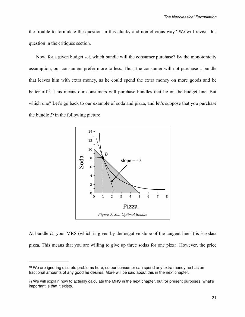
Now, for a given budget set, which bundle will the consumer purchase? By the monotonicity

assumption, our consumers prefer more to less. Thus, the consumer will not purchase a bundle

that leaves him with extra money, as he could spend the extra money on more goods and be

better off13. This means our consumers will purchase bundles that lie on the budget line. But

which one? Let’s go back to our example of soda and pizza, and let’s suppose that you purchase

the bundle D in the following picture:

80 1 2 3 4 5 6 7

14

0

2

4

6

8

10

12

Pizza

Soda

Dslope = - 3

Figure 5: Sub-Optimal Bundle

At bundle D, your MRS (which is given by the negative slope of the tangent line14) is 3 sodas/

pizza. This means that you are willing to give up three sodas for one pizza. However, the price


21

13 We are ignoring discrete problems here, so our consumer can spend any extra money he has on fractional amounts of any good he desires. More will be said about this in the next chapter.

14 We will explain how to actually calculate the MRS in the next chapter, but for present purposes, whatʼs important is that it exists.

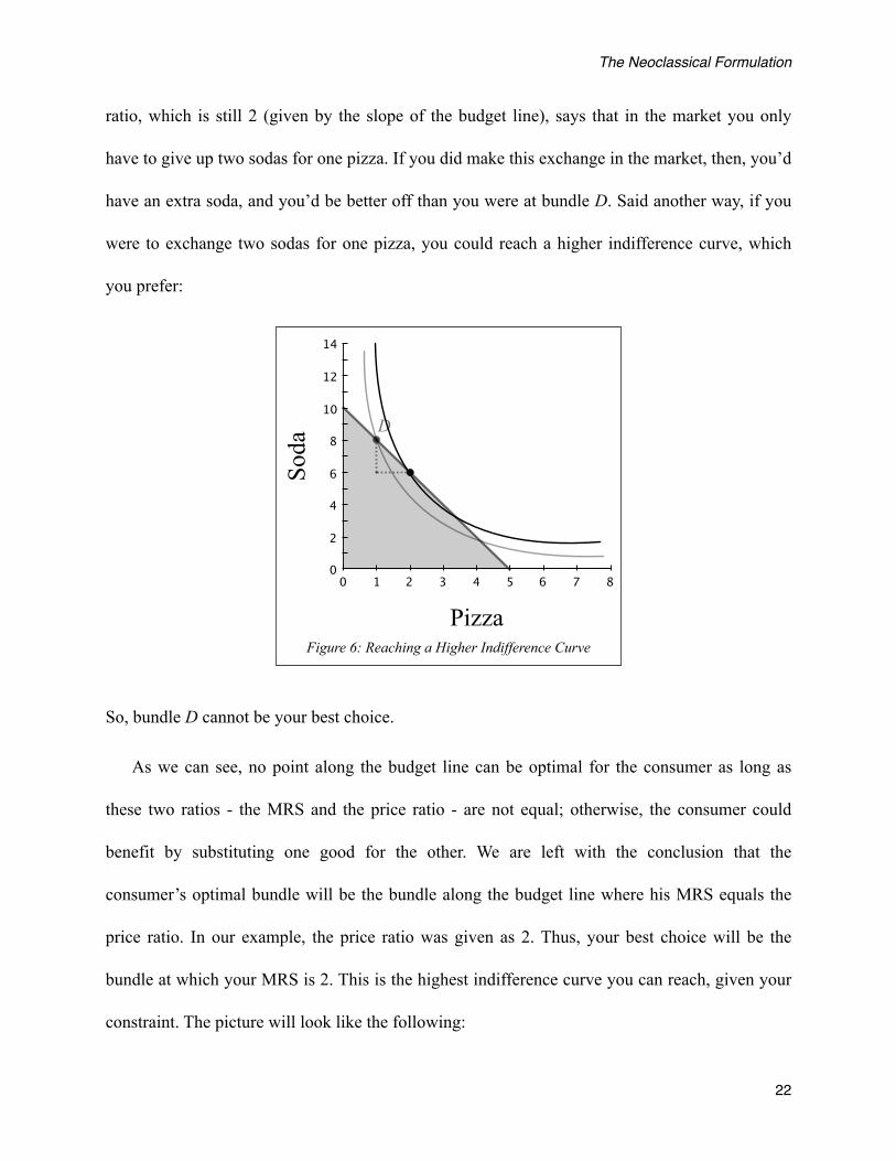
ratio, which is still 2 (given by the slope of the budget line), says that in the market you only

have to give up two sodas for one pizza. If you did make this exchange in the market, then, you’d

have an extra soda, and you’d be better off than you were at bundle D. Said another way, if you

were to exchange two sodas for one pizza, you could reach a higher indifference curve, which

you prefer:

80 1 2 3 4 5 6 7

14

0

2

4

6

8

10

12

Pizza

Soda

D

Figure 6: Reaching a Higher Indifference Curve

So, bundle D cannot be your best choice.

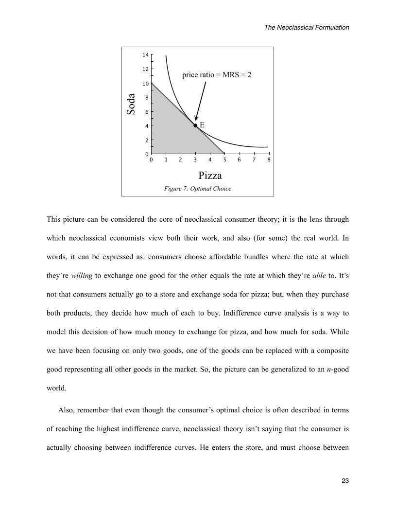
As we can see, no point along the budget line can be optimal for the consumer as long as

these two ratios - the MRS and the price ratio - are not equal; otherwise, the consumer could

benefit by substituting one good for the other. We are left with the conclusion that the

consumer’s optimal bundle will be the bundle along the budget line where his MRS equals the

price ratio. In our example, the price ratio was given as 2. Thus, your best choice will be the

bundle at which your MRS is 2. This is the highest indifference curve you can reach, given your

constraint. The picture will look like the following:


22

80 1 2 3 4 5 6 7

14

0

2

4

6

8

10

12

Pizza

Soda

price ratio = MRS = 2

E

Figure 7: Optimal Choice

This picture can be considered the core of neoclassical consumer theory; it is the lens through

which neoclassical economists view both their work, and also (for some) the real world. In

words, it can be expressed as: consumers choose affordable bundles where the rate at which

they’re willing to exchange one good for the other equals the rate at which they’re able to. It’s

not that consumers actually go to a store and exchange soda for pizza; but, when they purchase

both products, they decide how much of each to buy. Indifference curve analysis is a way to

model this decision of how much money to exchange for pizza, and how much for soda. While

we have been focusing on only two goods, one of the goods can be replaced with a composite

good representing all other goods in the market. So, the picture can be generalized to an n-good

world.

Also, remember that even though the consumer’s optimal choice is often described in terms

of reaching the highest indifference curve, neoclassical theory isn’t saying that the consumer is

actually choosing between indifference curves. He enters the store, and must choose between


23

bundles in his affordable set. His preference relation tells him that for each pair of bundles, either

he likes one better than the other, or else has no preference between them at all. So, given his

preference relation, he will be able to ordinally rank all the bundles in his affordable set. Since

his indifference curves are assumed to be smooth (by convexity), there will be a single, unique

bundle which is ranked 1st on his list. This is the bundle he will choose, and at this bundle, the

MRS will equal the price ratio.

Indifference curve analysis is viewed very differently by economists, which is one of the

reasons evaluating it is so difficult. For now, we simply want to stress that, whatever it’s purpose,

the picture in Figure 7 above comes exclusively from the consumer’s underlying preference

relation, and the exogenously given prices and income. We will soon see how mainstream

economics transforms the consumer’s choice problem into one of mathematical maximization via

the use of utility functions; but this doesn’t change our analysis. The consumer’s optimal bundle

is still found from the parameters of his problem and his preference relation alone.

1.5 Consumer Demand

Now that we have seen which bundle of goods our consumer will choose for a given array of

market prices, we can construct his demand curves for the various goods. A demand curve is a

locus of points which summarizes how many units of a good a consumer would buy at various

prices. Deriving the demand curve is a straight-forward process, given our analysis of consumer

choice.


24

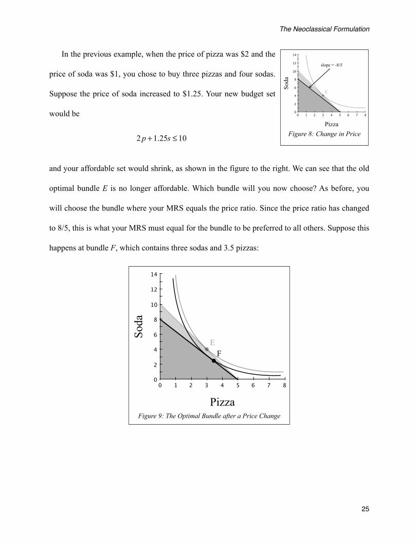
In the previous example, when the price of pizza was $2 and the

price of soda was $1, you chose to buy three pizzas and four sodas.

Suppose the price of soda increased to $1.25. Your new budget set

would be

2 p +1.25s ≤ 10

and your affordable set would shrink, as shown in the figure to the right. We can see that the old

optimal bundle E is no longer affordable. Which bundle will you now choose? As before, you

will choose the bundle where your MRS equals the price ratio. Since the price ratio has changed

to 8/5, this is what your MRS must equal for the bundle to be preferred to all others. Suppose this

happens at bundle F, which contains three sodas and 3.5 pizzas:

80 1 2 3 4 5 6 7

14

0

2

4

6

8

10

12

Pizza

Soda

EF

Figure 9: The Optimal Bundle after a Price Change

80 1 2 3 4 5 6 7

14

0

2

4

6

8

10

12

Pizza

Soda

slope = -8/5

E

Figure 8: Change in Price


25

The increase in the price of soda has thus caused you to decrease your consumption of soda and

increase your consumption of pizza, as we would expect15.

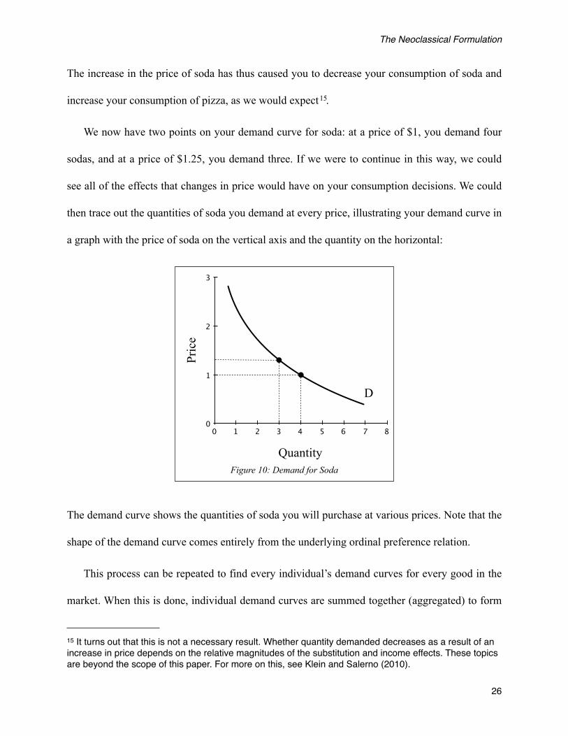
We now have two points on your demand curve for soda: at a price of $1, you demand four

sodas, and at a price of $1.25, you demand three. If we were to continue in this way, we could

see all of the effects that changes in price would have on your consumption decisions. We could

then trace out the quantities of soda you demand at every price, illustrating your demand curve in

a graph with the price of soda on the vertical axis and the quantity on the horizontal:

80 1 2 3 4 5 6 7

3

0

1

2

Quantity

Price

D

Figure 10: Demand for Soda

The demand curve shows the quantities of soda you will purchase at various prices. Note that the

shape of the demand curve comes entirely from the underlying ordinal preference relation.

This process can be repeated to find every individual’s demand curves for every good in the

market. When this is done, individual demand curves are summed together (aggregated) to form


26

15 It turns out that this is not a necessary result. Whether quantity demanded decreases as a result of an increase in price depends on the relative magnitudes of the substitution and income effects. These topics are beyond the scope of this paper. For more on this, see Klein and Salerno (2010).

the market (aggregate) demand curve for each good. These market demand curves are combined

with the familiar market supply curves to arrive at an equilibrium price, which is simply the price

at which quantity demanded equals quantity supplied. Thus, starting with the key axiom of

neoclassical consumer theory - the preference relation - we have derived a result for the quantity

and price of each good in the economy in equilibrium. This is the primary output of consumer

theory, the solution set to the problem of individuals, each optimizing, and each exchanging with

one another in a society.


27

2 Utility FunctionsThe development of consumer choice and market demand in this paper has been atypical.

Usually after the consumer’s preference relation is defined, a mathematical function is

introduced which is said to represent the preference relation. By this, the textbooks mean that the

function contains all of the relevant information about the consumer’s underlying preference

relation, namely, whether or not one bundle is preferred to another, and what the MRS is at

various bundles. These two properties are what define a consumer and his choice decisions in the

market. Since the function reproduces these properties, the consumer’s choice problem becomes

one of mathematical optimization.

The reason this paper has been organized differently is because these representative functions

have been the target of many Austrian critiques. In fact, as this paper has shown, the

representative function should not be considered a core part of neoclassical theory. The

neoclassical theory of consumer choice is: given a consumer’s preferences, how does he decide

how much of which goods to buy in the market? All that is necessary to answer this question is

(1) the graph of his indifference sets and budget line, and (2) the existence of a line that’s tangent

to the indifference set and whose slope (MRS) is equal to the slope of the budget line. The

indifference set and MRS come from his preference relation. Thus, any properties of the

representative function which go beyond these two are irrelevant for the analysis, and should be

treated as such.

2.1 Utility Functions and the Representation Theorem

28

We will now see how neoclassical economics converts the consumer’s choice problem as

presented above into one of mathematical optimization. First, we introduce the utility function:

Utility Function

A utility function is a mathematical representation of the consumer’s preferences . The

utility function u : X → assigns a numerical value to each bundle of goods in the set X

according to the following rule:

x y iff u(x) ≥ u( y)

and

x y iff u x( ) > u y( )

Such a utility function is said to represent the consumer’s preferences .

So the domain of the function is bundles of goods, and the range is the set of real numbers i.e.

pure numbers that have no units16. Since elements in X are of the same topological structure (i.e.

each bundle is a k-tuple), the function u is well-defined. But given the consumer’s preferences,

does such a function even exist? It turns out that if we assume rationality and continuity, our

consumer’s preferences will always be representable by a utility function17. The theorem which

Utility Functions

29

16 Sometimes, the range of the utility function is has an arbitrary, meaningless unit, such as a util, although this has caused much confusion on the topic of cardinal utility. This will be elaborated upon shortly.

17 Other versions of the representation theorem include different assumptions, such as reflexivity or some form of monotonicity. Cf. Varian (1992, p. 97) and Mas-Collel (1995, p. 47).

proves the existence of the utility function is called the representation theorem. Its proof has

been omitted18.

Let’s look at an example of a utility function, considering only two goods, x and y. Suppose a

consumer has rational, continuous preferences which rank different goods, and suppose the

representative utility function (the function which represents his preferences) is

u x, y( ) = xy

Now, suppose we have the bundle (2, 3), which is the bundle containing two units of good x and

three units of good y. Then, the function would assign the number 6 to the bundle, since

u 2,3( ) = 2 ⋅3 = 6

Again, the range of the utility function is the set of real numbers, so the number 6 to which the

utility function assigns the bundle (2, 3) is a pure number; it has no units. For this reason, the

number 6 itself is meaningless. As the definition of the utility function indicates, the utility

function compares bundles - just as the preference relation does. Thus, we can take another

bundle, say (1, 4), and see how it compares to the first:

u 1,4( ) = 1⋅4 = 4

Since 6 is greater than 4, this means that the bundle (2,3) is preferred by the consumer to the

bundle (1,4); that is,

2,3( ) 1,4( )

Utility Functions

30

18 For those interested, see Mas-Collel, pg. 47.

Now, how does the utility function reproduce indifference? From our definition of

preferences, we know that a consumer will be indifferent between two bundles (x1, y1) and (x2,

y2) if both

x1, y1( ) x2 , y2( ) and

x2 , y2( ) x1, y1( )

By the definition of the utility function, this will be true if both

u x1, y1( ) ≥ u x2 , y2( ) and

u x2 , y2( ) ≥ u x1, y1( )

which implies that

u x1, y1( ) = u x2 , y2( )

Thus, consider the bundles (2, 4) and (1, 8) with the specific utility function described above.

Since

u 2,4( ) = 2 ⋅4 = 8

and

u 1,8( ) = 1⋅8 = 8

the consumer is indifferent between the two bundles; that is,

2,4( ) ~ 1,8( )

So, the utility representation tells us whether the consumer prefers one bundle of goods to the

other, or whether he is indifferent between the two. Even so, remember that these orderings are a

Utility Functions

31

property of the underlying preference relation, and that the utility function is merely reproducing

them.

The utility function can also reproduce the MRS, which is the second important property of

the preference relation. To see this, we want to be able to graph our indifference sets, just as we

did when we first introduced the MRS. So, how can we graph indifference sets using only our

utility function?

As was just explained, the consumer is indifferent between two bundles if the utility function

assigns those two bundles the same real number. This means that an indifference set is simply the

set of all bundles which are assigned the same number by the utility function. Recall that an

indifference set is defined in terms of a certain bundle (x*, y*). Suppose our utility function

assigns to this bundle the real number 4. Then, the indifference set containing the bundle (x*, y*)

is the set of all bundles which are assigned the number 4 by the utility function; that is,

x, y( ) : u x, y( ) = xy = 4{ }

Again, the number 4 itself has no relevance except insofar as it is used to identify which bundles

the consumer finds indifferent to the bundle (x*, y*). It does not refer to anything real or tangible,

or to any part of the consumer’s preference relation.

The reader may already have recognized that the above definition of the indifference set

resembles the mathematical concept of a level set. The level set of a function is the set of all

points for which a function returns a certain constant. Thus, indifference sets can be found by

finding the level sets of the utility function. This is an extremely convenient way to find and

graph indifference sets. However, one must not let this alter one’s perception of what an

Utility Functions

32

indifference set is. An indifference set is not, by definition, the level set of a function; rather, an

indifference set is a set of bundles between which the consumer has no preference. It just turns

out that the indifference set can be found by finding the level set of the representative utility

function. This distinction is important.

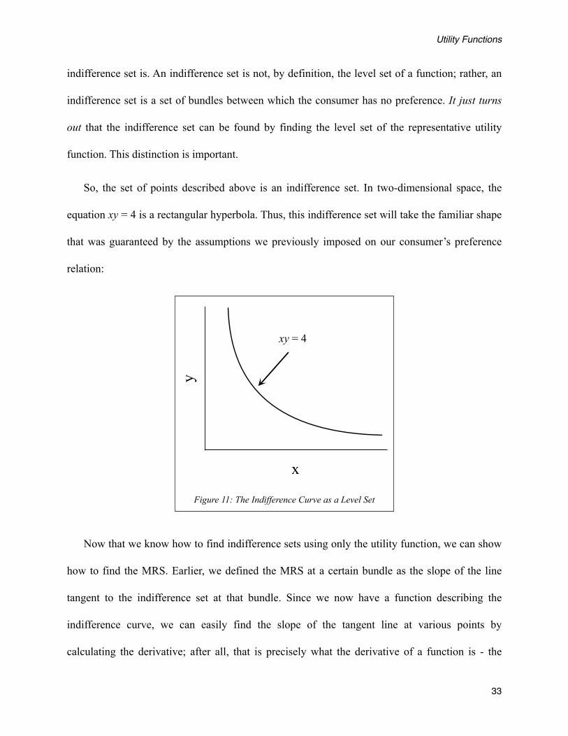
So, the set of points described above is an indifference set. In two-dimensional space, the

equation xy = 4 is a rectangular hyperbola. Thus, this indifference set will take the familiar shape

that was guaranteed by the assumptions we previously imposed on our consumer’s preference

relation:

x

y

xy = 4

Figure 11: The Indifference Curve as a Level Set

Now that we know how to find indifference sets using only the utility function, we can show

how to find the MRS. Earlier, we defined the MRS at a certain bundle as the slope of the line

tangent to the indifference set at that bundle. Since we now have a function describing the

indifference curve, we can easily find the slope of the tangent line at various points by

calculating the derivative; after all, that is precisely what the derivative of a function is - the

Utility Functions

33

slope of the tangent. Note that we’re interested in the derivative of the indifference curve (i.e. the

level set), not the derivative of the utility function.

Since our indifference curves (level sets) are expressed in terms of both goods x and y (that

is, since the level sets are implicit functions of the two goods, rather than being explicit functions

of either good individually), we cannot calculate its derivative directly. Instead of rearranging the

indifference curve in terms of one variable and then calculating the derivative, neoclassical

economists conventionally employ the implicit function theorem19, which states that a derivative

dy/dx can be found given an implicit function f of both variables via the following formula:

dydx

= −∂f / ∂x∂f / ∂y

Thus, given an implicit function of x and y, the negative ratio of the partial derivatives will give

us the slope of the tangent line (i.e. the derivative) of the indifference curve. In our case, the

utility function is an implicit function of both goods (u is a function of x and y), so the derivative

of the indifference curve will be the ratio of the partial derivatives of the utility function:

slope of tangent of indifference curve = −

∂u / ∂x∂u / ∂y

Finally, since the MRS is the negative of the slope of the tangent line, we are left with

MRS = −slope of tangent =

∂u / ∂x∂u / ∂y

Utility Functions

34

19 For more details, see http://en.wikipedia.org/wiki/Implicit_function_theorem.

http://en.wikipedia.org/wiki/Implicit_function_theorem

http://en.wikipedia.org/wiki/Implicit_function_theorem

This is how we find the MRS using only the utility function. Just as we stressed when we

explained that indifference sets can be found by looking at the level sets of the utility function,

the fact that the MRS is the ratio of derivatives of the utility function shouldn’t affect how we

think of the MRS. The MRS is the rate at which a consumer is willing to exchange one good for

another on the margin, and it exists even if we never introduce utility functions. It just turns out

that the MRS will equal the ratio of derivatives of the utility function.

Note the units of the numerator and denominator of this representation of the MRS. The

utility function returns a pure number; however, when we take the partial derivative, we are

dealing with a rate of change, just as we do whenever we take a derivative. It becomes how fast

this pure number is changing for tiny changes in either good. Thus, the units of ∂u / ∂x are “per

x.”20 Similarly, the denominator is in units of “per y.” Then, the slope will be in units of “per x /

per y,” or, more simply, in “y per x.” This unit is equivalent to the slope of the tangent that we

found in the previous chapter, as well as the units of the price ratio.

Now that we know how to find the MRS using the utility function, our description of

consumer choice proceeds exactly as in Section 2.3 above. The most preferred bundle the

consumer can afford is found by choosing the bundle on the budget line where the MRS equals

the price ratio. In terms of the utility function, it’s where

∂u / ∂x∂u / ∂y

=px

py

Utility Functions

35

20 If an arbitrary unit has been assigned to the utility function, the units of the derivative would be “utils per x.”

In our example, with a utility function of u = xy, the MRS is

MRS =

∂u / ∂x∂u / ∂y

=yx

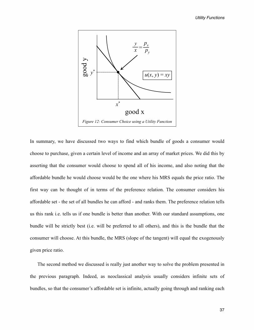
which we can see clearly depends on how much x and how much y the consumer has. If we were

given the prices the consumer faces and the income he has, we could use that information to find

the consumer’s optimal bundle. The first equation ensures the slope of the consumer’s

indifference curve will equal the slope of the budget line

MRS =

yx=

px

py

and the second ensures the bundle will be on the budget line:

px x + py y = I

These two equations can be solved to find the bundle (x*, y*) which would be the consumer’s

optimal choice.

Utility Functions

36

good x

good

y

yx py

px=

x*

y* u(x, y) = xy

Figure 12: Consumer Choice using a Utility Function

In summary, we have discussed two ways to find which bundle of goods a consumer would

choose to purchase, given a certain level of income and an array of market prices. We did this by

asserting that the consumer would choose to spend all of his income, and also noting that the

affordable bundle he would choose would be the one where his MRS equals the price ratio. The

first way can be thought of in terms of the preference relation. The consumer considers his

affordable set - the set of all bundles he can afford - and ranks them. The preference relation tells

us this rank i.e. tells us if one bundle is better than another. With our standard assumptions, one

bundle will be strictly best (i.e. will be preferred to all others), and this is the bundle that the

consumer will choose. At this bundle, the MRS (slope of the tangent) will equal the exogenously

given price ratio.

The second method we discussed is really just another way to solve the problem presented in

the previous paragraph. Indeed, as neoclassical analysis usually considers infinite sets of

bundles, so that the consumer’s affordable set is infinite, actually going through and ranking each

Utility Functions

37

of the bundles could potentially be an impossible job. Thus, we invoke the utility function to

‘streamline’ this process. The level set of the utility function gives us the consumer’s indifference

sets. The derivative of this level set, which is given by the ratio of the derivatives of the utility

function, gives us the MRS. When this equals the price ratio, the consumer cannot benefit from

substituting, and assuming he is choosing a bundle on his budget line, he is spending all of his

money. Thus, we will find the same bundle that we did using the first method. The utility

function, while making the process of finding the optimal bundle easier, has not at all changed

the fundamental nature of the consumer’s choice problem.

2.2 The Utility Maximization Problem

The second method we just described for finding the consumer’s optimal bundle is often

framed in terms of a maximization problem. In the language of constrained optimization, the

consumer wants to maximize his utility function, choosing x and y, subject to his budget

constraint:

Maxx , y u x, y( )s.t. px x + py y = I

Such a constrained maximization problem is generally solved using the method of Lagrangian

multipliers. The solution will yield us back the same two conditions which characterize our

original solution, namely, one saying the MRS will equal the price ratio, and one saying the

bundle will be on the consumer’s budget line.

Utility Functions

38

Thus, we see that calling the problem a “utility maximization” problem changes absolutely

nothing. The consumer’s choice problem is fundamentally the same. The relevant piece of

information we obtain via the utility function - the MRS - is an aspect of the preference relation,

just as it always was. Just because we are maximizing a utility function, doesn’t mean we now

conceive of ‘utility’ as some quantity, measurable or otherwise. In fact, the term ‘utility’ should

probably not be used at all, since it is so easily confused with the cardinal utility functions that

were once part of mainstream economics. The function could simply be called a “ranking

function” which the consumer wants to maximize i.e. he wants to choose that affordable bundle

which obtains the highest rank based on his preferences.

2.3 Marginal Utility

The partial derivatives of the utility function are often called the marginal utilities of the

goods in question. For example, the partial derivative of the utility function u with respect to the

good x would be called the marginal utility of good x:

∂u∂x

= MUX

Using this notation, the MRS is often written as the ratio of marginal utilities:

MRSYX =MUX

MUY

This terminology has been explicitly left out of the above discussion as it, like the term utility

function, is likely to cause confusion. Since the first derivative of the utility function has no

Utility Functions

39

relation to anything from the preference relation, it has no economic meaning. It simply is what it

is: a mathematical derivative. Just as with the numbers to which the utility function assigns

bundles, the marginal utilities have no intrinsic meaning.

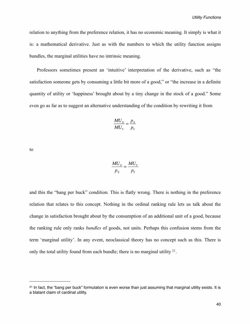
Professors sometimes present an ‘intuitive’ interpretation of the derivative, such as “the

satisfaction someone gets by consuming a little bit more of a good,” or “the increase in a definite

quantity of utility or ‘happiness’ brought about by a tiny change in the stock of a good.” Some

even go as far as to suggest an alternative understanding of the condition by rewriting it from

MUX

MUY

= pXpY

to

MUX

pX= MUY

pY

and this the “bang per buck” condition. This is flatly wrong. There is nothing in the preference

relation that relates to this concept. Nothing in the ordinal ranking rule lets us talk about the

change in satisfaction brought about by the consumption of an additional unit of a good, because

the ranking rule only ranks bundles of goods, not units. Perhaps this confusion stems from the

term ‘marginal utility’. In any event, neoclassical theory has no concept such as this. There is

only the total utility found from each bundle; there is no marginal utility 21.

Utility Functions

40

21 In fact, the “bang per buck” formulation is even worse than just assuming that marginal utility exists. It is a blatant claim of cardinal utility.

As a clarifying point, Austrians mean something entirely different by the term marginal

utility than neoclassicals do. For an Austrian, the marginal utility of a good is defined as the

satisfaction brought about by the least-valued end among all ends which a stock of homogenous

goods is serving. The word ‘marginal’ applies to a definite, discrete unit of a good (namely, that

good which is being applied to the least-valued end); and the term ‘utility’ refers to the

satisfaction brought about by the achievement of the least-valued end. In contrast, when a

neoclassical uses the term marginal utility, he means the derivative of the utility function with

respect to a certain good. That is all he means; or, rather, that is all he should mean.

2.4 Uniqueness, Ordinality and Cardinality

What’s important about the utility function? One, its ability to reproduce the ordering of

bundles; and two, its ability to reproduce the MRS.

When we first introduced utility functions, it was via the representation theorem. The

theorem stated that if a certain preference relation satisfied the assumptions of rationality and

continuity, then a utility representation existed. Note that the theorem said nothing about

uniqueness. It is therefore natural to ask if such a representative utility function is, in fact,

unique, or if there are many utility functions which can all ‘represent’ the same preference

relation. As one of the main properties of the utility function is its ability to order bundles i.e. to

compare one bundle to another, it would seem likely that a given utility representation would not

be unique. It turns out that this is the case. In fact, our intuition carries through quite nicely on

this point. We know that if we start out with a utility function which represents a certain

preference relation, that utility function will rank one bundle higher than another whenever the

Utility Functions

41

underlying preference relation does so. It does this by assigning a higher real number to the

preferred bundle. Since the only thing we do with these real numbers is compare them, all that’s

important for the utility function to produce the same ranking is that the relative positions of the

real numbers assigned to the bundles remain unchanged. Thus, any transformation applied to the

utility function which doesn’t alter the ordering of the bundles will represent the original

preference relation in precisely the same way as the first utility function did. In this sense - and

in only this sense - utility functions are said to be ordinal in character.

Now, of course, the utility function itself is a cardinal function. This is true simply because

its range is the set of real numbers, which are cardinal numbers (e.g. 2, 5.43, …) rather than

ordinal numbers (1st, 5th, ...); but it does not follow from this that neoclassical economics

conceives of utility as a cardinal quantity22. The cardinal numbers themselves have no economic

meaning; they don’t relate in any way to the preference relation. Only the relation between the

numbers is important, just as the relation between two bundles is important for the preference

relation.

Being a mathematical function, the utility function of course has many additional properties

besides the two that have been stressed in this paper. For example, its arguments can be added,

subtracted, multiplied, etc. However, none of these properties matter. The sole purpose of the

utility function, as far as consumer theory goes, is to find the tangent line to an indifference

curve. This is done by the process explained above. Any additional properties the utility function

Utility Functions

42

22 Before the work of Carl Menger, Daniel Bernoulli, Jeremy Bentham, Alfred Marshall and others explicitly claimed that utility was cardinal in nature. For more on this, see http://en.wikipedia.org/wiki/Cardinal_utility.

http://en.wikipedia.org/wiki/Cardinal_utility




has are (should be) ignored, and the mere existence of these properties in no way ‘proves’ that

neoclassical economics really conceives of utility in a cardinal manner.

Now, it must be pointed out that the utility function only exists in the first place precisely

because the preference relation was developed in such a way as to make it so. All one needs to do

is look at Figure 7 above to see that an indifference curve so constructed will be the level set of a

mathematical function. But the utility number itself, or any other mathematical properties of the

function (cardinal or otherwise) are not important, and should not be held against the

neoclassical analysis. Critiques that accuse indifference curve analysis of comparing the amount

of utils different bundles offer the consumer are unfounded. The utility function is simply not the

right focus, as the indifference set fundamentally has nothing to do with it. Once the picture in

Figure 7 has been justified, the mathematical representation that follows is logically airtight. The

skeptic of neoclassical economics, then, should critique the assumptions necessary to get to

Figure 7, rather than focus on the representation theorems, or the allegedly cardinal nature of the

utility function23.

Utility Functions

43

23 There are instances in mainstream analysis outside of standard consumer theory that make explicit use of cardinal utility (e.g. Harsanyiʼs model of social choice). In fact, the important field of welfare economics has never fully recovered from the demise of cardinal utility. For more on this, see Herbener (1997).

3 CritiquesThe previous two chapters have outlined the basics of neoclassical consumer theory. Many

parts of the theory have been misunderstood or distorted, and we hope our exposition will

prevent future mistakes of a similar kind. The reader may now have the impression that because

we think many of the alleged faults of neoclassical economics are misunderstandings, we

sympathize with the neoclassical method. In fact, nothing could be further from the truth. The

very existence of these misunderstandings is a testament to the convoluted way of thinking that

is so characteristic of neoclassical economics.

Indeed, these misunderstandings are not limited to those thinkers who have explicitly

critiqued neoclassical thought, such as the Austrians. We would wager that precisely because of

the way neoclassical economics is taught, most students probably unwittingly believe many of

these errors as well. Typically, once the representation theorem is explained in a principles class,

teachers present swaths of problems without ever referencing the preference relation. Exclusive

attention is given to various forms of utility functions, and students become adept at setting up

and solving constrained optimization problems. It is not rare to hear students jokingly ask each

other if they have been maximizing their utility functions that day, or, more disturbingly, to hear

professors cogitate on whether or not such functions actually exist inside of our minds.

In any case, in spite of the alleged faults of neoclassical theory that the first two chapters of

this paper were intended to clear up, plenty of faults remain. The point of this paper is not to

vindicate the neoclassical position, but to aid in our understanding of it so that any critique we

advance is a proper one. To this end, we now describe several major faults of the neoclassical

position on consumer theory.

44

3.1 On Preferences

The science of economics deals with real-world facts, such as market prices, interest rates,

and the production of goods. This seemingly mundane claim carries many profound implications,

an important one being that because these facts exist in the real world, they must have been

caused by real-world events. The concrete, objective nature of an economic fact cannot be

affected by a subjective feeling, thought or intention; people cannot simply will market prices to

fall, nor can they just imagine manufacturing plants into existence. Action, not volition, is what

characterizes social interaction, and this truth is key to understanding what really causes the

economic facts we see around us. Thus, people affect market prices through actually buying or

not buying a good, rather than just thinking about it; and entrepreneurs create manufacturing

plants by actually hiring labor and purchasing raw materials. While none of this seems

disagreeable, there is a subtle yet important corollary to this that is often misunderstood.

In its explanation of economic data, and of the actions by which these data are caused,

economic science inevitably refers back to the human mind. This is appropriate, as a man’s mind

is ultimately responsible for his choosing one action over another (economics tends to set aside

philosophic questions regarding whether man has the capacity for free choice; indeed, were it not

the case, economics itself would cease to exist). This does not imply that it is the task of

economics to explore all the depths of the human psyche. In fact, the discussion above provides a

perfectly natural choice set of which aspects of the human mind are appropriate for economics to

consider: namely, those aspects which cause men to act. In other words, since the science of

economics is concerned with the explanation of real-world facts, and since these facts are caused

Critiques

45

solely by real-world action, the human mind is relevant to economics only insofar as it helps to

explain human action.

The failure of the neoclassical school to apprehend this truth is largely responsible for many

of their misunderstandings. For example, their notion of a preference relation does not describe

human action, but instead attempts to describe human psychology. The preference relation

discussed in the initial two sections of this paper first assumes that some specification of an

individual’s psychological feelings exists, and only then does it analyze the implications of

this specification on his actual decision-making behavior. By taking thought as its starting point

rather than action, the preference relation concerns itself with categories of the human mind that

are irrelevant to economic science. For instance, under the assumptions of the standard

neoclassical preference relation, a consumer is assumed to have feelings about goods which he

could never possibly afford (say a 747 Boeing jet) or which he would never even consider

purchasing (some inexpensive but complicated piece of computer equipment). Since the vast

majority of these feelings have no bearing on which course of action he chooses, they are, by

implication, irrelevant for explaining economic facts, and should not be included in the study of

pure economics. Moreover, these assertions distract the economist in his development of

economic theory as he devotes much time and energy to thinking about and testing them.

A neoclassical economist may contend that feelings which don’t manifest themselves in

action are still important, as they help to explain why we do choose the things we do; yet this

argument misses an important distinction. There is a difference between feelings that are

associated with action, and feelings that are divorced from action entirely. It is perfectly

reasonable to make sense of a boy’s decision to buy chocolate ice cream by considering his

Critiques

46

subjective feelings and values about chocolate ice cream versus vanilla ice cream. But the

preference relation underpinning neoclassical theory describes feelings which are divorced from

action - feelings which simply exist in our minds, at any given moment. Some of these feelings

cause us to act, and some of them don’t, but only the former are important for describing

economic facts. By ignoring this distinction, neoclassical economics attempts to explain

consumer behavior using concepts which perhaps more appropriately belong to the field of

psychology.

Even if we were to accept the neoclassical foundation, though, it is not entirely clear which

thoughts or feelings constitute an actor’s preferences. Let’s say John is at an ice cream shop, and

he is choosing to buy either a vanilla ice cream cone or a chocolate ice cream cone. Suppose

John thinks - or says out loud - that he prefers the vanilla cone to the chocolate cone, but that he

actually ends up buying the chocolate cone. In this case, what would we say John’s preference is

between vanilla and chocolate ice cream?

If we say that John prefers chocolate to vanilla, then not everything he says or thinks can be

regarded as his preferences. But which thoughts and utterances are included in the domain of

preferences, and which are omitted? This question seems an impossible one to answer. The

answer cannot be, “only include those thoughts and utterances which coincide with the

consumer’s actions,” since we already know that consumers have preferences apart from their

actions. Are our ‘true’ preferences deep down inside of us somewhere, not always accessible to

our conscious and potentially in conflict with our thoughts and our words? If this is the

neoclassical position, it is never discussed or justified by professors or textbooks, let alone

established by any of the axioms of consumer theory.

Critiques

47

Now, if we instead claim that John prefers vanilla to chocolate, even though he bought the

chocolate cone, then we are saying that people can act at variance with their own preferences. In

this case, preferences do not explain, or do not completely explain, individual decisions. What is

being left out, and why? John’s decision to purchase chocolate ice cream certainly affects the ice

cream shop’s inventory and its future production decisions; yet nothing in John’s decision, a

decision which affects multiple economic phenomena, can be traced back to his preferences. If

something besides preferences influence individual decision-making, why is the preference

relation the bedrock concept of consumer theory? And whether or not people can act at variance

with their own preferences, the original question is still begging for an answer: what are John’s

preferences?

In Austrian economics, preference relates to action in the following strict sense: every action

establishes a preference for the thing chosen over the things not chosen. Preference is the value

judgement that our mind makes when deciding to choose one course of action over another. If

John buys chocolate ice cream, then, we say that at that moment, he preferred buying chocolate

ice cream to vanilla, or strawberry, or any other flavor. No thoughts or feelings John may have

had could affect our deduction of his preference for chocolate ice cream, since that preference is

exclusively based on his action. As economics is concerned with the explanation of real-world

phenomena, we see that Austrian economics has made a useful distinction between what is

relevant for economic science, and what is not. Since preferences are bound up in action i.e.

since they do not exist independently from human activity, the Austrian analysis of the consumer

is focused on the set of all human actions, which are the only possible explanatory causes of any

economic fact.

Critiques

48

It’s important to note that in Austrian economics, the term preference does not mean the same

thing that it does in everyday parlance. For instance, if a boy says he really prefers going to a

sports game to watching ballet, but he ends up watching ballet anyway to satisfy his girlfriend’s

wishes, an Austrian would still say that the boy prefers watching ballet to going to the sports

game. This poses no serious problem for Austrian economics, though, and indeed we often see

this occurring in other sciences. In physics, the term work means something very specific,

namely: force times distance. A man holding a large rock above his head is therefore doing no

work according to a physicist, even though the man himself would say otherwise. Similarly, the

boy going to the ballet has no preference for going to the sports game according to an Austrian

economist, even though he himself might disagree. When deciding to use certain terms within

fields of knowledge, there is always a tradeoff between the confusion caused by these terms’

definitions conflicting with their everyday usage, and the understanding afforded by their

technical precision. Just as physics has evaluated this tradeoff in favor of giving work a very

specific definition, so too has Austrian economics evaluated the same tradeoff in favor of a more

restricted but powerful definition of preference.

It is abundantly clear that the Austrian definition of preference avoids the problems that

plague the neoclassical system. Already we have seen some of these problems: if preferences

determine action, and are thus not thoughts and utterances (which can conflict with our action),

what are they? If preferences simply influence action, what are we omitting? If preferences have

no impact on action, why do we study them at all? On the contrary, preferences within the

Austrian framework both fully explain and can never contradict a particular action, because only

the aspects of that action are considered in the explanation.

Critiques

49

Since the neoclassical preference relation focuses on thought, it has another problem. The

range of human thought is vast and diverse, and not all human thought lends itself to the kind of

analysis neoclassical economics is aiming at. Thus, the preference relation must quite arbitrarily

exclude many categories of human thought from its domain. For instance, a consumer’s

sentiment that he cannot compare apples and laptops, or that he passionately prefers ice cream to

candy, or that has no opinion about a certain good even though he can afford it (say some

complicated piece of technology), or that his choice between two goods depends on what

somebody else thinks, is ignored altogether. Even though people have these types of thoughts,

they are simply deemed irrelevant for explaining consumer behavior. Recent developments in

microeconomic theory consist of including additional feelings in the preference relation, such as

the intensity of preferences; but still, the choice to include some feelings and exclude others

remains as unjustified as the choices made about those included in the bedrock preference

relation discussed in this paper.

Particularly interesting is the decision to include in the preference relation the feeling of

indifference. It is important to understand what neoclassical economics means by indifference.

Indifference does not describe a possible psychological state of mind someone may experience

when they choose to do something. If you wake up one morning and think, “I don’t care which t-

shirt I wear today,” and just grab one, this is not what indifference is describing. Indifference

means that you cannot choose between two courses of action on the basis of utility. If two

bundles are in the same indifference set, a consumer is indifferent or has no preference between

these two bundles, and so he is unable to choose between them purely on considerations of

utility. In this case, then, the consumer is in a state of non-action. By definition, his non-action is

Critiques

50

not affecting economic phenomena. What does economics have to say about this? Economics

attempts to explain real-world human activity and its implications; it does not claim to also

explain the psychological inner workings of the human mind, or how the human psyche

influences action. Said another way, economics analyzes people’s decisions in light of the fact

that they are pursuing certain ends, but it does not determine or attempt to determine the content

of those ends. So it seems that neoclassical economics has stepped outside of its jurisdiction by

founding its discussions of action on hypothetical and unverifiable postulates about states of non-

action.

A neoclassical economist may respond that an indifference set does, in fact, tell us how a

consumer will act, precisely because it tells us when a consumer will not act. By analyzing which

bundles a consumer is indifferent between, the argument goes, we can know that when he is

faced with a choice from among a feasible set of bundles, the consumer will choose a certain

bundle precisely because he is not indifferent between this bundle and some other affordable

bundle. Indifference sets thus tell us about a consumer’s optimal bundle by describing the set of

non-optimal bundles, and the relationships among these bundles.

But in this case, why use the concept of indifference to explain action at all? This argument

essentially boils down to: a consumer chooses his most preferred bundle. Beyond this lies a mass

of claims about the consumer’s psyche regarding counter-factual (and thus non-realized) acts of

choice. How can we possibly verify that second-in-line to the consumer’s choice bundle was an

indifference set that took a certain shape and contained a certain amount of bundles between

which the consumer wouldn’t have been able to choose, had the optimal bundle not been

available? How can we even say, based on his choice action alone, that this is the reason for his

Critiques

51

decision? For this is what the neoclassical analysis is claiming in its discussions of indifference,

and it is a claim that is unsubstantiated. Nothing in a consumer’s choice action can be linked

back to his indifference sets. This fundamental point must not be overlooked.

To expand on this issue, consider standard neoclassical applied work. An economist takes a

model with consumers who have certain utility functions, finds their demand curves, and then

takes these theoretical demand curves to the data to see how well they predict real-world

decisions. Suppose that some economist’s demand curve perfectly matched all the data from the

buying habits of some real-world individual, and that it continued to perfectly match all future

data as it came out. Would it follow from this that the individual actually had the same

indifference curves that were specified in the model? Even if no other preference relation

produced the same demand points that this particular one did, can we say by process of

elimination that he really had those preferences? We can say nothing of the sort. Comparing the

demand curve that results from consumer optimization to real-world data merely establishes (or

attempts to establish) a relationship between how many units of a good someone will buy at

various prices. It has done nothing to establish the content of the consumer’s subjective

psychological feelings. In particular, it has not shown what bundle he would have chosen, had

the optimal bundle not been available; whether or not any of his ‘preferences’ follow any of the

standard assumptions; or whether or not he is indifferent (to the point of non-action) between any

of the other affordable but non-purchased bundles. That a regression with a ‘perfect fit’ fails to

Critiques

52

validate any of neoclassical consumer theory’s core postulates should seriously call into question

the efficacy of this method24.

Finally, we want to make a small point about the bundle formulation itself. In some capacity,

every person is a consumer. We all have introspective knowledge about the decision-making

process that takes place inside of our minds when we (say) enter a grocery store. Walking down

the aisle, not only do we see various different goods, but several units of each of these goods

available for purchase. We think about what we want to purchase, and then decide how many

units of each good we want. Sometimes we only need one unit of a good, such as one box of

cereal; other times, we need several units, like four stick of butter, or two cans of chicken soup.

It seems like framing the consumer’s choice problem in this way - having a consumer choose

how many units of each good he wants to purchase - would be the most natural. Neoclassical

economics rejects this, however, and instead assumes that consumers choose between different

bundles of goods. Why insist on such a strange complication at the very onset of the analysis?

One answer is that it yields a set of bundles that are topologically equivalent, and that this

condition ensures the representative utility function will be well-defined. If consumers in the

neoclassical model simply chose how many bananas they wanted to purchase (as consumers do

in the real world), it would be impossible to represent their preferences as a function, or

equivalently, to graph the domain space of the utility function. So from the very beginning,

neoclassical economics has sacrificed clarity and realism for support of a mathematical

framework. Why else would we want to represent preferences on a graph?

Critiques

53

24 In passing, it is interesting to note that indifference curves did not gain popularity until it was realized that they were useful in constructing utility functions on the basis of ordinal utility. See Herbener (1997, pp. 87-90).

In short, the neoclassical preference relation forms an unsatisfactory basis for explaining the

choices of economic actors. It unnecessarily discusses preferences apart from action and thus

opens the door for contradictions; it does not make clear what even constitutes a consumer’s

preferences; the very framing of the consumer’s problem as a choice between bundles is

tendentious and affects the nature of the analysis; and finally, the speculative concept of

indifference is one that exists solely in the minds of human beings, can never be demonstrated in

the actual choice that a person makes, and is thus particularly unsuited as an explanation for why

a person has chosen one course of action over another.

3.2 On Rationality and Continuity

The cornerstone of neoclassical consumer theory is the preference relation. As we saw above,

once the preference relation is defined, several assumptions are imposed on it. Disregarding the

problems just discussed with the actual preference relation itself, we’d now like to ask whether

or not the assumptions of completeness, transitivity and continuity are reasonable.

The term rationality given to the assumptions of completeness and transitivity is suggestive

of normative sentiment. Is neoclassical economics claiming that reasonable people have

preferences that satisfy these axioms? Once we grasp the nature of the preference relation, we

can easily see that such a claim cannot be true. Human beings make decisions under uncertainty.

They do not require complete or even abundant knowledge about a certain situation in order to

choose one action over another. Reasonable people do not have ‘rational’ preferences for the

same reason that reasonable people cannot see into the future: people are not omniscient, and do

not algorithmically decide when to do one thing and not another. To act reasonably simply means

Critiques

54

to act on good sense, taking account of the available information, but certainly not considering

an exhaustive list of every permutation available. While the neoclassical assumption of

rationality may be an attempt to capture human behavior that is reasonable according to this

definition, it fails, and instead creates an entirely new breed of ‘economic agents’ that scarcely

resemble human beings at all. To see why, let’s consider each of the rationality assumptions in

turn.

It is manifestly obvious that preferences cannot be complete. For preferences to be complete,

the consumer must have knowledge of the potential satisfaction he can derive from every

combination of all the goods he can afford. Who can possibly make this comparison? More

importantly, is this even reasonable as an ideal? Consider again the simple example of shopping

in a grocery store. When we as consumers decide which items to purchase, we never even see or

consider purchasing many items in the store at all, perhaps because they are not relevant to us, or

perhaps because we simply overlook them. In spite of this, we still make purchases week after

week that we do not regret. These market choices demonstrably show that we can adequately

satisfy our wants, even though our preferences are incomplete. Prices still adjust, inventories still

shift, and the profit-and-loss system still operates, even though consumer decisions in the

marketplace are not backed by omniscience.

A neoclassical economist may respond that if we were to simply limit the information set

over which the consumer is choosing, then his preferences would indeed be complete. Thus, if

we assume the consumer is only choosing between two or three bananas, and one or two boxes

of cereal, and so on, and ignore the vast combinations of goods the consumer never even

Critiques

55

considers, then the completeness condition would hold. At this level, though, the assumption of

completeness boils down to a redundant tautology: consumers consider what they consider.

This is just wordplay, however, and it simply ignores the prime motivation behind the

assumption of completeness. The reason preferences are assumed to be complete in the first

place is precisely so that every possible bundle which the consumer can afford can be evaluated

by him. Only then will his representative utility function be able to return a number for any

bundle in his affordable set, and only then will the techniques of differential calculus be available

for finding his optimal bundle. If this were not so, the functional approach would merely become

a clunky way to restate the consumer’s obvious choice problem of deciding how many units of

various goods he wants to purchase.

The assumption of transitivity is likewise imposed to ensure the existence of a utility

function, and it’s easy to see why. Take the just perceptible differences example of room

temperature given in section one of this paper. Clearly, examples such as this abound in our daily

lives, giving us good reason to question the relevance of transitivity. Furthermore, even if we

ignore these problems, there are times when our preferences are simply not transitive. Why can

someone not prefer an apple to a banana, a banana to an orange, and an orange to an apple? The

neoclassical economist may respond that he could never choose between all three, but this would

be an error in reasoning stemming from the nebulous relationship between preferences so

conceived and action. Certainly a man would choose something were he faced with all three;

again, this says nothing about what he would have chosen were he faced with other options.

Nothing is absurd or even odd about this. We can find no intuitive or natural reason why one’s

preferences ought to satisfy the condition of transitivity. So why is transitivity included? It turns

Critiques

56

out that transitivity is a necessary condition for the proof of the representation theorem, since it

guarantees that indifference curves do not cross. This strengthens the inference that the

elementary neoclassical assumptions have been included in the analysis not because of their

economic considerations, but simply because they are necessary building blocks for a

mathematical framework. The question of whether such a framework occupied by economic

agents even applies to a real world populated with flesh-and-blood human beings is often left

unanswered.

Finally, the assumption of the continuity of preferences clearly does not appeal to reality, and

almost no neoclassical economist contends that it does. A good is defined by the human need that

it serves, and goods are the object of consumer demand. This is the basis of consumer theory.

What need is being served by 2.873 laptop computers? Such a unit does not exist, nor is it even

conceivable to the human mind. Human beings make decisions between discrete units of goods,

so the assumption of continuity does not hold for human beings. So why is it included? As was

noted earlier, most mainstream economists probably see continuity as an approximating or

simplifying assumption, one which sacrifices little economic content. But is this true? The

continuity assumption is what paves the way for mathematical conditions characterized by the

equality of economic variables, such as equality of the MRS and the price ratio in consumer

choice. But in the real world, trade is characterized by inequality of value. A consumer buys

successive units of a good until the remaining available units are worth less to him than his

money; and the last unit he bought was worth more to him than the money he paid for it - or else

he would not have bought it. Thus, the assumption of continuity, rather than being innocuous,

Critiques

57

leads economic theory down a path of mathematical deductions whose real-world applicability is

extremely dubious.

Note that even if the assumption led to a model with strong predictive power, the real-world

applicability of the content of the model is never justified (i.e. whether the story the model tells

is what’s really going on), since the continuity assumption is merely asserted from the outset.

Continuity is obviously not a feature of the world we live in, and thus, any implications that

follow from it, while they may apply to a model, do not apply to our reality.

Even if we grant the standard assumptions of rationality and continuity, neoclassical

economics must still admit that it excludes certain individuals from the analysis. The core

textbooks admit this. It seems like neoclassical economics is claiming that consumers with

incomplete or intransitive preferences have little or no effect on market prices, thereby

warranting their omission; yet, such a judgement is not at all being made. The assumptions are

simply necessary conditions for representing the consumer’s preferences in functional form, and

thus they are justified. It is worth noting that Austrian economics does not exclude any individual

from its analysis, as indeed it shouldn’t: a consumer’s purchase of a good affects economic

phenomena, regardless of why the consumer chose to purchase that good in the first place.

3.3 On Convexity

Are preferences convex? There are many cases where it seems like they are. For example,

people generally prefer a diverse arrangement of what they eat or what media they enjoy to just

consuming the same thing over and over again. But the convexity assumption is actually much

Critiques

58

more technical than this, and we will see that its real-world applicability has not been established

by neoclassical theory.

First, it must be pointed out that for preferences to be convex, the underlying set of choice

bundles must also be convex. This means that for any two bundles in the set X, any combination

of the items in these two bundles must also belong to the set X, including fractions of the items.

This condition obviously fails to hold, as we do not see fractions of units of goods in the grocery

store. But let us pass over this problem.

We can think of several occasions where we’d prefer one unit or another, rather than a

mixture of both. As we discussed above, many people would probably prefer a glass of milk or a

glass of orange juice to half a glass of each. Surely we can think of countless other examples

such as this. But might the convexity assumption at least provide some insights about actual

consumer decision-making, even if these insights are only approximations?

As it turns out, the plausibility of convexity is only superficial. The fundamental problem

with the assumption of convexity is that it’s a claim about indifference, and not action.

Convexity describes the shape of an indifference curve. So even if you choose two apples and

two oranges instead of four oranges only, or you take more time off of work as your income

rises, or you spend roughly the same amount of time reading and watching TV during a week

rather than spending all of your time on one activity, or you attempt to spend approximately the

same amount of your income on consumption year after year, your action has done nothing to

establish any claims about the convexity of your preferences. This is a crucial point. It is true that

the assumption of convex preferences implies the types of choice behavior given in the previous

examples; but it does not follow, from that consideration alone, that observing those types of

Critiques

59

behaviors implies that preferences are convex. It is simply a logical fallacy to say that the latter

necessarily follows from the former. Purchasing a diverse bundle of goods merely demonstrates

that you prefer that bundle to all others; it says nothing about the set of bundles that you have not

chosen. It does not specify which bundles you would have been indifferent between, or even if

you would have been indifferent between any two bundles at all; it does not establish that you

would have always or even sometimes preferred a linear combination of any two goods; and it

does not show that the MRS equals the price ratio, or more importantly, that the MRS even

exists.

It is important here to be precise. If preferences are convex (and all the other standard

assumptions hold), it is true that certain things follow: linear combinations of bundles will be

more preferred, the MRS will exist, the optimal choice solution will be unique, and so on. We are

not denying this. However, the question we must ask ourselves is, what evidence do we have for

this assumption of convexity? Does our introspective knowledge about our own preference for

diversity lend support to the hypothesis of convexity? Said another way, if convex preferences

imply diverse decision-making, does the converse hold - namely, does diverse decision-making

imply convex preferences? The answer is that diverse decision-making does not imply convex

preferences, any more than diverse decision-making implies the existence (or non-existence) of

indifference sets. To make this point in the extreme, nothing about a choice for diversity

precludes the possibility that each bundle in the consumer’s affordable set belongs to a separate

indifference set. If the consumer’s choice action doesn’t even imply the existence of indifference

curves, then, how can we possibly say that it implies these curves take a certain shape?

Critiques

60

So we see the fundamental flaw with the assumption of convexity - or more generally, any

assumption that describes the shape of an indifference curve. These assumptions can never be

meaningfully corroborated by any observation or experience. Convexity is a foundational

working assumption in neoclassical economics, yet it remains completely hypothetical and

unverifiable. Indeed, Sir John Richard Hicks, one of the originators of indifference curve

analysis, called the assumption of convexity a “rabbit out of a hat” (Hicks 1975, Chapter I §8 p.

23). Why then is convexity assumed? One answer is that without convexity, the methods of

differential calculus would not be applicable to solving the consumer’s optimization problem.

Convexity sets the stage for calculus because convex preferences guarantee that a solution to the

consumer’s choice problem will exist i.e. that the MRS will exist. Where there’s an MRS,

calculus can be used to find the solution. Without convexity, economists would lose the revered

tools of differential calculus they adopted from the methods of physics.

3.4 On Marginal Utility

The neoclassical conception of preferences is devoid of any proper notion of marginal utility.

In Austrian economics, marginal utility is the satisfaction of the least-valued need that a unit of a

homogenous stock of goods is serving. It follows from this and the principle of economizing that

the marginal utility of any good diminishes as the stock of that good increases. This is known as

the law of diminishing marginal utility.

Marginal utility used to be an important part of mainstream economics, but since the advent

of indifference curve analysis, the economic concepts of marginal utility and diminishing

marginal utility are nowhere to be found. They have been replaced with the assumption of

Critiques

61

diminishing marginal rates of substitution25 (i.e. convexity), which as we know refers to the

slope of an indifference curve.

Neoclassical economists often call the partial derivative of the utility function the marginal

utility of a good; however, since this term doesn’t relate to any part of the preference relation, it

has no economic content whatsoever. Mainstream economic problems will often stipulate a

utility function which exhibits diminishing marginal utility, in the sense that the first partial

derivatives are declining; but again, this doesn’t relate to the consumer’s preferences in any way.

To see this, recall that when we apply positive monotonic transformations to a utility function,

we get a new function that represents the same underlying preference relation. Consider the

following utility function:

u x( ) = ln x( )

Clearly, this utility function exhibits diminishing marginal utility, since its first derivative is

decreasing. Now, if we exponentiate both sides (a positive monotonic operation), we get

v x( ) = eu x( ) = x

This new utility function, which represents the same underlying preferences, no longer displays

diminishing marginal utility. So we see that diminishing marginal utility is simply a property of

Critiques

62

25 As Arrow (1984, p. 41) said,"It may be doubted that this assumption [of diminishing MRS] is really empirically verifiable, and in any case it is an assumption of a totally different logical order from that of utility maximization itself. The older discussions of diminishing marginal utility as arising from the satisfaction of more intense wants first make more sense, although they are bound up with the untenable notion of measurable utility. However, their fundamental point seems well taken."

Of course, marginal utility only implies measurable (cardinal) utility (as Arrow here suggests) if one is devoted to the use of utility functions in economics. In Austrian economics, marginal utility and ordinal utility stand shoulder-to-shoulder, without contradiction.

certain utility functions, and as it’s a property with no connection to the preference relation, it is

of zero economic significance.

In spite of this, neoclassical economists will often loosely talk about marginal utility as if it’s

an economic concept. They will compare first derivatives of different goods and infer that the

economic agent values another unit of the one good more than the other, because one has a

higher marginal utility. This is simply not correct. The concept of marginal utility does not exist

in neoclassical economics. The cardinal numbers yielded by taking the first derivative of the

utility function are just the result of a particular mathematical operation performed on the utility

function; but the primitive economic concept is the preference relation, not the utility function.

The utility function only has meaning insofar as it is able to reproduce characteristics of the

preference relation. As we saw in the exposition above, these characteristics are exclusively two:

the ranking of the goods, and the MRS.

Perhaps the reason this point has been the source of so much confusion is because the

concept of marginal utility is such a natural and intuitive one. It is undeniable that additional

units of a good are less valuable to consumers, since human beings - by the very fact that they act

- apply current goods to their must urgent needs. It follows from this that any additional units of

a good consumers acquire can only be put towards satisfying lower-valued ends. But to be clear,

this concept has been explicitly dropped from the neoclassical analysis, and any reference to it

betrays a false understanding of the theory.

There is yet another way we can see that the concept of marginal utility is inapplicable in

neoclassical analysis. Suppose that which transformations were allowed on the utility function

changed, and that these transformations preserved the original utility function’s property of

Critiques

63

diminishing marginal utility (in the sense of a falling first derivative). Even though diminishing

marginal utility is now preserved, we must remember that what the neoclassical preference

relation ranks is bundles of goods rather than units of goods. Marginal utility is a concept that

requires multiple units of a homogenous good (e.g. bottles of water, horses, cars, etc.). In

neoclassical economics, the consumer never decides between one bottle of water and two; he

decides between a bundle containing one bottle of water and a bundle containing two. Since

every bundle under his consideration is heterogeneous, the economic concepts of marginal utility

and diminishing marginal utility do not apply. So diminishing marginal utility remains an

arbitrary mathematical property of the utility function, rather than a characteristic of the

economic agents of the model.

There is still another misunderstanding about marginal utility that persists in classrooms and

textbooks. Professors may say something along the following lines: when you eat one scoop of

ice cream, you really like it; your second, you like not as much; and your third, even less. Thus,

you have diminishing marginal utility in ice cream, since each scoop provides you with less

satisfaction that the previous scoop. It’s important to understand that reasoning along these lines

is fallacious. Whether the second and third scoops have some undesirable physiological effect

(they make you feel nauseous or give you a headache) has nothing to do with value. Valuation is

a process that takes place inside of our minds, and affects our decisions; it has nothing to do with

physical satiation or regrettable bodily functions. Physiological effects are just facts about action,

whereas value derives from our actual choice action itself.

One last point that is often a source of confusion relates to demand. Demand curves are often

downward-sloping (although within the neoclassical framework they don’t necessarily have to

Critiques

64

be). New students often think that the reason the demand curve is downward-sloping is because

of diminishing marginal utility; that is, the reason I am only willing to buy more units of a good

if the price is lower is because I value those additional units less. While this is true in the

Austrian framework, it is not true in the neoclassical framework. Diminishing marginal utility

doesn’t in any way relate to the demand curve. The shape of the demand curve comes from

assumptions about the shape of the indifference curves i.e. assumptions about the marginal rates

of substitution.

In sum, the concept of utility that results from the neoclassical specification of preferences is

unsatisfactory. In the real world, humans act on the margin. They choose to pursue a certain end,

and in choosing this end, they decide to purchase additional units of a good they evaluate as

serviceable to this end. That is, when acting, humans always consider a little bit more or a little

bit less of a thing. In contrast, economic agents who have the neoclassical preference relation

assign rankings to bundles of all the goods they will potentially consume. Even if we limit the

affordable set to consumption decisions an agent would make in a single trip to the store, the

agent is still assigning total utility to various different combinations of the goods he can afford.

Perhaps the simplest way to sum up the difficulties inherent with the neoclassical conception of

utility is to say that in the real world, there is only marginal utility, and there is no such thing as

total utility; while in neoclassical economics, there is only total utility, and there is no such thing

as marginal utility.

3.5 On Money

Critiques

65

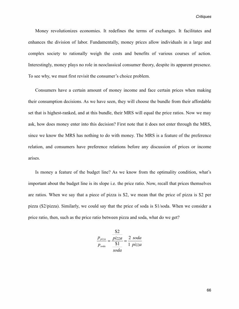
Money revolutionizes economies. It redefines the terms of exchanges. It facilitates and

enhances the division of labor. Fundamentally, money prices allow individuals in a large and

complex society to rationally weigh the costs and benefits of various courses of action.

Interestingly, money plays no role in neoclassical consumer theory, despite its apparent presence.

To see why, we must first revisit the consumer’s choice problem.

Consumers have a certain amount of money income and face certain prices when making

their consumption decisions. As we have seen, they will choose the bundle from their affordable

set that is highest-ranked, and at this bundle, their MRS will equal the price ratios. Now we may

ask, how does money enter into this decision? First note that it does not enter through the MRS,

since we know the MRS has nothing to do with money. The MRS is a feature of the preference

relation, and consumers have preference relations before any discussion of prices or income

arises.

Is money a feature of the budget line? As we know from the optimality condition, what’s

important about the budget line is its slope i.e. the price ratio. Now, recall that prices themselves

are ratios. When we say that a piece of pizza is $2, we mean that the price of pizza is $2 per

pizza ($2/pizza). Similarly, we could say that the price of soda is $1/soda. When we consider a

price ratio, then, such as the price ratio between pizza and soda, what do we get?

ppizzapsoda

=

$2pizza$1soda

=2 soda1 pizza

Critiques

66

So we see that the unit of money (dollars) actually cancels out, leaving us with simple barter

ratios. Price ratios simply tell us the rate at which we can exchange soda for pizza in the market.

In this example, we can exchange two sodas for each piece of pizza. This is what the budget line

tells us.

Thus, as the consumer’s optimal solution depends upon barter ratios and the MRS, both of

which have nothing to do with money, we see that his optimal solution has nothing to do with

money. Monetary prices are simply not important from the consumer’s perspective; they’re not

part of the reason for his choices. The monetary prices have been imposed onto the barter ratios

to frame the story in a more modern setting.

One may allege that the consumer’s monetary income is indeed important for his choice

decision, because which bundles he can afford affects his behavior. We will return to this point

later; for now, we simply want to establish the insignificance of monetary prices to the

neoclassical agent’s decision-making process.

If money doesn’t affect the consumer’s decision, does he ever value it to begin with? To

answer this question, we must first note that money does not enter the consumer’s preference

relation. Consumers in neoclassical economics never rank units of money; they only rank things

they can consume. But the preference relation discussed in the first part of this paper is the way

consumers in neoclassical economics ascribe value to things. Since money never enters the

preference relation, we see that money simply has no value to consumers in this analysis.

Neoclassicals deny that people get utility from money, as it is used purely for its exchange value.

Critiques

67

A representative of the Neoclassical position may at this point dissent, and offer the

following counter-argument showing that consumers value money not directly, as they do goods,

but rather indirectly. The argument goes like this: because consumers value goods, and because

more money allows consumers to buy more goods, it follows that consumers value having more

money to less. This is certainly a feature of the Neoclassical system, he may say, and thus

consumers do find money valuable. Yet his argument is mistaken. While the first two premises

are true, the conclusion simply does not follow. The fact that more money is required to purchase

more preferred bundles is just a technical feature of money; but from this, it does not follow that

money is considered valuable by consumers.

To make this point clear, consider an analogy. In order to consume a bundle of goods, let’s

suppose that a consumer must burn a certain amount of calories, so that each bundle of goods has

some calorie requirement associated with it. The burning of calories is just some necessary

requirement of consuming a bundle of goods. Now, suppose a consumer prefers bundle A to

bundle B; and further, suppose that more calories are burned when our consumer consumes

bundle A than when he consumes bundle B. Does it follow from these two premises that more

calories burned is preferred to fewer calories burned? Clearly it does not. Our consumer doesn’t

value burning calories - it’s just something that must be done for him to consume a bundle of

goods. For something to be preferred to something else, it must be valued in a separate step;

valuation does not and cannot follow from technical considerations. In Austrian economics,

valuation is the process that takes place inside of our minds whenever we choose one course of

action over another. In neoclassical economics, however, valuation takes place via the preference

relation; it is how consumers ascribe value to things. Yet, money does not enter the preference

Critiques

68

ranking. Thus, it is simply not meaningful to say that money is valuable to the agents that

populate the worlds of neoclassical models.

We have now seen that consumers in neoclassical economics do not value money, in any

meaningful sense. We have also seen that monetary prices do not affect a consumer’s optimal

decision. But what about a consumer’s level of income? When income is no longer taken as

exogenous, it instead becomes a choice variable, one that consumers choose by deciding how

much they want to work. Does this mean that they value money? It does not. When consumers

choose their labor output, recall that they are still maximizing utility. Consumers only get utility

from consuming economic goods. Thus, in choosing how much they want to work, they are

really making a tradeoff between leisure (an economic good, by assumption) and other

consumption goods. Ultimately, it doesn’t matter that they work for money, because they trade

their money income away for goods. Again, we see that based on the axioms of neoclassical

consumer theory, money has no value.

So, consumers do not value money in neoclassical economics. Is this a problem? It is, for two

reasons. First, when people in the real world work, they exchange their labor for money; and

when they go to the store, they exchange their money for goods. It is one of the most

fundamental tenants of economics that exchange requires valuation. If I exchange my orange for

your apple, it means that I value the apple more than the orange, and you value the orange more

than the apple; for if this was not so, the exchange could not have taken place. Similarly, when

consumers trade their labor for money, it must mean that the consumers value the money more

than their labor, and that the firms value the consumers’ labor more than the money; and when

consumers buy goods, they value the goods more than the money, and the store the money more

Critiques

69

than the goods. A denial of this basic implication of exchange is an implicit denial that

individuals are even capable of valuing things at all; yet, consumers in neoclassical economics

do not value money, for the reasons just described. So, it is impossible to reconcile the

framework presented by neoclassical economics with the implications of real-world exchange.

Secondly, the fact that money is not valued poses a problem for consumer optimization. One

mathematical implication of the consumer’s utility maximization problem (UMP) is his

expenditure minimization problem (EMP). As Mas-Collel (1995, p. 58) says,

“The EMP is the ‘dual’ problem to the UMP. It captures the same aim of the

efficient use of the consumer’s purchasing power while reversing the roles of

objective function and constraint.”

So given the setup of the problem, the EMP and the UMP are equivalent ways of expressing our

consumer’s choice decisions. The EMP can be conceived of as follows. A consumer has a certain

level of utility as his target (i.e. he is ‘on’ a certain indifference curve). There are many

consumption bundles on this indifference curve. Since he is indifferent between them, he cannot

choose one or the other, on the basis of utility. How then does he choose his optimal bundle? He

does so by minimizing his monetary expenditure. Graphically, this translates to pushing his

budget line closer and closer to the origin, until it is just tangent to his indifference curve. This

optimal budget line yields a certain level of income. At this level of income, the UMP would

reproduce precisely the same optimal choice bundle as the EMP.

But, why is the consumer minimizing expenditure in the first place? Why does he want to

push his budget line down towards the origin? Remember, this has nothing to do with utility. All

of the bundles on the indifference curve are equally valuable to him. So why does he do it?

Critiques

70

Neoclassical economics has no answer. It has simply assumed that the consumer would rather

spend less money on his consumption than more money, but has given no reason for why this

should be so. The assumption that consumers value money is an implication of the EMP, which

itself is an implication of UMP; yet there is no basis for this assumption in the consumer’s

preference relation. So even if we stay completely within the neoclassical framework, we have

here at best an ad-hoc assumption (consumers can also value things outside of their preference

relation) or worse, a contradiction (consumers value money, yet money doesn’t enter their

preference relation).

To see just how unimportant money is to neoclassical economics, we can look at how the

analysis would change if we dropped monetary prices and monetary income from the story

altogether. Unsurprisingly, nothing would change. Consumers would exchange labor for goods.

They would know which goods they wanted, since this choice is based only on their preference

ranking and the relative barter prices given to them in the market; their monetary income is

unimportant for this decision. If firms are introduced and prices are no longer exogenous, prices

are simply the solutions to the set of equations where the MRS equals the price (barter) ratios for

all consumers, as well as a similar condition from the firm’s perspective. Monetary prices are

never determined - only price ratios are. The actual dollar amount of either the consumer’s

income or the prices of the firm’s products are of no significance to any result in standard

neoclassical consumer theory. To be frank, money has simply been omitted from the analysis

altogether. Yet, money so obviously affects the lives of every participant in a modern market

economy. What justification is there for this glaring oversight?

Critiques

71

Neoclassical economists support this omission by denying that marginal utility analysis

extends to money. They contend that money is merely a medium of exchange, and since it has no

direct-use value to consumers, consumers cannot value it. This, the argument goes, is why

money doesn’t enter their preference rankings. Individuals can define the use-value of a

consumption good without knowledge of its price, so they can ascribe value to it; money,

however, is exclusively used for exchange, so it cannot possibly enter the consumer’s preference

relation in the absence of market prices.

Yet this argument misses the fact that consumers hold money for its purchasing power. A

consumer will exchange his labor for units of money today because he knows that yesterday,

these same money units had the power to purchase goods and services. He expects today’s

money units to have similar purchasing power, and so expects that he can use the money to

satisfy his wants. Thus, he does in fact get utility from the money he acquires today, and the

reason he does is because even in the absence of today’s prices, he is able to perceive how he

will use this money to acquire the things he wants. This process is no different from somebody

exchanging his labor for (say) basketball tickets. The tickets only have exchange value to him

(he does not consume the physical tickets); but still, he trades his labor for them, because he

expects at some future point in time (the day of the basketball game), he will be able to exchange

away his tickets for the actual consumption good: a seat in the stadium. So, for the same reason

that a consumer gets utility from basketball tickets - namely, he can perceive how these tickets

can be used as means for his ends - a consumer gets utility from money. Marginal utility analysis

thus applies to money, just as it does any other good.

Critiques

72

The fact that neoclassicals exclude money from marginal utility is another reason their

analysis relies on framing the consumer’s choice problem in terms of bundles of goods. The

analysis could never be framed in terms of a consumer choosing whether or not to buy a single

good, since the consumer always must compare goods with each other, thereby forming marginal

rates of substitution for each pair of goods. (Recall also that the cumbersome bundle formation is

necessary to yield a uniform domain space to support the utility function, as described in Section

3.2).

Finally, without going into too much detail, it is worth pointing out the implications of the

neoclassical treatment on the question of the neutrality of money. The neutrality of money is a

concept that has divided economists for centuries. The concept poses the following question:

does an increase in the supply of money have, in either the short-run or the long-run, any affect

on the real variables in an economy (real wages and incomes, the number of jobs, real GDP, real

investment, etc.), or does it only affect the nominal variables (the dollar amount of wages and

incomes, the dollar price of GDP and investment, etc.)?

While there is some division among mainstream economists over the neutrality of money in

the short-run, most agree that money is decidedly neutral in the long-run. Austrians, however,

hold that money is strictly non-neutral, in both the short- and the long-run. The reason is simple,

and it relies on the fact that Austrians conceive of money as a good.

First, consider the question of the neutrality of apples. Does an increase in the supply of

apples affect the real variables in an economy? Once we connect the increase in supply with the

Critiques

73

individual, it is easy to see that it necessarily must. Suppose a man decides to pick some apples26.

These new apples are valuable to the man27, and therefore they allow him to pursue either new

ends or existing ends more cheaply. Perhaps he doesn’t buy orange juice and instead makes apple

juice himself; or he now considers it worth it to trade a dozen rather than six apples away for two

gallons of milk; or he lowers the price at which he sells his apples to a local grocery store by

10%. Whatever the effect the new supply of apples has, the point is that the man changes his

behavior 28. But this is all that it means for apples to be non-neutral. The extra apples necessarily

have had an effect on his behavior. They have rearranged his priorities for production and

exchange by the very fact of his valuing them; and through this rearrangement, production and

exchange in the rest of the economy have also changed.

But we can analyze an increase in the supply of money in exactly the same way. The main

difference between money and other economic goods is that money is valued almost exclusively

for its exchange value; yet this does not alter our analysis. The additional apples affected

people’s decisions because they were considered valuable; it did not matter why they were

considered valuable. In the same way, because individuals value money, those who receive new

money can now pursue additional ends or existing ends more cheaply. This entails a

rearrangement of those individuals’ pursuits: maybe they works less, maybe they buy more

Critiques

74

26 This analysis requires that we discuss the actual individual (or group of individuals) that originate the increase in supply, since the argument involves utility analysis. This is a point of departure for the Austrians and neoclassicals, and, indeed, is a main reason for their disagreement.

27 We are here assuming that apples are still economic goods; that is, that there is someone who still values (economizes on) apples, even though the supply is now greater. If the additional supply of apple(s) was simply ignored or discarded, there would of course be no effect on any variable.

28 In the parlance of Austrian economics, whatʼs happening is that the marginal utilities of the new apples are entering the manʼs value scales, and revolutionizing them in the process. They are entering higher than some goods and lower than others, causing the man to act differently than before.

goods, maybe they save more money. All of these actions impact real variables in the economy.

The individuals on the other sides of these actions are also affected, and their actions also affect

real variables. Thus, we see that changes in the money supply must have an impact on economy-

wide variables, such as production, consumption, investment, prices, employment, etc., in both

the short- and the long-run.

We have already seen that within the neoclassical framework, money lies outside of utility

analysis. The conclusion that money is neutral in the long-run follows almost immediately from

this. When consumers maximize utility and firms maximize profit, equilibrium price ratios in the

economy are determined. Economic agents simply take the stock of money in the economy as

given, and then monetary prices are found by dividing the price ratios into this stock. Thus, when

neoclassical economists analyze the standard impacts of an increase in the supply of money, they

do so simply by increasing the number of dollars that are changing hands between all of the

economic agents. Because money doesn’t affect the consumer’s MRS or the producer’s MRTS, it

also doesn’t affect equilibrium price ratios. For this reason, it would be irrelevant to focus on

which individual or group of individuals received the new money first, and the conclusion of the

analysis is simple: in equilibrium i.e. in the long-run, money is neutral.

The debate over short-run money neutrality typically relies on price frictions. The difference

between an economy before and after an increase in the money supply is the monetary prices.

Again, these monetary prices are found by dividing the equilibrium price ratios - which haven’t

changed - into the stock of money. But if firms are unable to change their prices or wage rates

from the old monetary prices to the new ones instantly, production levels will be “out of sync”

Critiques

75

with what the economy would be producing (were it in stable equilibrium), and money will be

non-neutral in the short-run.

To see how, suppose there’s a doubling of the money supply. In the new long-run

equilibrium, monetary prices will be twice as high, and real variables (i.e. real output,

employment, real wages, etc.) will be the same. But if firms cannot double their prices instantly,

they will be selling their output “too cheaply” relative to the new amount of money consumers

have to spend. Consumers will buy many more goods at these low prices, leading to an increase

in consumption in the economy. Typically these frictions are modeled to lessen over time, and as

they do, firms are able to slowly raise prices until they are at their new long-term equilibrium

level. At this point, the economy is “back to normal”, with consumption, production and

investment levels back to their starting point. Money has had a short-run effect, but in the long-

run, everything is back to normal.

Stating the argument in this way, without the use of models and statistics, reveals many

severe problems with the analysis. For our purposes, though, we wish to simply point out that the

fundamental problem with this argument is a failure to use marginal utility analysis on the new

money. The money units in an economy are valued. Whenever two people exchange money for

goods, one is valuing the money units higher than the other good, and one lower. Giving either

person additional money units would change his relative valuations, and thus impact the types of

exchanges he would be willing to make. All of this necessarily impacts the patterns of production

and exchange in an economy. Again, we must conclude that money is decidedly non-neutral, just

as every other good is non-neutral, under all circumstances.

Critiques

76

As a final concluding note, there is sometimes confusion between the sufficiency of money

and the efficient supply of money. Any stock of money is sufficient for its purposes as a medium

of exchange. This is just a technical feature of money, and on this, the Austrians and

neoclassicals agree. But this is different than considerations of what the efficient supply of

money is for a society i.e. which supply of money brings about the greatest welfare. According to

an Austrian, the process for determining the efficient supply of money is the same as the process

for determining the efficient supply of apples: individual valuation expressed in market

exchanges. Suppliers produce money until the marginal cost of production becomes prohibitive;

and changes in money demand impact this quantity. In neoclassical economics there are many

different theories about what the efficient supply of money is, and these theories typically

involve rules that dictate rates of inflation based on growth and interest rates. Discussing these

theories in depth is beyond the scope of this paper, but we want to emphasize that their common

flaw is not considering money to be an economic good, subject to the laws of utility.

3.6 On Abstraction

One marked difference between the Austrians and neoclassicals are their views on

assumptions and abstractions. Both groups agree that the world is a complex place, and that

economic theorizing requires simplification. Abstraction is necessary to identify causal chains

between a market participant’s action and the consequences of that action. At their essence,

economic claims are of the all-else-equal (ceteris paribus) sort, even though all-else in the real

world is never equal. Economic claims are therefore necessarily abstract.

Critiques

77

Abstraction is a tricky business, however, and can lead those who are not careful down a path

of false deductions and mystifying results. Such is the case with neoclassical economics, for its

abstractions don’t simply omit irrelevant effects, but rather specify worlds with characteristics

that are distinctly impossible. For example, in its development of basic consumer theory (the

theory we have outlined in this paper), neoclassical economics has assumed that the economic

agents under consideration have perfect knowledge of the future, among other things. Only later,

after the basic theory has been developed, does the theory analyze the implications of a world

where knowledge and foresight is not perfect. Neoclassicals claim that this is a necessity,

because dealing with all the complexities of the real world simultaneously makes developing

theory impossible.

This reasoning errs in conflating commission with omission. There is certainly nothing

wrong with omitting complexities, like the existence of capital markets or international trade,

from the development of basic consumer theory. We can certainly conceive of a world where

individuals still face tradeoffs and make exchanges even if there are no financial derivatives

present. But it is an entirely different type of abstraction to situate the agents of a model,

intended to represent human beings, in a world full of impossibilities. We simply cannot

conceive of a world where humans are omniscient, or there is an infinite amount of homogenous

consumers, or individuals make continuous rather than discrete decisions, or generations overlap

infinitely into the future, or there is only a single good in the entire economy, or goods are never

owned by anyone but simply distributed, or there is no change. Such assumptions do not simplify

but instead obfuscate our understanding of the real world. Finiteness of knowledge is a

characteristic of human beings, not an assumption to be tagged on a model. To begin the analysis

Critiques

78

with these types of abstractions is to develop a system that scarcely resembles reality, and whose

deductions bear little if any relevance to the world we occupy29,30.

3.7 On Econometrics

Neoclassical economics develops economic theory by first making assumptions about

consumer preferences, and then deducing from these assumptions representative utility functions

and demand curves. Typically, however, the theorizing doesn’t stop there. Economists will often

test their economic models (models which may or may not include the demand curves derived

from consumer theory) by assessing these models’ predictive power against real-world data. The

claim is that abstract reasoning alone is not enough to establish theory; for us to gain true

economic insights about the world, it is necessary for historical data to corroborate our

theoretical deductions.31

These economists use econometrics to test their models against real-world data. Stated

simply, econometrics is the application of the statistical method of hypothesis testing to

economic models. Thus, if a researcher derived from some utility function the demand curve

Q = α − βP ,

Critiques

79

29 For more on this, see Long (2006).

30 Austrians do use “impossible” abstractions, but as pedagogical tools only, rather than models of reality.

31 This approach to economics - recognizing as valid only those propositions whose content can be falsified by reference to external data - is called positivism. Milton Friedman, an extremely influential economist, was one of the leading positivists of the 20th century, and his apologetic essay “The Methodology of Positivist Economics” had a tremendous impact on the profession. Cf. Friedman (1953).A basic problem with positivism is that it cannot ascertain fundamental economic concepts like the impossibility of interpersonal comparisons of utility, the subjectivity of value, or the notion of opportunity cost. Economics could hardly get off the ground without these concepts. For a critique of positivism, see Hoppe (1995).

he would test this curve by estimating the parameters α and β , since these parameters describe

the quantitative relationship between price and quantity that he is after. To estimate these

parameters, the researcher would use historical data; but, acknowledging that the entire universe

of data is not accessible to him, these estimates would inherently contain uncertainty. To reflect

this uncertainty, he reports his parameter estimates as confidence intervals. These intervals are

ranges of numbers that he claims contain the actual or true values of α and β , with some

probability. So, he may claim that it is 95% likely that the true value of β lies within the range

[1.6, 1.8]. By reporting this confidence interval of β , he is claiming that whenever the price

rises, he is 95% certain that (all else equal) quantity purchased will correspondingly fall by a

factor of somewhere between 1.6 and 1.8. Whether or not other economists believe his model

depends on how well it holds up to future data - that is, how well the estimated parameters

predict future quantities purchased as a result of variations in price.

This is the standard way to test economic models. Of course, the models themselves are

almost always more complicated than the simple demand curve just presented. More variables

are typically included, and the specifications of the models (linear, log-linear, quadratic, etc.) are

far more complex. But these complications are tangential to our current discussion. What we are

concerned with is the following: in hypothesizing an economic model of the above sort, and in

reporting confidence intervals associated with the parameters of that model, an econometrician

has made two key assumptions. First, he has assumed that there are quantitatively-fixed

relationships among the data of human action. This is necessary for him to even write down his

equation. And second, he has assumed that human actions are repeatable events that come from

Critiques

80

some known, fixed distribution. This is necessary for him to report confidence intervals

surrounding his parameter estimates. Let us briefly examine whether these assumptions are

reasonable, and whether they have been justified by any of the pillars of neoclassical consumer

theory.

The question of the existence of constants is crucial to neoclassical theory. Included in any

economic model (as, more generally, in any mathematical equation) are both variables and

constants. The variables in an economic model are the data the researcher collects: the prices,

quantities, incomes, wages, GDP, investment, etc. The constants, the fixed numbers, are the

things that describe the relationships between these variables. In the model above, α and β

were the constants. It is the primary task of an empirical economic researcher to seek out the

value of the quantitative parameters of his model - the constants. His work boils down to an

argument about the precise quantitative relationship that exists between, say, unemployment and

output, or income and consumption, or (in the case of the demand curve) prices and quantities.

Thus, if such a quantitatively-fixed relationship does not even exist in the first place, estimating

this relationship is foolish and his entire research program is wrongheaded. But do such

relationships exist among human actors?

Say a man walks into a grocery store, and has with him a certain amount of money, and faces

a certain array of prices for all the goods he can buy. He must decide which goods he will

purchase. He sees the price of milk, and decides to buy a gallon. He sees that cheddar cheese is

on sale, and buys a half pound of it instead of his usual provolone. He continues in this way,

seeing prices and making purchasing decisions, until he checks out. Now, the question we must

ask ourselves is, do we have any good reason to believe that the decisions the man made were

Critiques

81

guided by fixed numerical relationships? Suppose the sale on cheddar cheese was 10%, and that

during the trip this sale had caused the man to increase his quantity purchased of cheddar cheese

by 50%. Did this occur because his actions were subject to a rule that said a 10% sale would

cause him to purchase precisely 50% more cheese than he otherwise would have?

It should be clear from everyday experience that the answer to these questions is no. The

man’s decision to purchase 50% more cheese wasn’t the result of some quantitative law that

dictated his actions; it was a subjective value judgement produced by his mind at the moment of

choice. This is how all decisions are made. Whenever we are faced with a choice, our mind

processes the alternatives, and then produces a value judgement. This judgement translates into

an action - a choice. But this mental process of valuation is subjective, and involves no numbers

or mathematical equations. Our minds consider no external reference or rule when deeming one

state of affairs more valuable than another; the entire process is subjective (i.e. within our minds)

and qualitative.

Contrast this to the realm of physics. An experimenter increases the acceleration of an object,

and then measures the resulting change in the object’s force. Or consider a chemistry experiment,

where a chemist increases the temperature of a system and measures the resulting change in

pressure. By conducting these tests and taking down measurements, these scientists are

attempting to arrive at empirical laws that govern the objects they study. Are they justified that

such laws exist in the realm of the natural sciences? We would argue that they are. It is not at all

clear, though, that the same logic carries over to the realm of economics, which deals not with

moving objects but acting human beings.

Critiques

82

When the man was in the store, his mind processed the data before him (the prices of the

goods, the different types of goods available to him, the goods he already had at home, etc.), and

then produced a judgement about how much of each good he would buy. Since the man’s mind

processed the data and then produced a judgement, the man could have chosen differently. The

subjective, mental process of valuation relies on no external rule. We have no reason to believe

that the mind is a pre-programmed computer that dictates human action in a quantitatively-fixed

way; yet, this is precisely what lies behind all attempts to model human behavior using a

mathematical equation.32

All of this is not to say that studying the data of human action yields no insights. For

example, the fact that the man is choosing to exchange (say) three dollars of his hard-earned

money for a half pound of cheese demonstrates that the man faces a tradeoff; that at the moment

of exchange he prefers a half a pound of cheese to three dollars; and also that at the moment of

exchange the grocer prefers three dollars to a half pound of cheese. Because we know the man

finds cheese valuable, we further know that had the price of cheese been lower, he would have

bought at least a half a pound, and possibly more - the law of demand, acknowledged by both

Austrians and neoclassicals.33 But it is a great leap to go from these elementary insights to the

claim that all of the man’s decisions, including his future ones, rely on the fixed quantitative

relationship between the good’s price and his quantity purchased that characterized his first

decision. This, however, is the claim the econometrician is making - that a man’s decisions

Critiques

83

32 Even if you believe that a manʼs actions are in fact predetermined, it still does not follow that quantitatively-fixed relationships characterize his social interactions. But if you believe man has no free will, you had better give up your study of economics all together; for if nobody is choosing anything, then economics, the study of choice (i.e. economizing) becomes meaningless.

33 Although, the law is a quantitative, potential law for neoclassicals. Cf. Klein and Selerno (2010).

conform to a master mathematical equation, and that even though we may never grasp this

equation because all the variables and all the data are beyond us, we still proclaim that this

equation exists; and our research consists in us looking for it, or at least for parts of it.

Is this reasonable? What experience tells us that human action follows the laws of

mathematics? And if it does not, what sense is there in looking for or estimating universal

numerical constants that guide the action of humans? All economic data is a result of human

action, whether prices and quantities, or a country’s income, or a bond’s yield. All these data

result from valuations produced by human minds. And as no human mind is bound by

quantitatively constant relationships, the search for quantitatively-constant relationships among

this data is a hopeless endeavor.

But what of recurring historical trends? An econometrician may retort that we don’t have to

discover equations which guide every individual, but that we can merely look at aggregate

historical data, and find patterns. Thus, the argument goes, we can look at the buying habits of

consumers and we can be extremely confident that every year, about a month before Christmas,

consumers will start to buy more goods, and that therefore prices will increase. We can be

confident this will happen year in and year out, and we can gain great insight for various

purposes by estimating what the amount of the increase is.

But this is an argument about history, not economic theory, and there is a very big difference

between the two. The historical claim is that in America over the past six decades, consumers

have increased their demand around Christmas, and this has resulted in an increase in consumer

prices of, on average, 10%; and this is expected to happen next year as well. The economic

claim, however, is a theoretical claim - a claim that every year, a month before Christmas, shifts

Critiques

84

in demand cause prices to rise by 10%, all else equal (just as a physicist declares that the law of

gravity increases an object’s acceleration towards the earth’s center by 9.8 m/s2, all else equal).

The historical statement is of a completely different nature than the theoretical statement, and it

is the latter which this essay is attacking.

There is no law of Christmas that acts upon human choices in this quantitatively-fixed way,

the way natural laws govern the movement of objects. People choose to buy more, because they

want gifts for their families. These choices are the result of the subjective value judgements

produced by people when they purchase or do not purchase goods; however, as these judgements

are purely subjective, the people’s choices could have always have been different. They are not

dictated by some fixed rule.

A historical fact is a historical fact. Its existence does not in any way imply that future

decisions must be made in accordance with it. Even if there is a recurring trend, the crucial point

is that these trends are produced by the minds of acting humans, humans that have purposes and

desires associated with their actions. The economic data associated with these actions, regular or

not, do not come from a fixed, determined rule. In every action, a person could have chosen

differently, even if he tends to choose certain things very regularly.

To be clear, human action produces quantitative (i.e. cardinal) data. There is nothing wrong

with saying that during the year 2006, the price of corn was $4.25 a bushel, and at this price ten

billion bushels were bought. This is simply a historical reporting of facts. There is also nothing

wrong with saying that as long as the price stays at $4.25, my best guess is that ten billion

bushels will be bought next year. But it is another thing entirely to say that all else equal, the

quantity of corn sold at $4.25 is fixed at ten billion bushels, or is a point on some fixed demand

Critiques

85

curve, or is useful in establishing a quantitatively fixed relationship between price and quantity.

Such claims assume human actors are bound by quantitative laws, and ignore the fact that their

mind is the thing responsible for producing these cardinal numbers.

We now come to the second assumption the econometrician has made in his modeling

exercise. Let’s suppose that the econometrician agrees with us that there are no laws in

economics similar to the laws of natural sciences. But, he claims, there are statistical laws which

describe human action, and can be discovered through the use of statistics. Now, the assumptions

required by statistical laws are different than those required by mathematical laws; but are they

justified? To answer this question, we must first consider statistics itself.

Statistics is used to study certain types of events: events that belong to a specific class or

group of common, shared characteristics. As an example, consider the class of fair coin tosses.

This particular class tells us that coin tosses result in heads 50% of the time, and tails the rest of

the time. This is true for all fair coin tosses, regardless of the particular circumstances

surrounding any single toss. Because of this, we can construct a probability density function (pdf)

for this class that applies to every event. A pdf is a mathematical function that describes the

likelihood a random event will take on specific values. In our case, the pdf of a coin toss is: 50%

of the time the toss will result in heads, 50% tails, 0% for every other value. Again, because we

have a pdf, as soon as we know a particular event belongs to a class, we know that the event has

all of these characteristics as well.

Hypothesis testing is only valid for data that belong to a class. A statistician employs

hypothesis testing to estimate some characteristic of the class - say, the mean of the data. In our

example, the hypothesis could be the following: random coin tosses produce heads 50% of the

Critiques

86

time. Since the statistician cannot observe every coin toss that ever occurs, he must take a

sample. This is the best he can do. He wants his sample to be random, so that the characteristics

of the sample data he observes reflect the characteristics of the underlying class to which these

sample observations belong. Once he collects his sample data, he can calculate characteristics

about this data. So he may flip a coin twenty times, and come up with 14 heads and 6 tails. He

could then say that he observed heads 70% of the time (14 out of 20).

To actually test his hypothesis (which, again, is a hypothesis about the overall class of data),

he could compare his observed sample characteristics to the assumption made in his hypothesis.

He does this by assuming the hypothesis to be true, and using this assumption to calculate the

likelihood of observing the sample that he actually did. Again, this assumes that the sample was

randomly drawn, so that its characteristics reflect the characteristics of the class. In our example,

if he assumed his hypothesis that heads comes up 50% of the time to be true, he could calculate

how likely it was for him to observe 14 heads and 6 tails out of 20 coin tosses. If this calculated

likelihood was in an acceptable range for him, he would conclude that his hypothesis was a

reliable one; if it was not, he would claim that his sample is evidence against the validity of the

hypothesis, and that perhaps the hypothesis should be discarded in favor of another one. This is

the meaning of the term statistical significance.

Thus, we see the assumptions made in hypothesis testing: one, that the universe of events has

a known pdf; and two, that the sample is taken randomly from the population, so that the sample

data have the same pdf as the population. Most importantly, both of these require that the

universe of events belong to a class.

Critiques

87

But not all events in our world belong to a class. Often, the particular circumstances of an

event tell us more than merely assigning the event to a class would. Consider a football game

between the Patriots and the Jets. We could certainly delineate several characteristics that it

shares with other football games: perhaps it’s a quarter into the season, it’s the 40th time the two

teams have played, and the Patriots are undefeated and the Jets have one loss. We could examine

the outcome of past games that share these characteristics, and use these historical observations

to predict which team will win. But every football fan knows that making such an uninformed

prediction based only on statistical analysis ignores unique information relevant to this particular

game. Knowledge of the players, coaches, coordinators, injuries, and more can help inform a

better prediction about which team will win. Of course, in making this prediction one could also

rely on historical data of similar games; but the point is, we know more about the particular game

than that it merely belongs to a certain class. Contrast this with the fair coin toss: there is no

information one can use to predict the outcome of a particular toss other than that it belongs to

the class of all fair coin tosses i.e. that the probability of heads is 50%.

It should be clear that events whose details go beyond a particular class do not have a pdf. It

is not meaningful to say that the Red Sox will win the next World Series with a probability of

40%, because the next World Series is a single, isolated game with its own unique set of

characteristics. The next World Series is not a repeatable event; therefore, the concept of

percentage does not apply. The 50% associated with the heads of a coin toss means, half of the

coin throws will come up heads. But there is only one “next World Series”, and the Sox will

either win it or they won’t. One can use many different sources of information to inform their

Critiques

88

prediction of how likely it is that the Sox will win, including historical statistical data; but the use

of probability calculus on isolated, non-repeatable events is simply invalid.

The immediate implication of all this is, for non-repeatable events that don’t belong to a

class, hypothesis testing cannot be used, since we know that a known pdf is necessary for

hypothesis testing. Thus, one cannot use hypothesis testing on sports games, or any other event

that does not belong to a class. And this leads us to the point of this long digression on statistics

and class probability: because human actions are isolated, unique, non-repeatable events, the use

of hypothesis testing on economic data is invalid. When somebody goes to the store to buy

groceries, this is not a random draw from a frequency distribution with a known pdf; the

circumstances of the trip differ from every other. We can know much more about the quantities

of goods the person will purchase by examining the details surrounding the trip, than by simply

classifying it as a trip to the store, on a Sunday, in the Spring, and so on. (Note that we don’t

actually have to have this additional information. All that we need is the potential for additional

information to inform our predictions about the outcome of the event. This alone invalidates the

application of a pdf to the event. No such information exists for the fair coin toss, which is why

we can describe coin tosses using a pdf.) Because this and all other human actions are unique,

non-repeatable events, they are not associated with any pdf. But all economic data - prices,

quantities, incomes, expenditures, investments, savings, employment, bond yields, etc. - are the

result of human actions. Thus, the use of hypothesis testing on economic data (i.e. the method of

econometrics) is invalid.

But what of the use of predictive statistics and regression analysis in the world of business? It

is certainly incumbent upon a businessman to estimate the price at which demand for his product

Critiques

89

becomes elastic, in his effort to maximize profits. In this task he may exploit all matter of data

analyses. He looks for trends, he looks at competitors, he makes assumptions about the future, he

runs regressions, and he relies on his unique insights as an entrepreneur and expert of the

industry. But nothing about this process undermines the current argument that human action is

not defined by mathematical equations. In running his business an entrepreneur is always

forecasting the future: future demand, future supply, future competitors, future prices, future

governmental decisions, and so on. Given his expectations about all of these, he makes his

pricing decisions. He can look at past data on his sales and forecast whether or not he will make

more money by charging a higher price today than he did yesterday. But this does not imply the

existence of a fixed demand curve, or more generally of any quantitatively-fixed relationships

between his prices and his consumers’ demand. At each moment in time, there is a profit-

maximizing price; one price will make the entrepreneur more money than all other prices. But

demand elasticity is not a universal constant, and consumers always choose according to the

value judgements produced by their minds, which could have been different and which are not

dictated by any equation.

The last assumption we will discuss is constancy. Economic models are typically estimated

using time series data (data that spans multiple time periods). By fitting time series data to a

single model, an economist is assuming the quantitative relationship he’s estimating is fixed over

time (otherwise, fitting time series data to a single model wouldn’t make sense). This assumption

within the context of consumer theory means that consumer preferences must also be fixed over

time. But is this reasonable? Consider the feeling of regret. People experience it all the time.

They may regret the food they eat, the movies they see, or the clothes they buy, and this feeling

Critiques

90

changes their preferences and affects their future decisions. In light of this, it seems unreasonable

to assume that preferences are constant over time; but if this is true, estimating a quantitative

constant in a model using time-series data is meaningless. This implication of econometric

testing is typically ignored when standard consumer theory is developed.

To summarize, using econometrics to develop economic theory leads to two severe problems.

First, it presupposes the existence of quantitatively-fixed relationships among economic data.

This seems unreasonable both on the surface, and in light of empirical evidence. To be clear,

calculating historical relationships among economic data can be useful in other contexts, such as

the telling of history or the conduct of business. It is not, however, useful in research that

attempts to measure universal constants that apply to all human beings in all circumstances. Such

constants, which are continually verified in the hard sciences, are nowhere to be found in the

study of economics. Second, it assumes that human actions are drawn from a fixed distribution.

But human actions are not the same as coin tosses, or clinical trials, or controlled chemical

experiments. They are unique, non-repeatable events which can not be described by a

homogenous class. The use of statistical testing on economic data is therefore erroneous. For

these reasons, econometrics is unsuitable as a method for developing economic theory.

For the econometrician who remains skeptical about my arguments, I ask the following

simple question: if economic models can really provide accurate pictures of reality, where are the

good ones? Which model has survived even the most basic tests of external validity? Which

estimates of demand elasticity have not been revised? Why do stimulus programs fail to affect

GDP in precisely predictable ways? Physics has proven itself worthy of using the scientific

method. Its constants, such as the acceleration due to gravity and the speed of light, have been

Critiques

91

confirmed again and again, by scientists with different cultural, ideological, and philosophical

backgrounds, and in locations all across the world. If these constants exist among human actors,

why has not a single one been found? And if they do not exist, perhaps the current methods used

to discover economic laws should be reevaluated.

Critiques

92

ConclusionNeoclassical economics has changed a lot over the past fifty years. The work of modern

economists is so far removed from basic consumer theory that it may seem unnecessary to fully

understand it. Yet even today’s most sophisticated research is grounded in the fundamentals of

consumer theory. Unfortunately, many students and professors pass over its details and continue

in their professional careers with an inadequate understanding of these fundamentals. This has

led to substantial confusion and even absurd innovations in the economics profession.

The purpose of this paper was to reintroduce elementary consumer theory, specifically the

branch founded on indifference curve and utility function analysis found in the writings of

Edgeworth, Pareto, Jevons, Hicks, Allen, and Arrow. This paper has described the modern

formulation of the theory, clarified some common misconceptions, and advanced several

critiques against its claims. Hopefully the reader has a better understanding of the method and

the meaning of modern neoclassical consumer theory.

In addition, it has been my goal to encourage economists of the neoclassical bent to explore

the causal-realist approach of the Austrian school, on account of its strengths, as well as

neoclassicism’s weaknesses. Austrian economics takes real-world human action as its starting

point, and then proceeds to uncover the implications of action using a deductive rather than

inductive approach. The neoclassical economist will be delighted to find that the most

compelling insights from his own method are also found within Austrian economics - those

insights yielded not by mathematical modeling or econometrics, but by the gradual development

of his economic intuition. This, together with its factual basis, makes Austrian economics a

compelling choice as a modus operandi for the study of economics.

Critiques

93

In contrast, the deluge of statistical analysis and mathematical modeling found in modern

economics buries the true nature of its claims. The greatest example is the concept of

indifference. Most economists spend very little time thinking about indifference, even though

nearly all of their work relies on it. Indifference means something very specific: that when

presented with two bundles, a consumer is not able to make a choice between those two. He is

indifferent, to the point of inaction. But there’s a problem with this, because everywhere we look

in the real world, we see choice; we see individuals evaluating alternatives and committing to

particular courses of action. We never see individuals stuck in non-choice. Indifference is thus a

speculative counter-factual claim, and one that can never be empirically verified. Ironically,

modern economists, whose work relies on indifference, are some of the most vociferous

advocates for empiricism.

The student of economics must decide whether to swallow this pill, or explore the approach

of the Austrian school.

Critiques

94

ReferencesArrow, Kenneth J. 1984. Collected Papers of Kenneth J. Arrow, Volume 2: General Equilibrium.

Harvard University Press.

Block, Walter. 1999. “Austrian Theorizing: Recalling the Foundations.” The Quarterly Journal

of Austrian Economics vol. 2, no. 4: 21-39.

Caplan, Bryan. 1999. “The Austrian Search for Realistic Foundations.” Southern Economic

Journal Vol. 65, No. 4 (Apr., 1999), pp. 823-838.

Friedman, Milton. 1953. “The Methodology of Positive Economics.” Essays In Positive

Economics. University of Chicago Press.

Herbener, Jeffrey. 1997. “The Pareto Rule and Welfare Economics.” Review of Austrian

Economics 10, no. 1 (1997): 76-106.

Hicks, Sir John Richard. 1975. Value and Capital. Oxford University Press, USA; 2nd edition.

Hoppe, Hans-Herman. 1995. Economic Science and the Austrian Method. The Ludwig von

Mises Institute.

Hulsmann, Jorg Guido. 1999. “Economic Science and Neoclassicism.” Quarterly Journal of

Austrian Economics vol. 2, no. 4 (Winter 1999): 3-20.

Hulsmann, Jorg Guido. 2003. “Facts and Counterfactuals in Economics Law.” Journal of

Libertarian Studies Volume 17, no. 1, pp. 57-102.

Hulsmann, Jorg Guido. 2000. “A Realist Approach to Equilibrium Analysis.” The Quarterly

Journal of Austrian Economics vol. 3, no. 4: 3-51.

95

Klein, Peter and Salerno, Joseph. 2010. “Giffen’s Paradox and the Law of Demand.”

Forthcoming.

Long, Roderick T. 2006. “Realism and Abstraction in Economics: Aristotle and Mises versus

Friedman.” The Quarterly Journal of Austrian Economics vol. 9, no. 3 (Fall 2006): 3-23.

Mas-Colell, Andreu, Whinston, Michael D., and Green, Jerry R. 1995. Microeconomic Theory.

Oxford University Press, USA.

Mises, Ludwig von. 2010. Human Action - Scholar’s Edition. Ludwig von Mises Institute; 3rd

edition.

Mises, Ludwig von. 1977. “Comments about the Mathematical Treatment of Economic

Problems.” Journal of Libertarian Studies, vol. 1, no. 2, pp. 97-100.

Rothbard, Murray. 2009. Man, Economy and State, with Power and Market - Scholar’s Edition.

Ludwig von Mises Institute; 2nd edition.

Rothbard, Murray. 1956. “Toward a Reconstruction of Utility and Welfare Economics.” On

Freedom and Free Enterprise: The Economics of Free Enterprise.

Varian, Hal. 1992. Microeconomic Analysis. W. W. Norton & Company; 3rd edition.

Critiques

96

samuel selikoff neoclassical consumer theory samuel selikoff abstract: neoclassical consumer theory...

Documents