sandia verification and validation challenge problem: a...

Lauren L. BeghiniMulti-Physics Modeling and Simulation,

Sandia National Laboratories,

P.O. Box 969, MS 9042,

Livermore, CA 94550-0969

e-mail: [email protected]

Patricia D. Hough1

Quantitative Modeling and Analysis,

Sandia National Laboratories,

P.O. Box 969, MS 9159,

Livermore, CA 94550-0969

e-mail: [email protected]

Sandia Verification andValidation Challenge Problem:A PCMM-Based Approach toAssessing Prediction CredibilityThe process of establishing credibility in computational model predictions via verifica-tion and validation (V&V) encompasses a wide range of activities. Those activities arefocused on collecting evidence that the model is adequate for the intended applicationand that the errors and uncertainties are quantified. In this work, we use the predictivecapability maturity model (PCMM) as an organizing framework for evidence collectionactivities and summarizing our credibility assessment. We discuss our approaches to sen-sitivity analysis, model calibration, model validation, and uncertainty quantification andhow they support our assessments in the solution verification, model validation, anduncertainty quantification elements of the PCMM. For completeness, we also includesome limited assessment discussion for the remaining PCMM elements. Because thecomputational cost of performing V&V and the ensuing predictive calculations is sub-stantial, we include discussion of our approach to addressing computational resourceconsiderations, primarily through the use of response surface surrogates and multiplemesh fidelities. [DOI: 10.1115/1.4032369]

1 Introduction

The process of verification and validation (referred to hereafteras V&V) is useful for establishing credibility in simulation-basedpredictions and assessing the associated uncertainty of thosepredictions. As defined in Ref. [1], verification is the process ofassessing software correctness and numerical accuracy of thesolution to a given mathematical model while validation is theprocess of assessing the physical accuracy of the mathematicalmodel using comparisons between experimental data and compu-tational results. In this paper, we discuss our approach to the 2014Sandia V&V challenge problem.

1.1 Background. In short, the goal of the 2014 V&Vchallenge problem was, given a computational model of liquid-storage tanks, to (i) compute the probability of failure and uncer-tainty at nominal test conditions and (ii) determine the loadinglevels which will violate the probability of failure threshold,P(Fail)< 10�3, and (iii) assess the credibility of those predictions.We note that “failure” is defined for this problem strictly based onstress (i.e., failure occurs when the Von Mises stress exceeds theyield stress at any point).

A complete description of the problem statement and detailedinformation appears in Ref. [2]. We do summarize some of thekey pieces here. The model simulates an idealized tank underpressure and liquid loading. It can also simulate a pressure loadingonly scenario. Response quantities reported by the model are dis-placements and stresses at a range of locations on the tank. Fourmeshes of different levels of discretization are provided; however,the model is a black box, which prohibits the ability to exploregeometry and physics aspects of the model.

In support of the computational activity, the following data wassupplied:

� legacy data from the manufacturer (including material prop-erties and tank dimensions)

� coupon tests in a controlled lab environment� liquid characterization tests in a controlled lab environment� full tank tests in a controlled lab environment with no

loading applied� full tank tests in a controlled lab environment under a pres-

sure loading� full tank tests in a production environment under a pressure

and liquid loading

1.2 Analysis Philosophy. We take a comprehensive approachthat employs a range of technical activities to collect evidence insupport of assessing the predictive credibility of the model used tomake the predictions and address (i) the probability of failure and(iii) assess the credibility of those predictions. Our aim for thiswork is to present a practical, deliverable driven approach. Ratherthan focusing on the development of new methods, our approachinstead utilizes existing methods within Dakota [3,4] to conduct afull, end-to-end engineering analysis. As the participants wereadvised to consider cost and time constraints, our team placed em-phasis on the big picture analysis rather than on performing deepdives into any given individual piece in order to better answer thequestions posed and provide recommendations. Thus, by utilizingoff-the-shelf tools rather than writing custom codes, we were ableto spend more time on generating evidence to inform the PCMM[1,5] which was used to assess the credibility of the predictions.We felt such an assessment would be crucial in delivery to thecustomer. As a result, we did not address (ii) determine the load-ing levels which violate the failure threshold due to timeconstraints.

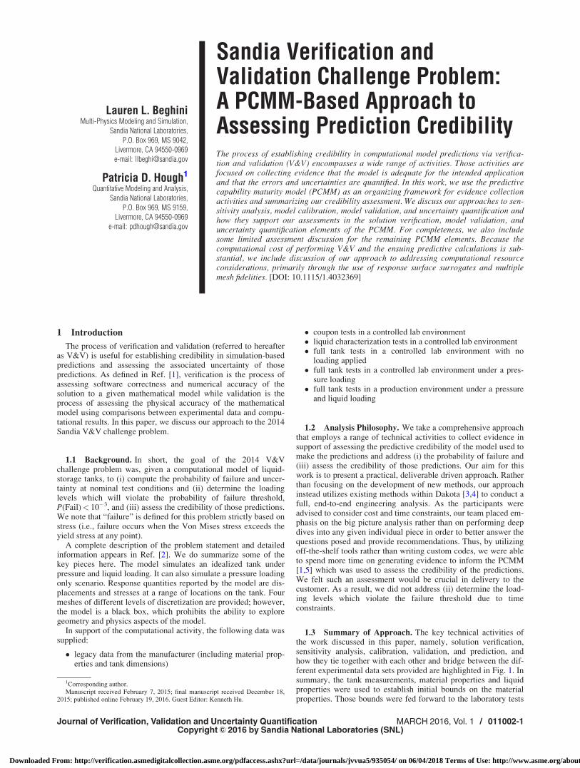
1.3 Summary of Approach. The key technical activities ofthe work discussed in this paper, namely, solution verification,sensitivity analysis, calibration, validation, and prediction, andhow they tie together with each other and bridge between the dif-ferent experimental data sets provided are highlighted in Fig. 1. Insummary, the tank measurements, material properties and liquidproperties were used to establish initial bounds on the materialproperties. Those bounds were fed forward to the laboratory tests

1Corresponding author.Manuscript received February 7, 2015; final manuscript received December 18,

2015; published online February 19, 2016. Guest Editor: Kenneth Hu.

Journal of Verification, Validation and Uncertainty Quantification MARCH 2016, Vol. 1 / 011002-1Copyright VC 2016 by Sandia National Laboratories (SNL)

Downloaded From: http://verification.asmedigitalcollection.asme.org/pdfaccess.ashx?url=/data/journals/jvvua5/935054/ on 06/04/2018 Terms of Use: http://www.asme.org/about-asme/terms-of-use

under controlled pressure to perform solution verification, sensi-tivity analysis, and a multifidelity calibration of the material prop-erties. Using the results of the calibration, the provided code wasthen used to simulate the field tests, which were validated againstthe field test data. Finally, predictions of the probability of failurewere made, and the credibility of those predictions was discussedin light of the evidence collected throughout the activities leadingup to the prediction. For all of these computational studies, wemake use of readily available methods in the Dakota softwarepackage [3].

The context in which we evaluate the credibility of the predic-tions we will ultimately make is the PCMM [1,5]. The PCMM is amodel which assesses the confidence one should place in the sim-ulation and its results through evaluation of the maturity level ofthe following six fundamental elements:

� geometric fidelity: level of detail included in the spatial andtemporal definition of the system

� physics fidelity: range of physics modeling fidelity rangingfrom empirical models to first-principles physics

� code verification: correctness of source code and numericalalgorithm

� solution verification: assessment of numerical solution errorsand confidence in computational results

� model validation: assessment of the physical accuracy of themodel by comparing the experimental data and computa-tional results

� uncertainty quantification: identification and characterizationof uncertainties, and thoroughness of sensitivity analysis todetermine sources of uncertainties

At the end of this paper, we will return to these elements and pro-vide an assessment and maturity level score associated with eachof these elements based on the evidence we generate as part of theanalysis activities. The maturity level scores can then be used toaid decision-making activities.

In Sec. 2, we discuss a sensitivity analysis we did for the pres-sure loading only scenario. This analysis is done across all meshfidelities in order to simultaneously address solution verificationand identification of driving model parameters. The intent is tobase our choice of mesh fidelity not just on error at the nominalchoice of parameter values but also on consistency of parametersensitivities. Section 3 describes our approach to calibration,which makes use of multiple model fidelities. The intent of thisactivity is primarily to refine our estimates of model parameterssuch that model predictions are consistent with experimental data.Additionally, this activity can support identification of modelform error and help inform distributions on model parameters.Section 4 describes validation of model predictions against dis-placement data collected in the field. This includes the use of a

polynomial chaos expansion (PCE) representation of model pre-dictions both to perform sensitivity analysis and to generate alarge number of instantiations over the parameter uncertaintiesto compute a broad range for errors between model and data.Section 5 discusses the probability of failure prediction, whichmakes use of a global reliability method based on a Gaussian pro-cess (GP) to incorporate parameter uncertainties in a computation-ally tractable way. Section 6 describes our assessment of thecredibility of the failure predictions in the context of the PCMM,and Sec. 7 concludes the paper with a final recommendation andsuggestions for future work that would further this effort.

2 Sensitivity Study and Solution Verification

The first step in our analysis was a sensitivity study conductedover the model parameters for the pressure-only model. Weincluded the mesh as a parameter in order to assess the importanceof the mesh discretization on the quantity of interest relative to themodel parameters and to inform our choice of mesh for the valida-tion and prediction elements of the analysis. The sensitivity studyalso serves as a screening of the parameters to identify those withthe most influence on the quantity of interest and thus those wewould want to include in model calibration and uncertainty quan-tification associated with validation and prediction.

For the purposes of the sensitivity study, we constructed toler-ance intervals [6,7] using the provided data on tank measure-ments, material properties, and liquid properties in order toestablish initial bounds on those model parameters. Given a num-ber of data samples, a tolerance interval provides the boundswithin which a specified percentage of the true population fallswith a specified amount of confidence. For this problem, we used99/90 tolerance intervals, i.e., the bounds in which 99% of thepopulation lies with 90% confidence. We used MINITAB [8] to com-pute the intervals. The MINITAB approach is based on Ref. [9],which defines the tolerance interval to be (l� kr, lþ kr), wherel is the sample mean, r is the standard deviation, and

k ¼

ffiffiffiffiffiffiffiffiffiffiffiffiffiffiffiffiffiffiffiffiffiffiffiffiffiffiffiffiffiffiffiffiffiffiffiffi� 1þ 1

N

� �z2

1�pð Þ=2

v21�c;�

vuuut(1)

N is the number of samples, v21�c;� is the critical value of the chi-

square distribution with degrees of freedom � that is exceededwith probability c, and z(1�p)/2 is the critical value of the normaldistribution associated with cumulative probability (1� p)/2. Wenote that much of this notation duplicates that used to define thematerial properties. We do this to remain consistent with commonnotation used for tolerance interval definition. This is the onlyplace in the paper where the notation takes on these meanings; thematerial property definitions apply everywhere else. While thisapproach makes a normality assumption that we cannot confirmgiven the very small amount of data, normality tests indicate thatwe cannot rule out a normal distribution. Furthermore, Ref. [10]argues that this approach more reliably estimates conservativebounds when data is scarce than other approaches and other distri-butions. The bounds we obtained for the model parameters are asfollows:

� E � [2.522� 107, 3.139� 107] (psi)� � � [0.250, 0.293]� L � [59.317, 61.926] (in.)� R � [29.221, 32.875] (in.)� T � [0.203, 0.263] (in.)w

We took pressure P � [27.911, 154.245] (psi) to encompass therange reported in the pressure-only lab tests plus the 5% measure-ment error.

To establish the relationship between model fidelities, a smallinitial Latin hypercube sampling (LHS) [11] study over the afore-mentioned parameters was conducted at each level of mesh

Fig. 1 This figure shows the flow of information from experi-mental data through to predictions about tank failure. Key activ-ities in the collection of credibility evidence are noted.

011002-2 / Vol. 1, MARCH 2016 Transactions of the ASME


discretization. More specifically, we took an incremental LHSapproach that allowed us to progressively double the sample sizein such a way that reused existing samples and that generated anew LHS sample that preserved the stratification and correlationstructures of the original sample. The total number of simulationsruns using this approach were:

� mesh 4 (finest)¼ 8 runs� mesh 3¼ 16 runs� mesh 2¼ 32 runs� mesh 1 (coarsest)¼ 64 runs

Note that the number of runs was increased as the mesh discretiza-tion decreased. Because more runs can be accommodated withfaster run times, we did this as a means of having as large a basisof comparison from one mesh level to the next as possible as wellas putting in place the information needed to generate surrogatesfor further analysis once a mesh has been chosen. The minimumnumber of samples required to establish linear correlations is onemore than the number of parameters. Given that we were consid-ering six model parameters, we chose eight as the initial samplesize and ran all meshes at those samples. We then doubled thenumber of samples via the incremental LHS approach to get thenext set at which to run meshes 1–3, bringing those to a total of16 samples. We repeated this process until we reached thereported number of samples for the remaining two meshes. Givenexperience-based projections of the level of parallelism we couldleverage for each mesh, the number of runs we could do simulta-neously, and the throughput of the available computing platforms,we determined this allocation of samples to be consistent withwhat could be completed in a week to 10 days of time. The gen-eral observations of the study were as follows:

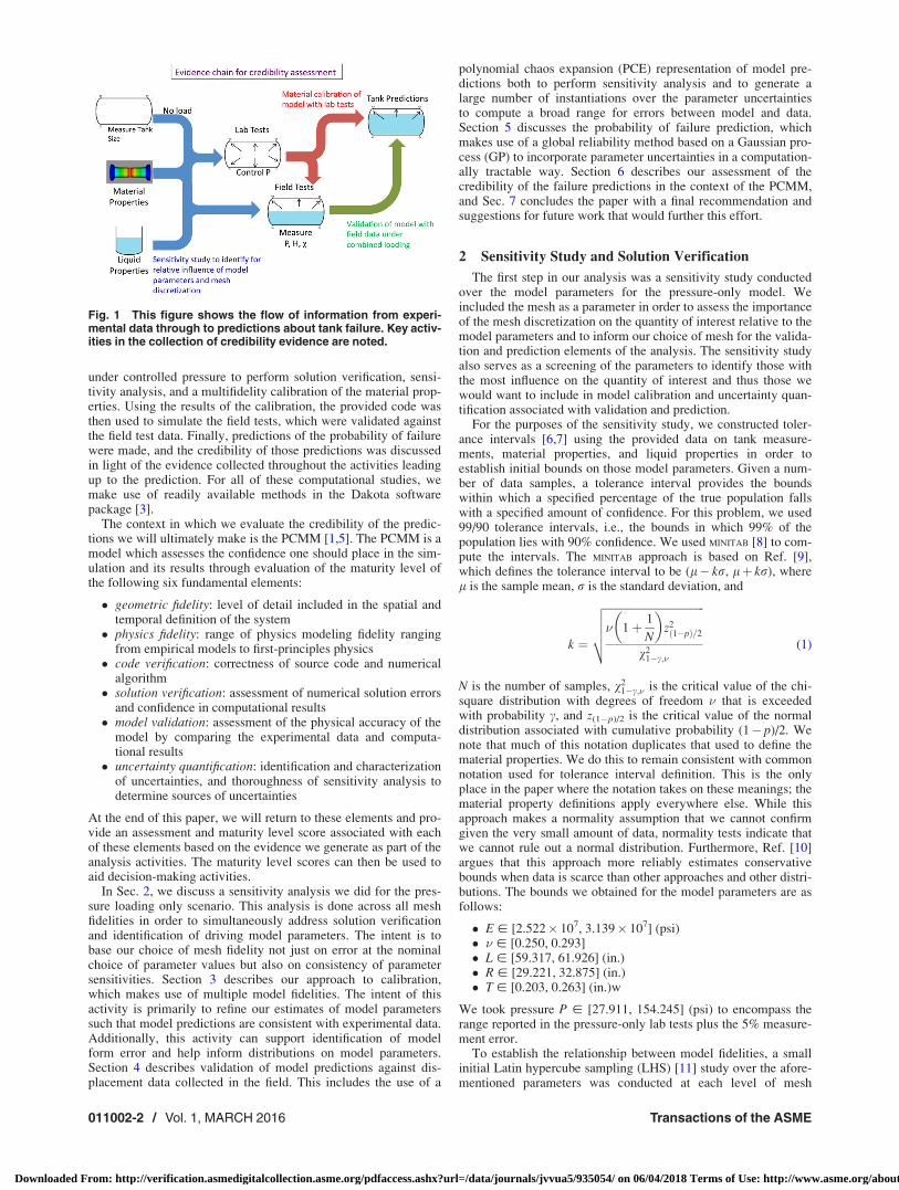
� As maximum stress and displacement values are the quanti-ties of interest for the failure predictions that will need to bemade, we examined the consistency of these values acrossmeshes and found them to be consistent across fidelities.Maximum stress results for mesh 2 and mesh 3 appear inFig. 2. Other mesh-to-mesh comparisons are similar, as arecomparable comparisons for displacements at locationswhere lab measurements were taken.

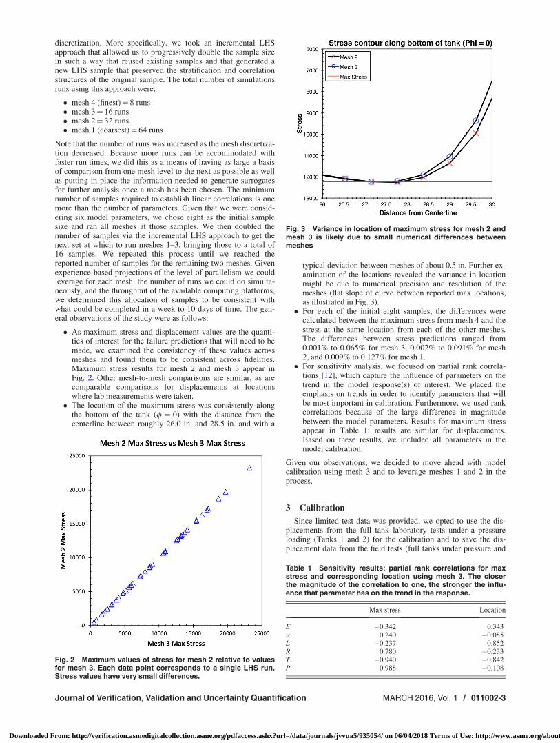
� The location of the maximum stress was consistently alongthe bottom of the tank (/ ¼ 0) with the distance from thecenterline between roughly 26.0 in. and 28.5 in. and with a

typical deviation between meshes of about 0.5 in. Further ex-amination of the locations revealed the variance in locationmight be due to numerical precision and resolution of themeshes (flat slope of curve between reported max locations,as illustrated in Fig. 3).

� For each of the initial eight samples, the differences werecalculated between the maximum stress from mesh 4 and thestress at the same location from each of the other meshes.The differences between stress predictions ranged from0.001% to 0.065% for mesh 3, 0.002% to 0.091% for mesh2, and 0.009% to 0.127% for mesh 1.

� For sensitivity analysis, we focused on partial rank correla-tions [12], which capture the influence of parameters on thetrend in the model response(s) of interest. We placed theemphasis on trends in order to identify parameters that willbe most important in calibration. Furthermore, we used rankcorrelations because of the large difference in magnitudebetween the model parameters. Results for maximum stressappear in Table 1; results are similar for displacements.Based on these results, we included all parameters in themodel calibration.

Given our observations, we decided to move ahead with modelcalibration using mesh 3 and to leverage meshes 1 and 2 in theprocess.

3 Calibration

Since limited test data was provided, we opted to use the dis-placements from the full tank laboratory tests under a pressureloading (Tanks 1 and 2) for the calibration and to save the dis-placement data from the field tests (full tanks under pressure and

Fig. 2 Maximum values of stress for mesh 2 relative to valuesfor mesh 3. Each data point corresponds to a single LHS run.Stress values have very small differences.

Fig. 3 Variance in location of maximum stress for mesh 2 andmesh 3 is likely due to small numerical differences betweenmeshes

Table 1 Sensitivity results: partial rank correlations for maxstress and corresponding location using mesh 3. The closerthe magnitude of the correlation to one, the stronger the influ-ence that parameter has on the trend in the response.

Max stress Location

E �0.342 0.343� 0.240 �0.085L �0.237 0.852R 0.780 �0.233T �0.940 �0.842P 0.988 �0.108

Journal of Verification, Validation and Uncertainty Quantification MARCH 2016, Vol. 1 / 011002-3


liquid loading—Tanks 3–6) for the validation. The specific objec-tive was to find model parameter values that would yield predicteddisplacements that most closely fit, on average, those measured inthe lab tests. The fit is formulated as a sum of squared displace-ment differences calculated across all measurement locations, i.e.,a nonlinear least-squares objective, with model parameter boundsdefined by the tolerance intervals identified in Sec. 2. To performthe calibration using Dakota, we used a multistart nonlinear least-squares solver, NL2SOL [13] with ten unique starting points. Thisallowed us to find possible multiple local minima, correspondingto multiple acceptable sets of nominal values for the modelparameters.

Based on our observations regarding the consistent trends indisplacement predictions across model fidelities, we incorporateda multifidelity approach in our calibration in order to reduce thenumber of expensive (mesh 3) simulations that needed to be done.For each step of the process, we report the total number of runsrequired for a given mesh discretization. We note that this totalis computed over all ten optimizations (one for each startingpoint) and includes the simulations done to compute finite-difference gradients. We additionally note that we leveragedthe independence of the computations and performed themsimultaneously in order to reduce the time required. The stepswere as follows:

(1) Using ten starting points, calibrate mesh 1 against all data(327 runs).

(2) Feed mesh 1 solutions (see Table 2) forward to calibratemesh 2 against all data (243 runs).

(3) Feed mesh 2 solutions (see Table 2) forward to calibratemesh 3 against all data (168 runs).

One might expect larger reductions in the number of simulationsrequired from one calibration level to the next; however, somenoise in the least-squares objective function caused by small

interacting changes in individual residuals leads to extra stepsneeded by the optimization method to reach the convergence cri-teria. Even so, without this multifidelity approach, we estimatedthat we would have needed around 400 simulations with the mesh3 model. The solutions for all three steps are reported in Table 2.The final total residuals for all of these solutions fell in the follow-ing range:

res 2 ð9:0� 10�3; 1:2� 10�2Þ

This small range indicates that all solutions found are roughlyequivalent and that the residual landscape is likely fairly flat (withsome noise) in the region containing these solutions. As a result,there is little evidence for narrowing the original parameterranges.

In addition to considering the point solutions computed usingthe deterministic nonlinear least squares solver NL2SOL [13] inDakota, we also examined the 95% confidence intervals for theindividual optimal parameters. We do not report the confidenceintervals for all of the solutions here, but we note that the intervalsbecame smaller after each step of the calibration processdescribed above. The following confidence intervals are typical ofwhat we observed for all of the solutions obtained using mesh 3:

� E � [�5.098� 109, 5.158� 109] (psi)� � � [�24.397, 24.965]� L � [57.911, 61.102] (in.)� R � [�2.442� 103, 2.5028� 103] (in.)� T � [�9.621, 10.071] (in.)

With the exception of the length parameter, these intervals areclearly unrealistically large and encompass parameter values thatare not physically meaningful. This could be the result of insuffi-ciencies in the experimental data, insufficiencies in the model, orerrors in confidence interval computation due to nonlinearities.Regardless, we were unable to derive useful information fromthese confidence intervals to further inform bounds or uncertaintycharacterizations for the model parameters. As such, the resultsleave open questions as to whether or not the experimental data isadequate to inform the calibration computation and whether or notthere is model form uncertainty that should be characterized. Bothclearly point to the need for further investigation.

In addition to computational savings, the multistart approachafforded us additional opportunities to explore the local minima.As a result, we found an inconsistency between the solutions andthe material data. In the course of trying to understand the experi-mental data, we examined the measurements taken from the cou-pons, shown in Table 3, for correlations between the properties.Figure 4 shows a positive correlation we observed betweenYoung’s modulus and the tank thickness. The results of the cali-bration, however, demonstrate the inverse trend. Measurements ofYoung’s modulus and thickness were taken independently, andphysical intuition provides no basis for believing that there wouldnecessarily be a relationship between Young’s modulus and thick-ness, so this brings into question whether or not there is some

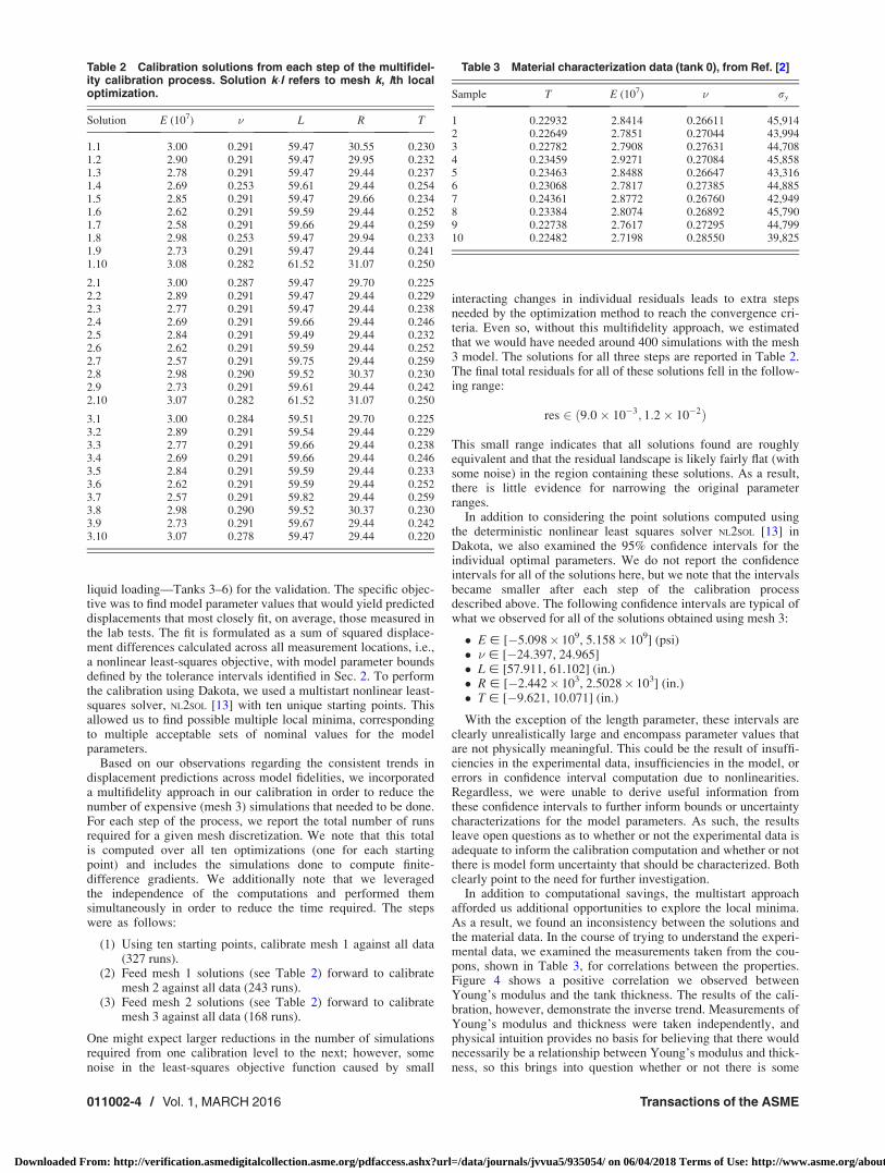
Table 2 Calibration solutions from each step of the multifidel-ity calibration process. Solution k�l refers to mesh k, lth localoptimization.

Solution E (107) � L R T

1.1 3.00 0.291 59.47 30.55 0.2301.2 2.90 0.291 59.47 29.95 0.2321.3 2.78 0.291 59.47 29.44 0.2371.4 2.69 0.253 59.61 29.44 0.2541.5 2.85 0.291 59.47 29.66 0.2341.6 2.62 0.291 59.59 29.44 0.2521.7 2.58 0.291 59.66 29.44 0.2591.8 2.98 0.253 59.47 29.94 0.2331.9 2.73 0.291 59.47 29.44 0.2411.10 3.08 0.282 61.52 31.07 0.250

2.1 3.00 0.287 59.47 29.70 0.2252.2 2.89 0.291 59.47 29.44 0.2292.3 2.77 0.291 59.47 29.44 0.2382.4 2.69 0.291 59.66 29.44 0.2462.5 2.84 0.291 59.49 29.44 0.2322.6 2.62 0.291 59.59 29.44 0.2522.7 2.57 0.291 59.75 29.44 0.2592.8 2.98 0.290 59.52 30.37 0.2302.9 2.73 0.291 59.61 29.44 0.2422.10 3.07 0.282 61.52 31.07 0.250

3.1 3.00 0.284 59.51 29.70 0.2253.2 2.89 0.291 59.54 29.44 0.2293.3 2.77 0.291 59.66 29.44 0.2383.4 2.69 0.291 59.66 29.44 0.2463.5 2.84 0.291 59.59 29.44 0.2333.6 2.62 0.291 59.59 29.44 0.2523.7 2.57 0.291 59.82 29.44 0.2593.8 2.98 0.290 59.52 30.37 0.2303.9 2.73 0.291 59.67 29.44 0.2423.10 3.07 0.278 59.47 29.44 0.220

Table 3 Material characterization data (tank 0), from Ref. [2]

Sample T E (107) � ry

1 0.22932 2.8414 0.26611 45,9142 0.22649 2.7851 0.27044 43,9943 0.22782 2.7908 0.27631 44,7084 0.23459 2.9271 0.27084 45,8585 0.23463 2.8488 0.26647 43,3166 0.23068 2.7817 0.27385 44,8857 0.24361 2.8772 0.26760 42,9498 0.23384 2.8074 0.26892 45,7909 0.22738 2.7617 0.27295 44,79910 0.22482 2.7198 0.28550 39,825



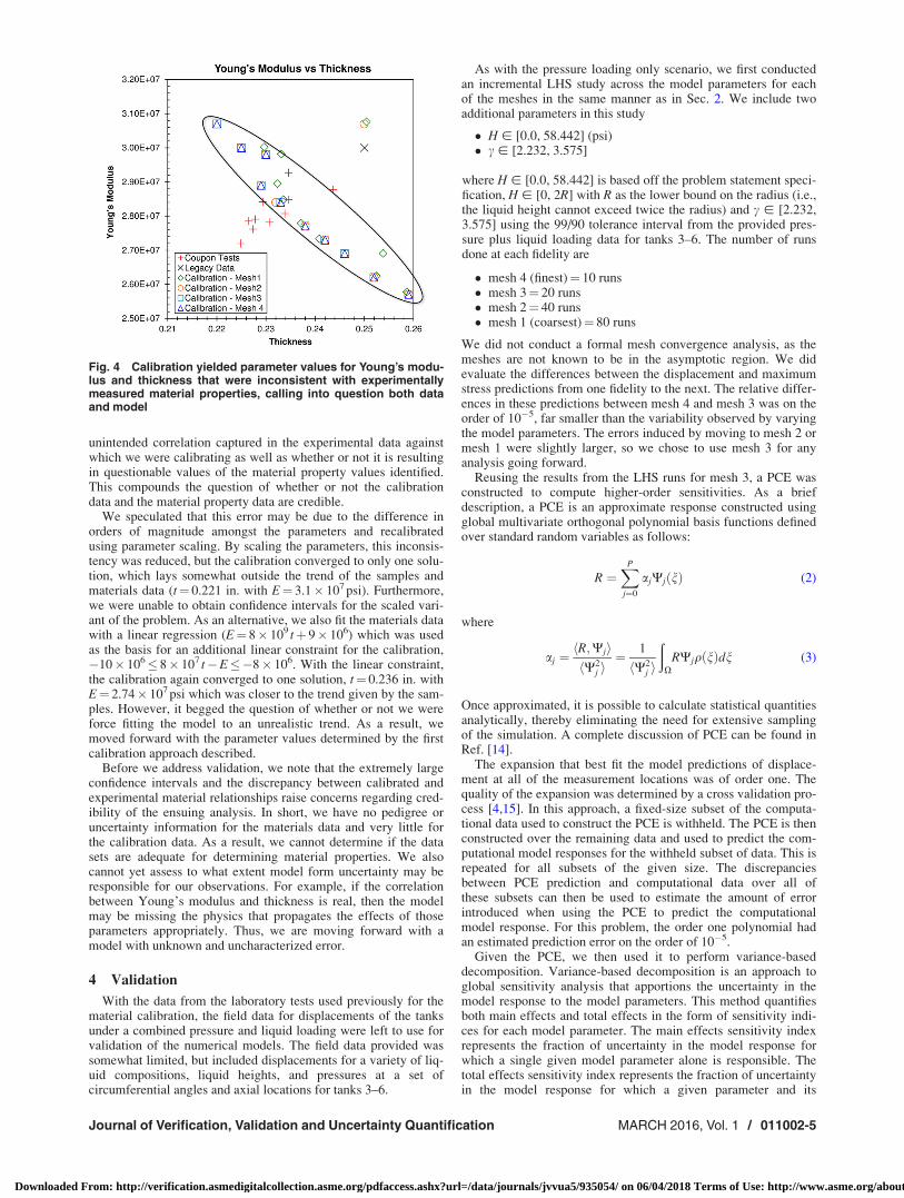
unintended correlation captured in the experimental data againstwhich we were calibrating as well as whether or not it is resultingin questionable values of the material property values identified.This compounds the question of whether or not the calibrationdata and the material property data are credible.

We speculated that this error may be due to the difference inorders of magnitude amongst the parameters and recalibratedusing parameter scaling. By scaling the parameters, this inconsis-tency was reduced, but the calibration converged to only one solu-tion, which lays somewhat outside the trend of the samples andmaterials data (t¼ 0.221 in. with E¼ 3.1� 107 psi). Furthermore,we were unable to obtain confidence intervals for the scaled vari-ant of the problem. As an alternative, we also fit the materials datawith a linear regression (E¼ 8� 109 tþ 9� 106) which was usedas the basis for an additional linear constraint for the calibration,�10� 106� 8� 107 t�E��8� 106. With the linear constraint,the calibration again converged to one solution, t¼ 0.236 in. withE¼ 2.74� 107 psi which was closer to the trend given by the sam-ples. However, it begged the question of whether or not we wereforce fitting the model to an unrealistic trend. As a result, wemoved forward with the parameter values determined by the firstcalibration approach described.

Before we address validation, we note that the extremely largeconfidence intervals and the discrepancy between calibrated andexperimental material relationships raise concerns regarding cred-ibility of the ensuing analysis. In short, we have no pedigree oruncertainty information for the materials data and very little forthe calibration data. As a result, we cannot determine if the datasets are adequate for determining material properties. We alsocannot yet assess to what extent model form uncertainty may beresponsible for our observations. For example, if the correlationbetween Young’s modulus and thickness is real, then the modelmay be missing the physics that propagates the effects of thoseparameters appropriately. Thus, we are moving forward with amodel with unknown and uncharacterized error.

4 Validation

With the data from the laboratory tests used previously for thematerial calibration, the field data for displacements of the tanksunder a combined pressure and liquid loading were left to use forvalidation of the numerical models. The field data provided wassomewhat limited, but included displacements for a variety of liq-uid compositions, liquid heights, and pressures at a set ofcircumferential angles and axial locations for tanks 3–6.

As with the pressure loading only scenario, we first conductedan incremental LHS study across the model parameters for eachof the meshes in the same manner as in Sec. 2. We include twoadditional parameters in this study

� H � [0.0, 58.442] (psi)� c � [2.232, 3.575]

where H � [0.0, 58.442] is based off the problem statement speci-fication, H � [0, 2R] with R as the lower bound on the radius (i.e.,the liquid height cannot exceed twice the radius) and c � [2.232,3.575] using the 99/90 tolerance interval from the provided pres-sure plus liquid loading data for tanks 3–6. The number of runsdone at each fidelity are

� mesh 4 (finest)¼ 10 runs� mesh 3¼ 20 runs� mesh 2¼ 40 runs� mesh 1 (coarsest)¼ 80 runs

We did not conduct a formal mesh convergence analysis, as themeshes are not known to be in the asymptotic region. We didevaluate the differences between the displacement and maximumstress predictions from one fidelity to the next. The relative differ-ences in these predictions between mesh 4 and mesh 3 was on theorder of 10�5, far smaller than the variability observed by varyingthe model parameters. The errors induced by moving to mesh 2 ormesh 1 were slightly larger, so we chose to use mesh 3 for anyanalysis going forward.

Reusing the results from the LHS runs for mesh 3, a PCE wasconstructed to compute higher-order sensitivities. As a briefdescription, a PCE is an approximate response constructed usingglobal multivariate orthogonal polynomial basis functions definedover standard random variables as follows:

R ¼XP

j¼0

ajWjðnÞ (2)

where

aj ¼hR;WjihW2

j i¼ 1

hW2j i

ðX

RWjq nð Þdn (3)

Once approximated, it is possible to calculate statistical quantitiesanalytically, thereby eliminating the need for extensive samplingof the simulation. A complete discussion of PCE can be found inRef. [14].

The expansion that best fit the model predictions of displace-ment at all of the measurement locations was of order one. Thequality of the expansion was determined by a cross validation pro-cess [4,15]. In this approach, a fixed-size subset of the computa-tional data used to construct the PCE is withheld. The PCE is thenconstructed over the remaining data and used to predict the com-putational model responses for the withheld subset of data. This isrepeated for all subsets of the given size. The discrepanciesbetween PCE prediction and computational data over all ofthese subsets can then be used to estimate the amount of errorintroduced when using the PCE to predict the computationalmodel response. For this problem, the order one polynomial hadan estimated prediction error on the order of 10�5.

Given the PCE, we then used it to perform variance-baseddecomposition. Variance-based decomposition is an approach toglobal sensitivity analysis that apportions the uncertainty in themodel response to the model parameters. This method quantifiesboth main effects and total effects in the form of sensitivity indi-ces for each model parameter. The main effects sensitivity indexrepresents the fraction of uncertainty in the model response forwhich a single given model parameter alone is responsible. Thetotal effects sensitivity index represents the fraction of uncertaintyin the model response for which a given parameter and its

Fig. 4 Calibration yielded parameter values for Young’s modu-lus and thickness that were inconsistent with experimentallymeasured material properties, calling into question both dataand model



interactions with other model parameters are responsible. Moredetails can be found in Ref. [12]. Variance-based decompositionbased on sampling a computational model is typically computa-tionally intractable due to the large number of samples needed.However, it can be done extremely efficiently by analyticallycomputing the sensitivity indices using the PCE [4]. In this man-ner, we identified pressure as the parameter that most contributesto the variance (approximately 63%) in the displacement predic-tions. Young’s modulus (16%) and tank wall thickness (15%) arealso contributors. These are therefore the driving uncertainties wetook forward into our probability of failure predictions.

In addition to using the PCE-based sensitivity analysis to iden-tify the model parameters that most contribute to the uncertaintyin the predicted displacements, more extensive sampling over themodel parameters was conducted on the PCE. These displacementpredictions were compared to the experimental field data asfollows:

(1) For a given measurement location and instantiation ofmodel parameters, compute the relative difference betweenthe PCE prediction and one of the experimentalmeasurements.

(2) Repeat the first step for the PCE prediction (using the sameparameter instantiation) and each of the other experimentalmeasurements at that location.

(3) Repeat the first two steps with a new instantiation of param-eters for the PCE prediction.

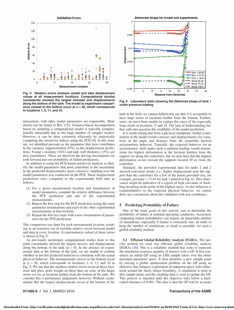
This comparison was done for each measurement location, result-ing in an extensive set of possible relative errors between modeland data at every location. A representative subset of those errorsis shown in Fig. 5.

As previously mentioned, computational studies done to thispoint consistently showed the largest stresses and displacementsalong the bottom of the tank (/ ¼ 0). In the absence of experi-mental data at the bottom of the tank, we are unable to confirmwhether or not this predicted behavior is consistent with the actualphysical behavior. The measurements closest to the bottom occurat / ¼ 30, which corresponds to locations 1, 6, 11, and 16 inFig. 5. We see that the smallest relative errors occur at those loca-tions and place more weight on these than on some of the largererrors we see at locations farther from the bottom of the tank. Weconsider this a preliminary judgement, however. Without confir-mation that the largest displacements occur at the bottom of the

tank in the field, we cannot definitively say that it is acceptable tohave large errors at locations farther from the bottom. Further-more, we have been unable to explain the cause of the especiallylarge errors at locations 17 and 18. The lack of understanding fur-ther calls into question the credibility of the model prediction.

It is worth noting that from a physical standpoint, further exam-ination of the model results (stresses and displacements) for varia-tions in the angle and distance from the centerline showedaxisymmetric behavior. Typically, the expected behavior for anaxisymmetric shell under such a uniform loading would demon-strate the highest deformation at the location furthest from thesupport (or along the centerline), but we note here that the highestdeformation occurs toward the supports located 30 in. from thecenterline.

Similarly, the provided experimental data for tanks 1 and 2showed consistent trends (i.e., higher displacement near the sup-port than the centerline) for a few of the points provided (see, forexample, pressure¼ 73.45 for tank 1 plotted in Fig. 6). This obser-vation might be indicative of a region of high curvature or buck-ling occurring at the point of the highest stress. As this behavior iscounterintuitive to the expected physical behavior, we cannotdraw any conclusions about the validation with any confidence.

5 Predicting Probability of Failure

One of the main goals of this activity was to determine theprobability of failure at nominal operating conditions. Accuratelycomputing failure probabilities can require an intractable numberof simulations, especially if failure is extremely rare. In order tokeep the number of simulations as small as possible, we used aglobal reliability method.

5.1 Efficient Global Reliability Analysis (EGRA). The spe-cific method we used was efficient global reliability analysis(EGRA) [16]. This is a reliability method that seeks to representthe simulation response quantity of interest with a GP. It first con-structs an initial GP using an LHS sample taken over the entireuncertain parameter space. It then identifies a new sample pointby solving a global optimization problem on the GP using anobjective that balances exploration of unknown space with refine-ment around the likely failure boundary. A simulation is done atthat sample point, and the resulting data is used to update the GP.This process is repeated until the objective falls below a hard-coded tolerance of 0.001. The idea is that the GP will be accurate

Fig. 6 Laboratory tests showing the deformed shape of tank 1under pressure loading

Fig. 5 Relative errors between model and data displacementvalues at all measurement locations. Computational studiesconsistently showed the largest stresses and displacementsalong the bottom of the tank. The model to experiment compari-sons closest to the bottom occur at / 5 30, which correspondsto locations 1, 6, 11, and 16.



near the failure boundary, thereby allowing accurate computationof the probability of failure. Unfortunately, however, a cross vali-dation error on the GP surrogate is not currently reported. The GPis trivial to evaluate, so the probability computation, which usesimportance sampling on the GP, becomes tractable. The targeted,iterative construction of the GP keeps the number of simulationsrequired to a minimum.

Since it is fundamental to EGRA, we here briefly define the GPsurrogate. The GP is a stochastic process defined by meanand covariance functions. It can have a constant, linear, or quad-ratic mean trend. The covariance function at points a and b isdefined as

Cov½ZðaÞ;ZðbÞ� ¼ r2ZRða;bÞ (4)

where r2Z is the process variance and R() is the following correla-

tion function:

Rða;bÞ ¼ exp �Xd

i¼1

hiðai � biÞ2" #

(5)

where d represents the problem dimension and hi is a scale param-eter, found by solving a maximum likelihood problem that indi-cates the correlation between the points in dimension i. A morecomplete introduction to GPs can be found in Ref. [17].

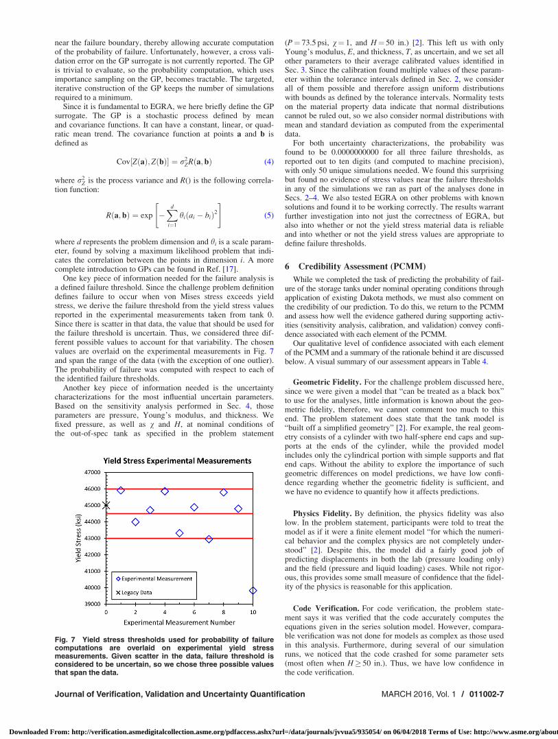
One key piece of information needed for the failure analysis isa defined failure threshold. Since the challenge problem definitiondefines failure to occur when von Mises stress exceeds yieldstress, we derive the failure threshold from the yield stress valuesreported in the experimental measurements taken from tank 0.Since there is scatter in that data, the value that should be used forthe failure threshold is uncertain. Thus, we considered three dif-ferent possible values to account for that variability. The chosenvalues are overlaid on the experimental measurements in Fig. 7and span the range of the data (with the exception of one outlier).The probability of failure was computed with respect to each ofthe identified failure thresholds.

Another key piece of information needed is the uncertaintycharacterizations for the most influential uncertain parameters.Based on the sensitivity analysis performed in Sec. 4, thoseparameters are pressure, Young’s modulus, and thickness. Wefixed pressure, as well as v and H, at nominal conditions ofthe out-of-spec tank as specified in the problem statement

(P¼ 73.5 psi, v¼ 1, and H¼ 50 in.) [2]. This left us with onlyYoung’s modulus, E, and thickness, T, as uncertain, and we set allother parameters to their average calibrated values identified inSec. 3. Since the calibration found multiple values of these param-eter within the tolerance intervals defined in Sec. 2, we considerall of them possible and therefore assign uniform distributionswith bounds as defined by the tolerance intervals. Normality testson the material property data indicate that normal distributionscannot be ruled out, so we also consider normal distributions withmean and standard deviation as computed from the experimentaldata.

For both uncertainty characterizations, the probability wasfound to be 0.0000000000 for all three failure thresholds, asreported out to ten digits (and computed to machine precision),with only 50 unique simulations needed. We found this surprisingbut found no evidence of stress values near the failure thresholdsin any of the simulations we ran as part of the analyses done inSecs. 2–4. We also tested EGRA on other problems with knownsolutions and found it to be working correctly. The results warrantfurther investigation into not just the correctness of EGRA, butalso into whether or not the yield stress material data is reliableand into whether or not the yield stress values are appropriate todefine failure thresholds.

6 Credibility Assessment (PCMM)

While we completed the task of predicting the probability of fail-ure of the storage tanks under nominal operating conditions throughapplication of existing Dakota methods, we must also comment onthe credibility of our prediction. To do this, we return to the PCMMand assess how well the evidence gathered during supporting activ-ities (sensitivity analysis, calibration, and validation) convey confi-dence associated with each element of the PCMM.

Our qualitative level of confidence associated with each elementof the PCMM and a summary of the rationale behind it are discussedbelow. A visual summary of our assessment appears in Table 4.

Geometric Fidelity. For the challenge problem discussed here,since we were given a model that “can be treated as a black box”to use for the analyses, little information is known about the geo-metric fidelity, therefore, we cannot comment too much to thisend. The problem statement does state that the tank model is“built off a simplified geometry” [2]. For example, the real geom-etry consists of a cylinder with two half-sphere end caps and sup-ports at the ends of the cylinder, while the provided modelincludes only the cylindrical portion with simple supports and flatend caps. Without the ability to explore the importance of suchgeometric differences on model predictions, we have low confi-dence regarding whether the geometric fidelity is sufficient, andwe have no evidence to quantify how it affects predictions.

Physics Fidelity. By definition, the physics fidelity was alsolow. In the problem statement, participants were told to treat themodel as if it were a finite element model “for which the numeri-cal behavior and the complex physics are not completely under-stood” [2]. Despite this, the model did a fairly good job ofpredicting displacements in both the lab (pressure loading only)and the field (pressure and liquid loading) cases. While not rigor-ous, this provides some small measure of confidence that the fidel-ity of the physics is reasonable for this application.

Code Verification. For code verification, the problem state-ment says it was verified that the code accurately computes theequations given in the series solution model. However, compara-ble verification was not done for models as complex as those usedin this analysis. Furthermore, during several of our simulationruns, we noticed that the code crashed for some parameter sets(most often when H� 50 in.). Thus, we have low confidence inthe code verification.

Fig. 7 Yield stress thresholds used for probability of failurecomputations are overlaid on experimental yield stressmeasurements. Given scatter in the data, failure threshold isconsidered to be uncertain, so we chose three possible valuesthat span the data.



Solution Verification. Solution verification is the one elementfor which we can express reasonably high confidence. While wedid not complete a formal convergence study, we did assess theeffects of mesh discretization on the displacement and stress pre-dictions. The relationship between meshes was well understood,and our initial LHS studies demonstrated very small changes andtrend consistencies in the maximum stresses and displacementsacross fidelities.

Model Validation. While validation using the experimentaldata was completed, conclusions that can be drawn are somewhatlimited, as displacements were provided for the field tests only atthe noncritical locations (circumferential angles, / 2 ½30; 150�,rather than along the bottom of the tanks, / ¼ 0 where the modelreported the highest stresses and displacements). That being said,we did find the best agreement between model and data at/ ¼ 30, the location closest to the bottom of the tank, so there issome small amount of confidence that can be placed in thevalidation.

Uncertainty Quantification. Some uncertainty quantificationwas conducted, but incorporation of the experimental data uncer-tainty was incomplete. Measurement uncertainties, including dis-placement measurements (presumed to be within 3%); pressuremeasurements (within 5% but no additional documentation onconfidence level), liquid height (varying with axial position due totank orientation) and v measurements (within 0.05 mass fraction),in particular, were not factored into the analysis. These uncertain-ties are, for the most part, an order of magnitude smaller thanthose that were included. Thus, we expect they will not changeany of our conclusions. Additionally, we did not include errors inthe response surface surrogates nor did we aggregate all of theuncertainties together in the final probability of failure predic-tions. Finally, the calibration activity revealed little information torefine experimentally determined uncertainty characterizations ofthe model parameters and identified possible model form uncer-tainty that needs exploration.

7 Conclusions and Future Work

The approach described in this work demonstrated a practical,project driven response to the challenge problem. By utilizing cur-rently available tools rather than developing our own, we wereconstrained by what methods were easily available throughDakota as well as by what information they report, but we wereable to perform a more comprehensive analysis and to betterunderstand both the experimental and the computational data. Inour case, the benefits were (1) a wider range of analysis tools atour disposal that could be used within the time constraints, (2) awell-informed assessment of the analysis credibility, and (3) theability to identify avenues for future work that would strengthenthe analysis.

7.1 Conclusions. Though we reported a zero probability offailure (to ten digits), we are skeptical about whether the yieldstress data and threshold values are reliable and would recom-mend further investigation before drawing conclusions and mak-ing recommendations to the customer. Based on our engineeringjudgement and PCMM (discussed previously), we note that thecredibility of some data, computations, or both is questionablethroughout this process. The most substantial of these include:

� possibly unrealistic correlation in calibration data� excessively large confidence intervals on calibration parame-

ter estimates� unknown and uncharacterized model form error� lack of experimental data at the bottom of the tank� nonintuitive “buckling” behavior� unknown error in the GP surrogate used for probability of

failure prediction

Thus, we report our overall confidence in the failure predictionsas low to medium. As such, we would consider it unwise to baseany decisions solely on these predictions. However, the support-ing sensitivity, calibration, and validation activities did yieldinsights into future work that would improve the credibility of themodel. Those suggestions are described in Sec. 7.2.

Table 4 Summary of our PCMM assessment: The darkest shade of gray is the target requirement. The second darkest does notmeet the requirement by one level, the third does not meet it by two levels, and the lightest does not meet it by three levels.

Element Maturity level 0 Maturity level 1 Maturity level 2 Maturity level 3

Representation andgeometric fidelity

Model built offsimplified geometry

Physics fidelity Numerical behaviorand physics notcompletely understood

Predicted displacementswell

Code verification Computes equationsaccurately for lesscomplex models

Code crashed for someparameter sets

Solution verification Relationship betweenmeshes well understood

Small changes and trendconsistencies acrossmultiple fidelities

Model validation Displacements providedat noncritical locations solimited conclusions canbe drawn

Uncertainty quantification Conducted, but incomplete

Limited model parameter UQErrors in response surfacesurrogates not included



7.2 Suggestions for Future Work. Based on the activitiesdone in support of the tank failure assessment, we have three mainproposals for future work: one associated with calibration, onewith validation, and an additional failure assessment prediction.

A substantial red flag was raised during model calibration inthat the correlation between some of the material properties foundfor the model was the inverse of those represented in the materialsdata provided. It is critical that there be a follow up on the pedi-gree of the data to ensure that it was gathered and reported cor-rectly. Additionally, further investigation into the model andunderstanding of the physics is necessary to determine whether ornot model form uncertainty is the cause of the discrepancy.

The results of laboratory tests for the full tank under a pressureloading, in addition to the finite element model results, providedvaluable insight into the behavior of the tank system. We observedthat for each test, the model output that the angle, /, where themaximum stress occurred was always zero (along the bottom ofthe tank) and the corresponding maximum displacement was nearthe supports. A plot of the deformation curve and correspondingstress contour is shown in Fig. 8.

Based on the physical observations discussed in the validationsection, more studies should be conducted regarding possibleimperfections in the tank geometry or misalignment of the con-nections, which could lead to premature failure. To be able tomake such a decision in the future, we would need to prioritize

and request resources to address the most pressing model and dataneeds. For example, the displacement field should be experimen-tally sampled on tanks 3–6 along the bottom in the critical area offailure.

In addition to computing the probability of failure at nominalconditions, participants were also asked to determine the loadinglevels which will violate the probability of failure threshold,P(Fail)< 10�3. In order to determine if the operating regime is ac-ceptable, we propose an optimization approach. In particular, wewould seek to find the parameter values within the operating rangethat resulted in the highest probability of failure. This would bedone by nesting EGRA computations within the optimization iter-ations. If the highest probability of failure is less than 10�3, thenthe current operational range can be considered adequate to ensuresafety. If not, then we must discover the boundaries that are safe.This may be revealed as a side effect of the computations done forthe optimization but will likely require additional modelexploration.

Acknowledgment

The authors would like to thank Ken Hu for all of his hard workorganizing the V&V Challenge Problem activities and for makingsure the participants had multiple opportunities to interact withone another, George Orient for his efforts in putting together thesoftware and models used, and the other participants for stimulat-ing discussion and intriguing ideas. We would also like to thankthree anonymous referees for their helpful comments; they wereextremely useful in improving the transparency and completenessof the paper. Finally, we would like to thank the ASC V&V pro-gram under whose funding this work was performed.

This work was performed at Sandia National Laboratories. San-dia National Laboratories is a multiprogram laboratory managedand operated by Sandia Corporation, a wholly owned subsidiaryof Lockheed Martin Corporation, for the U.S. Department ofEnergy’s National Nuclear Security Administration underContract No. DE-AC04-94AL85000.

Nomenclature

d ¼ tank wall displacement, normal to the surfaceE ¼ Young’s modulusH ¼ liquid heightL ¼ lengthm ¼ mesh IDP ¼ gauge pressureR ¼ radiusT ¼ wall thicknessx ¼ axial locationc ¼ liquid specific weight� ¼ Poisson’s ratior ¼ Von Mises stress/ ¼ circumferential anglev ¼ liquid composition (mass fraction)

References[1] Oberkampf, W., and Roy, C., 2010, Verification and Validation in Scientific

Computing, Cambridge University Press, New York.[2] Hu, K., 2013, “2014 V&V Challenge: Problem Statement,” Sandia National

Laboratories, Albuquerque, NM and Livermore, CA, Technical Report No.SAND2013-10486P.

[3] Adams, B. M., Bauman, L. E., Bohnhoff, W. J., Dalbey, K. R., Eddy, J. P.,Ebeida, M. S., Eldred, M. S., Hough, P. D., Hu, K. T., Jakeman, J. D., Swiler,L. P., Stephens, J. A., Vigil, D. M., and Wildey, T. M., 2014, “Dakota, a Multi-level Parallel Object-Oriented Framework for Design Optimization, ParameterEstimation, Uncertainty Quantification, and Sensitivity Analysis: Version 6.1Users Manual,” Sandia National Laboratories, Albuquerque, NM, TechnicalReport No. SAND2014-4633.

[4] Adams, B., Ebeida, M., Eldred, M., Jakeman, J., Swiler, L., Bohnhoff, W.,Dalbey, K., Eddy, J., Hu, K., Vigil, D., Bauman, L., and Hough, P., 2011,“Dakota, a Multilevel Parallel Object-Oriented Framework for Design

Fig. 8 Deformed shape and corresponding stresses along thebottom of the tank



http://dx.doi.org/10.1017/CBO9780511760396

http://dx.doi.org/10.1017/CBO9780511760396

https://share.sandia.gov/vvcw/wp-content/uploads/2014/01/SAND2013-10486P.pdf

https://share.sandia.gov/vvcw/wp-content/uploads/2014/01/SAND2013-10486P.pdf

Optimization, Parameter Estimation, Uncertainty Quantification, and Sensitiv-ity Analysis,” Sandia National Laboratories, Albuquerque, NM and Livermore,CA, Technical Report No. SAND2011-9106.

[5] Oberkampf, W., Pilch, M., and Trucano, T., 2007, “Predictive CapabilityMaturity Model for Computational Modeling and Simulation,” Sandia NationalLaboratories, Albuquerque, NM and Livermore, CA, Technical Report No.SAND2007-5948.

[6] Montgomery, D., and Runger, G., 1994, Applied Statistics and Probability forEngineers, Wiley, New York.

[7] Hahn, G., and Meeker, W., 1991, Statistical Intervals—A Guide for Practi-tioners, Wiley, New York.

[8] Computer Software by Minitab, Inc., “Minitab 17 Statistical Software,”www.minitab.com

[9] Howe, W., 1969, “Two-Sided Tolerance Limits for Normal Populations—SomeImprovements,” J. Am. Stat. Assoc., 64(326), pp. 610–620.

[10] Romero, V., Swiler, L., Urbina, A., and Mullins, J., 2013, “A Comparison ofMethods for Representing Sparsely Sampled Random Quantities,” SandiaNational Laboratories, Albuquerque, NM and Livermore, CA, Technical ReportNo. SAND2013-4561.

[11] Iman, R. L., and Shortencarier, M. J., 1984, “A Fortran 77 Program and User’sGuide for the Generation of Latin Hypercube Samples for Use With ComputerModels,” Sandia National Laboratories, Albuquerque, NM, Technical ReportNo. NUREG/CR-3624, SAND83-2365.

[12] Saltelli, A., Tarantola, S., Compolongo, F., and Ratto, M., 2004, Sensitivity Anal-ysis in Practice: A Guide to Assessing Scientific Models, Wiley, New York.

[13] Dennis, J. E., Gay, D. M., and Welsch, R. E., 1981, “ALGORITHM 573:NL2SOL—An Adaptive Nonlinear Least-Squares Algorithm,” ACM Trans.Math. Software, 7(3), pp. 369–383.

[14] Xiu, D., 2010, Numerical Methods for Stochastic Computations: A SpectralMethod Approach, Princeton University Press, Princeton, NJ.

[15] Hastie, T., Tibshirani, R., and Friedman, J., 2001, The Elements of StatisticalLearning: Data Mining, Inference, and Prediction: With 200 Full-Color Illus-trations, Springer-Verlag, Berlin.

[16] Bichon, B., Eldred, M., Swiler, L., Mahadevan, S., and McFarland, J., 2008,“Efficient Global Reliability Analysis for Nonlinear Implicit PerformanceFunctions,” AIAA J., 46(10), pp. 2459–2468.

[17] MacKay, D., 1998, “Introduction to Gaussian Processes,” Neural Networks andMachine Learning, Vol. 168, C. M. Bishop, ed., Springer, Berlin, pp. 133–165.



http://prod.sandia.gov/techlib/access-control.cgi/2007/075948.pdf


www.minitab.com

http://dx.doi.org/10.1080/01621459.1969.10500999



http://www.osti.gov/scitech/servlets/purl/7091452/

http://www.osti.gov/scitech/servlets/purl/7091452/

http://dx.doi.org/10.1145/355958.355966

http://dx.doi.org/10.1145/355958.355966

http://dx.doi.org/10.1007/978-0-387-21606-5

http://dx.doi.org/10.1007/978-0-387-21606-5

http://dx.doi.org/10.1007/978-0-387-21606-5

http://dx.doi.org/10.2514/1.34321

sandia verification and validation challenge problem: a...

Documents