santa ana river water right applications for … ana river water right applications for supplemental...
TRANSCRIPT

1
Santa Ana River Water Right Applicationsfor Supplemental Water Supply
Testimony of Dr. Dennis E. WilliamsCalifornia State Water Resource Control BoardMay 2 - 4, 2007 Muni/Western Ex. 6-389
2Muni/Western Ex. 6-389
Testimony SummaryTestimony SummaryTestimony Summary
The Project Will Result In Significant Benefits
Related To Groundwater In The SBBA Including:
♦ Development of up to 200,000 acre-ft that would
otherwise flow out of the area without being put to
beneficial use
♦ Additional water conservation will provide drought
protection and less reliance on imported water
The Project Will Result In Significant Benefits The Project Will Result In Significant Benefits
Related To Groundwater In The SBBA Including:Related To Groundwater In The SBBA Including:
♦♦ Development of up to 200,000 acreDevelopment of up to 200,000 acre--ft that would ft that would
otherwise flow out of the area without being put to otherwise flow out of the area without being put to
beneficial usebeneficial use
♦♦ Additional water conservation will provide drought Additional water conservation will provide drought
protection and less reliance on imported waterprotection and less reliance on imported water

3Muni/Western Ex. 6-389
Testimony SummaryTestimony SummaryTestimony Summary
♦ Reduce liquefaction potential by keeping groundwater
levels > 50 ft below the land surface
♦ highly urbanized SBBA
♦ area is particularly susceptible to liquefaction
♦ adjacent to the San Andreas, San Jacinto and Cucamonga faults
♦ new evidence indicates that there is a build-up of strain on the
southern San Andreas fault that will ultimately result in a large
earthquake on both the San Andreas and San Jacinto faults
♦♦ Reduce liquefaction potential by keeping groundwater Reduce liquefaction potential by keeping groundwater
levels > 50 ft below the land surfacelevels > 50 ft below the land surface
♦♦ highly urbanized SBBAhighly urbanized SBBA
♦♦ area is particularly susceptible to liquefactionarea is particularly susceptible to liquefaction
♦♦ adjacent to the San Andreas, San Jacinto and Cucamonga faultsadjacent to the San Andreas, San Jacinto and Cucamonga faults
♦♦ new evidence indicates that there is a buildnew evidence indicates that there is a build--up of strain on the up of strain on the
southern San Andreas fault that will ultimately result in a largsouthern San Andreas fault that will ultimately result in a large e
earthquake on both the San Andreas and San Jacinto faults earthquake on both the San Andreas and San Jacinto faults

4Muni/Western Ex. 6-389
Testimony SummaryTestimony SummaryTestimony Summary
♦ Assist in improving the water quality of the SBBA:
♦ accelerate cleanup of the contaminant plumes
♦ expected that Scenario A will clean up the Newmark and Muscoy
PCE plumes three years faster than if there was no project
♦ expected that Scenario A will clean up the Norton/Redlands-
Crafton TCE plume five years faster than if there was no project
♦♦ Assist in improving the water quality of the SBBA: Assist in improving the water quality of the SBBA:
♦♦ accelerate cleanup of the contaminant plumesaccelerate cleanup of the contaminant plumes
♦♦ expected that Scenario A will clean up the Newmark and Muscoy expected that Scenario A will clean up the Newmark and Muscoy
PCE plumes three years faster than if there was no projectPCE plumes three years faster than if there was no project
♦♦ expected that Scenario A will clean up the Norton/Redlandsexpected that Scenario A will clean up the Norton/Redlands--
Crafton TCE plume five years faster than if there was no projectCrafton TCE plume five years faster than if there was no project

5Muni/Western Ex. 6-389
Testimony SummaryTestimony SummaryTestimony Summary
♦ The diverted water will have overall benefits with
respect to TDS and nitrate concentrations:
♦ for TDS, there would be beneficial impacts under the project
scenarios in the Bunker Hill A management zone
♦ less than significant TDS impacts expected in the Bunker Hill B
and Lytle management zones
♦ With respect to nitrate concentration, beneficial impacts would
be anticipated for all management zones
♦♦ The diverted water will have overall benefits with The diverted water will have overall benefits with
respect to TDS and nitrate concentrations:respect to TDS and nitrate concentrations:
♦♦ for TDS, there would be beneficial impacts under the project for TDS, there would be beneficial impacts under the project
scenarios in the Bunker Hill A management zonescenarios in the Bunker Hill A management zone
♦♦ less than significant TDS impacts expected in the Bunker Hill B less than significant TDS impacts expected in the Bunker Hill B
and Lytle management zones and Lytle management zones
♦♦ With respect to nitrate concentration, beneficial impacts would With respect to nitrate concentration, beneficial impacts would
be anticipated for all management zonesbe anticipated for all management zones

6Muni/Western Ex. 6-389
Testimony SummaryTestimony SummaryTestimony Summary
♦ The findings of my work was based on using six model
scenarios that were developed and tested with an
integrated groundwater and streamflow model, as well
as a solute transport model
♦ The ground water flow model simulates groundwater levels,
quantities, directions and rates of groundwater flow
♦ The solute transport model simulates water quality
concentrations (e.g. TDS, nitrate, perchlorate, PCE and TCE)
♦♦ The findings of my work was based on using six model The findings of my work was based on using six model
scenarios that were developed and tested with an scenarios that were developed and tested with an
integrated groundwater and streamflow model, as well integrated groundwater and streamflow model, as well
as a solute transport modelas a solute transport model
♦♦ The ground water flow model simulates groundwater levels, The ground water flow model simulates groundwater levels,
quantities, directions and rates of groundwater flowquantities, directions and rates of groundwater flow
♦♦ The solute transport model simulates water quality The solute transport model simulates water quality
concentrations (e.g. TDS, nitrate, perchlorate, PCE and TCE)concentrations (e.g. TDS, nitrate, perchlorate, PCE and TCE)
7Muni/Western Ex. 6-389
Testimony SummaryTestimony SummaryTestimony Summary
♦ The six model scenarios simulated the following
conditions:
♦ No Project
♦ Maximum capture (1,500 cfs)
♦ Minimum capture (500 cfs)
♦ Most likely scenario (1,500 cfs, which takes into account the
Seven Oaks Accord and the settlement agreement with the
Conservation District)
♦♦ The six model scenarios simulated the following The six model scenarios simulated the following
conditions:conditions:
♦♦ No ProjectNo Project
♦♦ Maximum capture (1,500 cfs)Maximum capture (1,500 cfs)
♦♦ Minimum capture (500 cfs)Minimum capture (500 cfs)
♦♦ Most likely scenario (1,500 cfs, which takes into account the Most likely scenario (1,500 cfs, which takes into account the
Seven Oaks Accord and the settlement agreement with the Seven Oaks Accord and the settlement agreement with the
Conservation District)Conservation District)

8Muni/Western Ex. 6-389
Testimony SummaryTestimony SummaryTestimony Summary
♦ A subsidence model was developed to evaluate project
impacts
♦ Analytical models were developed to examine impacts
of artificial recharge (i.e. spreading) in areas outside of
the SBBA
♦♦ A subsidence model was developed to evaluate project A subsidence model was developed to evaluate project
impactsimpacts
♦♦ Analytical models were developed to examine impacts Analytical models were developed to examine impacts
of artificial recharge (i.e. spreading) in areas outside of of artificial recharge (i.e. spreading) in areas outside of
the SBBAthe SBBA

9Muni/Western Ex. 6-389
Overview of Groundwater Models Overview of Groundwater Models Overview of Groundwater Models
♦ Brief Review of Groundwater Modeling Tasks
♦ Results of Groundwater Model Runs
♦ Discussion of Subsidence Modeling
♦ Impacts of Spreading Outside the Model Area
♦♦ Brief Review of Groundwater Modeling TasksBrief Review of Groundwater Modeling Tasks
♦♦ Results of Groundwater Model RunsResults of Groundwater Model Runs
♦♦ Discussion of Subsidence ModelingDiscussion of Subsidence Modeling
♦♦ Impacts of Spreading Outside the Model AreaImpacts of Spreading Outside the Model Area

10Muni/Western Ex. 6-389
Overview of Groundwater Models Overview of Groundwater Models Overview of Groundwater Models
♦ Brief Review of Groundwater Modeling Tasks
♦ Results of Groundwater Model Runs
♦ Discussion of Subsidence Modeling
♦ Impacts of Spreading Outside the Model Area
♦♦ Brief Review of Groundwater Modeling TasksBrief Review of Groundwater Modeling Tasks
♦♦ Results of Groundwater Model RunsResults of Groundwater Model Runs
♦♦ Discussion of Subsidence ModelingDiscussion of Subsidence Modeling
♦♦ Impacts of Spreading Outside the Model AreaImpacts of Spreading Outside the Model Area

11Muni/Western Ex. 6-389
Brief Review of Groundwater Modeling TasksBrief Review of Groundwater Modeling TasksBrief Review of Groundwater Modeling Tasks
♦ Purpose:
♦ To Evaluate Potential Impacts on Groundwater Levels and
♦ Quality in the San Bernardino Basin Area Due to Various
♦ Proposed Seven Oaks Reservoir Water Diversion Scenarios
♦ Types of Models:
♦ MODFLOW - Flow
♦ MODPATH - Particle Tracking
♦ MT3DMS - Solute Transport
♦ Model Calibration and Verification
♦ Model Scenarios
♦♦ Purpose:Purpose:
♦♦ To Evaluate Potential Impacts on Groundwater Levels and To Evaluate Potential Impacts on Groundwater Levels and
♦♦ Quality in the San Bernardino Basin Area Due to Various Quality in the San Bernardino Basin Area Due to Various
♦♦ Proposed Seven Oaks Reservoir Water Diversion ScenariosProposed Seven Oaks Reservoir Water Diversion Scenarios
♦♦ Types of Models:Types of Models:
♦♦ MODFLOW MODFLOW -- FlowFlow
♦♦ MODPATH MODPATH -- Particle TrackingParticle Tracking
♦♦ MT3DMS MT3DMS -- Solute TransportSolute Transport
♦♦ Model Calibration and VerificationModel Calibration and Verification
♦♦ Model ScenariosModel Scenarios

12Muni/Western Ex. 6-389
Location of Spreading BasinsLocation of Spreading BasinsLocation of Spreading Basins
East Twin Creek SG
City Creek SG
Santa Ana SG
Mill Creek SG
Wilson Basin SG
Gateway Wash
Cactus Basin SG
Patton Basins
SG
Waterman Basins SG
BadgerBasins SG
Devils Canyon & Sweetwater
Basins SGExisting
Lytle Creek SG
Muscoy
Newmark
Crafton-Redlands
NortonSanta Fe
Garden Air Creek SG

13Muni/Western Ex. 6-389
Contaminant Plumes in the Bunker Hill BasinContaminant Plumes in the Bunker Hill BasinContaminant Plumes in the Bunker Hill Basin
MuscoyPlume(PCE)
NewmarkPlume(PCE)
Santa FePlume
Crafton-RedlandsPlume (TCE)
NortonPlume(TCE)
14Muni/Western Ex. 6-389
Description of the USGS ModelDescription of the USGS ModelDescription of the USGS Model
Conceptual ModelConceptual Model
CONCEPTUAL MODEL
StreamStream
upper water-bearing zoneupper water-bearing zone
Layer 2Layer 2Layer 1Layer 1
Layer 2Layer 2
Layer 1Layer 1
middle and lower confining members and middle and lower water-bearing zones
middle and lower confining members and middle and lower water-bearing zones
FIELD CONDITIONS
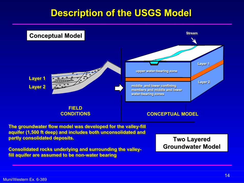
The groundwater flow model was developed for the valley-fill aquifer (1,500 ft deep) and includes both unconsolidated and partly consolidated deposits.
Consolidated rocks underlying and surrounding the valley-fill aquifer are assumed to be non-water bearing
The groundwater flow model was developed for the valley-fill aquifer (1,500 ft deep) and includes both unconsolidated and partly consolidated deposits.
Consolidated rocks underlying and surrounding the valley-fill aquifer are assumed to be non-water bearing
Two LayeredTwo LayeredGroundwater ModelGroundwater Model

15Muni/Western Ex. 6-389
Model Area and Grid LayoutModel Area and Grid LayoutModel Area and Grid Layout82
0 ft
1 184
118
1
820 ft
PUMPING & RECHARGE
INFLOW/OUTFLOWINFLOW/OUTFLOW
118 x 184 Cells/Layer118 x 184 Cells/LayerX 2 layersX 2 layers
(43,424 cells in total)

16Muni/Western Ex. 6-389
Model Layers Model Layers
Model Layer 1(100’-300’ ft thick)
Model Layer 2(400’-1000’ thick)
10 x Vertical Exaggeration
Seven Oaks Dam and ReservoirSeven Oaks Dam and Reservoir
SAR
View looking NE

17Muni/Western Ex. 6-389
Update of USGS ModelUpdate of USGS ModelUpdate of USGS Model
GROUNDWATER FLOW MODEL
4.93 percent4.92 percentRelative Error1
1945 - 20001945 - 1998Transient Calibration Period
same1945Steady-State Calibration Year
same1.2Time Step Multiplier
same100Number of Time Steps per Stress Period
same1 yearLength of Stress Period
same2Number of Layers
same118 (i-direction) and 184 (j-direction)Model Grid
same820 ft x 820 ft (uniform)Cell Size
same21,712 cells per layerSize
sameAll of the valley-fill within the Bunker Hill and Lytle Creek basins (approximately 524 sq. miles)
Areal Extent
sameMODFLOWModel Package
USGS Model (Updated)Original USGS ModelItem
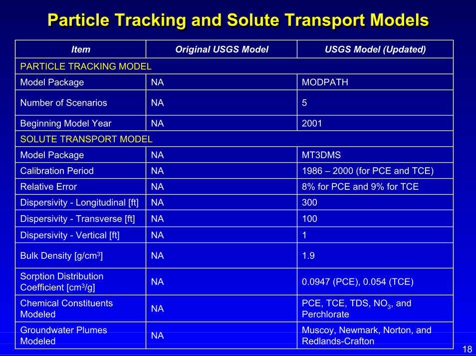
Particle Tracking and Solute Transport Models Particle Tracking and Solute Transport Models Particle Tracking and Solute Transport Models
8% for PCE and 9% for TCE NARelative Error
PARTICLE TRACKING MODEL
SOLUTE TRANSPORT MODEL
Muscoy, Newmark, Norton, and Redlands-CraftonNAGroundwater Plumes
Modeled
PCE, TCE, TDS, NO3, and PerchlorateNAChemical Constituents
Modeled
0.0947 (PCE), 0.054 (TCE)NASorption Distribution Coefficient [cm3/g]
1.9NABulk Density [g/cm3]
1NADispersivity - Vertical [ft]
100NADispersivity - Transverse [ft]
300NADispersivity - Longitudinal [ft]
1986 – 2000 (for PCE and TCE)NACalibration Period
MT3DMSNAModel Package
2001NABeginning Model Year
5NANumber of Scenarios
MODPATHNAModel Package
USGS Model (Updated)Original USGS ModelItem
18

19Muni/Western Ex. 6-389
Results show model Results show model captures long and shortcaptures long and short--term temporal trends in term temporal trends in
groundwater levelsgroundwater levels
Model Calibration HydrographsModel Calibration HydrographsModel Calibration Hydrographs

20Muni/Western Ex. 6-389
Statistical Measure of Calibration – Relative ErrorStatistical Measure of Calibration Statistical Measure of Calibration –– Relative ErrorRelative Error
♦ Relative Error (RE) = standard deviation of residuals (model water levels – observed) divided by the range of observed values
♦ An industry standard method commonly used to measure the degree of model calibration
♦ An acceptable RE is 10% or less ♦ Flow Model RE = 5%
♦ Solute Transport Models RE = 8%-9%
♦ Sources: Spitz and Moreno, 1996; Environmental Simulations, Inc., 1999
♦♦ Relative Error (RE) = standard deviation of residuals Relative Error (RE) = standard deviation of residuals (model water levels (model water levels –– observed) divided by the range of observed) divided by the range of observed valuesobserved values
♦♦ An industry standard method commonly used to An industry standard method commonly used to measure the degree of model calibration measure the degree of model calibration
♦♦ An acceptable RE is 10% or less An acceptable RE is 10% or less ♦♦ Flow Model RE = 5%Flow Model RE = 5%
♦♦ Solute Transport Models RE = 8%Solute Transport Models RE = 8%--9%9%
♦♦ Sources: Spitz and Moreno, 1996; Environmental Sources: Spitz and Moreno, 1996; Environmental Simulations, Inc., 1999Simulations, Inc., 1999

21Muni/Western Ex. 6-389
Hydrologic Base PeriodHydrologic Base PeriodHydrologic Base Period
♦ The Hydrologic “Base Period” was selected as the 39-year period from October 1961 through September 2000 (water years 1961/1962 – 1999/2000)
♦ The Hydrologic Base Period includes both wet and dry hydrologic cycles with an average hydrologic condition approximately the same as the long-term average
♦♦ The Hydrologic “Base Period” was selected as the The Hydrologic “Base Period” was selected as the 3939--year period from October 1961 through year period from October 1961 through September 2000 (water years 1961/1962 September 2000 (water years 1961/1962 –– 1999/2000) 1999/2000)
♦♦ The Hydrologic Base Period includes both wet and The Hydrologic Base Period includes both wet and dry hydrologic cycles with an average hydrologic dry hydrologic cycles with an average hydrologic condition approximately the same as the longcondition approximately the same as the long--term term average average

22Muni/Western Ex. 6-389
15
20
2530
35
2025 30
35
Long-Term Average Annual Rainfall (1870-1970)LongLong--Term Average Annual Rainfall (1870Term Average Annual Rainfall (1870--1970)1970)

Stations with more than 100 years of record:San Bernardino County Hospital, Redlands Facts and Big Bear Lake Dam
23

Average precipitation for water years 1962-2000
ranging from 95 to 99% of the long term average
(1870-1970)
For example, if 1962 is used as the start of the base period then the range of the 3 stations is approx 95-99% of the long-term average
(Based on Isohyetal Map)
24
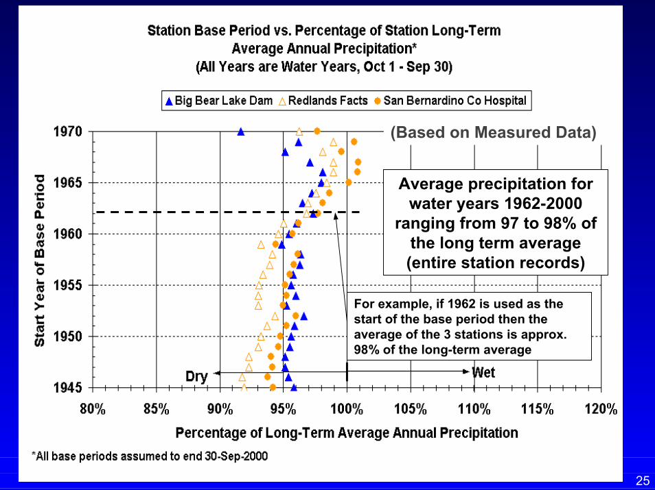
Average precipitation for water years 1962-2000
ranging from 97 to 98% of the long term average (entire station records)
For example, if 1962 is used as the start of the base period then the average of the 3 stations is approx. 98% of the long-term average
(Based on Measured Data)
25

Average streamflow for water years 1962-2000
was approximately 99% of the long term average
26

27Muni/Western Ex. 6-389
Water years 1962-2000 was selected as base period. This
period covers wet and dry cycles with an average of
approximately normal condition
19621962--2000 2000 (1(1--OctOct--61 through 3061 through 30--SepSep--00)00)
27

28Muni/Western Ex. 6-389
Hydrologic Base Period Meets All CriteriaHydrologic Base Period Meets All Criteria
-40
-30
-20
-10
0
10
20
30
40
50
1890
1894
1898
1902
1906
1910
1914
1918
1922
1926
1930
1934
1938
1942
1946
1950
1954
1958
1962
1966
1970
1974
1978
1982
1986
1990
1994
1998
2002
Water Year
Cum
ulat
ive
Dep
artu
re fr
om M
ean
Ann
ual P
reci
pita
tion
[inch
es]
1
3
2
4 4
Long-term average annual precipitation = 16.4 inches
1Average precipitation of the base period (16 in.) is approximately equal to the average precipitation of the long-term (1890-2000) record of 16.4 inches.
2Base period contains periods of wet, dry and average hydrologic conditions.
3Base period is sufficiently long (39 years) to contain data representative of the averages, deviations from the averages, and extreme values of the historical period from 1890 to 2000.
Base period is representative of recent and cultural condit ions (e.g., land use, urbanization, etc.)for the purpose of using the base period in forecasting models.
4Base period contains a dry trend at both the beginning and end of the period.
Base Period(WY 1961-62 through WY 1999-00)
Cumulative Departure from the Mean Annual
Source: San Bernardino County Flood Control 28
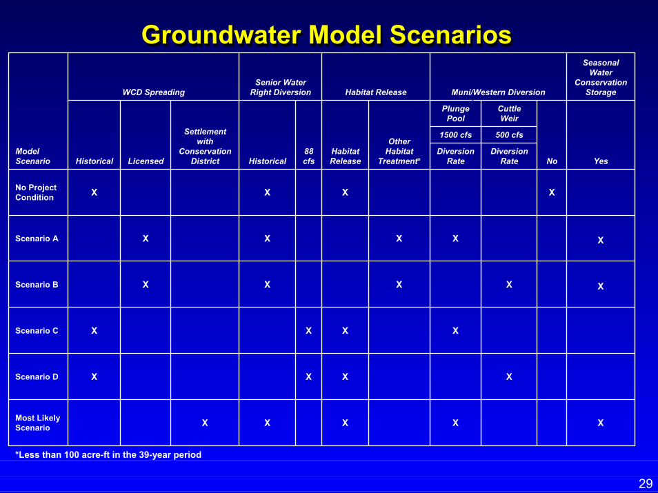
*Less than 100 acre-ft in the 39-year period
XXXXXMost Likely Scenario
XXXXScenario D
XXXXScenario C
XXXXXScenario B
XXXXXScenario A
XXXXNo Project Condition
Diversion Rate
Diversion Rate
500 cfs1500 cfs
YesNo
Cuttle Weir
Plunge Pool
Other Habitat
Treatment*Habitat Release
88 cfsHistorical
Settlement with
Conservation DistrictLicensedHistorical
Seasonal Water
Conservation StorageMuni/Western DiversionHabitat Release
Senior Water Right DiversionWCD Spreading
Model Scenario
Groundwater Model ScenariosGroundwater Model ScenariosGroundwater Model Scenarios
29

30Muni/Western Ex. 6-389
Overview of Groundwater Models Overview of Groundwater Models Overview of Groundwater Models
♦ Brief Review of Groundwater Modeling Tasks
♦ Results of Groundwater Model Runs
♦ Discussion of Subsidence Modeling
♦ Impacts of Spreading Outside the Model Area
♦♦ Brief Review of Groundwater Modeling TasksBrief Review of Groundwater Modeling Tasks
♦♦ Results of Groundwater Model RunsResults of Groundwater Model Runs
♦♦ Discussion of Subsidence ModelingDiscussion of Subsidence Modeling
♦♦ Impacts of Spreading Outside the Model AreaImpacts of Spreading Outside the Model Area
31Muni/Western Ex. 6-389
Results of Groundwater Model RunsResults of Groundwater Model RunsResults of Groundwater Model Runs
♦ Groundwater Elevations
♦ Areas of Potential Liquefaction
♦ Groundwater Budgets
♦ Groundwater Quality and Contamination
♦♦ Groundwater ElevationsGroundwater Elevations
♦♦ Areas of Potential LiquefactionAreas of Potential Liquefaction
♦♦ Groundwater BudgetsGroundwater Budgets
♦♦ Groundwater Quality and ContaminationGroundwater Quality and Contamination

32Muni/Western Ex. 6-389
Groundwater ElevationsGroundwater ElevationsGroundwater ElevationsNote: In forebay area, water levels are higher
w/projectProject
No Project
Note: In pressure zone, water levels are lower
w/projectProject
No Project

33Muni/Western Ex. 6-389
Areas of Potential LiquefactionAreas of Potential LiquefactionAreas of Potential Liquefaction
Depth to WaterDark Blue: <50 ftLight Blue: 50-70 ftLight Gray: >70 ft
No Project Condition Scenario A (Max Capture)
20
30 10
039 yrs
Wet
Wet
Wet
Wet
2001-2039

34Muni/Western Ex. 6-389
Cumulative Area of Potential Liquefaction 2001-2039Cumulative Area of Potential Liquefaction 2001Cumulative Area of Potential Liquefaction 2001--20392039
Reduction of 67%Reduction of 67%--21,45621,45610,72810,728Most Likely Most Likely ScenarioScenario
Reduction of 48%Reduction of 48%--15,35915,35916,82516,825Scenario DScenario D
Reduction of 77%Reduction of 77%--24,65124,6517,5337,533Scenario AScenario A
----32,18432,184No ProjectNo Project
CommentsCommentsChanges as Changes as
Compared to No Compared to No ProjectProject[acres][acres]
Cumulative Area Cumulative Area Susceptible to Susceptible to
Liquefaction in the Liquefaction in the Pressure ZonePressure Zone
[acres][acres]
Model Model ScenarioScenario

35Muni/Western Ex. 6-389
Recharge from Gaged
Streamflow
139,517Infiltration of
Direct Precipitation
1,137Recharge from
Ungaged Mountain Front
Runoff
17,820Recharge from Local Runoff Generated by Precipitation
5,627
Underflow Recharge
2,997
Artificial Recharge at
Other Spreading Grounds
21,932 Artificial Recharge At SAR Spreading
Grounds
10,384Return Flow from
Groundwater Pumping
39,575
Underflow Discharge
3,003
Evapotranspiration
5,822
GroundwaterPumping
233,488
INFLOW
OUTFLOW
Hydrologic Budget for Model Run No Project
Average of 2001 – 2039 (Units in acre-ft/yr)
EQUATION OF HYDROLOGIC EQUILIBRIUMINFLOW = OUTFLOW +/- CHANGE IN GROUNDWATER STORAGE
CHANGE IN GROUNDWATER STORAGE = -3,324 ACRE-FT/YR
Change inGroundwater
Storage
35

36Muni/Western Ex. 6-389
Recharge from Gaged
Streamflow
131,022Infiltration of
Direct Precipitation
1,137Recharge from
Ungaged Mountain Front
Runoff
17,820Recharge from Local Runoff Generated by Precipitation
5,627
Underflow Recharge
2,997
Artificial Recharge at
Other Spreading Grounds
39,172 Artificial Recharge At SAR Spreading
Grounds
4,961Return Flow from
Groundwater Pumping
39,614
Underflow Discharge
2,860
Evapotranspiration
6,314
GroundwaterPumping
236,582
INFLOW
OUTFLOW
Hydrologic Budget for Model Run Scenario A
Average of 2001 – 2039 (Units in acre-ft/yr)
EQUATION OF HYDROLOGIC EQUILIBRIUMINFLOW = OUTFLOW +/- CHANGE IN GROUNDWATER STORAGE
CHANGE IN GROUNDWATER STORAGE = -3,406 ACRE-FT/YR
Change inGroundwater
Storage
36
37Muni/Western Ex. 6-389
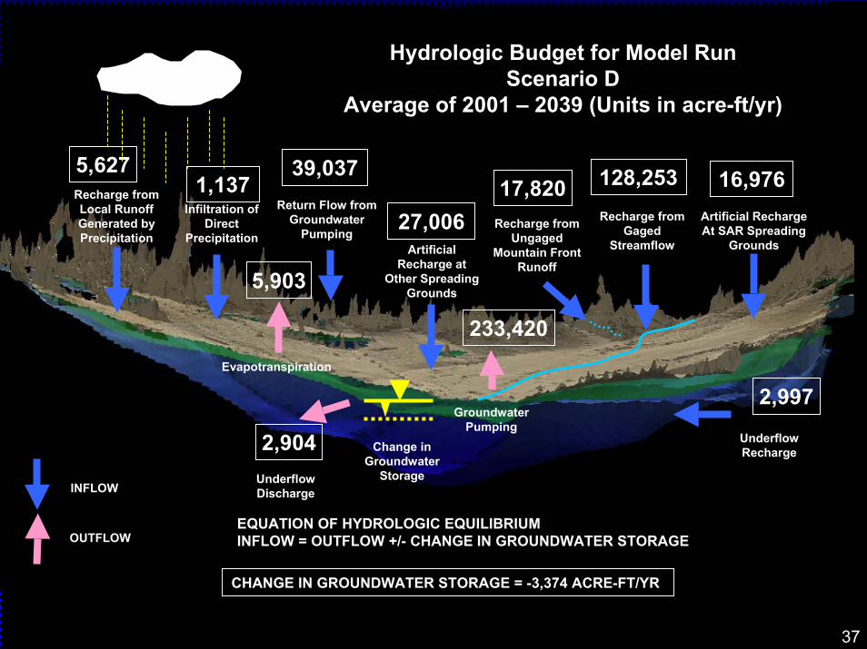
Recharge from Gaged
Streamflow
128,253Infiltration of
Direct Precipitation
1,137Recharge from
Ungaged Mountain Front
Runoff
17,820Recharge from Local Runoff Generated by Precipitation
5,627
Underflow Recharge
2,997
Artificial Recharge at
Other Spreading Grounds
27,006 Artificial Recharge At SAR Spreading
Grounds
16,976Return Flow from
Groundwater Pumping
39,037
Underflow Discharge
2,904
Evapotranspiration
5,903
GroundwaterPumping
233,420
INFLOW
OUTFLOW
Hydrologic Budget for Model Run Scenario D
Average of 2001 – 2039 (Units in acre-ft/yr)
EQUATION OF HYDROLOGIC EQUILIBRIUMINFLOW = OUTFLOW +/- CHANGE IN GROUNDWATER STORAGE
CHANGE IN GROUNDWATER STORAGE = -3,374 ACRE-FT/YR
Change inGroundwater
Storage
37
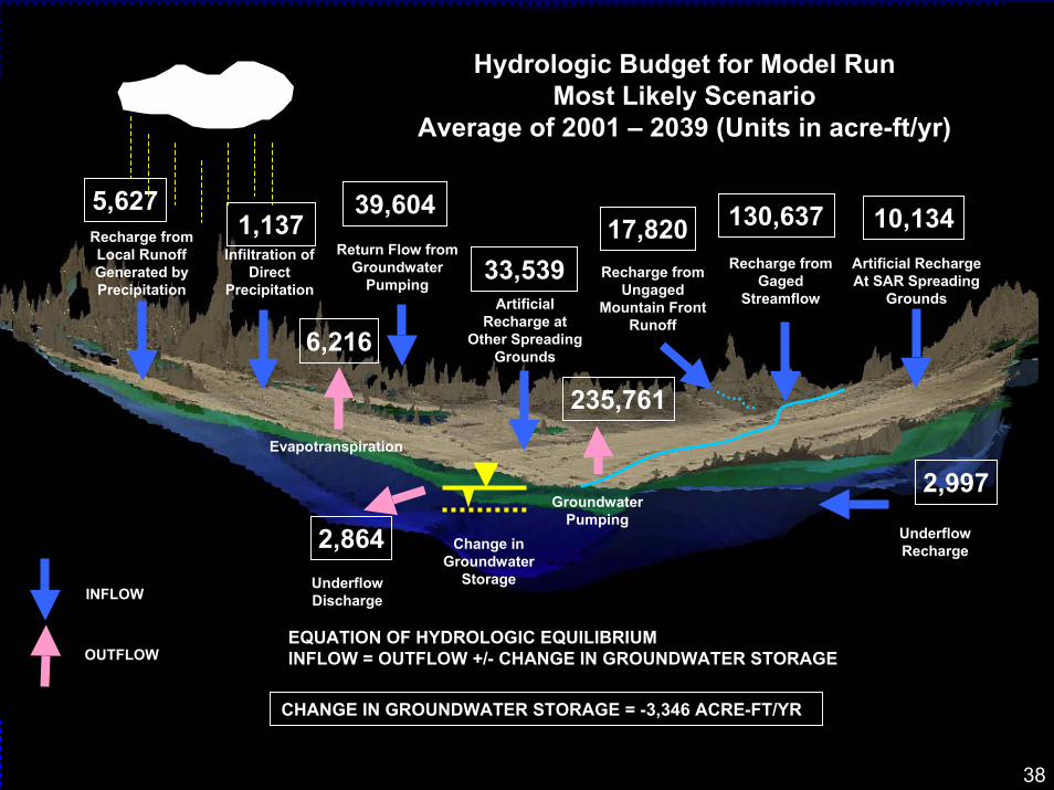
38Muni/Western Ex. 6-389
Recharge from Gaged
Streamflow
130,637Infiltration of
Direct Precipitation
1,137Recharge from
Ungaged Mountain Front
Runoff
17,820Recharge from Local Runoff Generated by Precipitation
5,627
Underflow Recharge
2,997
Artificial Recharge at
Other Spreading Grounds
33,539 Artificial Recharge At SAR Spreading
Grounds
10,134Return Flow from
Groundwater Pumping
39,604
Underflow Discharge
2,864
Evapotranspiration
6,216
GroundwaterPumping
235,761
INFLOW
OUTFLOW
Hydrologic Budget for Model Run Most Likely Scenario
Average of 2001 – 2039 (Units in acre-ft/yr)
EQUATION OF HYDROLOGIC EQUILIBRIUMINFLOW = OUTFLOW +/- CHANGE IN GROUNDWATER STORAGE
CHANGE IN GROUNDWATER STORAGE = -3,346 ACRE-FT/YR
Change inGroundwater
Storage
38

39Muni/Western Ex. 6-389
SBBA Groundwater Budgets 2001-2039SBBA Groundwater Budgets 2001SBBA Groundwater Budgets 2001--20392039
--2222--3,3463,346Most Likely Most Likely ScenarioScenario
--5050--3,3743,374Scenario DScenario D
--8282--3,4063,406Scenario AScenario A
----3,3243,324No ProjectNo Project
Changes as Compared Changes as Compared to No Projectto No Project
[acre[acre--ft/yr]ft/yr]
Change in Groundwater Change in Groundwater StorageStorage
[acre[acre--ft/yr]ft/yr]Model Model
ScenarioScenario
As can be seen, the change in storage under project scenarios are minimal compared to the No Project Condition.
Note: Total groundwater in storage in SBBA is approximately 6 Million Acre-ft (DWR Bulletin 118, 2003)
As can be seen, the change in storage under project scenarios are minimal compared to the No Project Condition.
Note: Total groundwater in storage in SBBA is approximately 6 Million Acre-ft (DWR Bulletin 118, 2003)
40Muni/Western Ex. 6-389
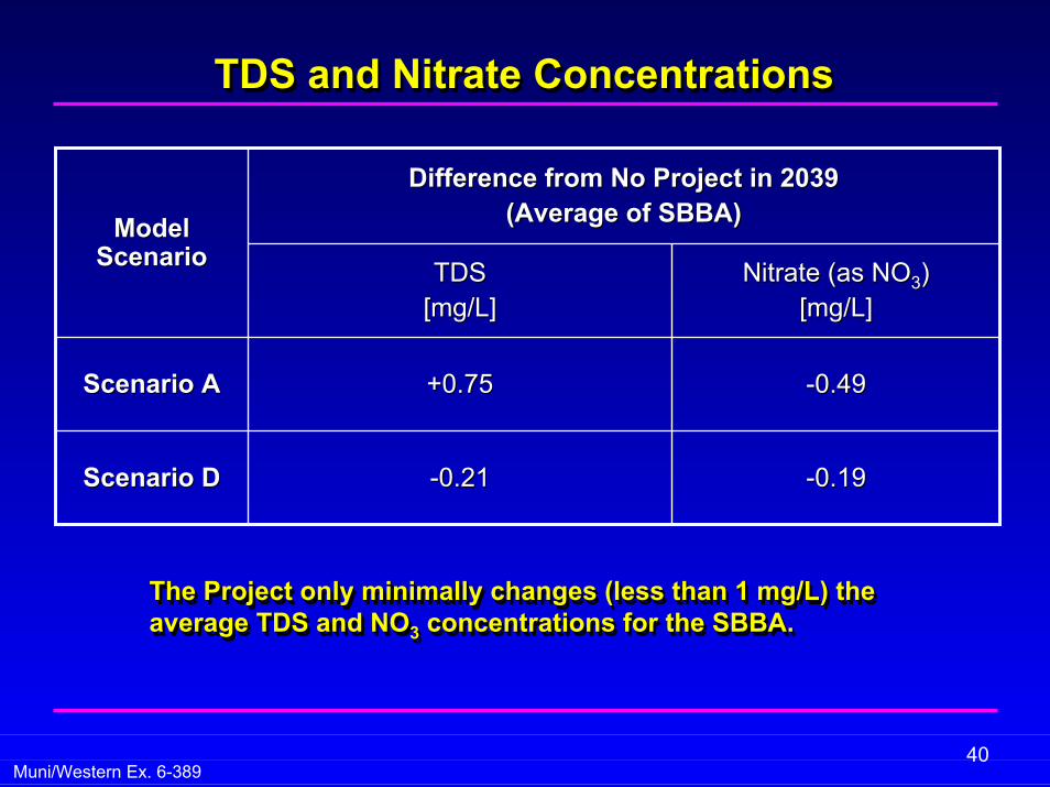
TDS and Nitrate Concentrations TDS and Nitrate Concentrations TDS and Nitrate Concentrations
Nitrate (as NONitrate (as NO33))[mg/L][mg/L]
TDSTDS[mg/L][mg/L]
--0.190.19--0.210.21Scenario DScenario D
--0.490.49+0.75+0.75Scenario AScenario A
Difference from No Project in 2039Difference from No Project in 2039(Average of SBBA)(Average of SBBA)Model Model
ScenarioScenario
The Project only minimally changes (less than 1 mg/L) the average TDS and NO3 concentrations for the SBBA.The Project only minimally changes (less than 1 mg/L) the The Project only minimally changes (less than 1 mg/L) the average TDS and NOaverage TDS and NO33 concentrations for the SBBA.concentrations for the SBBA.

41Muni/Western Ex. 6-389
PCE PlumePCE PlumePCE Plume
No Project Condition Scenario A
20
30 10
039 yrs
Wet
Wet
Wet
Wet
2001-2039 PCE ConcentrationRed: >= 5 ug/LDark Blue: < 5 ug/L

42Muni/Western Ex. 6-389
PCE Plume Areas 2001 -2039
0
500
1,000
1,500
2,000
2,500
3,000
3,500
4,000
4,500
2001 2006 2011 2016 2021 2026 2031 2036
PCE
Plum
e A
rea,
acr
es
No Project
Scenario A
Scenario D
PCE plumes dissipate more rapidly under Project Scenarios compared to No Project. Size of plumes is also smaller under Project Scenarios than under No Project Conditions
43Muni/Western Ex. 6-389
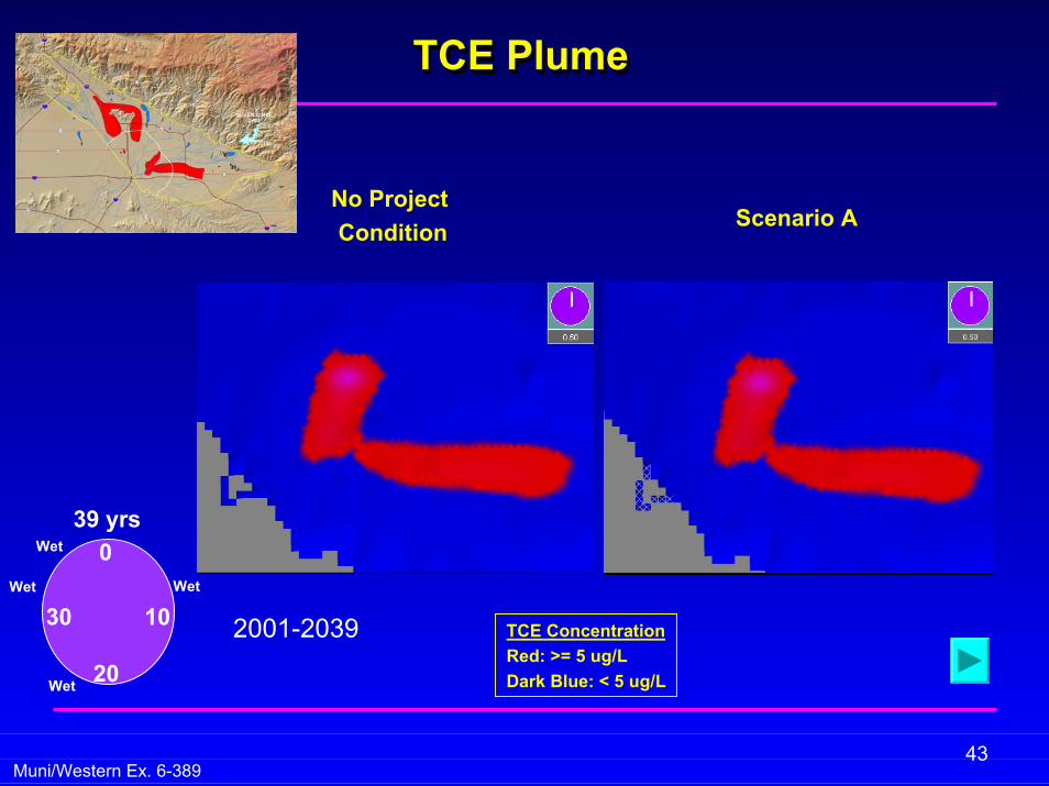
TCE PlumeTCE PlumeTCE Plume
No Project Condition Scenario A
20
30 10
039 yrs
Wet
Wet
Wet
Wet
2001-2039 TCE ConcentrationRed: >= 5 ug/LDark Blue: < 5 ug/L

44Muni/Western Ex. 6-389
TCE Plume Areas 2001 -2039
0
500
1,000
1,500
2,000
2,500
3,000
3,500
4,000
4,500
2001 2006 2011 2016 2021 2026 2031 2036
TCE
Plum
e A
reas
, acr
e
No Project
Scenario A
Scenario D
TCE plumes dissipate more rapidly under Project Scenarios compared to No Project. Size of plumes is also smaller under Project Scenarios than under No Project Conditions
45Muni/Western Ex. 6-389
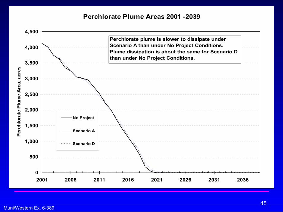
Perchlorate Plume Areas 2001 -2039
0
500
1,000
1,500
2,000
2,500
3,000
3,500
4,000
4,500
2001 2006 2011 2016 2021 2026 2031 2036
Perc
hlor
ate
Plum
e A
rea,
acr
es
No Project
Scenario A
Scenario D
Perchlorate plume is slower to dissipate under Scenario A than under No Project Conditions.Plume dissipation is about the same for Scenario D than under No Project Conditions.

46Muni/Western Ex. 6-389
Overview of Groundwater Models Overview of Groundwater Models Overview of Groundwater Models
♦ Brief Review of Groundwater Modeling Tasks
♦ Results of Groundwater Model Runs
♦ Discussion of Subsidence Modeling
♦ Impacts of Spreading Outside the Model Area
♦♦ Brief Review of Groundwater Modeling TasksBrief Review of Groundwater Modeling Tasks
♦♦ Results of Groundwater Model RunsResults of Groundwater Model Runs
♦♦ Discussion of Subsidence ModelingDiscussion of Subsidence Modeling
♦♦ Impacts of Spreading Outside the Model AreaImpacts of Spreading Outside the Model Area

47Muni/Western Ex. 6-389
Subsidence ModelingSubsidence ModelingSubsidence Modeling
♦ PRESS (Predictions Relating Effective Stress and Subsidence)
♦ Developed by Helm (1975)
♦ Widely Used by Harris-Galveston Coastal Subsidence District
♦ Based on one-dimensional Terzaghi consolidation theory
♦ Input includes changes in water levels from groundwater flow model and properties of compaction layers such as virgin compressibility, elastic compressibility, pre-consolidation stress and thickness of compaction layers
♦ Predicts non-recoverable compaction
♦♦ PRESS (PRESS (PPredictions redictions RRelating elating EEffective ffective SStress and tress and SSubsidence)ubsidence)
♦♦ Developed by Helm (1975)Developed by Helm (1975)
♦♦ Widely Used by HarrisWidely Used by Harris--Galveston Coastal Subsidence DistrictGalveston Coastal Subsidence District
♦♦ Based on oneBased on one--dimensional Terzaghi consolidation theory dimensional Terzaghi consolidation theory
♦♦ Input includes changes in water levels from groundwater flow Input includes changes in water levels from groundwater flow model and properties of compaction layers such as virgin model and properties of compaction layers such as virgin compressibility, elastic compressibility, precompressibility, elastic compressibility, pre--consolidation consolidation stress and thickness of compaction layersstress and thickness of compaction layers
♦♦ Predicts nonPredicts non--recoverable compactionrecoverable compaction

48Muni/Western Ex. 6-389
Subsidence ModelingPRESS Model Calibration Well Raub #8
Subsidence ModelingSubsidence ModelingPRESS Model Calibration Well Raub #8PRESS Model Calibration Well Raub #8
Raub #8
Well Raub #8 was selected because it is located in the Pressure Zone nearest to the maximum historical subsidence and it has geophysical borehole logs.
Well Raub #8 was Well Raub #8 was selected because it is selected because it is located in the Pressure located in the Pressure Zone nearest to the Zone nearest to the maximum historical maximum historical subsidence and it has subsidence and it has geophysical borehole geophysical borehole logs.logs.

49Muni/Western Ex. 6-389
Subsidence at Location of Well Raub #8 (2001-2039)Subsidence at Location of Well Raub #8 (2001Subsidence at Location of Well Raub #8 (2001--2039)2039)
0.01080.01080.430.43Scenario DScenario D
0.01580.01580.620.62Scenario AScenario A
0.00830.00830.350.35No ProjectNo Project
Average Subsidence RateAverage Subsidence Rate[ft/yr][ft/yr]
Total SubsidenceTotal Subsidence[ft][ft]
Model Model ScenarioScenario
The maximum subsidence rate is approximately 1 ft / 100 years for all scenarios. This is within the generally accepted subsidence criteria.The maximum subsidence rate is approximately 1 ft / 100 years for all scenarios. This is within the generally accepted subsidence criteria.

50Muni/Western Ex. 6-389
Overview of Groundwater Models Overview of Groundwater Models Overview of Groundwater Models
♦ Brief Review of Groundwater Modeling Tasks
♦ Results of Groundwater Model Runs
♦ Discussion of Subsidence Modeling
♦ Impacts of Spreading Outside the Model Area
♦♦ Brief Review of Groundwater Modeling TasksBrief Review of Groundwater Modeling Tasks
♦♦ Results of Groundwater Model RunsResults of Groundwater Model Runs
♦♦ Discussion of Subsidence ModelingDiscussion of Subsidence Modeling
♦♦ Impacts of Spreading Outside the Model AreaImpacts of Spreading Outside the Model Area

51Muni/Western Ex. 6-389
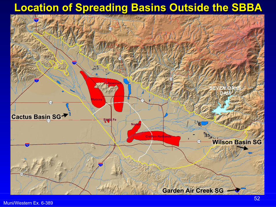
Impacts of Spreading Outside of Model AreaImpacts of Spreading Outside of Model AreaImpacts of Spreading Outside of Model Area
♦ Analytical method used to evaluate impacts of artificial recharge in areas outside of the model area (due to surface spreading)
♦ Hantush Equation which estimates the growth and decay of groundwater mounds in response to uniform percolation
♦ Applied to three artificial recharge areas designated by the Allocation Model :
♦ Cactus Spreading Ground (in Rialto-Colton Basin)
♦ Wilson Spreading Ground (in Yucaipa Basin)
♦ Garden Air Creek Spreading Ground (in San Timoteo Basin)
♦♦ Analytical method used to evaluate impacts of artificial rechargAnalytical method used to evaluate impacts of artificial recharge e in areas outside of the model area (due to surface spreading)in areas outside of the model area (due to surface spreading)
♦♦ Hantush Equation which estimates the growth and decay of Hantush Equation which estimates the growth and decay of groundwater mounds in response to uniform percolationgroundwater mounds in response to uniform percolation
♦♦ Applied to three artificial recharge areas designated by the Applied to three artificial recharge areas designated by the Allocation Model :Allocation Model :
♦♦ Cactus Spreading Ground (in RialtoCactus Spreading Ground (in Rialto--Colton Basin)Colton Basin)
♦♦ Wilson Spreading Ground (in Yucaipa Basin)Wilson Spreading Ground (in Yucaipa Basin)
♦♦ Garden Air Creek Spreading Ground (in San Timoteo Basin)Garden Air Creek Spreading Ground (in San Timoteo Basin)
52Muni/Western Ex. 6-389
Wilson Basin SG
Cactus Basin SG
Muscoy
Newmark
Crafton-Redlands
NortonSanta Fe
Garden Air Creek SG
Location of Spreading Basins Outside the SBBALocation of Spreading Basins Outside the SBBALocation of Spreading Basins Outside the SBBA

Analytical Method Analytical Method –– Hantush EquationHantush Equation
Hantush equation predicts rise and fall of groundwater mounds in response to uniform percolation
53

54Muni/Western Ex. 6-389
Impacts of Spreading Outside of Model AreaImpacts of Spreading Outside of Model AreaImpacts of Spreading Outside of Model Area
13,317 AF13,317 AF45 ft mound45 ft mound
155 ft below land 155 ft below land surfacesurface
Scenario Scenario DD
5,745 AF5,745 AF38 ft mound38 ft mound
122 ft below land 122 ft below land surfacesurface
2,154 AF2,154 AF76 ft mound76 ft mound
74 ft below land 74 ft below land surfacesurface
18,953 AF18,953 AF48 ft mound48 ft mound
152 ft below land 152 ft below land surfacesurface
Scenario Scenario AA
Garden Air Garden Air Spreading GroundsSpreading Grounds(San Timoteo Basin)(San Timoteo Basin)
Wilson Spreading Wilson Spreading GroundGround
(Yucaipa Basin)(Yucaipa Basin)
Cactus Spreading Cactus Spreading GroundGround
(Rialto(Rialto--Colton Basin)Colton Basin)Model Model
ScenarioScenario

55Muni/Western Ex. 6-389
Summary of Comparisons Project Scenarios to No Project – 39 yr Period
Summary of Comparisons Summary of Comparisons Project Scenarios to No Project Project Scenarios to No Project –– 39 yr Period39 yr Period
Minimal Minimal ChangeChange
Minimal Minimal ChangeChange
Minimal Minimal ChangeChange
Change Change in in
Basin Basin StorageStorage
GW Levels GW Levels do not rise do not rise within 50 ft within 50 ft of surfaceof surface
Slightly Slightly More Than More Than
NPNP
Minimal Minimal Change Change
(< 1mg/L)(< 1mg/L)
Dissipates Dissipates Approx the Approx the
SameSame
DissipatesDissipatesMore More
RapidlyRapidly
DissipatesDissipatesMore More
RapidlyRapidly
48% Less 48% Less Than NPThan NP
Scenario DScenario D(Min Cap (Min Cap 500 cfs)500 cfs)
NANA
DissipatesDissipatesMore More
RapidlyRapidly
PCE PCE PlumePlume
NANA
DissipatesDissipatesMore More
RapidlyRapidly
TCE TCE PlumePlume
GW Levels GW Levels do not rise do not rise within 50 ft within 50 ft of surfaceof surface
Slightly Slightly More Than More Than
NPNPNANANANA
67% Less 67% Less Than NPThan NP
Most Likely Most Likely ScenarioScenario(1500 cfs, (1500 cfs, Conserv. Conserv. District District
Settlement Settlement & Senior & Senior
Water Water Rights)Rights)
GW Levels GW Levels do not rise do not rise within 50 ft within 50 ft of surfaceof surface
Impacts of Impacts of Spreading Spreading
Outside Outside SBBASBBA
Slightly Slightly More Than More Than
NPNP
Minimal Minimal Change Change
(<1 mg/L)(<1 mg/L)
Dissipates Dissipates Slightly Slightly SlowerSlower
77% Less 77% Less Than NPThan NP
Scenario AScenario A(Max Cap (Max Cap 1500 cfs)1500 cfs)
Potential Potential SubsidenceSubsidence
Basin Basin Water Water
QualityQuality(TDS (TDS
&NO&NO33))
Perchlorate Perchlorate PlumePlume
Potential Potential LiquefactionLiquefactionScenarioScenario