sar monitoring of progressive and ... - site.tre-altamira.com · ieee transactions on geoscience...

IEEE TRANSACTIONS ON GEOSCIENCE AND REMOTE SENSING, VOL. 41, NO. 7, JULY 2003 1685

SAR Monitoring of Progressive and SeasonalGround Deformation Using thePermanent Scatterers Technique

Carlo Colesanti, Alessandro Ferretti, Fabrizio Novali, Claudio Prati, and Fabio Rocca

Abstract—Spaceborne differential radar interferometry hasproven a remarkable potential for mapping ground deforma-tion phenomena (e.g., urban subsidence, volcano dynamics,coseismic and postseismic displacements along faults, as well asslope instability). However, a full operational capability has notbeen achieved yet due to atmospheric disturbances and phasedecorrelation phenomena. These drawbacks can often be—atleast partially—overcome by carrying out measurements ona subset of image pixels corresponding to natural or artificialstable reflectors [permanent scatterers (PS)] and exploiting longtemporal series of interferometric data. This approach allows oneto push the measurement precision very close to its theoreticallimit (in the order of 1 mm for C-band European RemoteSensing (ERS)-like sensors). In this paper, the detection of bothtime-uniform and seasonal deformation phenomena is addressed,and a first assessment of the precision achievable by means ofthe PS Technique is discussed. Results highlighting deformationphenomena occurring in two test sites in California are reported(Fremont in the Southern Bay Area and San Jose in the SantaClara Valley).

Index Terms—Differential synthetic aperture radar (SAR) inter-ferometry, ground deformation monitoring, permanent scatters.

I. INTRODUCTION

I NTERFEROMETRIC synthetic aperture radar (InSAR) in-volves phase comparison of SAR images, gathered at dif-

ferent times with slightly different looking angles [1]–[4]. It hasthe potential to detect millimetric target displacements along thesensor–target [line of sight (LOS)] direction. Apart from cycleambiguity problems, limitations are due to temporal and geo-metrical decorrelation [5], and to atmospheric artifacts [6]–[11].

Temporal decorrelation makes interferometric measurementsunfeasible where the electromagnetic response of a samplingcell changes with time. Moreover, reflectivity variations as afunction of the incidence angle (i.e., geometrical decorrelation)further limit the number of image pairs suitable for interfero-metric applications, unless this phenomenon is reduced due to

Manuscript received April 1, 2002; revised January 8, 2003. This work wassupported by the European Space Agency European Space Research Instituteunder Contract 13557/99/I-DC.

C. Colesanti, C. Prati, and F. Rocca are with the Dipartimento di Elet-tronica ed Informazione, Politecnico di Milano, 20133 Milan, Italy (e-mail:[email protected]).

A. Ferretti is with the Dipartimento di Elettronica ed Informazione, Politec-nico di Milano, 20133 Milan, Italy and also with the Tele-Rilevamento Europa,T.R.E. S.r.l., 20133 Milano, Italy.

F. Novali is with the Tele-Rilevamento Europa, T.R.E. S.r.l., 20133 Milan,Italy.

Digital Object Identifier 10.1109/TGRS.2003.813278

the pointwise character of the target (e.g., a corner reflector).In areas affected by either kind of decorrelation, reflectivityphase contributions are no longer compensated by generatingthe interferogram [5], and possible phase terms due to targetmotion cannot be highlighted [2]. Finally, atmospheric het-erogeneity superimposes on each SAR image an atmosphericphase screen (APS) that can seriously compromise accuratedeformation monitoring [2], [6]. Indeed, even considering areasslightly affected by decorrelation, it may be extremely difficultto discriminate displacement phase contributions from theatmospheric signature, at least using individual interferograms[2], [6], [12].

In order to reduce the impact of the atmospheric disturbances,interferogram stacking techniques have been outlined [11] anddeveloped [12].

More generally, in order to cope both with atmospheric arti-facts and decorrelation, InSAR approaches aimed at ground de-formation detection are evolving toward the systematic exploita-tion of series of SAR images. Besides permanent scatterers (PS),further techniques are being developed, e.g., [13]–[15].

II. PERMANENT SCATTERERSTECHNIQUE

The PS approach is described in detail in [16] and [17]. Here,we wish to briefly review the core idea, namely the discrimi-nation of the different phase contributions at privileged phase-coherent radar targets exploiting long series of interferometricSAR data like the ones gathered in the European Space Agency(ESA) European Remote Sensing (ERS) archive.

All available images (at least about 25, as we shall see) are fo-cused and coregistered on the sampling grid of a unique masteracquisition, which should be selected keeping as low as possiblethe dispersion of the normal baseline values.

From the available Tandem pairs, a conventional InSAR dig-ital elevation model (DEM) can be reconstructed [1], [18]. Inalternative, an already available DEM can be resampled on themaster image grid.

Given ERS SAR data, differential interferogramscan be generated with respect to the common master acquisition.

Normal baselines values (referred to the orbit of the masterimage) approximately range in the interval m. The tem-poral baseline (with respect to the master acquisition) can ex-ceed five to six years. In order to exploit jointly the whole set ofdifferential interferograms, only phase values relative to point-wise radar targets slightly affected by geometrical decorrelationcan be exploited. Of course, a very reduced impact of temporal

0196-2892/03$17.00 © 2003 IEEE

1686 IEEE TRANSACTIONS ON GEOSCIENCE AND REMOTE SENSING, VOL. 41, NO. 7, JULY 2003

decorrelation is required as well. Privileged radar targets pre-serving phase information under these conditions are hereaftercalled permanent scatterers.

As already described in previous papers [16], [17], the phaseof interferogram gathers four different contributions

- (1)

where 5.66 cm (for ERS data); is the possible targetmotion (with respect to its position at the time of the masteracquisition); is the atmospheric phase contribution;is thedecorrelation noise; and - is the residual topographicphase contribution due to unavoidable errors in the referenceDEM.

The PS approach aims at separating these phase terms by ex-ploiting their different spectral behavior in the framework of amultidimensional [time, space and normal baseline (i.e., acqui-sition geometry)] joint analysis.

• is usually strongly correlated in time and can exhibitdifferent degrees of spatial correlation depending on thephenomenon at hand [17] (e.g., subsidence induced bywater/oil exploitation, creeping along seismic faults, lo-calized sliding areas, instability of individual buildings,etc.).

• shows a strong spatial correlation within every singleSAR acquisition [7]–[10], but is uncorrelated in time.

Even though precise state vectors are available for ERSsatellites [19], the impact of orbit indeterminations cannotbe neglected [17] and induces low-order phase polyno-mials within individual SAR interferograms. Again, thisphase term is strongly correlated in space, but uncorrelatedin time.

Estimated APS is actually the sum of two contributions:atmospheric effects and orbital fringes due to baseline er-rors [17], [20].

• - highlights the exact elevation(hereafter calledDEM error) of the individual radar target (e.g., the roof ofa building) with respect to the reference DEM. -is proportional to the normal baseline and uncorrelated intime.

Neglecting higher order terms, the following simple ex-pression holds [4]:

- (2)

where is the sensor–target distance in correspondenceof the master acquisition ( 845 km in the center of anERS scene); is the local incidence angle ( 23 for flatearth in the center of an ERS scene); andis the height ofthe radar target at hand with respect to the reference DEM.

If the reference DEM is not affected by spatial lowpasserrors, - is practically uncorrelated in space.

Usually this is not the case for interferometric DEMswhere lowpass errors are induced by orbit inaccuraciesand atmospheric effects. - is, therefore, the sumof two contributions, both proportional to the normal base-line and uncorrelated in time, but with different spatialbehavior.

Since at PS an elevation-dependent phase term is esti-mated anyway, it is possible to carry out PS analyses evenwithout using a reference DEM, but simply compensatingthe interferograms for the flat topography phase and re-trieving at PS the entire altimetric phase term, instead ofjust the DEM error contribution. This was performed suc-cessfully even in areas showing steep topographic featureswith height differences exceeding 1000 m.

The description of the processing steps required to isolate thedifferent phase terms and, in particular, to retrieve the atmo-spheric phase contribution is available in [17] and [20].

Here, we just remind informally the basic idea relying ona joint time-normal baseline analysis of the phase differencesrelative to couples of so-called permanent scatterers candidates(PSC) quite close to each other (e.g., within a couple of kilome-ters distance).1 The phase difference is modeled as differentialdeformation and differential topography. Residual terms(gathering differential atmospheric signature and decorre-lation noise ) are expected to have a standard deviation wellbelow (e.g., rad) and can, therefore, be assumed to beunwrapped (in fact, both and are expected showingsmall variations, since the two PSC involved in each differenceare close to each other and are only slightly affected by decor-relation effects). Selecting a PSC as reference and integratingthe in space, unwrapped APS values can be estimated onthe sparse grid of PSC (since noise is spatially uncorrelated, itsimpact is reduced by the integration step). By means of Kriginginterpolation [21], APS data are finally lowpass filtered in space(removal of outliers) and resampled at once on the regular gridof the SAR image.

III. D ETECTION OFGROUND DEFORMATION

Let us assume we have correctly identified the atmosphericphase term (actually APSphase contribution due to orbit in-accuracies). We work, therefore, on differential interferogramscompensated for APS.

The task is now the discrimination of the phase term due toground deformation, from the term due to DEM errors. Theproblem can be solved on a pixel-by-pixel basis (indexes)in a multiinterferogram framework (index)

- (3)

A key issue is the selection of the mathematical model for targetmotion. In the following, two simple models will be addressed.

A. Time-Uniform Deformation

The simplest model we can assume for ground deformation isa constant velocity target displacement, i.e.,(where is the average deformation rate along the sensorLOS, and is the temporal baseline with respect to the masteracquisition). Despite its simplicity, the linear model is extremelyuseful, allowing one to describe many interesting phenomena(e.g., fault creeping, slow evolving subsidence, etc.).

1PSC are points that are likely going to behave as very phase stable PS. Theyare identified by means of a pixel-by-pixel statistical analysis of their amplitudereturns [16] and are a subset of the PS as a whole. The APS estimation step iscarried out on the grid of PSC.

COLESANTI et al.: SAR MONITORING OF PROGRESSIVE AND SEASONAL GROUND DEFORMATION 1687

In this case

(4)

The term gathers both phase decorrelation noiseand possible time-nonuniform deformation.

Since differential interferograms are available, for eachimage pixel we have equations in the unknownsand .

Unfortunately, the phase values are known modulo-2,and, therefore, the system is nonlinear. In fact, even if no defor-mation is occurring, the residual topographic phase will oftenexceed one phase cycle in large baseline interferograms (e.g.,for a 1200-m baseline interferogram, the altitude of ambiguity[3], [4] is around 7.5 m).

The issue can be thought of as a nonlinear inverse problem[22] that can be solved scanning a two-dimensional (2-D)model’s parameter space, seeking the maximum (or the min-imum) of a quality index (or an error function) that has to bechosen.

By defining the single-pixel multiinterferogram complex co-herence (hereafter often simply called coherence) as

(5)

we set as the objective function, maximized bythe couple . Of course, .

This coherence-based approach allows a very interesting in-terpretation of the task as a nonparametric spectral estimationproblem [23].

The coherence operator can be thought of as a 2-D discreteFourier transform of the complex signal (available onan irregular sampling grid) from a domain to adomain.

(6)

The coherence-based estimate corresponds thento the nonparametric estimate of the frequencies of a 2-D com-plex sinusoid, i.e., to the detection of the spectral peak of theperiodogram.

It should be pointed out again that actually the complex signalis irregularly sampled both in time (only slightly, as

we are going to see in a forthcoming section) and normal base-line dimensions.

The higher the multiinterferogram coherence, the more ac-curate and reliable the estimate . Depending on thenumber of available interferograms and on the precision re-quired, we can set a coherence threshold that allows to dis-criminate targets really behaving as permanent scatterers (andwhose LOS deformation can be effectively modeled as time

uniform) from phase-unstable points. Coherence can be inter-preted, therefore, as an“a posteriori” index of the PS behaviorof a radar target, whose reliability depends also on the goodnessof the model chosen for displacement.

As we shall see, the single-pixel multiinterferogram coher-ence allows to infer precious information about the phase sta-bility of the radar target at hand.

If the time series describing the motion of the radar target ismore complex, both time-nonuniform deformation and decor-relation noise contribute to the phase residualsimpacting onthe measured coherence value.

In a forthcoming section we shall discuss the false-detectionprobability, i.e., the probability that a phase-unstable target gen-erates a high value of coherence and is, therefore, misinterpretedas a Permanent Scatterer.

B. Seasonal Deformation

The coherence-based approach can be easily generalized,in order to detect time-nonuniform deformation, by simplyadopting adequate models for the displacement phenomenon tobe investigated [25].

Of course, the problem is still nonlinear, and an increasingnumber of parameters to be estimated makes the computationalburden raising considerably and requires a higher number ofinterferograms to keep reasonably low the risk of overfittingeffects.

In the following we address the detection of seasonal defor-mation phenomena. In particular, we are going to show resultsrelative to the displacement induced by the seasonal depletionand recharge of the groundwater table beneath San Jose (SantaClara Valley, CA) in the area delimited by the Silver Creek andSan Jose seismic faults.

Reversible seasonal ground deformation occurs in all aquifersystems [26]. The relation between a varying groundwater leveland the compression induced on the aquifer system is basedon the principle of effective stress, first proposed by Terzaghi[27]. The principle states that when the support provided by thefluid pressure is reduced (i.e., the groundwater level is lowered)the stress, no longer compensated by the support provided bythe pore-fluid pressure, is transferred to the granular skeletonof the aquitard layers (i.e., the less permeable beds in a strati-graphic sequence), which undergoes progressive compaction.Conversely, when the aquifer system recharges, the stress istransferred back form the fine-grained substaining structure ofthe aquitards to the fluid and the skeleton expands.

The groundwater level usually exhibits seasonal fluctuations,mainlydue to theclimate (e.g.,wetwintersanddrysummers)andto withdrawal of phreatic water, especially for agricultural usageand for supplying large cities and industrial plants. This trans-lates into a completely recoverable deformation occurring in allaquifer systems, resulting in a reversible land surface displace-ment (sometimes even exceeding the amount of 2–3 cm) in re-sponse to the seasonal variation in groundwater pumpage [26].

This kind of seasonal deformation effects have already beenstudied by other authors [e.g., [28], (Los Angeles Basin), [30],(Los Angeles Basin) [31], (San Jose, Santa Clara Valley)].


Often the seasonal behavior is coupled with further phe-nomena, possibly exhibiting a constant displacement rate (e.g.,residual irreversible compaction of an aquifer system [26], ortectonic motion along active seismic faults [30]).

This suggests to assume the following model for grounddisplacement

(7)

The coherence-based inverse problem can be generalized. Themodel space is now four-dimensional. Three dimensions aregiven by the parameters of the model assumed for deforma-tion, namely (amplitude of the seasonal deformation phenom-enon), (temporal offset of the maximum land surface levelwith respect to the date of the master acquisition) and(av-erage deformation rate). As long as we are investigating cyclicphenomena with a 1 year periodicity,is constant ( year).

The same model for displacement is being used in the frame-work of other studies [32], [28].

The fourth parameter is, as usual, the error on the DEM incorrespondence of the scatterer at hand.

The expression, whose absolute value has to be maximized,is now

(8)

Of course, the higher the number of parameters, the higher thecomputational burden and the risk of overfitting effects.

IV. PRECISIONASSESSMENT

As all conventional InSAR products, PS measurements aredifferential both in time and in space. In time, deformation dataare referred to the common master image. In space, data arereferred to a Ground Control Point (GCP) of known position(and, possibly, deformation). We have, therefore, to distinguisha spatial lowpass precision (i.e., a lowpass error, increasing withthe distance from the GCP) and a highpass precision (i.e., thedifferential precision of measurements carried out at individualPS with respect to nearby pixels). We are going to investigatethis second aspect.

The main goal is to extract, from the multiinterferogram co-herence, information about the standard deviationof thephase residuals , and, therefore, about the standard de-viation of individual PS displacement measurements. A secondissue is to evaluate the false PS detection probability, i.e., theprobability that an unstable radar target shows a high value ofcoherence and is therefore interpreted as a PS, due to possibleoverfitting effects.

Furthermore, from , we wish to infer the standard devia-tion of both estimated terms .

A. Statistical Description of and

The first issue is a statistical description of the multiimagesingle-target coherence

(9)

where and are the real and imaginary part of the complexrandom variable .

Let us assume that the phase residualsare uncorrelatedand identically distributed with zero mean and even probabilitydensity function (pdf) . (It is implicitly assumed that themodel adopted for describing surface deformation is adequate;otherwise residuals are no longer uncorrelated. In this case,would underestimate the quality of the corresponding PS mea-surements, as the repeatability can do with global positioningsystem data [29]).

As a consequence of the central limit theorem, bothandare assumed to be distributed as normal random variables.

is, then, a 2-D Gaussian random variable (of course, this is onlyapproximately true, since ).

In order to fully describe , we just need to compute andthe covariance matrix

var covcov var

(10)

It is easy to recognize immediately (since)

(11)

(12)

Moreover

(13)

where is the Fourier transform of the pdf of the phaseresiduals . Since we assumed being an evenfunction

(14)For phase-coherent radar targets, it is reasonable to assume a(zero mean) normal distribution of the residuals induced mainly


by the small amount of decorrelation noise affecting the PS athand

(15)

Starting from the well-known Fourier pair [33],it is easy to prove that

(16)

and, therefore (with the substitution ),.

Finally we get

(17)

Let us evaluate now the elements of the covariance matrixstarting with the variances of and .

For the second-order moment , we obtain

(18)

For (occurring times) we have to compute, for , occurring times .

(19)

The first term can be written as

(20)

where the random variable is still Gaussian with vari-ance . The Fourier transform of the corresponding pdf isthen

(21)

and

(22)

For the other term

(23)

where both random variables andfollow a Gaussian distribution with zero mean and variance

(24)

leading to the following expression:

(25)

In conclusion

(26)

and

(27)

The same steps are repeated to compute

(28)

We notice immediately that , i.e., the complexrandom variable is not circular.

In particular, we obtain

(29)

The covariance is

(30)

and

(31)

Interestingly enough, sine and cosine of the very same symmet-rically distributed (zero mean) random variable are uncorrelated(as a consequence of the fact that covariance can be seen as ascalar product and, therefore, uncorrelation as orthogonality).

is, then, distributed as a 2-D normal random variable withindependent real and imaginary parts, with a real positive av-erage value and with different variances along the two dimen-sions. The pdf depends on the unique parameter: (for thesake of simplicity in the following, we replace and , re-spectively, with and )

(32)

where

(33)

The ratio increases with a decreasingand becomes,therefore, large for PS. With a Mac Laurin expansion we get thefollowing approximation (valid for , i.e., for good PS):

To obtain the marginal distribution for , we transformCartesian coordinates in polar coordinates and in-tegrate along

(34)


Fig. 1. E[j j] and� as a function of� for variousN (number of images available). Errorbars are drawn at�� .

Unfortunately, the integral is not solvable in closed form.For , the expression would lead to a Rice distribu-

tion, but this requires to be close to 1.5 rad, which of coursemeans that we are no longer describing permanent scatterers.

Anyway, having retrieved the is deter-mined as well (even though only numerically) and, startingfrom the measured value for , it is possible to carry outhypothesis testing on to characterize PS more finely.

For the particular issue of describing incoherent radar, it isreasonable to assume uniformly distributed phase values. Thisleads to

(35)

and

(36)

The central limit theorem allows, then, to assume a zero-meancircular Gaussian distribution for

(37)

that transforming Cartesian into polar coordinates andintegrating along leads to a Rayleigh distribution for ofdecorrelating radar targets

(38)

It is worth pointing out that for PS even a simple descriptionof in terms of mean and standard deviation is veryuseful. In fact, since permanent scatterers are characterized bya low phase dispersion of the residues, the measured coherencevalue is very close to . Furthermore, it is rather easyto verify (numerically) that for PS

(39)

thus allowing to estimate directly from the measured

(40)

which can be converted in the dispersion of individualdeformation measurements at single PS

(41)


Fig. 2. �̂ as a function ofN , for significant values ofj ̂j, i.e., 0.7, 0.8, 0.9, 0.95. Uniform temporal sampling is assumed (T = 35-day revisiting time). Sincethe value of̂� depends on the whole observed time span (that for a givenN is going to be larger thanN � T ), the curves plotted are very conservative.

Measured coherence values , and cor-respond to estimated , and mm, respectively.

As already mentioned in the abstract, this very last figure of1 mm can be thought of as an indicative limit for the precisionof C-band ERS-like interferometric measurements. In fact, for ametallic reflector with 1 m area and typical ERS parame-ters ( 0.056 m, area of a sampling cell 80 m ) and as-suming 0 dB (a high value, reasonable for strong clutterin urban areas) we get the following SNR:

SNR (42)

corresponding to a coherence [34]

SNRSNR

(43)

and, therefore, to a 0.9 mm ( 0.19 rad, i.e., around11 ).

As a matter of fact, is deeply related to the conventionalinterferometric coherence defined as

(44)

where and are respectively the master and slave image.is usually computed assuming ergodicity in space and aver-

aging values relative to neighboring pixels of a single interfero-gram after having locally compensated-for deterministic phasecontributions.

Conversely is evaluated on a pixel-by-pixel basis in-volving several interferograms (i.e., somehow along the timedimension).

The main difference is that in the computation of, ampli-tude values are not involved at all. Anyway, for high SNR targets

, and approaches, therefore,the theoretic value of the conventional interferometric coher-ence is

(45)

The estimate can be enriched, providing as well a valuefor the standard deviation of . Again, for PS, the variabilityof depends mainly on the variability of its real part

(46)

In Fig. 1, the estimated values for and are plotted asa function of for various .

Having demonstrated that from a measuredit is possibleto estimate , each PS can be provided with a figure for theprecision of the estimatedand .

In [16], it was already pointed out that, as discussed in [24],the dispersion of a periodogram-based estimate of the spectralpeak of a single tone signal (as long as SNR is high enough)has the same expression of the dispersion relative to a linearregression estimate. In [35] the generalization to the 2-D case isaddressed.

Intuitively this means that as long as the SNR is high enough,phase ambiguity implies nonlinearity of the problem (and, there-fore, requires different solution strategies) but ultimately doesnot affect the precision of the estimate.

Of course, since we are dealing with irregularly sampleddata (in particular, along the normal baseline dimension) thefollowing expressions, directly derived from linear regression


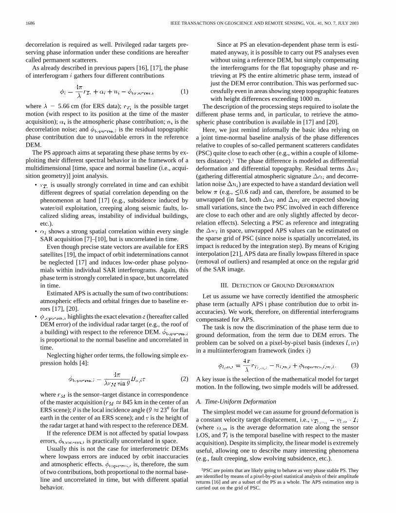
Fig. 3. Relative frequency of occurrence (percentage) of time intervals (k � T wherek = 1; 2; 3; . . .) between successive acquisitions for ERS-1 (A) andERS-2 (B). 487 ERS-1 and 1044 ERS-2 images have been involved in the analysis. Scenes are mainly relative to European and North American test sites, whichare the most regularly covered by ERS acquisitions.

theory [36] and already given in [16], are only approximatelyvalid

(47)

(48)

where and .As a matter of fact, the value measured forat phase stable

PS allows to immediately estimate and, subsequently, and, exploiting the temporal and normal baseline distribution of

the dataset at hand.In Fig. 2, is represented as a function of for significant

values of (hypothesizing regular sampling along time andGaussian distributed normal baseline values. The plausibilityof these assumptions is going to be addressed in a forthcomingsection).

B. False-Detection Probability

We wish now to investigate the false-detection probability,i.e., the probability that an incoherent radar target by chanceshows a high value of and is, therefore, wrongly inter-preted as a PS.

A first coarse evaluation can be performed starting from (38)

(49)

For a finer assessment, we have to take into account the factthat, for discriminating the residual topography phase term fromthe deformation one, we sought for the maximum value of,exploiting the parameters of the model as degrees of freedomand working on wrapped phase data.

We have to look for the distribution of the following randomvariable

(50)

where is a candidate set of parameters (and are tem-poral and normal baseline vectors).

Unfortunately, since we are exploring the parameter spacewith a fine sampling step, the quantities cannotbe considered independent. The problem gets rather difficult,and its analytical solution is not trivial.

For a rapid assessment of the false PS detection probability,it is, therefore, more convenient to run numerical simulations,involving the distribution of ERS acquisitions along time andnormal baseline while exploring the model’s parameter space.

1) ERS Data Sampling Along Time and Baseline Dimen-sions: A first assessment of the distribution of ERS dataspacing along time and normal baseline has been carried out,exploiting orbital data relative to a considerable amount of ERSacquisitions that have been involved in PS analyses carried outat Polimi and Tele-Rilevamento Europa—T.R.E. S.r.l (a Polimispin-off company).

A total of 1531 scenes (487 ERS-1 and 1044 ERS-2) acquiredin the Northern Hemisphere (approximately between latitudes30 N and 65 N) over Europe, North Africa, Asia, and NorthAmerica, in the time span 1992–2000, have been used to retrievea sampled pdf of the ERS data as a function of time and normalbaseline (2001 data have been discarded, since after the failureof gyro 1 on January 7, 2001, ERS-2 operations have been per-formed in Extra Backup Mode (EBM) with orbit deadband re-quirements lowered from 1 km to 5 km, [37]).

The results are well summarized in Figs. 3–5.

The following conclusions can be drawn.

• As a first approximation, ERS data (in particular ERS-2data) can be assumed being regularly spaced in time, sincethe time span between successive acquisitions amounts tothe 35-day revisiting time with an occurrence of 73% and56% (respectively, ERS-2 and ERS-1; see Fig. 3).

• On the other hand, the normal baseline distribution ismore complex and quite different for the two sensors. Tomake comparable baseline values relative to acquisitionsbelonging to different scenes (and, therefore, not part of ahomogeneous dataset referred to a unique master) meanvalues have been discarded.


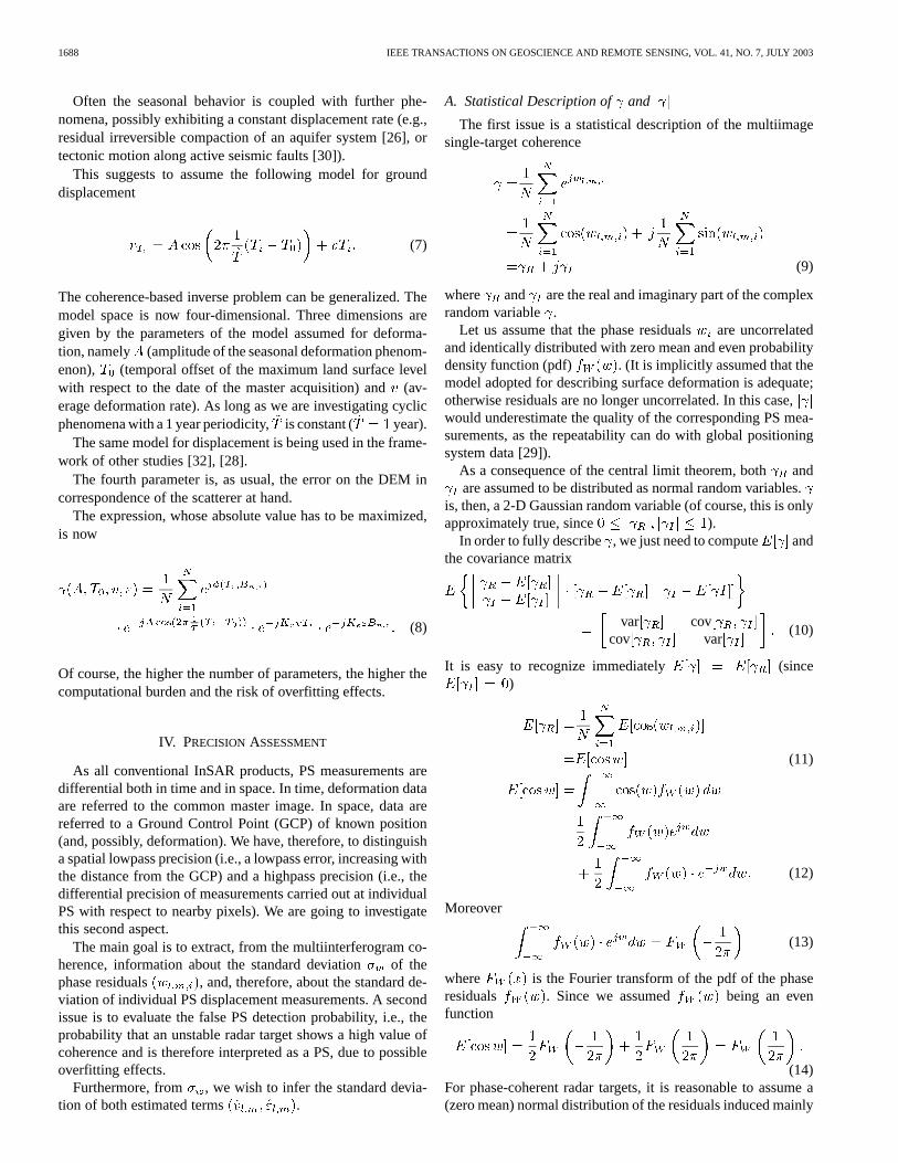
Fig. 4. Histograms displaying the occurrence of normal baseline values in (A) ERS-1 (487 scenes involved) and (B) ERS-2 (1044 scenes involved) acquisitions.

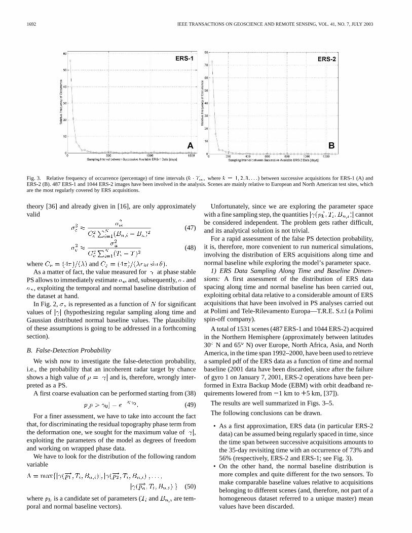
Fig. 5. Joint ERS-1/2 sampled normal baseline pdf (rhombs). For the purpose of a qualitative description, a Gaussian fitting (� = 0; � = 482 m) matchessatisfactory the sampled pdf.

The ERS-2 normal baseline distribution can be roughlyapproximated with a zero-mean triangular-shaped function.The sampled standard deviation amounts to around 465 m (seeFig. 4).

ERS-1 data, conversely, show a more articulated behavior,being quite uniform in the interval 600 m and then exhibitingasymmetric tails. The sampled standard deviation is a bit larger,about 515 m (see Fig. 5).

The histogram (and, therefore, the sampled pdf function)could be approximated with a generalized Gaussian [22], eventhough this does not take account of the skewness.

The physical interpretation of both sampled pdfs is still inprogress.

Separate analyses relative to ascending and descendingpasses have been carried out as well, but did not highlight anysignificant difference with respect to the joint one.

The ERS-1/2 combined sampled pdf is depicted inFig. 5. A simple, but very effective approximation is to assumea Gaussian behavior with zero mean and standard deviation482 m.

2) Numerical Simulations:In order to estimate precisely thefalse PS detection probability, numerical simulations havebeen carried out, generating uniformly distributed random phasevalues, carrying out the joint periodogram-based estimateand retrieving the measured value of .


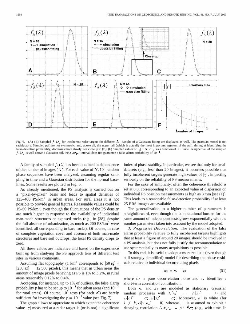
Fig. 6. (A)–(E) Sampledf (�) for incoherent radar targets for differentN . Results of a Gaussian fitting are displayed as well. The guassian model is notsatisfactory. Sampled pdf are not symmetric, and, above all, the upper tail (which is actually the most important segment of the pdf, aiming at identifying thefalse-detection probability) decreases more slowly; see closeup in (B). (F) Sampled values ofj j � 3:3� as a function ofN . Since the upper tail of the sampledf (�) is well above a Gaussian tail, the3:3� interval does not guarantee a false-alarm probability of 10.

A family of sampled has been obtained in dependenceof the number of images . For each value of 10 randomphase sequences have been analyzed, assuming regular sam-pling in time and a Gaussian distribution for the normal base-lines. Some results are plotted in Fig. 6.

As already mentioned, the PS analysis is carried out ona “pixel-by-pixel” basis and leads to spatial densities of125–400 PS/km in urban areas. For rural areas it is notpossible to provide general figures. Reasonable values could be15–50 PS/km, even though the fluctuations of the PS densityare much higher in response to the availability of individualman-made structures or exposed rocks (e.g., in [38], despitethe full absence of urbanization, as much as 200 PS/kmwereidentified, all corresponding to bare rocks). Of course, in caseof complete vegetation cover and absence of both man-madestructures and bare soil outcrops, the local PS density drops tozero.

All these values are indicative and based on the experiencebuilt up from studying the PS approach tens of different testsites in various continents.

Assuming flat topography (1 kmcorresponds to50 rg250 az 12 500 pixels), this means that in urban areas theamount of image pixels behaving as PS is 1% to 3.2%, in ruralareas reasonably 0.12% to 0.4%.

Accepting, for instance, up to 1% of outliers, the false alarmprobability has to be set up to 10 for urban areas (and 10for rural areas). Of course, 10tests (for each ) are barelysufficient for investigating the 10 value (see Fig. 7).

The graph allows to appreciate to which extent the coherencevalue measured at a radar target is (or is not) a significant

index of phase stability. In particular, we see that only for smalldatasets (e.g., less than 20 images), it becomes possible thatfully incoherent targets generate high values of, impactingseriously on the reliability of PS measurements.

For the sake of simplicity, often the coherence threshold isset at 0.8, corresponding to an expected value of dispersion onindividual PS position measurements as high as 3 mm [see (1)].This leads to a reasonable false-detection probability if at least25 ERS images are available.

The generalization to a higher number of parameters isstraightforward, even though the computational burden for thesame amount of independent tests grows exponentially with thenumber parameters taken into account by the model adopted.

3) Progressive Decorrelation:The evaluation of the falsealarm probability relative to fully incoherent targets highlightsthat at least a figure of around 20 images should be involved ina PS analysis, but does not fully justify the recommendation touse systematically as many acquisitions as possible.

To this end, it is useful to adopt a more realistic (even thoughstill strongly simplified) model for describing the phase resid-uals relative to individual decorrelating pixels

(51)

where is pure decorrelation noise and identifies ashort-term correlation contribution.

Both and are modeled as stationary Gaussianrandom processes with and

. Moreover, is white (for), whereas is assumed to exhibit a

decaying correlation (e.g., with time. In


Fig. 7. Threshold on sampled coherence (as a function ofN ) for having a false-alarm probabilityp � 10 . The estimate obtained from (49) (Rayleighdistribution for j j) has been computed assuming to use justN � 2 phase values to take into account two degrees of freedom (corresponding to the modelparameters: velocity and DEM error). As mentioned in the text, the agreement is only qualitative, even though still useful for a low number of images. Themaximum value of sampled coherence obtained in 10tests is plotted as well.

principle, the same behavior could be envisaged with respectto the normal baseline as well, even though in this latter caseirregular data sampling should be taken into account). Finally,

and are, of course, mutually uncorrelated.The variance of the residuals identifies the phase

stability of the radar target at hand, and can be estimated as

(52)

Conversely, the variance of ( ) identifies the pre-cision of the phase stability estimate relative to the target and is,therefore, an index that can be used to quantify the false-detec-tion probability.

can be computed directly from its definition

(53)

It is very easy to show that

(54)

The computation of

(55)

is slightly more cumbersome, even though conceptuallystraightforward. Involving the correlation model assumedfor , remembering that for a zero-mean Gaussian randomvariable , , neglecting terms, and assuming

is large enough to approximate partial sums of geometricsuccessions with the corresponding series, we obtain

(56)

leading to following expression for the variance of:

(57)

gathering the effects of both decorrelation noise and short-termcoherence contributions.

If we assume that the residuals are due to pure decorrelationnoise we get

(58)

Conversely, if we assume that the only contribution is due toshort-term coherence we get

(59)

highlighting, that as a consequence of the correlation in theresiduals, the variance of the estimate of the phase dispersiondecreases more slowly, as a function of an equivalent number ofimages

(60)


(e.g., for , for andfor ).

This shows that, for discriminating PS from short-term co-herent targets, a higher number of images is required. Of course,if is high, these latter radar targets provide useful interfero-metric information and deserve being examined in a suitablesubdataset. Anyway, considering them as full PS rises the risk ofdrawing wrong conclusions and introducing false alarms (e.g.,outliers in a displacement time series).

V. RESULTS

The major advantages of the PS approach are a remarkableprecision coupled with a high spatial density of benchmarks.A further interesting property is the availability of point dis-placement data, enabling to describe motion affecting individualstructures.

On the other hand, the main limit is related to the intrinsicambiguity of phase measurements that prevents the techniquefrom being able to monitor rapidly evolving deformation phe-nomena [25] (the theoretical limit given by the sampling the-orem is 14 mm/35 days and can be circumvented only if it ispossible to model and exploit the spatial correlation of the dis-placement phenomenon at hand).

Moreover, a sufficient spatial PS density (5–10 PS/km) isrequired to properly estimate and remove atmospheric artifacts,and at least about 25 images are necessary to fulfill a reliable PSanalysis.

In order to highlight and prove the advantageous properties ofthe technique, we wish to show some significant results relativeto two test sites in California, namely Fremont in the SouthernBay Area and San Jose at the northwestern end of the SantaClara Valley.

Forty-six ERS-1/2 images gathered along descending or-bits in the time span May 1992–November 2000 have beenexploited.

The reference point deformation data both test sites are rel-ative to was chosen in Fremont, between the Gomes Park andthe Mission San Jose Community Park, a couple of kilometersnorth of the area represented in Fig. 8 (noa priori was availableto confirm whether the reference point is really motionless).

A. Progressive Time-Uniform Deformation

As already mentioned, the model for time-uniform deforma-tion is often sufficient for properly describing creeping alongactive seismic faults. In particular, attention has been devoted tothe Southern Hayward Fault, identifying by means of the PS ap-proach the average deformation rate (along the ERS LOS) gra-dient crossing the fault.

The Hayward Fault is part of the San Andreas Fault Systemand crosses the densely populated East Bay Area. As a matterof fact, the 1868 7.0-magnitude earthquake [39] that beforethe 1906 event used to be referred to as the “great San Fran-cisco earthquake” occurred on the Hayward Fault. Often, twosegments are distinguished, namely the Northern and SouthernHayward Fault [40]. The northern segment has been studied in-tensively by means of traditional interferometry [41], [42]. We

will focus on the Southern Hayward Fault extending approxi-mately from (37.45N, 121.81 E), around 15 km NE of SanJose, to (37.73N, 122.13 E), beneath San Leandro, with alength of about 43 km [40]. The Hayward Fault is a right-lateralstrike-slip fault. An estimated value for the slip rate is9 mm/year [40], [43]. Other studies [44] based on high-preci-sion deformation data recorded at creepmeters provide a similarfigure for the slip rate at Fremont ( 8.5 1 mm/year,Osgood road, in the time span 1993–1997) highlighting that to-ward north (Hayward, Palisdes road) the slip rate decreases to

0.05 mm/year (in the same time span).Precision and (temporal) sampling frequency of creepmeter

displacement data are extremely high (respectively a small frac-tion of a millimeter and up to 10-min temporal sampling interval[44]).

As already mentioned, SAR interferometry allows to detectdeformation along the target-sensor LOS, which can be identi-fied by means of a normalized vector (often referred to as sensi-tivity vector [2], [20], since it summarizes the system sensitivityto ground displacement).

In Fremont, the sensitivity versor exhibits the followingcomponents:

(61)

can be assumed constant over areas of several square kilome-ters, since it varies slowly, mainly as a function of the incidenceangle (i.e., of the range coordinate of the pixel at hand).

The fault trace trends S 48.8E ( 41.2 with respect toEasting; see Fig. 8), and since horizontal creeping is occurringwe can project the slip rate along Easting and Northingobtaining

mm/yearmm/year

mm/year(62)

The velocity variation along the ERS LOS can be obtained as

scalar product .The figure mm/year detected at the creep-

meter along Osgood Road is translated in mm/year,which matches pretty well the sharp gradient in LOS velocitymeasured at PS crossing the Hayward Fault along section AA’(approximately 3.2 mm/year), i.e., along Carol Avenue, within afew hundreds of meters from the creepmeter. In Fig. 8, the LOSvelocity of the PS closest to section AA’ is depicted. It should bepointed out that these velocity values have been retrieved at in-dividual radar targets, without interferogram filtering (Kriginginterpolation of the APS values estimated on the sparse gridof permanent scatterers Candidates is, of course, a spatial low-pass filtering operation. However, since from the interferometricphase of single radar targets a spatially correlated term (the esti-mated APS) is removed, the final effect resembles more a high-pass filtering step, even though, of course, deformation termsthat are correlated both in time and space are left unchanged).

PS displayed in Fig. 8 show , leading therefore to0.67 rad and 3 mm (on each measurement of the

relative position of single PS). Since .


Fig. 8. Fremont, Southern Hayward Fault. (I) Position and average LOS displacement rate of PS(j j > 0:8) represented on a high radiometric quality multiimagereflectivity map. The image is in SAR coordinates and covers an area of about 5.5� 2.8 km . Direction and versus of tectonic slip are highlighted. (II) AverageLOS deformation rates of individual PS along section AA’. The LOS velocity of the PS nearest to the section is plotted. The 3.2-mm/year step in the LOS averagedisplacement rate matches well the LOS projection of a figure of 8.5 mm/year (creepmeter data) for horizontal slip. (III) LOS deformation time seriesof PSmarked 1. in (I) The 2.5-mm step in the time span November 1995–May 1996 matches well the sudden deformation recorded at the creepmeter (Osgood road).Other high-coherence PS in the immediate neighborhood highlight the same small step.


Fig. 9. Seasonal surface deformation in San Jose. The area undergoing seasonal displacement is delimited by the Silver Creek and San Jose Fault. (A) AmplitudeA and (B) temporal offsetT of the sinusoidal model fitting the motion of each PS are represented on a geocoded multiimage reflectivity map (area imaged:18� 11 km ). (C)–(H) High accuracy localization on aerial photography and time series relative to two permanent scatterers (I.) and (II.) on opposite sides of theSilver Creek Fault.

Finally, given the temporal sampling of the ERS data available,we obtain 0.2 mm/year. The PS spatial density amountsto around 170 PS/km. Section AA’ is about 3.5 km long. Theaverage deformation rate of PS along the section highlights thatbesides the velocity discontinuity in correspondence of the fault,on the western side of the rupture (i.e., toward A’), a smoothgradient in the displacement rate can be appreciated within thefirst several hundred meters (one azimuth pixel corresponds to4 m) from the fault.

Moreover, creepmeter data [44] highlight a sudden dis-placement of 5 mm during February 1996 (about 7 mm in thetime span 30 November 1995-1 May 1996). Projected alongthe ERS LOS, this last figure is translated in 2.35 mm. In thedisplacement time series of the very best permanent scatterers

in the immediate neighborhood (within 2 km),something similar seems to occur. For instance, Fig. 8 depicts

the time series of a PS located at the crossroad WashingtonBoulevard–Castillajo Way (1 km from the creepmeter).Unfortunately, no ERS records are available in the time spanDecember 1995–April 1996. Between the Tandem pairs of19 951 110–19 951 111 and 19 960 503–19 960 504, a small stepof 2.5 mm seems to have occurred (measured as the defor-mation between average position relative to each Tandem pair).

and, therefore, 1.15 mm. (Since we arecomputing the difference of two independent measurements,this figure should increase, but this latter effect is compensatedby the averaging of the two position records relative to eachTandem pair.) Of course, such a millimetric deformation isvery close to the theoretical limit of PS measurement precision,not allowing to claim with certitude the correct detection ofthe rapid millimetric slip occurring along the fault in February1996 (also because of the lack of ERS data immediately before


and after the phenomenon). Nevertheless, we point out thatother PS in the immediate neighborhood show similar trends.

Moreover, a vertical slip of the same magnitude would bedetected without problem, since its projection along the ERSLOS is much larger.

B. Seasonal Deformation

Further interesting results have been obtained studying thearea of San Jose at the northwestern end of the Santa ClaraValley, where the zone delimited by the Silver Creek and the SanJose Fault undergoes strong seasonal deformation. As alreadymentioned in a previous section, we are facing the reversiblecompaction and dilation of the aquifer system in response to aseasonally fluctuating groundwater level [31].

Adopting the simple sinusoidal model for seasonal deforma-tion introduced in a previous section, very interesting resultshave been obtained.

Estimated amplitude and temporal offset for each individualPS are represented in Fig. 9. The area affected bysignificant seasonal displacement is sharply delimited by theSilver Creek Fault. As expected, motion occurs coherently, andall radar targets move synchronously (see Fig. 9). The PS den-sity is rather high; setting the coherence threshold at 0.8, it ex-ceeds the amount of 230 PS/km. The peak-to-peak amplitude(i.e., ) of the oscillation achieves 3 cm, in agreement withwhat has been highlighted by other studies [46] and measured atborehole extensometers in San Jose [45]. The sensitivity versorrelative to downtown San Jose is slightly different from the onerelative to Fremont

(63)

Again, SAR data take account only of the deformation oc-curring along the LOS direction (the combination of ascendingand descending data allows to solve for two directions). Underthe hypothesis that the whole deformation occurring takes placealong the vertical direction, ERS deformation data could berescaled with the factor to match vertical dis-placement data, even though the correction is often below thetheoretical limit on the system sensitivity (1 mm).

The sharp gradient in the amplitude of the seasonal deforma-tion across the Silver Creek Fault (Fig. 9) deserves being studiedfrom a geological and geophysical point of view in order to inferinformation relative to the permeability of the first stratigraphiclayers crossed by the rupture. More generally, further investiga-tions should be devoted to analyzing displacement phenomenaalong the Silver Creek Fault, a Quaternary fault considered tec-tonically inactive [45] but poorly known (right lateral strike slipcharacter, traditionalin situ geological survey did not allow toestimate the slip rate and assess whether some activity is stilloccurring or not [48]).

On the other side, the gradient across the San Jose Fault ismuch more gentle, suggesting a higher permeability and com-pressibility of the surface layers. (The San Jose Fault is charac-terized by a low slip rate, 0.5 mm/year [40].)

As a significant example, the position of a PS on the crossroadU.S. Route 101 and Zanker Road, in proximity of the San Jose

International Airport, has been mapped on high-resolution aerialphotography [47]. The corresponding deformation time series isdepicted in Fig. 9, showing a peak-to-peak excursion of about2 cm . Position and time series of a further PS, northof the Silver Creek Fault are given as well (Fig. 9). The PS corre-sponds to the building on the crossroad Murphy Avenue–LundyAvenue and is not affected by deformation . The dis-tance between the two radar targets amounts to around 2 km.

VI. CONCLUSION

The PS technique is a fully operational powerful tool allowingto exploit long series of interferometric SAR data aiming athigh-precision ground deformation mapping. We showed bothanalytically and experimentally that the precision of the tech-nique achieves values of 1–3 mm on individual measurementsand 0.1–0.5 mm/year on the average deformation rate. More-over, since PS are pointwise targets whose elevation is knownwith high precision as well (1 m [16]), deformation data canbe mapped on the corresponding structures (e.g., in a geographicinformation system environment or using either aerial photog-raphy or high-resolution spaceborne optical imagery).

The precision assessment of the technique deserves furtherstudies, in particular to investigate the spatial lowpass error in-creasing with the distance from the ground control point PS re-sults are relative to.

A further research issue is the combination of PS data rela-tive to adjacent tracks and ascending and descending passes inorder to increase the PS spatial density and to cross-validate re-sults [49], as well as to map deformation along two independentdimensions.

ACKNOWLEDGMENT

ERS-1 and ERS-2 SAR data were provided by ESA-ESRIN.The support of ESA and particularly of L. Marelli, M. Doherty,B. Rosich, and F. M. Seifert is gratefully acknowledged. Theauthors are thankful to R. Bürgmann for helpful discussions.Finally we would like to thank R. Locatelli, M. Basilico, andA. Menegaz, who developed most of the processing softwarewe used, as well as the whole Tele-Rilevamento Europa staff.

REFERENCES

[1] A. K. Gabriel, R. M. Goldstein, and H. A. Zebker, “Mapping small el-evation changes over large areas: Differential radar interferometry,”J.Geophys. Res., vol. 94, 1989.

[2] D. Massonnet and K. L. Feigl, “Radar interferometry and its applicationto changes in the earth’s surface,”Rev. Geophys., vol. 36, 1998.

[3] P. A. Rosen, S. Hensley, I. R. Joughin, F. K. Li, S. N. Madsen, E. Ro-driguez, and R. M. Goldstein, “Synthetic aperture radar interferometry,”Proc. IEEE, vol. 88, pp. 333–382, Mar. 2000.

[4] R. Bamler and P. Hartl, “Synthetic aperture radar interferometry,”Inv.Prob., vol. R1, 1998.

[5] H. A. Zebker and J. Villasenor, “Decorrelation in interferometric radarechoes,”IEEE Trans. Geosci. Remote Sensing, vol. 30, pp. 950–959,Sept. 1992.

[6] D. Massonnet and K. L. Feigl, “Discrimination of geophysical phe-nomena in satellite radar interferograms,”Geophys. Res. Lett., vol. 22,1995.

[7] R. F. Hanssen, “Atmospheric heterogeneities in ERS tandem SAR inter-ferometry,” Delft Univ. Press, Delft, The Netherlands, DEOS Rep. 98.1,1998.

[8] , Radar Interferometry. Data Interpretation and Error Analysis,Dordrecht, The Netherlands: Kluwer, 2001.


[9] S. Williams, Y. Bock, and P. Pang, “Integrated satellite interferometry:Tropospheric noise, GPS estimates and implications for interferometricsynthetic aperture radar products,”J. Geophys. Res., vol. 103, 1998.

[10] R. M. Goldstein, “Atmopsheric limitations to repeat-track radar inter-ferometry,”Geophys. Res. Lett., vol. 22, 1995.

[11] H. A. Zebker, P. A. Rosen, and S. Hensley, “Atmospheric effects in inter-ferometric synthetic aperture radar surface deformation and topographicmaps,”J. Geophys. Res., vol. 102, 1997.

[12] D. T. Sandwell and E. J. Price, “Phase gradient approach to stackinginterferograms,”J. Geophys. Res., vol. 103, 1998.

[13] S. Usai, “A new approach for long term monitoring of deformations bydifferential SAR interferometry,” Ph.D. Thesis, Delft Univ. Technology,Delft, The Netherlands, 2001.

[14] P. Berardino, G. Fornaro, A. Fusco, D. Galluzzo, R. Lanari, E. Sansosti,and S. Usai, “A new approach for analyzing the temporal evolution ofearth surface deformations based on the combination of DIFSAR inter-ferograms,”Proc. IGARSS, 2001.

[15] M. Costantini, F. Malvarosa, F. Minati, L. Pietranera, and G. Milillo, “Athree-dimensional phase unwrapping algorithm for processing of multi-temporal SAR interferometric measurements,”Proc. IGARSS, 2002.

[16] A. Ferretti, C. Prati, and F. Rocca, “Permanent scatterers in SAR inter-ferometry,”IEEE Trans. Geosci. Remote Sensing, vol. 39, pp. 8–20, Jan.2001.

[17] , “Nonlinear subsidence rate estimation using permanent scatterersin differential SAR interferometry,”IEEE Trans. Geosci. RemoteSensing, vol. 38, pp. 2202–2212, Sept. 2000.

[18] , “Multibaseline InSAR DEM reconstruction: The wavelet ap-proach,” IEEE Trans. Geosci. Remote Sensing, vol. 37, pp. 705–715,Mar. 1999.

[19] R. Scharroo and P. Visser, “Precise orbit determination and gravity fieldimprovement for the ERS satellites,”J. Geophys. Res., vol. 103, 1998.

[20] C. Colesanti, A. Ferretti, C. Prati, and F. Rocca, “Monitoring landslidesand tectonic motion with the permanent scatterers technique,”Eng.Geol., vol. 68, no. 1–2, pp. 3–14, Feb. 2003.

[21] H. Wackernagel,Multivariate Geostatistics, 2nd ed, Berlin, Germany:Springer-Verlag, 1998.

[22] A. Tarantola,Inverse Problem Theory, Methods for Data Fitting andModel Parameter Estimation. Amsterdam, The Netherlands: Elsevier,1987.

[23] S. L. Marple, Digital Spectral Analysis with Applications. UpperSaddle River, NJ: Prentice-Hall, 1987.

[24] D. C. Rife and R. R. Boorstyn, “Single-tone parameter estimation fromdiscrete-time observations,”IEEE Trans. Inform. Theory, vol. IT-20,1974.

[25] C. Colesanti, F. Novali, and R. Locatelli, “Ground deformation moni-toring by means of SAR permanent scatterers,”Proc. IGARSS, 2002.

[26] D. Galloway, D. R. Jones, and S. E. Ingebritsen, Eds., “Land Subsidencein the United States,” U.S. Geolog. Surv., Reston, VA, Circular 1182,1999.

[27] K. Terzaghi, “Principles of soil mechanics, IV—Settlement and consol-idation of clay,”Eng. News-Rec., vol. 95, no. 3, 1925.

[28] K. M. Watson, Y. Bock, and D. T. Sandwell, “Satellite interferometricobservations of displacements associated with seasonal ground water inthe Los Angeles Basin,”J. Geophys. Res., to be published.

[29] J. Zhanget al., “Southern california permanent GPS geodetic array:Error analysis of daily positions estimates and site velocities,”J. Geo-phys. Res., vol. 102, no. B8, 1997.

[30] G. W. Bawden, W. Thatcher, R. S. Stein, K. W. Hudnut, and G. Peltzer,“Tectonic contraction across Los Angeles after removal of groundwaterpumping effects,”Nature, vol. 412, 2001.

[31] R. Bürgmann, private communication, 2001.[32] B. M. Kampes, R. F. Hanssen, and L. M. Th. Swart, “Strategies for

nonlinear deformation estimation from interferometric stacks,”Proc.IGARSS, 2001.

[33] S. Haykin, An Introduction to Analog and Digital Communica-tions. New York: Wiley, 1989.

[34] C. Prati and F. Rocca, “Range resolution enhancement with multipleSAR surveys combination,”Proc. IGARSS, 1992.

[35] P. Pasquali, “Generazione di mappe altimetriche con interferometriaSAR,” Ph.D. Thesis, Politecnico di Milano, Milan, Italy, 1994.

[36] H. L. Larsen,Introduction to Probability Theory and Statistical Infer-ence, 2nd ed. New York: Wiley, 1974.

[37] Earth Observation, Earthnet Online, All News Archive “ERS-2 opera-tions status” (2001, Feb. 8). [Online]. Available: http://earth.esa.int/cgi-bin/news_archive?2001

[38] J. F. Dehls, M. Basilico, and C. Colesanti, “Ground deformation moni-toring in the ranafjord area of norway by means of the permanent scat-terers technique,”Proc. IGARSS, 2002.

[39] USGS Earthquake Hazards Program—Northern California: HaywardFault Subsystem: 1868 earthquake, USGS. [Online]. Available:http://quake.wr.usgs.gov/prepare/ncep/hayward.html

[40] Fault table, T. Barnhard and S. Hanson. (1996). [Online]. Available:http://geohazards.cr.usgs.gov/eq/faults/fault_table.pdf

[41] R. Bürgmann, E. Fielding, and J. Sukhatme, “Slip along the Haywardfault, California, estimated from space-based synthetic aperture radarinterferometry,”Geology, vol. 26, no. 6, 1998.

[42] R. Bürgmann, D. Schmidt, R. M. Nadeau, M. d’Alessio, E. Fielding,D. Manaker, T. V. McEvilly, and M. H. Murray, “Earthquake potentialalong the northern Hayward Fault, California,”Science, vol. 289, 2000.

[43] Working Group on Northern California Earthquake Potential, “Databaseof potential sources for earthquakes larger than magnitude 6 in NorthernCalifornia,” U.S. Geolog. Survey, Reston, VA, Open-File Rep. 96-705,1996.

[44] R. Bilham. Earthquakes and tectonic plate motions. Univ. Colorado,Boulder, CO. [Online]. Available: http://cires.colorado.edu/~bilham/

[45] M. E. Ikehara, D. J. Galloway, E. Fielding, R. Bürgmann, S. Lewis, andB. Ahmadi, “InSAR imagery reveals seasonal and longer-term land sur-face elevation changes influenced by ground-water levels and fault align-ment in Santa Clara Valley, California,”EOS Trans. AGU, vol. 79, no.45, p. 37, 1998.

[46] D. L. Galloway. Measuring land subsidence from space. [Online]. Avail-able: http://water.wr.usgs.gov/rep/fs05100/insar2.pdf

[47] Aerial photography [Online]. Available: http://www.mapquest.com/maps

[48] Northeast San Jose Transmission Reinforcement Project. CaliforniaPublic Utilities Commission. [Online]. Available: http://www.cpuc.ca.gov/divisions/energy/environmental/info/aspen/ nesanjo/secC/C-5.pdf

[49] C. Colesanti, A. Ferretti, C. Prati, and F. Rocca, “Full exploitation ofthe ERS archive: Multi data set permanent scatterers analysis,”Proc.IGARSS, 2002.

Carlo Colesanti was born in Milan, Italy, in 1974.He received the “Dottore in Ingegneria delle Telco-municazioni” degree from the Politecnico di Milano,Milan, Italy, in 1999. He is currently pursuing thePh.D. degree at the Politecnico di Milano.

His main research interest is in the field of syn-thetic aperture radar. He has been working since 1999on the permanent scatterers technique and on the de-velopment of a passive SAR system reusing the signaltransmitted by television broadcasting satellites.

Mr. Colesanti received the “Premio ENEA per loSviluppo Sostenibile”award in 1999 and the Symposium Prize Paper Award atIGARSS’99.

Alessandro Ferretti was born in Milan, Italy, onJanuary 27, 1968. He received the “laurea” degreein electrical engineering from Politecnico di Milano(POLIMI), Milan, Italy, in 1993, the “master” degreein information technology from the Educationand Research Center in Information Technology,Politecnico di Milano (CEFRIEL), Milan, Italy,working on digital audio compression, and the Ph.D.degree in electrical engineering from POLIMI, in1997.

In May 1994, he joined the POLIMI SAR group,working on SAR interferometry and digital elevation model reconstruction. Hevisited the Department of Geomatic Engineering (formerly Photogrammetryand Surveying), University College London, London, U.K., during the summerof 1996. His Ph.D. thesis topic addressed the use of multibaseline SAR interfer-ograms for more reliable phase-unwrapping algorithms. His research interestsconcern digital signal processing and remote sensing. He is currently ManagingDirector of Tele-Rilevamento Europa-TRE, Milan, Italy. He is coinventor of thepatent on the permanent scatterers technique.


Fabrizio Novali received the “laurea” degree(summa cum laude) in electronic engineeringfrom the Politecnico di Milano (POLIMI), Milan,Italy, in 2000, studying techniques to estimate andremove atmospheric artefacts in differential SARinterferometry.

He joined Tele-Rilevamento Europa, Milan, Italy,working on the permanent scatterers technique anddevoting his activity to development and implemen-tation of algorithms and software. His main researchinterests are the retrieval of atmospheric phase con-

tributions and of time-nonuniform deformation effects in multiimage SAR in-terferometry exploiting the PS approach.

Claudio Prati was born in Milan, Italy, on March 20,1958. He received the Ph.D. degree from the Politec-nico di Milano (POLIMI), Milan, Italy, in 1987.

From 1987 to 1991, he was with the Centro StudiTelecomunicazioni Spaziali of the Italian NationalResearch Council, Ispra, Italy. He was a VisitingScholar with the Department of Geophysics, Stan-ford University, Stanford, CA, during the autumnof 1987. He became an Associate Professor ofsystems for remote sensing at POLIMI in 1991. Heis currently a Full Professor of telecommunications.

He has been responsible for the SAR interferometry experiments at the RemoteSensing Lab of the Joint Research Centre of the European Commission (JRC),Ispra, Italy. He holds three patents on SAR image processing. He publishedmore than 80 papers.

Dr. Prati is a Member of the “FRINGES” (ESA) group, of the Committeeon Earth Observation Satellites (CEOS). He was awarded two prizes from theIEEE Geoscience and Remote Sensing Society (IGARSS’89 and IGARSS’99).

Fabio Rocca received the Dottore degree (cumlaude) in ingegneria elettronica from the Politecnicodi Milano (POLIMI), Milan, Italy, in 1962.

He has been with the Department of ElectronicEngineering, POLIMI, since 1962, first as a TeachingAssistant, then as Associate Professor, and thenProfessor of radiotechniques first and now digitalsignal processing. He visited the System SciencesDepartment, University of California, Los Angeles,from 1967 to 1968, and then the Department ofGeophysics, Stanford University, Stanford, CA,

from 1978 to 1979, 1981, 1983, and 1986. His research work has been devotedto digital signal processing for television, reflection seismology, biomedicine,and synthetic aperture radar.

Dr. Rocca was Chairman of the Department of Electronic Engineering,POLIMI, from 1975 to 1978 and then on the University Board (Commissioned’Ateneo, 1980–1993). He was President of the Osservatorio GeofisicoSperimentale, a National Institute for Research in Geophysics, from 1983 to1984. He is a Member of the Scientific Council of the Institut Francais duPetrole, and of the Italian Space Agency (ASI). He is an Associate Editor ofthe journalsSignal ProcessingandSeismic Exploration. He is Past Presidentof the European Association of Exploration Geophysicists. He received theIEEE Geoscience and Remote Sensing Society Symposium Prize Paper awardin 1989 and 1999.

sar monitoring of progressive and ... - site.tre-altamira.com · ieee transactions on geoscience...

Documents