sar sea-ice image analysis based on iterative region ...dclausi/papers/published 2007/yu and...

IEEE TRANSACTIONS ON GEOSCIENCE AND REMOTE SENSING, VOL. 45, NO. 12, DECEMBER 2007 3919

SAR Sea-Ice Image Analysis Based on IterativeRegion Growing Using Semantics

Qiyao Yu and David A. Clausi, Senior Member, IEEE

Abstract—Synthetic aperture radar (SAR) has been intensivelyused for sea-ice monitoring in polar regions. A computer-assistedanalysis of SAR sea-ice imagery is extremely difficult due tonumerous imaging parameters and environmental factors. Thispaper presents a system which, with some limited informationprovided, is able to perform an automated segmentation andclassification for the SAR sea-ice imagery. In the system, both thesegmentation and classification processes are based on a Markovrandom-field theory and are formulated in a joint manner un-der the Bayesian framework. Solutions to the formulation areobtained by a region-growing technique which keeps refining thesegmentation and producing semantic class labels at the same timein an iterative manner. The algorithm is a general-segmentationapproach named iterative region growing using semantics, which,in this paper, is dedicated to the problem of classifying the opera-tional SAR sea-ice imagery provided by the Canadian Ice Service(CIS). The classified image results have been validated by the CISpersonnel, and the resulting classifications are quite successfulusing the same algorithm applied to diverse data sets.

Index Terms—Expert system, image segmentation, Markov ran-dom field (MRF), region growing, sea ice, synthetic apertureradar (SAR).

I. INTRODUCTION

SYNTHETIC aperture radar (SAR) has been intensivelyused for sea-ice monitoring in polar regions and has been

found to have important applications in both scientific and oper-ational activities such as climatic research and ship navigation.In the Canadian Ice Service (CIS), daily ice charts are pro-duced based primarily on RADARSAT-1 SAR sea-ice images.Other sources for producing daily ice charts include ERS-2,NOAA_AVHRR, SSM/I & OLS, QuikSCAT, and previous-dayice charts. Ice charts are sent to coast guards and merchant shipsfor route planning in sea-ice-infested regions. In producing anice chart, ice analysts decompose the image into polygon re-gions, with each polygon representing a visually homogeneousarea in the SAR image. A symbol called the egg code, definedby the World Meteorology Organization (WMO) [1], is thenassigned to each polygon region, summarizing the informationabout the type, concentration, and floe size of each ice typeexisting inside the region. Operationally, this analysis is done

Manuscript received December 14, 2006; revised June 9, 2007. This workwas supported in part by the Natural Sciences and Engineering Research CenterNetwork of Centres of Excellence (NCE) called Geomatics for Informed Deci-sions (GEOIDE), by the Canadian Ice Service (CIS), and by the CRYosphericSYStem (CRYSYS) in Canada.

Q. Yu is with Eutrovision Inc., Shanghai 200030, China (e-mail:[email protected]).

D. A. Clausi is with the Department of Systems Design Engineering,University of Waterloo, Waterloo, ON N2L 3G1, Canada (e-mail: [email protected]).

Digital Object Identifier 10.1109/TGRS.2007.908876

manually, and it is limited in throughput, has human bias, anddoes not classify at a pixel-level resolution.

Computer-assisted analysis is thus desired, the goal of whichis to properly segment the image into homogeneous regions andto classify each segmented region with the correct ice type inan automated manner. This will generate an ice map whereeach pixel is assigned a particular ice type. Unfortunately,significant variations exist with respect to the tone (intensity)and texture appearance of the SAR sea ice due to the complexityof environmental factors and the backscattering and interactionof electromagnetic radiation with the sea ice. Moreover, the ex-istence of notorious speckle noise adds considerable difficultyin extracting the real tone and texture features of the SAR seaice. The task is thus extremely challenging with respect to bothsegmentation and classification.

The success of a SAR sea-ice analysis system is thus largelydependent upon its adaptivity to the variable tones and texturesof the SAR sea ice. On the other hand, models that are relativelyinsensitive to the tones and textures are needed for robustdescriptions of the ice types. The two issues are associatedwith the two processes, respectively: the low-level unsupervisedsegmentation on image pixels and the high-level supervisedclassification on segmented regions. In the latter, features otherthan the tone and texture need to be efficiently incorporated, assuggested by the success of human operators in discriminatingthe ice types using additional high-level knowledge such asfloe shape and existence of fractures. Computing such featuresrequires the low-level segmentation to produce correct regionsneither oversegmented nor undersegmented. Such a balance isdifficult to achieve due to the complexity of the sea-ice scenes,and hence, guidance by the high-level supervised classificationis desirable for the low-level-segmentation process.

Such a bidirectional relationship between the segmentationand classification has not been explored before in the SAR sea-ice field. Except for a number of supervised studies [2]–[7]that directly assign each pixel with an ice-type label, mostexisting publications [8]–[11] deal only with the segmentationtask without considering further classification of the segmentedregions. As such, the features utilized in all those methods arelimited to tone and texture. Some systems [12]–[15] have in-tegrated a classification process but in a postprocessing mannerthat does not allow the segmentation process to benefit from theincorporation of various high-level features in the classificationprocess.

This paper aims at designing a computer-based analysissystem in support of the CIS operations. The system, withthe egg code provided, performs an automated joint segmen-tation and classification of the corresponding polygon regionin RADARSAT-1 sea-ice images. Both the segmentation andclassification processes in the system are based on the Markov

0196-2892/$25.00 © 2007 IEEE

3920 IEEE TRANSACTIONS ON GEOSCIENCE AND REMOTE SENSING, VOL. 45, NO. 12, DECEMBER 2007

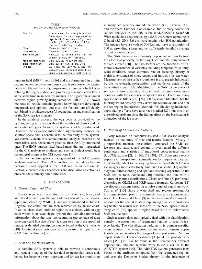
TABLE IICE CATEGORIES DEFINED BY WMO [1]

random-field (MRF) theory [16] and are formulated in a jointmanner under the Bayesian framework. A solution to the formu-lation is obtained by a region-growing technique which keepsrefining the segmentation and producing semantic class labelsat the same time in an iterative manner. The algorithm is namediterative region growing using semantics (IRGS) [17]. Novelmethods to include domain-specific knowledge are developed,integrated, and applied, and also, the features are efficientlycombined to produce successful segmentation and classificationof the SAR sea-ice imagery.

In the analysis process, the egg code is provided to thesystem, giving information about the number of classes and theassociated ice types. As such, the system is not fully automated.However, the egg-code information significantly reduces thesolution space and is beneficial to the reliability of the system.We currently deem this semiautomated analysis process to bemore robust and, hence, more practical than the fully automatedones. The IRGS outputs pixel-based maps that are impracticalfor the CIS analysts to produce, and such a product would be ameaningful progress for CIS operations [14].

The next section gives a background of the SAR sea-iceanalysis research. The IRGS method is then described inSection III and applied to the SAR sea ice in Section IV.Section V presents the experiments and discussions. Section VIpresents the summary and future work.

II. BACKGROUND

A. Sea-Ice Types and Chart

Sea ice is generally a mixture of freshwater ice, brine, andair. Based primarily on the age and thickness of the ice, sea-icetypes are defined by WMO [1] and are summarized in Table I.Regional ice conditions are then represented by an ice chart.In an ice chart, each outlined region is associated with an eggcode which is an oval-shape symbol that contains numericalinformation about the type, concentration (percentage of areacoverage), and floe size of each ice type existing in the specifiedregion. A detailed description can be found at the CIS website[18]. Digitized ice charts have also been used as input to theSAR classification in [19].

B. SAR Sea-Ice Backscatters

A satellite SAR system is able to provide a continuousand regular imaging of the ice-field-overextended areas and,hence, has become a very important tool for sea-ice monitoring

in many ice services around the world (i.e., Canada, U.S.,and Northern Europe). For example, the primary source forsea-ice analysis in the CIS is the RADARSAT-1 ScanSARWide mode data acquired using a SAR instrument operating atC-band (5.3-GHz 5.6-cm wavelength) with HH polarization.The images have a swath of 500 km and have a resolution of100 m, providing a large and yet sufficiently detailed coverageof vast ocean expanses.

The SAR backscatter is mainly dependent on two factors:the electrical property of the target ice and the roughness ofthe ice surface [20]. The two factors are the functions of nu-merous environmental variables including temperature, salinity,wind condition, ocean currents, rate of freezing, history ofmelting, existence of snow cover, and intrusion of sea water.Measurement of the surface roughness is also greatly influencedby the wavelength, polarization, and incidence angle of thetransmitted signal [21]. Modeling of the SAR backscatters ofsea ice is thus extremely difficult and becomes even morecomplex with the existence of speckle noise. There are manyspeckle-noise filters [22]–[26] in the research literature, but thefiltering would possibly break down the texture details and blurthe ice-region boundaries. Methods for alleviating incidence-angle fading effects have also been studied [27], but this is anunresolved problem since the fading effect on the backscatter isa function of the ice type.

C. Review of SAR Sea-Ice Analysis

Early research on computer-assisted SAR sea-ice analysisfocused on the study of tone and texture features. Mostly ina supervised manner, these efforts compared the SAR sea-ice tone and texture, and generally investigated the differentparameters and statistics of gray-level cooccurrence matrix(GLCM) textures [2], [3], [6], [7], [28], [29]. Some more recentpapers use unsupervised segmentation techniques as they cantheoretically adapt to the varying backscatters of the SAR sea-ice imagery more effectively. Soh and Tsatsoulis [11] applieda dynamic-thresholding and spatial-clustering algorithm to theSAR sea-ice tone. Samadani [10] modeled the tone with amixture of gamma distributions. Clausi and Yue [8] performedclustering on GLCM and MRF texture features. Karvonen [12]developed a system based on a pulse-coupled neural network.Soh et al. [15] chose a watershed and region growing forthe segmentation part of a complete analysis system namedARKTOS. Deng and Clausi [9] implemented an MRF model toaccount for the spatial relationship among pixels for producingsegmentation results less sensitive to the SAR speckle noise.Yang et al. [30] applied a region-based MRF to polarimetricSAR sea-ice data.

Such research does not typically deal with the classification,namely, the assignment of segmented regions to specific ice-type labels. The classification task, as it is domain-specific,often requires the integration of numerous domain expertknowledge and involves the design of an expert system. Variousexpert systems, knowledge-based [31]–[34] or probabilistic-based [35], [36], can be found in the literature for differentapplications, and one relevant work to SAR sea ice is theARKTOS system [15]. The ARKTOS system generates factsbased on the attributes computed from the segmented regionsand uses the Dempster–Shafter theory for the inference of

YU AND CLAUSI: SAR SEA-ICE IMAGE ANALYSIS BASED ON ITERATIVE REGION GROWING 3921

facts. The map-guided MAGSIC [14] is another SAR sea-ice classification system, which accumulates evidence for icetyping by exploring a correlated information between the egg-code regions in the ice chart. MAGSIC uses [9] to segment eachpolygon SAR region.

III. ITERATIVE REGION GROWING

USING SEMANTICS (IRGS)

Traditionally, the segmentation and classification (if any) areperformed separately, with the classification as a postprocessingof the segmentation. A substantial deficiency of such a simpleunidirectional link between the two processes is the fact that thesegmented regions may not match the real objects well enoughfor an accurate subsequent classification. In fact, segmentationis generally not a stand-alone problem, but ill-posed if notassociated with some constraints, which can be defined from animplicit or explicit interpretation (classification). Therefore, theclassification needs to be able to guide the segmentation, andhence, a bidirectional relationship between the two is desired.

The applied method here is called the IRGS and is basedon [17]. A more extensive description of the segmentation-only component is presented in a chapter by Yu [37]. Themethod is characterized by a gradually increased edge penalty(with the difference of penalty between weak and strong edgesbeing gradually reduced) in the objective function and a region-growing segmentation controllable by a labeling process. Weextend such a general-segmentation method to the SAR sea-ice analysis by integrating a SAR sea-ice specific classificationinto the labeling process and by building a bidirectional rela-tionship between segmentation and classification. The systemthus allows the segmentation to benefit from the incorporationof various high-level features, such as the shape of ice floes andexistence of fractures, which have been important in the oper-ational human analysis of SAR sea-ice images. In this section,the segmentation component is described, and in Section IV,the classification, as it pertains to the SAR sea-ice imagery, isalso described.

A. Markov Random Field (MRF)

The MRF [16] provides a method of modeling the jointprobability distribution of the image sites in terms of localspatial interactions. In an MRF, each site s ∈ S is related toothers via a neighborhood system ηs. A random field X is anMRF on S with respect to the neighborhood system ηs if andonly if

P (X = x) > 0 ∀x ∈ XP (xs|xS−ηs

) =P (xs|xηs) (1)

where X is the configuration space of random field X. By theHammersley–Clifford theorem [38]

P (X=x)=1Z

exp −E(x)=1Z

exp

−

∑c∈C

Vc(x)

(2)

where C is the set of cliques which are defined as the sets ofmutually neighboring sites, Vc(x) is the energy of configuration

x on clique c, E(x) is the total energy of configuration x, and Zis the normalizing constant. The clique-energy functions modelthe interactions among pixels in a neighborhood. By definingdifferent forms of clique-energy functions, various MRFs aredesigned.

The image-segmentation task can be formulated as amaximum a posteriori problem in which maximizing thea posteriori P (x|y) gives a solution. Here, y = ys|s ∈ Srepresents all pixel values on the image lattice S, and x =xs|s ∈ S represents the class labels on S. By the Bayes’ rule,this is equivalent to maximizing p(y|x)P (x) in which the priorP (x) is typically modeled by an MRF [9], [16], [39], [40] toincorporate a spatial-context information. For this purpose, amultilevel logistic (MLL) model has been popular [39] whoseclique energy is defined as

V (xs, xt) =β, if xs = xt

0, otherwise(3)

where s and t are the neighboring sites forming a pair-siteclique, and β is a positive number. With such a model, the priorP (x) is large if a local neighborhood region is dominated byone single class and small, otherwise.

Based on the assumption that the value ys of each pixel s is aconstant gray level (related to the corresponding class label xs)corrupted by an additive independent noise, a Gaussian featuremodel can be used to give an analytical expression of p(y|x).The formulation of the segmentation task then becomes

X = arg minxs,s∈S

∑s∈S

12

ln(2πσ2

xs

)+

(ys − µxs)2

2σ2xs

+β∑

〈s,t〉∈C1 − δ(xs − xt)

(4)

where µxsand σ2

xsare the mean and variance of all pixel values

in class xs, and δ(·) is the Kronecker delta function.

B. Incorporating Edge Strength

The traditional MRF segmentation model is initiated byassuming that each pixel has a random label assigned to it.Here, a region adjacency graph (RAG) is employed [16] tosave computation time to assist proper initialization that helpsto lead to a globally optimal solution and because regionstatistics are less sensitive to outliers. A watershed algorithm[41] is run to generate a preliminary oversegmented system,and the RAG is built using the watershed result. Each node inthe RAG represents a region (an independent spatial groupingof pixels), and each link represents the common boundarybetween the regions. The edge strength between for each ad-jacent region pair is used in the segmentation and classificationapproaches.

Applying a greater penalty to weak edge and a lesser penaltyto strong edge is possible instead of penalizing equally for allboundary-site pairs as in (4). With a penalty function defined as

g(∇st) = g (|ys − yt|) = e−(|ys−yt|/K)2 (5)


the IRGS method uses a sequence of objective functions in (6)(with K increasing) to approach to the segmentation formula-tion of (4) from the standard Gaussian mixture problem

X = arg minxs,s∈S

∑s∈S

12

ln(2πσ2

xs

)+

(ys − µxs)2

2σ2xs

+β∑

〈s,t〉∈C(1 − δ(xs − xt)) g(∇st)

. (6)

The IRGS segmentation is an iterative process. At eachiteration, the solution to the objective function (6) for a givenK is obtained by a region-merging process and a region-basedlabeling. The merging criterion is [17]

δE =∑s∈Ωk

ln(σk) −∑s∈Ωi

ln(σi) −∑s∈Ωj

ln(σj)

−β∑

s∈∂Ωit∈∂Ωj ,t∈ηs

g (|yt − ys|) (7)

where Ωi and Ωj are the two regions, Ωk = Ωi

⋃Ωj , and ∂Ωi

is the set of boundary sites of Ωi (i.e., ∃t ∈ ηs, xs = xt). If δEgives a negative value, Ωi and Ωj can be merged, and if δEproduces a positive value, Ωi and Ωj will not be merged. Whenthe region-merging process is completed (i.e., no remainingregion pairs satisfy the merging criterion), a RAG [16] canbe updated from the obtained regions. An MRF based on theRAG is used to model the region-based labeling process, andthe corresponding single-node clique-energy function is

V1(xi) =∑s∈Ωi

12

ln(2πσ2

xi

)+

(ys − µxi)2

2σ2xi

(8)

and the pair-node clique energy is

V2(xi, xj)=β

∑s∈∂Ωi

t∈∂Ωj ,t∈ηs

g (|yt − ys|) , if xi =xj

0, otherwise(9)

where xi is the label of region Ωi. Finding the global minimumof the summation of the above energies over the entire RAG,which is exactly (6), gives a labeling for the current iteration. Agreedy combinatorial optimization process is applied.

C. IRGS Algorithm

The overall algorithm of IRGS is described in Table II. Atfirst, an initial RAG is built based on a deliberately overseg-mented result [41]. Random labels are then assigned to eachnode, and the iterative process begins with the feature-modelparameter estimation based on the current labeling. Region-merging and labeling processes are then performed duringeach iteration, and when completed, a new iteration beginswith an increased edge penalty. The iterations continue untila maximum number of iterations1 have been reached. It shouldbe noted that the two regions Ωi and Ωj are not allowed to be

1We set it to 100, and our experiments all converge (no further configurationchanges of x) within 80 iterations.

TABLE IIALGORITHM OF THE GENERAL IRGS SEGMENTATION

merged if they do not have the same label, the purpose of whichis to suppress the merging between parts of different objects thathave weak boundaries in between. This concept is known assemantic region growing [42], [43], and similar ideas also exist[44]. Here, the merging and labeling are iterative and, as such, isreferred to as IRGS. Although the labeling process modeled by(8) and (9) has no semantic meanings, it is possible to replaceit with a domain-specific labeling process and to integrate high-level knowledge. This is presented in the next section.

IV. IRGS APPLIED TO SAR SEA-ICE IMAGERY

For the classification of SAR sea ice, the domain knowledgeincludes tone (intensity), texture, shape, and existence of frac-tures. Thicker ice generally has brighter tones than thinner icetypes within the same image, but such a tendency is not reliabledue to the influence of factors such as snow cover, surfaceroughness, and incidence variations.

Texture has the potential to be relatively insensitive to inci-dence variations and has attracted most of the attention inthe SAR sea-ice community. Two kinds of textures, microtex-ture and macrotexture, are possible for ice identification. Anexample is shown in Fig. 2(a). Here, the water and land areasare found predominantly in the bottom middle of the scene.Regions that are relatively dark, containing brighter lines (iceridges caused by pressure), are gray–white ice, and the restof the regions represent gray ice. The gray ice has noticeablecoarser microtextures, whereas the gray–white ice is character-ized by macrotextures formed by dark floes and bright ridges.However, microtextures are often masked by speckle noise,and macrotextures are heavily scale-dependent. Descriptive(with respect to ice types) and reliable features are difficult toextract for both kinds of textures. In this paper, texture is notconsidered.

A more robust feature used extensively by ice analysts isthe floe shape. Thicker ice typically has well-defined ellipticalfloes. For example, as shown in Fig. 4(a), it is dominatedby two ice types (medium first year and thick first year).The thick first-year ice, although thicker than the other, isrelatively dark. The identification of thick first-year ice thuscannot be based on the tone feature but on the existence of well-defined floes.


Existence of fractures is another possible feature. Although itis not definite that the occurrence of fractures indicates thinnerice types, thin ice types such as gray and gray–white are oftenobserved to have leads (long narrow fractures that ships cannavigate through). In Fig. 2(a), dominant leads are clearlyvisible in the thinner gray-ice region.

In this section, the above domain-specific knowledge is in-corporated in the labeling steps of the IRGS process also bymeans of clique-energy functions. In addition to the general-segmentation clique functions (8) and (9), new clique functionsare designed to give decreased values if the correspondingclassification of the regions tends to be consistent with themeasurements and domain knowledge [35].

A. Tone

The simplest unary property of a segmented region is themean of the tone. However, tone is sensitive to environmen-tal factors and imaging parameters. The SAR backscatter forvarious ice types has high intraclass variance, making distinc-tion based on the absolute backscatter not possible. We havenoticed, however, that there is more useful information basedon the relative difference of tone rather than the absolute value,and hence, this information is more appropriately representedby a pair-node clique function rather than a single-node clique-energy function. The negative logarithm of the distributionof the tone difference is a reasonable choice for the form ofthe corresponding clique-energy function. However, this re-quires extensive training which is limited by the availability ofground truth data. A much simpler clique function is used here,namely

V(td)2 (xi, xj)

=

LijC

(td), xi is thicker ice, y(td)i < y

(td)j

LijC(td), xj is thicker ice, y(td)

i > y(td)j

0, otherwise

(10)

where y(td)i is the mean tone of region Ωi, and C(td) is a

positive number experimentally set. Lij is the length of theboundary between regions Ωi and Ωj and is included in thisclique-energy function based on the intuition that the impor-tance of a binary relation between two neighboring regionsshould be related to their common boundary length. Therefore,all pair-node clique-energy functions are weighted by this com-mon boundary length. Similarly, the importance of a regionis related to its size, and thus, all later-presented single-nodeclique energies are weighted by the region size (Ni).

B. Shape

Two shape features are used. The first shape feature identifieselongated shapes and is used to describe leads. The lead-shapefeature is measured by y(ld) = lcross/lmax, where lmax is thelong side of the minimum bounding rectangle, and lcross isthe minimum crossing length of the segmented region in thedirection normal to the long axis of the rectangle. These areshown in Fig. 1. A detailed computation formula for the bound-ing rectangle can be found in [15]. Within the range [0, 1],y(ld) has a low value if elongated and a high value when not

Fig. 1. Minimum bounding rectangle and shape parameters.

elongated. Based on this feature and certain threshold C(ld)2 , it

is then possible to determine whether the shape is elongated. Wemake the corresponding clique-energy function soft and defineit as in (11). Here, Ni is the number of pixels contained inregion Ωi, and C

(ld)1 is the range (or weight) associated with

this clique energy

V(ld)1 (xi) =

NiC

(ld)1

(y(ld)i

C(ld)2

)2

1+

(y(ld)i

C(ld)2

)2 − 12

, is lead

0, otherwise.(11)

The other shape feature is a measure of the fit of a region toan elliptical shape. For each segmented region, a simple ellipse-fitting algorithm is first applied. Suppose that the orientation ofthe computed bounding rectangle (the angle between the longaxis and the horizontal direction) is denoted by θ. The long axisa and short axis b of the ellipse are, respectively

a = 2√u20 cos θ2 + 2u11 sin θ cos θ + u02 sin θ2 (12)

b = 2√u20 sin θ2 − 2u11 sin θ cos θ + u02 cos θ2 (13)

where u20, u11, and u02 are the typical second-order momentsof the segmented region [45]. The center of the ellipse is set asthe centroid of the region. It is then straightforward to computefor each region Ωi the ellipse-fitting error with respect to theboundary sites ∂Ωi as

y(el)i =

∑s∈∂Ωi

D(s, ei)∫s∈∂Ωi

ds(14)

where D(s, ei) is the Euclidean distance between the boundarysite s and the nearest site of ellipse ei.

We then hypothesize that, for the image being analyzed,one or more ice types are characterized by ellipse-shape floesthat make them different from other types (including water ifthere is) existing in the image. This hypothesis is tested bybinary (floe versus nonfloe) clustering and a thresholding onthe resulting Fisher criterion J [46]. The corresponding cliqueenergy is defined as follows:

V(el)1 (xi) =

−NiOxi

C(el)1 , is floe and J > C

(el)2

0, otherwise(15)

whereNi is the number of pixels of region Ωi,C(el)1 is a positive

number, and C(el)2 is the threshold in determining whether the


TABLE IIIFLOE VERSUS-NONFLOE CLUSTERING

hypothesis is true for the current image. Here

Oxi= |xj |Thick(xj) < Thick(xi), xj ∈ T| (16)

where Thick(xi) is the thickness of ice type xi, T is the setof possible ice types in the current image (given by the eggcode), and | · | denotes cardinality. That is, Oxi

gives the orderof the ice type xi by increasing the thickness among all ice typesexisting in the current image. This function gives a decreasedenergy for floe regions belonging to thicker ice types subject tothe existence of the two-cluster (floe versus nonfloe) problem,which is to make sure that the current image does have both floeand nonfloe regions, and hence, the incorporation of ellipse-shape information is helpful.

Two features are involved in the two-cluster problem.Besides the ellipse-fitting error y

(el)i , the average boundary

strength y(bs)i is also introduced and computed as the average

of gradient magnitude along the region boundary ∂Ωi. Thesetwo features jointly describe a well-defined floe. The clusteringprocess is described in Table III. The Fisher criterion J obtainedat the third step in the table is then used in (15), and thecorresponding linear discriminant is used for further clusteringof individual regions into floe and nonfloe types.

The most common reason for the failure of shape-basedanalysis methods is the fact that image segmentation oftengenerates either oversegmented or undersegmented region thatdoes not match well with the real objects. It is thus importantto make sure that the above clustering is performed on theright scale so that such a floe-versus-nonfloe discrimination isvalid and efficient. Fortunately, the IRGS produces intermediateresults of different scales, and hence, it is theoretically possibleto select and preserve good results during the iterations. Asshown later in Section IV-D, the incorporation of domain-specific classification into the IRGS process causes a newoverall objective functions other than the original (6), andthe resulting merging criterion inhibits the undersegmentationphenomenon caused by merging between floes.

C. Cooccurrence of Classes

The cooccurrence of classes is another important binaryrelationship. Although generally applicable, in this paper, suchcooccurrence information is for describing the existence ofleads in ice floes only. The system considers the lead as aseparate class and incorporates the cooccurrence knowledgeinto a pair-node clique energy as follows:

V(co)2 (xi, xj)=

−LijOxjC(co), xi =xj , xi is lead

−LijOxiC(co), xi =xj , xj is lead

0, otherwise

(17)

where C(co) is a positive number, Lij is the length of theboundary between the regions Ωi and Ωj , as indicated by (10),and Oxi

is the order of the ice type xi by decreasing thethickness among all ice types (excluding new ice) existing inthe current image.

D. Overall Energy and Optimization

The overall energy of the SAR sea-ice analysis system is

E = Elow + Ehigh (18)

where

Elow =∑s∈S

12

ln(2πσ2

xs

)+

(ys − µxs)2

2σ2xs

+β∑

〈s,t〉∈C(1 − δ(xs − xt)) g(∇st) (19)

is the energy related to low-level segmentation as per (6) and

Ehigh =∑i∈G

V

(ld)1 (xi) + V

(el)1 (xi)

+∑

〈i,j〉∈E

V

(td)2 (xi, xj) + V

(co)2 (xi, xj)

(20)

is the energy related to the high-level classification. In (20), Gis the RAG, and E is the set of cliques defined over the edges inthe graph (i.e., a pair of sites 〈i, j〉 forms a clique if i and j areconnected by an edge).

The computation of Ehigh involves the region size Ni andthe boundary length Lij , as per (10), (11), (15), and (17).The introduction of Ni and Lij makes Ehigh scale propor-tionally with Elow for images of different resolutions. Also,the lead-shape feature y(ld) is scale invariant as it is a ratio,and the ellipse-shape feature y(el) is only used in the floe-versus-nonfloe clustering without introducing any resolutionsensitivity to the overall objective energy function.

As in the general IRGS algorithm in Table II, the optimiza-tion consists of two cooperative processes: the region mergingfor segmentation and the region-based labeling for classifica-tion. For SAR sea ice, both processes aim to reduce the overallenergy in (18). The merging criterion of (7) is changed to

δE =∑s∈Ωk

ln(σk) + V(ld)1 (xk) + V

(el)1 (xk)

−∑s∈Ωi

ln(σi) −∑s∈Ωj

ln(σj) − β∑

s∈∂Ωit∈∂Ωj ,t∈ηs

g (|yt − ys|)

− V(ld)1 (xi) − V

(el)1 (xi) − V

(ld)1 (xj) − V

(el)1 (xj) (21)

and the labeling process updates for each region i the class labelxi, which satisfies the following equation:

X = arg minxi

V1(xi) + V

(ld)1 (xi) + V

(el)1 (xi) +

∑〈i,j〉∈E

×V2(xi, xj) + V

(td)2 (xi, xj) + V

(co)2 (xi, xj)

(22)


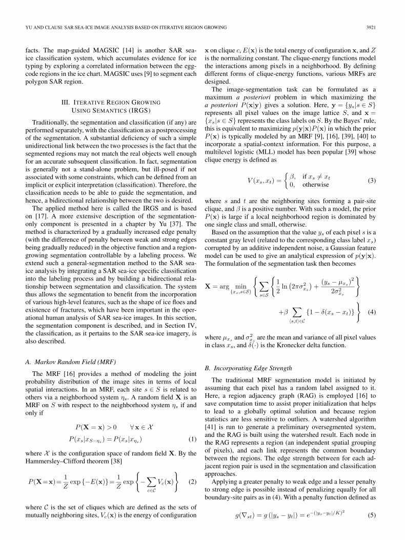
Fig. 2. Segmentation and classification of a SAR sea-ice image captured over the Gulf of St. Lawrence on February 20, 1998. The image size is 1209 × 865. Ithas three classes: Water, gray ice, and gray–white ice. (a) Original SAR image. (b) Result using V-MLL. Note that open water is incorrectly identified throughoutthe gray–white region. (c) IRGS result without the high-level knowledge. Note that the gray and gray–white ice labels are reversed. (d) and (e) IRGS after 8 and34 iterations. Note that the gray and gray–white ice labels are reversed. (f) IRGS after 77 iterations. Note that, at this point, the gray and gray–white ice labelsare now properly assigned to the regions. In (b)–(f), white indicates masked land regions not included in the computation. Bright lines in (e) and (f) outline theboundaries of detected floes. The gray-scale coding of the segmentation in (b) and (c) selects the same four levels used for ice types in (d)–(f) to satisfy visualcomparisons.


Compared to (7), the merging criterion of (21) considers theshape of the regions in addition to the regional homogeneityand boundary strength. For example, if both Ωi and Ωj arewell-defined floes with a moderate length of common boundary,the merging result Ωk is likely far from the ellipse shape and,hence, is grouped in the nonfloe cluster. The related energydifference

V(el)1 (xk) − V

(el)1 (xi) − V

(el)1 (xj) (23)

is relatively high. Thus, this merging operation may be prohib-ited due to a possible positive energy difference in (21).

The merging is only allowed between regions belonging tothe same class and does not change the class label. As such, Oxi

in (15) is fixed during the merging operations. Therefore, V (el)1

is only proportional to the region size, no matter which of thetwo situations in (15) the region belongs to. If all three regionsΩi, Ωj , and Ωk belong to the same one of the two situations in(15), the energy difference in (23) is just zero since the regionsize of the merging result Ωk is the sum of those of Ωi andΩj . Thus, the floe-shape information does not play a role inthe merging criterion when all the three regions are floes (ornonfloes).

By the same philosophy, the energy difference related toV

(co)2 is always zero. Moreover, if the merging does not change

the relative brightness between the neighboring regions of dif-ference classes, which is usually the case, the energy differencerelated to V

(td)2 is also zero. This is the reason why both V

(td)2

and V(co)2 do not show up in the merging criterion (21).

In the region-based labeling process, we first group theregions into several clusters based on their provisional ice-type labels from previous runs, as in Table III. It is sometimesnecessary to change the labels of all regions belonging to thesame cluster together rather than change them individually.For example, at the initial stages of the processing in Fig. 2,hundreds of small regions exist in the center of the image cor-responding to the relatively brighter gray ice. However, such acluster of regions is labeled as gray–white ice in the first severalruns since the tone-difference knowledge indicates that brighterregions correspond to thicker ice. As the iteration continues, thetwo-cluster (floe versus nonfloe) hypothesis becomes true at acertain scale. Floe information begins to play a role, makingit possible for this cluster of regions to change their labels togray ice. If the labeling is on individual regions, the process willbe extremely slow and may easily be trapped in an inaccurateconfiguration. Therefore, we first try to minimize the energy ona region cluster base. This is allowed to be an exhaustive searchsince the number of clusters is not more than five (in addition towater, the egg-code definition allows at most four different icetypes). Individual regions are then investigated, and their labelsare updated separately.

The overall algorithm is shown in Table IV.

E. Parameters and Adaptive Weighting

The parameters for clique-energy functions are selected bytrial and error. Here, the trial range of weights C(td), C(ld)

1 ,

C(el)1 , and C(co) is set around one ([0.1, 10]) so that the

importance of the corresponding clique-energy functions is ap-

TABLE IVALGORITHM OF THE SAR SEA-ICE IRGS ANALYSIS

TABLE VSUMMARY OF THE CLIQUE-ENERGY PARAMETERS

FOR HIGH-LEVEL CLASSIFICATION

proximately at the same level as that of the segmentation energyin the overall objective function in (18). The two thresholdsC

(ld)2 and C(el)

2 have physical meanings and are adjusted aroundintuitively reasonable values. In the trials for each parameter,only the corresponding energy function is used, and all othersamong (10), (11), (15), and (17) are taken out. Two SAR sea-ice images have been selected for the trials, and the obtainedbest parameters have been found applicable to all other 17images tested in our experiments. The parameter values aresummarized in Table V. The sensitivity of the overall solutionto these parameters is reasonably low since the parameters canbe adjusted around the selected values within a moderate rangewithout changing the essence of the final result. For example,the range [0.2, 2] for C(el)

1 produces similar results.In practice, we may want to have a variable weighting

instead of a constant weighting between the segmentation andclassification energy terms [47], or between different expertknowledge. For example, tone information is more reliable thanothers (e.g., shape) at the early stages of the process whenthe obtained regions are highly probable to be oversegmented.Therefore, we multiplied the two tone-related clique-energyfunctions V1(·) and V

(td)2 (·) with a weight, which decreases

with increasing iterations, as shown in the following equation:

Wk+1 = 0.9Wk + 0.1 (24)

where Wk is the weight for iteration k, and W0 is an initialvalue set as 80 in this paper. The weight is lower-limited to oneby the equation.


V. EXPERIMENTS AND DISCUSSIONS

The method is tested on 19 SAR sea-ice images, processedand provided by the CIS, of eight different scenes coveringvarious regions such as Baffin Bay, Gulf of St. Lawrence, andBeaufort Sea, and in various seasons as well. They are allacquired by RADARSAT in ScanSAR C-band mode and have aresolution of 100 m (images of 50-m resolution are 2 × 2 block-averaged by the CIS). Five examples are included in this paper.Due to the difficulty of obtaining the pixel-level ground truth,the experiment results are evaluated subjectively. An onlinemeeting with experts in the CIS was held on April 26, 2006for such an evaluation. In addition, a comparison is performed(with respect to the segmentation goal) between the proposedIRGS system and a recent SAR sea-ice segmentation approach[9] named (V-MLL) here, which uses a variable weightingbetween the feature model and the MLL context model.

The egg code is provided as an input to improve the effec-tiveness and reliability, as mentioned in Section I. However,the only egg-code information utilized by the system is theice types existing in the egg-code region. An information ofconcentration and floe size has been ignored because it is highlysubjective. Therefore, the system has only the knowledge of thenumber and names of ice classes. It is also possible to inferfrom the ice chart other information, such as a coarse estimateof the tone of a specific ice class, by exploring the correlationsbetween the various egg-code regions of the same ice chart [14].However, the success of such information extraction depends onthe correctness and information richness of the ice chart. Thispaper deals with the individual egg-code region only.

The first test sample is shown in Fig. 2(a). The correspondingtask is a three-class segmentation and classification amongwater, gray ice, and gray–white ice. The center of the bottomis land, which is excluded from all computations and is rep-resented by white regions in Fig. 2(b)–(f). The dark regionsurrounding the land is water. Regions having dark ice floeswith brighter ridges in between are gray–white ice, and therest are gray ice. The difficulty of this task lies in both thesegmentation and the classification parts. The segmentationis greatly influenced by heavy noise and the large intraclassvariations of the gray–white ice, whereas the classificationrelies on floe and leads information for correct identificationof ice types. The V-MLL gives a highly oversegmented resultin Fig. 2(b), and many dark gray–white ice floes are mistakenlyassigned the same label as the water. The IRGS system givesa satisfactory segmentation result in Fig. 2(f), having achieveda good balance between region consistency and detail preser-vation. In the result, those bright lines show the boundaries offloes detected during the process. Some leads are too narrowto be accurately captured by the initial watershed and, thus, arelost by subsequent merging processes. Although some floes andsegments of leads are missing, the detected floes and leads playan important role in correctly distinguishing between gray iceand gray–white ice.

To demonstrate this, intermediate results have been includedin Fig. 2(d) and (e). Early stages of the process produce resultsof similar level of quality as V-MLL, as shown in Fig. 2(d), ifthe bright leads in the figure are also considered to be water.Here, the large population of lead labels (even in the waterregion) is caused by the initial large amount of tiny regions

among which some happen to be elongated and dark. BecauseFig. 2(d) is too oversegmented (average region size is 149),there is not a distinct cluster of floe regions, and the floe-shapeenergy (15) is always zero and does not play a role. As aresult, the classifications of the segmented regions are mainlybased on tone, and the labeling of gray ice and gray–whiteice has been mistakenly reversed since the tone energy of (10)always classifies brighter regions with thicker ice types. Asmore iterations have been completed, tiny regions are merged,and the regions corresponding to floes begin to appear. Atiteration 34, some floes are detected, as shown in Fig. 2(e).However, the population of the detected gray–white ice floesis not yet large enough to reverse the labeling of the gray iceand gray–white ice at this stage. As the process continues, moreand larger gray–white ice-floe regions are obtained, and moreaccurate classifications of the segmented regions are possible.The final result in Fig. 2(f) has preserved most floes detectedduring all the iterations and distinguished correctly between thegray ice and gray–white ice.

The previous paragraph shows how the segmentation influ-ences the classification. On the other hand, the segmentationis also influenced by the classification in the IRGS process.Fig. 2(c) shows the IRGS result without including the high-level knowledge clique functions of (10), (11), (15), and (17).This segmentation result is better than that of the V-MLL in pro-ducing large homogeneous regions for gray ice and gray–whiteice but is inferior in preserving the lead regions. By comparingFig. 2(c) and (f), it is clear that an improvement in detailpreservations has been achieved by incorporating the high-levelknowledge that favors semantic meaningful configurations. Forexample, a lead and a gray-ice region not observed in Fig. 2(c)appears in the top left of Fig. 2(f) due to the influence ofthe domain knowledge that favors the elongated shape anddark tone of the lead region and the cooccurrence of gray iceand leads.

For better understanding of the role of various high-levelknowledge, different combinations of their clique functions,with others discarded, have been included in the segmentationand classification processes. Fig. 3 shows some examples. InFig. 3(a), only the elongated-shape energy (11) is included.As the system knows nothing about whether a lead should bebright or dark, many bright ridges are labeled as leads. For thesame reason, there is no information for making decisions forother classes, and hence, the other class labels are randomlydetermined. Compared to Fig. 2(c), more details have been pre-served for the bright ridges by chance due to the incorporationof the elongated-shape energy which is designed to describethe lead shape. Knowledge of the cooccurrence of classes isthen incorporated in Fig. 3(b) in addition to the elongated-shape energy. This knowledge favors the cooccurrence of leadsand the thinner of the two ice types—gray ice. Again, brightridges are mistakenly identified as leads, as in Fig. 3(a), andthe gray–white regions are mistakenly identified as gray sincethey are neighboring to the identified “leads.” Greater preser-vation of details has been achieved by the incorporation ofsuch knowledge, although the classification is still incorrect.To solve the problem, tone information has to be included,and the corresponding result is shown in Fig. 3(c). The ridgesare no longer mistaken as leads, but the labels of gray iceand gray–white ice are reversed. Correction of this reversal


Fig. 3. Different combinations of high-level knowledge cliques in the seg-mentation and classification in Fig. 2(a). (a) Only elongated shape (11) in-cluded. (b) Elongated shape (11) and cooccurrence of classes (17) included.(c) Elongated shape (11), cooccurrence of classes (17), and tone difference (10)included.

Fig. 4. Segmentation and classification of a SAR sea-ice image captured overthe Baffin Bay on February 7, 1998. The size is 1212 × 862. It has two classes:medium first-year ice and thick first-year ice. In (c), bright lines outline theboundaries of detected floes. The gray-scale coding of the segmentation in(b) selects the same two levels used for ice types in (c) for visual-comparisonneed. (a) Original. (b) V-MLL result. (c) IRGS result.


Fig. 5. Segmentation and classification of a SAR sea-ice image captured overthe Beaufort sea on October 13, 1997. The size is 1212 × 860. It has threeclasses: water, new ice, and gray ice. (a) Original. (b) IRGS result.

requires floe knowledge, as already mentioned in the previousparagraph.

Fig. 4(a) shows another example showing the importance ofthe floe information. The image consists of two ice types—medium first-year ice and thick first-year ice. The thicker of thetwo can be identified by dark well-defined floes and dominatesthe right part of the image. Again, the bright lines in Fig. 4(c)show that some of those floes have been detected and resultin the correct discrimination between the two ice types. It canclearly be found that many visually obvious floe regions are notquite elliptic; thus, our ellipse description of the floe shape isnot always suitable. For the segmentation quality, the V-MLL inFig. 4(b) has preserved more details than the IRGS in Fig. 4(c).However, it is difficult to conclude which is better due to theunavailability of the ground truth data.

Fig. 5(a) consists of three classes—water, new ice, and grayice. In the gray-ice region, in the bottom of the image, there aresome small ice floes with gaps in between. The obtained IRGSresult in Fig. 5(b) consists of large regions and does not preservethose gaps well. On the other hand, new ice does not have

Fig. 6. Segmentation and classification of a SAR sea-ice image captured overthe Beaufort sea on October 13, 1997. The size is 1212 × 856. It has twoclasses: gray ice and multiyear ice. (a) Original. (b) IRGS result.

clear boundaries but ambiguous transition regions to water. Thequality of the details in the new-ice regions is difficult to evalu-ate due to the ambiguity of those classes. In the bottom-rightcorner, the relatively brighter water region (probably causedby wind and incidence-angle effects) is separated from thesurrounding darker water and is classified as new ice. Correctidentification of this water region probably needs to rely onother features, for example, textures, as the textural appearanceof this water region looks quite similar to the large water bodyin the left of the image. Another possible scheme is to divide theopen water into two classes: one rough and one smooth. Theseconcepts are planned as part of future work.

Two other examples are shown in Figs. 7 and 8, respectively.Subjectively, satisfactory segmentations have been obtained,and correct ice identifications are achieved. An error hasoccurred in the bottom-right corner of Fig. 6, where the mul-tiyear ice is relatively dark due to snow cover and has beenmistakenly labeled as gray ice.

Since the IRGS is region-based and the number of regionskeeps decreasing by the merging process, the computation


Fig. 7. Segmentation and classification of a SAR sea-ice image captured overthe Baffin Bay on February 7, 1998. The size is 1212 × 862. It has two classes:thick first-year ice and second-year ice. The white regions belong to other egg-code regions and are not involved in computation. (a) Original. (b) IRGS result.

speed is much faster than the pixel-based methods such asV-MLL. For the tested images, the average execution time byIRGS is 94 s, whereas that of the V-MLL is 338 s for the samenumber of iterations on a Toshiba laptop of P3 800 MHz with128MB RAM. These are both within the range of acceptableclassification times in support of operational ice mapping.

VI. SUMMARY AND FUTURE WORK

We present in this paper a joint segmentation and classi-fication system for SAR sea-ice analysis. The segmentationalgorithm is based on a region-growing technique, and the clas-sification is a region-based MRF approach. The two processesare integrated under the Bayesian framework, with both aimingat reducing a defined energy. The interactions between the twoare bidirectional by letting the classification result to have somedegree of control on the region-growing process. Various low-level features and high-level knowledge can hence be efficiently

combined, and the system performs successfully with the testedSAR sea-ice images.

The proposed system performs the solution searching ina bottom-up manner on the hierarchical structure establishedduring the process. More accurate results could also be obtainedwith a subsequent top-down searching and adaptive updatingof the structure. Also, the ice-floe-shape descriptor may beimproved by a more general class of curves [48].

All experimental results are evaluated subjectively due tothe difficulty of obtaining the pixel-level ground truth. Thehuman expert interpretations agree with the experimental re-sults. Although such an evaluation is qualitative, our system isa practical solution to the identifications of difficult ice types,such as gray ice and gray–white ice, which, to our knowledge,has not been explored before. Future works are required forquantitative evaluations.

ACKNOWLEDGMENT

The authors would like to thank the referees for their thought-ful and insightful reviews that helped improve the overallquality of this paper. RADARSAT images are copyrighted bythe Canadian Space Agency (CSA).

REFERENCES

[1] World Meteorology Organization, Dec. 17, 2005. [Online]. Available:http://www.wmo.ch/index-en.html

[2] A. Baraldi and F. Parmiggiani, “An investigation of the textural char-acteristics associated with gray level cooccurrence matrix statisticalparameters,” IEEE Trans. Geosci. Remote Sens., vol. 33, no. 2, pp. 293–304, Mar. 1995.

[3] D. G. Barber and E. F. LeDrew, “SAR sea ice discrimination using texturestatistics: A multivariate approach,” Photogramm. Eng. Remote Sens.,vol. 57, no. 4, pp. 385–395, 1991.

[4] A. V. Bogdanov, M. Toussaint, and S. Sandven, “Recurrent modu-lar network architecture for sea ice classification in the marginal icezone using ERS SAR images,” in Proc. SPIE—Image Signal Process.Remote Sens. XI, L. Bruzzone, Ed., Oct. 2005, vol. 5982, pp. 283–287.

[5] A. V. Bogdanov, S. Sandven, O. M. Johannessen, V. Y. Alexandrov, andL. P. Bobylev, “Multisensor approach to automated classification of seaice image data,” IEEE Trans. Geosci. Remote Sens., vol. 43, no. 7,pp. 1648–1664, Jul. 2005.

[6] M. E. Shokr, “Evaluation of second-order texture parameters for seaice classification from radar images,” J. Geophys. Res., vol. 96, no. C6,pp. 10 625–10 640, 1991.

[7] L. K. Soh and C. Tsatsoulis, “Texture analysis of SAR sea ice imageryusing gray level cooccurrence matrices,” IEEE Trans. Geosci. RemoteSens., vol. 37, no. 2, pp. 780–795, Mar. 1999.

[8] D. A. Clausi and B. Yue, “Comparing cooccurrence probabilities andMarkov random fields for texture analysis of SAR sea ice imagery,” IEEETrans. Geosci. Remote Sens., vol. 42, no. 1, pp. 215–228, Jan. 2004.

[9] H. Deng and D. A. Clausi, “Unsupervised segmentation of syntheticaperture radar sea ice imagery using a novel Markov random field model,”IEEE Trans. Geosci. Remote Sens., vol. 43, no. 3, pp. 528–538, Mar. 2005.

[10] R. Samadani, “A finite mixture algorithm for finding proportions in SARimages,” IEEE Trans. Image Process., vol. 4, no. 8, pp. 1182–1186,Aug. 1995.

[11] L. K. Soh and C. Tsatsoulis, “Unsupervised segmentation of ERS andradarsat sea ice images using multiresolution peak detection and aggre-gated population equalization,” Int. J. Remote Sens., vol. 20, no. 15/16,pp. 3087–3109, 1999.

[12] J. A. Karvonen, “Baltic sea ice SAR segmentation and classification usingmodified pulse-coupled neural networks,” IEEE Trans. Geosci. RemoteSens., vol. 42, no. 7, pp. 1566–1574, Jul. 2004.

[13] J. Karvonen, M. Simila, and M. Makynen, “Open water detection fromBaltic sea ice Radarsat-1 SAR imagery,” IEEE Geosci. Remote Sens. Lett.,vol. 2, no. 3, pp. 275–279, Jul. 2005.

[14] P. Maillard, D. A. Clausi, and H. Deng, “Operational map-guided clas-sification of SAR sea ice imagery,” IEEE Trans. Geosci. Remote Sens.,vol. 43, no. 12, pp. 2940–2951, Dec. 2005.


[15] L. K. Soh, C. Tsatsoulis, D. Gineris, and C. Bertoia, “ARKTOS: Anintelligent system for SAR sea ice image classification,” IEEE Trans.Geosci. Remote Sens., vol. 42, no. 1, pp. 229–248, Jan. 2004.

[16] S. Z. Li, Markov Random Field Modeling in Image Analysis. New York:Springer-Verlag, 2001.

[17] Q. Yu and D. A. Clausi, “Combining local and global features for imagesegmentation using iterative classification and region merging,” in Proc.2nd Can. Conf. Comput. Robot Vis., Victoria, BC, Canada, May 9–11,2005, pp. 579–586.

[18] Canadian Ice Service, Dec. 20, 2005. [Online]. Available: http://ice-glaces.ec.gc.ca

[19] J. Karvonen, M. Simila, and I. Heiler, “Ice thickness estimation usingSAR data and ice thickness history,” in Proc. IEEE Int. Geosci. RemoteSens. Symp., 2003, vol. 1, pp. 74–76.

[20] F. D. Carsey, Ed., Microwave Remote Sensing of Sea Ice. Washington,DC: AGU, 1992

[21] W. Dierking and T. Busche, “Sea ice monitoring by L-band SAR: Anassessment based on literature and comparisons of JERS-1 and ERS-1imagery,” IEEE Trans. Geosci. Remote Sens., vol. 44, no. 4, pp. 957–970,Apr. 2006.

[22] J. S. Lee, “Speckle analysis and smoothing of SAR images,” Comput.Graph. Image Process., vol. 17, no. 1, pp. 24–32, 1981.

[23] V. S. Frost, J. A. Stiles, K. S. Shanmugan, and J. C. Holtzman, “A modelfor radar images and its application to adaptive digital filtering of mul-tiplicative noise,” IEEE Trans. Pattern Anal. Mach. Intell., vol. PAMI-4,no. 2, pp. 157–166, Mar. 1982.

[24] D. T. Kuan, A. A. Sawchuk, T. C. Strand, and P. Chavel, “Adaptiverestoration of images with speckle,” IEEE Trans. Acoust., Speech, SignalProcess., vol. ASSP-35, no. 3, pp. 373–383, Mar. 1987.

[25] G. Ramponi and C. Moloney, “Smoothing speckled images using anadaptive rational operator,” IEEE Signal Process. Lett., vol. 4, no. 3,pp. 68–71, Mar. 1997.

[26] Y. Yu and S. T. Acton, “Speckle reducing anisotropic diffusion,” IEEETrans. Image Process., vol. 11, no. 11, pp. 1260–1270, Nov. 2002.

[27] M. P. Mäkynen, A. T. Manninen, M. H. Similä, J. A. Karvonen, andM. T. Hallikainen, “Incidence angle dependence of the statistical proper-ties of C-band HH-polarization backscattering signatures of the Baltic seaice,” IEEE Trans. Geosci. Remote Sens., vol. 40, no. 12, pp. 2593–2605,Dec. 2002.

[28] R. A. Shuchman, C. C. Wackerman, A. L. Maffett, R. G. Onstott, andL. L. Sutherland, “The discrimination of sea ice types using SARbackscatter statistics,” in Proc. Geosci. Remote Sens. Symp., Vancouver,BC, Canada, 1989, pp. 381–385.

[29] D. A. Clausi, “An analysis of cooccurrence texture statistics as afunction of grey level quantization,” Can. J. Remote Sens., vol. 28, no. 1,pp. 45–62, 2002.

[30] W. Yang, C. He, Y. Cao, H. Sun, and X. Xu, “Improved classificationof SAR sea ice imagery based on segmentation,” in Proc. IGARSS,Jul. 2006, pp. 3727–3730.

[31] B. A. Draper, R. T. Collins, J. Brolio, A. R. Hanson, and E. M. Riseman,“The schema system,” Int. J. Comput. Vis., vol. 2, no. 3, pp. 209–250,Jan. 1989.

[32] S. S. Hwang, L. S. Davis, and T. Matsuyama, “Hypothesis integrationin image understanding systems,” Comput. Vis. Graph. Image Process.,vol. 36, no. 2/3, pp. 321–371, 1986.

[33] C. E. Liedtke, J. Bückner, O. Grau, S. Growe, and R. Tönjes, “AIDA: Asystem for the knowledge based interpretation of remote sensing data,”in Proc. 3rd Int. Airborne Remote Sens. Conf. Exhib., Copenhagen,Denmark, Jul. 1997, vol. 2, pp. 313–320.

[34] H. Niemann, G. F. Sagerer, S. Schroder, and F. Kummert, “Ernest: Asemantic network system for pattern understanding,” IEEE Trans. PatternAnal. Mach. Intell., vol. 12, no. 9, pp. 883–905, Sep. 1990.

[35] J. W. Modestino and J. Zhang, “A Markov random field model based ap-proach to image interpretation,” IEEE Trans. Pattern Anal. Mach. Intell.,vol. 14, no. 6, pp. 606–615, Jun. 1992.

[36] J. Pearl, Probabilistic Reasoning in Intelligent Systems: Networks of Plau-sible Inference. San Mateo, CA: Morgan Kaufmann, 1988.

[37] Q. Yu, “Automated SAR sea ice interpretation,” Ph.D. dissertation, Dept.Syst. Design Eng., Univ. Waterloo, Waterloo, ON, Canada, 2006.

[38] J. Besag, “Spatial interaction and the statistical analysis of lattice sys-tems,” J. R. Stat. Soc., Ser. B, vol. 36, no. 2, pp. 192–236, 1974.

[39] H. Derin and H. Elliott, “Modeling and segmentation of noisy and texturedimages using Gibbs random fields,” IEEE Trans. Pattern Anal. Mach.Intell., vol. PAMI-9, no. 1, pp. 39–55, Jan. 1987.

[40] C. S. Won and H. Derin, “Unsupervised segmentation of noisy and tex-tured images using Markov random fields,” CVGIP, Graph. Models ImageProcess., vol. 54, no. 4, pp. 308–328, 1992.

[41] L. Vincent and P. Soille, “Watershed in digital spaces: An efficient algo-rithm based on immersion simulations,” IEEE Trans. Pattern Anal. Mach.Intell., vol. 13, no. 6, pp. 583–598, Jun. 1991.

[42] J. A. Feldman and Y. Yakimovsky, “Decision theory and artificial intel-ligence I: Semantics-based region analyzer,” Artif. Intell., vol. 5, no. 4,pp. 349–371, 1974.

[43] M. Sonka, V. Hlavac, and R. Boyle, Image Processing, Analysis, andMachine Vision. Boston, MA: Thomson Course Technology, 1998.

[44] A. Barbu and S. C. Zhu, “Generalizing Swendsen-Wang to samplingarbitrary posterior probabilities,” IEEE Trans. Pattern Anal. Mach. Intell.,vol. 27, no. 8, pp. 1239–1253, Aug. 2005.

[45] M. K. Hu, “Visual pattern recognition by moment invariants,” IRE Trans.Inf. Theory, vol. 8, no. 2, pp. 179–187, 1961.

[46] R. O. Duda, P. E. Hart, and D. G. Stork, Pattern Classification. Hoboken,NJ: Wiley, 2001.

[47] I. Y. Kim and H. S. Yang, “An integration scheme for image segmentationand labelling based on Markov random field model,” IEEE Trans. PatternAnal. Mach. Intell., vol. 18, no. 1, pp. 69–73, Jan. 1996.

[48] J. Banfield, “Automated tracking of ice floes: A stochastic approach,”IEEE Trans. Geosci. Remote Sens., vol. 29, no. 6, pp. 905–911,Nov. 1991.

Qiyao Yu received the B.A.Sc. degree from Ts-inghua University, Beijing, China, in 1997, theM.A.Sc. degree from the Memorial University ofNewfoundland, St. John’s, NF, Canada, in 2002, andthe Ph.D. degree in systems design engineering fromthe University of Waterloo, Waterloo, ON, Canada,in 2006.

He is currently with Eutrovision Inc., Shanghai,China. His research interest is in image and videoprocessing, pattern recognition, and remote sensing.

David A. Clausi (S’93–M’96–SM’03) received theB.A.Sc., M.A.Sc., and Ph.D. degrees in systemsdesign engineering from the University of Waterloo,Waterloo, ON, Canada, in 1990, 1992, and 1996,respectively.

After completing his doctorate, he worked inthe medical imaging field with Mitra Imaging Inc.,Waterloo. He started his academic career in 1997 asan Assistant Professor in geomatics engineering withthe University of Calgary, Calgary, AB, Canada. In1999, he returned to the University of Waterloo and

was awarded tenure and promotion to Associate Professor in 2003, where heis currently with the Department of Systems Design Engineering. He is anactive Interdisciplinary and Multidisciplinary Researcher. He has an extensivepublication record, publishing refereed journal and conference papers in diversefields of remote sensing, computer vision, algorithm design, and biomechanics.His primary research interest is automated interpretation of synthetic apertureradar sea-ice imagery in support of the operational activities of the CanadianIce Service. The research results have successfully led to commercial imple-mentations.

Dr. Clausi has received numerous scholarships, conference paper awards, andtwo Teaching Excellence Awards.

sar sea-ice image analysis based on iterative region ...dclausi/papers/published 2007/yu and...

Documents