sas scalable performance data (spd) server 4.5: user's guide

SAS® Scalable Performance Data Server® 4.5User’s Guide

TW10910_colortitlepg.indd 1 5/26/09 3:23:52 PM

The correct bibliographic citation for this manual is as follows: SAS Institute Inc. 2009. SAS® Scalable Performance Data Server® 4.5: User’s Guide. Cary, NC: SAS Institute Inc.

SAS® Scalable Performance Data Server® 4.5: User’s Guide

Copyright © 2009, SAS Institute Inc., Cary, NC, USA

All rights reserved. Produced in the United States of America.

For a hard-copy book: No part of this publication may be reproduced, stored in a retrieval system, or transmitted, in any form or by any means, electronic, mechanical, photocopying, or otherwise, without the prior written permission of the publisher, SAS Institute Inc.

For a Web download or e-book: Your use of this publication shall be governed by the terms established by the vendor at the time you acquire this publication.

U.S. Government Restricted Rights Notice: Use, duplication, or disclosure of this software and related documentation by the U.S. government is subject to the Agreement with SAS Institute and the restrictions set forth in FAR 52.227-19, Commercial Computer Software-Restricted Rights (June 1987).

SAS Institute Inc., SAS Campus Drive, Cary, North Carolina 27513.

1st electronic book, June 2009

SAS® Publishing provides a complete selection of books and electronic products to help customers use SAS software to its fullest potential. For more information about our e-books, e-learning products, CDs, and hard-copy books, visit the SAS Publishing Web site at support.sas.com/publishing or call 1-800-727-3228.

SAS® and all other SAS Institute Inc. product or service names are registered trademarks or trademarks of SAS Institute Inc. in the USA and other countries. ® indicates USA registration.

Other brand and product names are registered trademarks or trademarks of their respective companies.

Contents

PART 1 Product Notes 1

Chapter 1 • SAS Scalable Performance Data (SPD) Server Product Notes . . . . . . . . . . . . . . . . . 3Overview . . . . . . . . . . . . . . . . . . . . . . . . . . . . . . . . . . . . . . . . . . . . . . . . . . . . . . . . . . . . . . 3What's New in SPD Server 4.5? . . . . . . . . . . . . . . . . . . . . . . . . . . . . . . . . . . . . . . . . . . . . 3SPD Server 4.5 Platform Support Changes . . . . . . . . . . . . . . . . . . . . . . . . . . . . . . . . . . . 4

PART 2 SPD Server Usage 5

Chapter 2 • SAS Scalable Performance Data (SPD) Server Overview . . . . . . . . . . . . . . . . . . . . . . 7Introduction to SAS Scalable Performance Data (SPD) Server . . . . . . . . . . . . . . . . . . . . 7The SPD Server Client/Server Model . . . . . . . . . . . . . . . . . . . . . . . . . . . . . . . . . . . . . . . . 8Accessing SPD Server Using SAS . . . . . . . . . . . . . . . . . . . . . . . . . . . . . . . . . . . . . . . . . 11Securing SAS Data . . . . . . . . . . . . . . . . . . . . . . . . . . . . . . . . . . . . . . . . . . . . . . . . . . . . . 13Organizing SAS Data . . . . . . . . . . . . . . . . . . . . . . . . . . . . . . . . . . . . . . . . . . . . . . . . . . . 14SPD Server Performance Enhancements . . . . . . . . . . . . . . . . . . . . . . . . . . . . . . . . . . . . 16SPD Server Extensions to Base SAS . . . . . . . . . . . . . . . . . . . . . . . . . . . . . . . . . . . . . . . 17Using SPD Server with Data Warehousing . . . . . . . . . . . . . . . . . . . . . . . . . . . . . . . . . . 17

Chapter 3 • Connecting to SAS Scalable Performance Data (SPD) Server . . . . . . . . . . . . . . . . . 19Introduction . . . . . . . . . . . . . . . . . . . . . . . . . . . . . . . . . . . . . . . . . . . . . . . . . . . . . . . . . . . 19SAS and SPD Server Tables . . . . . . . . . . . . . . . . . . . . . . . . . . . . . . . . . . . . . . . . . . . . . . 20SPD ServerResource Security . . . . . . . . . . . . . . . . . . . . . . . . . . . . . . . . . . . . . . . . . . . . 21Accessing SPD Server from a SAS Client . . . . . . . . . . . . . . . . . . . . . . . . . . . . . . . . . . . 22SPD Server Table Options . . . . . . . . . . . . . . . . . . . . . . . . . . . . . . . . . . . . . . . . . . . . . . . 26SPD Server Macro Variables . . . . . . . . . . . . . . . . . . . . . . . . . . . . . . . . . . . . . . . . . . . . . 27

Chapter 4 • Accessing and Creating SAS Scalable Performance Data (SPD)Server Tables . . . . . . . . . . . . . . . . . . . . . . . . . . . . . . . . . . . . . . . . . . . . . . . . . . . . . . . . . . . . . . . 31

Introduction . . . . . . . . . . . . . . . . . . . . . . . . . . . . . . . . . . . . . . . . . . . . . . . . . . . . . . . . . . . 31Using a LIBNAME Statement to Access SPD Server . . . . . . . . . . . . . . . . . . . . . . . . . . 32Managing Large SPD Server Files . . . . . . . . . . . . . . . . . . . . . . . . . . . . . . . . . . . . . . . . . 33Migrating Tables between SAS and SPD Server . . . . . . . . . . . . . . . . . . . . . . . . . . . . . . 39The SQL Pass-Through Facility . . . . . . . . . . . . . . . . . . . . . . . . . . . . . . . . . . . . . . . . . . . 40Creating a New Table . . . . . . . . . . . . . . . . . . . . . . . . . . . . . . . . . . . . . . . . . . . . . . . . . . . 44

Chapter 5 • Indexing, Sorting, and Manipulating SAS Scalable PerformanceData (SPD) Server Tables . . . . . . . . . . . . . . . . . . . . . . . . . . . . . . . . . . . . . . . . . . . . . . . . . . . . . . 47

Introduction . . . . . . . . . . . . . . . . . . . . . . . . . . . . . . . . . . . . . . . . . . . . . . . . . . . . . . . . . . . 47Indexing a Table . . . . . . . . . . . . . . . . . . . . . . . . . . . . . . . . . . . . . . . . . . . . . . . . . . . . . . 47Creating SPD Server Indexes Examples . . . . . . . . . . . . . . . . . . . . . . . . . . . . . . . . . . . . . 48

Chapter 6 • Using SAS Scalable Performance Data (SPD) Server with Other Clients . . . . . . . . 53Overview . . . . . . . . . . . . . . . . . . . . . . . . . . . . . . . . . . . . . . . . . . . . . . . . . . . . . . . . . . . . . 53Using Open Database Connectivity (ODBC) to Access SPD Server Tables . . . . . . . . . 54Using JDBC (Java) to Access SPD Server Tables . . . . . . . . . . . . . . . . . . . . . . . . . . . . 59Using htmSQL to Access SPD Server Tables . . . . . . . . . . . . . . . . . . . . . . . . . . . . . . . . 62

Using SQL C API to Access SPD Server Tables . . . . . . . . . . . . . . . . . . . . . . . . . . . . . . 64

Chapter 7 • SAS Scalable Performance Data (SPD) Server Dynamic Cluster Tables . . . . . . . . 65Introduction to Dynamic Cluster Tables . . . . . . . . . . . . . . . . . . . . . . . . . . . . . . . . . . . . . 65Dynamic Cluster Table Structure . . . . . . . . . . . . . . . . . . . . . . . . . . . . . . . . . . . . . . . . . 66Benefits of Dynamic Cluster Tables . . . . . . . . . . . . . . . . . . . . . . . . . . . . . . . . . . . . . . . 67Creating and Controlling Dynamic Cluster Tables . . . . . . . . . . . . . . . . . . . . . . . . . . . . 68Dynamic Cluster BY Clause Optimization . . . . . . . . . . . . . . . . . . . . . . . . . . . . . . . . . . 76Member Table Requirements for Creating Dynamic Cluster Tables . . . . . . . . . . . . . . 79Querying and Reading Member Tables in a Dynamic Cluster . . . . . . . . . . . . . . . . . . . . 82Unsupported Features in Dynamic Cluster Tables . . . . . . . . . . . . . . . . . . . . . . . . . . . . 83Dynamic Cluster Table Examples . . . . . . . . . . . . . . . . . . . . . . . . . . . . . . . . . . . . . . . . . 84

PART 3 SPD Server SQL Features 91

Chapter 8 • SPD Server SQL Features . . . . . . . . . . . . . . . . . . . . . . . . . . . . . . . . . . . . . . . . . . . . . . 93SPD Server SQL Planner . . . . . . . . . . . . . . . . . . . . . . . . . . . . . . . . . . . . . . . . . . . . . . . . 94Connecting to the SPD Server SQL Engine . . . . . . . . . . . . . . . . . . . . . . . . . . . . . . . . . . 95Specifying SPD Server SQL Planner Options . . . . . . . . . . . . . . . . . . . . . . . . . . . . . . . . 97Important SPD Server SQL Planner Options . . . . . . . . . . . . . . . . . . . . . . . . . . . . . . . . . 98Parallel Join Facility . . . . . . . . . . . . . . . . . . . . . . . . . . . . . . . . . . . . . . . . . . . . . . . . . . 105Parallel Group-By Facility . . . . . . . . . . . . . . . . . . . . . . . . . . . . . . . . . . . . . . . . . . . . . . 108Parallel Group-By SQL Options . . . . . . . . . . . . . . . . . . . . . . . . . . . . . . . . . . . . . . . . . 112SPD Server STARJOIN Facility . . . . . . . . . . . . . . . . . . . . . . . . . . . . . . . . . . . . . . . . . 113STARJOIN Options . . . . . . . . . . . . . . . . . . . . . . . . . . . . . . . . . . . . . . . . . . . . . . . . . . . 114STARJOIN Facility Reference . . . . . . . . . . . . . . . . . . . . . . . . . . . . . . . . . . . . . . . . . . . 115SPD Server Index Scan . . . . . . . . . . . . . . . . . . . . . . . . . . . . . . . . . . . . . . . . . . . . . . . . 127Optimizing Correlated Queries . . . . . . . . . . . . . . . . . . . . . . . . . . . . . . . . . . . . . . . . . . 130Correlated Query Options . . . . . . . . . . . . . . . . . . . . . . . . . . . . . . . . . . . . . . . . . . . . . . 130Materialized Views . . . . . . . . . . . . . . . . . . . . . . . . . . . . . . . . . . . . . . . . . . . . . . . . . . . 132SPD Server SQL Extensions . . . . . . . . . . . . . . . . . . . . . . . . . . . . . . . . . . . . . . . . . . . . 134Differences between SAS SQL and SPD Server SQL . . . . . . . . . . . . . . . . . . . . . . . . 141

PART 4 SPD Server SQL Reference 143

Chapter 9 • SPD Server SQL Syntax Reference Guide . . . . . . . . . . . . . . . . . . . . . . . . . . . . . . . . 145Overview . . . . . . . . . . . . . . . . . . . . . . . . . . . . . . . . . . . . . . . . . . . . . . . . . . . . . . . . . . . . 146Document Conventions . . . . . . . . . . . . . . . . . . . . . . . . . . . . . . . . . . . . . . . . . . . . . . . . 146SQL Syntax Definitions . . . . . . . . . . . . . . . . . . . . . . . . . . . . . . . . . . . . . . . . . . . . . . . . 147SQL Statements . . . . . . . . . . . . . . . . . . . . . . . . . . . . . . . . . . . . . . . . . . . . . . . . . . . . . . 148NEW SQL Statements . . . . . . . . . . . . . . . . . . . . . . . . . . . . . . . . . . . . . . . . . . . . . . . . . 151SQL Building Blocks . . . . . . . . . . . . . . . . . . . . . . . . . . . . . . . . . . . . . . . . . . . . . . . . . . 152

Chapter 10 • SAS Scalable Performance Data (SPD) Server SQL AccessLibrary API Reference . . . . . . . . . . . . . . . . . . . . . . . . . . . . . . . . . . . . . . . . . . . . . . . . . . . . . . . 159

Introduction . . . . . . . . . . . . . . . . . . . . . . . . . . . . . . . . . . . . . . . . . . . . . . . . . . . . . . . . . . 159Overview of SPQL Usage . . . . . . . . . . . . . . . . . . . . . . . . . . . . . . . . . . . . . . . . . . . . . . 160SPQL API Description . . . . . . . . . . . . . . . . . . . . . . . . . . . . . . . . . . . . . . . . . . . . . . . . . 160SPQL API Functions . . . . . . . . . . . . . . . . . . . . . . . . . . . . . . . . . . . . . . . . . . . . . . . . . . 160SPQL Function Return Codes . . . . . . . . . . . . . . . . . . . . . . . . . . . . . . . . . . . . . . . . . . . 164

iv Contents

PART 5 SPD Server Reference 165

Chapter 11 • Optimizing SPD Server Performance . . . . . . . . . . . . . . . . . . . . . . . . . . . . . . . . . . . 167SPD Server Performance and Usage Tips . . . . . . . . . . . . . . . . . . . . . . . . . . . . . . . . . . 168Symmetric Multiple Processor (SMP) Utilization . . . . . . . . . . . . . . . . . . . . . . . . . . . . 168File System Performance Concepts . . . . . . . . . . . . . . . . . . . . . . . . . . . . . . . . . . . . . . . 169LIBNAME Domains . . . . . . . . . . . . . . . . . . . . . . . . . . . . . . . . . . . . . . . . . . . . . . . . . . . 171Loading Data into an SPD Server Host . . . . . . . . . . . . . . . . . . . . . . . . . . . . . . . . . . . . 172Table Loading Techniques . . . . . . . . . . . . . . . . . . . . . . . . . . . . . . . . . . . . . . . . . . . . . . 173Loading Indexes in Parallel . . . . . . . . . . . . . . . . . . . . . . . . . . . . . . . . . . . . . . . . . . . . . 174Truncating Tables . . . . . . . . . . . . . . . . . . . . . . . . . . . . . . . . . . . . . . . . . . . . . . . . . . . . . 176Optimizing WHERE clauses . . . . . . . . . . . . . . . . . . . . . . . . . . . . . . . . . . . . . . . . . . . . 177SPD Server Indexing . . . . . . . . . . . . . . . . . . . . . . . . . . . . . . . . . . . . . . . . . . . . . . . . . . 178WHERE Clause Planner . . . . . . . . . . . . . . . . . . . . . . . . . . . . . . . . . . . . . . . . . . . . . . . . 181How to Affect the WHERE Planner . . . . . . . . . . . . . . . . . . . . . . . . . . . . . . . . . . . . . . 187Identical Parallel WHERE Clause Subsetting Results . . . . . . . . . . . . . . . . . . . . . . . . . 189WHERE Clause Examples . . . . . . . . . . . . . . . . . . . . . . . . . . . . . . . . . . . . . . . . . . . . . . 191Server-Side Sorting . . . . . . . . . . . . . . . . . . . . . . . . . . . . . . . . . . . . . . . . . . . . . . . . . . . . 196

Chapter 12 • SPD Server Macro Variables . . . . . . . . . . . . . . . . . . . . . . . . . . . . . . . . . . . . . . . . . . 199Introduction . . . . . . . . . . . . . . . . . . . . . . . . . . . . . . . . . . . . . . . . . . . . . . . . . . . . . . . . . . 200Variable for Compatibility with the Base SAS Engine . . . . . . . . . . . . . . . . . . . . . . . . 200Variables for Miscellaneous Functions . . . . . . . . . . . . . . . . . . . . . . . . . . . . . . . . . . . . 201Variables for Sorts . . . . . . . . . . . . . . . . . . . . . . . . . . . . . . . . . . . . . . . . . . . . . . . . . . . . 206Variables for WHERE Clause Evaluations . . . . . . . . . . . . . . . . . . . . . . . . . . . . . . . . . 208Variables That Affect Disk Space . . . . . . . . . . . . . . . . . . . . . . . . . . . . . . . . . . . . . . . . 214Variables To Enhance Performance . . . . . . . . . . . . . . . . . . . . . . . . . . . . . . . . . . . . . . . 217Variables for a Client and a Server Running on the Same UNIX Machine . . . . . . . . . 219

Chapter 13 • SPD Server LIBNAME Options . . . . . . . . . . . . . . . . . . . . . . . . . . . . . . . . . . . . . . . . 221Introduction . . . . . . . . . . . . . . . . . . . . . . . . . . . . . . . . . . . . . . . . . . . . . . . . . . . . . . . . . . 222Options to Locate an SPD Server Host . . . . . . . . . . . . . . . . . . . . . . . . . . . . . . . . . . . . . 222Options to Identify the SPD Server Client . . . . . . . . . . . . . . . . . . . . . . . . . . . . . . . . . . 224Options to Specify Implicit SQL Pass-Through . . . . . . . . . . . . . . . . . . . . . . . . . . . . . . 227Options to Specify File Paths for Table Storage . . . . . . . . . . . . . . . . . . . . . . . . . . . . . 229Options for Access Control Lists (ACLs) . . . . . . . . . . . . . . . . . . . . . . . . . . . . . . . . . . 231Options for a Client and Server Running on the Same UNIX Machine . . . . . . . . . . . . 232Options for Other Functions . . . . . . . . . . . . . . . . . . . . . . . . . . . . . . . . . . . . . . . . . . . . . 233

Chapter 14 • SPD Server Table Options . . . . . . . . . . . . . . . . . . . . . . . . . . . . . . . . . . . . . . . . . . . . 245Introduction . . . . . . . . . . . . . . . . . . . . . . . . . . . . . . . . . . . . . . . . . . . . . . . . . . . . . . . . . . 245Option for Compatibility with Base SAS Software . . . . . . . . . . . . . . . . . . . . . . . . . . . 246Options That Affect Disk Space . . . . . . . . . . . . . . . . . . . . . . . . . . . . . . . . . . . . . . . . . . 247Options to Enhance Performance . . . . . . . . . . . . . . . . . . . . . . . . . . . . . . . . . . . . . . . . . 250Option to Test Performance . . . . . . . . . . . . . . . . . . . . . . . . . . . . . . . . . . . . . . . . . . . . . 252Options for WHERE Clause Evaluations . . . . . . . . . . . . . . . . . . . . . . . . . . . . . . . . . . . 254Options for Other Functions . . . . . . . . . . . . . . . . . . . . . . . . . . . . . . . . . . . . . . . . . . . . 258Options for Security . . . . . . . . . . . . . . . . . . . . . . . . . . . . . . . . . . . . . . . . . . . . . . . . . . . 267

Chapter 15 • SPD Server Formats and Informats . . . . . . . . . . . . . . . . . . . . . . . . . . . . . . . . . . . . 269Introduction . . . . . . . . . . . . . . . . . . . . . . . . . . . . . . . . . . . . . . . . . . . . . . . . . . . . . . . . . . 269Formats . . . . . . . . . . . . . . . . . . . . . . . . . . . . . . . . . . . . . . . . . . . . . . . . . . . . . . . . . . . . . 269User-Defined Formats Example . . . . . . . . . . . . . . . . . . . . . . . . . . . . . . . . . . . . . . . . . . 271Informats . . . . . . . . . . . . . . . . . . . . . . . . . . . . . . . . . . . . . . . . . . . . . . . . . . . . . . . . . . . . 275

Chapter 16 • SPD Server NLS Support . . . . . . . . . . . . . . . . . . . . . . . . . . . . . . . . . . . . . . . . . . . . . 277

Contents v

Overview of NLS . . . . . . . . . . . . . . . . . . . . . . . . . . . . . . . . . . . . . . . . . . . . . . . . . . . . . 277Character Encoding Overview . . . . . . . . . . . . . . . . . . . . . . . . . . . . . . . . . . . . . . . . . . . 278Moving Data across Environments with Different Encodings . . . . . . . . . . . . . . . . . . . 281Base SAS Encoding Behavior . . . . . . . . . . . . . . . . . . . . . . . . . . . . . . . . . . . . . . . . . . . 282Setting the Encoding for Base SAS Sessions . . . . . . . . . . . . . . . . . . . . . . . . . . . . . . . . 283Changing the Encoding for Base SAS Sessions . . . . . . . . . . . . . . . . . . . . . . . . . . . . . . 284NLS Support in SPD Server . . . . . . . . . . . . . . . . . . . . . . . . . . . . . . . . . . . . . . . . . . . . . 285

PART 6 Appendix 289

Chapter 17 • SPD Server Frequently Asked Questions . . . . . . . . . . . . . . . . . . . . . . . . . . . . . . . 291SPD Server Frequently Asked Questions . . . . . . . . . . . . . . . . . . . . . . . . . . . . . . . . . . . 292

vi Contents

Part 1

Product Notes

Chapter 1SAS Scalable Performance Data (SPD) Server Product Notes . . . . . . 3

1

Chapter 1SAS Scalable Performance Data(SPD) Server Product Notes

Overview . . . . . . . . . . . . . . . . . . . . . . . . . . . . . . . . . . . . . . . . . . . . . . . . . . . . . . . . . . . . . 3

What's New in SPD Server 4.5? . . . . . . . . . . . . . . . . . . . . . . . . . . . . . . . . . . . . . . . . . . 3Overview of SPD Server 4.5 . . . . . . . . . . . . . . . . . . . . . . . . . . . . . . . . . . . . . . . . . . . 3

SPD Server 4.5 Platform Support Changes . . . . . . . . . . . . . . . . . . . . . . . . . . . . . . . . . 4

OverviewThis document summarizes enhancements and changes in SPD Server 4.5.

• The SPD Server 4.5 installation includes client modules that are compatible with SAS9.2.

• SPD Server 4.5 is not compatible with SAS versions earlier than SAS 9.2. Refer to theappropriate SPD Server UNIX or Windows installation guide for more informationabout SAS software requirements for use with SPD Server 4.5.

What's New in SPD Server 4.5?

Overview of SPD Server 4.5The operating system requirements for SPD Server 4.5 have changed from the operatingsystem requirements for SPD Server 4.4. For more detailed information about operatingsystem requirements for SPD Server 4.5, see the Chapter 2, "SPD Server Pre-Installationand System Requirements Guide," in the SAS Scalable Performance Data (SPD) Server4.5: Administrator's Guide.

• SPD Audit logging has been enhanced to include the user LIBNAME in the proxy andSQL audit logs. For additional information, see the section on SPD Server Auditing inChapter 14, ACL Security Overview, of the SAS Scalable Performance Data (SPD)Server 4.5: Administrator's Guide.

• You can now specify recycle times for the SPD Server Name Server log and the SPDServer snet log. For additional information about configuring SPD Server log cycletimes for Windows installations, see the section, "Configuring SPD Server Softwareon your Windows Host" in Chapter 4, "SPD Server Windows Installation Guide," ofthe SAS Scalable Performance Data (SPD) Server 4.5: Administrator's Guide. For

3

additional information about configuring SPD Server log cycle times for UNIXinstallations, see "Configuring SPD Server Host Software for Your Site" in Chapter 3,"SPD Server UNIX Installation Guide," of the SAS Scalable Performance Data (SPD)Server 4.5: Administrator's Guide.

• SPD Server now supports user formats with the put() function that are greater than 8characters in length. An SPD Server host can read user format catalog files that werecreated by SAS running on Windows, or on the same machine as the SPD Server host.The spdsls list utility has been enhanced to add a -verbose option. The -verboseoption provides information such as the number of observations, observation length,index segment size, partition size, and whether the table is compressed, encrypted, oris a member of a cluster. For more information about SPD Server list utilities, see "SPDServer Table List Utility Spdsls," in Chapter 18 of the SAS Scalable Performance Data(SPD) Server 4.5: Administrator's Guide.

• SAS implicit pass-through SQL now permits SQL queries to SPD Server that includesupported SPD Server functions. contains a section, Chapter 8 of the SAS ScalablePerformance Data (SPD) Server 4.5: User's Guide, "SPD Server SQL Features"contains a section “Differences between SAS SQL and SPD Server SQL ” on page141that lists the functions that SPD Server supports via implicit pass-through SQL.

• The installation and delivery of the SPD Server 4.5 client components for SAS is nowpart of your SAS installation. For more detailed information about installing SPDServer 4.5 on a Windows platform, see Chapter 4, "SPD Server Windows InstallationGuide," of the SAS Scalable Performance Data (SPD) Server 4.5: Administrator'sGuide. For more detailed information about installing SPD Server 4.5 on a UNIXplatform, see Chapter 3, "SPD Server UNIX Installation Guide," of the SAS ScalablePerformance Data (SPD) Server 4.5: Administrator's Guide.

• The installation and delivery of SAS Management Console components for SPD Server4.5 is now part of your SAS Management Console installation. For more detailedinformation about installing SAS Management Console components for SPD Server4.5 on a Windows platform, see "Before You Install: Precautions and RequiredPermissions" in Chapter 4, "SPD Server Windows Installation Guide" of the SASScalable Performance Data (SPD) Server 4.5: Administrator's Guide. For moredetailed information about installing SAS Management Console components for SPDServer 4.5 on a UNIX platform, see, " Before You Install: Precautions and RequiredPermissions," in Chapter 3, "SPD Server UNIX Installation Guide" of the SAS ScalablePerformance Data (SPD) Server 4.5: Administrator's Guide.

SPD Server 4.5 Platform Support ChangesSPD Server 4.5 now supports Linux x64 platform.

4 Chapter 1 • SAS Scalable Performance Data (SPD) Server Product Notes

Part 2

SPD Server Usage

Chapter 2SAS Scalable Performance Data (SPD) Server Overview . . . . . . . . . . . 7

Chapter 3Connecting to SAS Scalable Performance Data (SPD) Server . . . . . 19

Chapter 4Accessing and Creating SAS Scalable Performance Data (SPD) ServerTables . . . . . . . . . . . . . . . . . . . . . . . . . . . . . . . . . . . . . . . . . . . . . . . . . . . . . . . . . . . 31

Chapter 5Indexing, Sorting, and Manipulating SAS Scalable Performance Data(SPD) Server Tables . . . . . . . . . . . . . . . . . . . . . . . . . . . . . . . . . . . . . . . . . . . . . 47

Chapter 6Using SAS Scalable Performance Data (SPD) Server with OtherClients . . . . . . . . . . . . . . . . . . . . . . . . . . . . . . . . . . . . . . . . . . . . . . . . . . . . . . . . . . 53

Chapter 7SAS Scalable Performance Data (SPD) Server Dynamic Cluster Tables. . . . . . . . . . . . . . . . . . . . . . . . . . . . . . . . . . . . . . . . . . . . . . . . . . . . . . . . . . . . . . . . . . 65

5

Chapter 2SAS Scalable Performance Data(SPD) Server Overview

Introduction to SAS Scalable Performance Data (SPD) Server . . . . . . . . . . . . . . . . . 7

The SPD Server Client/Server Model . . . . . . . . . . . . . . . . . . . . . . . . . . . . . . . . . . . . . . 8Overview of the Client/Server Model . . . . . . . . . . . . . . . . . . . . . . . . . . . . . . . . . . . . . 8Symmetric Multi-Processor Hosts . . . . . . . . . . . . . . . . . . . . . . . . . . . . . . . . . . . . . . . 9SPD Server Host Services for Clients . . . . . . . . . . . . . . . . . . . . . . . . . . . . . . . . . . . . 9

Accessing SPD Server Using SAS . . . . . . . . . . . . . . . . . . . . . . . . . . . . . . . . . . . . . . . . 11SQL Pass-Through Facility . . . . . . . . . . . . . . . . . . . . . . . . . . . . . . . . . . . . . . . . . . . 11LIBNAME Access . . . . . . . . . . . . . . . . . . . . . . . . . . . . . . . . . . . . . . . . . . . . . . . . . . 12SPD Server Host Name Server . . . . . . . . . . . . . . . . . . . . . . . . . . . . . . . . . . . . . . . . . 12Specifying the Port Address for the Name Server . . . . . . . . . . . . . . . . . . . . . . . . . . 13

Securing SAS Data . . . . . . . . . . . . . . . . . . . . . . . . . . . . . . . . . . . . . . . . . . . . . . . . . . . . 13LIBNAME Domain Registration . . . . . . . . . . . . . . . . . . . . . . . . . . . . . . . . . . . . . . . 13ACL File Security . . . . . . . . . . . . . . . . . . . . . . . . . . . . . . . . . . . . . . . . . . . . . . . . . . . 13

Organizing SAS Data . . . . . . . . . . . . . . . . . . . . . . . . . . . . . . . . . . . . . . . . . . . . . . . . . . 14SPD Server Tables . . . . . . . . . . . . . . . . . . . . . . . . . . . . . . . . . . . . . . . . . . . . . . . . . . 14SPD Server Component Files . . . . . . . . . . . . . . . . . . . . . . . . . . . . . . . . . . . . . . . . . . 14SPD Server Table Indexes . . . . . . . . . . . . . . . . . . . . . . . . . . . . . . . . . . . . . . . . . . . . 16

SPD Server Performance Enhancements . . . . . . . . . . . . . . . . . . . . . . . . . . . . . . . . . . 16SPD Server Pass-Through SQL Enhancements . . . . . . . . . . . . . . . . . . . . . . . . . . . . 16Implicit and Explicit Server Sorts . . . . . . . . . . . . . . . . . . . . . . . . . . . . . . . . . . . . . . . 16Modified SAS Heapsort . . . . . . . . . . . . . . . . . . . . . . . . . . . . . . . . . . . . . . . . . . . . . . 16Indexed Parallel Table Scan . . . . . . . . . . . . . . . . . . . . . . . . . . . . . . . . . . . . . . . . . . . 16Improved Table Appends . . . . . . . . . . . . . . . . . . . . . . . . . . . . . . . . . . . . . . . . . . . . . 17

SPD Server Extensions to Base SAS . . . . . . . . . . . . . . . . . . . . . . . . . . . . . . . . . . . . . . 17

Using SPD Server with Data Warehousing . . . . . . . . . . . . . . . . . . . . . . . . . . . . . . . . 17

Introduction to SAS Scalable Performance Data(SPD) Server

SAS Scalable Performance Data (SPD) Server software is designed for high-performancedata delivery. Its primary function is to provide user access to SAS data for intensiveprocessing (queries and sorts) on the host server machine. When client workstations fromvarying operating platforms send processing requests to an SPD Server host, the hostreturns results in the format required by each client workstation. SPD Server uses the power

7

of parallel processing to exploit the threading capabilities of servers with multipleprocessors.

SPD Server executes threads, units of processing, in parallel on an SPD Server host. Thesoftware tasks are performed in conjunction with an operating system that enables threadsto execute on any of the machine's available processors. A specialized machine andoperating system are important processing partners, but SPD Server's power is derivedfrom the software architecture that enable it to rapidly and efficiently process SAS data inconcurrent parallel threads on multiple processors .

SPD Server is the high-speed processing tool among SAS products. SPD 4.5 provides on-disk structures that are compatible with SAS 9 and the large table capacities that it supports.Enterprise-wide data mining often creates immense tables. In order to generate businessintelligence quickly, the ability to update tables that contain billions of rows is moreimportant than ever. The cluster table structure provides a new foundation for the nextgeneration of SAS data storage. Previous versions of SPD Server were based on 32-bitarchitecture that supported just over 2 billion rows and 32,768 columns. SPD Server isbased on a 64-Bit architecture which supports tables with over nine quintillion rows andover 2 billion columns.

SPD Server 4.5 operates on computers running SAS 9.2 or later. PC users that do not useSAS can still use SPD Server. Information about connecting to SPD Server with OtherClients is found in “Using SAS Scalable Performance Data (SPD) Server with OtherClients” on page 53. SAS users can access SPD Server either by using SQL pass-throughor by using SAS language.

Syntax Conventions: SPD Server software supports both SAS users and non-SAS users.The SPD Server document uses common terminology that both audiences shouldunderstand. In the SPD Server documentation, SAS data sets are referred to as tables, SASvariables are referred to as columns, and SAS observations are referred to as rows. TheSPD Server product is referred to as SPD Server or the software, depending on the contextof the documentation.

The SPD Server Client/Server Model

Overview of the Client/Server ModelSPD Server software divides SAS processing loads between the client and server. TheFigure 2.1 on page 9 diagram shows a simple client/server topology. The server hostsmultiple concurrent clients while performing the heaviest processing tasks. Typical clientsare desktop PCs or low-end UNIX workstations running front-end software. The front-endapplication sends the client's data requests over the network to the server and processes theinformation that the server returns.

You can create one or more SPD Servers on the host server machine. When an SPD Serverhost receives a client's data request, it performs some action on behalf of the client. Theaction varies with the request received.

Where does the user fit within in the SPD Server Client/Server model? Users initiate SPDServer client sessions. In this documentation, the term 'user' refers to the operator of anSPD Server client.

8 Chapter 2 • SAS Scalable Performance Data (SPD) Server Overview

Figure 2.1 The SPD Server Client/Server Model

Symmetric Multi-Processor HostsSPD Server host machines use operating systems that can process concurrent threads inparallel on multiple processors. SPD Server exploits symmetric multiprocessing (SMP)hardware and software architecture.

The number of processors on an SMP server varies by manufacturer and model. Theoperating system of the machine must also support the parallel processing. Operatingsystems which contain a threaded kernel enjoy enhanced performance because the threadedkernel prevents contention issues among competing threads in real time. Synergy betweenprocessors and threads allows SPD Server to scale processing performance. The scalability,in turn, significantly improves the speed of SPD Server table creates, appends, scans,queries, and sorts.

SPD Server Host Services for ClientsSPD Server hosts provide multiple services to SPD Server clients:

• Access to data stores SPD Server offers concurrent read access and retrieval of SASdata.

• High-speed data server SPD Server manages and processes massive SAS tables.

• Offloads heavy processing work SPD Server divides the labor. The Server processretrieves, sorts, and subsets SAS data. A client process reviews and analyzes the datathat the Server returns.

SPD Server Host Services for Clients 9

• Embellishes client hardware SPD Server host machines are able to use the computinghardware resources that are required to process large tables efficiently and rapidly.

• Reduces network traffic SPD Servers read, sort, and subset entire SAS tables and thenreturn answer sets. A query subset replaces large file downloads to the client machine.SPD Server also offers a common storage facility. Multiple client users can use thesame SAS data on the server without having to each transfer the SAS data to theirworkstations.

• Provides multi-platform support SPD Server allows clients to share SAS data acrosscomputing platforms with other SAS users.

Table 2.1 SPD Server Features

SPD Server Feature

SPD Server

Client Action

SPD Server

Host Response

Support for Gigabytes of data The SPD Server client inputsexisting SAS tables with a PROCCOPY statement or creates an SPDServer table using a SAS DATA stepor procedure. SPD Server clients canalso use SQL pass-throughCREATE, COPY, or LOADstatements to input SAS tables.

The SPD Server host createscomponent files that consist of oneor more physical partition files. Theserver stores the physical partitionfiles in one or more device /directory paths.

Scalable Symmetric MultipleProcessor (SMP) Support

The SPD Server client runs SASprocedures and SQL pass-throughsyntax to read, sort, index, or queryan SPD Server table.

The SPD Server host uses itsthreaded operating system toperform concurrent processing tasksdistributed across multipleprocessors.

Selective Parallel Queries The SPD Server client usesWHERE-clause or SQL SELECTsyntax. Pass-through SQL, PROCSQL, and non-SAS WHEREalternatives are supported.

The SPD Server host supports andsubsets SPD Server tables, and thendelivers query answer sets to clients.

Parallel Loads The SPD Server client runs SASprocedures with LOAD or COPY tostore SAS data and indexes.

The SPD Server host uses multiplethreads to load and store tables andindexes.

Parallel Indexes The SPD Server client creates tableindexes using a DATA step or theDATASETS procedure with anINDEX option, or pass-throughSQL with the LOAD or COPYcommand.

The SPD Server host creates SPDServer table indexes in parallel.

SAS Data Security The SPD Server client accesses theSPD Server host using SQL pass-through, a LIBNAME statement, ora non-SAS alternative connection.

The SPD Server host secures SPDServer files at the LIBNAMEdomain and / or table, column, androw level.


Accessing SPD Server Using SASYou begin an SPD Server session by starting your SPD Server client. There are two waysto start your SPD Server client session. You can use SQL pass-through commands to startyour SPD Server client session, or you can use a LIBNAME statement to start your SPDServer client session. Both methods use the SASSPDS engine and initiate communicationbetween the SPD Server client machine and SPD Server host.

SQL Pass-Through FacilitySPD Server can use SQL pass-through commands. The SPD Server host can performcomplete SQL-expression evaluation. SPD Server also supports nested SQL pass-throughcommands. Nested SQL pass-through commands permit you to connect to other SPDServer hosts while you are still connected to your SPD Server host. You can use nestedpass-through commands to distribute simultaneous SQL queries across multiple SPDServer hosts on your network.

The SQL Pass-Through Facility can be accessed with or without SAS syntax andapplications. You can use SAS to connect to an SPD Server host by using pass-throughsyntax from PROC SQL or from other SQL-aware SAS applications. The chapter on“Accessing and Creating SAS Scalable Performance Data (SPD) Server Tables” on page31 contains more detailed information about the SPD Server Pass-Through Facility andprovides examples of the syntax.

Figure 2.2 SPD Server Client Access to SPD Server Host Using SQL Pass-Through and SAS CONNECT

SQL Pass-Through Facility 11

LIBNAME AccessSAS users can initiate a client session by issuing a LIBNAME statement using the engineSASSPDS. LIBNAME access is illustrated in Figure 1.3. The documentation chapter on“Connecting to SAS Scalable Performance Data (SPD) Server” on page 19 explains themechanics of LIBNAME access to the engine and SPD Server LIBNAME options.

Figure 2.3 SPD Server Client (SAS User) Access to SPD Server Host Using a LIBNAME Statement

SPD Server Host Name ServerDistributed computing can enrich user resources, but it has an inherent problem. To connectto an SPD Server, you must know its location within your network. Instead of requiringusers to memorize long paths or IP addresses, SPD Server software uses a specialized servercalled a name server. The SPD Server Name Server locates active SPD Server hosts onyour network. A name server recognizes active SPD Server machines because all the SPDServers 'register' with the name server as they come up and contact the host machine.

The name server keeps network addresses and a list of the LIBNAME domains for eachSPD Server host. What is an SPD Server LIBNAME domain? An SPD Server LIBNAMEdomain is a logical entity that SPD Server creates. A LIBNAME domain maintains domainattributes such as the library name, owner, and contents. Whenever you use a LIBNAMEstatement to specify a LIBNAME domain, a name server can determine the correctdirectory path to the SPD Server data library and connect your SPD Server client to theSPD Server host for that domain.


Specifying the Port Address for the Name ServerSPD Server clients use port addressing to locate SPD name servers. SPD Serveradministrators must assign a port address to a name server. Most UNIX system clients usetheir local /etc/services file to register port assignments. The service name for anSPD Server Name Server in an /etc/services file must be SPDSNAME. PC clientsuse services files to register port assignments. The services files on PC clients varyaccording to the software that the PC network uses.

When a client SPD Server application issues a LIBNAME statement that does not containthe port address of the name server, SPD Server checks the services file for the SPDSNAMEentry and the port address. Registering the name server port assignment in your client'snetwork services file relieves you from the responsibility of coding name server portnumbers when you write SAS jobs. For examples of using a LIBNAME statement toconnect, see “LIBNAME Example Statements ” on page 26.

Securing SAS Data

LIBNAME Domain RegistrationThe name server helps SPD Server clients locate and connect to SPD Server hosts. Thename server also controls access to the SPD Server LIBNAME domains. How does thename server get domain information? The SPD Server administrator defines LIBNAMEdomains in an SPD Server LIBNAME parameter file.

When an SPD Server administrator brings up a server on the host machine, SPD Serverreads the spdssrv.parm parameter file and registers the domains that are listed in theparameter file with the name server. The name server remembers which SPD Server hostor hosts have access to a given LIBNAME domain. If you want to specify a LIBNAMEdomain, you can do so using a LIBNAME statement or a pass-through SQL CONNECTstatement. Your SPD Server administrator can provide you with a list of the LIBNAMEdomains that are mapped to your SPD Server host machine.

ACL File SecuritySPD Server uses Access Control Lists (ACLs) and SPD Server user IDs to secure domainresources. You obtain your user ID and password from your SPD Server administrator.

SPD Server also supports ACL groups, which are similar to UNIX groups. SPD Serveradministrators can associate an SPD Server user as many as five ACL groups.

ACL file security is turned on by default when an administrator brings up SPD Server.ACL permissions affect all SPD Server resources, including domains, tables, tablecolumns, catalogs, catalog entries, and utility files. When ACL file security is enabled,SPD Server only grants access rights to the owner (creator) of an SPD Server resource.Resource owners can use PROC SPDO to grant ACL permissions to a specific group (calledan ACL group) or to all SPD Server users.

The resource owner can use the following properties to grant ACL permissions to all SPDServer users:

READuniversal READ access to the resource (read or query).

ACL File Security 13

WRITEuniversal WRITE access to the resource (append to or update).

ALTERuniversal ALTER access to the resource (rename, delete, or replace a resource and add,delete indexes associated with a table).

The resource owner can use the following properties to grant ACL permissions to a namedACL group:

GROUPREADgroup READ access to the resource (read or query).

GROUPWRITEgroup WRITE access to the resource (append to or update).

GROUPALTERgroup ALTER access to the resource (rename, delete, or replace a resource and add,delete indexes associated with a table).

Organizing SAS Data

SPD Server TablesSPD Server software alters SAS tables to enable high-performance processing. SPD Servertables are physically different than a Base SAS table. You can use tables in either SAS ornative SPD Server format. The SPD Server User's Guide chapter on “Accessing andCreating SAS Scalable Performance Data (SPD) Server Tables” on page 31 discusseshow a simple SAS PROC COPY statement handles “Migrating Tables between SAS andSPD Server” on page 39.

How are SAS tables organized? SAS tables stores a single file that contains the datadescriptors and the table data. The data are column values, the descriptors are metadatathat describe the column and data formatting that the table uses.

SPD Server tables do not reuse space. When an SQL command to delete one or more rowsfrom a table is issued, the row is marked deleted and the space will not be reused. Torecapture the space, the table must be copied.

The diagram of the Figure 2.4 on page 15 shows differences in the architecture betweenSPD Server tables and SAS tables. SPD Server uses component files to store tables. Onecomponent file stores the stream of data values. Another component file stores the columnand data descriptors, the metadata. If you create an index for a column or a composite ofcolumns, SPD Server creates component files for each index.

SPD Server Component FilesSPD Server uses four types of component files to store SPD Server tables. The diagram ofthe Figure 2.4 on page 15 shows the components of SPD Server tables. Two componentfiles store table information: the *.dpf component file stores a stream of the table's datavalues, and the *.mdf component file stores the table's metadata (column and datadescriptors) information. SPD Server also creates two more component files to manageindex data: *.hbx components are unique global B-tree indexes and *.idx components aresegmented views of the indexed column data. The *.idx components are especially usefulin evaluating parallel WHERE-clauses.


Figure 2.4 SPD Server Component Files

SPD Server partitions component files when they are created to keep them from growingtoo large. Each partitioned component file is stored as one or more disk files. There areseveral advantages to partitioning the component files:

• Very Large Tables: SPD Server bypasses file size limits imposed by many applicationsand operating systems. By using partitioned component files, SPD Server can supportany file system transparently.

• Multiple Directory Paths: SPD Server can access data libraries that span numerousdirectory paths and storage devices. SPD Server software partitions massive datalibraries into component files. The component architecture enables rapid threaded dataaccess while circumventing device capacity and file size limitation issues. Storage liststransparently track component file locations so users can access multiple storagedevices as a single volume, even if file partitions exist in different locations.

• Flexibility in Storage: There is no need to store data tables and associated indexes inthe same location when using SPD Server component files. Data files and associatedindexes can be stored on different directory structures or devices if you want. Whendeciding where to store component SPD Server tables, you only need to consider thecost, performance, and availability of the disk space.

• Improved Table Scan Performance: Data component partitions that are created usingfixed-size intervals will perform aggressively during parallelized full table scans. Thedocumentation chapter on “SPD Server Table Options ” on page 26 containsinformation about how to use the PARTSIZE= option to control partition size.

SPD Server Component Files 15

SPD Server Table IndexesSPD Server allows you to create indexes on table columns. SPD Server can thread WHERE-clause evaluations for tables that are not indexed. Indexes enable more rapid WHERE-clause evaluations. Large tables in particular should be indexed to exploit SPD Serverperformance. A detailed description of the SPD Server index is provided in the SPD Server4.5: User's Guide section on “ Indexing a Table ” on page 47.

SPD Server Performance Enhancements

SPD Server Pass-Through SQL EnhancementsYou can use pass-through SQL to submit SQL statements that use SPD Server tablesdirectly to SPD Server. The SPD Server SQL planner contains several optimizations thatyou can use to create SQL queries that can take advantage of symmetric multiprocessingand SPD table indexes, resulting in improved SQL query performance. Refer to the SPDServer User's Guide section on the “SPD Server SQL Features ” on page 93 for moreinformation about SPD Server pass-through SQL enhancements.

Implicit and Explicit Server SortsYou can use implicit or explicit sorts with SPD Server. For example, the PROC SORT inBase SAS software is an explicit sort. You can use PROC SORT with SPD Server as well.

An implicit sort is unique to SPD Server. Each time you submit a SAS statement with aBY clause, SPD Server sorts your data -- unless the table is already sorted or indexed onthe BY column. The automatic sort is very convenient. The documentation chapter on“Accessing and Creating SAS Scalable Performance Data (SPD) Server Tables” on page31 contains tips on how and when to use each sort type.

Modified SAS HeapsortSPD Server uses Heapsort as its default sort with some slight changes. Under SPD Server,Heapsort compares available memory on the server to the memory required to load andprocess the index key data in memory. If the memory is not constrained, SPD Serverperforms the Heapsort in RAM memory.

Indexed Parallel Table ScanSPD Server indexes are designed to support parallelism. Experienced RDBMS users areaccustomed to a perceptible processing lag that occurs when databases must read or processenormous tables. When SPD Server performs table queries, the SPD Server indexarchitecture enables the software to analyze different table sections or segments in parallel.By processing large table segments in parallel, SPD Server delivers much faster datathroughput. The faster throughput might be difficult to perceive on small tables, but whenSPD Server performs scans on very large tables, the processing performance is significantlyfaster than database systems that support only serial indexed table scans.


Improved Table AppendsSPD Server decomposes table append operation into a set of steps that can be performedin parallel. The level of parallelism attained depends on the number of indexes present onthe table. The more indexes you have, the greater the potential exploitation of parallelismduring the append processing.

Tip: You can save time by creating an empty table in SPD Server, and then define yourindexes on it, and then append the data, as opposed to loading the table and then creatingthe indexes afterwards. It is faster to create indexes on an empty table.

SPD Server Extensions to Base SASYou can access SPD Server by using an SQL pass-through CONNECT statement or youcan issue a SAS LIBNAME statement. After connecting to SPD Server, you can run SASDATA steps, SAS procedures, or PROC SQL statements.

The documentation in the SPD Server Administrator's Guide and the SPD Server User'sGuide furnish syntax and examples that use SPD Server extensions to Base SAS language.Most of your existing SAS programs will work in SPD Server with only minormodifications.

SPD Server extensions to the Base SAS language include:

• new LIBNAME statement options

• SPD Server SQL pass-through syntax

• new table options

• new macro variables

• parallel WHERE clause processing

• parallel group-by processing

• BY-data grouping

• parallel index creation

• PROC SPDO, an operator interface procedure.

Using SPD Server with Data WarehousingSPD Server offers SAS Data Warehousing customers an excellent facility to store data.Using component files and partitioning, SPD Server alleviates large table constraints suchas device or directory size limits. SPD Server can perform storage services on a reliableand relatively inexpensive machine.

Besides providing efficient, economical storage, SPD Server can deliver the enhancedprocessing capabilities users need to manage and query data in a warehouse. SMPprocessing furnishes the machine's horsepower to parallel-process huge tables. SPD Serveralso offers multiple access, domain protection, and table locking: these features enable datawarehouse users to secure and access their shared SPD Server.

Using SPD Server with Data Warehousing 17

Figure 2.5 Data Warehouse With Large Data Stores

Within a data warehouse, there are several data stores (repositories for data). Three storesare of interest above: detail tables, summary tables, and data marts. Organizations oftenstore transactions that are up to 90 days old in a detail store, transactions that are up to ayear old in a summary store, and additional data 'snapshots' in data marts. The three datastores share a common requirement -- they must maintain hundreds of gigabytes of data.

To perform queries, data warehouse users can use the SAS System with SAS syntax orPROC SQL syntax. Alternatively, the software supports use of other vendors' applicationsthat allow pass-through SQL and comply with other non-SAS connection standards. Inbrief, SPD Server can contribute significantly to objectives for a data warehouse: to deliverlow-cost, relevant, machine-independent, and timely information to users throughout theorganization.


Chapter 3Connecting to SAS ScalablePerformance Data (SPD) Server

Introduction . . . . . . . . . . . . . . . . . . . . . . . . . . . . . . . . . . . . . . . . . . . . . . . . . . . . . . . . . . 19

SAS and SPD Server Tables . . . . . . . . . . . . . . . . . . . . . . . . . . . . . . . . . . . . . . . . . . . . 20Overview of SPD Server Tables . . . . . . . . . . . . . . . . . . . . . . . . . . . . . . . . . . . . . . . . 20SAS Libraries . . . . . . . . . . . . . . . . . . . . . . . . . . . . . . . . . . . . . . . . . . . . . . . . . . . . . . 20Temporary LIBNAME Domains . . . . . . . . . . . . . . . . . . . . . . . . . . . . . . . . . . . . . . . 20

SPD ServerResource Security . . . . . . . . . . . . . . . . . . . . . . . . . . . . . . . . . . . . . . . . . . . 21UNIX File Security . . . . . . . . . . . . . . . . . . . . . . . . . . . . . . . . . . . . . . . . . . . . . . . . . . 21ACL File Security . . . . . . . . . . . . . . . . . . . . . . . . . . . . . . . . . . . . . . . . . . . . . . . . . . . 21

Accessing SPD Server from a SAS Client . . . . . . . . . . . . . . . . . . . . . . . . . . . . . . . . . . 22SQL Pass-Through Facility . . . . . . . . . . . . . . . . . . . . . . . . . . . . . . . . . . . . . . . . . . . 22LIBNAME Access . . . . . . . . . . . . . . . . . . . . . . . . . . . . . . . . . . . . . . . . . . . . . . . . . . 22LIBNAME Options . . . . . . . . . . . . . . . . . . . . . . . . . . . . . . . . . . . . . . . . . . . . . . . . . 23Connect to a Specified SPD Server Host . . . . . . . . . . . . . . . . . . . . . . . . . . . . . . . . . 23Manage Server Network Traffic . . . . . . . . . . . . . . . . . . . . . . . . . . . . . . . . . . . . . . . 25Additional LIBNAME Options . . . . . . . . . . . . . . . . . . . . . . . . . . . . . . . . . . . . . . . . 25LIBNAME Example Statements . . . . . . . . . . . . . . . . . . . . . . . . . . . . . . . . . . . . . . . 26

SPD Server Table Options . . . . . . . . . . . . . . . . . . . . . . . . . . . . . . . . . . . . . . . . . . . . . 26Options to Enhance Performance . . . . . . . . . . . . . . . . . . . . . . . . . . . . . . . . . . . . . . 27Options for Other Functions . . . . . . . . . . . . . . . . . . . . . . . . . . . . . . . . . . . . . . . . . . 27

SPD Server Macro Variables . . . . . . . . . . . . . . . . . . . . . . . . . . . . . . . . . . . . . . . . . . . 27Overview of Macro Variables . . . . . . . . . . . . . . . . . . . . . . . . . . . . . . . . . . . . . . . . . 27Macro Variables and Corresponding Table Options . . . . . . . . . . . . . . . . . . . . . . . . 28Summary of SPD Server Macro Variables . . . . . . . . . . . . . . . . . . . . . . . . . . . . . . . 28Variable for a Client and Server Running on the Same UNIX Machine . . . . . . . . . 28Variable for Compatibility with the Base SAS Engine . . . . . . . . . . . . . . . . . . . . . . 28Variables for Miscellaneous Functions . . . . . . . . . . . . . . . . . . . . . . . . . . . . . . . . . . 28Variables for Sorts . . . . . . . . . . . . . . . . . . . . . . . . . . . . . . . . . . . . . . . . . . . . . . . . . . 29Variables for WHERE Clause Evaluations . . . . . . . . . . . . . . . . . . . . . . . . . . . . . . . 29Variables That Affect Disk Space . . . . . . . . . . . . . . . . . . . . . . . . . . . . . . . . . . . . . . 30Variables to Enhance Performance . . . . . . . . . . . . . . . . . . . . . . . . . . . . . . . . . . . . . 30

IntroductionAll SAS users should read the Help section on “Accessing and Creating SAS ScalablePerformance Data (SPD) Server Tables” on page 31 to review the methods that they canuse to access SPD Server. These methods include LIBNAME statements and SQL pass-

19

through statements. Syntax statements and options are provided for each method, as wellas useful table options and macro variables.

SAS and SPD Server Tables

Overview of SPD Server TablesSPD Server tables have different physical structures than SAS tables. In a generaldiscussion, a SAS table can also refer to an SPD Server table. If the context is specific (forexample, an SPD Server command), then the reference is specific. A SAS table refers tothe Base SAS format; an SPD Server table refers to the SPD Server format.

Using SPD Server and SAS together, you can

• convert tables from the Base SAS format to the SPD Server format

• convert tables from the SPD Server format to the Base SAS format

• create a new SPD Server table

• read, query, append to, update, sort, and index SPD Server tables.

SAS LibrariesThe term 'SAS library' refers either to a collection of SAS files or SPD Server files. ForSPD Server, a SAS library, or data library, is a collection of one or more directories thatspecify the location of stored SPD Server files. A data library has a primary file system.This is the directory an SPD Server administrator defines for the LIBNAME domain whenit is set up. In addition, a SAS library can have other directories for separation of SPDServer component files.

An SPD Server data library can contain the following LIBNAME domain files:

• SPD Server tables

• SPD Server indexes

• SPD Server catalogs

• SPD Server ACL files

• SPD Server utility files, such as a VIEW, an MDDB, and so on.

Temporary LIBNAME DomainsSPD Server allows you to create temporary LIBNAME domains that exist only for theduration of the LIBNAME assignment. Using this capability, SPD Server users can createspace analogous to the SAS WORK library. To create a temporary LIBNAME domain,use the SPD Server LIBNAME statement option, TEMP=YES.

When you end your SPD Server session, all the data objects, including tables, catalogs,and utility files in the TEMP=YES temporary domain are automatically deleted. This issimilar to how the SAS WORK library functions.

20 Chapter 3 • Connecting to SAS Scalable Performance Data (SPD) Server

SPD ServerResource SecuritySPD Server provides two levels of data security: UNIX file security and ACL file security.ACL file security enforces SPD Server permissions with SPD Server user IDs and AccessControl Lists (ACLs).

UNIX File SecurityThe software enables ACL file security by default. While ACL file security is stronglyrecommended, the default can be changed. Only an SPD Server administrator can changethe default file security setting. When an SPD Server administrator specifies the NOACLoption, all clients for SPD Server obtain the SPD Server user ID 'anonymous'. There is noSPD Server security in effect. SPD Server tables are then secured only by the UNIX fileprotections that are currently in force.

When UNIX file security controls SPD Server file access, it validates on the user IDassociated with SPD Server. Which UNIX user ID is associated with SPD Server? TheUNIX ID associated with SPD Server is the UNIX ID of the user that brings up the server.Suppose an SPD Server administrator brings up the SPD Server host machine, using hisSPD Server administrator's account named SPDSADMN. When any SAS client connectsto this SPD Server host, they will be able to read only files that have UNIX read permissionsset for the SPDSADMN user. As a result, SAS clients that are connected to this SPD Serverhost must write all files in a directory created by SPDSADMIN that also has writepermission set for SPDSADMN. SPDSADMN will own all files written in this directory.

How is security maintained? The SPD Server administrator can set up the SPD ServerLIBNAME domain directories such that only the administrator has appropriate read andwrite access to those directories.

It is possible for a site to give different UNIX permissions to a group of users. To do this,an SPD Server administrator must bring up another SPD Server using a different UNIXuser account. (Bringing up a different SPD Server affects only the new SPD Server filescreated, not existing SPD Server files.)

ACL File SecurityUNIX file security alone is not adequate for many installations. For more complexworkplace environments, SPD Server provides a finer level of controls, called ACL filesecurity. ACL file security is used by default for SPD Server LIBNAME domains. SPDServer always enforces ACL file security unless an SPD Server administrator specifies theNOACL option when bringing up a Server.

To understand ACL file security, you must know how SPD Server user IDs work. The SPDServer administrator assigns each approved SPD Server user an ID, a password, a level ofdata authorization, and, if desired, membership in up to five ACLGROUPS. (The SPDServer user ID 'anonymous' does not require a password.)

Once your SPD Server User ID has been created, you and the SPD Server administratorcan use PROC SPDO to create ACLs that grant or deny other users access to an SPD Servertable. The documentation chapter on “Accessing and Creating SAS Scalable PerformanceData (SPD) Server Tables” on page 31 explains how to use the PROC SPDO operatorinterface to secure SPD Server resources.

ACL File Security 21

Accessing SPD Server from a SAS Client

SQL Pass-Through FacilitySPD Server SQL pass-through processing supports an associated proxy process for eachnew client (via the name server). The proxy issues SQL pass-through requests. To connectto an SPD Server SQL server from a SAS session, you must submit a CONNECT statementthat specifies the SASSPDS engine and SPD Server options, and then issues the SQLcommands.

For example:

PROC SQL; connect to sasspds (dbq='mydomain' host='namesvrID' serv='5555' user='neraksr' passwd='siuya'); select * from connection to sasspds (select * from employee_info); disconnect from sasspds; quit;

LIBNAME Access

Overview of LIBNAME AccessA logical name, or libref, is a name for the data library that you associate with an SPDServer domain during a SAS job or session. Once a libref is assigned, SPD Server allowsyou to read, create, or update files in the data library if you have the appropriate access tothe data library.

A libref is valid only for the current SAS job or session. Librefs can be referenced repeatedlyduring a valid job or session. SAS does not limit the number of librefs that you can assignduring a session. Once you define a libref, it is most commonly used as the first elementin two-level SAS filenames: LibraryName.Tablename. The library name, or libref,identifies where the SPD Server can find or store the file.

The documentation chapter on “Accessing and Creating SAS Scalable Performance Data(SPD) Server Tables” on page 31 contains several examples that use librefs. Thefollowing example is a libref used with LIBNAME access to an SPD Server.

Example: A Libref Used with LIBNAME AccessThe statement below creates the table TRAVEL and stores it in a permanent SAS librarywith the libref ANNUAL.

data annual.travel;

Below is a LIBNAME statement that associates a libref, the SASSPDS engine, and an SPDServer domain.


libname mydatalib sasspds 'mydomain' host='namesvrID' serv='5555' user='neraksr' passwd='siuya';

LIBNAME libref SASSPDS <'SAS-data-library'> <SPD Server-options>;

Use the following arguments:

librefa name that is up to eight characters long and that conforms to the rules for SAS names.

SASSPDSthe name of the SPD Server engine.

'SAS-data-library'the logical LIBNAME domain name for an SPD Server data library on the host machine.The name server resolves the domain name into the physical path for the library.

SPD Server-optionsone or more SPD Server options.

LIBNAME OptionsYou must supply the SASSPDS engine name to access SPD Server LIBNAME domainswith a LIBNAME statement. You must also specify one or more SPD Server options. Thesyntax for an SPD Server option is

<SPD Server-option>=<value>;

SPD Server-optiona keyword to name the option.

valuea value expected by the keyword.

Option values in a LIBNAME statement enable the engine to initiate, manage, and tailora client session. This section summarizes LIBNAME options and groups them by function.

Connect to a Specified SPD Server Host

Overview of Connecting to a Specified SPD Server HostTo connect to a host, SPD Server needs the network node name for the SPD Server hostmachine or the IP address of the server machine, and the port number of a name server.SPD Server provides the following options to locate a name server using a named service.

SERVER=specifies a node name for an SPD Server host machine and a port number for the nameserver running on the machine.

HOST=specifies a node for an SPD Server host machine and a port number for the name serverrunning on the machine.

Both options have the same function. SERVER= arguments are compatible withSAS/SHARE software. HOST= arguments support FTP conventions. The HOST option

Connect to a Specified SPD Server Host 23

allows a node to be an IP address (for example, 123.456.76.1); the SERVER option requiresa network node name.

SPDSHOST= Macro VariableIf you create a SAS macro variable named SPDSHOST= or an environment variable namedSPDSHOST=, whenever a LIBNAME statement does not specify an SPD Server hostmachine, SPD Server will look for the value of SPDSHOST= to identify the server.

%let spdshost=samson; libname myref sasspds 'mylib' user='yourid' password='swami';

The first statement assigns the SPD Server host SAMSON to the macro variableSPDSHOST. Therefore, a subsequent LIBNAME statement does not need to name the hostserver again.

Validate the Client User IDSPD Server uses the name server to secure its domains. SPD Server uses ACL file securityto secures domain resources. If ACL file security is enabled, the software grants access inthe following hierarchy:

• using the permissions that belong to the UNIX ID that is associated with the SPD Server

• using the permissions that belong to the SPD Server user ID.

You can use SQL pass-through and LIBNAME options to specify the identify of an SPDServer user. SPD Server uses a special ID table to validate user IDs and passwords. Thefollowing LIBNAME options identify a client:

ACLGRP=specifies one of up to five ACL groups that the user can belong to.

ACLSPECIAL=grants special privileges to an SPD Server user who is previously set up as special(ACLSPECIAL=YES is defined for the user in the password file.) Special privilegesoverride other ACL restrictions that apply to resources in the domain.

CHNGPASS=prompts a client user to change his or her SPD Server password.

NEWPASSWORD= or NEWPASSWD=specifies a new password for an SPD Server client user.

PASSWORD= or PASSWD=specifies a password to validate an SPD Server client user.

PROMPT=prompts for a password to validate an SPD Server client user.

PASSTHRU=specifies implicit SQL pass-through options for an SPD Server client user.

USER=specifies the SPD Server user ID.


Table 3.1 User ID Options When ACL File Security Is Enabled

User= Password= or Prompt= Grants Access To . . .

Required unless the SAS clientprocess has a User ID, that is, not aWindows client. Submitted valuesfor User= are validated against theSPD Server User ID Table.

Required and validated against theSPD Server User ID Table.

Resources that you create within theSPD Server LIBNAME domainand in other resources that are notexcluded by ACLs or by UNIX filepermissions.

Table 3.2 User ID Options When UNIX File Security Only Is Enabled

User= Password= or Prompt= Grants Access To . . .

Not required. The SPD Server UserID under UNIX file security only isanonymous.

Not required with anonymous UserID.

All resources within the LIBNAMEdomain granted by UNIXpermissions for the SPD Server'sUNIX ID.

Manage Server Network TrafficIf your SPD Server installation uses the same physical machine to run your SPD Serverclient process and your SPD Server host services, you can use the two following SPD Serveroptions to improve client / server network traffic:

NETCOMP=compresses the data stream in an SPD Server network packet.

UNIXDOMAIN=uses UNIX domain sockets for data transfer between the client and the SPD Server.

Additional LIBNAME OptionsBYSORT=

performs an implicit sort when a BY clause is encountered.

DISCONNECT=specifies when to close network connections between the SAS client and the SPDServer. This can be after all librefs are cleared or at the end of a SAS session.

ENDOBS=specifies the end row (observation) in a user-defined range.

NOSASSORT=ignores an explicit PROC SORT statement.

STARTOBS=specifies the start row (observation) in a user-defined range.

TRUNCWARN=Suppresses hard failure on NLS transcoding overflow and character mapping errors.When using the TRUNCWARN=YES LIBNAME option, data integrity can becompromised because significant characters can be lost in this configuration. Thedefault setting is NO, which causes hard read/write stops when transcode overflow ormapping errors are encountered. When TRUNCWARN=YES, and an overflow or

Additional LIBNAME Options 25

character mapping error occurs, a warning is posted to the SAS log at data set closetime if overflow occurs, but the data overflow is lost.

LIBNAME Example Statements

Example 1Example 1 creates the libref MINE, associates it with the SASSPDS engine, and specifiesthe SPD Server LIBNAME domain GOLDMINE. Values for the SPD Server optionsspecify to

• locate the server machine FASTCPUS and use the default service SPDSNAME to getthe port number of the name server

• validate the SPD Server user EXPLORER

• prompt for EXPLORER's old SPD Server password

• change the password.

libname mine sasspds 'goldmine' user='explorer' host='fastcpus' prompt=yes chngpass=yes;

Example 2Example 2 represents the first LIBNAME statement that was made for the SPDSDATAdomain. It creates the libref MYLIB, associates MYLIB with the SASSPDS engine, andspecifies the SPD Server LIBNAME domain SPDSDATA. Values for the SPD Serveroptions specify to

• locate the server machine HEFTY and use the named service SPDSNAME to get theport number of the name server.

• validate the SPD Server user ID camills and account password of escort.

• store data file partitions in the directories MAINDATA on device DISK1,MOREDATA on device DISK2, and MOREDATA on device DISK3. This exampleimplies that the metadata and index partitions for tables are stored in the primary filesystem, that is, the path set up by the SPD Server administrator for SPDSDATA.

libname mylib sasspds 'spdsdata' server=hefty.spdsname user='camills' password='escort' datapath=('/disk1/maindata' '/disk2/moredata' '/disk3/moredata');

SPD Server Table OptionsSPD Server table options specify processing actions that apply only to a specific table.When you use a LIBNAME statement, you should specify the options in parentheses nextto the table name. If you use an SQL pass-through statement, use brackets to specify theoptions next to the table name.


Options to Enhance PerformanceBYNOEQUALS=

specifies the index output order of table rows with identical values for the BY column.

NETPACKSIZE=controls the size of an SPD Server network data packet.

SEGSIZE=sizes the segment for index files associated with an SPD Server table.

Options for Other FunctionsBYSORT=

performs an implicit sort of a given table when a BY clause is encountered and thereis no index available.

ENDOBS=specifies the end row (observation) number in a user-defined range.

STARTOBS=specifies the start row (observation) number in a user-defined range.

SORTSIZE=specifies the amount of memory (in number of bytes, not Kbytes or Mbytes) that SPDServer is able to allocate in order to complete a sorting request. The SORTSIZE= tableoption declared must be less than the global sortsize parameter specified in thespdsserv.parm server parameter file.

VERBOSE=details all indexes associated with an SPD Server table. This option also provides otherinformation, such as who is the table owner and the ACL group.

SPD Server Macro Variables

Overview of Macro VariablesYou can use global macro variables in SPD Server to simplify your work. Global macrovariables use default values set by the SPD Server software and operate in the background.You can make global changes to the values of macro variables in your code by specifyinga new the default setting for the specified variable. The new default setting is applied to allmacro variables in the code that you submit to SPD Server. You can also override the settingfor a single macro variable by using a table option to change the setting for only the specifiedtable.

The default macro variable values automate sophisticated processing decisions. The defaultsettings furnish good performance. However, top performance often requires intelligentchanges to some macro variable default settings. When you make changes to the macrovariable default settings, you should attempt to find the best processing opportunity for thetype of data that you have.

Learning the best way to set SPD Server macro variables and options takes time.Sometimes, performance testing is the only way to determine whether changing a settingimproves processing performance. Performance testing is time well spent. After you

Overview of Macro Variables 27

quantify performance parameters under various macro variable settings, you can customizeSPD Server so that it solves your real business or data problems with maximum efficiency.

Each SPD Server installation is different. You might want to change many values, or justa few default values. When you make changes, you will find macro variables are friendly,flexible and easily to manipulate.

Use a %LET statement to change macro variable values. You can place the macro variableassignment anywhere in the open code of a SAS program except data lines. The mostconvenient place to put your %LET statements to initialize macro variables is in yourautoexec.sas file or at the beginning of a program. The macro variable assignment is validfor the duration of your session or the executing program. Macro variable values remainin effect until they are changed by a subsequent assignment.

Assignments for macro variables with YES|NO arguments must be entered in uppercase(capitalized).

Because the SPD Server macro variables operate behind the scenes, you cannot query SPDServer to find out the status of a macro variable. SAS does not 'know' about the status ofmacro variables. If you want to see which SPD Server macro variables are in effect, or theirdefault values, you can use PROC SPDO.

Macro Variables and Corresponding Table OptionsWhen you need to apply the action to a single table that a macro variable applies globallyto all tables, you should use a table option instead of the macro variable setting. A tableoption is more selective because you can turn the macro variable function on or off for asingle table.

Summary of SPD Server Macro VariablesThis section summarizes the SPD Server macro variables and groups them by the functionof their default value.

Variable for a Client and Server Running on the Same UNIX MachineSPDSCOMP=

specifies to compress the data when sending a data packet through the network.

Variable for Compatibility with the Base SAS EngineSPDSBNEQ=

specifies the output order of table rows with identical values in the BY column.

Variables for Miscellaneous FunctionsSPDSEOBS=

specifies, when processing a table, the end row (observation) number in a user-definedrange.

SPDSSOBS=specifies, when processing a table, the start row (observation) number in a user-definedrange.


SPDSUSAV=specifies, when appending to tables with unique indexes, to save rows with non-unique(rejected) keys to a separate SAS table.

SPDSUSDS=returns the name of a hidden SAS table generated by the SPD Server which stores rowswith identical (non-unique) table values.

SPDSVERB=specifies when executing a PROC CONTENTS statement to provide more details thatare specific to SPD Server indexes that are associated with the table. Examples ofinformation include ACL information, index information, PARTSIZE= value, andothers.

SPDSFSAV=specifies to retain the table if an abnormal condition is encountered during a table-creation operation. (Normally SAS closes and deletes these tables.)

SPDSEINT=specifies disconnect behavior for the SQL pass-through EXECUTE() statement.

Variables for SortsSPDSBSRT=

specifies for the SPD Server to perform a sort whenever it encounters a BY clause, andthere is no index available.

SPDSNBIX=specifies whether to turn BY-sorts with an index on or off.

SPDSSTAG=specifies whether to use non-tagged or tagged sorting for PROC SORT or BYprocessing.

Variables for WHERE Clause EvaluationsSPDSTCNT=

specifies the number of threads to be used for WHERE clause evaluations.

SPDSEV1T=specifies whether the data returned from WHERE clause evaluations that use an indexshould be in strict row (observation) order.

SPDSEV2T=specifies whether the data returned from WHERE clause evaluations that do not usean index should be in strict row (observation) order.

SPDSWDEB=specifies when evaluating a WHERE expression, whether WHINIT, the WHEREclause planner, should display a summary of the execution plan.

SPDSIRAT=controls, when WHERE clause processing with enhanced bitmap indexes, whether toperform segment candidate pre-evaluation.

Variables for WHERE Clause Evaluations 29

Variables That Affect Disk SpaceSPDSCMPF=

specifies to add a number of bytes to a compressed block as growth space.

SPDSDCMP=specifies to compress SPD Server tables on the disk.

SPDSIASY=specifies, when creating multiple indexes on an SPD Server table, whether to createthe indexes in parallel.

SPDSSIZE=specifies the size of an SPD Server table partition.

Variables to Enhance PerformanceSPDSNETP=

sizes a buffer in server memory for the network data packet.

SPDSSADD=specifies whether to apply a single row, or multiple rows at a time, when appending toa table.

SPDSSYRD=specifies whether to perform data streaming when reading a table.

SPDSAUNQ=specifies whether to cancel an append operation if uniqueness is not maintained.


Chapter 4Accessing and Creating SASScalable Performance Data(SPD) Server Tables

Introduction . . . . . . . . . . . . . . . . . . . . . . . . . . . . . . . . . . . . . . . . . . . . . . . . . . . . . . . . . . 31

Using a LIBNAME Statement to Access SPD Server . . . . . . . . . . . . . . . . . . . . . . . . 32Overview of Using a LIBNAME Statement . . . . . . . . . . . . . . . . . . . . . . . . . . . . . . . 32Example: Issuing an Initial LIBNAME Statement . . . . . . . . . . . . . . . . . . . . . . . . . . 32The Client Session . . . . . . . . . . . . . . . . . . . . . . . . . . . . . . . . . . . . . . . . . . . . . . . . . . 32

Managing Large SPD Server Files . . . . . . . . . . . . . . . . . . . . . . . . . . . . . . . . . . . . . . . 33Initial Setup of SPD Server LIBNAME Domain Storage . . . . . . . . . . . . . . . . . . . . 34Effect of the Administrator Option, ROPTIONS= . . . . . . . . . . . . . . . . . . . . . . . . . . 34Explicit or Default Storage Paths . . . . . . . . . . . . . . . . . . . . . . . . . . . . . . . . . . . . . . . 35Understanding SPD Server Component Storage . . . . . . . . . . . . . . . . . . . . . . . . . . . 36Forced Partitioning of the Data Component . . . . . . . . . . . . . . . . . . . . . . . . . . . . . . . 36Importance of the First Metadata Partition . . . . . . . . . . . . . . . . . . . . . . . . . . . . . . . . 37Using Path Options for Large Table Storage . . . . . . . . . . . . . . . . . . . . . . . . . . . . . . 38

Migrating Tables between SAS and SPD Server . . . . . . . . . . . . . . . . . . . . . . . . . . . . 39SAS and SPD Server Table Migration Examples . . . . . . . . . . . . . . . . . . . . . . . . . . . 39

The SQL Pass-Through Facility . . . . . . . . . . . . . . . . . . . . . . . . . . . . . . . . . . . . . . . . . 40Overview of the SQL Pass-Through Facility . . . . . . . . . . . . . . . . . . . . . . . . . . . . . . 40Accessing Data Using the SQL Pass-Through Facility . . . . . . . . . . . . . . . . . . . . . . 40SQL Pass-Through Statements . . . . . . . . . . . . . . . . . . . . . . . . . . . . . . . . . . . . . . . . . 41

Creating a New Table . . . . . . . . . . . . . . . . . . . . . . . . . . . . . . . . . . . . . . . . . . . . . . . . . . 44Example - Creating a New Table Using Pass-Through Statements . . . . . . . . . . . . . 44Example - Creating a New Table with a LIBNAME Statement . . . . . . . . . . . . . . . 45

IntroductionThis documentation chapter describes how to access SPD Server using SAS and an SPDServer SQL Pass-Through Facility or SAS LIBNAME statement. The chapter alsodemonstrates typical data tasks on an SPD Server host. Finally, it discusses how to secureSPD Server resources using PROC SPDO. Power users who have special privileges shouldsee Chapter 16, "SPD Server Operator Interface Procedure (PROC SPDO)" in the SASScalable Performance Data (SPD) Server 4.5: Administrator's Guide.

Note: For readability, the SPD Server SQL Pass-Through Facility is shortened here to SQLPass-Through Facility, unless the context requires a more explicit reference. Similarly,when the chapter references a name server, it is the Scalable Performance Data Servername server.

31

Using a LIBNAME Statement to Access SPD Server

Overview of Using a LIBNAME StatementIt is not necessary to understand all possible LIBNAME and table options to initiate anSPD Server client session. There are only a few required elements which are shown in theexample below. The LIBNAME statement should specify

• the local library reference (libref)

• the required engine name SASSPDS

• a valid domain name that is registered to the name server and defined to the SPD Serverhost

• the name server host's name

• the user ID

• password access, either through the PROMPT=YES switch or using the PASSWDkeyword. (The PROMPT=YES approach is recommended for security reasons.)

Example: Issuing an Initial LIBNAME Statement

libname market sasspds 'mktdata' host='sunone' user='user id' prompt=yes;

This example specifies the libref market, the engine name SASSPDS, the LIBNAMEdomain mktdata, and the name server host called sunone. It identifies an SPD Server userID and is configured to prompt the user for a password. Alternately, but less recommended,is

libname market sasspds 'mktdata' host='sunone' user='user id' passwd='beemer';

The only difference between this and the previous example is the password specification.Here the password beemer is recursed into the LIBNAME statement. This method can beused for batched SPD Server jobs that run unattended.

The Client SessionSuccessfully issuing the LIBNAME statement or SQL pass-through statement(s) initiatesan SPD Server client session. The client session operates using a combination of up to fourdistinct components:

SPD Server Name ServerThe name server acts as a traffic cop and provides a central point of control betweenclients and SPD Server hosts. The name server maintains a list of LIBNAME domainsassociated with each SPD Server host. Client sessions will always connect to an SPDServer host through a name server. The name server resolves the submitted LIBNAMEdomain name (a logical entity) to a physical path (usually a UNIX or Windowsdirectory). The name server then connects you to the SPD Server serving the domainwithout requiring you to know physical addresses. An SPD Server administrator sets

32 Chapter 4 • Accessing and Creating SAS Scalable Performance Data (SPD) Server Tables

up the LIBNAME domains in a parameter file for SPD Server which then registers itsdomains with the name server.

SPD Server HostEach SPD Server host controls security access to the domain resources it manages.When an SPD Server host starts up, it registers its LIBNAME domains with the nameserver. Clients can connect to an SPD Server host only through a name server -- directconnections between clients and SPD Server hosts are not permitted. The SPD Serverhost validates the client user ID and password (passed in the LIBNAME statement),launches the system process (client proxy) for each client, and grants access to theappropriate SPD Server domain.

SQL ServerThe SQL server parses and processes the pass-through SQL syntax submitted by theSAS client.

SPDSSNET ServerThe SPDSSNET server enables access between clients without SAS software and SASScalable Performance Data Server. The SPDSSNET server runs as a stand-aloneprocess on either the client or SPD Server host machine. It acts as a bridge between theSAS ODBC driver and the SPD Server host. SPDSSNET can also be used with JDBCdrivers and HTMSQL used with Web Servers. SPDSSNET can run multiple processesconcurrently and perform parallel processing.

Figure 4.1 SPD Server Hosts, SPD Server Name Servers, and LIBNAME Domains

Managing Large SPD Server FilesLeaving aside performance issues, managing large files is a matter of file storage and diskspace. Optimally, an SPD Server administrator will manage storage space for SPD ServerLIBNAME domains. In this case, you do not need to consider storage issues -- SPD Serverdoes the work for you. The Help section on “Optimizing SPD Server Performance ” onpage 167 contains more detail on managing large SPD Server files.

Managing Large SPD Server Files 33

Initial Setup of SPD Server LIBNAME Domain StorageFigure 4.2 reviews how an SPD Server domain is set up. An SPD Server administratormust define the name and primary path for the domain in the LIBNAME parameter file forSPD Server. The path that the administrator defines for each domain is referred to as theprimary file system for that domain. The LIBNAME parameter file is read by the SPDServer at startup. The SPD Server registers the domains with the SPD Name Server. Whenthe user issues a LIBNAME statement, the client sends a message to the SPD Name Serverthat will resolve the domain name to its physical directory path and also determine the SPDServer that registered the domain.

Figure 4.2 SPD Server LIBNAME Domains

“SAS Scalable Performance Data (SPD) Server Overview” on page 7 discusses LIBNAMEpath options that allow a user to specify additional storage devices and paths for a domain.To manage their own disk space, a user must be aware of the DATAPATH=,METAPATH=, and INDEXPATH= options, as well as the ROPTIONS= option that theSPD Server administrator uses.

Effect of the Administrator Option, ROPTIONS=After defining a primary file system for a domain, an SPD Server administrator can useLIBNAME parameter file options, identical to the DATAPATH=, METAPATH=, andINDEXPATH= options in the LIBNAME statement, to set up additional paths for thedomain. However, the administrator can also exercise an option to restrict a user fromdefining additional paths via the LIBNAME statement with the ROPTIONS= LIBNAMEparameter file option. When an SPD Server administrator uses the ROPTIONS= option,the administrator's specification takes precedence over the users. More information isavailable in the Help section on Configuring LIBNAME Domain Disk Space in the SPDServer Administrator's Guide.

For example, assume that a user uses the DATAPATH= option to specify a path(s) to storetable data for a domain, and that the SPD Server administrator also uses the DATAPATH=option, along with ROPTIONS= for that domain entry in the LIBNAMES parameter file.The user's DATAPATH= specifications are then ignored.


The administrator's use of ROPTIONS= with path options is recommended. It relievesusers of the complicated task of managing disk space and avoids the need to embed physicalpath information in SAS programs. Instead, SAS jobs need to refer to only the logicalLIBNAME, relying on ROPTIONS= embedded by the administrator to specify all of thephysical information. This approach uses the power of the name server, allowing it toresolve path information for an SPD Server domain.

Figure 4.3 Primary File System Default Paths

Explicit or Default Storage PathsYou might wonder why the software offers you path options and then discourages theiruse? The answer is flexibility. A site can elect to allow users to manage their own diskspace. While this practice is not recommended, the software allows for the possibility.

To use path options effectively, you must know that the first LIBNAME assignment orSQL Pass-Through CONNECT statement naming a domain establishes an initial set ofpaths for the domain. You can specify the paths, or the software can establish a default set.Figure 3.2 shows a default set of paths. Figure 3.4 shows an explicit initial set of paths.

The path options METAPATH=, DATAPATH=, and INDEXPATH= store partitions forthe component files: metadata, data, and indexes. Subsequent LIBNAME assignmentsaugment the path list created by the initial LIBNAME assignment. That is, SPD Serverappends each new path assignment to any prior list for the component.

Explicit or Default Storage Paths 35

Figure 4.4 Explicit Initial Set of Paths

In summary, unless you or an SPD Server administrator specify an initial set of paths, thesoftware uses the domain's primary file system in the LIBNAMES parameter file for thedefault path set. As you will learn in the next section, the default path set might not beample for large tables nor provide optimal performance.

Understanding SPD Server Component StorageEarlier, you learned that the software creates a list of paths for storage of table files in anSPD Server domain, but file partition storage was not discussed. This section focuses onusing path options when an SPD Server administrator has not used the ROPTIONS= option.

Minimally, each table consists of a metadata component and a data component. Eachcomponent file consists of one or more partition files on disk. The software requires thatthe first metadata partition reside in the primary file system, that is, the path defined forthe domain by an SPD Server administrator. Other metadata partitions can overflow toadditional paths specified using the METAPATH= option.

If no paths are specified for index and data components by the INDEXPATH= orDATAPATH= options, the software stores these partitions in the primary file system too.If other paths are specified, the software stores the initial partition for these classes in thefirst path with available space. (Unlike metadata partitions, data and index partitions donot have to start in the primary file system.) A partition can expand until the path fills up;remaining partitions then overflow to the next path with available space, and so on. (SeeFigure 4.5 on page 37. )

Forced Partitioning of the Data ComponentTo improve parallel processing of various operations involving full-table scans (forexample, WHERE-clause evaluations without indexes or SQL GROUP-BY evaluations)the SPD Server allows you to force creation of data component partitions at fixed-sizeintervals. To specify the size interval, use the PARTSIZE= table option. By default, theSPD Server sets PARTSIZE= to 16 megabytes. See the documentation chapter on “SPDServer Table Options ” on page 26 for details.


The SPD Server uses the collection of file systems that you specify with the DATAPATH=option to distribute partitions in a cyclic (round-robin) fashion. But, instead of creatingpartitions until the first file system is full, the SPD Server randomly chooses a file systemfrom the DATAPATH= list for the first partition, then sequentially assigns partitions tosuccessive file systems in the DATAPATH= list. The software continues to cycle throughthe file system set, as many times as needed, until all data partitions for the table are stored.Assume that you specify

DATAPATH='('/data1' '/data2')

Subsequently, you store your BIGONE table into the domain. SPD uses random placementof data partitions in the DATAPATH= list, so the first BIGONE partition can be stored ineither the /data1 or the /data2 directory. Subsequent partitions will alternate betweenthe /data1 and /data2 directories, and so on.

If you set PARTSIZE=0, SPD Server uses the DATAPATH= file systems strictly asoverflow space. That is, it creates partitions in the first file system, up to the file size limitof your operating system. Then, when the first file system is full, it proceeds to the secondfile system, and so on.

Figure 4.5 SPD Server Component Storage

What happens when you issue the first LIBNAME statement for a domain but do not specifypath options? If your tables are small, most likely the primary file system is probablyadequate. However, if you store large tables, the primary file system can fill up quickly.How do you know when the primary file system is full? SPD Server will return an errormessage when you perform an append operation on an existing table or create a new tablein the domain.

Importance of the First Metadata PartitionIf the primary file system is full, you can issue a subsequent LIBNAME statementspecifying additional paths. This allows a data append to an existing table but might notallow creation of a new table in the domain. The reason why the new paths did not solvethe create failure might not be obvious. The answer is the software cannot store the firstmetadata file partition because the primary file system is still full. What is the create failuresolution? Either free space in the primary file system or have the SPD Server administratorcreate a new LIBNAME domain.

Importance of the First Metadata Partition 37

Using Path Options for Large Table Storage

Overview of Using Path OptionsIf you must manage your table storage, anticipate disk space for large tables. Use theLIBNAME path options with the first LIBNAME statement for the domain. Store data andindex partitions using the DATAPATH= and INDEXPATH= options on a different storagedevice than the primary file system. This reserves the primary file system for metadatafiles.

Example 1: Specify An Explicit Initial Set of PathsSITEUSR1 issues the first LIBNAME statement for the MYLIB domain. By default, thedomain's primary file system is used to store metadata partitions but another deviceMYDISK30 and directory SITEUSER is specified to store the data and index partitions.(The SPD Server administrator created the primary file system for MYLIB.)

/* I anticipate the primary file system for the MYLIB domain */ /* is ample for metadata files, but I will use MYDISK30 */ /* to store my data and index partitions. */ libname myref sasspds 'mylib' datapath=('/mydisk30/siteuser') indexpath=('/mydisk30/siteuser') server=husky.spdsname user='siteusr1' prompt=yes;

Example 2: Specify A Subsequent LIBNAME Statement to Add PathsSITEUSR1 issues a subsequent LIBNAME statement for the MYLIB domain specifyingadditional paths for the data and index partitions. The user is storing very large tables sotwo storage devices (and directories) for data are listed, and a third device for indexesassociated with the tables is listed.

/* I noticed today MYDISK30 is getting full. */ /* I am adding MYDISK31 for possible overflows. */ libname expand sasspds 'mylib' datapath=('/mydisk31/siteuser' '/mydisk32/siteuser') indexpath=('/mydisk33/siteuser') server=husky.spdsname user='siteusr1' prompt=yes;

The software appends the new paths listed to the prior list for each component type. Theentire path list that .spdslib11 maintains now is

datapath=('mydisk30/siteuser' '/mydisk31/siteuser' '/mydisk32/siteuser')indexpath=('mydisk30/siteuser' '/mydisk33/siteuser')

How does SPD Server use the path list? It stores partitions of the data components forMYLIB tables in the specified data paths. (How the software uses the paths depends uponthe value of the PARTSIZE= option.) For index components, it stores the files in the firstpath listed until the space is filled, then it proceeds to fill the next path listed.


Migrating Tables between SAS and SPD ServerMany organizations use SPD Server because they need more horsepower to handle verylarge SAS tables. As a result, there are many instances where it is handy to be able tomigrate data in both directions between SAS and SPD Server. SPD Server provides simplemethods to easily migrate data between SAS and SPD Server.

SAS and SPD Server Table Migration Examples

Example 1: Create a SAS Table from an SPD Server TableTo create a SAS table from an SPD Server table, issue a LIBNAME statement but do notspecify the engine SASSPDS. Your program will then create a Base SAS table. (Later, ifyou decide to use SPD Server capabilities, you can convert the SAS table to the SPD Serverformat. Conversion is easy: interchange table formats using the SAS System's COPYprocedure. See Example 2.)

/* Create local racquets data set. */ libname local '/u/sasdemo/local';

data local.racquets; input racquet_name $20. @22 weight_oz @28 balance $2. @32 flex @36 gripsize @42 string_type $3. @47 retail_price @55 inventory_onhand; datalines; Filbert VolleyMaster 10.5 HL 5 4.5 syn 129.95 5 Solo Queensize 10.9 HH 6 5.0 syn 130.00 3 Perkinson AllCourt 11.0 N 5 4.25 syn 159.99 12 Wilco Specialist 8.9 HL 3 5.0 nat 287.50 1 ;

Example 2: Convert from SAS to SPD Server FormatSITEUSR1 makes a libref SPORT, associates SPORT with the SPD Server engineSASSPDS, and points to the CONVERSION_AREA domain on an SPD Server host servernamed HUSKY. User SITEUSR1 uses a default named service SPDSNAME to locate theport number of the name server and requests a prompt for the password.

The PROC COPY statement inputs the SAS table LOCAL.RACQUETS and outputs theSPD Server table SPORT.RACQUETS to the CONVERSION_AREA domain. After thePROC COPY statement executes, the SAS table becomes two SPD Server table componentfiles. (See Figure 3.6.)

/* Copy existing SAS table to the SPD Server format. */ libname sport sasspds 'conversion_area' server=husky.spdsname

user='siteusr1' prompt=yes;

proc copy in=local out=sport; select racquets;

SAS and SPD Server Table Migration Examples 39

run;

Figure 4.6 PROC COPY Converts a SAS Table to an SPD Server Table

The SQL Pass-Through Facility

Overview of the SQL Pass-Through FacilitySPD Server uses pass-through SQL commands to access and manipulate data. What doesthis mean? Enabling pass-through SQL functionality provides SPD Server clients with anew way to establish a connection with an SPD Server host or direct load from an externaldatabase such as Oracle. Users now have broader data access in the SPD Serverenvironment and growing connectivity to external databases using the SPD Server engine.

The “SPD Server SQL Syntax Reference Guide” on page 145 documentation chapterprovides additional detailed reference information about using SPD Server SQL syntax.

Accessing Data Using the SQL Pass-Through FacilityThe SQL Pass-Through Facility is another access method allowing SPD Server to connectto a SQL server and manipulate data. An overview of the steps is presented here, andfollowed with examples. These are the major steps for using SQL pass-through:

1. Establish a connection from an SPD Server client using a CONNECT statement.

2. Send SPD Server SQL statements using the EXECUTE statement.

3. Retrieve data SQL query with the CONNECTION TO component in a SELECTstatement's FROM clause.

4. Terminate the connection using the DISCONNECT statement.


SQL Pass-Through Statements

CONNECT StatementSpecifies the SAS I/O engine that will provide the SQL pass-through access.

SyntaxCONNECT TO dbms-name < AS alias >(dbms-args);

Arguments:

dbms-name (required)Specifies the name of the engine.

When running SAS and PROC SQL, you must specify sasspds to obtain SQL pass-through to an SPD Server SQL Server. You must specify spdseng to obtain SQL pass-through from an SPD Server SQL server. The later examples show CONNECTstatements specifying these engines.

AS alias (optional)Specifies an alias or logical name for a connection. When specifying an alias to identifythe connection, use a string without quotes. Then refer to this logical name insubsequent SQL pass-through statements.

Note: The alias must specify the connection that will execute the statement.

Example - Using an Alias

execute(...) by alias

or

select * from connection to alias(...)

dbms-args (required and/or optional arguments)Identifies the SQL server and data source. The following dbms-args arguments are forthe SPD Server engines, sasspds and spdseng. SPD Server SQL uses the followingsimple syntax: Keyword=Value

DBQ=libname-domain (required)Specifies the primary SPD Server LIBNAME domain for the SQL pass-throughconnection. The name that you specify is identical to the LIBNAME domain namethat you used when making a SAS LIBNAME assignment to sasspds. Use singleor double quotes around the specified value.

HOST=name-server-host (optional)Specifies a node name or IP address for a name server that is currently running. Usesingle or double quotes around the specified string. If you do not specify a name,the software uses the current value of the SAS macro variable spdshost to determinethe node name.

SERVICE=name-server-port (optional)SERV=name-server-port (optional)

Specifies the network address (port number) for a name server that is currentlyrunning. Use single or double quotes around the specified value. If you do notfurnish a port number for the name server, the software determines the port addressfrom the named service spdsname in the /etc/services file.

USER=SPD Server user ID (required on Windows, but not UNIX)Specifies an SPD Server user ID to access an SPD Server SQL Server. Use singleor double quotes around the specified value.

SQL Pass-Through Statements 41

PASSWORD=password (required)PASSWD=password (required, or use PROMPT=YES, unless USER='anonymou')

Specifies an SPD Server user ID password to access an SPD Server. (This value iscase sensitive.) Normally you would not specify a password in text files that otherscan view. More likely you would use this argument in batch jobs that are protectedby file system permissions, prohibiting others from reading the job files.

PROMPT=YES (required, or use PASSWD or PASSWORD=, unlessUSER='anonymou')

Specifies a password prompt to access an SPD Server SQL server. This value iscase sensitive.

DISCONNECT StatementDisconnects you from your DBMS source.

SyntaxDISCONNECT FROM [dbms-name | alias ];

Description

When you are finished with a PROC SQL connection, you must disconnect from the DBMSsource. This automatically occurs when you exit the PROC SQL procedure. You can,however, explicitly disconnect from the DBMS by using the DISCONNECT statement.

Arguments

dbms-namethe name specified in the CONNECT statement that established the connection.

aliasthe alias value specified in the CONNECT statement that established the connection.

EXECUTE StatementThe EXECUTE statement is part of the pass-through SQL facility. It allows the user to usespecific SQL statements during a pass-through connection. Before using the EXECUTEstatement, the user must first establish a connection using the CONNECT statement. Aftera user has created a pass-through connection, use EXECUTE to submit valid SQLstatements (except the SELECT statement).

SyntaxEXECUTE (SQL-statement)BY [dbms-name | alias];

Arguments

(SQL-statement)A valid SQL statement passed for execution (except SELECT statements). Thisargument is required and must be enclosed within parentheses.

dbms-name (required, or use alias)Identifies the DBMS to which you want to direct the SQL statement. Note that dbms-name must be preceded by the keyword BY.

alias (optional, or use dbms-name)Specifies an optional alias used in the CONNECT statement.

CONNECTION TO StatementCONNECTION TO is an SQL pass-through component that can be used in a SELECTstatement's FROM clause as part of the from- list. The CONNECTION TO componentenables you to make pass-through queries for data and to use that data in a PROC SQLquery or table. PROC SQL treats the results of the query like a virtual table.


SyntaxCONNECTION TO dbms-name(SQL-query)

Arguments

dbms-name (required)If you have a single connection, dbms-name is the dbms-name specified in yourCONNECT statement. If you have multiple connections, use the alias specified in theAS clause of the CONNECT statement.

(SQL-query)The (SQL-query) specifies the SQL query you want to send. Your SQL query cannotcontain a semicolon because that represents the end of a statement to SPD Server.Character literals are limited to 32,000 characters. Be sure your SQL query is enclosedin parentheses.

alias (optional)Specifies an optional alias used in the CONNECT statement.

Example 1: Using SAS PROC SQL to Connect to a SQL ServerTo connect from a SAS session to a SQL server, in this example the SPD Server's SQLServer, execute a CONNECT statement. After making the connection, the first executestatement creates a table EMPLOYEE_INFO with three columns, EMPLOYEE_NO,EMPLOYEE_NAME, and ANNUAL_SALARY. The second execute statement inserts anobservation into the table where EMPLOYEE_NO equals 1 and EMPLOYEE_NAMEequals The Prez.

The subsequent FROM CONNECTION TO statement retrieves all the records from thenew EMPLOYEE_INFO table. (In this example, that would be the single observationinserted by the second execute statement.) The DISCONNECT statement terminates thedata source connection.

PROC SQL; connect to sasspds (dbq='mydomain' host='workstation1' serv='spdsname' user='me' passwd='noway'); execute (create table employee_info (employee_no num, employee_name char(30), annual_salary num) by sasspds; execute (insert into employee_info values (1, 'The Prez')) by sasspds; select * from connection to sasspds (select * from employee_info); disconnect from sasspds; quit;

Example 2 - Nested SQL Pass-ThroughSPD Server pass-through access can be nested. Nesting allows access to data stored on twodifferent networks or network nodes.

In the example that follows, we nest SQL pass-through from the current local network hostDATAGATE to access the EMPLOYEE_INFO table, which is available at the PROD hoston a remote network. (Our example presumes that we have user access to PROD.)

SQL Pass-Through Statements 43

proc sql; connect to sasspds (dbq='domain1' host='datagate' serv='spdsname' user='usr1' passwd='usr1_pw'); execute (connect to spdseng (dbq='domain2' host='prod' serv='spdsname' user='usr2' passwd='usr2_pw') by sasspds; select * from connection to sasspds( select * from connection to spdseng( select employee_no, annual_salary from employee_info)); execute (disconnect from spdseng) by sasspds; disconnect from sasspds; quit;

Creating a New TableOne of the SPD Server's strengths lies in the ability to create, manipulate, and query verylarge tables. As a rule of thumb, client users generally choose not to store massive tableslocally because of their sheer size. The following code examples assume that users willcreate and store large tables on the SPD Server host.

Example - Creating a New Table Using Pass-Through StatementsFirst, connect from a SAS session to a SQL server, in this example the SPD Server's SQLServer. Then, execute a CONNECT statement. After you establish the connection, the firstexecute statement creates a table LOTTERYWIN with two columns, TICKETNO andWINNAME. The second execute statement inserts an observation into the table whereTICKETNO equals 1 and NAME equals Wishu Weremee.

The subsequent FROM CONNECTION TO statement retrieves all the records from thenew LOTTERYWIN table. (In this example, that would be the single observation insertedby the second execute statement. The DISCONNECT statement terminates the data sourceconnection.

proc sql; connect to sasspds (dbq='mydomain' host='workstation1' serv='spdsname' user='me' passwd='luckyones'); execute (create table lotterywin (ticketno num, winname char(30))) by sasspds; execute (insert into lotterywin values (1, 'Wishu Weremee')) by sasspds; select * from connection to sasspds (select * from employee); disconnect from sasspds; quit;


Example - Creating a New Table with a LIBNAME StatementSITEUSR1 creates a new SPD Server table CARDATA.OLD_AUTOS on the server.

libname cardata sasspds 'conversion_area' server=husky.5105 user='siteusr1' prompt=yes;

/* Create the table CARDATA.OLD_AUTOS on the SPD Server host. */

data cardata.old_autos; input year $4. @6 manufacturer $12. model $12. body_style $5. engine_liters @39 transmission_type $1. @41 exterior_color $10. options $10. mileage conditon;

datalines;

1966 Ford Mustang conv 3.5 M white 00000001 143000 21967 Chevrolet Corvair sedan 2.2 M burgundy 00000001 70000 31975 Volkswagen Beetle 2door 1.8 M yellow 00000010 80000 41987 BMW 325is 2door 2.5 A black 11000010 110000 31962 Nash Metropolitan conv 1.3 M red 00000111 125000 3;

Example - Creating a New Table with a LIBNAME Statement 45

Chapter 5Indexing, Sorting, andManipulating SAS ScalablePerformance Data (SPD) ServerTables

Introduction . . . . . . . . . . . . . . . . . . . . . . . . . . . . . . . . . . . . . . . . . . . . . . . . . . . . . . . . . . 47

Indexing a Table . . . . . . . . . . . . . . . . . . . . . . . . . . . . . . . . . . . . . . . . . . . . . . . . . . . . . 47The SPD Server Index . . . . . . . . . . . . . . . . . . . . . . . . . . . . . . . . . . . . . . . . . . . . . . . 47

Creating SPD Server Indexes Examples . . . . . . . . . . . . . . . . . . . . . . . . . . . . . . . . . . . 48Creating SPD Server Indexes from a DATA Step . . . . . . . . . . . . . . . . . . . . . . . . . . 48Creating SPD Server Indexes from PROC DATASETS . . . . . . . . . . . . . . . . . . . . . 49Creating SPD Server Indexes Using SQL . . . . . . . . . . . . . . . . . . . . . . . . . . . . . . . . 49Creating SPD Server Indexes Using Pass-Through SQL . . . . . . . . . . . . . . . . . . . . . 49Using VERBOSE= to See Index Information . . . . . . . . . . . . . . . . . . . . . . . . . . . . . 49Using PROC SORT with SPD Server . . . . . . . . . . . . . . . . . . . . . . . . . . . . . . . . . . . 50Example Using Implicit SPD Server BY Clause Sort . . . . . . . . . . . . . . . . . . . . . . . 50Example Using PROC SORT . . . . . . . . . . . . . . . . . . . . . . . . . . . . . . . . . . . . . . . . . 50

IntroductionThis chapter describes and provides examples on indexing, sorting, and manipulating SPDServer tables on an SPD Server host.

Indexing a TableSPD Server provides a single SPD Server index type that efficiently indexes tables ofvarying size and data distributions. The SPD Server SPD index optimally supports queriesthat require global table views (such as queries that contain BY clause processing and SQLjoins), or queries which require segmented views (such as parallel processing of WHEREclause statements).

The SPD Server IndexThe SPD Server index maintains two views of the index values, a global view and asegmented view. The global view is maintained using a unique global B-tree that has asingle entry for each discrete value. The segmented view is maintained by the data for eachvalue in the global B-tree, which includes a list of segments that contain the value, and foreach segment a bitmap that identifies which rows in the segment contain the value. Theglobal view is maintained in the SPD Server index.hbx file, and the segmented data ismaintained in the SPD Server index.idx file.

47

For queries that require a global view, SPD Server searches the hybrid global B-tree for aparticular value. The segment lists are scanned for the value, then the bitmaps from eachsegment containing the value are read. SPD Server uses the bitmap to locate and retrievethe observations for that segment. This type of query returns results sorted first by valueand then by observation number. This sorting is optimal for BY Clause processing andSQL joins.

A parallel WHERE clause on a table that is indexed is done in two phases. The first phase,pre-evaluation, uses the SPD Server indexes to build a list of segments that satisfy thequery. The list drops segments from the WHERE clause scan queue when those segmentscontain no data in the clause range. As more and more segments are excluded from thescan queue, the benefit of the pre-evaluation phase increases proportionally. The secondphase in the evaluation launches threads which read an index in parallel. Each thread queriesa particular segment of the index, using information from the pre-evaluation phase. Usingthe SPD Server index, the thread reads the segment bitmap. The per-segment bitmapsidentify the segment rows which satisfy the query for that particular column. If you includemore than one indexed column in the WHERE clause, SPD Server retrieves the per-segmentbitmaps for each column in parallel (as are the segments for each column). After retrievingall the bitmaps for each column of the segment, SPD Server determines which rows satisfythe query, and returns those segment rows to the client. The multi-threaded per-segmentqueries begin execution at the same time, and their finishing order varies and cannot bereasonably predicted. As a result, the overall order of the results cannot be guaranteed whenyou are using this type of query. See the documentation chapter on “WHERE ClausePlanner” on page 181 for a more detailed description on using indexed columns withWHERE clause evaluations.

When a table is modified due an append or update, all SPD Server indexes on the table areupdated. Updating the index can potentially fragment the per-value segment lists or causesome disk space to be wasted. A highly fragmented SPD Server index can negatively impactthe performance of queries that use the index. In this case, you should reorganize the indexto eliminate the fragmentation and reclaim wasted disk space, using the ixutil utilityprogram. For further information about SPD Server index utilities, see Chapter 15,"Managing SAS Scalable Performance Data (SPD) Server Passwords, Users, and TableACLs," of the SAS Scalable Performance Data (SPD) Server 4.5: Administrator's Guide.

Creating SPD Server Indexes ExamplesThis section shows how to create SPD Server indexes for new and existing tables.

Creating SPD Server Indexes from a DATA Step

data foo.x( index=(x y=(a b))); x=1; a="Doe"; b=20; run;

The code above creates SPD Server table X. Next, the code creates a simple SPD Serverindex X on column X, and a composite SPD Server index Y on columns (A B).

48 Chapter 5 • Indexing, Sorting, and Manipulating SAS Scalable Performance Data (SPD) Server Tables

Creating SPD Server Indexes from PROC DATASETS

PROC DATASETS lib=foo; modify x; index create x; index create y=(a b); quit;

This creates the same simple and composite SPD Server indexes that were created inExample 1, assuming that the same DATA step was executed without index creationincluded.

Creating SPD Server Indexes Using SQL

PROC SQL; create index x on foo.x (x); create index y on foo.x (a,b); quit;

This creates the same simple and composite SPD Server indexes as in Example 1, assumingthat the same DATA step was executed without index creation included.

Creating SPD Server Indexes Using Pass-Through SQL

PROC SQL; connect to sasspds ( dbq="path1" server=host.port user='anonymous');

execute(create index x on x (x)) by sasspds;

execute(create index y on x (a,b)) by sasspds; quit;

This creates the same simple and composite SPD Server indexes as in Example 1, assumingthat the same DATA step was executed without index creation included.

Using VERBOSE= to See Index InformationThere will be times when you want to see information about indexes that are associatedwith a particular table. The table option VERBOSE= provides details of all indexesassociated with an SPD Server table. For example, if the code from Example 2 above isfollowed with the expression below:

PROC CONTENTS data=sports.expraqs

Using VERBOSE= to See Index Information 49

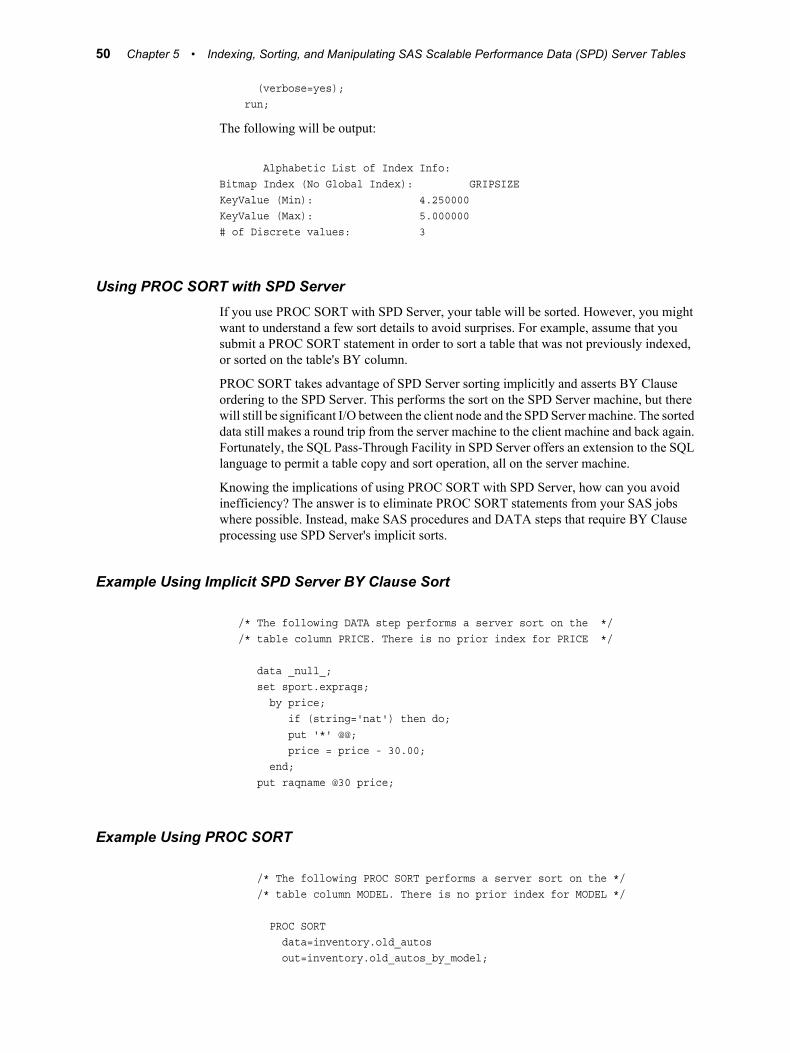
(verbose=yes); run;

The following will be output:

Alphabetic List of Index Info:Bitmap Index (No Global Index): GRIPSIZEKeyValue (Min): 4.250000KeyValue (Max): 5.000000# of Discrete values: 3

Using PROC SORT with SPD ServerIf you use PROC SORT with SPD Server, your table will be sorted. However, you mightwant to understand a few sort details to avoid surprises. For example, assume that yousubmit a PROC SORT statement in order to sort a table that was not previously indexed,or sorted on the table's BY column.

PROC SORT takes advantage of SPD Server sorting implicitly and asserts BY Clauseordering to the SPD Server. This performs the sort on the SPD Server machine, but therewill still be significant I/O between the client node and the SPD Server machine. The sorteddata still makes a round trip from the server machine to the client machine and back again.Fortunately, the SQL Pass-Through Facility in SPD Server offers an extension to the SQLlanguage to permit a table copy and sort operation, all on the server machine.

Knowing the implications of using PROC SORT with SPD Server, how can you avoidinefficiency? The answer is to eliminate PROC SORT statements from your SAS jobswhere possible. Instead, make SAS procedures and DATA steps that require BY Clauseprocessing use SPD Server's implicit sorts.

Example Using Implicit SPD Server BY Clause Sort

/* The following DATA step performs a server sort on the */ /* table column PRICE. There is no prior index for PRICE */

data _null_; set sport.expraqs; by price; if (string='nat') then do; put '*' @@; price = price - 30.00; end; put raqname @30 price;

Example Using PROC SORT

/* The following PROC SORT performs a server sort on the */ /* table column MODEL. There is no prior index for MODEL */

PROC SORT data=inventory.old_autos out=inventory.old_autos_by_model;


by model; run;

Example Using PROC SORT 51

Chapter 6Using SAS Scalable PerformanceData (SPD) Server with OtherClients

Overview . . . . . . . . . . . . . . . . . . . . . . . . . . . . . . . . . . . . . . . . . . . . . . . . . . . . . . . . . . . . 53

Using Open Database Connectivity (ODBC) to Access SPD Server Tables . . . . . . 54Why Use ODBC? . . . . . . . . . . . . . . . . . . . . . . . . . . . . . . . . . . . . . . . . . . . . . . . . . . . 54Installing OBDC Drivers on the Server . . . . . . . . . . . . . . . . . . . . . . . . . . . . . . . . . . 55Configuring ODBC on the Client . . . . . . . . . . . . . . . . . . . . . . . . . . . . . . . . . . . . . . . 55Preparing your Client Machine for ODBC Installation . . . . . . . . . . . . . . . . . . . . . . 56Two Types of ODBC Connections . . . . . . . . . . . . . . . . . . . . . . . . . . . . . . . . . . . . . 56Primary and Secondary LIBNAME Domains . . . . . . . . . . . . . . . . . . . . . . . . . . . . . 57Configuring an ODBC Data Source to Connect Directly to a SPD Server . . . . . . . 57Configuring an ODBC Data Source for SPD SNET . . . . . . . . . . . . . . . . . . . . . . . . 58Editing the Services File on Your Machine - ODBC Details . . . . . . . . . . . . . . . . . 58Creating a Query Using an ODBC-Compliant Program . . . . . . . . . . . . . . . . . . . . . 59

Using JDBC (Java) to Access SPD Server Tables . . . . . . . . . . . . . . . . . . . . . . . . . . . 59Why Would I Want to Use JDBC? . . . . . . . . . . . . . . . . . . . . . . . . . . . . . . . . . . . . . 59How Is JDBC Set Up on the Server? . . . . . . . . . . . . . . . . . . . . . . . . . . . . . . . . . . . . 60How Is JDBC Set Up on the Client? . . . . . . . . . . . . . . . . . . . . . . . . . . . . . . . . . . . . 60How Do I Use JDBC to Make a Query? . . . . . . . . . . . . . . . . . . . . . . . . . . . . . . . . . 60JDBC Code Examples and Tips . . . . . . . . . . . . . . . . . . . . . . . . . . . . . . . . . . . . . . . . 61Limitations of Using JDBC with SPD Server . . . . . . . . . . . . . . . . . . . . . . . . . . . . . 61

Using htmSQL to Access SPD Server Tables . . . . . . . . . . . . . . . . . . . . . . . . . . . . . . 62Why Would I Want to Use htmSQL? . . . . . . . . . . . . . . . . . . . . . . . . . . . . . . . . . . . 62How Is htmSQL Set Up on the Server? . . . . . . . . . . . . . . . . . . . . . . . . . . . . . . . . . . 63How Is htmSQL Set Up on the Client? . . . . . . . . . . . . . . . . . . . . . . . . . . . . . . . . . . 63How Do I Use htmSQL to Make a Query? . . . . . . . . . . . . . . . . . . . . . . . . . . . . . . . 63Examples of Setting Up an htmSQL Web Page . . . . . . . . . . . . . . . . . . . . . . . . . . . 64

Using SQL C API to Access SPD Server Tables . . . . . . . . . . . . . . . . . . . . . . . . . . . . 64Why Would I Want to Use SQL C API? . . . . . . . . . . . . . . . . . . . . . . . . . . . . . . . . . 64

OverviewThis chapter describes using SAS Scalable Performance Data (SPD) Server to connect withODBC, JDBC, htmSQL, and SQL C API clients.

Scalable Performance Data Server provides ODBC, JDBC, htmSQL, and SQL C APIaccess to SPD Server data stores from all supported platforms.

53

SPD Server can read tables exported from Base SAS software using PROC COPY, and,with the proper drivers installed on the network, allows queries on the tables from clientmachines that do not have SAS software.

There are four possible options:

• ODBC:Open Database Connectivity - This is an interface standard that provides acommon interface for accessing databases. Many software applications running in aWindows environment are compliant with this standard and can access data created byother software. This is a good choice if you have client machines running Windowsapplications, such as Microsoft Excel or Microsoft Access.

• JDBC:Java Database Connectivity - This option allows users with browsers to log onto a Web page and make a query. The results of the request are formatted and returnedto a Web page. This makes information available across a wide range of client platformsbecause all you need, after installing the JDBC driver on SPD Server, is a Web pagewith some Java code, and a client machine with a Java-enabled browser.

• htmSQL:HyperText Markup Structured Query Language - This option allows userswith browsers to log on to a Web page and make a query. The results of the request areformatted and returned to a Web page. This makes information available across a widerange of client platforms. Why? After installing the htmSQL driver in SPD Server, allyou need is an htmSQL Web page and a client machine with a browser.

• SQL C API:This option allows access to SPD Server tables from SQL statementsgenerated by C/C++ language applications. This access is provided in the form of a C-language run-time access library. This library provides a set of functions that you canuse to write custom applications to process SPD Server tables and to generate new ones.This library is designed to support multi-threaded applications and is available on allsupported SPD Server platforms.

Note: GUI interfaces might not display all return codes or error messages that the servergenerates.

Using Open Database Connectivity (ODBC) toAccess SPD Server Tables

Read this section if you do not have Base SAS software on the network client, but you wantto access SPD Server tables on the network, using an ODBC compliant program, such asMicrosoft Word, Query, Excel, or Access, and you have SPD Server tables available foruse, somewhere on the network, or SPD Server data servers and SPD Server snet serversrunning, or client machines in a Windows environment.

Why Use ODBC?You have SPD Server tables available on your network, and one or more of the followingmight be true:

• You do not have Base SAS software running on the Windows client, but you need toview or change SPD Server tables.

• You need to view or change the SPD Server tables using a Microsoft spreadsheet,database or word processor.

• You need to view or change SPD Server tables in ways that cannot be predeterminedor programmed into a Web page.

54 Chapter 6 • Using SAS Scalable Performance Data (SPD) Server with Other Clients

• You need to view or change SPD Server tables using Windows tools you are familiarwith.

Installing OBDC Drivers on the ServerInstructions for installing the OBDC driver are included in the SPD Server installationpackage.

Configuring ODBC on the Client1. Configure an ODBC data source.

2. Make your query using a Windows program.

Figure 6.1 Configure ODBC to Connect SPD Server Client to SPD Server Host

Configuring ODBC on the Client 55

Figure 6.2 Configure ODBC to Connect SPD Server Client to SPD SNET Server

Preparing your Client Machine for ODBC InstallationBefore you create OBDC data sources driver, you'll need the following information fromyour network administrator:

• a user name and password that is defined by a SPD Server administrator

• the primary LIBNAME domain of the SPD Server (also called the DBQ)

• the port number of the SPD name server (also called the SERV)

• the machine name or IP address of the SPD Server Name Server (also called the HOST)

• any secondary LIBNAME domains you want to assign to the ODBC connection.

Two Types of ODBC ConnectionsWith SPD Server software you can connect directly to a SPD Server without going throughthe SPD SNET server. Although connecting directly is the preferred method, connectionsvia the SPD snet server are still supported.

Note that connections via the SPD snet servers are not supported in the SAS 9 ODBCDriver software. If you intend to connect via the SPD snet Server you must install the SAS8 ODBC Driver.


Primary and Secondary LIBNAME DomainsWhen a connection to the SPD Server is established a primary LIBNAME domain isassigned. The primary LIBNAME domain is specified by the DBQ connection optionsparameter. Immediately after the connection is made the SAS ODBC Driver assigns thesecondary LIBNAME domains which are configured through the Libraries tab of the SASODBC Driver Configuration window.

ODBC Connections via the SPD snet server must have an odbc.parm file configured onthe SPD snet Server machine.

Configuring an ODBC Data Source to Connect Directly to a SPDServer

Once the SAS ODBC driver is installed, you will need to configure your ODBC data source.When you open the ODBC manager, you'll get a display screen that allows you to enterinformation that points the OBDC driver to the data on the SPD Server.

1. From the Windows Start button, select Start ð Settings ð Control Panel

2. Locate the ODBC Data Sources icon and open the Microsoft ODBC Data SourceAdministrator . The exact location of this program depends on your version ofWindows.

3. Select the Add button, then select the SAS ODBC driver.

4. Enter a data source name (and description if desired.)

5. Select the Servers panel and type in your two-part server name.

6. Click on the Configure box. The TCP Options window appears:

• Server Address: Enter the network address of the machine on which the SPDServer is running.

• Server User Name: Enter the user name as configured for a DBQ (SPD Serverprimary LIBNAME domain) on the SPD Server to which you will connect.

• Server User Password: Enter the user password as configured for a DBQ (SPDServer primary LIBNAME domain) on the SPD Server host to which you willconnect.

• Connection Options: Enter the Connection Options as follows:

• DBQ='SPD Server primary LIBNAME domain', this is the SPD ServerLIBNAME domain

• HOST='name server node name',this is the location of the host computer

• SERV='name server port number',this is the port number of the SPD Servername server running on the HOST.

• Any other SPD Server LIBNAME options. For more information, see the SPDServer 4.45: User's Guide section on “LIBNAME Options” on page 23.

7. Click OK, and then click Add, and select the Libraries panel.

8. Enter the DBQ name of a secondary LIBNAME domain in both the Name and HostFile text fields.

9. Enter spdseng in the Engine text field.

Configuring an ODBC Data Source to Connect Directly to a SPD Server 57

10. Follow the syntax rules for the SQL Pass-Through libref statement for entering a valuein the Options text field.

Configuring an ODBC Data Source for SPD SNETOnce the SAS ODBC driver is installed, you will need to configure your ODBC data source.When you open the ODBC manager, you'll get a display screen that allows you to enterinformation that points the OBDC driver to the data on the SPD Server.

1. From the Windows Start button, select Start ð Settings ð Control Panel

2. Click on the ODBC icon and select the Add button.

3. Select the SAS ODBC driver.

4. Enter a data source name (and description if desired).

5. Select the Servers panel and type in the two-part server name. The second part of theserver name should match the entry in the services file. In the example that follows thatshows you how to edit the services file, the server name is spdssnet.

6. Click on the Configure box. The TCP Options window appears with four input fieldsthat you fill:

• Server Address: Enter the network address of the machine on which the SPD snetserver is running.

• Server User Name: Enter the user name as configured for a DBQ (SPD Serverprimary LIBNAME domain) on the SPD Server to which you will connect.

• Server User Password: Enter the user password as configured for a DBQ (SPDServer primary LIBNAME domain) on the SPD Server host to which you willconnect.

• Connection Options: Enter the connection options as follows:

• DBQ='SPD Server primary LIBNAME domain':this is the SPD ServerLIBNAME domain.

• HOST='name server node name':this is the location of the host computer.

• SERV='name server port number':this is the port number of the SPD Servername server running on the HOST.

7. Click OK, and then click Add.

Editing the Services File on Your Machine - ODBC DetailsEditing the Services file is required only for ODBC connections via the SPD snet Server.

1. Find the Services file on your Windows machine. In Windows, the Services file isusually located in c:\windows\services

2. Open the Services file using a text editor.

3. The services file contains four columns. The rows of information can be sorted in portnumber order. Find the closest port number to the SPD Server port number, which youobtained from the network administrator (see “Preparing your Client Machine forODBC Installation ” on page 56). This is where you insert the new information.

4. Add an entry to the Services file, on its own line, in proper numeric order, using thefollowing syntax:


Table 6.1 How to Add Service Name and Port Number to the Services File

column1

<service name>

column2

<port number

& protocol>

column3

<aliases>

column4

<comment>

spdssnet

spdssnet=name

assigned to server

nnnn/tcp

nnnn=port number

protocol is

always /tcp

not

required

not

required

Remember: The service name, spdssnet must match the server name that you used in step6 of “Configuring an ODBC Data Source for SPD SNET ” on page 58. The port numbermust match the port number on which the SPD snet server is running.

Creating a Query Using an ODBC-Compliant ProgramThe following instructions create a query using Microsoft Access.

1. Start the SPD Server snet server.

2. Start Microsoft Access.

3. From the Microsoft Access main menu, select File ð Get External Table.

4. Select Link Table.

5. Select Files of Type.

6. Select ODBC Databases.

7. Select the data source.

Using JDBC (Java) to Access SPD Server TablesRead this information if you do not have Base SAS software on the network client, but youwant to use the power of the Java programming language to query SPD Server tables fromany client on the network that has a browser. You must have SPD Server tables on thenetwork and SPD Server and SPD snet servers running on the same server as the Webserver in order to use JDBC to access SPD Server tables.

Why Would I Want to Use JDBC?You might want to use JDBC if you have SPD Server tables available on your network andone or more of the following is true:

• You do not have Base SAS software on the network client to process the data sets.

• You want to distribute the information across your corporate intranet through a Webpage.

• The clients on your network are varied: UNIX boxes, Windows PCs, and workstations.One thing they might have in common is browser access to your intranet.

Why Would I Want to Use JDBC? 59

• The audience for the information understands Web browsing and wants point-and-clickaccess to the information.

• You want to distribute the information over the World Wide Web.

• Your planned application requires the power of the Java programming language.

How Is JDBC Set Up on the Server?JDBC is usually set up on the server at the time the SPD Server is installed. The processis covered in the SPD Server installation manual.

How Is JDBC Set Up on the Client?The client needs a browser set up to accept Java applets, such as

• Netscape Navigator, Release 3.0 or later

• Microsoft Internet Explorer, Release 3.02 or later.

How Do I Use JDBC to Make a Query?1. Log on to the World Wide Web and enter the URL for the Web page that contains the

JDBC code.

2. Click on the desired information.

3. JDBC handles the request, formats the information, and returns the result to the Webpage.


JDBC Code Examples and TipsThe following lines must be a part of the HTML file for JDBC:

<applet code=CLASSPATH.*.class codebase=../ width=600 height=425><param name=url value=jdbc:sharenet://spdssnet_node:PORT><param name=dbms_options value=DBQ='libname' HOST='host_node' SERV='NNNN'><param name=spdsuser value=userid><param name=sharePassword value=thepassword><param name=shareRelease value=V9><param name=dbms value=spds></applet>

Line 1:

• CLASSPATH points to the class path set up where the JDBC driver is installed.

• *.class is the name of the Java class that consumes all of the <PARAM name=...> lines.

Line 2:

• spdssnet_node is the node name of the machine on which the SPD snet server isrunning.

• PORT=port number of the machine on which the SPD snet server is running.

Line 3:

• value=DBQ='libref' is the LIBNAME domain of the SPD Server.

• HOST='host_node'is the location of the SPD snet server.

• SERV='NNNN'is the port number of the name server.

Line 4:

• spdsuser value=user ID is the user ID that queries the SPD Server table.

Line 5:

• sharePassword value=thepassword is the password of the user ID that will make thequery.

Line 6:

• shareRelease value=V9 is the version of the driver you are using. This must not bealtered.

Line 7:

• Sets the foreign database property on the JDBC driver. This means that the server isnot SAS and JDBC should not create a DataBaseMetaData object. See the examplesbelow for how to get around this.

Limitations of Using JDBC with SPD Server

JDBC Used with SAS Versus JDBC Used with SPD ServerSPD Server is treated as a foreign database. SPD Server clients can't query the JDBCmetadata class for available tables and other metadata. Users must write their own queriesto do this.

Limitations of Using JDBC with SPD Server 61

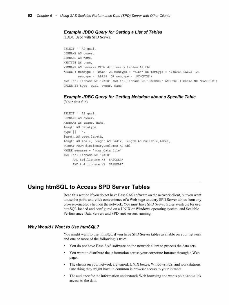
Example JDBC Query for Getting a List of Tables(JDBC Used with SPD Server)

SELECT '' AS qual,LIBNAME AS owner,MEMNAME AS name,MEMTYPE AS type,MEMNAME AS remarks FROM dictionary.tables AS tblWHERE ( memtype = 'DATA' OR memtype = 'VIEW' OR memtype = 'SYSTEM TABLE' OR memtype = 'ALIAS' OR memtype = 'SYNONYM')AND (tbl.libname NE 'MAPS' AND tbl.libname NE 'SASUSER' AND tbl.libname NE 'SASHELP')ORDER BY type, qual, owner, name

Example JDBC Query for Getting Metadata about a Specific Table(Your data file)

SELECT '' AS qual,LIBNAME AS owner,MEMNAME AS tname, name,length AS datatype,type || ' ',length AS prec,length,length AS scale, length AS radix, length AS nullable,label,FORMAT FROM dictionary.columns AS tblWHERE memname = 'your data file'AND (tbl.libname NE 'MAPS' AND tbl.libname NE 'SASUSER' AND tbl.libname NE 'SASHELP')

Using htmSQL to Access SPD Server TablesRead this section if you do not have Base SAS software on the network client, but you wantto use the point-and-click convenience of a Web page to query SPD Server tables from anybrowser-enabled client on the network. You must have SPD Server tables available for use,htmSQL loaded and configured on a UNIX or Windows operating system, and ScalablePerformance Data Servers and SPD snet servers running.

Why Would I Want to Use htmSQL?You might want to use htmSQL if you have SPD Server tables available on your networkand one or more of the following is true:


• You want to distribute the information across your corporate intranet through a Webpage.

• The clients on your network are varied: UNIX boxes, Windows PCs, and workstations.One thing they might have in common is browser access to your intranet.

• The audience for the information understands Web browsing and wants point-and-clickaccess to the data.


• You would like to use the JDBC option to extract the information but cannot permitJava applets to run on your network browsers.

• You want to distribute the information over the World Wide Web.

• Your developers are familiar with SQL and HTML.

How Is htmSQL Set Up on the Server?• htmSQL is usually set up on the server at the time the SPD Server is installed. The

process is covered in the SPD Server installation manual.

• htmSQL must be installed on the Web server and you need the name of a data sourcethat points to the SPD snet server and to the specific LIBNAME domain that containsthe SPD Server data you are interested in.

How Is htmSQL Set Up on the Client?HtmSQL requires nothing more than a browser on the network or Web client.

Figure 6.3 htmSQL Configured on a SPD Server Client

How Do I Use htmSQL to Make a Query?1. Log on to the World Wide Web and enter the URL for the Web page that contains the

htmSQL code.

2. Click on the desired information.

3. htmSQL handles the request, formats the information, and returns the result to the Webpage.

How Do I Use htmSQL to Make a Query? 63

Examples of Setting Up an htmSQL Web PageSAS Institute maintains a Web site that explains the technical details of setting up htmSQLWeb pages. In some cases, there are references to the SAS/SHARE product. The rules forsetting up htmSQL for either the SPD Server or SAS/SHARE are virtually the same.

The SAS Institute Web page for htmSQL is http://support.sas.com/rnd/web/intrnet/htmSQL/index.html.

Using SQL C API to Access SPD Server TablesRead this section if you do not have Base SAS software on the network client but you wantto provide your network client machines with the capability of accessing SPD Server tables,using SQL query methods. You must have SPD Server tables available for use, SPD Serversand SPD snet servers running, and Network client machines capable of running C/C++programs.

Why Would I Want to Use SQL C API?You have SPD Server tables available on your network and one or more of the followingmight be true:


• You want to distribute the information across your corporate intranet.

• The clients on your network are varied: UNIX boxes, Windows PCs, workstations. Onething they might have in common is the ability to run C/C++ programs.

• Your developers are familiar with SQL and C/C++.

“SAS Scalable Performance Data (SPD) Server SQL Access Library API Reference” onpage 159 contains additional information about SQL C API.


http://support.sas.com/rnd/web/intrnet/htmSQL/index.html

http://support.sas.com/rnd/web/intrnet/htmSQL/index.html

Chapter 7SAS Scalable Performance Data(SPD) Server Dynamic ClusterTables

Introduction to Dynamic Cluster Tables . . . . . . . . . . . . . . . . . . . . . . . . . . . . . . . . . . 65

Dynamic Cluster Table Structure . . . . . . . . . . . . . . . . . . . . . . . . . . . . . . . . . . . . . . . 66

Benefits of Dynamic Cluster Tables . . . . . . . . . . . . . . . . . . . . . . . . . . . . . . . . . . . . . . 67Overview of Dynamic Cluster Tables . . . . . . . . . . . . . . . . . . . . . . . . . . . . . . . . . . . 67Parallel Loading . . . . . . . . . . . . . . . . . . . . . . . . . . . . . . . . . . . . . . . . . . . . . . . . . . . . 67Fast and Economical Refreshes . . . . . . . . . . . . . . . . . . . . . . . . . . . . . . . . . . . . . . . . 67

Creating and Controlling Dynamic Cluster Tables . . . . . . . . . . . . . . . . . . . . . . . . . 68Create a Dynamic Cluster Table . . . . . . . . . . . . . . . . . . . . . . . . . . . . . . . . . . . . . . . 68Dynamic Cluster Table Access Control . . . . . . . . . . . . . . . . . . . . . . . . . . . . . . . . . 70Add Tables to a Dynamic Cluster . . . . . . . . . . . . . . . . . . . . . . . . . . . . . . . . . . . . . . 70Undo Dynamic Cluster Tables . . . . . . . . . . . . . . . . . . . . . . . . . . . . . . . . . . . . . . . . . 72Refresh Dynamic Cluster Tables . . . . . . . . . . . . . . . . . . . . . . . . . . . . . . . . . . . . . . . 74Modify Dynamic Cluster Tables . . . . . . . . . . . . . . . . . . . . . . . . . . . . . . . . . . . . . . . 75

Dynamic Cluster BY Clause Optimization . . . . . . . . . . . . . . . . . . . . . . . . . . . . . . . . 76Overview of Optimizing BY Clauses . . . . . . . . . . . . . . . . . . . . . . . . . . . . . . . . . . . . 76Dynamic Cluster BY Clause Optimization Example . . . . . . . . . . . . . . . . . . . . . . . 77

Member Table Requirements for Creating Dynamic Cluster Tables . . . . . . . . . . 79Overview of Table Requirements . . . . . . . . . . . . . . . . . . . . . . . . . . . . . . . . . . . . . . . 79Table Attributes . . . . . . . . . . . . . . . . . . . . . . . . . . . . . . . . . . . . . . . . . . . . . . . . . . . . 79Variable Attributes . . . . . . . . . . . . . . . . . . . . . . . . . . . . . . . . . . . . . . . . . . . . . . . . . . 80Index Attributes . . . . . . . . . . . . . . . . . . . . . . . . . . . . . . . . . . . . . . . . . . . . . . . . . . . . 81

Querying and Reading Member Tables in a Dynamic Cluster . . . . . . . . . . . . . . . . 82

Unsupported Features in Dynamic Cluster Tables . . . . . . . . . . . . . . . . . . . . . . . . . 83

Dynamic Cluster Table Examples . . . . . . . . . . . . . . . . . . . . . . . . . . . . . . . . . . . . . . . 84Create a Dynamic Cluster Table Example . . . . . . . . . . . . . . . . . . . . . . . . . . . . . . . . 84Add Tables to a Dynamic Cluster Example . . . . . . . . . . . . . . . . . . . . . . . . . . . . . . . 88Undo Dynamic Cluster Table Example . . . . . . . . . . . . . . . . . . . . . . . . . . . . . . . . . . 88Refresh Dynamic Cluster Table Example . . . . . . . . . . . . . . . . . . . . . . . . . . . . . . . . 88

Introduction to Dynamic Cluster TablesSPD Server is designed to meet the storage and performance demands that are associatedwith processing large amounts of data using SAS. As the size of the data grows, the demandto process that data increases, and storage architecture must change to keep up with businessneeds.

65

SPD Server offers dynamic cluster tables. Earlier releases of SPD Server provided a typeof cluster table called the time-based partitioning table. To optimize the benefits of theclustering, the SPD Server administrator can use dynamic clusters to partition SPD Serverdata tables for speed and enhanced I/O processing. Clustering is performed using metadatathat when combined with SPD Server functionality, provides parallel processingcapabilities for loading and querying data tables. Parallel processing can accelerateperformance and increase the manageability, flexibility, and scalability of very large datastores.

Dynamic Cluster Table StructureThe SPD Server dynamic cluster table can be considered as part of a hierarchy of tableswith increasing sophistication:

• Traditional SAS tablesare single files that contain the data descriptors and the tabledata. Data values are the columns, and the descriptors are the metadata that describethe column and data formatting that the table uses. If a traditional SAS table containsone or more indexes, they are stored in a separate file.

• SPD Server tablesuse component files to store tables. One component file stores thestream of data values. Another component file stores the column and data descriptors.If you create an index for a column or a composite of columns, SPD Server creates twoseparate component files (a *.hbx file and a *.idx file) for each index.

• SPD Server Cluster tablesare virtual table structures. SPD Server cluster tables consistof members. Each member is an SPD Server table. All members must share the samemetadata formats and organization. SPD Server cluster tables use the metadata tomanage the data that is contained in the members.

The SPD Server dynamic cluster table structure provides architecture that enablesflexible loading and rapid storage and processing for very large data tables. Usingdynamic cluster tables, loading data, removing data, and refreshing tables in very largedata marts become easier and more timely. Dynamic cluster tables provide

66 Chapter 7 • SAS Scalable Performance Data (SPD) Server Dynamic Cluster Tables

organizational features and performance benefits that traditional SAS tables and SPDServer tables do not have.

Benefits of Dynamic Cluster Tables

Overview of Dynamic Cluster TablesOrganizing SPD Server data into dynamic cluster tables creates an architecture thatsupports parallelism, enhanced data flexibility and manageability, and significantlyimproved speed in robust data warehousing environments that use large and very large datatables.

For example, you can add new data or remove historical data from very large tables byaccessing only the member tables that are affected by the change. You can access theindividual member tables in parallel. This strategy reduces the time that is needed for thejob to complete and uses simple commands. Furthermore, a complete refresh of a dynamiccluster table can occur using a fraction of the disk space that is needed to refresh a largetraditional SAS or SPD Server table that contains the same amount of data.

Parallel LoadingBecause dynamic cluster tables are virtual tables that consist of numerous small SPD Servertables, the architecture enables parallel loading and processing. Cluster table loads andrefreshes are broken down into multiple tasks that can be performed concurrently. SeparateSAS MP CONNECT jobs manage the parallel loading and processing.

The scalability of parallel loading with dynamic cluster tables depends on the scalabilityof the server I/O and the number of processors on the server.

Parallel loading requires multiple concurrent writes to disk. If the I/O hardware does notscale appropriately, the loading process can degrade performance.

SPD Server can create multiple indexes on the same table in parallel, and index creation isa CPU-intensive process.

When sufficient processing power is available, parallel index creation in SPD Server ishighly scalable.

The creation process for each index is multi-threaded. A single index creation can usemultiple CPUs on a server if they are available, which greatly improves performance.

Fast and Economical RefreshesRefreshing a dynamic cluster table requires only a fraction of the disk space that a traditionalSPD Server table with the same amount of data would require. The dynamic cluster tablearchitecture allows users to refresh many large tables concurrently, while conserving diskand I/O resources. With very large traditional SAS or SPD Server tables, available diskspace often limits the number of tables that can be concurrently refreshed.

In the life cycle of data warehouses, tables can be refreshed to recapture disk space whenrows have been updated or deleted, or to reorder data for optimized performance. However,refreshing a table can temporarily use twice the disk space of the table itself. With verylarge tables, disk space can be a limiting factor when updating a data warehouse or datamart. When disk space is limited on a server, the amount of data that can be refreshed at

Fast and Economical Refreshes 67

any given time is constrained. The window of time that is required to load and refresh canbecome huge.

Because dynamic cluster tables can be quickly unbound into smaller SPD Server tables,refreshing dynamic cluster tables does not use twice the disk space of the original table.Instead, only twice the disk space of the largest member table in the dynamic cluster tableis required.

After the dynamic cluster table is unbound, disk space equal to the first member table isrequired to perform a refresh. A backup of the refresh is created, and then the old versionis deleted, creating more available disk space. The refresh process repeats for eachsuccessive member table until all members in the dynamic cluster table have been refreshedand updated. Then, the member tables are merged into a dynamic cluster table once again.

When a server has enough disk space and I/O resources to refresh more than one membertable at a time, the benefits of parallel processing can be realized.

Creating and Controlling Dynamic Cluster TablesCreating dynamic cluster tables in SPD Server is simple and straightforward. The followingoperations are associated with creating and controlling dynamic cluster tables:

Create a Dynamic Cluster TableTo create dynamic cluster tables in SPD Server, you must have a set of related SPD Servertables that you want to cluster, such as tables that contain monthly sales histories. The SPDServer tables that you want to cluster must all be in the same domain, and must use identicaltable structures (columns and indexes) and compression. However, member table partitionsizes and member table owners can vary. These requirements ensure the metadatacompatibility that is necessary to create dynamic cluster tables in SPD Server.

Once the related SPD Server tables are organized, a simple PROC SPDO command is usedto bind the tables into a dynamic cluster table.

The following graphic represents a dynamic cluster table with 24 members. Each membertable is an SPD Server table that contains monthly sales transactions:


The following code shows the PROC SPDO command syntax that is used to create dynamiccluster tables from the member tables:

PROC SPDO library=domain-name ; cluster create Sales_History mem=sales200301 mem=sales200302 mem=sales200303 mem=sales200304 mem=sales200305 mem=sales200306 mem=sales200307 mem=sales200308 mem=sales200309 mem=sales200310 mem=sales200311 mem=sales200312 mem=sales200401 mem=sales200402 mem=sales200403 mem=sales200404 mem=sales200405 mem=sales200406 mem=sales200407 mem=sales200408 mem=sales200409 mem=sales200410 mem=sales200411 mem=sales200412 maxslot=36 ; quit ;

Create a Dynamic Cluster Table 69

PROC SPDO uses a LIBRARY statement to identify the domain that contains the tablesto be clustered. The cluster create syntax specifies the name of the dynamic cluster tableto be created (Sales_History).

The mem= syntax identifies the members of the cluster table. The tables in the previousexample represent monthly sales transactions. This example uses 24 monthly sales tablesfor the years 2003 and 2004.

The maxslot= specification specifies the maximum number of members that are allowedin the dynamic cluster table Sales_History.

The “Dynamic Cluster Table Examples ” on page 84 section contains more extensivecode examples of creating dynamic cluster tables.

Dynamic Cluster Table Access ControlA user must have SPD Server control access on any member tables that are used in theCLUSTER CREATE or CLUSTER ADD commands. A user must also have SPD Servercontrol access on the dynamic cluster table itself to submit a CLUSTER UNDO command.There is no restriction on table ownership, as long as the user has control access on allmember tables. All users that have access to a domain have default control access on tablesthat were created by the user Anonymous within that domain. ACLs can be defined on adynamic cluster table after it is created, and the permissions that are specified in thedynamic cluster table ACL are applied when SPD Server accesses the dynamic clustertable. Any individual ACL that is defined on a member table does not apply during thetime when the member table is part of a created dynamic cluster table.

Add Tables to a Dynamic ClusterTo add tables to a dynamic cluster table, you must have an existing dynamic cluster table.The SPD Server tables that you want to add to the dynamic cluster table must all be in thesame domain as the dynamic cluster table. These tables must use identical table structures(columns and indexes) and compression. However, partition sizes and owners can vary.These requirements ensure the metadata compatibility that is required to add to a dynamiccluster table.

Once the tables to be added are organized, a simple PROC SPDO command is used to addthe new tables to an existing dynamic cluster table. In the following graphic, sales tablesfor the first six months of 2005 are set up to be added to the dynamic cluster table thatcontains monthly sales transaction data for 2003 and 2004:


The following code shows the PROC SPDO command syntax that is used to add new tablesto an existing dynamic cluster table:

PROC SPDO library=domain-name ; cluster add Sales_History mem=sales200501 mem=sales200502 mem=sales200503 mem=sales200504 mem=sales200505 mem=sales200506 ; quit ;

PROC SPDO uses a LIBRARY statement to identify the domain that contains the existingdynamic cluster table that you want to add to. The cluster add syntax specifies the nameof the dynamic cluster table that you want to add to (Sales_History).

The mem= syntax identifies the members that form the table to be added to the existingdynamic cluster table. In the following graphic, six tables that include monthly salestransactions for the first half of 2005 are set up to be added to the existing dynamic clustertable of 2003 and 2004 sales transactions data:

Add Tables to a Dynamic Cluster 71

See the “Dynamic Cluster Table Examples ” on page 84 section for a more extensivecode example of adding to a dynamic cluster table.

Undo Dynamic Cluster TablesTo undo a dynamic cluster table, you must have an existing dynamic cluster table. Undoingthe dynamic cluster table simply reverts the table back to unbound SPD Server tables.Undoing a dynamic cluster table is required to remove a specific member table from adynamic cluster table, to add data to a specific member table in the dynamic cluster table,or to completely refresh a specific member table that belongs to the dynamic cluster table.

The following graphic represents a dynamic cluster table with 24 members. Each membercontains monthly sales transactions for the years 2003 and 2004:


PROC SPDO is used to undo the existing dynamic cluster table.

The following code shows the PROC SPDO command syntax that is used to undo anexisting dynamic cluster table:

PROC SPDO library= domain-name ; cluster undo Sales_History ; quit ;

PROC SPDO uses a LIBRARY statement to identify the domain that contains the existingdynamic cluster table that you want to undo. The cluster undo syntax specifies the nameof the dynamic cluster table that you want to undo (Sales_History).

The following graphic represents the previous dynamic cluster table, now unbound.

Undo Dynamic Cluster Tables 73

See the “Dynamic Cluster Table Examples ” on page 84 section for a more extensivecode example of undoing a dynamic cluster table and then refreshing it.

Refresh Dynamic Cluster TablesTo refresh a dynamic cluster table, you perform the same actions that are required to undoa dynamic cluster table. Then, you recreate the dynamic cluster table after you add amember table or change an existing member table. An example of refreshing an SPD Serverdynamic cluster table is updating on a monthly basis a dynamic cluster table whosemembers are the 24 previous months of sales transaction data.

To refresh a dynamic cluster table, use sequential PROC SPDO commands to UNDOCLUSTER and CREATE CLUSTER with the desired member tables. The dynamic clustertable is first undone. Table changes are made, and then the dynamic cluster table is reboundagain. The following example unbinds the sales transactions tables for 2003 and 2004, andthen refreshes the dynamic cluster table with sales transactions tables for the first six monthsof 2005:


See the “Dynamic Cluster Table Examples ” on page 84 section for a more extensivecode example of unbinding a dynamic cluster table and then refreshing it by recreating itwith different member tables.

Modify Dynamic Cluster TablesThe PROC SPDO command set for dynamic clusters provides a CLUSTER MODIFYcluster command. The usage syntax for the CLUSTER MODIFY command is

CLUSTER MODIFY clustername MINMAXVARLIST=(varname1 <varname2 varname3 ...>);

The CLUSTER MODIFY command sets a MINMAXVARLIST attribute on one or morevariables that belong to an existing dynamic cluster. The variable names that are specifiedin the CLUSTER MODIFY command must exist in the cluster and the variables must nothave a pre-existing MINMAXVARLIST setting. When the SPD Server runs the CLUSTERMODIFY command, the dynamic cluster is unclustered while the variable modificationsare made to the individual member tables. The cluster is recreated after theMINMAXVARLIST changes are completed. Control permission and exclusive access tothe dynamic cluster is required in order to run the CLUSTER MODIFY command. SPDServer performs a full table scan to initialize the MINMAXVARLIST values in eachmember table, so the processor time that is required to perform the CLUSTER MODIFYcommand is directly related to the size of the tables that belong to the cluster. If an erroroccurs while the CLUSTER MODIFY command is running, the cluster cannot be recreatedand the user will need to manually recreate the cluster using the CLUSTER CREATEcommand.

Modify Dynamic Cluster Tables 75

Dynamic Cluster BY Clause Optimization

Overview of Optimizing BY ClausesWhen you use SPD Server dynamic clusters, you can create huge data sets. If the huge datasets need further manipulation by some SAS job, it might be better to sort them for moreefficient processing. Traditional processing of huge data sets can overuse or overwhelmavailable resources. The resulting lack of available run-time or processor resources canprohibit you from running full-table scans and manipulating table rows, which are requiredto sort huge data sets for subsequent processing.

SPD Server provides dynamic cluster BY clause optimization to reduce the need for a largeamount of processor resources when evaluating BY clauses. The dynamic cluster BY clauseoptimization uses SPD Server to join individually created SPD Server member data setsso that the data sets appear to be single data set, while still keeping the individual memberdata sets intact. The dynamic cluster BY clause optimization uses the SORTEDBYmetadata of the member data sets to bypass most of the sorting that is required to performthe implicit BY clause ordering. With the SORTEDBY metadata of each member, SPDServer merges the member data sets in the dynamic cluster by using each member data set'sorder. No additional SPD Server work-space is required, and the ordered data set recordsare returned with minimum delay since member sorting is eliminated.

To use dynamic cluster BY clause optimization, you need to build the dynamic cluster tablea certain way. All of the member tables in your dynamic cluster table need to be sorted bythe same columns that you need to use in the BY clause. When you build your dynamiccluster table from member tables that are presorted by your BY clause columns, yourdynamic cluster table can use the BY clause optimization.

When a BY clause is run that matches the SORTEDBY column order of the dynamic clustertable member tables, SPD Server performs the BY clause without using sort work-spaceor experiencing first-record latency. SPD Server uses the presorted member tables toperform an instantaneous interleave. By using the presorted member tables, the dynamiccluster BY clause optimization enables you to perform operations on huge data sets thatwould be impossible to handle otherwise.

For example, suppose that you have a system that has sufficient CPU, memory, and work-space resources to sort a 50-GB data set in a reasonable amount of time. However, supposethis system accumulates 50 GB of new data every month, so that after 12 months, the datasets require 600 GB of storage. The system cannot handle sorting 600 GB of data to processqueries that are based on the previous 12-month period. If you use SPD Server to create adynamic cluster table from the 12 50-GB member tables, you can store each rolling monthof data in an SPD Server member table, and then sort it like the other dynamic cluster tablemember tables, and then add the new member table to the 600-GB dynamic cluster table.Now you can use the dynamic cluster BY clause optimization to run SAS steps that useBY clauses on the 600-GB cluster. For example, you can run a DATA step MERGEstatement that uses the dynamic cluster table as the master source for the MERGEstatement. The BY clause from the MERGE statement triggers the dynamic cluster BYclause optimization. As a result, the operation completes in the time that it takes tointerleave the individual member tables, using no SPD Server work-space and withoutexperiencing any implicit BY sort delays.

Dynamic cluster BY clause optimization allows the BY optimization to be combined withcertain WHERE clauses on dynamic cluster tables. For the WHERE clause optimizationto work, SPD Server must be able to determine whether the WHERE clause is trivially true


or trivially false for each member table in the dynamic cluster table. To be trivially true, aWHERE clause must find the clause condition true for every row in the member table. Tobe trivially false, a WHERE clause must find the clause condition false for every row inthe member table.

SPD Server keeps metadata about indexed values in dynamic cluster table member tables,and if the WHERE clause criteria can be determined as true or false based on the dynamiccluster table's member table metadata, the WHERE clause optimization is possible on amember-by-member basis for the entire dynamic cluster table. Suppose that member tablesof a dynamic cluster table all have an index on the column QUARTER (1=Jan-Mar, 2=Apr-Jun, 3=Jul-Sep, 4=Oct-Dec). Suppose that you need to run a DATA step MERGE statementthat uses the expression WHERE QUARTER=2. Because the QUARTER column isindexed in all of the member tables, SPD Server uses the BY clause optimization todetermine that the WHERE clause is trivially true. SPD Server then evaluates theexpression only on the member tables for April, May, and June without using any SPDServer work-space. When the WHERE clause can be determined as trivially true or triviallyfalse for each member table of the dynamic cluster table in advance, the BY clauseoptimization performs the BY processing only on the appropriate member tables.

The dynamic cluster BY clause optimization is triggered when member tables all have anapplicable SORTEDBY ordering for the BY clause that is asserted. When the SORTEDBYordering is strong (validated), SPD Server does not perform checks to verify the order ofBY variables that are returned from the member table. When the SORTEDBY ordering isweak (such as from a SORTEDBY assertion that was a data set option), additional checkingis performed to verify the order of BY variables that are returned from the member table.If an invalid BY variable order is detected, SPD Server terminates the BY clause anddisplays the following error message:

ERROR: Clustered BY member violates weak sort order during merge.

Dynamic Cluster BY Clause Optimization ExampleConsider a database of medical patient insurance claims, with quarterly claims data setsthat are named ClaimsQ1, ClaimsQ2, ClaimsQ3, and ClaimsQ4. Each quarterly claimstable is sorted by columns that are named PatID (for Patient ID) and ClaimID (for ClaimID). The member tables are combined into a dynamic cluster table that is named ClaimsAll.The following example shows the code:

DATA SPDS.ClaimsQ1;...run;

DATA SPDS.ClaimsQ2;...run;

PROC SORT DATA=SPDS.ClaimsQ1; BY PatID ClaimID;run;

PROC SORT DATA=SPDS.ClaimsQ2; BY PatID ClaimID;run;

PROC SPDO LIB=SPDS;

Dynamic Cluster BY Clause Optimization Example 77

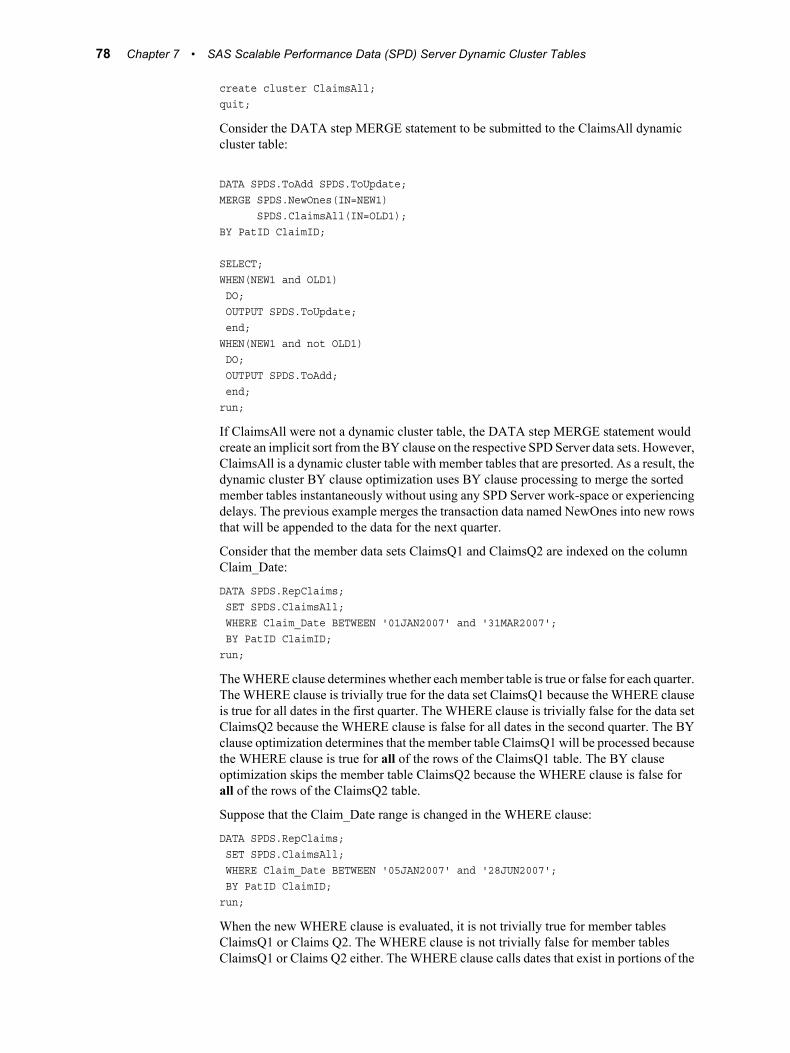
create cluster ClaimsAll;quit;

Consider the DATA step MERGE statement to be submitted to the ClaimsAll dynamiccluster table:

DATA SPDS.ToAdd SPDS.ToUpdate;MERGE SPDS.NewOnes(IN=NEW1) SPDS.ClaimsAll(IN=OLD1);BY PatID ClaimID;

SELECT;WHEN(NEW1 and OLD1) DO; OUTPUT SPDS.ToUpdate; end;WHEN(NEW1 and not OLD1) DO; OUTPUT SPDS.ToAdd; end;run;

If ClaimsAll were not a dynamic cluster table, the DATA step MERGE statement wouldcreate an implicit sort from the BY clause on the respective SPD Server data sets. However,ClaimsAll is a dynamic cluster table with member tables that are presorted. As a result, thedynamic cluster BY clause optimization uses BY clause processing to merge the sortedmember tables instantaneously without using any SPD Server work-space or experiencingdelays. The previous example merges the transaction data named NewOnes into new rowsthat will be appended to the data for the next quarter.

Consider that the member data sets ClaimsQ1 and ClaimsQ2 are indexed on the columnClaim_Date:

DATA SPDS.RepClaims; SET SPDS.ClaimsAll; WHERE Claim_Date BETWEEN '01JAN2007' and '31MAR2007'; BY PatID ClaimID;run;

The WHERE clause determines whether each member table is true or false for each quarter.The WHERE clause is trivially true for the data set ClaimsQ1 because the WHERE clauseis true for all dates in the first quarter. The WHERE clause is trivially false for the data setClaimsQ2 because the WHERE clause is false for all dates in the second quarter. The BYclause optimization determines that the member table ClaimsQ1 will be processed becausethe WHERE clause is true for all of the rows of the ClaimsQ1 table. The BY clauseoptimization skips the member table ClaimsQ2 because the WHERE clause is false forall of the rows of the ClaimsQ2 table.

Suppose that the Claim_Date range is changed in the WHERE clause:

DATA SPDS.RepClaims; SET SPDS.ClaimsAll; WHERE Claim_Date BETWEEN '05JAN2007' and '28JUN2007'; BY PatID ClaimID;run;

When the new WHERE clause is evaluated, it is not trivially true for member tablesClaimsQ1 or Claims Q2. The WHERE clause is not trivially false for member tablesClaimsQ1 or Claims Q2 either. The WHERE clause calls dates that exist in portions of the


member table ClaimsQ1, and it calls dates that exist in portions of the member tableClaimsQ2. The dates in the WHERE clause do not match all of the dates that exist in themember table ClaimsQ1, or all of the dates that exist in the member table ClaimsQ2. Thedates in the WHERE clause are not totally exclusive of the dates that exist in the membertables ClaimsQ1 or ClaimsQ2. As a result, BY clause optimization will not be used whenSPD Server runs the code.

Member Table Requirements for Creating DynamicCluster Tables

Overview of Table RequirementsWhen you create a dynamic cluster table, all of the member tables must have matchingtable, variable, and index attributes. If there are attribute mismatches, the dynamic clustertable creation fails, and SPD Server displays the following error message:

ERROR: Member table not compatible with other cluster members. Compare CONTENTS.

A more detailed error message is written to the SPD Server log. The SPD Server log listswhich attribute is mismatched in the member tables. The following lists specify the membertable attributes that must match for SPD Server to successfully create a dynamic clustertable.

• “Table Attributes ” on page 79

• “Variable Attributes ” on page 80

• “Index Attributes ” on page 81

Table AttributesThe following table attributes must match in all member tables to successfully create adynamic cluster table:

IDXSEGSIZEindex segment size

OBSLENobservation record length

NVARnumber of columns

NINDEXESnumber of indexes

DSORGdata set organization

SEMTYPEdata set semantic type

DSTYPESAS data set type

LOCALEcreation locale

Table Attributes 79

LANGdata set language tag

LTYPEdata set language type tag

FLAGScompressed data set

encrypted data set

backup data set

NLS variables in data set

minmaxvarlist variables in data set

SAS encryption password in data set

SASPWSAS encryption password

DS_ROLEdata set option for ROLE

ENCODING_CEIencoding CEI for NLS (for compressed tables)

DISKCOMPcompression algorithm

IOBLOCKSIZEI/O block size

IOBLOCKFACTORI/O block factor

Variable Attributes

The following variable attributes must match in all member tables to successfully create adynamic cluster table:

NAMEvariable name

LABELvariable label

NFORMvariable format

NIFORMvariable informat

NPOSvariable offset in record

NVAROvariable number in record

NLNGvariable length

NPRECvariable precision


FLAGSNLS encoding supported

minmaxvarlist variable

NFLformat length

NFDformat decimal places

NIFLinformat length

NIFDinformat precision

NSCALEscale for fixed-point decimal

NTATTRvariable type attributes

TYPEvariable type

SUBTYPEvariable subtype

SORTvariable sorted status

NTYPE2variable extended type code

Index Attributes

The following index attributes must match in all member tables to successfully create adynamic cluster table:

NAMEindex name

TYPEindex type

KEYFLAGSunique index

nomiss index

LENGTHindex length

NVARnumber of variables in index

NVAR0variable number in index

Index Attributes 81

Querying and Reading Member Tables in aDynamic Cluster

Dynamic clusters can be read using the MEMNUM= table option. The MEMNUM= optionenables you to perform query or read operations on a single member table that belongs toa dynamic cluster. When you use the MEMNUM= option, SPD Server opens only thespecified member table, instead of opening all of the member tables that belong to thecluster. You can determine the member number of a table in the cluster by issuing aCLUSTER LIST statement or a PROC CONTENTS command on the cluster. The SPDServer CLUSTER LIST or PROC CONTENTS command output lists the member tablesof the cluster in numbered order.

You can specify verbose output for the CLUSTER LIST statement by using the followingoption syntax:

CLUSTER LIST clustername [/VERBOSE]

When you issue the /VERBOSE option with a CLUSTER LIST statement, the output liststhe MINMAXVARLIST information for each member table in a dynamic cluster.

The following example uses PROC SPDO to create a dynamic cluster that has aMINMAXVARLIST on the numeric column STORE_ID of each member table. Then aCLUSTER LIST statement is issued using the /VERBOSE option. The CLUSTER LISToutput displays the dynamic cluster name, the names of each member table in the cluster,and the MINMAXVARLIST values for each member table.

PROC SPDO library=&libdom ;

CLUSTER CREATE ussales mem=ne_region mem=se_region mem=central_region maxslot=6 ;

CLUSTER LIST ussales/VERBOSE;MINMAXVARLIST COUNT = 1varname = store_idNumeric type.

Cluster Name USSALES, Mem=NE_REGION Variable Name (MIN,MAX) STORE_ID ( 1, 20)

Cluster Name USSALES, Mem=SE_REGION Variable Name (MIN,MAX) STORE_ID ( 60, 70)

Cluster Name USSALES, Mem=CENTRAL_REGION Variable Name (MIN,MAX) STORE_ID ( 60, 70)

NOTE: The maximum number of possible slots is 6.


You can specify an integer value n as an argument for the MEMNUM= table option toselect the nth member of the table, or you can use the argumentLASTCLUSTERMEMBER. When you use the LASTCLUSTERMEMBER argumentwith MEMNUM=, SPD Server selects the last member of the dynamic cluster table, withoutneeding to count the members to determine the number (n) of the last member.

The following example uses the MEMNUM= table option to query against the membertable sales200504 that belongs to the dynamic cluster table sales_history:

PROC SPDO library=&domain; ; CLUSTER CREATE sales_history mem=sales200501 mem=sales200502 mem=sales200503 mem=sales200504 mem=sales200505 mem=sales200506 maxslot=12 ; quit ;

PROC PRINT data=&domain..sales_history (MEMNUM=4); WHERE salesdate = 30Apr2005; run;

To use the MEMNUM= table option to query the last member table in the dynamic clustertable sales200506, the query would be:

PROC SPDO library=&domain ;

CLUSTER CREATE sales_history mem=sales200501 mem=sales200502 mem=sales200503 mem=sales200504 mem=sales200505 mem=sales200506 maxslot=12 ; quit ;

PROC PRINT data&domain..sales_history (MEMNUM=LASTCLUSTERMEMBER); WHERE salesdate = 15Jun2005; run;

Unsupported Features in Dynamic Cluster TablesBecause of differences in the load and read structures for dynamic cluster tables, somestandard features that are available in SAS tables and SPD Server tables are currently notsupported in SPD Server 4.5. These features are:

• You cannot append data to a dynamic cluster table. To append data to a dynamic clustertable, the table must be unclustered, the data is appended to the individual unclusteredfiles, and then the individual unclustered files must be reclustered.

• Record-level locking is not allowed.

Unsupported Features in Dynamic Cluster Tables 83

• The SPD Server backup/restore utility is not available.

• Copying data with PROC COPY or PROC SQL is not supported.

If a task for a dynamic cluster table requires one of these features, you should undo thedynamic cluster table and create standard SPD Server tables.

Dynamic Cluster Table ExamplesThe following four examples show all of the fundamental operations that are required touse dynamic cluster tables:

Create a Dynamic Cluster Table ExampleThe following example creates a dynamic cluster table named Sales_History. The first partof the example generates dummy transaction data that is used in the rest of the example.

The example uses SPD Server tables from the domain motorcycle. Twelve individual SPDServer tables for monthly motorcycle sales during 2004 are bound into the dynamic clustertable named Sales_History. Tables are created for the first six months of motorcycle salesduring 2005:

/* declare macro variables that will be used to *//* generate dummy transaction data */%macro var (varout,dist,card,seed,peak) ; %put &dist; &card; &seed; ; %local var1 ;

if upcase("&dist;") = 'RANUNI' then do ; &varout; = int(ranuni(&seed;)*&card;)+1; end ; else if upcase("&dist;") = 'RANTRI' then do ; *%let vartri = %substr("&dist;",5,2)&card; ; *&varout; = int(rantri(&seed;,&peak;)*&card;)+1; &varout; = int(rantri(&seed;,&peak;)*&card;)+1; end ;%mend ;

%macro linkvar (varin,varout,devisor) ; &varout; = int(&varin;/&devisor;) ;%mend ;

/* declare main vars */%let domain=motorcycle ;%let host=kaboom ;%let port=5200 ;%let spdssize=256M ;%let spdsiasy=YES ;

libname &domain; sasspds "&domain;" server=&host..;&port;


user='anonymous' ip=YES ;

/* generate monthly sales data tables for *//* 2004 and the first six months of 2005 */data &domain..sales200401; &domain..sales200402; &domain..sales200403; &domain..sales200404; &domain..sales200405; &domain..sales200406; &domain..sales200407; &domain..sales200408; &domain..sales200409; &domain..sales200410; &domain..sales200411; &domain..sales200412; &domain..sales200501; &domain..sales200502; &domain..sales200503; &domain..sales200504; &domain..sales200505; &domain..sales200506; ;

drop seed bump1 bump2 random_dist ;

seed = int(time()) ;

/* format the dummy transaction data */format trandate shipdate paiddate yymmdd10. ;

put seed ; do transact = 1 to 5000 ; %var (customer,ranuni,100000,seed,1) ;

%linkvar (customer,zipcode,10) ; %linkvar (customer,agent,20) ; %linkvar (customer,mktseg,10000) ; %linkvar (agent,state,100) ; %linkvar (agent,branch,25) ; %linkvar (state,region,10) ;

%var (item_number,ranuni,15000,seed,1) ;

%var (trandate,ranuni,577,seed,1) ; trandate = trandate + 16071 ;

%var (bump1,ranuni,20,seed,.1) ; shipdate = trandate + bump1 ;

%var (bump2,rantri,30,seed,.5) ; paiddate = trandate + bump2 ;

Create a Dynamic Cluster Table Example 85

%var (units,ranuni,100,seed,1) ; %var (trantype,ranuni,10,seed,1) ; %var (amount,rantri,50,seed,.5) ; amount = amount + 25 ;

random_dist = ranuni ('03feb2005'd) ;

/* sort the dummy transaction data into */ /* monthly sales data tables */

if '01jan2004'd <= trandate <= '31jan2004'd then output &domain..sales200401; ;

else if '01feb2004'd <= trandate <= '28feb2004'd then output &domain..sales200402; ;

else if '01mar2004'd <= trandate <= '31mar2004'd then output &domain..sales200403; ;

else if '01apr2004'd <= trandate <= '30apr2004'd then output &domain..sales200404; ;

else if '01may2004'd <= trandate <= '31may2004'd then output &domain..sales200405; ;

else if '01jun2004'd <= trandate <= '30jun2004'd then output &domain..sales200406; ;

else if '01jul2004'd <= trandate <= '31jul2004'd then output &domain..sales200407; ;

else if '01aug2004'd <= trandate <= '31aug2004'd then output &domain..sales200408; ;

else if '01sep2004'd <= trandate <= '30sep2004'd then output &domain..sales200409; ;

else if '01oct2004'd <= trandate <= '31oct2004'd then output &domain..sales200410; ;

else if '01nov2004'd <= trandate <= '30nov2004'd then output &domain..sales200411; ;

else if '01dec2004'd <= trandate <= '31dec2004'd then output &domain..sales200412; ;

else if '01jan2005'd <= trandate <= '31jan2005'd then output &domain..sales200501; ;

else if '01feb2005'd <= trandate <= '28feb2005'd then output &domain..sales200502; ;

else if '01mar2005'd <= trandate <= '31mar2005'd then output &domain..sales200503; ;


else if '01apr2005'd <= trandate <= '30apr2005'd then output &domain..sales200504; ;

else if '01may2005'd <= trandate <= '31may2005'd then output &domain..sales200505; ;

else if '01jun2005'd <= trandate <= '31jun2005'd then output &domain..sales200506; ; end ;run ;

/* index the transaction data in the *//* monthly sales data tables */%macro indexit (yrmth) ; PROC DATASETS library=&domain; nolist ; modify sales&yrmth; ; index create transact customer agent state branch trandate ; quit ;%mend ;

%let spdsiasy=YES ;

%indexit (200401) ;%indexit (200402) ;%indexit (200403) ;%indexit (200404) ;%indexit (200405) ;%indexit (200406) ;%indexit (200407) ;%indexit (200408) ;%indexit (200409) ;%indexit (200410) ;%indexit (200411) ;%indexit (200412) ;%indexit (200501) ;%indexit (200502) ;%indexit (200503) ;%indexit (200504) ;%indexit (200505) ;%indexit (200506) ;

/* Use PROC SPDO to create the dynamic cluster *//* table sales_history */PROC SPDO library=&domain; ; cluster create sales_history mem=sales200401 mem=sales200402 mem=sales200403 mem=sales200404 mem=sales200405 mem=sales200406 mem=sales200407 mem=sales200408

Create a Dynamic Cluster Table Example 87

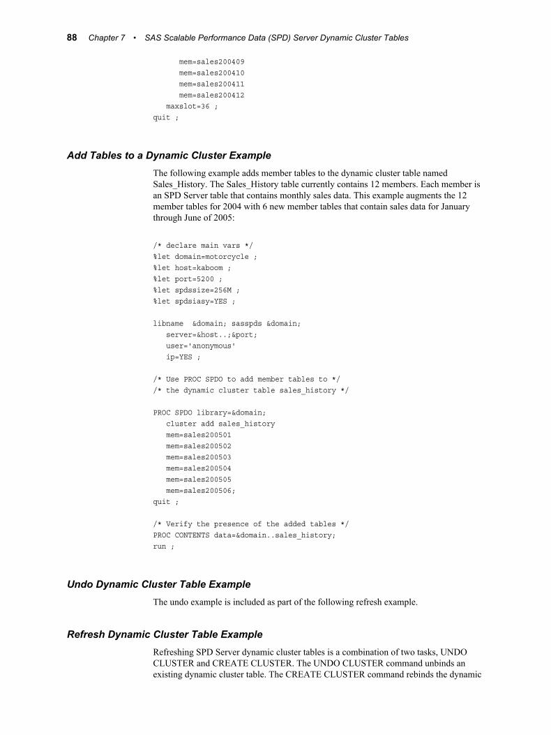
mem=sales200409 mem=sales200410 mem=sales200411 mem=sales200412 maxslot=36 ;quit ;

Add Tables to a Dynamic Cluster ExampleThe following example adds member tables to the dynamic cluster table namedSales_History. The Sales_History table currently contains 12 members. Each member isan SPD Server table that contains monthly sales data. This example augments the 12member tables for 2004 with 6 new member tables that contain sales data for Januarythrough June of 2005:


libname &domain; sasspds &domain; server=&host..;&port; user='anonymous' ip=YES ;

/* Use PROC SPDO to add member tables to *//* the dynamic cluster table sales_history */

PROC SPDO library=&domain; cluster add sales_history mem=sales200501 mem=sales200502 mem=sales200503 mem=sales200504 mem=sales200505 mem=sales200506;quit ;

/* Verify the presence of the added tables */PROC CONTENTS data=&domain..sales_history;run ;

Undo Dynamic Cluster Table ExampleThe undo example is included as part of the following refresh example.

Refresh Dynamic Cluster Table ExampleRefreshing SPD Server dynamic cluster tables is a combination of two tasks, UNDOCLUSTER and CREATE CLUSTER. The UNDO CLUSTER command unbinds anexisting dynamic cluster table. The CREATE CLUSTER command rebinds the dynamic


cluster table with updated member tables. Therefore, the following example shows boththe UNDO CLUSTER and CREATE CLUSTER commands with SPD Server dynamiccluster tables.

The following example refreshes the dynamic cluster table named Sales_History. TheSales_History table received additional member tables in the previous example. The 18-member dynamic cluster table Sales_History is unbound. The 12 member tables thatcontain 2004 sales data are deleted when the dynamic cluster table Sales_History isrecreated with only the six member tables that contain 2005 sales data. The combinedactions refresh the contents of the dynamic cluster table Sales_History.


libname &domain; sasspds &domain; server=&host..;&port; user='anonymous' IP=YES ;

/* Use PROC SPDO to undo the existing dynamic *//* cluster table Sales_History, then rebind *//* it with members from months in 2005 only */

PROC SPDO library=&domain; cluster undo sales_history ; cluster create sales_history mem=sales200501 mem=sales200502 mem=sales200503 mem=sales200504 mem=sales200505 mem=sales200506 maxslot=36 ;quit ;

/* Verify the contents of the refreshed dynamic *//* cluster table sales_history */

PROC CONTENTS data=&domain..sales_history;run ;

Refresh Dynamic Cluster Table Example 89

Part 3

SPD Server SQL Features

Chapter 8SPD Server SQL Features . . . . . . . . . . . . . . . . . . . . . . . . . . . . . . . . . . . . . . . . 93

91

Chapter 8SPD Server SQL Features

SPD Server SQL Planner . . . . . . . . . . . . . . . . . . . . . . . . . . . . . . . . . . . . . . . . . . . . . . . 94

Connecting to the SPD Server SQL Engine . . . . . . . . . . . . . . . . . . . . . . . . . . . . . . . . 95Implicit Pass-Through Connection . . . . . . . . . . . . . . . . . . . . . . . . . . . . . . . . . . . . . 95Explicit Pass-Through Connection . . . . . . . . . . . . . . . . . . . . . . . . . . . . . . . . . . . . . 95LIBNAME Syntax to Specify a Libref . . . . . . . . . . . . . . . . . . . . . . . . . . . . . . . . . . . 95Libref Statements . . . . . . . . . . . . . . . . . . . . . . . . . . . . . . . . . . . . . . . . . . . . . . . . . . . 96Libref Clauses . . . . . . . . . . . . . . . . . . . . . . . . . . . . . . . . . . . . . . . . . . . . . . . . . . . . . . 96Libref Examples . . . . . . . . . . . . . . . . . . . . . . . . . . . . . . . . . . . . . . . . . . . . . . . . . . . . 96

Specifying SPD Server SQL Planner Options . . . . . . . . . . . . . . . . . . . . . . . . . . . . . . 97Specify SQL Options using Explicit Pass-Through Code . . . . . . . . . . . . . . . . . . . . 97Specify SQL Options using Implicit Pass-Through Code . . . . . . . . . . . . . . . . . . . . 98

Important SPD Server SQL Planner Options . . . . . . . . . . . . . . . . . . . . . . . . . . . . . . 98_Method . . . . . . . . . . . . . . . . . . . . . . . . . . . . . . . . . . . . . . . . . . . . . . . . . . . . . . . . . . 98Reading the Method Tree . . . . . . . . . . . . . . . . . . . . . . . . . . . . . . . . . . . . . . . . . . . . . 99EXEC/NOEXEC . . . . . . . . . . . . . . . . . . . . . . . . . . . . . . . . . . . . . . . . . . . . . . . . . . 100MAGIC . . . . . . . . . . . . . . . . . . . . . . . . . . . . . . . . . . . . . . . . . . . . . . . . . . . . . . . . . . 101INDEXSELECTIVITY= . . . . . . . . . . . . . . . . . . . . . . . . . . . . . . . . . . . . . . . . . . . . 101OUTRSRTJNDX/NOOUTRSRTJNDX . . . . . . . . . . . . . . . . . . . . . . . . . . . . . . . . 101INOBS . . . . . . . . . . . . . . . . . . . . . . . . . . . . . . . . . . . . . . . . . . . . . . . . . . . . . . . . . . 102OUTOBS . . . . . . . . . . . . . . . . . . . . . . . . . . . . . . . . . . . . . . . . . . . . . . . . . . . . . . . . 102SASVIEW/NOSASVIEW . . . . . . . . . . . . . . . . . . . . . . . . . . . . . . . . . . . . . . . . . . . 102UNDO_POLICY= . . . . . . . . . . . . . . . . . . . . . . . . . . . . . . . . . . . . . . . . . . . . . . . . . 103BUFFERSIZE= . . . . . . . . . . . . . . . . . . . . . . . . . . . . . . . . . . . . . . . . . . . . . . . . . . . 103PRINTLOG/NOPRINTLOG . . . . . . . . . . . . . . . . . . . . . . . . . . . . . . . . . . . . . . . . . 104Additional SQL Reset Options . . . . . . . . . . . . . . . . . . . . . . . . . . . . . . . . . . . . . . . . 104

Parallel Join Facility . . . . . . . . . . . . . . . . . . . . . . . . . . . . . . . . . . . . . . . . . . . . . . . . . 105Overview of the Parallel Join Facility . . . . . . . . . . . . . . . . . . . . . . . . . . . . . . . . . . 105Parallel Join Methods . . . . . . . . . . . . . . . . . . . . . . . . . . . . . . . . . . . . . . . . . . . . . . 105Parallel Joins with Group-By . . . . . . . . . . . . . . . . . . . . . . . . . . . . . . . . . . . . . . . . . 106Parallel Join SQL Options . . . . . . . . . . . . . . . . . . . . . . . . . . . . . . . . . . . . . . . . . . . 106Parallel Join Example 1 . . . . . . . . . . . . . . . . . . . . . . . . . . . . . . . . . . . . . . . . . . . . . 107Parallel Join Example 2 . . . . . . . . . . . . . . . . . . . . . . . . . . . . . . . . . . . . . . . . . . . . . 107Parallel Join Example 3 . . . . . . . . . . . . . . . . . . . . . . . . . . . . . . . . . . . . . . . . . . . . . 108

Parallel Group-By Facility . . . . . . . . . . . . . . . . . . . . . . . . . . . . . . . . . . . . . . . . . . . . 108Overview of the Parallel Group-By Facility . . . . . . . . . . . . . . . . . . . . . . . . . . . . . . 108Enhanced Group-By Functions . . . . . . . . . . . . . . . . . . . . . . . . . . . . . . . . . . . . . . . . 109Table Aliases Supported . . . . . . . . . . . . . . . . . . . . . . . . . . . . . . . . . . . . . . . . . . . . . 109Nested Queries Meet Group-By Syntax Requirements . . . . . . . . . . . . . . . . . . . . . 109Formatted Parallel Group Select . . . . . . . . . . . . . . . . . . . . . . . . . . . . . . . . . . . . . . 110

93

Parallel Group-By SQL Options . . . . . . . . . . . . . . . . . . . . . . . . . . . . . . . . . . . . . . . 112GRPSEL/NOGRPSEL . . . . . . . . . . . . . . . . . . . . . . . . . . . . . . . . . . . . . . . . . . . . . . 112FMTGRPSEL/NOFMTGRPSEL . . . . . . . . . . . . . . . . . . . . . . . . . . . . . . . . . . . . . . 113SCANGRPSEL/NOSCANGRPSEL . . . . . . . . . . . . . . . . . . . . . . . . . . . . . . . . . . . 113

SPD Server STARJOIN Facility . . . . . . . . . . . . . . . . . . . . . . . . . . . . . . . . . . . . . . . 113

STARJOIN Options . . . . . . . . . . . . . . . . . . . . . . . . . . . . . . . . . . . . . . . . . . . . . . . . . . 114NOSTARJOIN . . . . . . . . . . . . . . . . . . . . . . . . . . . . . . . . . . . . . . . . . . . . . . . . . . . . 114STARMAGIC . . . . . . . . . . . . . . . . . . . . . . . . . . . . . . . . . . . . . . . . . . . . . . . . . . . . 114DETAILS . . . . . . . . . . . . . . . . . . . . . . . . . . . . . . . . . . . . . . . . . . . . . . . . . . . . . . . . 114

STARJOIN Facility Reference . . . . . . . . . . . . . . . . . . . . . . . . . . . . . . . . . . . . . . . . . 115Overview: SPD Server STARJOIN Facility . . . . . . . . . . . . . . . . . . . . . . . . . . . . . . 115Star Schemas . . . . . . . . . . . . . . . . . . . . . . . . . . . . . . . . . . . . . . . . . . . . . . . . . . . . . . 115SPD Server STARJOIN Requirements . . . . . . . . . . . . . . . . . . . . . . . . . . . . . . . . . 117Enabling STARJOIN Optimization in SPD Server . . . . . . . . . . . . . . . . . . . . . . . . 117Invoking the SPD Server STARJOIN Facility . . . . . . . . . . . . . . . . . . . . . . . . . . . . 117SPD Server STARJOIN Optimization . . . . . . . . . . . . . . . . . . . . . . . . . . . . . . . . . . 118Indexing Strategies to Optimize STARJOIN Query Performance . . . . . . . . . . . . . 121SPD Server STARJOIN RESET Statement Options . . . . . . . . . . . . . . . . . . . . . . . 124Example: STARJOIN RESET Statements . . . . . . . . . . . . . . . . . . . . . . . . . . . . . . . 125SPD Server STARJOIN Examples . . . . . . . . . . . . . . . . . . . . . . . . . . . . . . . . . . . . . 125

SPD Server Index Scan . . . . . . . . . . . . . . . . . . . . . . . . . . . . . . . . . . . . . . . . . . . . . . . 127

Optimizing Correlated Queries . . . . . . . . . . . . . . . . . . . . . . . . . . . . . . . . . . . . . . . . 130

Correlated Query Options . . . . . . . . . . . . . . . . . . . . . . . . . . . . . . . . . . . . . . . . . . . . 130_QRW/NO_QRW . . . . . . . . . . . . . . . . . . . . . . . . . . . . . . . . . . . . . . . . . . . . . . . . . 130_QRWENABLE/NO_QRWENABLE . . . . . . . . . . . . . . . . . . . . . . . . . . . . . . . . . 131

Materialized Views . . . . . . . . . . . . . . . . . . . . . . . . . . . . . . . . . . . . . . . . . . . . . . . . . . 132Materialized Views Operating Details . . . . . . . . . . . . . . . . . . . . . . . . . . . . . . . . . . 132User Interface for Materialized Views . . . . . . . . . . . . . . . . . . . . . . . . . . . . . . . . . 132Benefits of Materialized Views . . . . . . . . . . . . . . . . . . . . . . . . . . . . . . . . . . . . . . . 133Materialized View Example . . . . . . . . . . . . . . . . . . . . . . . . . . . . . . . . . . . . . . . . . 133

SPD Server SQL Extensions . . . . . . . . . . . . . . . . . . . . . . . . . . . . . . . . . . . . . . . . . . . 134BEGIN and END ASYNC OPERATION Statements . . . . . . . . . . . . . . . . . . . . . 134LOAD Statement . . . . . . . . . . . . . . . . . . . . . . . . . . . . . . . . . . . . . . . . . . . . . . . . . . 139COPY Statement . . . . . . . . . . . . . . . . . . . . . . . . . . . . . . . . . . . . . . . . . . . . . . . . . . 140

Differences between SAS SQL and SPD Server SQL . . . . . . . . . . . . . . . . . . . . . . 141Reserved Keywords . . . . . . . . . . . . . . . . . . . . . . . . . . . . . . . . . . . . . . . . . . . . . . . . 141Table Options and Delimiters . . . . . . . . . . . . . . . . . . . . . . . . . . . . . . . . . . . . . . . . . 141Mixing Scalar Expressions and Boolean Predicates . . . . . . . . . . . . . . . . . . . . . . . . 141INTO Clause . . . . . . . . . . . . . . . . . . . . . . . . . . . . . . . . . . . . . . . . . . . . . . . . . . . . . . 141Tilde Negation . . . . . . . . . . . . . . . . . . . . . . . . . . . . . . . . . . . . . . . . . . . . . . . . . . . . 141Nested Queries . . . . . . . . . . . . . . . . . . . . . . . . . . . . . . . . . . . . . . . . . . . . . . . . . . . . 142USER Value . . . . . . . . . . . . . . . . . . . . . . . . . . . . . . . . . . . . . . . . . . . . . . . . . . . . . . 142Supported Functions . . . . . . . . . . . . . . . . . . . . . . . . . . . . . . . . . . . . . . . . . . . . . . . . 142

SPD Server SQL PlannerSPD Server includes SQL Planner optimizations. SQL Planner optimizations improve theperformance of the more frequent query types that used in data mining solutions such asEnterprise Marketing Automation. A key enhancement to the SPD Server SQL Planner is

94 Chapter 8 • SPD Server SQL Features

optimizing correlated queries through the use of query rewrite techniques. Correlatedqueries are common in business and analytic intelligence data mining. Another significantenhancement is the tighter integration of the Parallel Group-By technology in the planner.The tighter integration adds performance benefits to nested Group-By syntax.

Connecting to the SPD Server SQL Engine

Implicit Pass-Through ConnectionYou can use an implicit pass-through connection to pass implicit SQL statements to theSPD Server SQL Engine. When you use an implicit pass-through connection, the SAS SQLplanner parses SQL statements to determine which, if any, portions can be passed to theSPD Server SQL Engine. In order for a submitted SQL statement to take advantage ofimplicit pass-through SQL, the tables that are referenced in the SQL statement must beSPD Server tables, and the SPD Server SQL engine must be able to successfully parse thesubmitted SQL statement.

An example of an SPD Server implicit pass-through connection is available in the Helpsection in this document on how to “Specify SQL Options using Implicit Pass-ThroughCode” on page 98.

Explicit Pass-Through ConnectionYou can use an explicit pass-through connection to pass explicit SQL statements to theSPD Server SQL Engine. When you use an explicit pass-through connection, you decideexplicitly which SQL statements are passed to the SPD Server SQL Engine. The explicitpass-through connection passes the entire SQL statement as written to the SPD Server SQLEngine, which parses and plans the SQL statement. All tables that are referenced in theSQL statement must be SPD Server tables or an error will occur.

An example of an SPD Server implicit pass-through connection is available in the Helpsection in this document on how to “Specify SQL Options using Explicit Pass-ThroughCode” on page 97.

LIBNAME Syntax to Specify a LibrefBelow is a LIBNAME statement that associates a libref, the SASSPDS engine, and an SPDServer domain.

LIBNAME librefSASSPDS <'SAS-data-library'> <SPD Server-options>;

Use the following arguments:

librefa name that is up to eight characters long and that conforms to the rules for SAS names.

SASSPDSthe name of the SPD Server engine.

'SAS-data-library'the logical LIBNAME domain name for an SPD Server data library on the host machine.The name server resolves the domain name into the physical path for the library.


LIBNAME Syntax to Specify a Libref 95

Libref StatementsWhenever you issue a CONNECT statement to an SPD Server SQL server with the DBQoption, by default you define a primary LIBNAME domain. The software uses the primarydomain to resolve table references in SQL statements executed for that connection.

You can also use the libref statement to assign secondary LIBNAME domains for the SPDServer SQL Server. The additional libref statements assign explicit LIBNAME domains,allowing the software to specify two-part table names for SQL statements executed for theconnection.

PROC SQL; execute(libref librefname <enginename> engopt= ' ')by sasspds;

Libref Clauses

The ENGNAME ClauseSpecifies the name of an alternate SAS I/O engine to service the libref's access to data. Ifyou do not specify an alternate SAS I/O engine, the default is spdseng, which accessesSPD Server tables.

The ENGOPT ClauseSpecifies options that configure the libref to access a specific data source or storage domain.Use single or double quotes around the clause. (If you have nested quotes within a clause,alternate between single and double quoted expressions.) The available options depend onthe current value of the ENGNAME option. For the default spdseng, you can specify anySPD Server CONNECT or LIBNAME engine option with the exception of prompt,newpasswd, and chngpass. Use the same keyword/value syntax required by theCONNECT statement.

Note: If you specify the SAS I/O engine spdseng and use explicit options in yourCONNECT statement, these options become default ENGOPT clause options. Explicitoptions can also be specified using the ENGOPT clause. Explicit options specified inan ENGOPT clause will override default values or declarations made in previousCONNECT statements.

Libref Examples

Libref for Another Domain but the Same CONNECT Statement UserIn this example the client connects to the SPD Server SQL server using the enginesasspds. The domain is mydomain, the server machine is called namesvrID, and the portnumber is namesvrPortNum. The execute statement assigns the libref cookie to anotherdomain, dough. After the libref is executed, the user issuing the connect statement can nowaccess either the default domain mydomain or the secondary domain dough.

PROC SQL; connect to sasspds


(dbq='mydomain' host='namesvrID' serv='namesvrPortNum' user='neraksr' passwd='siuya'); execute(libref cookie engopt=' dbq="dough"') by sasspds;

In the example above, the libref is cookie, and the secondary domain named is dough. Theintent of the example is to show how the CONNECT and libref statements work inconjunction to access multiple domains for the same user.

Libref to Same Domain but Different CONNECT Statement UserThis example assigns a libref to the domain specified by the CONNECT statement but foranother user (different SPD Server User ID).

PROC SQL; execute(libref samslib engopt=' user="sam" passwd="samspwd"') by sasspds;

Secondary Libref Using a Different HostThis example assigns a secondary libref to a different host machine.

PROC SQL; execute(libref sam2 engopt=' host="flex" dbq="samsplace"') by sasspds;

Specifying SPD Server SQL Planner OptionsThe SPD Server SQL Planner provides reset options that you can use to configure thebehavior of the SQL Planner and the SPD Server facilities that function through the SQLPlanner, such as the SPD Server Parallel Group-By facility, the SPD Server Parallel Joinfacility, and the SPD Server STARJOIN facility. You can specify SPD Server SQL resetoptions using either explicit pass-through or implicit pass-through code.

Specify SQL Options using Explicit Pass-Through CodeThe example below shows how to use an execute(reset <reset-options>) statement inexplicit SPD Server pass-through SQL code to invoke an SQL Planner, Parallel Group-Byfacility, Parallel Join facility, or STARJOIN facility reset option.

Most SQL Planner reset option usage examples in this document use explicit pass-throughcode. See the implicit pass-through code example below to see how SQL reset options can

Specify SQL Options using Explicit Pass-Through Code 97

be declared using an implicit %let spdssqlr= statement instead of an explicit execute(reset<reset-options>) statement.

/* Explicit Pass-Through SQL Example *//* to invoke an SQL Reset Option */

PROC SQL ;

connect to sasspds ( dbq=domain-name server=<host-name>.<port-number> user='username') ;

execute(reset <reset-options>) by sasspds ;

execute(SQL statements) by sasspds ;

disconnect from sasspds ; quit ;

Specify SQL Options using Implicit Pass-Through CodeThe example below shows how to use a %let spdssqlr=<reset-options> statement inimplicit SPD Server pass-through SQL code to invoke an SQL Planner, Parallel Group-Byfacility, Parallel Join facility, or STARJOIN facility reset option.

Most SQL Planner reset option usage examples in this document use explicit pass-throughcode. The implicit pass-through code example below shows how SQL reset options can bedeclared using an implicit %let spdssqlr= statement instead of an explicit execute(reset<reset-options>) statement.

/* Implicit Pass-Through SQL Example *//* to invoke an SQL Reset Option */

%let spdssqlr=<reset-options> ;

PROC SQL ;SQL statements ;

quit ;

Important SPD Server SQL Planner Options

_MethodThe SQL _method option is one of the most important reset options. The _method resetoption provides a method tree in the output that shows how the SQL was executed.

The following methods are displayed in the SQL _method tree:


sqxcrtaCreate table as Select.

sqxslctSelect rows from table.

sqxjslStep Loop Join (Cartesian Join).

sqxjmMerge Join execution.

sqxjndxIndex Join execution.

sqxjhshHash Join execution.

sqxsortSort table or rows.

sqxsrcRead rows from source.

sqxfilFilter rows from table.

sqxsumgSummary Statistics (with GROUP BY).

sqxsumnSummary Statistics (not grouped).

sqxuniqDistinct rows only.

sqxstjSTARJOIN

sqxxpgbParallel Group-By

sqxxpjnParallel Join with Group-By. The SAS log will display the name of the parallel joinmethod that was used.

sqxpllParallel Join without Group-By

Reading the Method TreeA method tree is produced in your output when the _methodreset option is specified forthe SQL Planner. The SQL Planner method tree is read from bottom row to top row. Belowis an example that shows how to interpret the method tree by substituting the type of methodthat was used in each step.

PROC SQL ;create table tbl1 as select * from path1.dansjunk1 a, path1.dansjunk2 b, path1.dansjunk3 c

Reading the Method Tree 99

where a.i = b.i and a.i = c.i ;quit ;

Here is the example Method Tree that was printed:

SPDS_NOTE: SQL execution methods chosen are:<0x00000001006BBD78> sqxslct<0x00000001006BBBF8> sqxjm<0x00000001006BBB38> sqxsort<0x0000000100691058> sqxsrc<0x0000000100667280> sqxjm<0x0000000100666C50> sqxsort<0x0000000100690BD8> sqxsrc<0x00000001006AE600> sqxsort<0x0000000100694748> sqxsrc

Reading from bottom to top, you can review the sequence of methods that were invoked.

SPDS_NOTE: SQL execution methods chosen are:<0x00000001006BBD78> step-9<0x00000001006BBBF8> step-8<0x00000001006BBB38> step7<0x0000000100691058> step-6<0x0000000100667280> step-5<0x0000000100666C50> step-4<0x0000000100690BD8> step-3<0x00000001006AE600> step-2<0x0000000100694748> step-1

In step 1, sqxsrc reads rows from the source. In step 2, sqxsort sorts the table rows. Thenin steps 3 and 4, more rows are read and sorted. In step 5, the tables are joined by sqxjm,and so on.

EXEC/NOEXECYou use the SPD Server SQL Planner EXEC/NOEXEC option to turn SPD Server SQLexecution on or off.

Usage:

/* This explicit Pass-Through SQL *//* prints the method tree without *//* executing the SQL code. */

PROC SQL ;connect to sasspds (dbq=domain server=<host-name>.<port-number> user='username') ;

execute (reset _method noexec) by sasspds ; /* turns SQL exec off */

execute (SQL statements) by sasspds ;


disconnect from sasspds ;quit ;

MAGICYou use the SPD Server SQL Planner MAGIC reset option that controls how the SPDServer SQL planner executes join statements. The Magic option has three settings, 101,102, and 103.

Usage:

execute(reset magic=<101/102/103>) by sasspds ;

MAGIC=101SPD Server performs sequential loop joins. Sequential loop joins are brute force joinsthat match every row from the first table to every row of the second table.

MAGIC=102SPD Server performs sort merge joins. Sort merge joins force a sort on all tables thatare involved in the join.

MAGIC=103SPD Server performs hash joins. Hash joins require SPD Server to create a memorytable in order to perform the join. The size of the memory table is limited based onmemory available.

INDEXSELECTIVITY=The INDEXSELECTIVITY= option allows you to tune SPD Server join methods,depending on the proportion of the tables to be joined. The index selectivity property canhave values of 0.0 or 1.0.

Usage:

execute(reset indexselectivity=<1.0/0.0>) by sasspds ;

INDEXSELECTIVITY=0.0 is the default SPD Server setting and uses index joinmethods.

INDEXSELECTIVITY=1.0 configures the SPD Server SQL planner to use a 15%heuristic rule when it decides to perform a join with an index. If the SPD Server SQLPlanner calculates that less than 15% of the total table rows will be selected in a join, theSQL Planner uses an index join method. If the SPD Server SQL Planner determines thatgreater than 15% of the total table rows will be selected in a join, the SQL Planner uses asort merge join.

OUTRSRTJNDX/NOOUTRSRTJNDXUse the OUTRSRTJNDX/NOOUTRSRTJNDX option to configure sort behavior for anSPD Server join index. OUTRSRTJNDX sorts the outer table for a join index by the joinkey. This is the default SPD Server setting. NOOUTRSRTJNDX does not sort the outertable for a join index.

OUTRSRTJNDX/NOOUTRSRTJNDX 101

Usage:

/* Disable outer table *//* sorting for a join index */execute(reset nooutrsrtjndx) by sasspds ;

/* Enable outer table *//* sorting for a join index */execute(reset outrsrtjndx) by sasspds ;

INOBSUse the INOBS option to specify the specific number of observations that you want to readfrom input tables.

Usage:

execute(reset inobs=<n>) by sasspds ;

where the integer value <n> is the desired number of observations.

OUTOBSUse the OUTOBS option to specify the specific number of observations that you want tocreate or print in your output.

Usage:

execute(reset outobs=<n>) by sasspds ;

where the integer value <n> is the desired number of observations.

SASVIEW/NOSASVIEWUse the SASVIEW/NOSASVIEW option to enable or disable SAS PROC SQL views thatuse an SPD Server LIBNAME. SAS PROC SQL views use a generic transport format torepresent numeric values, which SPD Server converts to native numeric values. Whenextremely large or extremely small numeric values are conveyed in a SAS PROC SQLview to SPD Server, some precision might be lost in extreme values during the SPD Servernumeric conversion.

Usage:

/* Disable SAS PROC SQL views *//* that use an SPD Server LIBNAME */execute(reset nosasview) by sasspds ;

/* Enable SAS PROC SQL views that *//* use an SPD Server LIBNAME */


execute(reset sasview) by sasspds ;

If SAS PROC SQL views are disabled and SPD Server Pass-Through SQL uses a viewthat was created by PROC SQL, SPD Server rejects the PROC SQL statement and insertsthe following error message in the SAS log::

SPDS_WARNING: SAS View and SASVIEW Reset Option equals No.SPDS_ERROR: An error has occured.

If SAS PROC SQL views are enabled and SPD Server Pass-Through SQL uses a view thatwas created by PROC SQL, SPD Server prints the following note in the SAS log:

SPDS_NOTE: SPDS using SAS View in transport mode.

UNDO_POLICY=Use the UNDO_POLICY option in SPD Server PROC SQL and RESET statements toconfigure SPD Server PROC SQL error recovery. When you update or insert rows in atable, you might receive an error message that states that the update or insert operationcannot be performed. The UNDO_POLICY option specifies how you want SPD Serverto handle rows that were affected by INSERT or UPDATE statements that preceded aprocessing error.

Usage:

/* Do not undo any updates or inserts */execute(reset undo_policy=none) by sasspds ;

/* Permit row inserts and updates to *//* be done up to the point of error */execute(reset undo_policy=required) by sasspds ;

UNDO_POLICY=NONEis the default setting for SPD Server. It does not undo any updates or inserts.

UNDO_POLICY=REQUIREDundoes all row updates or inserts up to the point of error.

UNDO_POLICY=OPTIONALUndoes any updates or inserts that it can undo reliably.

If the UNDO policy is not REQUIRED, you will get the following warning message foran insert into the table:

WARNING: The SQL option UNDO_POLICY=REQUIRED is not in effect. If anerror is detected when processing this insert statement, that errorwill not cause the entire statement to fail.

BUFFERSIZE=The SPD Server query optimizer considers a hash join when an index join is eliminated asa possibility. With a hash join, the smaller table is reconfigured in memory as a hash table.SQL sequentially scans the larger table and row-by-row performs a hash lookup againstthe small table to form the result set. On a memory-rich system, consider increasing the

BUFFERSIZE= 103

BUFFERSIZE= option to increase the likelihood that a hash join is chosen. The defaultBUFFERSIZE= setting is 64K. You can specify the amount of memory that you wantSPD Server to use for hash joins.

Usage:

/* Increase buffersize from 64K */execute(reset buffersize=1048576) by sasspds ;

PRINTLOG/NOPRINTLOGYou use the PRINTLOG/NOPRINTLOG option of the SPD Server SQL Planner to turnthe printing of the SQL statement text to the SPD Server log on or off.

Usage:

PROC SQL ;connect to sasspds (dbq=domain server=<host-name>.<port-number> user='username') ;

/* turn SQL statement printing on */execute (reset printlog)by sasspds ;

/* all statements will be printed to SPD Server log */execute (SQL statements)by sasspds ;

/* turn SQL statement printing off */execute (reset noprintlog)by sasspds ;

disconnect from sasspds ;quit ;

Additional SQL Reset OptionsMore detailed information about the available SQL reset options for the SPD Server SQLParallel Join, Parallel Group-By, STARJOIN, and Correlated Query facilities can be foundin this document as follows:

• “Parallel Join SQL Options ” on page 106

• “Parallel Group-By SQL Options ” on page 112

• “STARJOIN Options ” on page 114

• “Correlated Query Options ” on page 130


Parallel Join Facility

Overview of the Parallel Join FacilityThe Parallel Join facility is a feature of the SPD Server SQL planner that decreases therequired processing time when creating a pair-wise join between two SPD Server tables.The processing time savings is created when SPD Server performs the pair-wise join inparallel.

The SQL planner first searches for pairs when SPD Server source tables are to be joined.When a pair is found, the planner checks the join syntax for that pair to determine whetherit meets all of the requirements for the Parallel Join facility. If the join syntax meets therequirements, the pair of tables will be joined by the Parallel Join facility.

Parallel Join Methods

Parallel Sort-Merge MethodThe parallel sort-merge join method first performs a parallel sort to order the data, and thenmerges the sorted tables in parallel. During the merge, the facility concurrently joinsmultiple rows from one table with the corresponding rows in the other table. You can usethe parallel sort-merge join method to execute any join that meets the requirements forparallel join.

The parallel sort-merge method is a good all-around parallel join strategy that requires nointervention from the user. The tables for the sort-merge method do not need to be in thesame domain. The performance for the sort-merge method is not affected by the distributionof the data in the sort key columns.

The sort-merge method begins by completely sorting the smaller of the two tables beingjoined, while also performing concurrent partial parallel sorts on the larger table. If bothtables are very large and sufficient resources are not available to do the complete sort onthe smaller table, the performance of the parallel sort-merge method can degrade. Theparallel sort-merge method is also limited when performing an outer, left, or right join inparallel. Only two concurrent threads can be used when performing parallel outer, left, orright joins. Inner joins are not limited in the parallel sort-merge method and can use morethan two concurrent threads during parallel operations.

Parallel Range Join MethodThe parallel range join method uses a join index to determine the ranges of rows betweenthe tables that can be joined in parallel. The parallel range join method requires you tocreate a join index on the columns to be joined in the tables that you want to merge. Thejoin index divides the two tables into a specified number of near-equal parts, or ranges,based on matching values between the join columns. The Parallel Join Facility recognizesthe ranges of rows that contain matching values between the join columns, then usesconcurrent join threads to join the rows in parallel. The SPD Server parallel sort then sortsthe rows within a range.

The parallel range join method can be performed only on tables that are in the same domain.If either of the two tables are updated after the join index is created, the join index must berebuilt before the parallel range join method can be used. The parallel range join methodperforms best when the columns of the tables that are being joined are sorted. If the columns

Parallel Join Methods 105

are not relatively sorted, then the concurrent join threads can cause processor thrashing.Processor thrashing occurs when unsorted rows in a table require SPD Server to performincreasingly larger table row scans, which can consume processor resources at a high rateduring concurrent join operations.

More detailed information about creating join indexes is available in Chapter 17, "SASScalable Performance Data (SPD) Server Index Utility Ixutil," of the SAS ScalablePerformance Data (SPD) Server 4.5: Administrator's Guide.

How does the SPD Server Parallel Join facility choose between the sort-merge method andthe range join method? If a join index is available for the tables to be joined, the ParallelJoin facility will choose the parallel range join method. If a join index does not exist, or ifthe join index has not been rebuilt since a table was updated, the Parallel Join facilitydefaults to using the parallel sort-merge method.

Parallel Joins with Group-ByA powerful feature of the SPD Server Parallel Join facility is its integration with the SPDServer Parallel Group-By facility. If the result of the parallel join contains a group-bystatement, the partial results of the parallel join threads are passed to the Parallel Group-By facility, which performs the group-by operation in parallel. In the following example,SPD Server performs both a parallel join and parallel group-by operation.

LIBNAME path1 sasspds .... IP=YES;

PROC SQL;create table junk as select a.c, b.d, sum(b.e) from path1.table1 a, path1.table2 b where a.i = b.i group by a.d, b.d;quit;

When you use the SPD Server Parallel Join facility, you are not restricted to using theparallel group-by method only on single tables.

Parallel Join SQL Options

PLLJOIN/NOPLLJOINThe PLLJOIN/NOPLLJOIN option enables and disables the SPD Server Parallel Joinfacility.

Usage:

execute(reset noplljoin) by sasspds ; /* disables Parallel Join */

CONCURRENCYThe CONCURRENCY=<n> option sets the concurrency level that is used by the SPDServer Parallel Join facility, where the integer n specifies the number of levels. In mostcases, changing the default SPD Server concurrency setting (half of the available numberof processors) is not recommended.

Usage:


execute(reset concurrency=4) by sasspds ; /* enables 4 concurrency levels */

PLLJMAGICThe PLLJMAGIC option specifies how SPD server performs parallel joins.

Usage:

execute(reset plljmagic=<100/200>) by sasspds ;

PLLJMAGIC=100 forces a parallel range join when the range index is available.

PLLJMAGIC=200 forces a parallel merge join.

Parallel Join Example 1The first parallel join example is a basic SQL query that creates a pair-wise join of twoSPD Server tables, table1 and table2.


PROC SQL;create table junk as select * from path1.table1 a, path1.table2 b where a.i = b.i; quit;

Parallel Join Example 2The next parallel join example is an SQL query that uses more than two SPD Server tables.In this example, the SQL planner performs a parallel join on table1 and table2, and thenuse a non-parallel method to join the results of the first join and table3. A non-parallel joinmethod is used for the second join, because the criteria for a parallel join was not met. Aparallel join can be performed only on a pair-wise join of two SPD Server tables, and thequery calls three SPD Server tables.


PROC SQL;create table junk as select * from path1.table1 a, path1.table2 b, path1.table3 c where a.i = b.i and b.i = c.i;quit;

Parallel Join Example 2 107

Parallel Join Example 3Multiple parallel joins can be used in the same SQL query, as long as the SQL planner canperform the query using more than one pairwise join. In the next parallel join example, amore complex query contains a union of two separate joins. Both joins are pair-wise joinsof two SPD Server tables. There is a pair-wise join between table1 and table2, and then apair-wise join between table3 and table4 is performed concurrently, using the Parallel Joinfacility.

PROC SQL;create table junk as select * from path1.table1 a, path1.table2 b where a.i = b.i union

select * from path1.table3 c,path1.table4 dwhere c.i = d.i;quit;

The required criteria to use the SPD Server Parallel Join facility can be more complex thansimply requiring a pair-wise join of two SPD Server tables. The Parallel Join facility canhandle multiple character columns, numeric columns, or combinations of character andnumeric columns that are joined between pairs of tables. Numeric columns do not need tobe of the same width to act as a join key, but character columns must be of the same widthin order to be a join key. Columns that are involved in a join cannot be derived from a SASCASE statement, and cannot be created from character manipulation functions such asSUBSTR, YEAR, MONT, DAY, and TRIM.

Parallel Group-By Facility

Overview of the Parallel Group-By FacilitySPD Server SQL Planner optimizations improve the performance of the more frequentquery types used in data mining solutions. One of the SQL planner optimizations integratedinto SPD Server is tighter integration of the Parallel Group-By capability. Parallel Group-By is a high performance parallel summarization of data executed using SQL. ParallelGroup-By is often used in SQL queries (through the use of sub queries) to apply selectionlists for inclusion or exclusion. The tighter integration adds performance benefits to nestedGroup-By syntax.

Parallel Group-By looks for specific patterns in a query that can be performed using parallelprocessing summarization. Parallel Group-By works against single tables that are used toaggregate data. Parallel processing summarization is limited to the types of functions it canhandle.

The Parallel Group-By support in SPD Server has been expanded in many areas. ParallelGroup-By is integrated into the WHERE-clause planner code so that it will boost thecapabilities of the SPD Server SQL engine. Any section of code that matches the ParallelGroup-By trigger pattern will use it.


Enhanced Group-By FunctionsParallel Group-By now supports the following functions in syntax: COUNT, FREQ, N,USS, CSS, AVG, MEAN, MAX, MIN, NMISS, RANGE, STD, STDERR, SUM, VAR.These functions all can accept the DISTINCT term. The listed functions are the minimumsummary functions that are required in order to support the SAS Enterprise MarketingAutomation tool suite.

Table Aliases SupportedTable aliases are now supported in SPD Server in order to better support front end toolssuch as SAS Enterprise Marketing Automation. Tools such as SAS Enterprise MarketingAutomation generate SQL queries that use table aliases. Table aliases allow both shortercoding syntax and a method to select a specific column in a query that has two tables thatshare common column names.

Nested Queries Meet Group-By Syntax RequirementsSince the Parallel Group-By functionality is integrated into the SPD Server WHERE-clauseplanner, now many sections of queries can take advantage of performance enhancementssuch as parallel processing. Some common performance enhancements are sub-queries thatgenerate value lists in an IN clause, views that now conform to Parallel Group-By syntax,and views that contain nested Group-By syntax.

General Syntax:

SELECT 'project-list' FROM 'table-name' ;

WHERE [where-expression];

GROUP BY [groupby-list];

HAVING [having-expression];

ORDER BY [orderby-list];

project-listItems must be either column names (which must appear in the groupby-list) oraggregate (summary) functions involving a single column (with the exception ofcount(*) which accepts an asterisk argument. At least one aggregate function must bespecified. Project items can be aliased (for example, select avg(salary) as avgsal from )and these aliases can appear in any where-expression, having-expression, groupby-list or orderby-list. The following aggregate functions are supported: count, avg, avgdistinct, count distinct, css, max, min, nmiss, sum, sum distinct, supportc, range, std,stderr, uss, var. Mean is a synonym for avg. Freq and n are synonyms for count exceptthey do not accept the asterisk argument.

table-nameTable names can be one- or two-part identifiers (for example, mytable or foo.mytable),the latter requiring a previous libref statement to define the domain identifier (forexample, foo).

The where-expression is optional.

The optional groupby-list must be column names or projected aliases.

The optional having-expression must be a Boolean expression composed of aggregatefunctions, group by columns and/or constants.

Nested Queries Meet Group-By Syntax Requirements 109

The optional orderby-list must be projected column names or aliases or numbers whichrepresent the position of a projected item (for example, select a, count (*) order by 2).

Since the Parallel Group-By functionality is integrated into the SPD Server WHERE-clauseplanner, now many sections of queries can take advantage of performance enhancementssuch as parallel processing. Some common performance enhancements are sub-queries thatgenerate value lists in an IN clause, views that now conform to Parallel Group-By syntax,and views that contain nested Group-By syntax.

Formatted Parallel Group SelectBy default, the columns of a group-by statement are grouped by their unformatted value.SQL pass-through parallel group by provides the capability to also group data by thecolumns output data format. For example, you could group by the date column of a tablewith an input format of mmddyy8 and an output format of monname9. Suppose the columnhas dates 01/01/04 and 01/02/04. Grouping by the unformatted value would put these datesinto two separate groups. However, grouping by the formatted month name, would putthese values into the same month grouping of January.

You enable or disable pass-through formatted parallel group by with the following executecommands:

PROC SQL; connect to sasspds (dbq=........);

/* turn on formatted parallel group-by */ execute(reset fmtgrpsel) by sasspds;

select * from connection to sasspds (select dte from mytable groupby dte);

/* turn off formatted parallel group-by */ execute(reset nofmtgrpsel) by sasspds;

select * from connection to sasspds (select dte from mytable groupby dte);

quit;

The example code below is extracted from a larger block of code, whose purpose is to makecomputations based on user-defined classes of age, such as Child, Adolescent, Adult, andPensioner. The code uses SQL Parallel Group-By features to create the user-defined classesand then uses them to perform aggregate summaries and calculations.

/* Use the parallel group-by feature with the */


/* fmtgrpsel option. This groups the data based *//* on the output format specified in the table. *//* This will be executed in parallel. */

PROC SQL;connect to sasspds (dbq="&domain" serv="&serv" host="&host" user="anonymous");

/* Explicitly set the fmtgrpsel option */

execute(reset fmtgrpsel) by sasspds;

title 'Simple Fmtgrpsel Example'; select * from connection to sasspds (select age, count(*) as count from fmttest group by age);

disconnect from sasspds; quit;

PROC SQL;connect to sasspds (dbq="&domain" serv="&serv" host="&host" user="anonymous");



title 'Format Both Columns Group Select Example';

select * from connection to sasspds (select GENDER format=$GENDER., AGE format=AGEGRP., count(*) as count from fmttest formatted group by GENDER, AGE);

disconnect from sasspds;

quit;

PROC SQL;connect to sasspds (dbq="&domain" serv="&serv"

Formatted Parallel Group Select 111

host="&host" user="anonymous");



title1 'To use Format on Only One Column With Group Select'; title2 'Override Column Format With a Starndard Format';

select * from connection to sasspds (select GENDER format=$1., AGE format=AGEGRP., count(*) as count from fmttest formatted group by GENDER, AGE);


quit;

/* A WHERE-clause that uses a format to subset */ /* data is pushed to the server. If it is not */ /* pushed to the server, the following warning */ /* message will be written to the SAS log: */ /* WARNING: Server is unable to execute the */ /* where clause. */

data temp; set &domain..fmttest; where put (AGE,AGEGRP.) = 'Child'; run;

For the complete code example, see “User-Defined Formats Example” on page 271.

Parallel Group-By SQL OptionsSPD Server provides the following Parallel Group-By SQL reset options:

GRPSEL/NOGRPSELThe GRPSEL/NOGRPSEL option enables or disables the SPD Server Parallel Group-Byfacility.

Usage:

/* Disable Parallel Group-By */execute(reset nogrpsel) by sasspds ;


FMTGRPSEL/NOFMTGRPSELThe FMTGRPSEL/NOFMTGRPSEL option enables or disables the SPD Server ParallelGroup-By use of formats.

Usage:

/* Disable Parallel Group-By *//* use of formats. */execute(reset nofmtgrpsel) by sasspds ;

SCANGRPSEL/NOSCANGRPSELUse the SCANGRPSEL/NOSCANGRPSEL option to turn the SPD Server index scanfacility on and off. The default SPD Server setting uses the index scan facility.

Usage:

/* Disable index scan facility */execute(reset noscangrpsel) by sasspds ;

/* Enable index scan facility */execute(reset scangrpsel) by sasspds ;

SPD Server STARJOIN FacilityThe SPD Server's enhanced SQL planner includes the STARJOIN facility. The SPD ServerSTARJOIN facility validates, optimizes, and executes SQL queries on data that isconfigured in a star schema. Star schemas consist of two or more normalized dimensiontables that surround a centralized fact table. The centralized fact table contains dataelements of interest derived from the dimension tables.

In data warehouses with large numbers of tables and millions or billions of rows of data,properly constructed star joins can minimize overhead data redundancy during queryevaluation. If the SPD Server STARJOIN facility is not enabled, or of SPD Server SQLdoes not detect a star schema, then the SQL will be processed using pair-wise joins.

How do star joins differ from pair-wise joins? In SPD Server 4.4, properly configured starjoins require only three steps to complete, regardless of the number of dimension tables.SPD Server pair-wise joins require one step for each table to complete the join. If a starschema consisted of 25 dimension tables and one fact table, the STARJOIN is accomplishedin three steps; joining the tables in the star schema using pair-wise joins will require 26steps.

When data is configured in a valid SPD Server star schema, and the STARJOIN facility isnot disabled, the SPD Server STARJOIN facility can produce quicker and more processor-efficient SQL query performance than would be realized using SQL pair-wise join queries.

For more information about the STARJOIN Facility, see “STARJOIN Facility Reference”on page 115.

SPD Server STARJOIN Facility 113

STARJOIN OptionsUse the SPD Server SQL STARJOIN facility options to specify how SPD Serverimplements Star Joins.

NOSTARJOINUse the NOSTARJOIN option to disable or enable the SPD Server STARJOIN facility.

Usage

execute(reset nostarjoin=<1/0>) by sasspds ;

NOSTARJOIN=0 enables the SPD Server STARJOIN facility.

NOSTARJOIN=1 disables the SPD Server STARJOIN facility.

STARMAGICUse the STARMAGIC option to modify the behavior of the SPD Server STARJOIN andoverride some internal heuristics in order to favor a particular join strategy in the planner.The values are bit flags in the STARJOIN code that can be added together to result in avariety of controls.

Usage

execute(reset starmagic=<1/2/4/8/16>) by sasspds ;

STARMAGIC=1 forces all dimension tables to be classified as Phase I tables.

STARMAGIC=2 is currently not used.

STARMAGIC=4 requires an exact match on the FACT composite index in order to meetPhase I conditions for STARJOIN.

STARMAGIC=8 disables the IN-SET STARJOIN strategy. The IN-SET strategy isenabled by default.

STARMAGIC=16 disables the COMPOSITE STARJOIN strategy. The COMPOSITEstrategy is enabled by default.

DETAILSUse the DETAILS option to print details about your SPD Server STARJOIN facilitysettings. All internal STARJOIN debugging information is tied to the stj$ DETAILS key.Issuing the stj$ reset option displays available information as SPD Server attempts tovalidate a join sub-tree. The RESET DETAILS="stj$" option is very useful for debuggingSTARJOIN and SQL statement execution.

Usage

execute(reset details="stj$") by sasspds ;


STARJOIN Facility Reference

Overview: SPD Server STARJOIN FacilitySPD Server provides an enhanced SQL planner that includes the STARJOIN facility. TheSPD Server STARJOIN facility validates, optimizes, and executes SQL queries on datathat is configured in a star schema. Star schemas consist of two or more normalizeddimension tables that surround a centralized fact table. The centralized fact table containsdata elements of interest that are derived from the dimension tables.

In data warehouses with large numbers of tables and millions or billions of rows of data,a properly constructed STARJOIN can minimize overhead data redundancy during queryevaluation. If the SPD Server STARJOIN facility is not enabled, or if SPD Server SQLdoes not detect a star schema, then the SQL will be processed using pairwise joins.

How does a STARJOIN differ from a pairwise join? In SPD Server, a properly configuredSTARJOIN requires only three steps to complete, regardless of the number of dimensiontables. SPD Server pairwise joins require one step for each table to complete the join. If astar schema consists of 25 dimension tables and one fact table, the STARJOIN isaccomplished in three steps; joining the tables in the star schema using pairwise joinsrequires 26 steps.

When data is configured in a valid SPD Server star schema, and the STARJOIN facility isnot disabled, the SPD Server STARJOIN facility can produce quicker and more processor-efficient SQL query performance than SQL pairwise joins.

Star Schemas

Overview of Star SchemasTo exploit the power of the SPD Server STARJOIN facility, the data must be configuredas a star schema, and it must meet specific SPD Server SQL star schema requirements.

Star schemas are the simplest data warehouse schema, consisting of a central fact table thatis surrounded by multiple normalized dimension tables. Fact tables contain the measuresof interest. Dimension tables provide detailed information about the attributes within eachdimension. The columns in fact tables are either foreign key columns that define the linksbetween the fact table and individual dimension tables, or they are columns that calculatenumeric values that are based on foreign key data.

Figure 1 is an example of a simple star schema. The dimension tables Products, Supplier,Location, and Time surround the fact table Sales.

Star Schemas 115

Figure 8.1 Example Star Schema

The dimension tables, fact table, and keys in Figure 1 are used in the examples in thisdocument.

Dimension Tables InformationProducts is a table of products, with one row per unique product SKU. The row for eachunique SKU contains information such as product name, height, width, depth, weight, palletcube, and so on. The example Products table contains 1,500 rows.

Supplier is a table of the suppliers that supply the products. The row for each unique suppliercontains information such as supplier name, address, state, contact representative, and soon. The example Supplier table contains 25 rows.

Location is a table of the stores selling the products. The row for each unique locationcontains information such as store number, store name, store address, store manager, storesales volume, and so on. The Location table contains 500 rows.

Time is a sequential sales transaction table. Each row in the Time table represents one dayout of a rolling three-year, 365-day-per-year calendar. The row for each day containsinformation such as date, day of week, month, quarter, year, and so on. The Time tablecontains 1,095 rows.


Fact Table InformationThe fact table Sales is a table that combines information from the four dimension tables,Products, Supplier, Location, and Time. Its foreign keys are imported, one from eachdimension table: PRODUCT_CODE from Products, STORE_NUMBER from Location,SUPPLIER_ID from Supplier, and SALES_DATE from Time. The fact table Sales mighthave other columns with facts or information that are not found in any dimension table.Examples of fact table columns that are not foreign keys from a dimension table are columnssuch as QTY_SOLD or NET_SALES. The fact table in this example could contain as manyas 1,500 x 25 x 500 x 1,095 = 20,531,250,000 rows.

SPD Server STARJOIN RequirementsFor SPD Server SQL to take advantage of the STARJOIN planner, the following conditionsmust be true:

• STARJOIN optimization must be enabled in SPD Server.

• The SPD Server star schema must use a single central fact table.

• All dimension tables in the SPD Server star schema must be connected to the fact table.

• SPD Server dimension tables can appear in only one join condition.

• SPD Server fact tables are equally joined to dimension tables.

• SPD Server SQL infers fact tables by topology (common equally joined predicates).

• Dimension tables that have no subsetting require a simple index on the dimension table'sjoin column.

When SPD Server SQL is submitted that does not meet these STARJOIN conditions, SPDServer reverts to performing the requested SQL task using SPD Server's pairwise joinstrategy. The “SPD Server STARJOIN Examples” on page 125 section of this documentprovides three examples that show valid, invalid, and restricted candidates for the SPDServer STARJOIN facility.

Enabling STARJOIN Optimization in SPD ServerSPD Server STARJOIN optimization is enabled by default. The “SPD Server STARJOINRESET Statement Options” on page 124 section provides detailed information aboutstatement options that enable or disable the STARJOIN facility in SPD Server.

Invoking the SPD Server STARJOIN FacilitySPD Server knows when to use the STARJOIN facility because it is topology based. SPDServer invokes STARJOIN based on the SQL that is submitted. When SQL is submittedand STARJOIN optimization is enabled, SPD Server checks the submitted SQL foradmissible STARJOIN patterns. SPD Server SQL identifies a fact table by scanning for acommon equally joined table among multiple join predicates in a WHERE clause. WhenSPD Server SQL detects patterns that have multiple equally joined operators sharing acommon table, the common table becomes the star schema's fact table.

When an SQL statement that is submitted to SPD Server uses structures that indicate thepresence of a star schema, the STARJOIN validation checks begin.

Invoking the SPD Server STARJOIN Facility 117

SPD Server STARJOIN Optimization

Overview of STARJOIN OptimizationThe SPD Server STARJOIN optimization process searches for the most efficient SQLstrategy to use for computations. The STARJOIN optimization process consists of threesteps, regardless of the number of dimension tables that are joined to the fact table in thestar schema.

1. Classify dimension tables that are called by SQL as Phase I tables or Phase II tables.

2. Phase I probes fact table indexes and selects a STARJOIN strategy.

3. Phase II performs index lookups and joins subsetted fact table rows with Phase II tables.

Classify Dimension Tables That Are Called by SQL as Phase I Tablesor Phase II TablesAfter the STARJOIN planner validates the join sub-tree, join optimization begins. Joinoptimization is the process that searches for the most efficient SQL strategy to use whenjoining the tables in the star schema.

The first step in optimization is to examine the dimension tables that were called by SQLfor structures that SPD Server can use to improve performance. Each dimension table isclassified as a Phase I table or a Phase II table. The structure of a dimension table andwhether the submitted SQL filters or subsets the table's contents determine its classification.SPD Server uses different processes to handle Phase I and Phase II dimension tables.

Phase I tables can improve performance. A Phase I table is a dimension table that is eithervery small (nine rows or less), or a dimension table whose SQL queries contain one or morefiltering criteria that is expressed with a WHERE clause. A Phase II table is any dimensiontable that does not meet Phase I criteria. Rows in Phase II tables that are referenced in theSQL query are not subsetted.

Consider the star schema that is illustrated in Figure 8.1 on page 116, with the fact tableSales and the dimension tables Products, Supplier, Location, and Time.

Suppose a submitted SQL query requests transaction reports from the fact table Sales forall stores where the location is the state of North Carolina, for the time period of the monthof January, for all products, and for all suppliers. The SQL query subsets the Location andTime tables, so SPD Server classifies the Location and Time tables as Phase I tables. Thequery requests information from all of the rows in the Product and Supplier tables. Becausethose tables are not subsetted by a WHERE clause in the submitted SQL, STARJOINclassifies the Products and Supplier tables in this query as Phase II tables.

Now, using the same star schema, add more detail to the SQL query. Set up a new querythat requests transaction reports from the fact table Sales for all stores where the locationis the state of North Carolina, for the time period of the month of January, and for productswhere the supplier is from the state of North Carolina. The subsetted dimension tablesLocation, Time, and Supplier are classified as Phase I tables. The Products table, unfilteredby the submitted SQL query, is classified as a Phase II table.

Dimension tables are classified as Phase I or Phase II tables because the two types of tablesrequire different index probe methods.

Phase I Probes Fact Table Indexes and Selects a STARJOIN StrategyPhase I uses the SQL join keys from the subsetted Phase I dimension tables to get a smallerset of candidate rows to query in the central fact table. After optimizing the candidate rowsin the fact table, the Phase I index probe examines index structures to determine the best


STARJOIN strategy to use. There are two SPD Server STARJOIN strategies: the IN-SETstrategy and the COMPOSITE strategy. In all but a few cases, the IN-SET strategy is themost robust and efficient processing strategy. The user can determine which strategy SPDServer will choose by providing the required table index types in the submitted SQL.

Phase I creates the smaller set of candidate rows in the central fact table by eliminating facttable rows that do not match the SQL join keys from the subsetted Phase I dimension tables.For example, if the SQL query requests information about transactions that occurred onlyin North Carolina store locations, the candidate rows that are retained in the fact table willuse the SQL that subsets the Location dimension table:

WHERE location.STATE = "NC";

If the Sales fact table contains sales records for all 50 states, Phase I uses the SQL thatsubsets the Location dimension table to eliminate the sales records of all stores in statesother than North Carolina from the fact table candidate rows. The example is simple, butpowerful -- reducing the fact table candidate row set to transactions from only NorthCarolina stores eliminates massive amounts of nonproductive data processing.

The Phase I index probe inventories the number and types of indexes on the fact table anddimension tables as it attempts to identify the best STARJOIN strategy. To use theSTARJOIN IN-SET strategy, Phase I must find simple indexes on all SQL join columnsin the fact table and dimension tables. Otherwise, to use the STARJOIN COMPOSITEstrategy, Phase I searches for the best composite index that is available on the fact table.The best composite index for the fact table is the composite index that spans the largest setof join predicates from the aggregated Phase I dimension tables.

Based on the fact table and dimension table index probe, SPD Server selects the STARJOINstrategy using the following logic:

• If one or more simple indexes are found on fact table and dimension table SQL joincolumns, and no spanning composite indexes are found on the fact table, SPD Serverselects the STARJOIN IN-SET strategy.

• If an optimal spanning composite index is found on the fact table, and no simple indexesare found on fact table and dimension table SQL join columns, SPD Server selects theSTARJOIN COMPOSITE strategy.

• If both simple and spanning composite indexes are found, SPD Server generally selectsthe STARJOIN IN-SET strategy, unless the composite index is an exact match for allof the Phase I join predicates, and only lesser matches are available with the IN-SETstrategy.

• If no suitable indexes are found for either STARJOIN strategy, SPD Server does notuse STARJOIN; it joins the sub-tree using the standard SPD Server pairwise join.

The IN-SET and COMPOSITE join strategies have some underlying differences.

The IN-SET join strategy uses an IN-SET transformation of dimension table metadata toproduce a powerful compound WHERE clause to be used on the STARJOIN fact table.The "IN" part of the term "IN-SET" refers to an IN specification in the SQL WHEREclause. The IN-SET is the set of values that populate the contents of the SQL IN queryexpression. For example, in the following SQL WHERE clause, the cities Raleigh, Cary,and Clayton are the values of the IN-SET:

WHERE location.CITY in ("Raleigh", "Cary", "Clayton");

For the IN-SET strategy, Phase I dimension tables are subsetted, and then the resulting setof join keys form the SQL IN expression for the fact table's corresponding join column.You must have simple indexes on all SQL join columns in both the fact table and dimensiontables before STARJOIN Phase I can select the IN-SET strategy.

SPD Server STARJOIN Optimization 119

If the dimension table Location has six rows for Raleigh, Cary, and Clayton, then sixSTORE_NUMBER values are applied to the IN-SET WHERE clause that is used to selectthe candidate rows from the central fact table. The STARJOIN IN-SET facility transformsthe dimension table's CITY values into STORE_NUMBER values that can be used to selectcandidate rows from the Sales fact table. The transformed WHERE clause to be applied tothe fact table might resemble the following code:

WHERE fact.STORE_NUMBER in (100,101,102,103,104,105,106);

You can use IN-SET transformations in a star schema that has any number of dimensiontables and a fact table. Consider the following example dimension table subsettingstatement:

WHERE location.CITY in("Raleigh","Cary","Clayton") and Time.SALES_WEEK = 1;

Because the Sales fact table has no matching CITY column to join with the Locationdimension table, and no matching SALES_WEEK column to join with the Time table, theIN-SET strategy uses transformations to create a WHERE clause that the Sales fact tablecan resolve:

WHERE fact.STORE_NUMBER in (100,101,102,103,104,105,106)and Time.SALES_DATE in ('01JAN2005'd,'02JAN2005'd,'03JAN2005'd, '04JAN2005'd,'05JAN2005'd,'06JAN2005'd, '07JAN2005'd,);

The advantage of the STARJOIN facility is that it handles all of the transformations on afact table, from dimension table subsetting to IN-SET WHERE clauses.

The COMPOSITE join strategy uses a composite index on the fact table to exhaustivelyprobe the full Cartesian product of the combined join keys that is produced by theaggregated dimension table subsetting. SPD Server compares the composite indexes on thefact table to the theoretical composite index that is made from all of the join keys in thePhase I dimension tables. Phase I selects the best composite index on the fact table, basedon the join requirements of the dimension tables.

A disadvantage of using the COMPOSITE join strategy is that when more than a few joinkeys exist, the Cartesian product map can become large geometric matrixes that caninterfere with processing performance. You must have a composite index on the fact tablethat consists of Phase I dimension table join columns before STARJOIN Phase I can selectthe COMPOSITE join strategy.

If any Phase I dimension tables contain join predicates that do not have supporting simpleor composite indexes on the fact table, those Phase I dimension tables are dropped fromPhase I processing and are moved to the Phase II group.

Phase II Performs Index Lookups and Joins Subsetted Fact TableRows with Phase II TablesPhase I optimizes the join strategies between the Phase I dimension tables and the candidaterows from the fact table . After Phase I terminates, Phase II takes over. Phase II completesthe indicated joins between the candidate rows from the fact table and the correspondingrows in the subsetted Phase I dimension tables. After completing the joins with the PhaseI dimension tables, Phase II performs index lookups from the fact table to the Phasedimension II tables. Phase II dimension tables should have indexes created on all columnsthat join with the fact table.


When SPD Server completes the STARJOIN Phase I and Phase II tasks, the STARJOINoptimizations have been performed, the STARJOIN strategy has been selected, and thesubsetted dimension tables and fact table joins are ready to run and produce the desiredSQL results set.

Indexing Strategies to Optimize STARJOIN Query Performance

Overview of Indexing StrategiesOnce the baseline criteria to create an SQL STARJOIN in SPD Server have been satisfied,you can configure indexing to influence which strategy the SPD Server STARJOIN facilitychooses.

With the IN-SET strategy, the SPD Server STARJOIN facility can use multiple simpleindexes on the fact table. The IN-SET strategy is the simplest to configure, and usuallyprovides the best performance. To configure your work to choose the STARJOIN IN-SETstrategy, create a simple index on each fact table and dimension table SQL column thatyou want to use in a join relation. Creating simple indexes prevents STARJOIN Phase Ifrom rejecting a Phase I dimension table so that it becomes a non-optimized Phase II table.In addition, simple indexes facilitate the Phase II fact-table-to-dimension-table join lookup.

Consider the following SQL code for a star schema with one fact table and two dimensiontables:

PROC SQL;select F.FID, D1.DKEY, D2.DKEYfrom fact F, DIM1 D1, DIM2 D2where D1.DKEY EQ F.D1KEYand D2.DKEY EQ F.D2KEYand D1.REGION EQ 'Midwest'and D2.PRODUCT EQ 'TV';

Indexing to Optimize the IN-SET Join StrategyThe SPD Server IN-SET join strategy is the preferred strategy for almost every STARJOIN.If you want the previous example code to trigger the IN-SET STARJOIN strategy, createsimple indexes on the join columns for the star schema's fact table and dimension tables:

• On the fact table F, create simple indexes on columns F.D1KEY and F.D2KEY.

• On the dimension tables D1 and D2, create simple indexes on columns D1.DKEY andD2.DKEY.

Other fact table and dimension table indexes might exist that could filter WHERE clauses,but those simple indexes are the indexes that are needed to enable the STARJOIN IN-SETjoin strategy.

Indexing to Optimize the COMPOSITE Join StrategyUsing the COMPOSITE join strategy, the dimension tables with WHERE clause subsettingare collected from the set of equally joined predicates. A fact table composite index isneeded for the fact table columns that correspond to the subsetted dimension table columns.The composite index on the fact table is necessary to facilitate the dimension tables'Cartesian product probes on the fact table rows. The STARJOIN optimizer code looks forthe best composite index, which is based on the best and simplest left-to-right match of thecolumns in the COMPOSITE join.

If the subsetting in a STARJOIN is limited to a single dimension table, then theCOMPOSITE join strategy can be enabled by creating a simple index on the join columnof the single dimension table. That index is used to perform the Phase II index lookup on

Indexing Strategies to Optimize STARJOIN Query Performance 121

the fact table candidate rows. The fact table candidate row set is the result of the Phase Icomposite index probe.

For the previous example code to trigger the COMPOSITE STARJOIN strategy, create acomposite index named COMP1 on the fact table for each of the dimension table keys:F.COMP1=(D1KEY D2KEY).

Other fact table and dimension table indexes might exist that could filter WHERE clauses,but the COMPOSITE index named COMP1 is the type of index that is needed to enablethe STARJOIN COMPOSITE join strategy.

Although the COMPOSITE join strategy might appear to be a simpler configuration, thestrongest utility of the COMPOSITE join strategy is limited to join relations between thefact table and dimension tables that are based on a Cartesian matrix of outcomes. As thenumber of dimension tables and join relations increases, the resulting Cartesian matrixesincrease geometrically in size and can become unmanageable. The superior performanceof the IN-SET strategy is so dramatic and robust that you should consider using theCOMPOSITE join strategy only if you have good evidence that it compares favorably withthe IN-SET strategy.

Example: Indexing using the IN-SET Join StrategyThe example star schema in Figure 8.1 on page 116 has four dimension tables (Supplier,Products, Location, and Time) and one fact table (Sales) with simple indexes on theSUPPLIER_ID, PRODUCT_CODE, STORE_NUMBER, and SALES_DATE columns inthe Sales fact table.

Consider the following SQL query to create a January sales report for an organization'sNorth Carolina stores:

PROC SQL;select sum(s.sales_amt) as sales_amt sum(s.units_sold) as units_sold s.product)code, t.sales_month

from spdslib.sales s, spdslib.supplier sup, spdslib.products p, spdslib.location l, spdslib.time t

where s.store_number = l.store_numberand s.sales_date = t.sales_dateand s.product_code = p.product_codeand s.supplier_id = sup.supplier_idand l.state = 'NC'and t.sales_date between '01JAN2005'd and '31JAN2005'd;

quit;

During optimization, the STARJOIN planner examines the WHERE clause subsetting inthe SQL to determine which dimension tables qualify as Phase I tables and which are PhaseII tables.


The WHERE clause subsetting of the STATE column of the Location dimension table(where ... l.state = 'NC') and the subsetting of the SALES_DATE column of the Timedimension table (where ... t.sales_date between '01JAN2005'd and '31JAN2005'd)cause SPD Server to process the Location and Time tables as Phase I tables. The remainingdimension tables Supplier and Products are processed as Phase II tables.

SPD Server STARJOIN uses the Phase I dimension tables to reduce the rows in the facttable to candidate rows that contain the matching criteria. The values in each dimensiontable key are used to create a list of values that meet the subsetting criteria of the fact table.

For example, the previous SQL query is intended to create a January sales report for storeslocated in North Carolina. Note that the WHERE clause in the SQL code joins the Locationand Sales tables on the STORE_NUMBER column. Suppose that there are 10 unique NorthCarolina stores, with consecutively ordered STORE_NUMBER values that run from 101to 110. When the WHERE clause is evaluated, the results will include a list of the 10 NorthCarolina store IDs that existed in January 2005.

With simple indexes on the fact table and dimension tables for the STORE_NUMBERcolumn, STARJOIN chooses the IN-SET strategy. Subsetting the STATE column valuesto 'NC' allows STARJOIN to build the set of store numbers that are associated with NorthCarolina locations. STARJOIN can use the set of North Carolina store numbers to generatea where ... in SQL expression. SQL uses the where ... in expression to efficiently subsetthe candidate rows in the fact table before the final SQL expression evaluation.

In other words, STARJOIN uses a matrix of database relationships and index combinationsto reorganize the SQL expression for more internal processing that can take advantage ofthe IN-SET join strategy. For the previous example code, the internal STARJOIN SQLreorganization resembles the following example code. The WHERE clause IN-SETstatements for the STORE_NUMBER and TIME columns can be rapidly processed tosubset the candidate rows in the Sales fact table. (The optimized code sections arehighlighted.)

PROC SQL; select sum(s.sales_amt) as sales_amt sum(s.units_sold) as units_solds.product)code, t.sales_month

from spdslib.sales s, spdslib.supplier sup, spdslib.products p, spdslib.location l, spdslib.time t

where s.store_number = l.store_number and s.sales_date = t.sales_date and s.product_code = p.product_code and s.supplier_id = sup.supplier_id and s.store_number in (101,102,103,104,105,106,107,108,109,110) and s.time in ('01JAN2005'd,'02JAN2005'd,'03JAN2005'd, '04JAN2005'd, <...>, '28JAN2005'd, '29JAN2005'd,'30JAN2005'd,'31JAN2005'd);

quit;

After Phase I completes the candidate row optimization on the Sales fact table, Phase IIprocesses the optimized query from the fact table outward. Phase II uses the values in the

Indexing Strategies to Optimize STARJOIN Query Performance 123

fact table's subsetted candidate rows to perform index lookups on the dimension tables'contents to complete the join in the most efficient manner.

SPD Server STARJOIN RESET Statement Options

Overview of STARJOIN Reset Statement OptionsSPD Server recognizes several RESET statements that can configure or provideinformation about the STARJOIN facility in SPD Server SQL.

RESET NOSTARJOIN=[0/1]The NOSTARJOIN option suppresses the use of the SPD Server STARJOIN optimizer inthe planning and running of SQL statements that have valid STARJOIN patterns or starschemas. The statements NOSTARJOIN and NOSTARJOIN=1 are equivalent. WhenNOSTARJOIN is enabled, SPD Server ignores STARJOIN and uses pairwise joins to planand run SQL statements. The default setting is NOSTARJOIN=0, meaning that in SPDServer, STARJOIN is enabled unless reset, and STARJOIN optimization occurs when SQLrecognizes a valid SPD Server pattern or star schema.

RESET STARMAGIC=nnnSTARMAGIC is the STARJOIN counterpart to the SQL MAGIC number option. You canset magic numbers that direct STARJOIN to override internal heuristics, which results inenhanced join strategies. The STARMAGIC option uses bit flags to configure theSTARJOIN code. You can select different controls by adding the values for the differentbit flags in the following STARMAGIC set:

Table 8.1 STARMAGIC Bit Flags

Value Meaning

1 forces all dimension tables to beclassified as Phase I tables.

2 obsolete; not used.

4 requires exact matches on the facttable composite index to

meet STARJOIN Phase I conditions.

8 disables IN-SET join strategy.(Default setting is enabled.)

16 disables COMPOSITE join strategy.(Default setting is enabled.)

RESET DETAILS="stj$"All internal STARJOIN debugging information is tied to RESET DETAILS="stj$". Issuingthis statement displays available information as SPD Server attempts to validate a join sub-tree. The RESET DETAILS="stj$" statement is useful for debugging STARJOIN and SQLstatements.


Example: STARJOIN RESET StatementsThe following example connects to sasspds, and then issues the "stj$" RESET option todisplay all available information as SPD Server attempts to validate the join sub-tree forthe submitted SQL on a star schema. The STARMAGIC=16 setting disables theSTARJOIN COMPOSITE join strategy (STARJOIN COMPOSITE joins are enabled bydefault in SPD Server). The NOSTARJOIN=0 setting means that STARJOIN is enabled(or resets a disabled STARJOIN facility) and ensures that STARJOIN optimization occursif SQL recognizes a valid SPD Server pattern or star schema. (The STARJOIN facility isenabled by default in SPD Server.)

After submitting the following SQL statements, the code disconnects from sasspds andquits:

PROC SQL; connect to sasspds (dbq="star" server=sunburn.5007 user='anonymous');

execute (reset DETAILS="stj$" STARMAGIC=16 NOSTARJOIN=0)

by sasspds;

execute ( ... SQL statements ...); by sasspds;


SPD Server STARJOIN Examples

Example 1: Valid SQL STARJOIN CandidateThe following code is an example of an SQL submission that SPD Server is able to use asa star schema. The submission is a valid candidate because:

• a single central fact table, Sales, exists

• the dimension tables Time, Products, Location, and Supplier all join with the fact tableSales

• each dimension table appears in only one join condition

• all dimension tables link to the fact table using equally joined operators

PROC SQL; create table Sales_Report as select a.STORE_NUMBER, b.quarter c.month,

SPD Server STARJOIN Examples 125

d.state, e.SUPPLIER_ID

sum(a.total_sold) as tot_qtr_mth_sales from Sales a, Time b, Products c, Location d, Supplier e

where a.sales_date = b.sales_date and a.STORE_NUMBER = d.store_number and a.PRODUCT_CODE = c.product_code and a.SUPPLIER_ID = d.supplier_id and b.quarter in (3, 4) and c.PRODUCT_CODE in (23, 100)

group by b.quarter, a.STORE_NUMBER, b.month; quit;

Example 2: Invalid SQL STARJOIN CandidateThe following code is an example of an SQL submission that SPD Server is not able to useas a star schema because no single central fact table can be identified. Changes to theprevious code example are highlighted:

PROC SQL; create table Sales_Report as select a.STORE_NUMBER, b.quarter c.month, d.state, e.SUPPLIER_ID

sum(a.total_sold) as tot_qtr_mth_sales from Sales a, Time b, Products c, Location d, Supplier e

where a.sales_date = b.sales_date and a.STORE_NUMBER = d.store_number and a.PRODUCT_CODE = c.product_code and c.SUPPLIER_ID = d.supplier_id and b.quarter in (3, 4) and c.PRODUCT_CODE in (23, 100)

group by b.quarter, a.STORE_NUMBER, b.month; quit;

SPD Server is not able to use the SQL submission in this example as a star schema Thissubmitted code joins the dimension tables for Time, Products, and Location to the Sales


table, but the table for Supplier is joined to the Sales table through the Products table. Asa result, the topology does not define a single central fact table.

Example 3: STARJOIN Candidate with Created or Calculated ColumnsThe STARJOIN facility in SPD Server supports calculated or created columns. Thefollowing code is an example of an SQL submission that creates columns, but still usesSTARJOIN optimization, if the central fact table and the dimension tables contain indexeson the join columns for the STARJOIN:

PROC SQL; create table &Regional_Report as select case d.state when 1 then 'NC' when 2 then 'SC' when 3 then 'GA' when 4 then 'VA' else ' '

end as state_abv, b.quarter, sum (a.tot_amt) as total_amt

from wk_str_upd_t a, week_t b, location_t d,

where a.we_dt = b.we_dt and a.chn_str_nbr = d.chn_str_nbr and b.quarter = 2

group by d.state, b.quarter having d.state in (1,2,3,4); quit;

The highlighted code creates a column called state_abv. The SPD Server STARJOINfacility supports created columns if the appropriate indexes on the join columns exist inthe fact table and dimension tables.

SPD Server Index ScanSPD Server SQL provides users with the capability to use lightning-fast index scans onlarge tables. Rather than scanning entire tables which can have million or billions of rows,SPD Server SQL is able to scan cached index metadata instead of sequentially scanningentire large tables. SPD Server SQL provides enhanced index scan support for the followingfunctions:

min, max, count, nmiss, range uss, css, std, stderr,and var. All of the functions canaccept the DISTINCT term as well.

All index scan capabilities listed above are available for both standard SPD Server tablesas well as clustered tables, with the exception of the DISTINCT qualifier. The DISTINCTindex scan function is not available in clustered tables.

SPD Server Index Scan 127

The count(*) function is the only function included with the index scan supportenhancement that does not require an index on the table. For example,

select count(*) from tablename;

will return the number of rows in the large table tablenamewithout performing a row scanof the table. Table metadata is able to return the correct number of rows. As a result, theresponse is as fast as an index scan, even on an unindexed table in this case.

Count(*) functions with WHERE-clauses require an index for each column referenced inthe WHERE-clause, in order for the index scan feature to provide the performanceenhancement. For example, suppose SPD Server table Foo has indexes on numeric columnsa and b. The following count(*) functions benefit from SPD Server index scan support:

select count(*) from Foo where a = 1;

select count(*) from Foo where a LT 4 and b EQ 5;

select count(*) from Foo where a in (2,4,5) or b in (10,20,30);

All functions other than count(*) require an index on function columns in order to exploitthe index scan performance savings. Minimal WHERE-clause support is available for thesequeries, as long as all functions use the same column, and the WHERE-clause is a simpleclause that uses the LT, LE, EQ, GE, GT, IN, or BETWEEN operator for that column. Forexample, suppose that the SPD Server table Bar has indexes on numeric columns x and y.The following SQL submissions will be able to exploit the performance gains of indexscans:

select min(x), max(x), count(x), nmiss(x), range(x), count(distinct x) from Bar; select min(x), max(x), count(x), nmiss(x), range(x), count(distinct x) from Bar where x between 5 and 10;

select min(x), max(x), count(x), nmiss(x), range(x), count(distinct x)


from Bar where x gt 100;

select min(x), min(y), count(x), count(y) from Bar;

If any one function in a statement does not meet the index scan criteria, all functions in thatstatement will revert to being resolved by table scan instead of index scan. Suppose theSPD Server table Oops has indexes on numeric columns x and y. Column z is not indexed.Then, the SPD Server SQL statement below

select min(x), min(y), count(x), count(y), count(z) from Oops;

will be entirely evaluated by table scan; index scanning will not be performed on any ofthe functions. To take advantage of index scans, the statement above could be resubmittedas

select min(x), min(y), count(x), count(y) from Oops;

select count(y) from Bar;

The functions min(x), min(y), count(x), and count(y) will be evaluated using index scanmetadata and will exploit the performance gains. The function count(y) will continue to beevaluated by table scan. The count(*) function can be combined with other functions andbenefit from index scan performance gains. Continuing to use the SPD Server table Oopswith indexes on numeric columns x and y, the following SPD Server SQL statement willbenefit from index scan performance:

select min(x), range(y), count(x), count(*)from Oops;

SPD Server Index Scan is an extension to the SPD Server Parallel Group-By Facility. Thequery must first be accepted by Parallel Group-By to be evaluated for an Index Scan. Thesection on “Parallel Group-By Facility ” on page 108 contains more detailed information.When SPD Server uses the Index Scan optimization, the following message will be printedto the SAS log:

SPDS_NOTE: Metascan used to resolve this query.

SPD Server Index Scan 129

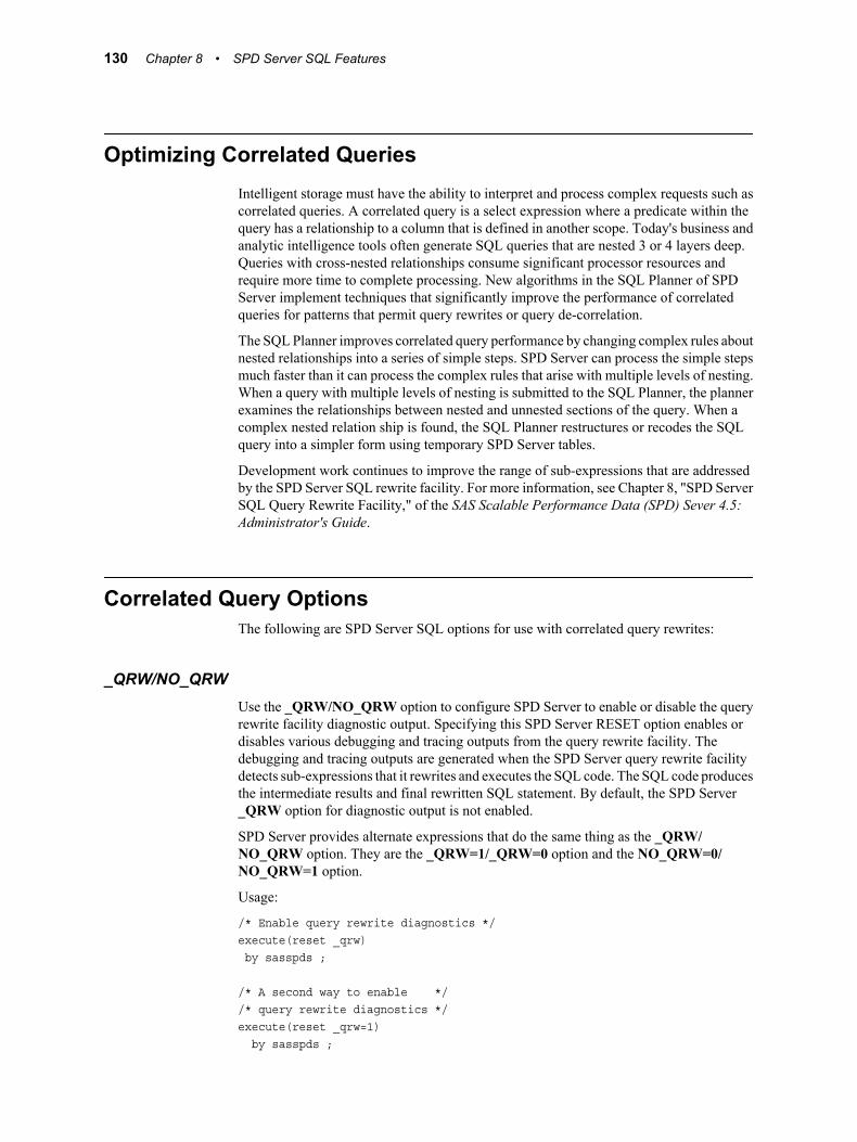
Optimizing Correlated QueriesIntelligent storage must have the ability to interpret and process complex requests such ascorrelated queries. A correlated query is a select expression where a predicate within thequery has a relationship to a column that is defined in another scope. Today's business andanalytic intelligence tools often generate SQL queries that are nested 3 or 4 layers deep.Queries with cross-nested relationships consume significant processor resources andrequire more time to complete processing. New algorithms in the SQL Planner of SPDServer implement techniques that significantly improve the performance of correlatedqueries for patterns that permit query rewrites or query de-correlation.

The SQL Planner improves correlated query performance by changing complex rules aboutnested relationships into a series of simple steps. SPD Server can process the simple stepsmuch faster than it can process the complex rules that arise with multiple levels of nesting.When a query with multiple levels of nesting is submitted to the SQL Planner, the plannerexamines the relationships between nested and unnested sections of the query. When acomplex nested relation ship is found, the SQL Planner restructures or recodes the SQLquery into a simpler form using temporary SPD Server tables.

Development work continues to improve the range of sub-expressions that are addressedby the SPD Server SQL rewrite facility. For more information, see Chapter 8, "SPD ServerSQL Query Rewrite Facility," of the SAS Scalable Performance Data (SPD) Sever 4.5:Administrator's Guide.

Correlated Query OptionsThe following are SPD Server SQL options for use with correlated query rewrites:

_QRW/NO_QRWUse the _QRW/NO_QRW option to configure SPD Server to enable or disable the queryrewrite facility diagnostic output. Specifying this SPD Server RESET option enables ordisables various debugging and tracing outputs from the query rewrite facility. Thedebugging and tracing outputs are generated when the SPD Server query rewrite facilitydetects sub-expressions that it rewrites and executes the SQL code. The SQL code producesthe intermediate results and final rewritten SQL statement. By default, the SPD Server_QRW option for diagnostic output is not enabled.

SPD Server provides alternate expressions that do the same thing as the _QRW/NO_QRW option. They are the _QRW=1/_QRW=0 option and the NO_QRW=0/NO_QRW=1 option.

Usage:

/* Enable query rewrite diagnostics */execute(reset _qrw) by sasspds ;

/* A second way to enable *//* query rewrite diagnostics */execute(reset _qrw=1) by sasspds ;


/* A third way to enable *//* query rewrite diagnostics */execute(reset no_qrw=0) by sasspds ;

/* Disable query rewrite diagnostics */execute(reset no_qrw) by sasspds ;

/* A second way to disable query *//* rewrite diagnostics */execute(reset _qrw=0) by sasspds ;

/* Another way to disable query *//* rewrite diagnostics */execute(reset no_qrw=1) by sasspds ;

_QRWENABLE/NO_QRWENABLEUse the _QRWENABLE/NO_QRWENABLE option to completely disable the SPDServer query rewrite facility. Disabling the query rewrite facility prevents the rewriteplanner from intervening in the SQL flow and from making any optimizing rewrites. Thisoption is not normally specified unless you want to test if an SQL statement would runfaster without rewrite optimization, or if you suspect that the resulting row set that you getfrom a query rewrite evaluation is incorrect.

SPD Server provides an alternate expression that does the same thing as the_QRWENABLE/NO_QRWENABLE option. It is the _QRWENABLE=1/_QRWENABLE=0 option. The query rewrite facility is enabled in SPD Server by default.

Usage:

/* Disable query rewrite *//* facility */execute(reset no_qrwenable) by sasspds ;

/* A second way to disable *//* query rewrite facility */execute(reset _qrwenable=0) by sasspds ;

/* Enable query rewrite *//* facility */execute(reset _qrwenable) by sasspds ;

/* A second way to enable *//* query rewrite facility */execute(reset _qrwenable=1) by sasspds ;

_QRWENABLE/NO_QRWENABLE 131

Materialized ViewsSPD Server allows users to create an SQL view as a materialized view. What makes amaterialized view different from an SQL view? For a materialized view, the results of theview statement are computed and saved in a temporary SPD Server table at the time theview is created. For a standard SQL view the results are computed each time the view isreferenced in a subsequent SQL statement. As long as there are no changes to any of theinput tables that the view consists of, the materialized view will return the results from thetemporary table when the view is referenced in an SQL statement. If any of the input tablesthat comprise the view are modified, the materialized view will recompute the results thenext time that the view is referenced and it will refresh the temporary table with the newresults. The materialized view temporary results table exists for as long as the view is inexistence. When a view is dropped or deleted, then the temporary results table is alsodeleted.

Materialized Views Operating DetailsA materialized view can be created only at the time the SQL view is created. This featureis available only through the SPD Server 4.5 SQL Pass-Through Facility. A new keywordMaterialized is added to the Create View syntax that identifies the view to be created as amaterialized view. When a materialized view is created, the Create View operation willnot complete until the temporary results table has been populated. This can add substantialtime to the execution of Create View.

Each time a created materialized view is referenced in an SQL statement, there is a checkto determine whether any of the input tables used to produce the temporary results tablehave been modified. If not, the temporary table is substituted in place of the vie w filewithin the SQL statement. If any of the input tables have been modified, the SQL statementwill execute without this substitution so it will act as if it is a standard SQL view reference.There is also a background thread launched at this time that is independent of the SQLstatement execution which will refresh the temporary results table. Until this refresh iscompleted, any incoming references to the view will be treated as standard view references.

Creating a standard SQL view results in a view file being created in the specified domainwith the name <viewname>.view.0.0.0.spds9. Creating a materialized view results in anadditional SPD Server table being created in the same domain as the view file with thename format <.viewname>.mdfspds9 and corresponding .dpf files <.viewname>.dpfspds9.The materialized view table is not visible or accessible to the user by using PROCDATASETS or other SAS procedures. If one or more simple indexes are defined on anyof the input tables that are used to create the results table, the indexes will also be createdon the materialized view table, as long as the column that was indexed in the input tablealso exists in the materialized view table.

User Interface for Materialized ViewsTo create a materialized view, use the following SQL Pass-Through syntax.

EXECUTE (Create Materialized View <viewname> as Select ) BY [sasspds | alias];

All other references to the view follow the existing SQL syntax, whether it is a standardSQL view or a materialized view. The Materialized keyword is used only in the Createstatement. For example, to drop a materialized view, you would use the following syntax.

EXECUTE (Drop View <viewname> ) BY [sasspds | alias];


If any of the input tables to a materialized view are modified, the next time the view isreferenced, a refresh is performed on the materialized view table. You can use anspdsserv.parm file option setting to specify the time delay before the materialized viewtable is refreshed.

MVREFRESHTIME=<number-of-seconds> ;

Where <number-of-seconds> specifies the number of seconds before the refresh will start.You can set the MVREFRESHTIME= option to any integer value between 0 and 86400.The default MVREFRESHTIME= specification is 30 seconds.

The reason that a time delay might be necessary before refreshing a materialized view tableis to prevent processor thrashing. Processor thrashing might occur if you refresh thematerialized view table when other processes are concurrently processing updates to thetables that are used in the view. If your computing environment does not perform multipleconcurrent table updates, then you can set MVREFRESHTIME=0 and eliminate any timedelay associated with materialized view refreshes.

Benefits of Materialized ViewsCreating a materialized view instead of a Standard SQL view can provide enormousperformance benefits when the view is referenced in an SQL statement. For views thatcontain costly operations such as multiple table joins or operations on very large tables,the execution time for queries containing a materialized view can be orders of magnitudeless than a standard view. If the results table produced by the view is relatively small incomparison with the input tables, the execution time for queries using a materialized viewmight be a few seconds versus several minutes for a standard view.

For example, if it takes on average 20 minutes to produce the result set from a view andthe result is in the order of thousands of rows or less, a query referencing the materializedview will now take seconds. Previously using the standard view operation s, every timethe view was referenced would result in 20 minutes of execution time. The performancebenefits should be measured on a case by case basis.

The decision of whether to use a standard view or a materialized view can be primarilydriven by how often the input tables to the view are updated versus how often the view isreferenced in an SQL statement. If a view is being referenced at least twice be fore anyupdates can occur, then the materialized view should provide superior performance. Incases where the defined view can be created very quickly, there is probably not a need forusing a materialized view. If the input tables are frequently updated in comparison to howoften the view is referenced, a standard view would probably be more efficient.

Materialized View ExampleThe following code shows the creation and use of a materialized view. The input tables Xand Z are created with X having three columns a,b,c and Z having four columns a,b,c,drespectively.

data mydomain.X; do a = 1 to 1000; b = sin(a); c = cos(a); output;end;run;

data mydomain.Z; do a = 500 to 1500;

Materialized View Example 133

b = sin(a); c = cos(a); d = mod(a,99); output;end;run;

PROC SQL;connect to sasspds (dbq='mydomain' host='myhost' serv='myport' user='me' passwd='mypasswd');

execute (create materialized view XZVIEW as select * from Z where a in (select a from X)) by sasspds;

select * from connection to sasspds (select * from XZVIEW where d >90);

execute (drop view XZVIEW);quit;

SPD Server SQL ExtensionsSPD Server SQL furnishes several extensions to the SQL language. These extensions arenot a part of standardized industry SQL, but they are an integral part of the SPD Serversystem. These extensions enable systemic data management unique to the SPD Server. TheSPD Server SQL uses a special Pass-Through Facility that uses these extensions for datamanipulation and extraction operations. The following section discusses the roles of thefollowing extensions which enable SPD Server's SQL Pass-Through Facility. In additionto the extensions in this section, users should know “Libref Statements” on page 96 and“Libref Clauses” on page 96.

BEGIN and END ASYNC OPERATION Statements

Overview of BEGIN and END ASYNC Operation StatementsAsynchronous statements are a useful technique you can use to harness the multi-processorpower of SPD Server. Asynchronous statements enable execution of multiple, independentthreads at the same time. The BEGIN ASYNC OPERATION and END ASYNCOPERATION statements allow you to delimit one or more statements for asynchronous,parallel execution. Since the statements execute in parallel, they must not depend onanother, because there is no way to guarantee which statement will finish before another


statement executes. SPD Server software initiates thread execution according to the orderof the statements in the block.

Usage:

execute ([ BEGIN | END ] ASYNCH OPERATION);

Illegal ASYNC Block StatementsThe statements in this Illegal ASYNC Block example have illegal interdependencies andcannot be expected to work correctly:

/* Example of Illegal ASYNC Block Code */

PROC SQL; connect to sasspds (dbq="my-domain" server=host.port user='user-name' password='user-password' other connection options);

execute(begin async operation) by sasspds;

execute(create table T1 as select * from SRC1) by sasspds;

execute(create unique index I1 on T1(a,b)) by sasspds;

execute(end async operation) by sasspds;


The example violates the interdependency rule. The create index statement assumes tableT1 exists and is complete. However, table T1 is created from table SRC1, and might notbe complete before the asynchronous create index statement executes. Hence, index I1 isdependent on a complete table T1. The resultant data would not be reliable. The purposeof this example is to illustrate the concept of interdependency, and how not to write anASYNC block.

Legal ASYNC Block StatementsThe statements in this Legal ASYNC Block example have no interdependencies.

/* Example of Legal ASYNC Block Code */ /* Creates some tables in the first ASYNC block */ /* */

PROC SQL; connect to sasspds

BEGIN and END ASYNC OPERATION Statements 135

(dbq="path1" server=host.port user='anonymous');


execute(create table state_al as select * from allstates where state='AL') by sasspds;

execute(create table state_az as select * from allstates where state='AZ') by sasspds; ...

execute(create table state_wy as select * from allstates where state='WY') by sasspds;


/* */ /* Create some indexes in the second ASYNC block */ /* */


execute(create index county on state_al(county)) by sasspds;

execute(create index county on state_az(county)) by sasspds; ...

execute(create index county on state_wy(county)) by sasspds;




Why does the second example work correctly? First, each table is created independently.Second, there is a 'synchronization point': the first END ASYNC operation. This pointensures that all the tables are created before the second ASYNC statement block begins.(You can also achieve results that are similar to this example by using the LOAD statement).

Using Librefs in an ASYNC Block StatementTo refer to a two-part table name inside an ASYNC block, you must re-execute the librefstatement issued before entering the block. Conversely, if you issue a libref statement insidethe ASYNC block, it does not extend outside the ASYNC block. An ASYNC block createsa distinct scope for the libref. To work correctly, a libref statement must be located insidethe ASYNC block, and the libref statement must precede the first SQL statement thatreferences it.

/* Example of Legal Code using LIBREFs in an ASYNC Block */ /* Create some tables in the first ASYNC block */

PROC SQL; connect to sasspds (dbq="path1" server=host.port user='anonymous');


execute(libref path1 engopt='dbq="path1" server=host.port user="anonymous"') by sasspds;


execute(create table path1.southeast as select a.customer_id, a.region, b.sales from path1.customer a, path2.orders b where a.customer_id = b.customer_id and a.region='SE') by sasspds;

....

execute(create table path1.northeast as select a.customer_id, a.region, b.sales from path1.customer a, path2.orders b where a.customer_id = b.customer_id and a.region='NE')

BEGIN and END ASYNC OPERATION Statements 137

by sasspds;



Using SQL Options in an ASYNC Block StatementSPD Server SQL options must be set globally for all execute statements in the ASYNCblock. These options must be set using an execute statement before the BEGIN ASYNCoperation. This example uses code blocks from the preceding example to show how to printa method tree without executing the SQL.

/* */ /* Example of Legal SQL Options in ASYNC Block */ /* */

PROC SQL; connect to sasspds (dbq="path1" server=host.port user='anonymous');

execute(reset noexec _method) by sasspds;




execute(create table path1.southeast as select a.customer_id, a.region, b.sales from path1.customer a, path2.orders b where a.customer_id = b.customer_id and a.region='SE') by sasspds;

....

execute(create table path1.northeast as


select a.customer_id, a.region, b.sales from path1.customer a, path2.orders b where a.customer_id = b.customer_id and a.region='NE') by sasspds;



LOAD StatementThe LOAD statement enables table creation (with one or more indexes) with a singlestatement. The data source for the statement is a SELECT clause. The SELECT list in theclause defines the columns for the new table. All characteristics of the columns (variables)in the select list are preserved, becoming permanent attributes of the new table's columndefinitions. The target table for the LOAD TABLE statement must be on the local machine.

Usage:

execute (LOAD TABLE table spec < WITH index spec < WITH index spec>> by sasspds;

In the following example, each execute statement creates a table for one U.S. state using aglobal table called STATE that contains many states. The first execute statement usesLOAD to create table STATE_AL (Alabama), and creates an index on the COUNTYcolumn. The structure of the state table STATE_AL and the data in the state table bothcome from the global table STATE. The data in STATE_AL is the subset of all recordsfrom STATE where the STATE column variable equals 'AL'. LOAD creates a table forstates from Alabama to Wyoming, with each state's table indexed by county and mirroringthe structure of the parent table STATE.

execute(load table state_al with index county on (county) as select * from state where state='AL') by sasspds;

execute(load table state_az with index county on (county) as select * from state where state='AZ') by sasspds;

LOAD Statement 139

...

execute(load table state_wy with index county on (county) as select * from state where state='WY') by sasspds;

In general, the LOAD statement is faster than a corresponding create table / create indexstatement pair, because it builds the table and associated index(es) asynchronously usingparallel processing.

COPY StatementThe COPY table statement creates a copy of an SPD Server table with or without the tableindex(es). For the COPY table statement to work, the source and target tables must be onthe local machine. By default, the software creates an index(es). The COPY table statementis faster than either of the following CREATE and LOAD statements:

create table ...as select ...create index ...

or

load table ...with index...as select ...

The COPY statement is faster than the two above statements because it uses a more directaccess path than the SQL SELECT clause when accessing the data.

In the example that follows, two new tables are created: T_NEWand T2_NEW. The firsttable, T_NEW, is created with index structures identical to table T_NEW. The second table,T2_NEW, is unindexed regardless of the structure of table T2_OLD.

execute(copy table t_new from t_old) by sasspds;

execute(copy table t2_new from t2_old without indexes) by sasspds;

The COPY statement also supports an ORDER BY clause you use to create a new tablewith a sort order on one or more columns of the new table. While COPY TABLE does notsupport all of the options of PROC SORT, you can achieve substantial performance gainswhen creating this ordered table by using COPY with an ORDER BY clause whenappropriate.

The next example copies the table T_OLD to T_NEW using the order by clause. The datawill be ordered by columns: x in ascending order, y in descending order, and z in ascendingorder. The results are the same if you run PROC SORT on the columns using the same BYclause. The syntax of the COPY ORDER BY follows the normal SQL ORDER BY clause,


but the column identifiers that you can specify are restricted. You can specify only actualtable columns when using the COPY ORDER BY clause.

execute(copy table t_new from t_old order by x, y desc, z asc) by sasspds;

Differences between SAS SQL and SPD ServerSQL

This section overviews some of the functional differences between SAS SQL and SPDServer SQL. A great deal of SAS SQL functionality is integrated into SPD Server.Exceptions between SAS and SPD Server SQL are listed below.

Reserved KeywordsSPD Server uses keywords to initiate statements or refer to syntax elements. For example,the words where and group can be used only in certain ways, because there are WHEREand GROUP BY clauses. Keywords are treated as reserved words. That means you cannotuse keywords when naming a libref, a table, a column or an index.

In contrast, SAS allows keywords in some, but not all, syntax locations. The documentationchapter “SPD Server SQL Syntax Reference Guide” on page 145 contains a list of“(Reserved) Keywords” on page 148.

Table Options and DelimitersSPD Server SQL uses brackets to delimit table options. SAS SQL uses parentheses asdelimiters. You can place table options in a create table statement. You must put tableoptions within parentheses to delimit column definitions within a table.

Mixing Scalar Expressions and Boolean PredicatesSPD Server SQL does not allow mixing scalar expressions with Boolean predicates. SASSQL does allow mixing scalar expressions with Boolean predicates in most places. TheHelp section on “Scalar Expressions Contrasted with Boolean Predicates” on page 147contains more information about permissible expression content.

INTO ClauseSPD Server SQL does not support the INTO clause, as in

select a, b into :var1, :var2 from t where a > 7;

In contrast, SAS SQL supports the INTO clause.

Tilde NegationSPD Server SQL supports the use of the tilde only to negate the 'equals' operator, ~= (notequals). SAS SQL allows broader use of the tilde ('~') character, where the tilde is

Tilde Negation 141

synonymous with not and can be combined with various operators. For example, SAS SQLcan use the tilde with 'between' ~ between (not between). SPD Server does not recognizethat expression.

Nested QueriesSAS SQL permits sub-queries without parentheses delimiters in more places than SPDServer SQL. SPD Server SQL uses parentheses to explicitly group sub-queries orexpressions that are nested within a query statement whenever possible. Queries withnested expressions execute more reliably and are also easier to read.

USER ValueSAS SQL permits sub-queries without parentheses delimiters in more places than SPDServer SQL. SPD Server SQL uses parentheses whenever possible to explicitly group sub-queries or expressions that are nested within a query statement. Queries with nestedexpressions execute more reliably and are easier to read.

SPD Server SQL does not support the USER keyword in the INSERT statement. Forexample, the following query will fail in SPD Server SQL:

insert into t1(myname) values(USER);

Supported FunctionsSPD Server SQL supports the following functions:

abs, addr, arcos, arsin, atan, band, betainv, blshift, bnot, bor, brshift, bxor,byte, ceil, cinv, collate, compbl, compound, compress, cos, cosh, css, cv,daccdb, daccdbsl, daccsl, daccsyd, dacctab, date, datejul, datepart, datetime,day, dcss, depdb, depdbsl, depsl, depsyd, deptab, dequote, dhms, digamma, dmax,dmean, dmin, drange, dstd, dstderr, dsum, duss, dvar, erf, erfc, exp, finv,fipname, fipnamel, fipstate, floor, fnonmiss, fuzz, gaminv, gamma, hms, hour,int, intck, intnx, intrr, irr, ispexec, isplink, kurtosis, left, length, lgamma,log, log10, log2, lowcase, max, mdy, mean, min, minute, mod, month, mort, n,netpv, nmiss, npv, ordinal, poisson, probbeta, probbnml, probchi, probf, probgam,probhypr, probit, probnegb, probnorm, probt, qtr, quote, range, ranuni, rank,recip, repeat, reverse, right, round, saving, second, sign, signum, sin, sinh,skewness, sqrt, std, stderr, stfips, stname, stnamel, substr, sum, tan, tanh,time, timepart, tinv, today, tranwrd, trigamma, trim, upcase, uss, var, weekday,year, zipfips, zipname, zipnamel, and zipstate.

Ranuni functions can show slight variation from run to run due to the impact of parallelprocessing.

Note that date, int, left, right and trim are reserved keywords. Therefore, they must bepreceded by a backslash in SPD Server SQL queries:

select \date() from t ;


Part 4

SPD Server SQL Reference

Chapter 9SPD Server SQL Syntax Reference Guide . . . . . . . . . . . . . . . . . . . . . . . 145

Chapter 10SAS Scalable Performance Data (SPD) Server SQL Access Library APIReference . . . . . . . . . . . . . . . . . . . . . . . . . . . . . . . . . . . . . . . . . . . . . . . . . . . . . . 159

143

Chapter 9SPD Server SQL SyntaxReference Guide

Overview . . . . . . . . . . . . . . . . . . . . . . . . . . . . . . . . . . . . . . . . . . . . . . . . . . . . . . . . . . . 146

Document Conventions . . . . . . . . . . . . . . . . . . . . . . . . . . . . . . . . . . . . . . . . . . . . . . . 146Productions . . . . . . . . . . . . . . . . . . . . . . . . . . . . . . . . . . . . . . . . . . . . . . . . . . . . . . . 146Production Links / References . . . . . . . . . . . . . . . . . . . . . . . . . . . . . . . . . . . . . . . . 146Literal Text . . . . . . . . . . . . . . . . . . . . . . . . . . . . . . . . . . . . . . . . . . . . . . . . . . . . . . 146Optional Text . . . . . . . . . . . . . . . . . . . . . . . . . . . . . . . . . . . . . . . . . . . . . . . . . . . . . 146Selection Lists . . . . . . . . . . . . . . . . . . . . . . . . . . . . . . . . . . . . . . . . . . . . . . . . . . . . 146

SQL Syntax Definitions . . . . . . . . . . . . . . . . . . . . . . . . . . . . . . . . . . . . . . . . . . . . . . . 147Statement (Query) . . . . . . . . . . . . . . . . . . . . . . . . . . . . . . . . . . . . . . . . . . . . . . . . . . 147Scalar Expressions Contrasted with Boolean Predicates . . . . . . . . . . . . . . . . . . . . 147Strings . . . . . . . . . . . . . . . . . . . . . . . . . . . . . . . . . . . . . . . . . . . . . . . . . . . . . . . . . . . 147Identifiers . . . . . . . . . . . . . . . . . . . . . . . . . . . . . . . . . . . . . . . . . . . . . . . . . . . . . . . . 148(Reserved) Keywords . . . . . . . . . . . . . . . . . . . . . . . . . . . . . . . . . . . . . . . . . . . . . . . 148

SQL Statements . . . . . . . . . . . . . . . . . . . . . . . . . . . . . . . . . . . . . . . . . . . . . . . . . . . . . 148Alter Table Statement . . . . . . . . . . . . . . . . . . . . . . . . . . . . . . . . . . . . . . . . . . . . . . . 148Connect Statement . . . . . . . . . . . . . . . . . . . . . . . . . . . . . . . . . . . . . . . . . . . . . . . . . 148Create Index Statement . . . . . . . . . . . . . . . . . . . . . . . . . . . . . . . . . . . . . . . . . . . . . . 149Create Table Statement . . . . . . . . . . . . . . . . . . . . . . . . . . . . . . . . . . . . . . . . . . . . . . 149Create View Statement . . . . . . . . . . . . . . . . . . . . . . . . . . . . . . . . . . . . . . . . . . . . . . 149Delete Statement . . . . . . . . . . . . . . . . . . . . . . . . . . . . . . . . . . . . . . . . . . . . . . . . . . . 149Describe Table Statement . . . . . . . . . . . . . . . . . . . . . . . . . . . . . . . . . . . . . . . . . . . . 149Describe View Statement . . . . . . . . . . . . . . . . . . . . . . . . . . . . . . . . . . . . . . . . . . . . 149Disconnect Statement . . . . . . . . . . . . . . . . . . . . . . . . . . . . . . . . . . . . . . . . . . . . . . . 150Drop Index Statement . . . . . . . . . . . . . . . . . . . . . . . . . . . . . . . . . . . . . . . . . . . . . . . 150Drop Table Statement . . . . . . . . . . . . . . . . . . . . . . . . . . . . . . . . . . . . . . . . . . . . . . . 150Drop View Statement . . . . . . . . . . . . . . . . . . . . . . . . . . . . . . . . . . . . . . . . . . . . . . . 150Execute Statement . . . . . . . . . . . . . . . . . . . . . . . . . . . . . . . . . . . . . . . . . . . . . . . . . 150Insert Statement . . . . . . . . . . . . . . . . . . . . . . . . . . . . . . . . . . . . . . . . . . . . . . . . . . . 150Reset Statement . . . . . . . . . . . . . . . . . . . . . . . . . . . . . . . . . . . . . . . . . . . . . . . . . . . 151Select Statement . . . . . . . . . . . . . . . . . . . . . . . . . . . . . . . . . . . . . . . . . . . . . . . . . . . 151Update Statement . . . . . . . . . . . . . . . . . . . . . . . . . . . . . . . . . . . . . . . . . . . . . . . . . . 151Validate Statement . . . . . . . . . . . . . . . . . . . . . . . . . . . . . . . . . . . . . . . . . . . . . . . . . 151

NEW SQL Statements . . . . . . . . . . . . . . . . . . . . . . . . . . . . . . . . . . . . . . . . . . . . . . . . 151Async Operation Statement . . . . . . . . . . . . . . . . . . . . . . . . . . . . . . . . . . . . . . . . . . 151Copy Table Statement . . . . . . . . . . . . . . . . . . . . . . . . . . . . . . . . . . . . . . . . . . . . . . . 151Create Materialized View Statement . . . . . . . . . . . . . . . . . . . . . . . . . . . . . . . . . . . 152Libref Statement . . . . . . . . . . . . . . . . . . . . . . . . . . . . . . . . . . . . . . . . . . . . . . . . . . . 152Load Table Statement . . . . . . . . . . . . . . . . . . . . . . . . . . . . . . . . . . . . . . . . . . . . . . . 152

SQL Building Blocks . . . . . . . . . . . . . . . . . . . . . . . . . . . . . . . . . . . . . . . . . . . . . . . . . 152

145

OverviewThis chapter describes the SQL syntax that is allowed with the Scalable Performance Data(SPD) Server. SPD Server SQL is a dialect of SQL. That is, it combines SQL-92, SASSQL and extensions that are specific to SPD Server. Whenever possible, SPD Serverattempts to conform to SAS SQL.

Document Conventions

ProductionsThe syntax uses building blocks which are referred to as productions. Productions aredenoted by the symbol ::= . To the left of the equal sign is a production name; to the rightof the equal, or on the next line, is a list of production constructs. If a production has morethan one possible construct, the alternatives are separated by a vertical bar |. Readproductions top-down. For example, reading the delete statement, there are literal keywordsand two subproductions, a table_spec and the WHERE clause.

Production Links / ReferencesSubproductions that are referenced within a production definition are HTML links to theirdefinitions. You can navigate the links with an HTML browser.

Literal TextTraversing down a syntax tree leads to leaf/terminal definitions. The definitions arecomposed either of keywords (select), identifiers (names of tables, columns, and so on) orsymbols ( punctuation, operators, and so on.). Keywords and identifiers are shown withbold, capitalized text. In contrast, symbols are shown with single quotation marks and arebold.

Optional TextOptional syntax is delimited by square brackets, [ and ]. Optional lists (syntax elementsthat are repeated) are denoted by [ and ]*. The * signifies zero or more occurrences of thebracketed syntax.

Selection ListsSelection lists, that allow you to choose from a list of alternative syntax elements, aredenoted by braces { and }. These elements are separated by a vertical bar |. The selectionlist itself is not optional; you must choose at least one element. If you must choose one ormore of the elements, the list is terminated with a }+. The + indicates one or moreoccurrences of the delimited syntax.

Note: The browser displays links best with underscores. To view underscores usingNetscape, refer to the option under the File Command: Options/General Preferences/Appearance.

146 Chapter 9 • SPD Server SQL Syntax Reference Guide

SQL Syntax Definitions

Statement (Query)One or more syntax elements terminated by a semicolon.

Scalar Expressions Contrasted with Boolean PredicatesScalar expressions represent a single data value, either a numeric or a string from a constantspecification. Examples include: 1, 'hello there', '31-DEC-60'd), a function (that is,avg(a*b)), a column/variable (that is foo.bar), the case expression, or even a subquerywhich returns a single run-time value. Boolean predicates are either true or false. They areused in WHERE clauses, having clauses and in the case expression. You cannot selectpredicates, nor can you assign them to columns (that is, in an update statement). Scalarexpressions and Boolean predicates cannot be used interchangeably, although SAS SQLdoes allow you to mix the expressions.

StringsSPD Server SQL strings are character streams which are delimited by either single or doublequotation marks. If you use a single quotation mark to begin a string, you must use a singlequotation mark to terminate the string. To embed a single quotation mark in a string, usetwo single quotation marks together. For example,

SELECT 'it''s a wonderful life' from mytable.

You can use double quotation marks in the same manner. There is another way to embeda single quotation mark without doubling the character. You can use double-quotationmarks as delimiters. For example,

SELECT it's a wonderful life from mytable.

In some of the syntax specifications that follow, a user-defined or database-specific stringis noted. Delimit these strings with a bracket or parenthesis. Characters between thedelimiters are considered part of the string up to, but not including, the matching delimiter.

CONNECT to sasspds( user='john' passwd='foobar' options=(a b c) );

The dbms_options string is

user='john' passwd='foobar' options=(a b c).

In this example, the first right-parenthesis is considered part of the string. It is not thematching termination delimiter.

Strings 147

IdentifiersIdentifiers are the names of librefs, tables, indexes and columns as well as table and columnaliases.

(Reserved) KeywordsKeywords are used to initiate statements and syntax elements. For example, WHERE orGROUP BY clauses. Keywords are also reserved. They cannot be used for identifiersbecause this use introduces ambiguity. For example, select unique from; is a valid butambiguous statement. Below is a list of current SPD Server keywords. Some words havebeen reserved for future enhancements to SPD Server SQL:

add, all, alter, and, any, as, asc, async, begin, between, both, by,calculated, cascade, case, char, character, column, connect,connection, contains, contents, copy, corr, corresponding, create,cross, date, dec, decimal, default, delete, desc, describe,dictionary, disconnect, distinct, double, drop, else, end, engname,engopt, eq, except, execute, exists, false, float, for, format, from,full, ge, grant, group, gt, having, in, index, indexes, informat,inner, insert, int, integer, intersect, into, is, join, label, le,leading, left, libref, like, load, lower, lt, match, missing, modify,natural, ne, no, not, notin, null, num, numeric, on, operation, option,or, order, outer, overlaps, partial, precision, privileges, public,real, references, reset, restrict, revoke, right, select, set,smallint, some, table, then, to, trailing, trim, true, union, unique,unknown, update, upper, using, validate, values, varchar, verbose,view, when, where, with, without, yes

SQL Statements

Alter Table StatementThe Alter table statement changes a table definition.

alter table statement ::= ALTER TABLE table spec { { ADD|MODIFY|ALTER [ COLUMN ] column def list } | { DROP [ COLUMN ] column name list } }+ ';'

Connect StatementThe Connect statement creates a pass-through connection.

connect statement ::= CONNECT TO libref name [ [ AS ] alias name ] '(' dbms options ')' ] ';'


Create Index StatementThe Create Index statement creates an index on a table.

create index statement ::= CREATE [ UNIQUE ] INDEX index name ON table spec '(' column name list ')' ';'

Create Table StatementThe Create Table statement creates a table definition.

create table statement ::= CREATE TABLE table spec { '(' column def list ')' | ASselect spec | LIKEtable spec } ';'

Create View StatementThe Create View statement creates a view upon one or more tables.

create view statement ::= CREATE VIEWtable spec ASselect spec ';'

Delete StatementThe Delete statement deletes records.

delete statement ::= DELETE FROMtable spec [where clause ] ';'

Describe Table StatementThe Describe Table statement describes a table definition.

describe table statement ::= DESCRIBE TABLE table spec [ [','] table spec ]* ';'

Describe View StatementThe Describe View statement describes a view definition.

describe view statement ::= DESCRIBE VIEW table spec [ [','] table spec ]* ';'

Describe View Statement 149

Disconnect StatementThe Disconnect statement is a pass-through statement.

disconnect statement ::= DISCONNECT FROMlibref name ';'

Drop Index StatementThe Drop Index statement drops an index from a table.

drop index statement ::= DROP INDEX index name [ [','] index name ]* FROM table spec ';'

Drop Table StatementThe Drop Table statement drops a table definition.

drop table statement ::= DROP TABLEtable spec [ [',']table spec ]* ';'

Drop View StatementThe Drop View statement drops a view definition.

drop view statement ::= DROP VIEW table spec [ [','] table spec ]* ';'

Execute StatementThe Execute statement is a pass-through statement.

execute statement ::= EXECUTE '('passthru spec ')' BYlibref name ';'

Insert StatementThe Insert statement adds records.

insert statement ::= INSERT INTO table spec [ '(' column name list ')' ] insert source ';'


Reset StatementThe Reset statement resets session options and flags.

set option statement ::= { SET OPTION | RESET } { identifier [ '=' { constant |identifier |truth value| DEFAULT } ] }+

Select StatementThe Select statement retrieves information.

select statement::=select spec ';'

Update StatementThe Update statement updates records.

update statement ::= UPDATE table spec SET column name '='scalar expr [ ','column name '='scalar expr ]* [ where clause ] ';'

Validate StatementThe Validate statement validates a given select specification.

validate statement ::= VALIDATEselect spec ';'

NEW SQL Statements

Async Operation Statementasync operation statements ::= { BEGIN | END } ASYNC OPERATION ';'

Copy Table Statementcopy table statement ::= COPY TABLE table spec FROM

Copy Table Statement 151

table spec [ WITHOUT INDEXES ] [ORDER BY column name [ ASC | DESC ] [',' column name [ ASC | DESC ]]] ';'

Create Materialized View Statementcreate materialized view statement ::= CREATE MATERIALIZED VIEWtable spec ASselect spec ';'

Libref Statementlibref statement ::= LIBREF libref name [ ENGNAME '=' identifier ] [ ENGOPT '=' string ] ';'

Load Table Statementload table statement ::= LOAD TABLE table spec [ WITH with index spec [ ',' with index spec ]* ] AS select spec ';'

SQL Building BlocksAlias Name

alias name ::=identifier

Atomic Expression

atomic expr ::=constant |column spec

Between Predicate

between pred ::=scalar expr [ NOT ] BETWEENscalar expr ANDscalar expr

Boolean Expression

boolean expr ::= | [ NOT ] { predicate | '(' boolean expr ')' } [ IS [ NOT ] truth value ]


| boolean expr { AND | OR } boolean expr

Case Expression

case expr ::= CASE { WHEN boolean expr THEN scalar expr }+ [ ELSE scalar expr ] END | CASE scalar expr { WHEN scalar expr THEN scalar expr }+ [ ELSE scalar expr ] END

Column Definition

column def ::=column namedata type [column modifier ]* [ NOT NULL ]

Column Definition List

column def list ::=column def [ ','column def ]*

Column Modifier

column modifier ::= FORMAT '=' <quoted or nonquoted SAS format specification> | LABEL '=' string

Column Name

column name ::= identifier

Column Name List

column name list ::=column name [ [',']column name ]*

Column Specifications

column spec ::= [ CALCULATED ] column name | table alias'.' column name

Comparative Operators

comp operator ::= | EQ | '=' | NE | '^=' | '~=' | '!=' | '<>' | LT | '<' | GT | '>' | LE | '<=' | GE | '>='

Comparison Predicates

comparison pred ::=scalar expr {

SQL Building Blocks 153

comp operatorscalar expr }+

Connection String

connection string ::= <user-definedstring delimited by ending/matching parenthesis>

Constant

constant ::= | number | missing value | string | date/time string | NULL

Contains Predicate

contains pred ::=scalar expr { CONTAINS | '?' }scalar expr

Data Types

data type ::= { CHAR[ACTER] | VARCHAR } [ '('unsigned ')' ] | { INT[EGER] | SMALLINT } | { NUM[ERIC] | DEC[IMAL] | FLOAT } [ '(' unsigned [ ',' unsigned ] ')' ] | REAL | DOUBLE PRECISION | DATE

Date / Time String

date/time string ::=string{D|T|DT}

DBMS Options

dbms options ::= <user-definedstring delimited by ending/matching parenthesis>

Digits (Numeric)

digit ::= '0' <through> '9'

Exists Predicate

exists pred ::= EXISTS subquery

Function Arguments

function args ::= scalar expr [ ',' scalar expr ]* | DISTINCT scalar expr | [ DISTINCT ] '*'

Function Expressions

function expr ::=func name '('function args ')'

Function Name

function name ::=identifier

Identifier

identifier ::= ['\']{letter|<underscore>}{


letter|digit|<underscore>}*

In Predicate

in pred ::= scalar expr { [ NOT ] IN | NOTIN } { subquery | '(' constant [ ',' constant ]* ')' }

Index Name

index name ::=identifier

Insert Set List

insert set list ::= SETset value list [ SETset value list ]*

Insert Source

insert source ::= | insert values list | insert set list | query expr

Insert Value

insert value ::= VALUES '('scalar expr [ ','scalar expr ]* ')'

Insert Values List

insert values list ::=insert value [insert value ]*

Letter (Alpha)

letter ::= 'a' <through> 'z' <or> 'A' <through> 'Z'

Libref Name

libref name ::=identifier

LIKE Predicate

like pred ::=scalar expr [ NOT ] LIKEscalar expr

Missing Value

missing value ::= '.'[letter]

Null Predicate

null pred ::=scalar expr IS [ NOT ] { NULL | MISSING }

Number


number ::= {unsigned|{ digit}+'.'[{ digit}+]|'.'{ digit}+}[{'e'|'E'}['+'|'-']{ digit}+]

ORDER BY Clause

order by clause ::= ORDER BY atomic expr [ ASC | DESC ] [ ',' atomic expr [ ASC | DESC ] ]*

Pass-Through Spec

passthru spec ::= <database-specific string delimited by ending/matching parenthesis>

Predicate Types

predicate ::= | comparison pred | between pred | in pred | like pred | null pred | quantified comparison pred | exists pred | contains pred | soundslike pred

Quantified Comparison Predicate

quantified comparison pred ::= scalar expr comp operator { ALL | SOME | ANY } subquery

Query Expression

query expr ::= query spec | query expr { [ OUTER ] UNION | EXCEPT | INTERSECT } [ CORRESPONDING ] [ ALL ] query expr

Query Spec

query spec ::= SELECT [ DISTINCT | UNIQUE ] select item [ ',' select item ]* FROM table ref [ ',' table ref ]* [ WHERE boolean expr ] [ GROUP BY scalar expr [ ',' scalar expr ]* ] [ HAVING boolean expr ]

Scalar Expression

scalar expr ::= | atomic expr | function expr


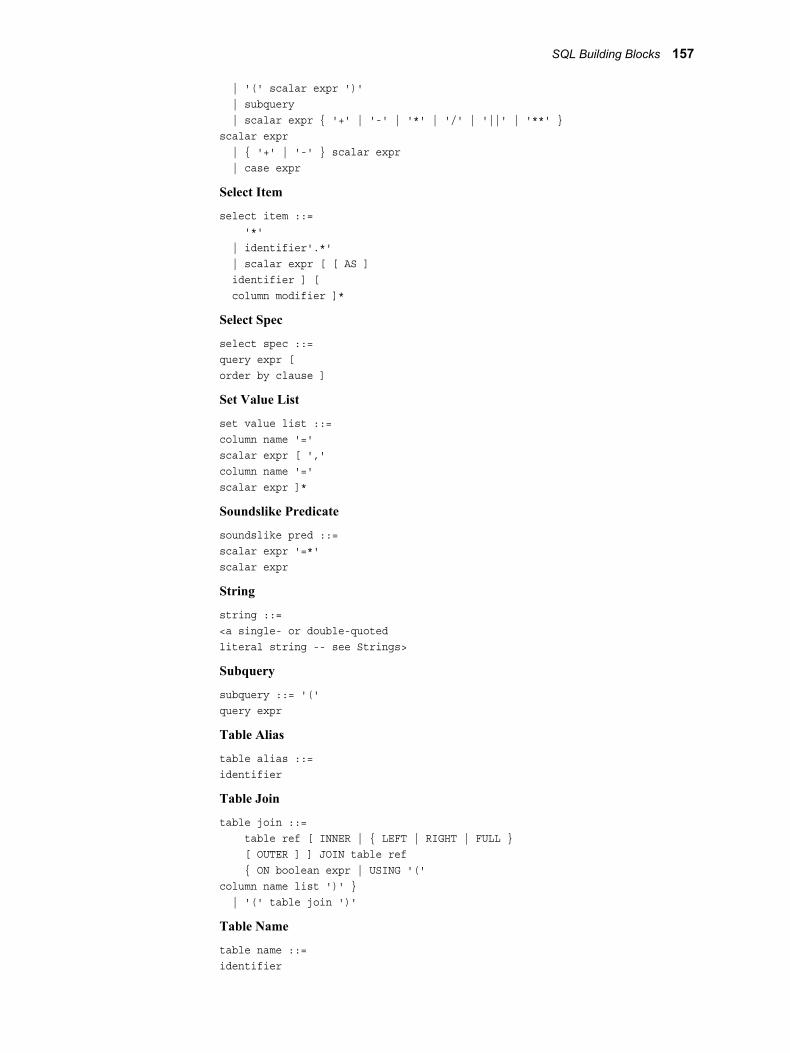
| '(' scalar expr ')' | subquery | scalar expr { '+' | '-' | '*' | '/' | '||' | '**' }scalar expr | { '+' | '-' } scalar expr | case expr

Select Item

select item ::= '*' | identifier'.*' | scalar expr [ [ AS ] identifier ] [ column modifier ]*

Select Spec

select spec ::=query expr [order by clause ]

Set Value List

set value list ::=column name '='scalar expr [ ','column name '='scalar expr ]*

Soundslike Predicate

soundslike pred ::=scalar expr '=*'scalar expr

String

string ::=<a single- or double-quotedliteral string -- see Strings>

Subquery

subquery ::= '('query expr

Table Alias

table alias ::=identifier

Table Join

table join ::= table ref [ INNER | { LEFT | RIGHT | FULL } [ OUTER ] ] JOIN table ref { ON boolean expr | USING '('column name list ')' } | '(' table join ')'

Table Name

table name ::=identifier


Table Options

table options ::= <user-defined string delimited by ending/matching bracket>

Table Reference

table ref ::= table spec [ [ AS ] identifier ] | subquery [ [ AS ] identifier ] [ '(' column name list ')' ] | CONNECTION TO identifier '(' connection string ')' [ [ AS ] identifier ] | table join

Table Spec

table spec ::= | table name [ '[' table options ']' ] | libref name'.' table name [ '[' table options ']' ]

Truth Value

truth value ::= { TRUE | YES } | { FALSE | NO }

Unsigned

unsigned ::= {digit }+

WHERE Clause

where clause ::= WHEREboolean expr

With Index Spec

with index spec ::= [ UNIQUE ] INDEXindex name ON '('column name list ')'


Chapter 10SAS Scalable Performance Data(SPD) Server SQL Access LibraryAPI Reference

Introduction . . . . . . . . . . . . . . . . . . . . . . . . . . . . . . . . . . . . . . . . . . . . . . . . . . . . . . . . . 159

Overview of SPQL Usage . . . . . . . . . . . . . . . . . . . . . . . . . . . . . . . . . . . . . . . . . . . . . . 160

SPQL API Description . . . . . . . . . . . . . . . . . . . . . . . . . . . . . . . . . . . . . . . . . . . . . . . . 160

SPQL API Functions . . . . . . . . . . . . . . . . . . . . . . . . . . . . . . . . . . . . . . . . . . . . . . . . . 160spqlinit() . . . . . . . . . . . . . . . . . . . . . . . . . . . . . . . . . . . . . . . . . . . . . . . . . . . . . . . . . 160spqlterm() . . . . . . . . . . . . . . . . . . . . . . . . . . . . . . . . . . . . . . . . . . . . . . . . . . . . . . . . 160spqlconnect() . . . . . . . . . . . . . . . . . . . . . . . . . . . . . . . . . . . . . . . . . . . . . . . . . . . . . . 161spqldisconnect() . . . . . . . . . . . . . . . . . . . . . . . . . . . . . . . . . . . . . . . . . . . . . . . . . . . 161spqlperform() . . . . . . . . . . . . . . . . . . . . . . . . . . . . . . . . . . . . . . . . . . . . . . . . . . . . . 161spqlfreestok() . . . . . . . . . . . . . . . . . . . . . . . . . . . . . . . . . . . . . . . . . . . . . . . . . . . . . 162spqltabinfo() . . . . . . . . . . . . . . . . . . . . . . . . . . . . . . . . . . . . . . . . . . . . . . . . . . . . . . 162spqlcolinfo() . . . . . . . . . . . . . . . . . . . . . . . . . . . . . . . . . . . . . . . . . . . . . . . . . . . . . . 163spqlfetch() . . . . . . . . . . . . . . . . . . . . . . . . . . . . . . . . . . . . . . . . . . . . . . . . . . . . . . . . 163spqlgmsg() . . . . . . . . . . . . . . . . . . . . . . . . . . . . . . . . . . . . . . . . . . . . . . . . . . . . . . . 163

SPQL Function Return Codes . . . . . . . . . . . . . . . . . . . . . . . . . . . . . . . . . . . . . . . . . . 164SPQL_SUCCESS(==0) . . . . . . . . . . . . . . . . . . . . . . . . . . . . . . . . . . . . . . . . . . . . . 164SPQL_ENDDATA(WARNING) . . . . . . . . . . . . . . . . . . . . . . . . . . . . . . . . . . . . . . 164SPQL_INITFAILED(ERROR) . . . . . . . . . . . . . . . . . . . . . . . . . . . . . . . . . . . . . . . 164SPQL_NOMEM . . . . . . . . . . . . . . . . . . . . . . . . . . . . . . . . . . . . . . . . . . . . . . . . . . . 164SPQL_CONFAILED(ERROR) . . . . . . . . . . . . . . . . . . . . . . . . . . . . . . . . . . . . . . . 164SPQL_BADSTMT(ERROR) . . . . . . . . . . . . . . . . . . . . . . . . . . . . . . . . . . . . . . . . . 164

IntroductionThis chapter describes the Scalable Performance Data Server SQL access library API(Application Programming Interface) and provides some simple examples. This chapterrefers to the Scalable Performance Data Server SQL access library as SPQL. Read thischapter if you want a library that provides a C-language compatible interface to write userapplications to access an SPD Server SQL server. Because the library was designed formulti-threaded applications, the code is thread safe.

159

Overview of SPQL UsageSPQL enables you to write application: programs that can connect to and access ScalablePerformance Data Server (SPD Server) hosts using the SQL language. SPQL is orientedtoward connection, allowing you to submit SQL statements to one or more SPD ServerSQL servers which execute SQL statements on your behalf.

SPQL API DescriptionThe C-language H file spql.h is provided for customer-written applications. This chapterdescribes the API functions, their use, and restrictions.

SPQL API FunctionsThe SPQL API functions include

spqlinit()Initializes the SPQL library for operation.

int spqlinit(void)

Usage: Performs a one-time initialization which enables the SPQL library to function. Forthis reason, you must call spqlinit() at least once to activate an SPQL program. Do not makeother SPQL API calls before calling this function. If you do, the results are unpredictable.When spqlinit() successfully completes, you can safely proceed to use the SPQL API in amulti-threaded context.

Note: Spqlinit()-is not a thread-safe function. Call it only within a single-threaded contextin your application. Alternatively, call it within an application-controlled mutex region.

Parameters: None

Returns: 0 if successful; SPQL_INITFAILED if the initialization fails.

spqlterm()Is the termination counterpart of the spqlinit() function.

int spqlterm(void)

Usage: Terminates the SPQL library session, disconnecting all active SPD Server SQLserver connections and freeing up the memory resources associated with the SPQL run-time library executables.

Parameters: None

Returns: 0 if successful.

160 Chapter 10 • SAS Scalable Performance Data (SPD) Server SQL Access Library API Reference

spqlconnect()Establishes a connection to a specified SPD Server SQL server.

int spqlconnect(char *constr, void **contok)

Usage: Establishes a connection to the SPD Server SQL server. The constr parameterspecifies all the connection information needed to establish the connection to an SPD ServerSQL server. When a connection is made successfully, a connection, token (contok) isreturned to the caller.

Parameters:

char *constrA null-terminated string identifying the SPD Server SQL server to connect to for thissession. The syntax for the string is identical to that used for the SAS PROC SQL pass-through CONNECT statement.

void **contokReturns a connection token if the connection successfully completes. You must retainthe token; use it in subsequent SPQL library operations that you perform using theconnection.

Returns: 0 if successful; SPQL_NOMEM if unable to allocate memory for the connectiontoken; SPQL_CONFAILED if unable to connect successfully to the SPD Server SQLserver.

spqldisconnect()Terminates a connection from the SPD Server SQL server specified with a spqlconnect().

int spqldisconnect(void *contok)

Usage: Disconnects from a specified SPD Server SQL server. The caller passes theconnection token which was returned from an spqlconnect() call. Then, the SPD ServerSQL server associated with the connection is disconnected from the caller, and the memoryassociated with connection token is returned to the system.

Parameters:

void *contokConnection token previously obtained from spqlconnect().


spqlperform()Submits an SQL statement for execution on a given connection.

int spqlperform(void *contok, char *stmtbuf, int stmtlen, int *actions, void **stmttok);

Usage: Performs specified SQL statement and informs caller of the results. The actionsparameter returns a value of 0 if no additional action is required. If actions are required tocomplete the statement, one or more of the following bit flags are returned.

Flag Action ---------- ---------------

spqlperform() 161

SPQLDATA Data is returned(see spqlfetch()) SPQLCOLINFO Column information is returned(see spqlcolinfo())

Parameters:

void *contokThe connection used to execute the SQL statement.

char *stmtbufA buffer that holds the SQL statement to perform.

int stmtlenThe length of the SQL statement in buffer; -1 if null-terminated.

int *actionsReturns post-processing notification bit flags.

void **stmttokReturns a statement token to use in post-processing the SQL statement results. See post-processing action definitions for use of statement token.

Returns: 0 if the SQL statement is successfully prepared/executed; SPQL_BADSTMT ifthe SQL statement specified in the statement buffer is prepared incorrectly;SPQL_NOMEM if spqlperform cannot allocate memory for the statement token.

spqlfreestok()

Generates a free statement token from spqlperform().

int spqlfreestok(void *stmttok);

Usage: Free resources used for the statement token from spqlperform(). Callspqlfreestok() after the data/information from the statement token has been extracted. Youcan call this function before all selected rows from the spqlperform() are read. If you do,the remaining unread rows (from the previous select) are discarded.

Parameters:

void *stmttokStatement token to free


spqltabinfo()

Gets table information from a statement token.

int spqltabinfo(void *stmttok, spqltinfo_t **tinfo)

Usage: Interrogates the statement token for table information. Upon return of the call,updates tinfo with the pointer to the spqltinfo_t structure in the statement.

Note: Treat the structure accessed by the returned pointer as read-only memory.

Parameters:

void *stmttokThe statement token to use to access table information from a 'select'.

spqltinfo **tinfoReturns pointer to spqltinfo_t structure into the statement token memory.

Returns: 0 for successful completion.


spqlcolinfo()Gets column information from a statement token.

int spqlcolinfo(void *stmttok, int *ncols, spqlcinfo_t **colvec)

Usage: Interrogates token for column information. Upon return of the call, updates ncolswith the column count selected in the statement and updates colvec with the pointer to thevector of spqlcol_t structures in the statement.

Note: Treat structures accessed by the returned pointer as read-only memory.

Parameters:

void *stmttokThe statement token to use to access column information from 'select'.

int *ncolsReturns in the statement token the number of columns selected.

spqlcinfo **colvecReturns in the statement token a pointer to the array of spqlcinfo_t structures.

Returns:0 if successful.

spqlfetch()

Gets row data from a statement token.

int spqlfetch(void *stmttok, void **bufptr, int *bufsize)

Usage: Fetches the rows returned from executing a statement. Each call to spqlfetch returnsa row from a statement to the caller's buffer. If bufptr contains a NULL value, the routinereturns a pointer to a buffer containing the next row. If the value is not NULL, it assumesthat the buffer is owned by the caller and returns the data to the caller's buffer. In eithercase, bufsize is updated with the row length returned. Callers that use locate-mode spqlfetchsemantics (that is, who specify bufptr as NULL), should NEVER FREE the memorypointer returned by spqlfetch! A call to spqlfetch(), after all rows for the statement arereturned, returns a bufsize of 0.

Parameters:

void *stmttokThe statement token to use to access row data from 'select'.

void **bufptrContains a pointer to the caller's row buffer to fill with row data. If it is NULL on entry,it returns a pointer to the internal statement buffer.

int *bufsizeReturns the size of the row buffer that was returned to the caller.

Returns: 0 if successful; SPQL_ENDDATA if the statement has no more rows to return;SPQL_FETCHFAILED if there is an unexpected failure while fetching the next row buffer.

spqlgmsg()Accesses thread-specific error/diagnostic message buffer contents.

int spqlgmsg(char **mbuf)

spqlgmsg() 163

Usage: Returns a pointer to the threads error/diagnostic message buffer. Call spqlgmsg()to get any diagnostic messages if you encounter an error executing an SPQL function. Ifthere is message information, spqlgmsg() returns the message pointer in the mbufparameter as well as the length of the message (the function return value).

Parameters:

char **mbufReturns a pointer to the thread's error/diagnostic message buffer. If mbuf is NULL,there is no message information. The call also returns the length of the thread's error/diagnostic message buffer. A 0 indicates that no message exists.

SPQL Function Return CodesSome SPQL functions generate return codes, allowing you to check the value and takeappropriate action in your application code. Typically, the application action taken uponreceiving an error code, is a call to spqlgmsg() to get the contents of the diagnostic buffer.The program can then display the buffer's contents to the user or write the contents to alog. The return codes in this section are classified by their state: positive [(WARNING),(SUCCESS)] or negative [(ERROR)].

SPQL_SUCCESS(==0)Successful completion of the SPQL function call.

SPQL_ENDDATA(WARNING)All rows selected were read from the statement token.

SPQL_INITFAILED(ERROR)Initialization failure. (It is unsafe for your application to make additional SPQL calls if thiserror occurs.)

SPQL_NOMEMUnable to allocate memory for some type of SPQL data structure. Check the diagnosticbuffer for details.

SPQL_CONFAILED(ERROR)Unable to make a connection to an SPD Server SQL server. Check the diagnostic bufferfor details.

SPQL_BADSTMT(ERROR)SQL statement is incorrectly formatted for submission to sqlprepare(). Either the statementis blank (all white space) or contains contiguous non-white space characters.


Part 5

SPD Server Reference

Chapter 11Optimizing SPD Server Performance . . . . . . . . . . . . . . . . . . . . . . . . . . . . 167

Chapter 12SPD Server Macro Variables . . . . . . . . . . . . . . . . . . . . . . . . . . . . . . . . . . . . 199

Chapter 13SPD Server LIBNAME Options . . . . . . . . . . . . . . . . . . . . . . . . . . . . . . . . . . 221

Chapter 14SPD Server Table Options . . . . . . . . . . . . . . . . . . . . . . . . . . . . . . . . . . . . . . 245

Chapter 15SPD Server Formats and Informats . . . . . . . . . . . . . . . . . . . . . . . . . . . . . . 269

Chapter 16SPD Server NLS Support . . . . . . . . . . . . . . . . . . . . . . . . . . . . . . . . . . . . . . . 277

165

Chapter 11Optimizing SPD ServerPerformance

SPD Server Performance and Usage Tips . . . . . . . . . . . . . . . . . . . . . . . . . . . . . . . . 168

Symmetric Multiple Processor (SMP) Utilization . . . . . . . . . . . . . . . . . . . . . . . . . . 168

File System Performance Concepts . . . . . . . . . . . . . . . . . . . . . . . . . . . . . . . . . . . . . . 169Overview of File System Performance . . . . . . . . . . . . . . . . . . . . . . . . . . . . . . . . . . 169Defining Directories . . . . . . . . . . . . . . . . . . . . . . . . . . . . . . . . . . . . . . . . . . . . . . . . 169Disk Striping . . . . . . . . . . . . . . . . . . . . . . . . . . . . . . . . . . . . . . . . . . . . . . . . . . . . . . 170RAID Levels . . . . . . . . . . . . . . . . . . . . . . . . . . . . . . . . . . . . . . . . . . . . . . . . . . . . . . 170Transient Storage . . . . . . . . . . . . . . . . . . . . . . . . . . . . . . . . . . . . . . . . . . . . . . . . . . 171

LIBNAME Domains . . . . . . . . . . . . . . . . . . . . . . . . . . . . . . . . . . . . . . . . . . . . . . . . . . 171Data and Index Separation . . . . . . . . . . . . . . . . . . . . . . . . . . . . . . . . . . . . . . . . . . . 171Configuring a LIBNAME Domain . . . . . . . . . . . . . . . . . . . . . . . . . . . . . . . . . . . . . 172

Loading Data into an SPD Server Host . . . . . . . . . . . . . . . . . . . . . . . . . . . . . . . . . . 172

Table Loading Techniques . . . . . . . . . . . . . . . . . . . . . . . . . . . . . . . . . . . . . . . . . . . . . 173Parallel Table Load Technique Using PROC APPEND . . . . . . . . . . . . . . . . . . . . 173Parallel Table Load Technique Using SQL Pass-Through . . . . . . . . . . . . . . . . . . . 173Parallel Pass-Through Table Load and Data Subset . . . . . . . . . . . . . . . . . . . . . . . . 174Parallel Pass-Through Table Copy . . . . . . . . . . . . . . . . . . . . . . . . . . . . . . . . . . . . . 174

Loading Indexes in Parallel . . . . . . . . . . . . . . . . . . . . . . . . . . . . . . . . . . . . . . . . . . . . 174Parallel Index Creation . . . . . . . . . . . . . . . . . . . . . . . . . . . . . . . . . . . . . . . . . . . . . . 175Parallel Index Creation Example . . . . . . . . . . . . . . . . . . . . . . . . . . . . . . . . . . . . . . 175Parallel Index Updates . . . . . . . . . . . . . . . . . . . . . . . . . . . . . . . . . . . . . . . . . . . . . . 176

Truncating Tables . . . . . . . . . . . . . . . . . . . . . . . . . . . . . . . . . . . . . . . . . . . . . . . . . . . . 176

Optimizing WHERE clauses . . . . . . . . . . . . . . . . . . . . . . . . . . . . . . . . . . . . . . . . . . . 177Overview of Optimizing WHERE Clauses . . . . . . . . . . . . . . . . . . . . . . . . . . . . . . 177WHERE Clause Definitions and Terminology . . . . . . . . . . . . . . . . . . . . . . . . . . . . 177

SPD Server Indexing . . . . . . . . . . . . . . . . . . . . . . . . . . . . . . . . . . . . . . . . . . . . . . . . . 178Overview of Server Indexing . . . . . . . . . . . . . . . . . . . . . . . . . . . . . . . . . . . . . . . . . 178SPD Indexes . . . . . . . . . . . . . . . . . . . . . . . . . . . . . . . . . . . . . . . . . . . . . . . . . . . . . . 178MINMAX Indexes . . . . . . . . . . . . . . . . . . . . . . . . . . . . . . . . . . . . . . . . . . . . . . . . . 179

WHERE Clause Planner . . . . . . . . . . . . . . . . . . . . . . . . . . . . . . . . . . . . . . . . . . . . . . 181WHERE-Costing Using Duplicity and Distribution Values . . . . . . . . . . . . . . . . . 181WHERE Clause EVAL Strategies . . . . . . . . . . . . . . . . . . . . . . . . . . . . . . . . . . . . . 181Assigning EVAL Strategies . . . . . . . . . . . . . . . . . . . . . . . . . . . . . . . . . . . . . . . . . . 182WHINIT: Indexed and Non-Indexed Predicates . . . . . . . . . . . . . . . . . . . . . . . . . . 184

How to Affect the WHERE Planner . . . . . . . . . . . . . . . . . . . . . . . . . . . . . . . . . . . . 187Macro Variable SPDSWCST= . . . . . . . . . . . . . . . . . . . . . . . . . . . . . . . . . . . . . . . . 187

167

Macro Variable SPDSWDEB= . . . . . . . . . . . . . . . . . . . . . . . . . . . . . . . . . . . . . . . 187Macro Variable SPDSIRAT= . . . . . . . . . . . . . . . . . . . . . . . . . . . . . . . . . . . . . . . . . 187Macro Variable SPDSNIDX= or Table Option NOINDEX= . . . . . . . . . . . . . . . . 188Macro Variable SPDSWSEQ= . . . . . . . . . . . . . . . . . . . . . . . . . . . . . . . . . . . . . . . . 188Server Parameter Option [NO]WHERECOSTING . . . . . . . . . . . . . . . . . . . . . . . . 188WHERENOINDEX Option . . . . . . . . . . . . . . . . . . . . . . . . . . . . . . . . . . . . . . . . . . 188When and Why Should I Suppress Indexes? . . . . . . . . . . . . . . . . . . . . . . . . . . . . . 188

Identical Parallel WHERE Clause Subsetting Results . . . . . . . . . . . . . . . . . . . . . . 189Overview of Parallel WHERE Clause Subsetting . . . . . . . . . . . . . . . . . . . . . . . . . 189WHERE Clause Subsetting Variation Example: . . . . . . . . . . . . . . . . . . . . . . . . . . 190Job 1 . . . . . . . . . . . . . . . . . . . . . . . . . . . . . . . . . . . . . . . . . . . . . . . . . . . . . . . . . . . . 190Job 1 Output: . . . . . . . . . . . . . . . . . . . . . . . . . . . . . . . . . . . . . . . . . . . . . . . . . . . . . . 190Job 2: . . . . . . . . . . . . . . . . . . . . . . . . . . . . . . . . . . . . . . . . . . . . . . . . . . . . . . . . . . . . 190Job 2 Output: . . . . . . . . . . . . . . . . . . . . . . . . . . . . . . . . . . . . . . . . . . . . . . . . . . . . . . 191

WHERE Clause Examples . . . . . . . . . . . . . . . . . . . . . . . . . . . . . . . . . . . . . . . . . . . . . 191Data for WHERE Examples . . . . . . . . . . . . . . . . . . . . . . . . . . . . . . . . . . . . . . . . . . 191Example 1 "where i = 1 and j = 2 and m = 4" . . . . . . . . . . . . . . . . . . . . . . . . . . . . 192WHERE_EXAMPLE 2: where i in (1, 2, 3) and j in (4, 5, 6, 7)

and k > 8 and m = 2 . . . . . . . . . . . . . . . . . . . . . . . . . . . . . . . . . . . . . . . . . . . . . . . 192WHERE_EXAMPLE 3: where i = 1 and j > 5 and mod(k, 3) = 2 . . . . . . . . . . . . . 194WHERE_Example 4: where i = 1 and j > 5 and mod(k, 3) = 2

(the index IJK is suppressed) . . . . . . . . . . . . . . . . . . . . . . . . . . . . . . . . . . . . . . . . 195

Server-Side Sorting . . . . . . . . . . . . . . . . . . . . . . . . . . . . . . . . . . . . . . . . . . . . . . . . . . . 196Overview of Server-Side Sorting . . . . . . . . . . . . . . . . . . . . . . . . . . . . . . . . . . . . . . 196Suppressing the Use of Indexes . . . . . . . . . . . . . . . . . . . . . . . . . . . . . . . . . . . . . . . 197Advantages of Implicit Server Sorts . . . . . . . . . . . . . . . . . . . . . . . . . . . . . . . . . . . . 197

SPD Server Performance and Usage TipsSPD Server gives good performance when run using default configuration settings. Torealize the full benefits of SPD Server's design and capabilities, you must configure someof the software's options to modify the default behaviors. The configuration changes willdepend on the computing environment, table size and complexity, and indexing structures.

You use SAS/MACRO variables that are specific to SPD Server and SAS statement options(LIBNAME options and table options) to configure SPD Server for optimum performance.

Symmetric Multiple Processor (SMP) UtilizationA cornerstone of SPD Server's power is the ability to perform parallel processing. Parallelprocessing uses multiple processors to execute more than one set of instructions, or threads,concurrently. SPD Server is oriented to exploit parallelism whenever it can improvetransaction times and processor utilization.

A fundamental question about parallelism is whether using additional CPUs on a specificproblem will deliver data faster. Extra CPUs do not guarantee faster results every time. Theamount of CPU-intensive work that a thread must do needs to last long enough to justifythe cost of the thread. The cost of the thread is creating it, managing it, and interacting withother threads involved in the same parallel algorithm.

168 Chapter 11 • Optimizing SPD Server Performance

If not properly matched to the workload, the parallel algorithm can use more CPU timewithout reducing data delivery time. Additional threads can create conflicting demands forcritical system resources such as physical memory. Excessive execution times can occurif too many threads attempt to access a large table at the same time, because many threadsdemand large amounts of physical memory. Extreme resource constraints can result inslower overall processing.

SPD Server focuses on the following areas to speed overall processing using parallelism:

• User-definable parallel execution blocks for SQL pass-through statements

• Parallel aggregation for common summary functions when performing SELECT [...]GROUP BY statements

• WHERE clause evaluation for indexed and non-indexed strategies

• Overlapped table and concurrent index updates when appending to tables

• Index creation when creating multiple indexes

• Optimize PROC SORT/BY clauses

• Pipelined read-ahead when concurrently accessing multiple tables

File System Performance Concepts

Overview of File System PerformanceSPD Server uses several file types in its data storage model. Data objects in SPD Serverconsist of one or more component files. Each component file is itself a collection of oneor more disk files. These are called the partitions of the component.

Component files create partitions when any of the following conditions is true:

• The current partition exceeds the user-specified PARTSIZE= value: Subsequentpartitions are allocated in cyclical fashion across the set of directories that are specifiedin the DATAPATH= statement for the LIBNAME domain. Partitioning uses file-levelstriping to create PARTSIZE-sized files that complement disk-level striping that youroperating system's volume manager software creates. SPD Server uses a defaultPARTSIZE= setting of 16 MB. PARTSIZE= determines a unit of work for paralleloperations that require full table scans. Examples of parallel operations that require fulltable scans are WHERE clause evaluation and SQL GROUP-BY summarization.Trade-offs are balancing increased numbers of files used to store the table versus thework savings realized through parallel partitions. Extra partitions means that files areopened to process a table, but with fewer rows in each partition.

• The current partition exceeds the RLIMIT_FILESIZE value: In UNIX systems,RLIMIT_FILESIZE is a system parameter that defines the maximum size of a singledisk file. In Windows, SPD Server uses a default RLIMIT_FILESIZE value of 2 GB.

• The current partition exceeds the space on the file system where it has been created.

Defining DirectoriesSPD Server allows the user to define a set of directories that contain component files andtheir partitions. Normally, a single directory path is constrained by some volume limit forthe file system, or the maximum amount of disk space that the operating systemunderstands.

Defining Directories 169

Most UNIX and Windows systems offer a volume manager utility. You can use volumemanager utilities to create file systems (volumes) that are greater than the available spaceon a single disk. System administrators can use these utilities to create large, multi-gigabytevolumes. These volumes can be spread across a number of disk partitions, or even spanmultiple disk devices. Volume manager utilities generally support creation of disk volumesthat implement one of the common RAID (redundant arrays of inexpensive disks)configuration levels.

Disk StripingA defining feature of all RAID levels is disk striping. Striping organizes the linear addressspace of a volume into pieces that are spread across a collection of disk drive partitions.For example, a user can configure a volume across two 1 GB partitions on separate diskdrives A and B with a stripe size of 64K bytes. Stripe 0 lives on drive A, stripe 1 lives ondrive B, stripe 2 lives on drive A, and so on.

By distributing the stripes of a volume across multiple disks it is possible to

• achieve parallelism at the disk I/O level

• use multiple kernel threads to drive a block of I/O.

This also reduces contention and data transfer latency for a large block I/O because thephysical transfer can be split across multiple disk controllers and drives.

RAID LevelsThe following is a brief summary of RAID levels relevant to SPD Server:

RAID-0High performance with low availability. Physically losing a disk means that data is lost.No redundancy exists to recover volume stripes on a failed disk.

RAID-1Disk mirroring for high availability. Every block is duplicated on another mirror disk,sometimes referred to as shadowing. In the event one disk is lost, the mirror disk is stilllikely to be intact, preserving the data. RAID-1 can also improve read performancesince a device driver has two potential sources for the same data. The system can choosethe drive that has the least load/latency at a given point in time. The down side toRAID-1: it requires twice the number of disk drives as RAID-0 to store a given amountof data.

RAID-5High performance and high availability at the expense of resources. An error correctingcode (ECC) is generated for each stripe written to disk. The ECC distributes the datain each logical stripe across physical stripes in such a way that if a given disk in thevolume is lost, data in the logical stripe can still be recovered from the remainingphysical stripes. RAID-5's downside is resource utilization; RAID-5 requires extraCPU cycles and extra disk space to transform and manage data using the ECC model.

RAID-1+0Many RAID systems offer a combination of RAID-1 (pure disk mirroring) and RAID-0(striping) to provide both redundancy and I/O parallelism in a configuration known asRAID-1+0 (sometimes referred to as RAID-10). Advantages are the same as forRAID-1 and RAID-0. The only disadvantage is the requirement for twice as much diskas the pure RAID-0 solution. Generally, this configuration tends to be a top performerif you have the disk resources to pursue it.


Regardless of RAID level, disk volumes should be hardware striped when using the SPDServer software. This is a significant way to improve performance. Without hardwarestriping, I/O will bottleneck and constrain SPD Server performance.

Transient StorageYou should configure a RAID-0 volume for WORKPATH= storage for your SPD Server.When sizing this RAID-0 volume, keep in mind that the WORKPATH= that you set upfor a given SPD Server host must be shared by all of its SQL and LIBNAME proxyprocesses that exist at a given point in time. The SPD Server Frequently Asked Questions(FAQ) is a good source of information about estimating disk space requirements forWORKPATH=.

Consider using one or more RAID-0 volumes to locate the database domains that willsupport TEMP=YES LIBNAME assignments. This LIBNAME statement option creates atemporary storage domain that exists only for the duration of the LIBNAME assignment.This is the SPD Server equivalent of the SAS WORK library. All data objects (tables,catalogs, utility files) that are created in the TEMP=YES temporary domain areautomatically deleted when you end the SAS session.

LIBNAME DomainsLIBNAME domains define the primary directory path and can, if desired, define otherdirectories for placing the data and index components of SPD Server tables. TheMETAPATH=, DATAPATH=, and INDEXPATH= LIBNAME definition optionsdetermine the placement of SPD Server's component and partition files.

Data and Index SeparationThe section on “File System Performance Concepts” on page 169 discussed howdistributing I/O load across different disk drives can improve performance. Further loaddistribution can be achieved by separating data and index components of SPD Server tables.To do this, use the DATAPATH= and INDEXPATH= options when configuringLIBNAME domains.

For example, when performing complex WHERE clause evaluations, multiple threads areactive on index component files and the data component file at the same time. Splitting theindex and data file components onto different volumes can improve performance byreducing disk contention and increasing the level of parallelism down to the disk accesslevel.

A word of caution when using DATAPATH= and INDEXPATH= options to distribute thedata and index components: take extra care when performing and restoring disk backupsof SPD Server tables using a system backup and restore utility. When making a backup,ensure that the metadata, data, and index component partition files are of the samegeneration and are in their respective directories.

When restoring a backup, restore the component partitions to the same directories wherethey were created. To avoid this restore problem, create symbolic links with the originaldirectory path that point to the restore directories. Of course, if the components are notseparated using the path options, this restore issue does not apply.

The backup and restore issues are not an issue when using the SPD Server Backup andRestore Utilities. These utilities resolve any component files when backing up or restoringtables. For more information, see Chapter 19, "SPD Server Backup and Restore Utilities,"

Data and Index Separation 171

of the SAS Scalable Performance Data (SPD) Server 4.5: Administrator's Guide.SASScalable Performance Data Server: Administrator's Guide.

Configuring a LIBNAME DomainSuppose a user has four volumes designated. Volumes exist for (1) SPD Server metadata,(2) data components, (3) index components, and (4) proxy working storage, as follows

• /dmart_domain is a 4 GB volume

• /dmart_data is a 40 GB volume

• /dmart_index is a 40 GB volume

• /spds_work is a 10 GB volume

The user wants to configure a LIBNAME domain called dmart to use /dmart_domainfor the primary directory, with data components going to /dmart_data, and indexcomponents going to /dmart_index. The /spds_work volume should be configured forproxy working storage.

The configuration is made in two steps:

1. In the server parameter file (-parmfile) enter the following line:

WORKPATH=/spds_work;

2. In the SPD Server LIBNAME file (-libnamefile) enter the following domain definition:

ibname=dmart path=/dmart_domain roptions="datapath=('/dmart_data') indexpath=('/dmart_index')";

Loading Data into an SPD Server HostSPD Server's emphasis on complete LIBNAME compatibility means that when you accessSPD Server, the standard procedures used to create tables in SAS apply to SPD Servertables as well.

Using SAS, you can load data into SPD Server tables using DATA step programs, PROCCOPY or PROC APPEND, and SCL applications. You can also use SQL pass-through toload SPD Server tables. The SPD Server SQL extensions for the LOAD TABLE and COPYTABLE statements provide further support.

Use LOAD TABLE to load a table from the projected columns of an SQL SELECTstatement and create indexes, all in a single pass. LOAD TABLE exploits multi-threadtable I/O and index creation. The multi-thread table I/O and index creation overlaps withthe SELECT statement that extracts the data from its source tables.

Use COPY TABLE to copy an existing SPD Server table to a new table and include indexesas part of the copy operation. It offers the same parallel table and index I/O and overlappedinput as the LOAD TABLE command.

The COPY TABLE and LOAD TABLE statements work only for source and target tableson the local machine.


Table Loading TechniquesThe SAS data storage model adds rows to a data set one at a time. The SPD Server I/Oengine buffers rows to be added from the SAS application and performs block adds usinga highly efficient pipelined append protocol when communicating with the proxy.

Parallel Table Load Technique Using PROC APPENDTo achieve significant improvements in building a table, create the empty table first,defining indexes on the desired columns. Then, use PROC APPEND to populate the tableand indexes. The example below demonstrates this technique.

/* Create an empty SPD Server table with the same *//* columns and column attributes as the existing *//* SAS table. */data spdslib.cars;set somelib.cars(obs=0);run;

/* Create indexes for the empty table so the indexes *//* are appended in parallel with the table appends. */

PROC DATASETS lib=spdslib; modify cars; index create make; index create origin; index create mpg;quit;

/* PROC APPEND SAS table Cars to SPD Server table *//* Cars. The append to the SPD Server table and *//* its indexes will occur in parallel. */

PROC APPEND base=spdslib.cars data=somelib.cars;run;

Parallel Table Load Technique Using SQL Pass-ThroughIf you are using SQL pass-through, consider using the LOAD TABLE command to performthe same operation. LOAD TABLE encapsulates the sequence of SAS DATA and PROCsteps into an even more powerful technique for gaining maximum performance whenloading a new table. The following example demonstrates the same table construction usingLOAD TABLE and SQL pass-through:

/* Create a copy of the SPD Server table Cars and *//* its index from Example 1 to another SPD Server *//* table carload using pass-through LOAD command. *//* The table creation of the SPD Server table *//* carload and its indexes will occur in parallel. */

Parallel Table Load Technique Using SQL Pass-Through 173

execute(load table carload with index make on (make), index origin on (origin), index mpg on (mpg) as select * from cars) by sasspds;

Parallel Pass-Through Table Load and Data Subset/* Create a subset of the SPD Server table Cars *//* from Example 1 to another SPD Server table *//* Fordcar using the pass-through LOAD command. *//* The table creation of the SPD Server table *//* Fordcar and its indexes occurs in parallel. */

execute(load table fordcar with index origin on (origin), index mpg on (mpg) as select * from cars where make="ford") by sasspds;

Parallel Pass-Through Table Copy

/* Create a copy of the SPD Server table Cars and *//* all its indexes from Example 1 to another Data *//* Server table Copycars using the pass-through *//* COPY command. The table creation of the Data *//* Server table Copycars and its indexes will *//* occur in parallel. */

execute(copy table copycars from cars) by sasspds;

Loading Indexes in ParallelA significant strength of SPD Server is efficient creation, maintenance, and use of tableindexes. Indexing can greatly speed the evaluation of WHERE clause queries. The index


can also be a source of sort order when performing BY clause processing. The index is alsoused directly by some SAS applications. For example, PROC SQL uses indexes toefficiently evaluate equijoins.

Parallel Index CreationSPD Server supports parallel index creation using asynchronous index options. To enableasynchronous parallel index creation, either submit the SPDSIASY=YES macro variablebefore creating an index in SAS, or use the ASYNCINDEX=YES table option.

Both the macro variable and the table option apply to the DATA step INDEX= processingas well as to PROC DATASETS INDEX CREATE commands. Either method allows allof the declared indexes to be populated with a single scan of the table. A single scan is asubstantial improvement over making multiple passes through the data to build each indexserially.

As always, there is a price for parallelism. To create multiple indexes requires enoughWORKPATH= disk space to create all of the key sorts at the same time. The PROCDATASETS structure has the flexibility to allow batched parallel index creation by usingmultiple MODIFY groups. The Parallel Index Creation example below inserts INDEXCREATE statements between two successive MODIFY statements resulting in a parallelcreation group.

Parallel Index Creation Example

DATA foo.patient_info; length last_name $10 first_name $20 patient_class $2 patient_sex $1;

patient_no=10; last_name="Doe"; first_name="John"; patient_class="XY"; patient_age=33; patient_sex="M";

run;

%let spdsiasy=YES; PROC DATASETS lib=foo; modify patient_info; index create patient_no patient_class; modify patient_info; index create last_name first_name; modify patient_info; index create whole_name=(last_name first_name)

Parallel Index Creation Example 175

class_sex=(patient_class patient_sex); quit;

Indexes for PATIENT_NO and PATIENT_CLASS are created in parallel, indexes forLAST_NAME and FIRST_NAME are created in parallel, and indexes forWHOLE_NAME and CLASS_SEX are created in parallel.

Parallel Index UpdatesSPD Server also supports parallel index updates during table append operations. Multiplethreads enable overlap of data transfer to the proxy, as well as updates of the data store andindex files. SPD Server decomposes table append operations into a set of steps that can beperformed in parallel. The level of parallelism attained depends on the number of indexesthat are present on the table. The more indexes you have, the greater the exploitation ofparallelism during the append processing. As with parallel index creation, parallel indexupdates use WORKPATH= disk space for the key sorts that are part of the index appendprocessing.

Truncating TablesThe Truncate command is a PROC SPDO command that allows the deletion of all rows ina table without deleting the table structure or metadata. The PROC SPDO truncatecommand is shaded for emphasis in the code example below.

%let host=kaboom ;%let port=5191 ;%let domain=path2 ;

libname &domain sasspds "&domain" server=&host..&port user='anonymous' ip=YES ;/* create a table */data &domain..staceys_table ;

do i = 1 to 100 ; output ;end ;run ;

* verify the contents of the created table */

PROC CONTENTS data=&domain..staceys_table ;run ;

/* SPDO Truncate command deletes the table *//* data but leaves the table structure in *//* place so new data can be appended */PROC SPDO lib=&domain ;set acluser ;Truncate staceys_table ;

quit ;


* verify that no rows or data remain in *//* the structure of staceys_table */PROC CONTENTS data=&domain..staceys_table ;run ;

Optimizing WHERE clauses

Overview of Optimizing WHERE ClausesSPD Server includes more advanced methods to optimize WHERE clauses. Before SPDServer 4.0, the rule-based, heuristic WHERE clause planner WHINIT was used to manuallytune queries for performance. SPD Server provides dynamic WHERE clause costing, anautomatic feature which can replace the need to manually tune queries. SPD Serverdynamic WHERE-costing uses factors of duplicity and distribution to calculate relativeprocessor costs of various WHERE clause options. SPD Server users can use serverparameter commands in the spdsserv.parm file or macro variables to turn dynamicWHERE-costing on and off. If dynamic WHERE-costing is turned off, SPD Server revertsto using the rules-based WHERE clause planner.

WHERE Clause Definitions and Terminology• WHERE clauses are selection criteria for a query that specify one or more Boolean

predicates. Implementing the criteria, SPD Server selects only records that satisfy theWHERE clause.

• Predicates are the building blocks of WHERE clauses. Use them stand-alone orcombine them with the operators AND and/or OR to form complex WHERE clauses.An example of a WHERE clause is

"where x > 1 and y in (1 2 3)"

In this example, there are two predicates, x > 1 and y in (1 2 3). You specify the negativeof a predicate by using not. For example, where x > 1 and not (y in (1 2 3)).

• Boolean logic determines whether two predicates, joined with an AND or OR, are true(satisfies) or false (does not satisfy) the specification. The AND operator requires thatall predicates be true for the entire expression to be true. For example, the expressionp1 AND p2 AND p3, is true only if all three predicates (p1, p2 and p3) are true. Incontrast, the OR operator requires only one predicate to be true for the entire expressionto be true.

For the WHERE clause (x < 5 or y in (1 2 3)) and z = 10, the following truth tabledescribes the overall result (truth):

"x < 5 ?" "y in (1 2 3) ?" "z = 10 ?" Result========= ================ ========== ====== False False False False False False True False False True False False False True True True True False False False True False True True True True False False True True True True

WHERE Clause Definitions and Terminology 177

• Indexes are structures associated with tables that permit SPD Server to quickly accessrecords that satisfy an indexed predicate. In an example WHERE clause, where x = 10and y > 11, SPD Server selects the best index on column x to directly retrieve recordsthat have a value of 10 in the x column. If no index exists for x, SPD Server mustsequentially read each record in the table searching for x equal to 10.

• Simple and composite indexes: Simple indexes index a single column; compositeindexes index two or more columns. The list of column(s) in an index is sometimescalled the index key.

• Parallelism is the SPD Server capability that enables multiple threads to execute inparallel. Using multiple processors in parallel mode is sometimes called 'divide andconquer' processing. SPD Server uses parallelism to evaluate the multiple indexes thatare involved in more complicated WHERE clauses.

SPD Server Indexing

Overview of Server IndexingSPD Server tables can have one or more indexes. There are a combination of four differentindexing strategies a table can use, and the choice depends on the data populating the table,the size of the table, and the types of queries that will be executed against the table.

SPD Server indexing evaluates the processor cost of a WHERE clause. The section“WHERE-Costing Using Duplicity and Distribution Values” on page 181 shows howfactors of duplicity and distribution are used to choose the evaluation strategy that willperform the WHERE clause at the smallest processor cost. The five evaluation strategiesthat the WHERE clause planner uses are EVAL 1, EVAL 2, EVAL 3, EVAL 4, and EVAL5. The different EVAL strategies calculate the number of rows that will be required toexecute a given query.

True rows are rows that contain the variable values specified in a WHERE clause. Falserows do not contain the variable value specified in the clause. EVAL 1, EVAL 3, EVAL4, and EVAL 5 evaluate true rows in the table using indices. EVAL 2 evaluates true rowsof a table without using indices. EVAL strategies are explored in more detail in the sectionbelow on “WHERE Clause EVAL Strategies” on page 181.

SPD IndexesSPD Server uses segmented indices. A segmented index is created by dividing the indexof a table into equally sized ranges of rows. Each range of rows is called a segment, or slot.You use the SEGSIZE= setting to define the size of the segment. A series of sub-indiceseach point to blocks of rows in the table. By default, SPD Server creates an index segmentfor every 8192 rows in a table.

The SPD segmented index facilitates SPD Server's parallel evaluation of WHERE clauseswith an indexed predicate. First, the SPD index supports a pre-evaluation phase todetermine which segments contain values that satisfy the predicate. Pre-evaluation speedsqueries by eliminating segments that do not contain any possible values. Then, a numberof threads up to the value of the SPDSTCNT= variable are launched to query the remainingindex segments. The threads query the segments of the SPD index in parallel to retrievethe segment rows that satisfy the predicate. When all segments have been queried, the per-segment results are accumulated to determine the rows that satisfy the predicate. If thequery contains multiple indexed predicates, then those predicates are also evaluated in


parallel. When all predicates have been completed, their results are accumulated todetermine the rows that satisfy the query.

MINMAX IndexesSPD Server contains a new table option called MINMAXVARLIST=. The primary purposeof the MIINMAXVARLIST= table option is for use with SPD Server dynamic clustertables where specific members in the dynamic cluster contain a set or range of values, suchas sales data for a given month. When an SPD Server SQL subsetting WHERE clausespecifies specific months from a range of sales data, the WHERE planner checks the min/max indexes. Based on the min/max index information, the SPD Server WHERE plannerincludes or eliminates member tables in the dynamic cluster for evaluation.

Use the MIINMAXVARLIST= table option with either numeric or character-basedcolumns. MINMAXVARLIST= uses the list of columns you submit to build an index. TheMINMAXVARLIST= index contains only the minimum and maximum values for eachcolumn. The WHERE clause planner uses the index to filter SQL predicates quickly, andto include or eliminate member tables belonging to the cluster table from the evaluation.

Although the MINMAXVARLIST= table option is primarily intended for use withdynamic clusters, it also works on standard SPD Server tables. MINMAXVARLIST= canhelp reduce the need to create many indexes on a table, which can save valuable resourcesand space.

The MINMAXVARLIST= table option is available only when a table is being created ordefined. If a table has a MINMAXVARLIST= type of index, moving or copying the tablewill destroy the index unless MINMAXVARLIST= is specified in the table output.

%let domain=path3 ;%let host=kaboom ;%let port=5201 ;

libname &domain sasspds "&domain" server=&host..&port user='anonymous' ;

/* Create three tables called *//* xy1, xy2, and xy3. */

data &domain..xy1(minmaxvarlist=(x y)); do x = 1 to 10; do y = 1 to 3; output; end;end;run;

data &domain..xy2(minmaxvarlist=(x y)); do x = 11 to 20; do y = 4 to 6 ; output; end;end;run;

data &domain..xy3(minmaxvarlist=(x y)); do x = 21 to 30;

MINMAX Indexes 179

do y = 7 to 9 ; output; end;end;run;

/* Create a dynamic cluster table *//* called cluster_table out of *//* new tables xy1, xy2, and xy3 */

PROC SPDO library=&domain ; cluster create cluster_table mem=xy1 mem=xy2 mem=xy3 maxslot=10;quit;

/* Enable WHERE evaluation to see *//* how the SQL planner selects *//* members from the cluster. Each *//* member is evaluated using the *//* min-max index. */

%let SPDSWDEB=YES;

/* The first member has true rows */

PROC PRINT data=&domain..cluster_table ; where x eq 3 and y eq 3;run;

/* Examine the other tables */

PROC PRINT data=&domain..cluster_table ; where x eq 19 and y eq 4 ;run;


PROC PRINT data=&domain..cluster_table ; where x between 1 and 10 and y eq 3;run;

PROC PRINT data=&domain..cluster_table ; where x between 11 and 30 and y eq 8 ;


run;

/* Delete the dynamic cluster table. */

PROC SPDO library=&domain ; cluster undo cluster_table ;quit;

PROC DATASETS lib=&domain nolist; delete xy1 xy2 xy3 ;quit ;

WHERE Clause PlannerThe WHERE clause Planner implemented in SPD Server avoids computation-intensiveoperations and uses simple computations where possible. WHERE clauses in large databaseoperations can be very resource-intensive operations. In SPD Server 3.x and earlierreleases, query authors often needed to manually tune queries for performance. The tuningwas accomplished using macro variables and index settings. The WHERE clause plannerintegrated into SPD Server does the tuning work for the user by automatically costing thedifferent approaches to index evaluation.

WHERE-Costing Using Duplicity and Distribution ValuesTwo key factors are used to evaluate, or cost WHERE clause indices. The factors areduplicity and distribution.

Duplicity refers to the proportion expressed by the number of rows in a table divided bythe number of distinct values in the index. When many observations in a table hold thesame value for a given variable, the variable value is said to have a high duplicity. Anexample of a table with high duplicity might be a table of unleaded gasoline prices fromservice stations in the same area of a large city.

Conversely, when a table has only one or few observations that contain a given value fora variable, then that value can be described as low duplicity. An example of a table withlow duplicity might be an office phone directory, where the variable for phone extensionis always unique.

The duplicity value for an index ranges from 1 to the number of rows in the table. Indiceswith a duplicity value of 1 are unique. Indices with high duplicity generate a score that isclose to the number of rows in the table.

Distribution refers to the sequential proximity between observations for values of a variablethat are repeated throughout the variable's data set distribution. When a certain value for avariable exists in many observations that are scattered uniformly throughout the table, thatvalue is said to have a wide distribution. If a variable value exists in many contiguous ornearly contiguous rows, the distribution is clustered.

WHERE Clause EVAL StrategiesSPD Server indexing keeps track of the duplicity and distribution of variable values in atable and uses them to calculate the cost of a WHERE clause. The WHERE clause planner

WHERE Clause EVAL Strategies 181

uses four evaluation strategies to determine the number of rows that will be required toexecute a given query. The four evaluation strategies are EVAL 1, EVAL 2, EVAL 3, andEVAL 4. True rows are rows that contain the variable values specified in a WHERE clause.False rows do not contain the variable value specified in the clause.

EVAL 1, EVAL 3, EVAL 4, and EVAL 5 evaluate true rows in the table using indices.EVAL 2 evaluates true rows of a table without using indices.

• EVAL 1 evaluates true rows using an index to locate the true rows in each segment ofthe table. The index evaluation process generates a list of row IDs per segment. EVAL1 accepts WHERE clause operators for equivalency expressions such as EQ, =, LE,<=, LT, <, GE, >=, GT, >, IN, and BETWEEN. EVAL 1 uses threaded parallelprocessing across the index segments to permit concurrent evaluation of multipleindices. EVAL 1 combines multiple segment bitmaps from queries that use multipleindices to generate the list of row IDs per segment.

• EVAL 2 takes true rows as determined by EVAL 1, EVAL 3, or EVAL 4, and thenuses brute force to eliminate any rows shown to be false, leaving a table which containsonly true rows. EVAL 2 processes all rows of a table when no index evaluation ispossible. For example, no index evaluation is possible when an index is not present orwhen some predecessor function performs an operation that invalidates the index.

• EVAL 3 is a single index sequential process. Use EVAL 3 when the number of rowsreturned by an index is unique or nearly unique (when duplicity is low). EVAL 3 returnsa list of true rows for the entire table. EVAL 3 only supports the equality operatorsEQ and =.

• EVAL 4 is similar to EVAL 3 but supports a larger set of inequality and inclusionoperators, such as IN, GT, GE, LT, LE, and BETWEEN.

• EVAL 5 can operate when the SPD Server Index Scan Facility is used. The EVAL 5strategy uses index metadata and aggregate SQL functions to evaluate true rows. TheEVAL 5 strategy does not require a table scan.

For example, when x is indexed, and SPD Server uses EVAL 5 to evaluate the SQLexpression

count(*) where x=5 ,

the index metadata is scanned for the condition, x = 5 instead of performing table scans.The EVAL 5 strategy supports the min(), max(), count(), count(distint), nmiss(), andrange() functions. The EVAL 5 strategy cannot be used on SQL expressions which usesfunctions other than those listed above.

The WHERE clause planner in SPD Server 3.x relied heavily on EVAL 1 and EVAL 2threaded strategies to evaluate most clauses. Sometimes the SPD Server 3.x EVAL 1 andEVAL 2 strategies would over-thread and over-manipulate indices during the evaluationsduring WHERE clause evaluation. This resulted in reduced performance or excessiveresource consumption. With SPD Server 4.5's WHERE clause costing in place, EVAL 3and EVAL 4 strategies are more suitable evaluation engines which conserve resources andboost processor performance.

Assigning EVAL Strategies

Overview of Assigning EVAL StrategiesThe SPD Server WHERE clause planner uses the following logic when selecting an EVALstrategy to evaluate expressions:

When the planner encounters a WHERE clause, it builds a tree that represents all of thepossible predicate expressions. The objective of the WHERE clause planner is to divide


the set of predicate expressions into two trees. One tree collects predicate expressions whichlack usable indices and are constrained to EVAL 2 evaluation. The remaining predicateexpressions are put in the other tree. Each of the predicate expressions in the second treeare scanned and assigned an evaluation strategy of EVAL 1, EVAL 3, or EVAL 4,depending on the WHERE clause costing values and the syntax used in the predicateexpression .

The second tree, which does not use the EVAL 2 method, is scanned for predicateexpressions that return values with high duplicity . When high duplicity predicateexpressions are identified, they are ranked. The predicate expression with the highestduplicity value is set aside for an index-based evaluation. All of the other remainingpredicate expressions are evaluated using the EVAL 2 tree strategy. The lowest duplicitypredicate expression is evaluated using either the EVAL 3 or the EVAL 4 strategy. Thesyntax used in the predicate expression determines which of the two strategies to use.Frequently, the single index EVAL 3 or EVAL 4 is chosen because single index evaluationsrequire smaller processing loads and yield reliable results. With a low processor overheadand a high data yield, there is no reason to include other indices when a single index issufficient.

When the WHERE clause planner determines that no predicate expressions meet the highduplicity criteria, it chooses the EVAL 1 strategy. Before the EVAL 1 operation isperformed, the costing algorithm is run on the remaining predicates in order to prune anypredicate expressions which represent large processor loads and large data yields. Predicateexpressions which will require large processor loads and produce large data yields aremoved to the EVAL 2 tree.

Index Scan FacilityWhen SPD Server invokes the Index Scan Facility, and the SQL aggregate uses thespecified supported functions for EVAL 5, the EVAL 5 strategy uses a fast index metadatascan to select SQL statements that meet the aggregate function criterion.

High Yield Predicate ExpressionsA large, or high data yield expression has a high percentage of rows containing truesegments. The default threshold for a high yield expression is one where less than 25% ofthe rows evaluated are returned by the predicate. At this point, processor costs related toindex use begin increasing without proportional returns on the evaluation results.

High Processing Load Predicate ExpressionsPredicate expressions that require high processing loads are predicates that usually requirelarge amounts of index manipulation before they can complete. When the amount of indexwork that is required exceeds the work that is required to use an EVAL 2 strategy, thepredicate expression will be best evaluated by the EVAL 2 tree. Open-ended predicateexpressions that contain many syntax inequality operators such as GT and LT or manyvariations in syntax are good high work candidates for EVAL 2. High work predicateexpressions are detected by comparing the number of unique values in the predicateexpression to the number of unique values contained in the index.

High Yield and High Processing Load Predicate ExpressionsWhen all predicate expressions in EVAL 1 are high yield or high processor load, SPDServer uses segmented costing. In segmented costing, true segments are passed to EVAL2 for processing. EVAL 2 only processes table segments that can provide true rows for theWHERE clause.

Assigning EVAL Strategies 183

Turning WHERE Clause Costing OffYou can use the SPD Server spdsserv.parm parameter file to configure the defaultWHERECOSTING parameter setting to ON. If you want to turn WHERE clause costingoff within the scope of a job, you can use macros or a DATA step to turn WHERE clausecosting off and on:

• The SPDSWCST=NO macro setting turns off WHERE clause costing.

• The SPDSWSEQ=YES macro overrides WHERE clause costing and allows you toforce a global EVAL3 or EVAL4 strategy.

• The WHERECOSTING parameter can be removed or set to NOWHERECOSTING inthe spdsserv.parm file if you want to turn off costing for the entire server.

If you turn WHERE clause costing off in the spdsserv.parm parameter file, or if you usethe macro setting SPDSWCST=NO, the WHERE clause planner reverts to the rules-basedWHERE clause planning of earlier versions of SPD Server.

WHINIT: Indexed and Non-Indexed Predicates

Overview of WHINITIf SPD Server is not configured to use dynamic WHERE-costing, the WHERE clauseplanner reverts to the rule-based heuristics of WHINIT. WHINIT uses rules to selectindexes for the predicates, and then select the most appropriate EVAL strategy for thequery.

WHINIT splits the WHERE clause, represented as a tree, into non-indexed and indexedparts. Non-indexed predicates include

• non-indexed columns

• functions

• columns that have indexes that WHINIT cannot use.

If the WHERE clause planner places indexed predicates in the non-indexed tree, it is usuallybecause the predicates involve an OR expression. An example of a predicate with an ORexpression is, where x = 1 or y = 2. Even if column x is indexed, WHINIT cannot use theindex because the OR is disjunctive. As a result of the disjunctive OR, the planner cannotuse the index, and places both the predicates, x = 1 and y = 2, into the non-indexed part ofthe WHERE tree.

Sample WHINIT OutputSAS users can use an SPD Server macro variable to view WHERE clause planner output:

%let SPDSWDEB=YES;

The following is what the WHINIT plan might give for the following scenario:

• a WHERE clause of where a = 1 and b in (1 2 3) and d = 3 and (d + 3 = c)

• an SPD index IDX_ABC on columns (A B C)

• an SPD index D on column (D).

Note: The line numbers are for reference; they are NOT part of the actual output.

1:whinit: WHERE ((A=1) and B in (1, 2, 3) and (D=3) and (C=(D+3))) 2:whinit: wh-tree presented 3: /-NAME = [A]


4: /-CEQ----| 5: | \-LITN = [1] 6: --LAND---| 7: | /-NAME = [B] 8: |--IN-----| 9: | | /-LITN = [1]10: | \-SET----|11: | |--LITN = [2]12: | \-LITN = [3]13: | /-NAME = [D]14: |--CEQ----|15: | \-LITN = [3]16: | /-NAME = [C]17: \-CEQ----|18: | /-NAME = [D]19: \-AADD---|20: \-LITN = [3]21:whinit: wh-tree after split22: /-NAME = [C]23: --CEQ----|24: | /-NAME = [D]25: \-AADD---|26: \-LITN = [3]27:whinit: SBM-INDEX D uses 50% of segs (WITHIN maxsegratio 75%)28:whinit: INDEX tree after split29: /-NAME = [A] <1>SBM-INDEX IDX_ABC (A,B)30: /-CEQ----|31: | \-LITN = [1]32: --LAND---|33: | /-NAME = [B]34: |--IN-----|35: | | /-LITN = [1]36: | \-SET----|37: | |--LITN = [2]38: | \-LITN = [3]

WHINIT: Indexed and Non-Indexed Predicates 185

39: | /-NAME = [D] <2>SBM-INDEX D (D)40: \-CEQ----|41: \-LITN = [3]42:whinit returns: ALL EVAL1(w/SEGLIST) EVAL2

Line 1 shows what the WHINIT Planner received. Do not be surprised -- what the Plannerreceives can differ from your entries. Sometimes SAS optimizes or transforms a WHEREclause before passing it to SPD Server. For example, it can eliminate entities such as NOToperators, the union of set lists, and so on.

Lines 2 to 20 show the presented WHERE clause in a tree format. The tree format is a user-readable form of the actual WHERE clause that is processed by the SPD Server engine.

Lines 21 to 26 show the non-indexed WHERE tree, the result of splitting off the indexedpart. The non-indexed WHERE tree can be empty or it can look the same as lines 2 to 20if no indexes are selected. Consider that it is the non-indexed part of the WHERE clausethat WHINIT uses to filter records obtained by the indexed strategies (EVAL1, 3 or 4).

Lines 27 to 41 shows that the percentage of segments containing values selected fromcolumn D is with the maximum allowed to proceed with pre-segment logic. Therefore,only those segments that contain values that satisfy the WHERE clause for column D willbe included in further query processing for that column. Composite index IDX_ABC andsimple index D are used to resolve the indexed WHERE clause predicates.

Line 42, the last line in our output, shows which strategies are used. The first keyword ALLindicates that SPD Server can identify correctly ALL resulting records, without help fromthe SAS System. First, SPD Server will call EVAL1, an indexed method, to quickly accessa list of records which satisfy where a = 1 and b in (1 2 3) and d = 3, then it will useEVAL2 to determine whether c = d + 3 is true on these records.

When output from EVAL1 displays the suffix w/ seglist, as it does in the above output, itmeans that SPD indexes were detected, and that the indexes were used to filter out onlythe segments that satisfy the given indexed predicates. When EVAL1 has no suffix, it meansthat ALL segments will be evaluated.

SPD Server stores the minimum and maximum values for a table index in a global structure.WHINIT can use the numeric range to 'prune' predicates when the table index values areout of the min / max range. WHINIT output keywords can indicate pruning activity. Forexample, if WHINIT had determined that the values for D (in our WHERE clause) arebetween 5 and 13, then as a consequence, the predicate where d = 3 could never be true.In this case, WHINIT would have pruned this predicate since it is logically impossible, orFALSE. Pruning can also affect higher nodes. If the d = 3 predicate were deemed FALSE,then the AND sub tree would also be FALSE and would also have been pruned.

WHINIT Output Return KeywordsIn the last line of the output, ALL is one of the following keywords that the Planner candisplay:

• ALL - SPD Server can evaluate ALL of the WHERE clause when determining whichrecords satisfy the clause.

• SOME - SPD Server can handle SOME, or part, of the WHERE clause; it will thenneed some of the SAS System to help identify resulting records.

• NONE - SPD Server cannot evaluate this WHERE clause; the SAS System will performall evaluations.

• TRUE - SPD Server has determined that the entire WHERE clause is TRUE, and thatall the records satisfy the given WHERE clause.


• FALSE - SPD Server determined that the WHERE clause is FALSE, that is, no recordscan satisfy the WHERE clause.

• RC=number - An internal error has occurred; the error number is displayed.

• EVALx - the EVAL strategies the Planner will use, x can be 1, 2, 3 or 4.

Composite Index PermutationsA composite index can involve one or more in set equality predicates, such as an index oncolumns (a b c). When WHINIT is presented with a WHERE clause that has such acomposite index, such as where a = 1 and b in (1 2 3) and c in (4 5), itwill generate all permutations of this compound key, probing the index for each value. Inour example, six values are generated:

(a b c) = (1 1 4) (1 1 5) (1 2 4) (1 2 5) (1 3 4) (1 3 5)

The permutations start at the back end of the key to take advantage of locality: to locatekeys with close values which access the same disk page. This means less input/outputoperations on the index.

How to Affect the WHERE Planner

Macro Variable SPDSWCST=To turn off dynamic WHERE-costing, specify

%let SPDSWCST=NO;

Macro Variable SPDSWDEB=To turn on WHINIT planning output, specify

%let SPDSWDEB=YES;

Macro Variable SPDSIRAT=To affect the WHERE-planner SPD index pre-evaluation, specify

%let SPDSIRAT=index-segment-ratio;

The SPDSIRAT= macro variable specifies a maximum percentage (ratio) for the numberof segments in the hybrid bitmap which must contain the index value before the WHERE-planner should pre-evaluate a segment list.

The segment list enables the planner to launch threads only for segments that contain thevalue. If the value number exceeds the ratio, the planner performs no pre-evaluation.Instead, the planner launches a thread for each segment in the table.

The SPDSIRAT= macro variable option can be used to ensure that time spent in pre-evaluation does not exceed the cost of launching a thread for each segment in the table. Bydefault SPDSIRAT= is set to 75 percent. This means that if an index value is contained in75 percent or less of the index segments, the hybrid bitmap logic will pre-evaluate the valueand return a list of segments to the WHERE clause planner. If more than 75 percent of theindex segments contain the target index value, the time spent on pre-evaluation might bemore than the time saved by skipping a small number of segments.

Macro Variable SPDSIRAT= 187

For some tables 75 percent might not be the optimal setting. To determine a better setting,run a performance benchmark, adjust the percentage, and rerun the performancebenchmark. Comparing results will show you how the specific data population you arequerying responds to shifting the index-segment ratio. The allowable range to adjust thesetting value is from 0 to 100, where 0 means never perform WHERE clause pre-evaluation, and 100 means always perform WHERE clause pre-evaluation.

Macro Variable SPDSNIDX= or Table Option NOINDEX=To suppress WHINIT use of any index, specify the no index SPD Server macro variableor the corresponding SPD Server table option:

%let SPDSNIDX=YES;

data _null_;set foo.a (noindex=yes);

Macro Variable SPDSWSEQ=By default, when WHINIT detects equality predicates that have indexes, it choosesEVAL1. However, the user can decide that sequential EVAL3 or EVAL4 methods arebetter. For example, in an equality WHERE predicate such as where x = 3, WHINIT willdefault EVAL1 to evaluate the clause. If a user knows that the table queried has only a fewrecords that can satisfy this predicate, EVAL3 might be a better choice. To force WHINITto choose EVAL3/4, specify:

%let SPDSWSEQ=YES;

Server Parameter Option [NO]WHERECOSTINGControls whether the server uses dynamic WHERE-costing. When dynamic WHERE-costing is disable, the rules-based WHINIT heuristic is used to tune WHERE clauses forperformance. The default setting is for NOWHERECOSTING.

WHERENOINDEX OptionA user might decide that one or more indexes selected by a WHINIT plan are not the bestchoice. This can occur because WHINIT is rule-based, not cost-based. Sometimes WHINITselects a less-than-optimal plan. WHINIT's use of specific indexes can be affected byspecifying the SPD Server option WHERENOINDEX= in your DATA step.

data _null_;set foo.a (wherenoindex=(idx_abc d))

This example specifies that WHINIT not use index idx_abc and index d.

When and Why Should I Suppress Indexes?Most rule-based planners, including WHINIT from SPD Server, assume that the index hasa uniform distribution of values between the upper and lower value boundaries. This meansif data values range between 2 and 10, that there are an equal number of 3s and 4s, and soon. When the assumption of a uniform distribution is false, an indexed predicate can return


a large number of records. In turn, this causes WHINIT's indexed plan to run slower thana sequential read of the entire table. In this case the index should be suppressed.

Here is another, more subtle instance. When the WHERE clause uses only the front partof the key, WHINIT selects a composite index. Assume an index abcd on columns A, B,C and D and an index e on column E, and specify the WHERE clause

where a = 3 and e = 5;

Normally, WHINIT will select both indexes (abcd and e) and choose EVAL1. However,using the index abcd just to interrogate a might return a large number of records. In thiscase, suppressing the abcd index might be a good idea. If so, WHINIT will still chooseEVAL1 for e = 5, or EVAL3 if SPDSWEV1=NO, and EVAL2, the post-filter, for a = 3.

Identical Parallel WHERE Clause SubsettingResults

Overview of Parallel WHERE Clause SubsettingUnder certain circumstances, it is possible to perform parallel WHERE clause subsettingon a table more than once and to receive slightly different results. This event can occurwhen submitting parallel WHERE clause code to SPD Server that uses the SASOBS=nnnn data set option.

The SAS OBS=nnnn data set option causes processing to end with the specified (nth)observation in a table. Because parallel WHERE clause processing is threaded, subsettinga table and using the OBS=nnnn might not produce identical results from run to run, ordifferent batch jobs using the same WHERE clause code might produce slightly differentresults.

When a parallel WHERE-cause evaluation is split into multiple threads, SPD Server usesa multi-threading model that is designed to return rows as fast as possible. Some threadsmight be able to complete row scans incrementally faster than other threads, due to unevenloads across multiple processors or system contention issues. This inequity can createminute variances which can generate non-identical results to the same subsetting request.

If you have code that performs parallel WHERE clause subsetting in conjunction with theOBS=nnnn data processing option, and if it is critical that successive WHERE clausesubsets on the same data must be identical, you can eliminate thread contention error bysetting the thread count value for that operation to 1.

To set the SPD Server thread count value, you can use the SPDSTCNT= macro:

%let SPDSTCNT=1;

The same potential for subsetting variation applies when a DATA step uses theOBS=nnnn data processing option with a parallel by-clause, such as:

data test1; set spds45.testdata (obs=1000); where j in (1,5,25); by i; run;

Use the SPDSTCNT= macro solution to ensure identical results across multiple identicaltable subsetting requests.

Overview of Parallel WHERE Clause Subsetting 189

WHERE Clause Subsetting Variation Example:Job 1 and Job 2 use the same tables and data requests but produce non-identical results asseen in the respective Job 1 and Job 2 outputs.

To eliminate variation in the output, simply add the thread count statement

%let SPDSTCNT=1;

to the beginning of each job.

Job 1 data test1; set spds45.testdata (obs=1000); where j in (1,5,25); run;

PROC SORT data=test1; by i; run;

PROC PRINT data=test1 (obs=10); run;

Job 1 Output:The SAS System 11:44 Monday, May 9, 2005 1

Obs a i j k

1 24601 1 1 2 24605 5 5 3 24625 25 0 4 24701 1 1 5 24705 5 5 6 24725 25 0 7 24801 1 1 8 24805 5 5 9 24825 25 0 10 24901 1 1

Job 2: data test2; set spds45.testdata (obs=1000); where j in (1,5,25); run;

PROC SORT data=test2;


by i; run;

PROC PRINT data=test2 (obs=10); run;

Job 2 Output:The SAS System11:44 Monday, May 9, 2005 1

Obs a i j k

1 1 1 1 2 5 5 5 3 25 25 0 4 101 1 1 5 105 5 5 6 125 25 0 7 201 1 1 8 205 5 5 9 225 25 0 10 301 1 1

WHERE Clause Examples

Data for WHERE ExamplesThe WHERE clause examples below assume that the user is connected to the SPD ServerLIBNAME foo and has executed the following SAS code:

data foo.a;do i=1 to 100; do j=1 to 100; do k=1 to 100; m=mod(i,3); output; end; end;end;run;

proc datasets lib=foo;modify a;index create ijk = (i j k);index create j;index create m;quit;

Data for WHERE Examples 191

Example 1 "where i = 1 and j = 2 and m = 4"whinit: WHERE ((I=1) and (J=2) and (M=4))whinit: wh-tree presented

/-NAME = [I] /-CEQ----| | \-LITN = [1] --LAND---| | /-NAME = [J] |--CEQ----| | \-LITN = [2] | /-NAME = [M] \-CEQ----|

\-LITN = [4]whinit: wh-tree after split --[empty]whinit: pruning INDEX node which is trivially FALSE /-NAME = [M] INDEX M (M) --CEQ----| \-LITN = [4]whinit: INDEX tree evaluated to FALSEwhinit returns: FALSE

Here the only values that column M can contain are 0, 1, or 2. Thus, the predicate m = 4is identified as trivially FALSE. Because this predicate is part of an AND predicate, it toois FALSE. Consequently, the entire WHERE clause is pre-evaluated to FALSE, meaningthat no records can satisfy this WHERE clause. Thus, as a result of the pre-evaluation, norecords are actually read from disk. This is an example of optimization at its best.

WHERE_EXAMPLE 2: where i in (1, 2, 3) and j in (4, 5, 6, 7) and k > 8and m = 2

whinit: WHERE (I in (1, 2, 3) and J in (4, 5, 6, 7) and (K>8) and (M=2))whinit: wh-tree presented

/-NAME = [I] /-IN-----| | | /-LITN = [1] | \-SET----| | |--LITN = [2] | \-LITN = [3] --LAND---| | /-NAME = [J]


|--IN-----| | | /-LITN = [4] | \-SET----| | |--LITN = [5] | |--LITN = [6] | \-LITN = [7] | /-NAME = [K] |--CGT----| | \-LITN = [8] | /-NAME = [M] \-CEQ----|

\-LITN = [2]whinit: SBM-INDEX M uses 60% of segs(WITHIN maxsegratio 100%)whinit: wh-tree after split /-NAME = [K] --CGT----| \-LITN = [8]whinit: INDEX tree after split

/-NAME = [I] <1>SBM-INDEX IJK (I,J) /-IN-----| | | /-LITN = [1] | \-SET----| | |--LITN = [2] | \-LITN = [3] --LAND---| | /-NAME = [J] |--IN-----| | | /-LITN = [4] | \-SET----| | |--LITN = [5] | |--LITN = [6] | \-LITN = [7] | /-NAME = [M] <2>SBM-INDEX M (M) \-CEQ----|

WHERE_EXAMPLE 2: where i in (1, 2, 3) and j in (4, 5, 6, 7) and k > 8 and m = 2 193

\-LITN = [2]whinit returns: ALL EVAL1(w/SEGLIST) EVAL2

Here, a composite index ijk was defined on columns (i j k). This composite index is usedfor column's i and j, which is an equality index predicate. Column k is not included becauseit involves an inequality operator (greater than). Since there are no other indexes for columnk, this predicate is assigned to EVAL2 . EVAL2 will post-filter the records obtainedthrough the use of indexes.

WHERE_EXAMPLE 3: where i = 1 and j > 5 and mod(k, 3) = 2 whinit: WHERE ((I=1) and (J>5) and (MOD(K, 3)=2))whinit: wh-tree presented

/-NAME = [I] /-CEQ----| | \-LITN = [1] --LAND---| | /-NAME = [J] |--CGT----| | \-LITN = [5] | /-FUNC = [MOD()] | /-FLST---| | | |--NAME = [K] | | \-LITN = [3] \-CEQ----|

\-LITN = [2]whinit: wh-tree after split

/-FUNC = [MOD()] /-FLST---| | |--NAME = [K] | \-LITN = [3] --CEQ----| \-LITN = [2]whinit: SBM-INDEX IJK uses 1% of sges(WITHIN maxsegratio 75%)whinit: SBM-INDEX J uses at least 76% of segs(EXCEEDS maxsegratio 75%)whinit: INDEX tree after split

/-NAME = [I] <1>SBM-INDEX IJK (I) /-CEQ----| | \-LITN = [1] --LAND---| | /-NAME = [J] <2>SBM-INDEX J (J)


\-CGT----|

\-LITN = [5]whinit returns: ALL EVAL1(w/SEGLIST) EVAL2

Here the indexes on column i, a composite index on the columns (i j k), and the columnj are combined. In this example WHINIT uses both EVAL1 and EVAL2. The j predicateinvolves an inequality operator (greater than). Therefore, WHINIT cannot combine thepredicate with i and the composite index involving i and j (and k).

Using the composite index ijk in this plan might be inefficient. If a smaller composite index(that is, one on i j or a simple index on i) were available, WHINIT would select it. In lieuof this, try benchmarking the plan. Suppress the composite index and compare the resultsto the existing plan to see which is more efficient (faster) on your machine.

The example that follows shows what WHINIT's plan would look like with the compositeindex suppressed.

WHERE_Example 4: where i = 1 and j > 5 and mod(k, 3) = 2 (the indexIJK is suppressed)

whinit: WHERE ((I=1) and (J>5) and (MOD(K, 3)=2))whinit: wh-tree presented

/-NAME = [I] /-CEQ----| | \-LITN = [1] --LAND---| | /-NAME = [J] |--CGT----| | \-LITN = [5] | /-FUNC = [MOD()] | /-FLST---| | | |--NAME = [K] | | \-LITN = [3] \-CEQ----|

\-LITN = [2]whinit: wh-tree after split

/-NAME = [I] /-CEQ----| | \-LITN = [1] --LAND---| | /-FUNC = [MOD()] | /-FLST---| |

WHERE_Example 4: where i = 1 and j > 5 and mod(k, 3) = 2 (the index IJK is suppressed)195

| |--NAME = [K] | | \-LITN = [3] \-CEQ----|

\-LITN = [2]whinit: SBM_INDEX J uses at least 76% of segs (EXCEEDS maxsegratio 75%)whinit: checking all hybrid segmentswhinit: INDEX tree after split /-NAME = [J] <1>SBM-INDEX J (J) --CGT----| \-LITN = [5]whinit returns: ALL EVAL1 EVAL2

Notice that the predicate involving column i is non-indexed. WHINIT evaluates it usingEVAL2. Because the predicate j > 5 still uses an inequality comparison, WHINIT continuesto use EVAL1. Finally, because the percentage of segments that contain values for columnJ exceeds the maximum segment ratio, pre-segment logic is not done on column J. As aresult, all segments of the table are queried for values which satisfy the WHERE clause forcolumn J.

Server-Side Sorting

Overview of Server-Side SortingIn most instances, using a BY clause in SAS code submitted to an SPD Server table triggersa BY clause evaluation by SPD Server. This BY clause assertion to the SPD Server mightor might not require sorting to produce the ordered row set that the BY clause requires. Insome cases, a table index can be used to sort the rows to satisfy a BY clause.

For example, the input table to a PROC SORT step is sorted in server context (by theassociated LIBNAME proxy). The rows are returned to PROC SORT in BY clause order.In this case, PROC SORT knows that the data is already ordered, and writes the data to theoutput table without sorting it again. Unfortunately, this approach still must send the datafrom the LIBNAME proxy to the SAS client and then back to the LIBNAME proxy.However, there are other ways to use an SPD Server SQL pass-through COPY statementto avoid the overhead of the data round-trip.

SPD Server attempts to use an index when performing a BY clause. The software looksspecifically for an index that has variables in the order specified in the BY clause. On thesurface this seems like a good idea: table row order is already determined because the keysin the index are ordered. SPD Server reads the keys in order from the index, and then returnsthe rows from the table, based on the row IDs that are stored with the index key values.

Use caution when using BY clauses on tables that have indexes on their BY columns. Usingthe index is not always a good idea. When no suitable index exists to determine BY clauseorder, SPD Server uses a parallel table scan sort that keeps the table row intact with thesort key. The time required to access a highly random distribution of row IDs (obtained byusing the index) can greatly exceed the time required to sort the rows from scratch.

When you use a WHERE clause to filter the rows from an SPD Server table with a BYclause to order them in a desired way, SPD Server handles both the subsetting and theordering for this request. In this case, the filtered rows that were qualified by the WHEREclause are fed directly into a sort step. Feeding the filtered rows into the sort step is part ofthe parallel WHERE clause evaluation. The final ordered row set is the result. In this case,


the previous discussion of index use does not apply. Index use for WHERE clause filteringis very desirable and greatly improves the filtering performance that feeds into the sort step.Arbitrarily suppressing index use with a WHERE and BY combination should be avoided.

Suppressing the Use of IndexesSuppress the use of indexes on the BY clause by using the SPDSNIDX=YES macrovariable or by asserting the NOINDEX=YES table option. Suppressing the use of the indexcan significantly improve time required to process a BY clause in SPD Server.

Advantages of Implicit Server SortsAn exceptional feature is the software's ability to execute ad hoc order-BY queries withoutpre-sorting the table on the BY variables. Many SAS job streams are structured with codethat alternates PROC SORT followed by PROC xxxx invocations where the PROC SORTstep is needed only for the execution of the PROC xxxx step.

When sort order is relevant only to the following step, eliminate the PROC SORT step andjust use the BY clause on the PROC xxxx step. This eliminates the extra data transfer (toPROC SORT from SPD Server and then back from PROC SORT to SPD Server) to storethe sorted result. Even if SPD Server performs the sort associated with the PROC SORT,there is extra data transfer. The data's round trip from the server to the SAS client and backcan impose a substantial time penalty.

Advantages of Implicit Server Sorts 197

Chapter 12SPD Server Macro Variables

Introduction . . . . . . . . . . . . . . . . . . . . . . . . . . . . . . . . . . . . . . . . . . . . . . . . . . . . . . . . . 200

Variable for Compatibility with the Base SAS Engine . . . . . . . . . . . . . . . . . . . . . . 200SPDSBNEQ= . . . . . . . . . . . . . . . . . . . . . . . . . . . . . . . . . . . . . . . . . . . . . . . . . . . . . 200

Variables for Miscellaneous Functions . . . . . . . . . . . . . . . . . . . . . . . . . . . . . . . . . . 201SPDSEOBS= . . . . . . . . . . . . . . . . . . . . . . . . . . . . . . . . . . . . . . . . . . . . . . . . . . . . . 201SPDSSOBS= . . . . . . . . . . . . . . . . . . . . . . . . . . . . . . . . . . . . . . . . . . . . . . . . . . . . . 202SPDSUSAV= . . . . . . . . . . . . . . . . . . . . . . . . . . . . . . . . . . . . . . . . . . . . . . . . . . . . . 202SPDSUSDS= . . . . . . . . . . . . . . . . . . . . . . . . . . . . . . . . . . . . . . . . . . . . . . . . . . . . . 203SPDSVERB= . . . . . . . . . . . . . . . . . . . . . . . . . . . . . . . . . . . . . . . . . . . . . . . . . . . . . 204SPDSFSAV= . . . . . . . . . . . . . . . . . . . . . . . . . . . . . . . . . . . . . . . . . . . . . . . . . . . . . 204SPDSEINT= . . . . . . . . . . . . . . . . . . . . . . . . . . . . . . . . . . . . . . . . . . . . . . . . . . . . . . 205

Variables for Sorts . . . . . . . . . . . . . . . . . . . . . . . . . . . . . . . . . . . . . . . . . . . . . . . . . . . 206SPDSBSRT= . . . . . . . . . . . . . . . . . . . . . . . . . . . . . . . . . . . . . . . . . . . . . . . . . . . . . 206SPDSNBIX= . . . . . . . . . . . . . . . . . . . . . . . . . . . . . . . . . . . . . . . . . . . . . . . . . . . . . . 207SPDSSTAG= . . . . . . . . . . . . . . . . . . . . . . . . . . . . . . . . . . . . . . . . . . . . . . . . . . . . . 208

Variables for WHERE Clause Evaluations . . . . . . . . . . . . . . . . . . . . . . . . . . . . . . . 208SPDSTCNT= . . . . . . . . . . . . . . . . . . . . . . . . . . . . . . . . . . . . . . . . . . . . . . . . . . . . . 208SPDSEV1T= . . . . . . . . . . . . . . . . . . . . . . . . . . . . . . . . . . . . . . . . . . . . . . . . . . . . . . 209SPDSEV2T= . . . . . . . . . . . . . . . . . . . . . . . . . . . . . . . . . . . . . . . . . . . . . . . . . . . . . . 210SPDSWDEB= . . . . . . . . . . . . . . . . . . . . . . . . . . . . . . . . . . . . . . . . . . . . . . . . . . . . . 211SPDSIRAT= . . . . . . . . . . . . . . . . . . . . . . . . . . . . . . . . . . . . . . . . . . . . . . . . . . . . . . 211SPDSNIDX= . . . . . . . . . . . . . . . . . . . . . . . . . . . . . . . . . . . . . . . . . . . . . . . . . . . . . 212SPDSWCST= . . . . . . . . . . . . . . . . . . . . . . . . . . . . . . . . . . . . . . . . . . . . . . . . . . . . . 213SPDSWSEQ= . . . . . . . . . . . . . . . . . . . . . . . . . . . . . . . . . . . . . . . . . . . . . . . . . . . . . 213

Variables That Affect Disk Space . . . . . . . . . . . . . . . . . . . . . . . . . . . . . . . . . . . . . . . 214SPDSCMPF= . . . . . . . . . . . . . . . . . . . . . . . . . . . . . . . . . . . . . . . . . . . . . . . . . . . . . 214SPDSDCMP= . . . . . . . . . . . . . . . . . . . . . . . . . . . . . . . . . . . . . . . . . . . . . . . . . . . . . 214SPDSIASY= . . . . . . . . . . . . . . . . . . . . . . . . . . . . . . . . . . . . . . . . . . . . . . . . . . . . . . 215SPDSSIZE= . . . . . . . . . . . . . . . . . . . . . . . . . . . . . . . . . . . . . . . . . . . . . . . . . . . . . . 216

Variables To Enhance Performance . . . . . . . . . . . . . . . . . . . . . . . . . . . . . . . . . . . . . 217SPDSNETP= . . . . . . . . . . . . . . . . . . . . . . . . . . . . . . . . . . . . . . . . . . . . . . . . . . . . . 217SPDSSADD= . . . . . . . . . . . . . . . . . . . . . . . . . . . . . . . . . . . . . . . . . . . . . . . . . . . . . 217SPDSSYRD= . . . . . . . . . . . . . . . . . . . . . . . . . . . . . . . . . . . . . . . . . . . . . . . . . . . . . 218SPDSAUNQ= . . . . . . . . . . . . . . . . . . . . . . . . . . . . . . . . . . . . . . . . . . . . . . . . . . . . . 218

Variables for a Client and a Server Running on the Same UNIX Machine . . . . . 219SPDSCOMP= . . . . . . . . . . . . . . . . . . . . . . . . . . . . . . . . . . . . . . . . . . . . . . . . . . . . . 219

199

IntroductionMacro variables, known as symbolic variables, operate similarly to LIBNAME and tableoptions. But, they have an advantage because they apply globally. That is, their valueremains constant until explicitly changed.

This chapter presents reference information for SPD Server macro variables, includingtheir purpose, default values, and when and how to use them. The variables are groupedby function or purpose of the default value. Changing the value can also change the purpose,making the variable fall into another group.

For example, the default setting for the macro variable SPDSSADD= is NO. TheSPDSSADD= macro enhances performance during data appends. Setting SPDSSADD=to YES changes the way the variable functions. The macro setting SPDSADD=YESensures compatibility with the Base SAS engine. The default setting improves performance.Changing the setting from the default improves Base SAS software compatibility.

To set a macro variable to YES submit the following statement:

%let MACROVAR=YES;

Note: Assignments for macro variables with YES|NO arguments must be entered inuppercase (capitalized).

When you specify table option settings, precedence matters. If you specify a table optionafter you set the option in a macro variable statement, the table option setting takesprecedence over the macro variable option setting. If you specify an option using aLIBNAME statement, then later specify an option setting through a macro variablestatement, the table option setting made in the macro variable takes precedence over theLIBNAME statement setting.

To view the default values for the SPD Server macro variables, use the SPDSMACcommand associated with PROC SPDO. SAS displays the macro variables and their currentsettings. Understanding proper use of macro variables in SPD Server allows you to unleashthe power of the software.

Variable for Compatibility with the Base SASEngine

SPDSBNEQ=Use the SPDSBNEQ= setting to specify the output order of table rows that have identicalvalues in the BY column.

Syntax

SPDSBNEQ=YES|NO

Default: NO

Corresponding Table Option: BYNOEQUALS=

Arguments

200 Chapter 12 • SPD Server Macro Variables

YESoutputs rows with identical values in a BY clause in random order.

NOoutputs rows with identical values in a BY clause using the relative table position ofthe rows from the input table.

Description

SPDSBNEQ=NO configures the SPD Server to imitate the Base SAS engine behavior. Ifstrict compatibility is not required, assign SPDSBNEQ=YES. Random output allows theSPD Server to create indexes and append to tables faster.

Example

Configure the SPD Server so that it output table rows as quickly as possible whenprocessing rows that have identical values in the BY column.

%let SPDSBNEQ=YES;

Variables for Miscellaneous Functions

SPDSEOBS=Use the SPDSEOBS= macro variable to specify the number of the last row (endobservation) of a user-defined range that you want to process in a table.

Syntax

SPDSEOBS=n

Default: The default setting of 0 processes the entire table.

Corresponding Table Option: ENDOBS=

Arguments

nis the number of the end row.

Description

The SPD Server processes the entire table by default unless you specify a range of rows.You can specify a range using the macro variables SPDSSOBS= and SPDSEOBS=, or youcan use the table options, STARTOBS= and ENDOBS=.

If you use the range start macro variable SPDSSOBS= without specifying an end rangevalue using the SPDSEOBS= macro variable, SPD Server processes to the last row in thetable. If you specify values for both SPDSSOBS= and SPDSEOBS= macro variables, thevalue of SPDSEOBS= must be greater than SPDSSOBS=. The SPDSSOBS= andSPDSEOBS= macro variables specify ranges for table input processing as well as WHEREclause processing.

Example

In order to create test tables, you configure the SPD Server to subset the first 100 rows ofeach table in your job. Submit the macro variable statement for SPDSEOBS= at thebeginning of your job.

%let SPDSEOBS=100;

SPDSEOBS= 201

SPDSSOBS=Use the SPDSSOBS= macro variable to specify the number of the starting row(observation) in a user-defined range of a table.

Syntax

SPDSSOBS=n

Default: The default setting of 0 processes the entire table.

Corresponding Table Option: STARTOBS=

Arguments

nis the number of the start row.

Description

By default, SPD Server processes entire tables unless you specify a range of rows. You canspecify a range using the macro variables SPDSSOBS= and SPDSEOBS=, or you can usethe table options, STARTOBS= and ENDOBS=.

If you specify the end of a user-defined range using the SPDSEOBS= macro variable, butdo not implicitly specify the beginning of the range using SPDSSOBS=, SPD Server setsSPDSSOBS= to 1, or the first row in the table. If you specify values for both SPDSSOBS=and SPDSEOBS= macro variables, the value of SPDSEOBS= must be greater thanSPDSSOBS=. The SPDSSOBS= and SPDSEOBS= macro variables specify ranges fortable input processing as well as WHERE clause processing.

Example

Print the INVENTORY.OLDAUTOS table, skipping rows 1-999 and beginning with row1000. You should submit the SPDSSOBS= macro variable statement before the PROCPRINT statement in your job.

%let SPDSSOBS=1000;

The statement above specifies the starting row with SPDSSOBS=, but does not declare anending row for the range using SPDSEOBS=. When the program executes, SAS will beginprinting at row 1000 and continues until the final row of the table is reached.

PROC PRINT data=inventory.oldautos;run;

SPDSUSAV=Use the SPDSUSAV= macro variable to specify whether to save rows with non-unique(rejected) keys to a separate SAS table.

Syntax

SPDSUSAV=YES|NO|REP

Default: NO

Affected by Table Option : SYNCADD=

Use in Conjunction with Variable : SPDSUSDS=

Corresponding Table Option : UNIQUESAVE=


Arguments

YESwrites rows with non-unique key values to a SAS table. Use the macro variableSPDSUSDS= to reference the name of the SAS table for the rejected keys.

NOnon-unique key values are ignored and rejected rows are not written to a separate table.

REPwhen updating a master table from a transaction table, where the two tables shareidentical variable structures, the SPDSUSAV=REP option replaces the row updatedrow in the master table instead of appending a row to the master table. The REP optiononly functions in the presence of a /UNIQUE index on the MASTER table. Otherwise,the REP setting is ignored..

Description

When performing an append operation, SPD Server does not save the rows which containduplicate key values unless the SPDSUSAV= macro variable is set to YES.

When SPDSUSAV= is set to YES, SPD Server creates a hidden SAS table and writesrejected rows to the table. Use the SPDSUSDS= macro variable command to view thecontents of the table. Each append operation creates a different table.

Example

Append several tables to the EMPLOYEE table, using employee number as a unique key.The appended tables should not have records with duplicate employee numbers.

At the beginning of the job, configure SPD Server to write any rejected (identical) employeenumber records to a SAS table. The macro variable SPDSUSDS= holds the name of theSAS table for the rejected keys.

%let SPDSUSAV=YES

Use a %PUT statement to display the name of the table, and then print the table.

%put Set the macro variable spdsusds to &spdsusds;

title 'Duplicate (non-unique) employee numbers found in EMPS';PROC PRINT data=&spdsusds run;

SPDSUSDS=Use the SPDSUSDS= macro variable to reference the name of the SAS table that SPDServer creates for duplicate or rejected keys when the SPDSUSAV= macro variable is setto YES.

Syntax

SPDSUSDS=

Default: SPD Server automatically generates identifying strings for the duplicate orrejected key tables.

Use in Conjunction with Table Option: SYNCADD=

Use in Conjunction with Variable: SPDSUSAV=

Corresponding Table Option: UNIQUESAVE=

SPDSUSDS= 203

Description

When SPDSUSAV= or UNIQUESAVE= is set to YES, SPD Server creates a table to storeany rows with duplicate key values encountered during an append operation. Submittingthe SPDSUSDS= macro variable references the generated name for the hidden SAS table.

To obtain the name and print the table's contents, reference the variable SPDSUSDS=.

Example

%let SPDSUSAV=YES

Use a %PUT statement to display the name of the table created by SPDSUSDS= and toprint out the duplicate rows.


title 'Duplicate Rows Found in MYTABLE During the Last Data Append';PROC PRINT data=&spdsusds run;

SPDSVERB=Use the SPDSVERB= macro variable to provide verbose details on all indexes, ACLinformation, and other information that is associated with SPD Server tables.

Syntax

SPDSVERB=YES|NO

Default:NO

Corresponding Table Option:VERBOSE=

Arguments

YESrequests detail information for indexes, ACLs, and other SPD Server table values.

NOsuppresses detail information for indexes, ACLs, and other SPD Server table values.

Example

You need information about associated indexes for the SPD Server table SUPPLY.Configure SPD Server for verbose details at the start of your session so you can see indexdetails. Submit the SPDSVERB= macro variable as a line in your autoexec.sas file:

%let SPDSVERB=YES;

Submit a PROC CONTENTS request for the SUPPLY table:

PROC CONTENTS data=supply;run;

SPDSFSAV=Use the SPDSFSAV= macro variable to specify whether you want to retain table data ifthe SPD Server table creation process terminates abnormally.

Syntax


SPDSFSAV=YES|NO

Default: NO. Normally SAS closes and deletes tables which are not properly created.

Arguments

YESenables FORCESAVE mode and saves the table.

NOdefault SPD Server actions delete partially completed tables.

Description

Large tables can require a long time to create. If problems such as network interruptionsor disk space shortages occur during this time period, the table might not be properly createdand signal an error condition. If SAS encounters such an error condition, it deletes thepartially completed table.

In SPD Server you can set SPDSFSAV=YES. Saving the partially created table can protectthe time and resources invested a in long-running job. When the SPDSFSAV= macrovariable is set to YES, the SPD Server LIBNAME proxy saves partially completed tablesin their last state and identifies them as damaged tables.

Marking the table damaged prohibits other SAS DATA or PROC steps from accessing thetable until its state of completion can be verified. After you verify or repair a table, you canclear the 'damaged' status and enable further read/update/append operations on the table.Use the PROC DATASETS REPAIR operation to remove the damaged file indicator.

Example

Configure SPD Server before you run the table creation job for a large table calledANNUAL. If some error prevents the successful completion of the table ANNUAL, thepartially completed table will be saved.

%let SPDSFSAV=YES;DATA SPDSLIB.ANNUAL;...RUN;

SPDSEINT=Use the SPDSEINT= macro to specify how SPD Server responds to network disconnectsduring SQL pass-through EXECUTE() statements.

Syntax

SPDSEINT=YES|NO

Default: YES

Description:

The SPD Server SQL server interrupts SQL processing by default when a network failureoccurs . The interruption prematurely terminates the EXECUTE() statement. SettingSPDSEINT=NO configures the SPD Server's SQL server to continue processing untilcompletion regardless of network disconnects.

Warning: Use the macro variable setting SPDSEINT=NO carefully! A runawayEXECUTE() statement requires a privileged system user on the server machine to kill theSPD Server SQL proxy process. This is the only way to stop the processing.

SPDSEINT= 205

Variables for Sorts

SPDSBSRT=Use the SPDSBSRT= macro variable to configure SPD Server's sorting behavior when itencounters a BY-clause and there is no index available.

Syntax

SPDSBSRT=YES|NO

Default:YES

Corresponding Table Option:BYSORT=

Arguments

YESSPD Server performs a server sort when it encounters a BY clause and there is no indexavailable.

NOSPD Server does not perform a sort when it encounters a BY clause.

Description

Base SAS software requires an explicit PROC SORT statement to sort SAS data. Incontrast, SPD Server sorts a table whenever it encounters a BY clause, if it determines thatthe table has no index.

Advantages for using SPD Server implicit sorts are discussed in detail in the Help sectionfor “Additional LIBNAME Options ” on page 25.

Example 1

At the start of a session to run old SAS programs, you realize that you do not have time toremove the existing PROC SORT statements. These statements are present only to generateprint output.

To avoid redundant Server sorts, configure SPD Server to turn off implicit sorts. Put themacro variable assignment in your autoexec.sas file so SPD Server retains the configurationfor all job sessions.

%let SPDSBSRT=NO;

During the Example 1 session you decide to run a new program that has no PROC SORTstatements. Instead, the new program takes advantage of SPD Server implicit sorts.

data inventory.old_autos; input year $4. @6 manufacturer $12. model $10. body_style $5. engine_liters @39 transmission_type $1. @41 exterior_color $10. options $10. mileage condition;


datalines;

1971 Buick Skylark conv 5.8 A yellow 00000001 143000 21982 Ford Fiesta hatch 1.2 M silver 00000001 70000 31975 Lancia Beta 2door 1.8 M dk blue 00000010 80000 41966 Oldsmobile Toronado 2door 7.0 A black 11000010 110000 31969 Ford Mustang sptrf 7.1 M red 00000111 125000 3;

PROC PRINT data=inventory.old_autos; by model;

run;

When the code executes, the PRINT procedure returns an error message. What happened?SAS expected INVENTORY.OLDAUTOS to be sorted before it would generate printoutput. Since there is no PROC SORT statement -- and implicit sorts are still turned off --the sort does not occur.

Example 2

Keep implicit sorts turned off for the session, but specify an implicit sort for the tableINVENTORY.OLDAUTOS.

PROC PRINT data=inventory.oldautos(bysort=yes); by model; run;

SPDSNBIX=Use the SPDSNBIX= macro variable to configure whether to use an index during a BY-sort.

Syntax

SPDSNBIX=YES|NO

Default: NO

Corresponding Server Parameter Option: [NO]BYINDEX

Arguments

YESSet SPDSNBIX=YES to suppress index use during a BY-sort. If the distribution of thevalues in the table are not relatively sorted or clustered, using the index for the by sortcan result in poor performance.

NOSet SPDSNBIX=NO or use the default value to allow the [NO]BYINDEX serverparameter option to determine whether to use an index for a BY sort.

Example

%let SPDSNBIX=YES;

SPDSNBIX= 207

SPDSSTAG=Use the SPDSSTAG= macro variable to specify whether to use non-tagged or taggedsorting for PROC SORT or BY processing.

Syntax

SPDSSTAG=YES|NO

Default:NO

Arguments

YESperforms tagged sorting.

NOperforms non-tagged sorting.

Description

During a non-tagged sort, SPD Server attaches the entire table column to the key field(s)to be sorted. Non-tagged sorting allows the software to deliver better performance than atagged sort. Non-tagged sorting also requires more temporary disk space than a tagged sort.

Example

You are running low on disk space and don't know whether you have enough disk overheadto accommodate the extra sort space required to support a non-tagged sort operation.

Configure SPD Server to perform a tagged sort.

%let SPDSSTAG=YES;

Variables for WHERE Clause Evaluations

SPDSTCNT=Use the SPDSTCNT= macro variable to specify the number of threads that you want touse during WHERE clause evaluations.

Syntax

SPDSTCNT=n

Default: The value of MAXWHTHREADS is configured by SPD Server parameters.

Used in Conjunction with the SPD Server Parameter: MAXWHTHREADS

Corresponding Table Option: THREADNUM=

Arguments

nis the number of threads.

Description


See “THREADNUM=” on page 256 for a description and an explanation of howSPDSTCNT= interacts with the SPD Server parameter MAXWHTHREADS.

SPDSEV1T=Use the SPDSEV1T= macro variable to indicate whether data returned from an SPD ServerWHERE clause evaluations should be in strict row (observation) order.

The macro variables SPDSEV1T= and SPDSEV2T= work in conjunction with the SPDServer WHERE clause planner WHINIT.

The variables SPDSEV1T= and SPDSEV2T= are identical in purpose. You use them tospecify the row order of data returned in WHERE-processing. Which variable the serverexercises depends on the evaluation strategy selected by WHINIT. The SPDSEV1T=evaluation strategy is indexed. The SPDSEV2T= evaluation strategy is non-indexed. Avoidusing these options unless you absolutely understand the SPD Server performance tradeoffsthat depend on maintaining the order of data.

If compatibility with Base SAS software is important, set both SPDSEV1T= andSPDSEV2T= to 0. When both evaluation strategies are set to 0, SPD Server returns datain row order whether the SPDSEV1T= or the SPDSEV2T= strategy is selected.

When you use PROC SQL to perform table joins on sorted tables that use extra WHEREpredicates to filter table rows, PROC SQL uses sort order information to optimize the joinstrategy. Data that has been filtered by the evaluation of extra WHERE predicates returnsto PROC SQL in sorted order. SPD Server restricts parallel evaluation of WHEREpredicates any time the table(s) have been sorted using PROC SORT to meet thisrequirement. Sorting data in this manner can negatively impact net performance becausemost SAS PROCs or DATA steps do not process sorted data any faster than unsorted data..SPD Server recommends you set the SPDSEV1T= and/or SPDSEV2T= macro variablesto 2. Setting SPDSEV1T= and/or SPDSEV2T= macro variables to 2 configures SPD Serverto perform parallel WHERE clause evaluations without regard for the sort order of the SPDServer tables.

Note: The SPDSEV1T= and SPDSEV2T= usage discussed here does not apply to SQLstatements executed via the SPD Server pass-through SQL mechanism.

Syntax

SPDSEV1T=0|1|2

Default: 1

Used in Conjunction with Indexed WHERE clause Evaluation Strategy

Arguments

0returns data in row order.

1might not return the data in row order. SPD Server can override as needed to force a 0setting if the table is sorted using PROC SORT.

2always forces parallel evaluation regardless of sorted order. May not return data in roworder.

Description

If SPD Server must return many rows during WHERE clause processing, setting thevariable to 0 will greatly slow performance. Use 0 only when row order is required. Use2 only when you know row order is not important to the result.

SPDSEV1T= 209

Example

Configure SPD Server to send back data in row order whenever WHINIT performs anEVAL1 evaluation.

%let SPDSEV1T=0;

SPDSEV2T=Use the SPDSEV2T= macro variable to specify whether the data returned from WHEREclause evaluations should be in strict row (observation) order.

The macro variables SPDSEV1T= and SPDSEV2T= work in conjunction with the SPDServer WHERE clause planner WHINIT.

The variables SPDSEV1T= and SPDSEV2T= are identical in purpose. You use them tospecify the row order of data returned in WHERE-processing. Which variable the serverexercises depends on the evaluation strategy selected by WHINIT. The SPDSEV1T=evaluation strategy is indexed. The SPDSEV2T= evaluation strategy is non-indexed. Avoidusing these options unless you absolutely understand the SPD Server performance tradeoffsthat depend on maintaining the order of data.

If compatibility with Base SAS software is important, set both SPDSEV1T= andSPDSEV2T= to 0. When both evaluation strategies are set to 0, SPD Server returns datain row order whether the SPDSEV1T= or the SPDSEV2T= strategy is selected.

When you use PROC SQL to perform table joins on sorted tables that use extra WHEREpredicates to filter table rows, PROC SQL uses sort order information to optimize the joinstrategy. Data that has been filtered by the evaluation of extra WHERE predicates returnsto PROC SQL in sorted order. SPD Server restricts parallel evaluation of WHEREpredicates any time the table(s) have been sorted using PROC SORT to meet thisrequirement. Sorting data in this manner can negatively impact net performance becausemost SAS PROCs or DATA steps do not process sorted data any faster than unsorted data..SPD Server recommends you set the SPDSEV1T= and/or SPDSEV2T= macro variablesto 2. Setting SPDSEV1T= and/or SPDSEV2T= macro variables to 2 configures SPD Serverto perform parallel WHERE clause evaluations without regard for the sort order of the SPDServer tables.

Note: The SPDSEV1T= and SPDSEV2T= usage discussed here does not apply to SQLstatements executed via the SPD Server pass-through SQL mechanism.

Syntax

SPDSEV2T=0|1|2

Default:1

Used in Conjunction with Non-Indexed WHERE clause Evaluation Strategy

Arguments

0returns data in row order.

1might not return the data in row order. SPD Server can override as needed to force 0setting if the table is sorted using PROC SORT.

2always forces parallel evaluation regardless of sorted order. May not return the data inrow order.

Description


If SPD Server must return many rows during WHERE clause processing, setting thevariable to 0 will greatly slow performance. Use 0 only when row order is required. Use2 only when you know row order is not important to the result.

Example

Configure SPD Server to send back data in row order whenever WHINIT performs anEVAL2 evaluation.

%let SPDSEV2T=0;

SPDSWDEB=Use the SPDSWDEB= macro variable to specify whether the WHERE clause plannerWHINIT, when evaluating a WHERE expression, should display a summary of theexecution plan.

Syntax

SPDSWDEB=YES|NO

Default: NO

Arguments

YESdisplays WHINIT's planning output.

NOsuppresses WHINIT's planning output.

SPDSIRAT=Use the SPDSIRAT= macro variables to specify whether to perform segment candidatepre-evaluation when performing WHERE clause processing with hybrid indexes.

Syntax

SPDSIRAT=0..100

Default: MAXSEGRATIO server parameter

Description:

When using hybrid indexes, WHERE-based queries pre-evaluate segments. The segmentsare scanned for candidates that match one or more predicates in the WHERE clause. Thecandidate segments that were identified during the pre-evaluation are queried in subsequentlogic to evaluate the WHERE clause. Eliminating the non-candidate segments from theWHERE clause evaluation generally results in substantial performance gains.

Some queries can benefit by limiting the pre-evaluation phase. SPD Server imposes thelimit based on a ratio: the number of segments that contain candidates compared to the totalnumber of segments in the table. The reason for this is simple. If the predicate has candidatesin a high percentage of the segments, the pre-evaluation work is largely wasted.

The ratio formed by dividing the number of segments that containing candidates by thenumber of total segments is compared to a cutoff point. If the segment ratio is greater thanthe value assigned to the cutoff point, the extra processing required to perform pre-evaluation outweighs any potential process savings that might be gained through thepredicate pre-evaluation. SPD Server calculates the ratio for a given predicate andcompares the ratio to the SPDSIRAT= value, which acts as the cutoff point. If the calculatedratio is less than or equal to the SPDSIRAT= value, pre-evaluation is performed. If the

SPDSIRAT= 211

calculated ratio is greater than the SPDSIRAT= value, pre-evaluation is skipped and everysegment is a candidate for the WHERE clause.

Use the global SPD Server parameter, MAXSEGRATIO to set the default cutoff value.The default MAXSEGRATIO should provide good performance. Certain specific querysituations might be justification for modifying your SPDSIRAT= value. When you modifyyour SPDSIRAT= value, it overrides the default value established by MAXSEGRATIO.

Example:

Configure SPD Server to perform a pre-evaluation phase for WHERE clause processingwith hybrid indexes if the candidates are in 65% or less of the segments.

%let SPDSIRAT=65;

SPDSNIDX=Use the SPDSNIDX= macro variable to specify whether to use the table's indexes whenprocessing WHERE clauses. SPDSNIDX= can also be used to disable index use for BY-order determination.

Syntax

SPDSNIDX=YES|NO

Default: NO

Corresponding Table Option: NOINDEX=

Arguments

YESignores indexes when processing WHERE clauses.

NOuses indexes when processing WHERE clauses.

Description:

Set SPDSNIDX=YES to test the effect of indexes on performance or for specificprocessing. Do not use YES routinely for normal processing.

Example:

Assume you are processing data from SPORT.MAILLIST. There is an index for the SEXcolumn and you want to test to determine whether the index will improve performancewhen you use PROC PRINT processing on SPORT.MAILLIST.

You should configure SPD Server not to use the index:

data sport.maillist; input name $ 1-20 address $ 21-57 phoneno $ 58-69 sex $71;

datalines;

Douglas, Mike 3256 Main St., Cary, NC 27511 919-444-5555 MWalters, Ann Marie 256 Evans Dr., Durham, NC 27707 919-324-6786 FTurner, Julia 709 Cedar Rd., Cary, NC 27513 919-555-9045 FCashwell, Jack 567 Scott Ln., Chapel Hill, NC 27514 919-533-3845 M


Clark, John 9 Church St., Durham, NC 27705 919-324-0390 M;

PROC DATASETS lib=sport nolist;modify maillist;index create sex;quit;

/*Turn on the macro variable SPDSWDEB *//* to show that the index is not used *//* during the table processing. */

%let spdswdeb=YES;

%let spdsnidx=YES;

title "All Females from Current Mailing List";PROC PRINT data=sport.maillist;where sex="F";run;

%let spdsnidx=NO;

SPDSWCST=Use the SPDSWCST= macro variable to specify whether to use dynamic WHERE clausecosting.

Syntax

SPDSWCST=YES|NO

Default:NO

Corresponding Server Parameter Option: [NO]WHERECOSTING

Turns WHERE-costing on or off for an entire server.

Description:

Set SPDSWCST=YES to use dynamic WHERE clause costing. Disabling SPDSWCST=defaults SPD Server to using WHERE-costing with WHINIT.

Example:

%let SPDSWCST=YES;

SPDSWSEQ=Syntax

SPDSWSEQ=YES|NO

Default:NO

Description:

Set the SPDSWSEQ= macro variable to YES. When set to YES, the SPDSWSEQ= macrovariable overrides WHERE clause costing and forces a global EVAL3 or EVAL4 strategy.

SPDSWSEQ= 213

Example:

%let SPDSWSEQ=YES;

Variables That Affect Disk Space

SPDSCMPF=Use the SPDSCMPF= macro variable to specify the amount of growth space, sized in bytes,to be added to a compressed data block.

Syntax

SPDSCMPF=n

Default:0 bytes

Arguments

nis the number of bytes to add.

Description

Updating rows in compressed tables can increase the size of a given table block. Additionalspace is required for the block to be written back to disk. When contiguous space is notavailable on the hard drive, a new block fragment stores the excess, updated quantity. Overtime, the table will experience block fragmentation.

When opening compressed tables for OUTPUT or UPDATE, you can use the SPDSCMPF=macro variable to anticipate growth space for the table blocks. If you estimate correctly,you can greatly reduce block fragmentation in the table.

Note: SPD Server table metadata does not retain compression buffer or growth spacesettings.

SPDSDCMP=Use the SPDSDCMP= macro variable to compress SPD Server tables that are stored ondisk.

Syntax

SPDSDCMP=YES|NO

Default:NO

Use in Conjunction with Table Option: IOBLOCKSIZE=

Corresponding Table Option: COMPRESS=

Arguments

YESperforms the run-length compression algorithm SPDSRLLC.

NOperforms no table compression.

Description


When you set the SPDSDCMP= macro variable to YES, SPD Server compresses newlycreated tables by 'blocks' according to the algorithm specified. To control the amount ofcompression, use the table option IOBLOCKSIZE= to specify the number of rows that youwant to store in the block. For a complete discussion, refer to “IOBLOCKSIZE=” on page250.

Note: Once a compressed table is created, you cannot change its block size. To resize theblock, you must PROC COPY the table to a new table, setting IOBLOCKSIZE= to thenew block size for the output table.

Example

Before creating huge tables, you want to conserve disk space. Specify compression, andthe default algorithm SPDSRLLC, at the beginning of your job.

%let SPDSDCMP=YES;

SPDSIASY=Use the SPDSIASY= macro variable to specify whether to create indexes in parallel whencreating multiple indexes on an SPD Server table.

Syntax

SPDSIASY=YES|NO

Default:NO

Corresponding Table Option : ASYNCINDEX=

Arguments

YEScreates the indexes in parallel.

NOcreates one index at a time.

Description

You use the macro variable SPDSIASY= to choose between parallel and sequential indexcreation on SPD Server tables with more than one index. One advantage of creating multipleindexes in parallel is speed. The speed enhancements that can be achieved with parallelindexes are not free. Parallel indexes require significantly more disk space for workingstorage. The default SPD Server setting for the SPDSIASY= macro variable is set to NO,in order to avoid exhausting the available work storage space.

However, if you have adequate disk space to support parallel sorts, it is stronglyrecommended that you override the default SPDSIASY=NO setting and assignSPDSIASY=YES. You can substantially increase performance -- indexes that take hoursto build complete much faster.

How many indexes should you create in parallel? The answer depends on several factors,such as the number of CPUs in the SMP configuration and available storage space neededfor index key sorting.

When managing disk space on your SPD Server, remember that grouping indexcreate statements can minimize the number of table scans that SPD Server performs, butit also affects disk space consumption. There is an inverse relationship between the tablescan frequency and disk space requirements. A minimal number of table scans requiresmore auxiliary disk space; a maximum number of table scans requires less auxiliary diskspace.

SPDSIASY= 215

Example

Your perform batch processing from midnight to 6:00 a.m. All of your processing must becompleted before start of the next work day. One frequently repeated batch job createslarge indexes on a table, and usually takes several hours to complete. Configure SPD Serverto create indexes in parallel to reduce the processing time.

%let SPDSIASY=YES;proc datasets lib=spds; modify a; index create x; index create y; modify a; index create comp=(x y) comp2=(y x); quit;

In the example above, the X and Y indexes will be created in parallel. After creating X andY indexes, SPD Server creates the COMP and COMP2 indexes in parallel. In this example,two table scans are required: one table scan for the X and Y indexes, and a second tablescan for the COMP and COMP2 indexes.

SPDSSIZE=Use the SPDSSIZE= macro variable to specify the size of an SPD Server table partition.

Syntax

SPDSSIZE=n

Default:16 Megabytes

Corresponding Table Option: PARTSIZE=

Affected by LIBNAME option: DATAPATH=

Arguments

nis the size of the partition in Megabytes.

Description

Use this SPDSSIZE= macro variable option to improve performance of WHERE clauseevaluation on non-indexed table columns.

Splitting the data portion of a server table at fixed-sized intervals allows SPD Server tointroduce a high degree of scalability for non-indexed WHERE clause evaluation. This isbecause SPD Server launches threads in parallel and can evaluate different partitions ofthe table without file access or thread contention. The speed enhancement comes at the costof disk usage. The more data table splits you create, the more you increase the number offiles, which are required to store the rows of the table.

Scalability limits on the SPDSSIZE= macro variable ultimately depend on how youstructure the DATAPATH= option in your LIBNAME statement. The configuration of theDATAPATH= file systems across striped volumes is important. You should spread eachindividual volume's striping configuration across multiple disk controllers/SCSI channelsin the disk storage array. Your configuration goal, at the hardware level, should be tomaximize parallelism when performing data retrieval.

The SPDSSIZE= specification is also limited by MINPARTSIZE=, an SPD Serverparameter maintained by the SPD Server administrator. MINPARTSIZE= ensures that an


over-zealous SAS user cannot arbitrarily create small partitions, thereby generating anexcessive number of physical files. The default for MINPARTSIZE= is 16 Mbytes.

Note: The SPDSSIZE= value for a table cannot be changed after the table is created. Tochange the SPDSSIZE=, you must PROC COPY the table and use a different SPDSSIZE=(or PARTSIZE=) option setting on the new (output) table.

For an example using the table option, see “PARTSIZE=” on page 248.

%let SPDSSIZE=32;

Variables To Enhance Performance

SPDSNETP=Use the SPDSNETP= macro variable to size buffers in server memory for the network datapacket.

Syntax

SPDSNETP=size-of-packet

Default:32K

Corresponding Table Option:“NETPACKSIZE= ” on page 251

Arguments

size-of-packetis the size (integer) in bytes of the network packet.

Description

When sizing the buffer for data packet transfer between SPD Server and your SAS clientmachine, the packet must be greater than or equal in size to one table row. See“NETPACKSIZE= ” on page 251 for more information.

Example

Despite recent upgrades to your network connections, you are experiencing significantpauses when the SPD Server transfers data. You want to resize the data packet to send threerows at a time for a more continuous data flow.

Specify a buffer size in server memory that is three times the row size (6144 bytes.) Submityour SPDSNETP= macro variable statement at the top of your job.

%let SPDSNETP=18432;

SPDSSADD=Use the SPDSSADD= macro variable to specify whether SPD Server appends tables bytransferring a single row at a time synchronously, or by transferring multiple rowsasynchronously (block row appends).

Syntax

SPDSSADD=YES|NO

Default:NO

Related Table Option: SYNCADD=

SPDSSADD= 217

Arguments

YESapplies a single row at a time during an append operation. This behavior imitates theBase SAS engine.

NOappends multiple rows at a time

Description

SPDSSADD=YES slows performance. Use this argument only if you require strictcompatibility with Base SAS software when processing a table. For a complete discussion,refer to “SYNCADD=” on page 246.

SPDSSYRD=Use the SPDSSYRD= macro variable to specify whether SPD Server should performasynchronous data streaming when reading a table.

Syntax

SPDSSYRD=YES|NO

Default:NO

Related Table Option: SYNCREAD=

Arguments

YESenables asynchronous data streaming.

NOdisables asynchronous data streaming.

Description

Use SPDSSYRD=YES only with a MODIFY statement. If you use it with any otherprocessing operation, you slow performance.

SPDSAUNQ=Use the SPDSAUNQ= macro variable setting to specify whether to cancel an append to atable if the table has a unique index and the append would violate the index uniqueness.

Syntax

SPDSAUNQ=YES|NO

Default:NO

Description:

Use SPDSAUNQ=YES macro variable to improve append performance to a table withunique indexes. If uniqueness is not maintained, the append is canceled and the table isreturned to its state before the append. In such an instance, you can scrub the table to removenon-unique values and re-do the append with the macro variable SPDSAUNQ= set to YES.The other alternative is to simply re-do the append with the macro variable SPDSAUNQ=set to NO.

If SPDSAUNQ=NO, the SPD Server will enforce uniqueness at the expense of appendingunique indexes in observation order one row at a time. If uniqueness is not maintained forany given row, that row is discarded from the append.


Variables for a Client and a Server Running on theSame UNIX Machine

SPDSCOMP=specifies to compress the data when sending a data packet through the network.

Syntax

SPDSCOMP=YES|NO

Default: NO

SPDSCOMP= 219

Chapter 13SPD Server LIBNAME Options

Introduction . . . . . . . . . . . . . . . . . . . . . . . . . . . . . . . . . . . . . . . . . . . . . . . . . . . . . . . . . 222

Options to Locate an SPD Server Host . . . . . . . . . . . . . . . . . . . . . . . . . . . . . . . . . . . 222HOST= . . . . . . . . . . . . . . . . . . . . . . . . . . . . . . . . . . . . . . . . . . . . . . . . . . . . . . . . . . 222SERVER= . . . . . . . . . . . . . . . . . . . . . . . . . . . . . . . . . . . . . . . . . . . . . . . . . . . . . . . . 223

Options to Identify the SPD Server Client . . . . . . . . . . . . . . . . . . . . . . . . . . . . . . . . 224ACLGRP= . . . . . . . . . . . . . . . . . . . . . . . . . . . . . . . . . . . . . . . . . . . . . . . . . . . . . . . 224CHNGPASS= . . . . . . . . . . . . . . . . . . . . . . . . . . . . . . . . . . . . . . . . . . . . . . . . . . . . . 224NEWPASSWORD= or NEWPASSWD= . . . . . . . . . . . . . . . . . . . . . . . . . . . . . . . 225PASSWORD= or PASSWD= . . . . . . . . . . . . . . . . . . . . . . . . . . . . . . . . . . . . . . . . 225PROMPT= . . . . . . . . . . . . . . . . . . . . . . . . . . . . . . . . . . . . . . . . . . . . . . . . . . . . . . . 226USER= . . . . . . . . . . . . . . . . . . . . . . . . . . . . . . . . . . . . . . . . . . . . . . . . . . . . . . . . . . 227

Options to Specify Implicit SQL Pass-Through . . . . . . . . . . . . . . . . . . . . . . . . . . . 227IP=YES . . . . . . . . . . . . . . . . . . . . . . . . . . . . . . . . . . . . . . . . . . . . . . . . . . . . . . . . . . 227PASSTHRU= . . . . . . . . . . . . . . . . . . . . . . . . . . . . . . . . . . . . . . . . . . . . . . . . . . . . . 228

Options to Specify File Paths for Table Storage . . . . . . . . . . . . . . . . . . . . . . . . . . . 229CREATE= . . . . . . . . . . . . . . . . . . . . . . . . . . . . . . . . . . . . . . . . . . . . . . . . . . . . . . . 229DATAPATH= . . . . . . . . . . . . . . . . . . . . . . . . . . . . . . . . . . . . . . . . . . . . . . . . . . . . 230INDEXPATH= . . . . . . . . . . . . . . . . . . . . . . . . . . . . . . . . . . . . . . . . . . . . . . . . . . . . 230METAPATH= . . . . . . . . . . . . . . . . . . . . . . . . . . . . . . . . . . . . . . . . . . . . . . . . . . . . 231

Options for Access Control Lists (ACLs) . . . . . . . . . . . . . . . . . . . . . . . . . . . . . . . . . 231ACLSPECIAL= . . . . . . . . . . . . . . . . . . . . . . . . . . . . . . . . . . . . . . . . . . . . . . . . . . . 231

Options for a Client and Server Running on the Same UNIX Machine . . . . . . . . 232NETCOMP= . . . . . . . . . . . . . . . . . . . . . . . . . . . . . . . . . . . . . . . . . . . . . . . . . . . . . . 232UNIXDOMAIN= . . . . . . . . . . . . . . . . . . . . . . . . . . . . . . . . . . . . . . . . . . . . . . . . . . 233

Options for Other Functions . . . . . . . . . . . . . . . . . . . . . . . . . . . . . . . . . . . . . . . . . . . 233BYSORT= . . . . . . . . . . . . . . . . . . . . . . . . . . . . . . . . . . . . . . . . . . . . . . . . . . . . . . . 233DISCONNECT= . . . . . . . . . . . . . . . . . . . . . . . . . . . . . . . . . . . . . . . . . . . . . . . . . . . 235ENDOBS= . . . . . . . . . . . . . . . . . . . . . . . . . . . . . . . . . . . . . . . . . . . . . . . . . . . . . . . 236LIBGEN= . . . . . . . . . . . . . . . . . . . . . . . . . . . . . . . . . . . . . . . . . . . . . . . . . . . . . . . . 236LOCKING= . . . . . . . . . . . . . . . . . . . . . . . . . . . . . . . . . . . . . . . . . . . . . . . . . . . . . . 239STARTOBS= . . . . . . . . . . . . . . . . . . . . . . . . . . . . . . . . . . . . . . . . . . . . . . . . . . . . . 240TEMP= . . . . . . . . . . . . . . . . . . . . . . . . . . . . . . . . . . . . . . . . . . . . . . . . . . . . . . . . . . 241TRUNCWARN= . . . . . . . . . . . . . . . . . . . . . . . . . . . . . . . . . . . . . . . . . . . . . . . . . . 241WORKPATH= . . . . . . . . . . . . . . . . . . . . . . . . . . . . . . . . . . . . . . . . . . . . . . . . . . . . 242

221

IntroductionAll SAS users who want to use LIBNAME access to an SPD Server should read this chapter.

This chapter contains reference information for the SPD Server LIBNAME options. Theoptions are grouped by the function or purpose of their default value. You can change thedefault, thereby controlling how they function in different data situations. The examplesfor using the options assume that a LIBNAME statement to access the SPD Server engineSASSPDS has previously been issued.

When using the options, remember that if a table option is used subsequent to a LIBNAMEoption of the same name, the value of the table option or macro variable takes precedence.

Options to Locate an SPD Server Host

HOST=

SummarySpecifies an SPD Server machine by node name or IP address, and locates the name serverusing the SERVICE value.

SyntaxHOST=hostname <SERVICE=service>

Arguments

hostnameis the node name of the SPD Server machine or an IP address.

serviceis the name of a service or the port number for the SPD Server's name server.

DescriptionThis option provides the node name of an SPD Server host machine and locates the portnumber of the SPD Server's name server. When there is no SERVICE= specification, SPDServer checks the client's /etc/services file (or its equivalent file) for SPDSNAME –a reserved name for the SPD Server's name server.

ExamplesSpecify the server machine SAMSON and use the default named service SPDSNAME toobtain the port number of the SPD Server name server.

LIBNAME mylib sasspds 'spdsdata' host='samson';

Specify the server machine SAMSON and provide the port number of the SPD Server nameserver.

222 Chapter 13 • SPD Server LIBNAME Options

LIBNAME mylib sasspds 'spdsdata' host='samson' service='5002';

Using a Macro Variable to Specify the SPD Server HostAssign the macro variable SPDSHOST to the SPD Server host SAMSON so that theLIBNAME statement is not required to SAMSON.

%let spdshost=samson; LIBNAME mylib sasspds 'spdsdata' user='yourid' password='swami';

SERVER=

SummarySpecifies an SPD Server host machine by node name, and locates the network address (portnumber) of the SPD Server name server.

SyntaxSERVER=hostname.servname

Arguments

hostnameis the node name of the SPD Server host machine.

servnameis the name of a service or the port number of the SPD Server name server.

ExamplesSpecify the SPD Server host machine SAMSON and use the default named serviceSPDSNAME to obtain the port number of the SPD Server name server.

LIBNAME mylib sasspds 'spdsdata' server=samson.spdsname;

Specify the SPD Server host machine SAMSON and give the port address of the SPDServer name server.

LIBNAME mylib sasspds 'spdsdata' server=samson.5002;

SERVER= 223

Options to Identify the SPD Server Client

ACLGRP=

SummaryNames an ACL group which has been previously assigned to the SPD Server user ID. TheSPD Server system administrator sets up ACL groups and can assign a single user to up tofive ACL groups.

SyntaxACLGRP=aclgroup

Arguments

aclgroupNames the ACL group that the SPD Server Administrator assigned to your SPD Serveruser ID. (You can be assigned up to five ACL groups.)

ExampleSpecify the ACL group PROD.

LIBNAME mylib sasspds 'spdsdata' user='receiver' aclgrp='PROD' prompt=yes;

Note: Password values are case sensitive. If the SPD Server administrator assigns alowercase password value, you must enter the password value in lowercase.

CHNGPASS=

SummarySpecifies whether to prompt an SPD Server user for a change of password. If ACL filesecurity is enabled, SPD Server validates the old/new password against its user ID table.

SyntaxCHNGPASS= YES | NO

Arguments

YESprompts for a change of the SPD Server user password.

NOsuppresses a prompt for a change of the SPD Server user password. This is the default.

ExampleSpecify a prompt to change the password of SPD Server user TEMPHIRE.


LIBNAME mylib sasspds 'spdsdata' user='temphire' password='whizbang' chngpass=yes;

Note: If you are using LDAP user authentication, and create a user connection that usesthe CHNGPASS= LIBNAME option, the user password will not be changed. If youare using LDAP authentication and want to change a user password, follow theoperating system procedures to change a user password, and check with your LDAPserver administrator to en sure that the LDAP database also records password changes.

NEWPASSWORD= or NEWPASSWD=

SummarySpecifies a new password for an SPD Server client user. If ACL file security is enabled,SPD Server validates the old or new password against its user ID table.

Syntax

NEWPASSWORD= newpasswordNEWPASSWD= newpassword

Arguments

newpasswordis the new password of an SPD Server client user. The password, visible in a SASprogram, is encrypted in the SAS log file.

ExampleSpecify a new password rambo for SPD Server client user RECEIVER.

LIBNAME mylib sasspds 'spdsdata' user='receiver' password='whizbang' newpassword='rambo';

Note: If you are using LDAP user authentication, and create a user connection that usesthe NEWPASSWORD= LIBNAME option, the user password will not be changed. Ifyou are using LDAP authentication and want to change a user password, follow theoperating system procedures to change a user password, and check with your LDAPserver administrator to en sure that the LDAP database also records password changes.

PASSWORD= or PASSWD=

SummarySpecifies the SPD Server password of an SPD Server client user. If ACL file security isenabled, SPD Server validates the password against its user ID table.

PASSWORD= or PASSWD= 225

Syntax

PASSWORD='password'PASSWD='password'

Arguments

'password'is the case-sensitive password of an SPD Server client user. The password, visible ina SAS program, is encrypted in the SAS log file.

ExampleSpecify the password whizbang for SPD Server client user SPDSUSER.

LIBNAME mylib sasspds 'spdsdata' server=kaboom.5200 user='spdsuser' password='whizbang';

OptionsSPD Server 4.5 supports the integration of the SAS 9.2 PROC PWENCODE. This permitsscripts to be generated that do not explicitly contain secure passwords that could easily beused without authorization. You must run PROC PWENCODE in Base SAS to enable theusage of script password encoding within SPD Server 4.5. See the Base SAS documentationfor detailed instruction on running PROC PWENCODE for use with SPD Server 4.5.

The example below shows an SPD Server LIBNAME statement that uses the passwordencoding option:

LIBNAME mylib sasspds 'spdsdata' server=kaboom.5200 user='spdsuser' password='{sas001}c3BkczEyMw==';

PROMPT=

SummarySpecifies whether to prompt an SPD Server user for a password. If ACL file security isenabled, SPD Server validates the password against its user ID table.

SyntaxPROMPT= YES | NO

Arguments

YESprompts an SPD Server user for a password.

NOsuppresses a prompt for a password.

ExampleConfigure SPD Server to prompt SPD Server user BIGWHIG for a password.


LIBNAME mylib sasspds 'spdsdata' user='bigwhig' prompt=yes;

USER=

SummarySpecifies the ID of an SPD Server client user. If ACL file security is enabled, SPD Servervalidates the ID against its user ID table. (The SPD Server user ID defaults to the SASprocess user ID if it is available, that is, when the client is not a Windows client.)

SyntaxUSER='username'

Arguments

'username'is the ID of an SPD Server client user.

ExampleSpecify the identifier SPDSUSER for an SPD Server client user.

LIBNAME mylib sasspds 'spdsdata' user='spdsuser' prompt=yes;

Options to Specify Implicit SQL Pass-Through

IP=YES

SummaryThis is an abbreviated specification which replaces the more verbose PASSTHRU= option.The IP=YES option draws on information specified in the LIBNAME declaration. TheIP=YES option specifies an implicit SQL pass-through connection for a single user to aspecified domain and server during a given SPD Server session.

Syntax

LIBNAME BOAF sasspds 'BOAF' server=kaboom.5200 user='rcnye' password='*******' IP=YES ;

IP=YES 227

PASSTHRU=

SummaryThis older and more verbose specification for IP=YES is still supported. It specifies animplicit SQL pass-through connection for a single user to a specified domain and serverduring a given SPD Server session.

Syntax

PASSTHRU=<'dbq=<SAS-data-library> <SPD Server-options> user=<'UserID'> password=<'password'> ;

Arguments

DBQ=libname-domain (required)Specifies the primary SPD Server LIBNAME domain for the SQL pass-throughconnection. The name that you specify is identical to the LIBNAME domain name thatyou used when making a SAS LIBNAME assignment to sasspds. Use single or doublequotes around the specified value.


USER=SPD Server user ID (required on Windows, but not UNIX)Specifies an SPD Server user ID in order to access an SPD Server SQL Server. Usesingle or double quotes around the specified value.

PASSWORD=password (required, or use PROMPT=YES, unless USER='anonymou')Specifies an SPD Server user ID password to access an SPD Server. (This value is casesensitive.)

Example:The following is a LIBNAME statement that specifies the implicit SQL pass-through optionfor user rcnye, using a libref to connect to the domain named 'BOAF' on the server named'Kaboom' on port 5200:

LIBNAME BOAF sasspds 'BOAF' server=kaboom.5200 user='rcnye' password='*******'

PASSTHRU=' dbq="BOAF" server=kaboom.5200 user="rcnye" password="*******"' ;

OptionsSPD Server 4.5 supports the integration of the SAS 9.2 PROC PWENCODE. This permitsscripts to be generated that do not explicitly contain secure passwords that could easily beused without authorization. You must run PROC PWENCODE in Base SAS to enable the


usage of script password encoding within SPD Server 4.5. See the Base SAS documentationfor detailed instruction on running PROC PWENCODE with SPD Server 4.5.

The example below shows an SPD Server LIBNAME statement that uses the passwordencoding option:

LIBNAME mylib sasspds 'spdsdata' server=kaboom.5200 user='spdsuser' password='{sas001}c3BkczEyMw=='

PASSTHRU=' dbq="spdsdata" server=kaboom.5200 user="spdsuser" password="{sas001}c3BkczEyMw=="';

Options to Specify File Paths for Table StorageSPD Server strongly recommends that your site administrator defines SPD Server domainoptions in the SPD Server libnames.parm configuration file. However, in unusual cases,such as the SPD Server administrator being temporarily unavailable, the following fourLIBNAME options can be issued by an SPD Server user to define domains and table filestorage paths.

CREATE=

SummaryCreates the primary directory for an SPD Server domain, if it does not already exist.

SyntaxCREATE=YES | NO

Arguments

YEScreates the primary directory if it does not already exist.

NOfails the LIBNAME assignment if the primary directory does not already exist. This isthe default setting.

DescriptionAn SPD Server administrator defines the primary directory for the SPD Server domain inthe LIBNAME parameter file. If CREATE= is set to YES, the software creates the directory(primary file system) in the event that an SPD Server administrator forgets to create it.

CREATE= 229

DATAPATH=

SummaryThe SPD Server administrator for your site should use options in the SPD Serverlibnames.parm configuration file to define SPD Server domain options. However, if theSPD Server is temporarily unavailable, the following LIBNAME option can be issued byan SPD Server user to specify a list of initial or overflow paths to store data (.dpf) filepartitions for an SPD Server table.

SyntaxDATAPATH=('filesystem' 'filesystem'...)

Arguments

'filesystem'is a directory path for UNIX or Windows.

ExampleCreate partitions as needed by cycling through the directories specified, DATAFLOW1directory on DISK1 and DATAFLOW2 directory on DISK2.

LIBNAME mylib sasspds 'spdsdata' datapath=('/disk1/dataflow1' '/disk2/dataflow2');

INDEXPATH=

SummaryThe SPD Server administrator for your site should use options in the SPD Serverlibnames.parm configuration file to define SPD Server domain options. However, if theSPD Server is temporarily unavailable, the following LIBNAME option can be issued byan SPD Server user to specify a list of initial or overflow paths to store index (.hbx), (.idx),and (.aux) file partitions associated with an SPD Server table.

SyntaxINDEXPATH=('filesystem' 'filesystem'...)

Arguments


ExampleCreate index file partitions as needed using the directories specified, IDXFLOW1 directoryon DISK1 and IDXFLOW2 directory on DISK2.

LIBNAME mylib sasspds 'spdsdata' indexpath=('/disk1/idxflow1' '/disk2/idxflow2');


METAPATH=

SummaryThe SPD Server administrator for your site should use options in the SPD Serverlibnames.parm configuration file to define SPD Server domain options. However, if theSPD Server is temporarily unavailable, the following LIBNAME option can be issued byan SPD Server user to specify a list of overflow paths to store metadata (.mdf) file partitionsfor an SPD Server table.

SyntaxMETAPATH=( 'filesystem' 'filesystem'...)

Arguments


ExampleCreate overflow metadata file partitions as needed using the directories specified,METAFLOW1 directory on DISK1 and METAFLOW2 directory on DISK2.

LIBNAME mylib sasspds 'spdsdata' metapath=('/disk1/metaflow1' '/disk2/metaflow2');

Options for Access Control Lists (ACLs)

ACLSPECIAL=

SummaryGrants special access to SPD Server resources in the LIBNAME domain to an SPD Serveruser. The SPD Server user must also be defined as 'special' by the SPD Server administrator.

SyntaxACLSPECIAL=YES | NO

Arguments

YESgrants special access (read, write, alter, and control permission) to all SPD Serverresources in the domain.

NOdenies special access (read, write, alter, and control permission) to all SPD Serverresources in the domain.

DescriptionGrants special privileges to all SPD Server tables and associated indexes in the LIBNAMEdomain. The special privileges, (read, write, alter, and control permissions), override

ACLSPECIAL= 231

normal ACL restrictions only if the SPD Server administrator defines the user as 'special'in the user ID table.

ExampleGrant special privileges to THEBOSS allowing him to read, write, alter, and control alltables in the CONVERSION_AREA domain. (The SPD Server administrator has definedTHEBOSS as 'special'.)

LIBNAME mydatalib sasspds 'conversion_area' server=husky.5105 user='theboss' prompt=yes aclspecial=yes ;

Options for a Client and Server Running on theSame UNIX Machine

NETCOMP=

SummaryCompresses the data stream for an SPD Server network packet.

SyntaxNETCOMP=YES | NO

Arguments

YESsends compressed data in an SPD Server network packet.

NOsends uncompressed data in an SPD Server network packet.

DescriptionNormally, data compression for inter-process transfers is recommended. However, for aclient and server process on the same machine -- with UNIXDOMAIN=YES -- turning offcompression can improve performance. You should examine NETCOMP together withUNIXDOMAIN and NETPACKSIZE for both client and server on the same machine.

ExampleSpecify to turn off compression of the data stream.

LIBNAME mylib sasspds 'test_area' netcomp=no;


UNIXDOMAIN=

SummarySpecifies the use of UNIX domain sockets for data communication between an SPD Serverand client process running on the same machine. (Not available in Windows.)

SyntaxUNIXDOMAIN=YES | NO

Arguments

YESuses AF_UNIX domain sockets for client/server data communication.

NOuses the default AF_INET domain sockets for client/server data communication.

DescriptionWhen UNIXDOMAIN=YES, SPD Server uses AF_UNIX domain sockets rather than thecustomary AF_INET domain sockets for data communication. AF_UNIX sockets typicallyare much faster and greatly enhance performance but are possible only for cases whereclient and server are running on the same machine. You should also examine NETCOMPand NETPACKSIZE parameters for possible use to enhance performance in conjunctionwith UNIXDOMAIN.

ExampleYou find that using the AF_UNIX sockets for your session that is running on the samemachine as the SPD Server is not faster. Configure SPD Server to use the default AF_INETsockets instead.

LIBNAME mylib sasspds 'test_area' unixdomain=no;

Note: If you are running SPD Server 4.5 or later, and the client and server are both runningUNIX, SPD Server automatically detects UNIX domain sockets. In such cases, it is notnecessary to specify the UNIXDOMAIN parameter for optimum performance.

Options for Other Functions

BYSORT=

SummarySpecifies whether to use implicit automatic SPD Server sorts on BY clauses.

SyntaxBYSORT=YES | NO

Arguments

BYSORT= 233

YESperforms an implicit sort for a BY clause. This is the default.

NOdoes not perform an implicit sort for a BY clause.

DescriptionWhere Base SAS software requires an explicit sort statement (PROC SORT) to sort SASdata, by default, SPD Server performs a sort whenever it encounters a BY clause. If thevalue of the BYSORT= option is NO, the SPD Server software performs the same as theBase SAS engine.

Example 1Specify to turn off implicit SPD Server sorts for the session.

LIBNAME mydatalib sasspds 'conversion_area' server=husky.5105 user='siteusr1' prompt=yes bysort=no ;

data mydatalib.old_autos; input year $4. @6 manufacturer $12. model $10. body_style $5. engine_liters @39 transmission_type $1. @41 exterior_color $10. options $10. mileage condition ; datalines ;

1971 Buick Skylark conv 5.8 A yellow 00000001 143000 21982 Ford Fiesta hatch 1.2 M silver 00000001 70000 31975 Lancia Beta 2door 1.8 M dk blue 00000010 80000 41966 Oldsmobile Toronado 2door 7.0 A black 11000010 110000 31969 Ford Mustang sptrf 7.1 M red 00000111 125000 3;

PROC PRINT data=mydatalib.old_autos; by model;run;

In this program, the PRINT procedure will return an error message because the tableMYDATALIB.OLD_AUTOS is not sorted.

Example 2Turn off implicit SPD Server sorts with the LIBNAME option, but specify a server sort forthe table MYDATALIB.OLD_AUTOS using the BYSORT table option.

PROC PRINT data=mydatalib.old_autos (bysort=yes);


by model;run;

DISCONNECT=

SummarySpecifies when to close the network connections between the SAS client and the SPDServer. This can be done either when all SPD Server librefs are cleared or when the SASclient session ends.

SyntaxDISCONNECT=YES | NO

Arguments

YEScloses network connections between the SAS client and SPD Server when all SPDServer librefs are cleared.

NOcloses network connections between the SAS client and SPD Server only when theSAS session ends. This is the default.

DescriptionWhen the DISCONNECT= option is NO, the network connections between the SAS clientand the SPD Server are closed when the current SAS session ends. When networkconnections are active, the user can issue successive librefs to the same SPD Server moreefficiently.

When the DISCONNECT= option is YES, the server connection closes after all SPD Serverlibrefs are cleared. Assuming that a user does not issue a subsequent LIBNAME statement,closing the connection frees resources. For example, a SAS job or program accesses anSPD Server table at the beginning of a job but performs remaining processing locally. Inthis situation, closing the network connection after clearing all librefs frees both SAS andSPD Server file descriptors, machine memory, and TCP/IP resources.

Note: Unless this option is used with the initial LIBNAME engine statement for the SPDServer session, it has no effect.

ExampleSpecify for SPD Server to close the network connections after you clear your librefs, ratherthan at the end of your SAS session.

LIBNAME spud sasspds 'potatoes' disconnect=yes server=husky.5105 user='siteusr1' prompt=yes ;

data local; set spud.idaho ;run ;

/* Clear the libref SPUD so SPD Server will close the server */

DISCONNECT= 235

/* connection - Do the rest of the SAS processing locally */

LIBNAME spud clear;

/* The rest of the program follows */

ENDOBS=

SummarySpecifies the end row (observation) number in a user-defined range for processing.

SyntaxENDOBS=n

Arguments


DescriptionBy default, SPD Server processes the entire table unless the user specifies a range of rowswith the STARTOBS= and ENDOBS= options. If the STARTOBS= option is used withoutthe ENDOBS= option, the implied value of ENDOBS= is the end of the table. When bothoptions are used together, the value of ENDOBS= must be greater than STARTOBS=.

In contrast to the Base SAS software options FIRSTOBS= and OBS=, the STARTOBS=and ENDOBS= SPD Server options can be used for WHERE clause processing in additionto table input operations.

Example 1Specify for SPD Server to process only row numbers (observations) 200 - 500 while theLIBNAME is active.

LIBNAME mydatalib sasspds 'conversion_area' server=husky.5105 user='siteusr1' prompt=yes startobs=200 endobs=500;

LIBGEN=

SummaryThe LIBGEN=YES option is used in explicit SQL connection statements. When you setLIBGEN= yes, SPD Server is configured to generate additional domain connections thatenable you to perform SQL joins across different SPD Server domains.

SyntaxLIBGEN=YES


DescriptionYou should specify the LIBGEN=YES option in the explicit SQL LIBNAME connection.You cannot specify the LIBGEN=YES option setting without first creating a LIBNAMEconnections to the domain.

ExamplesThe two code examples that follow both perform the same task. Both examples use explicitSQL to join two tables from different domains. The first example uses execute connectionstatements to facilitate joining the tables from separate domains. The second example usesthe LIBGEN=YES option to perform the same join without having to issue the extra executeconnection statements.

SQL Without LIBGEN=YES

/* The example code without LIBGEN=YES *//* must issue execute connection *//* statements to access tables that *//* reside in two different domains. */

LIBNAME path1 sasspds 'path1' server=boxer.5140 ip=YES user='anonymous' ;

LIBNAME path2 sasspds 'path2' server=boxer.5140 ip=YES user='anonymous' ;

DATA path1.table1 (keep=i table1)path2.table2 (keep=i table2) ;

table1 = 'table1' ;table2 = 'table2' ;

do i = 1 to 10 ; output ; end ;run ;

PROC SQL ;CONNECT to sasspds ( dbq='Path1' server=boxer.5140 user='anonymous') ;

/* Without LIBGEN=YES, you must make *//* two execute connect statements. */

execute (LIBREF path1 engopt="dbq='path1'") by sasspds;execute (LIBREF path2 engopt="dbq='path2'") by sasspds;

LIBGEN= 237

execute (create table table4 as select * from path1.table1 a, path2.table2 b where a.i = b.i) by sasspds ;

disconnect from sasspds ;

quit ;

SQL With LIBGEN=YES

/* The example code that uses LIBGEN=YES *//* can join the tables from two different *//* domains in a more simple manner. */

LIBNAME path1 sasspds 'path1' server=boxer.5140 LIBGEN=YES ip=YES user='anonymous' ;

LIBNAME path2 sasspds 'path2' server=boxer.5140 LIBGEN=YES ip=YES user='anonymous' ;

DATA path1.table1 (keep=i table1)path2.table2 (keep=i table2) ;

table1 = 'table1' ;table2 = 'table2' ;

do i = 1 to 10 ; output ; end ;run ;

PROC SQL ;CONNECT to sasspds ( dbq='Path1' server=boxer.5140 user='anonymous') ;

/* Syntax used with LIBGEN=YES option */

execute (create table table4 as


select * from path1.table1 a, path2.table2 b where a.i = b.i)by sasspds ;

disconnect from sasspds ;

quit ;

LOCKING=

Overview of Record-Level LockingRecord-level locking is an SPD Server feature that allows multiple users concurrent readand write access to SPD Server tables while maintaining the integrity of the table contents.When record-level locking is enabled, users can insert, append, delete, and update thecontents of an SPD Server table while performing concurrent reads on the table. When aclient enables record-level locking, the client connects to the single SPD Server record-level locking proxy process. When record-level locking is not enabled, clients connect toseparate SPD Server user proxy processes for each LIBNAME connection to a domain.

Record-Level Locking DetailsRecord-level locking is enabled when an SPD Server client specifies the LOCKING=YESLIBNAME option to the client's LIBNAME connection statement. All subsequentoperations on the given LIBNAME domain will use record-level locking. The primary useof record-level locking is to allow multiple clients or parallel operations from the sameclient to have both read and write access to the same SPD Server table resource. If record-level locking is not enabled, then any write operation (update, append, insert, or delete) toan SPD Server table requires exclusive access to the resource, or else a member lock failureerror occurs. Operations that affect metadata, such as creating or deleting indexes, renamingvariables, and renaming tables require exclusive access to the resource, whether record-level locking is enabled or not. These types of operations will report a member lock failureerror when with record-level locking is enabled, but exclusive access is not available.

Record-level locking must be enabled in SPD Server before a SAS client can use theCNTLEV=REC table option in their SAS program to access SPD Server tables. Record-level locking enforces SAS style record-level integrity across multiple clients, so clientsare guaranteed that an observation will not change during a multi-phased read or writeoperation on the specified observation. Record-level locking will allow multiple concurrentupdate access to a single SPD Server table, but it will deny concurrent access to the specifiedobservation within the table.

When an SPD Server client establishes a LIBNAME connection to a domain with record-level locking enabled, it connects using the single record-level locking proxy process. Thereis only one record-level locking proxy process per SPD Server. All SPD Server clients thatuse record-level locking connections are processed through the record-level locking proxyprocess. If there are a large number of record-level locking connections, there might besome contention for process resources between the clients. The record-level locking proxyprocess is a single point of failure for all these connections, so care should be taken whenyou use record-level locking to update critical data.

When you append or insert new rows into a table with defined indexes, the table updatesare processed more sequentially through the record-level locking proxy process than theywould be through the SPD user proxy processes. The performance of record-level locking

LOCKING= 239

will probably be less than the performance that can be obtained without record-level lockingenabled for these types of operations. The standard member-level locking that is used inSPD user proxy processes allows for more parallel processing when doing table append orinsert operations.

Record-level locking is not supported for operations on tables that use dynamic clusters.

SyntaxLOCKING=YES|NO

Default:NO

Arguments

YESenables record sharing mode.

NOdisables record sharing mode.

Example

LIBNAME testrl sasspds 'tmp' server=serverNode.port user='anonymous' locking=YES ;

STARTOBS=

SummarySpecifies the start row (observation) number in a user-defined range for processing.

SyntaxSTARTOBS=n

Arguments


DescriptionBy default, SPD Server processes the entire table unless the user specifies a range of rowswith the options, STARTOBS= and ENDOBS=. If the ENDOBS= option is used withoutthe STARTOBS= option, the implied value of STARTOBS= is 1. When both options areused together, the value of STARTOBS= must be less than the value of ENDOBS.=

In contrast to the Base SAS software options FIRSTOBS= and OBS=, the STARTOBS=and ENDOBS= SPD Server options can be used for WHERE clause processing in additionto table input operations.

ExampleSpecify for SPD Server to process only row numbers (observations) 200–500 while theLIBNAME is active.

LIBNAME mydatalib sasspds 'conversion_area'


server=husky.5105 user='siteusr1' prompt=yes startobs=200 endobs=500;

TEMP=

SummaryControls the creation of a temporary LIBNAME domain for this LIBNAME assignment.

SyntaxTEMP=YES|NO

Default:NO

Arguments

YEScreates a temporary LIBNAME domain for the LIBNAME assignment.

NOdoes not create a temporary LIBNAME domain.

DescriptionUse this option to create temporary LIBNAME domains that exist for the duration of theLIBNAME assignment. The TEMP (temporary) domains are analogous to SAS WORKlibraries.

To create a temporary LIBNAME domain, use TEMP=YES. Any data objects, tables,catalogs, or utility files that are created in the TEMP=YES temporary domain areautomatically deleted when you end the SAS session. This functions similarly to a SASWORK library. (Note: The temporary domain is created as a subdirectory of the directoryspecified as the library domain.)

Example 1Create a LIBNAME domain to use for temporary storage during your SAS session.

LIBNAME mydatalib sasspds 'conversion_area' server=kaboom.5191 user='siteusr1' prompt=yes temp=yes ;

TRUNCWARN=

SummarySuppresses hard failure on NLS transcoding overflow and character mapping errors.

SyntaxTRUNCWARN=YES|NO

TRUNCWARN= 241

Default:NO

DescriptionWhen using the TRUNCWARN=YES LIBNAME option, data integrity might becompromised because significant characters can be lost in this configuration. The defaultsetting is NO, which causes hard read/write stops when transcode overflow or mappingerrors are encountered. When TRUNCWARN=YES, and an overflow or charactermapping error occurs, a warning is posted to the SAS log at data set close time if overflowoccurs, but the data overflow is lost.

WORKPATH=

SummaryI/O contention can occur when many SPD Server users or SPD Server jobs perform heavyprocessing that uses the same workpath. The WORKPATH= option permits users to specifyan alternate workpath that utility files (such as index builds and sorting files) can use.Specifying an alternate workpath can relieve I/O contention issues when other users arerunning heavy processing jobs at the same time.

A properly configured workpath directs I/O from utility operations to a separate disk.Mapping the utility file work to a separate disk using the WORKPATH= option avoidsconflict with other jobs that use a default workpath that is specified in the spdsserv.parmconfiguration file.

Using the optional WORKPATH= specification to direct utility file operations to a separatedisk increases the overall I/O through-put for the utility files and speeds up the serverperformance as well.

SyntaxWORKPATH=('path-specification') ;

ExampleTwo SPD Server power users perform heavy index creation and are creating heavy I/Ocontention on the default workpath that is defined in the spdsserv.parm configuration file:

workpath=('workspace1')

Both users override the default workpath by using the alternate WORKPATH=specification when issuing the LIBNAME statements in their jobs:

User 1 LIBNAME statement:

LIBNAME domain-name sasspds "domain-name" server=host-name.port-number user='user1'

workpath=('/bigdisk/spdsmgr/workpath1') ;

User 2 LIBNAME statement:

LIBNAME domain-name sasspds "domain-name" server=host-name.port-number user='user2'

workpath=('/bigdisk/spdsmgr/workpath2') ;


All SPD Server jobs by other users continue to use the default workpath specification thatis declared in spdsserv.parm

The libnames.parm configuration file also accepts alternate WORKPATH= specificationsfor each domain.

WORKPATH= 243

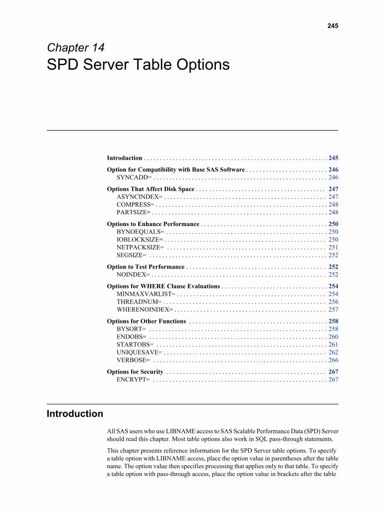
Chapter 14SPD Server Table Options

Introduction . . . . . . . . . . . . . . . . . . . . . . . . . . . . . . . . . . . . . . . . . . . . . . . . . . . . . . . . . 245

Option for Compatibility with Base SAS Software . . . . . . . . . . . . . . . . . . . . . . . . . 246SYNCADD= . . . . . . . . . . . . . . . . . . . . . . . . . . . . . . . . . . . . . . . . . . . . . . . . . . . . . . 246

Options That Affect Disk Space . . . . . . . . . . . . . . . . . . . . . . . . . . . . . . . . . . . . . . . . 247ASYNCINDEX= . . . . . . . . . . . . . . . . . . . . . . . . . . . . . . . . . . . . . . . . . . . . . . . . . . 247COMPRESS= . . . . . . . . . . . . . . . . . . . . . . . . . . . . . . . . . . . . . . . . . . . . . . . . . . . . . 248PARTSIZE= . . . . . . . . . . . . . . . . . . . . . . . . . . . . . . . . . . . . . . . . . . . . . . . . . . . . . . 248

Options to Enhance Performance . . . . . . . . . . . . . . . . . . . . . . . . . . . . . . . . . . . . . . . 250BYNOEQUALS= . . . . . . . . . . . . . . . . . . . . . . . . . . . . . . . . . . . . . . . . . . . . . . . . . . 250IOBLOCKSIZE= . . . . . . . . . . . . . . . . . . . . . . . . . . . . . . . . . . . . . . . . . . . . . . . . . . 250NETPACKSIZE= . . . . . . . . . . . . . . . . . . . . . . . . . . . . . . . . . . . . . . . . . . . . . . . . . 251SEGSIZE= . . . . . . . . . . . . . . . . . . . . . . . . . . . . . . . . . . . . . . . . . . . . . . . . . . . . . . . 252

Option to Test Performance . . . . . . . . . . . . . . . . . . . . . . . . . . . . . . . . . . . . . . . . . . . 252NOINDEX= . . . . . . . . . . . . . . . . . . . . . . . . . . . . . . . . . . . . . . . . . . . . . . . . . . . . . . 252

Options for WHERE Clause Evaluations . . . . . . . . . . . . . . . . . . . . . . . . . . . . . . . . . 254MINMAXVARLIST= . . . . . . . . . . . . . . . . . . . . . . . . . . . . . . . . . . . . . . . . . . . . . . 254THREADNUM= . . . . . . . . . . . . . . . . . . . . . . . . . . . . . . . . . . . . . . . . . . . . . . . . . . 256WHERENOINDEX= . . . . . . . . . . . . . . . . . . . . . . . . . . . . . . . . . . . . . . . . . . . . . . . 257

Options for Other Functions . . . . . . . . . . . . . . . . . . . . . . . . . . . . . . . . . . . . . . . . . . . 258BYSORT= . . . . . . . . . . . . . . . . . . . . . . . . . . . . . . . . . . . . . . . . . . . . . . . . . . . . . . . 258ENDOBS= . . . . . . . . . . . . . . . . . . . . . . . . . . . . . . . . . . . . . . . . . . . . . . . . . . . . . . . 260STARTOBS= . . . . . . . . . . . . . . . . . . . . . . . . . . . . . . . . . . . . . . . . . . . . . . . . . . . . . 261UNIQUESAVE= . . . . . . . . . . . . . . . . . . . . . . . . . . . . . . . . . . . . . . . . . . . . . . . . . . 262VERBOSE= . . . . . . . . . . . . . . . . . . . . . . . . . . . . . . . . . . . . . . . . . . . . . . . . . . . . . . 266

Options for Security . . . . . . . . . . . . . . . . . . . . . . . . . . . . . . . . . . . . . . . . . . . . . . . . . 267ENCRYPT= . . . . . . . . . . . . . . . . . . . . . . . . . . . . . . . . . . . . . . . . . . . . . . . . . . . . . . 267

IntroductionAll SAS users who use LIBNAME access to SAS Scalable Performance Data (SPD) Servershould read this chapter. Most table options also work in SQL pass-through statements.

This chapter presents reference information for the SPD Server table options. To specifya table option with LIBNAME access, place the option value in parentheses after the tablename. The option value then specifies processing that applies only to that table. To specifya table option with pass-through access, place the option value in brackets after the table

245

name. The option value then specifies processing that applies only to that table. The SPDServer table options that follow are grouped by the function of their default value.

When using the options in this chapter, remember that if a table option is used subsequentto a LIBNAME option or macro variable, the value of the table option takes precedence.

Option for Compatibility with Base SAS Software

SYNCADD=Specifies when appending to a table whether to apply a single or multiple rows at a time.

Syntax

SYNCADD=YES|NO

Default

NO

Corresponding Macro Variable

SPDSSADD

Related Table Option

UNIQUESAVE=

Arguments

YESimitates the behavior of the Base SAS engine, applying a single row at a time(synchronously).

NOappends multiple rows at a time (asynchronously).

Description

When SYNCADD= is set to YES, processing performance becomes slower. Use this settingonly in order to force the server's append processing to be compatible with Base SASsoftware processing. That is, when the server encounters a row with a non-unique value,to cancel the append operation, back out the transactions just added, and leave the originaltable on disk.

Example

In this example, when executing the first INSERT statement, PROC SQL permits insertionof the values 'rollback1' and 'rollback2' because the row additions to table A are performedasynchronously. PROC SQL does not get the true completion status at the time it adds arow.

When executing the second INSERT statement, PROC SQL performs a rollback on theINSERT, upon encountering the Add error on 'nonunique', and deletes the rows 'rollback3'and 'rollback4'.

data a; input z $ 1-20 x y; list;

datalines;

246 Chapter 14 • SPD Server Table Options

one 1 10two 2 20three 3 30four 4 40five 5 50;

PROC SQL sortseq=ascii exec noerrorstop;create unique index comp on a (x, y);insert into a values('rollback1', -80, -80) values('rollback2',-90, -90) values('nonunique', 2, 20);

insert into a(syncadd=yes) set z='rollback3', x=-60, y=-60 set z='rollback4', x=-70, y=-70 set z='nonunique', x=2, y=20; quit;

Options That Affect Disk Space

ASYNCINDEX=Specifies when creating multiple indexes on an SPD Server table whether to create theindexes in parallel.

Syntax

ASYNCINDEX=YES|NO

Default

NO


SPDSIASY

Arguments

YEScreates the indexes in parallel.

NOcreates a single index at a time.

Description

SPD Server can create multiple indexes for a table at the same time. To do this, it launchesa single thread for each index created, and then processes the threads simultaneously.Although creating indexes in parallel is much faster, the default for this option is NO. Thereason is because parallel creation requires additional sort work space which might not beavailable.

For a complete description of the benefits and tradeoffs of creating multiple indexes inparallel, see“SPDSIASY=” on page 215 in the SAS SPD Server 4.5: User's Guide.

Example

ASYNCINDEX= 247

Since the disk work space required for parallel index creation is available, specify for SPDServer to create, in parallel, the X, Y, and COMP indexes for table A.

PROC DATASETS lib=mydatalib; modify a(asyncindex=yes); index create x; index create y; index create comp=(x y); quit;

COMPRESS=Compresses SPD Server tables on disk.

Syntax

COMPRESS=YES|NO

Default

NO

Use in Conjunction with Table Option

IOBLOCKSIZE=


SPDSDCMP

Arguments

YESperforms the run-length compression algorithm SPDSRLLC.

NOperforms no table compression.

Description

When COMPRESS= is assigned YES, SPD Server compresses newly created tables by'blocks' based on the algorithm specified. To control the amount of compression, use thetable option IOBLOCKSIZE=. This option specifies the number of rows that you want tostore in the block.

Note: Once a compressed table is created, you cannot change its block size. To resize theblock, you must PROC COPY the table to a new table, setting IOBLOCKSIZE= to theblock size desired for the output table.

PARTSIZE=Specifies the size of an SPD Server table partition.

Syntax

PARTSIZE=n

Default

16 Megabytes



SPDSSIZE=

Affected by LIBNAME option

DATAPATH=

Arguments

nis the size of the partition in megabytes.

Description

Specifying PARTSIZE= forces the software to partition (split) SPD Server tables at thegiven size. The actual size is computed to accommodate the largest number of rows thatwill fit in the specified size of n Mbytes.

Use this option to improve performance of WHERE Clause evaluation on non-indexedtable columns and on SQL GROUP_BY processing. By splitting the data portion of aScalable Platform Data Server table at fixed-sized intervals, the software can introduce ahigh degree of scalability for these operations. The reason: it can launch threads in parallelto perform the evaluation on different partitions of the table, without the threat of file accesscontention between the threads. There is, however, a price for the table splits: an increasednumber of files, which are required to store the rows of the table.

Ultimately, scalability limits using PARTSIZE= depend on how you structureDATAPATH=, a LIBNAME option discussed in the documentation on “SPD ServerLIBNAME Options ” on page 221. Specifically, the limits depend on how you configureand spread the DATAPATH= file systems across striped volumes. You should spread eachindividual volume's striping configuration across multiple disk controllers/SCSI channelsin the disk storage array. The goal for the configuration is, at the hardware level, tomaximize parallelism during data retrieval.

The PARTSIZE= specification is limited by MINPARTSIZE=, an SPD Server parametermaintained by the SPD Server administrator. MINPARTSIZE= ensures that an over-zealous SAS user does not create arbitrarily small partitions, thereby generating a largenumber of files. The default for MINPARTSIZE= is 16 Mbytes and probably should notbe lowered much beyond this value.

Note: The PARTSIZE value for a table cannot be changed after a table is created. Tochange the PARTSIZE, you must PROC COPY the table and use a different PARTSIZEoption setting on the new (output) table.

Example

Using PROC SQL, extract a set of rows from an existing table to create a non-indexed tablewith a partition size of 32 Mbytes in a SAS job:

PROC SQL;create table SPDSCEN.HR80SPDS(partsize=32) as select state, age, sex, hour89, industry, occup from SPDSCEN.PRECS where hour89 > 40;quit;

PARTSIZE= 249

Options to Enhance Performance

BYNOEQUALS=Specifies the output order of table rows with identical values for the BY column.

Syntax

BYNOEQUALS=YES | NO

Arguments

YESdoes not guarantee the output order of table rows with identical values in a BY clause.

NOguarantees the output order of table rows with identical values in a BY clause will bethe relative table position of the rows from the input table. This is the default.

Example

Specify for SPD Server in the ensuing BY-column operation to output rows with identicalvalues in the key column randomly.

data sport.racquets(index=(string)); input raqname $20. @22 weight @28 balance $2. @32 flex @36 gripsize @42 string $3. @47 price @55 instock; datalines;Solo Junior 10.1 N 2 3.75 syn 50.00 6Solo Lobber 11.3 N 10 5.5 syn 160.00 1Solo Queensize 10.9 HH 6 5.0 syn 130.00 3Solo Kingsize 13.1 HH 5 5.6 syn 140.00 3;

data sport.racqbal(bynoequal=yes); set sport.racquets; by balance;run;

IOBLOCKSIZE=Specifies the number of rows in a block to be stored in or read from an SPD Server table.

Syntax

IOBLOCKSIZE=n

Default


4096

Use in Conjunction with Macro Variable “SPDSDCMP=” on page 214 or Table OptionsCOMPRESS= or ENCRYPT= .

Arguments

nis the size of the block.

Description

The software reads and stores a server table in blocks. IOBLOCKSIZE= is useful oncompressed or encrypted tables. SPD Server software does not use IOBLOCKSIZE= onnoncompressed or nonencrypted tables.

For tables that you compress or encrypt, using either the option COMPRESS= or the macrovariable SPDSDCMP=, the IOBLOCKSIZE= specification determines the number of rowsto include in the block. The specification applies to block compression as well as data I/Oto and from disk. The IOBLOCKSIZE= value affects the table's organization on disk.

When using SPD Server table compression or encryption, specify an IOBLOCKSIZE=value that complements how the data is to be accessed, sequentially or randomly. Sequentialaccess or operations requiring full table scans favor a large block size, for example 64K.In contrast, random access favors a smaller block size, for example 8K.

Example

A huge company mailing list is processed sequentially. Specify a block size forcompression that is optimal for sequential access.

/* IOblocksize set to 64K */data sport.maillist(ioblocksize=65536 compress=yes); input name $ 1-20 address $ 21-57 phoneno $ 58-69 sex $71;

datalines;

Douglas, Mike 3256 Main St., Cary, NC 27511 919-444-5555 MWalters, Ann Marie 256 Evans Dr., Durham, NC 27707 919-324-6786 FTurner, Julia 709 Cedar Rd., Cary, NC 27513 919-555-9045 FCashwell, Jack 567 Scott Ln., Chapel Hill, NC 27514 919-533-3845 MClark, John 9 Church St., Durham, NC 27705 919-324-0390 M;run;

NETPACKSIZE=Specifies the size of the SPD Server network data packet.

Syntax

NETPACKSIZE=size-of-packet

Arguments

size-of-packetis the size of the network packet in bytes.

NETPACKSIZE= 251

Description

This option controls the size of the buffer used for data transfer between SPD Server anda SAS client. The default is 32K bytes. The buffer size is relative to the size of a table row.It cannot be less than the size of a single row. Packet size must be equal to some multipleof the table rows. If it is not, SPD Server rounds up the size specified. For example, if thepacket buffer size is 4096 bytes and the row size is 3072, the software rounds up the buffersize to 6144.

Select a packet size to complement the bandwidth of the network it must travel through.An optimum size will flow the data continuously without significant pauses betweenpackets.

Example

Create a 12K buffer in the memory of the server to send three rows from MYTABLE ineach network packet. (The row size in MYTABLE is 4K.)

data mylib.mytable (netpacksize=12288);

SEGSIZE=Specifies the size of the segment for an index file associated with an SPD Server table.

Syntax

SEGSIZE=number

Arguments

numberis the number of table rows to include in the index segment.

Description

The minimum SEGSIZE= value is 1024 table rows. The default value is 8192 table rows.The size of the index segment corresponds to the structure of the table and cannot bechanged after the table is created.

Example

Specify a segment size of 64K for MYLIB.MYTABLE.

data mylib.mytable (segsize=65536);

Note: Tests show that increasing the size of the segment does not significantly increaseperformance.

Option to Test Performance

NOINDEX=Specifies whether to use the table's indexes when processing WHERE Clauses.

Syntax

NOINDEX=YES|NO

Default

NO


Arguments

YESignores indexes when processing WHERE Clauses.

NOuses indexes when processing WHERE Clauses.

Description

Set NOINDEX= to YES to test the effect of indexes on performance or for specificprocessing. Do not use YES routinely for normal processing.

Example

We created an index for the SEX column but decide to test whether it is necessary for ourPROC PRINT processing. Specify for the server not to use the index.

data sport.maillist; input name $ 1-20 address $ 21-57 phoneno $ 58-69 sex $71;

datalines;

Douglas, Mike 3256 Main St., Cary, NC 27511 919-444-5555 MWalters, Ann Marie 256 Evans Dr., Durham, NC 27707 919-324-6786 FTurner, Julia 709 Cedar Rd., Cary, NC 27513 919-555-9045 FCashwell, Jack 567 Scott Ln., Chapel Hill, NC 27514 919-533-3845 MClark, John 9 Church St., Durham, NC 27705 919-324-0390 M;

PROC DATASETS lib=sport nolist; modify maillist; index create sex; quit;

/*Turn on the macro variable SPDSWDEB *//* to show that the index is not used *//* used during the table processing. */

%let spdswdeb=YES;

title All Females from Current Mailing List;PROC PRINT data=sport.maillist(noindex=yes);where sex=F;run;

NOINDEX= 253

Options for WHERE Clause Evaluations

MINMAXVARLIST=Creates an index that documents the minimum and maximum values of specified variables.SPD Server WHERE Clause evaluations use MINMAXVARLIST= indexes to include oreliminate member tables in an SPD Server dynamic cluster table from SQL evaluationscans..

Syntax

MINMAXVARLIST=(varname1, varname2, ... , varnameN)

Arguments

varname1, varname2, ... , varname Nare SPD Server table variable names.

Description

The primary purpose of the MIINMAXVARLIST= table option is for use with SPD Server“SAS Scalable Performance Data (SPD) Server Dynamic Cluster Tables” on page 65 wherespecific members in the dynamic cluster contain a set or range of values, such as sales datafor a given month. When an SPD Server SQL sub setting whereclause specifies specificmonths from a range of sales data, the WHERE planner checks the min/max indexes. Basedon the min/max index information, the SPD Server WHERE planner includes or eliminatesmember tables in the dynamic cluster for evaluation.

MINMAXVARLIST= uses the list of columns you submit to build an index. TheMINMAXVARLIST= index contains only the minimum and maximum values for eachcolumn. The WHERE Clause planner uses the index to filter SQL predicates quickly, andto include or eliminate member tables belonging to the cluster table from the evaluation.

Although the MINMAXVARLIST= table option is primarily intended for use withdynamic clusters, it also works on standard SPD Server tables. MINMAXVARLIST= canhelp reduce the need to create many indexes on a table, which can save valuable resourcesand space.

Example

%let domain=path3 ;%let host=kaboom ;%let port=5201 ;

libname &domain sasspds "&domain" server=&host..&port user='anonymous' ;

/* Create three tables called *//* xy1, xy2, and xy3. */

data &domain..xy1(minmaxvarlist=(x y)); do x = 1 to 10; do y = 1 to 3; output; end;end;


run;



/* Create a dynamic cluster table *//* called cluster_table out of *//* new tables xy1, xy2, and xy3 */

PROC SPDO library=&domain ; cluster create cluster_table mem=xy1 mem=xy2 mem=xy3 maxslot=10;quit;

/* Enable WHERE evaluation to see *//* how the SQL planner selects *//* members from the cluster. Each *//* member is evaluated using the *//* min-max index. */

%let SPDSWDEB=YES;

/* The first member has true rows */


/* Examine the other tables */

PROC PRINT data=&domain..cluster_table ; where x eq 3 and y eq 3 ;run;

MINMAXVARLIST= 255


PROC PRINT data=&domain..cluster_table ; where x between 1 and 10 and y eq 3;run;

PROC PRINT data=&domain..cluster_table ; where x between 11 and 30 and y eq 8 ;run;

/* Delete the dynamic cluster table. */

PROC DATASETS lib=&domain nolist; delete cluster_table ;quit ;

THREADNUM=Specifies the number of threads to be used for WHERE Clause evaluations.

Syntax

THREADNUM=n

Default

THREADNUM= is set equal to the value of the MAXWHTHREADS server parameter.

Used in Conjunction with SPD Server Parameter

MAXWHTHREADS


SPDSTCNT=

Arguments

nis the number of threads.

Description

THREADNUM= allows you to specify the thread count the SPD Server should use whenperforming a parallel WHERE Clause evaluation.

Use this option to explore scalability for WHERE Clause and GROUP_BY evaluations innon-production jobs. If you use this option for production jobs, you are likely to lower thelevel of parallelism that is applied to those clause evaluations.

THREADNUM= works in conjunction with MAXWHTHREADS, a configurable systemparameter. MAXWHTHREADS imposes an upper limit on the consumption of systemresources. The default value of MAXWHTHREADS is dependent on your operatingsystem. Your SPD Server administrator can change the default value forMAXWHTHREADS.


If you do not use THREADNUM=, the software provides a default thread number, up tothe value of MAXWHTHREADS as required. If you use THREADNUM=, the value thatyou specify is also constrained by the MAXWHTHREADS value.

The THREADNUM= value applies both to parallel table scans (EVAL2 strategy), parallelindexed evaluations (EVAL1 strategy), parallel BY-clause processing, and parallelGROUP_BY evaluations. The SPD Server User's Guide Help section on Optimizing SPDServer Performance, contains more information about “Optimizing WHERE clauses” onpage 177.

Example

The SPD Server administrator set MAXWHTHREADS=128 in the SAS ScalablePerformance Data (SPD) Server's parameter file. Explore the effects of parallelism on agiven query by using the following SAS macro:

%macro dotest(maxthr);%do nthr=1 %to &maxthr data _null_; set SPDSCEN.PRECS(threadnum=&nthr); WHERE occup='022' and state in('37','03','06','36'); run;%mend dotest;

WHERENOINDEX=Specifies a list of indexes to exclude when making WHERE Clause evaluations.

Syntax

WHERENOINDEX=(name1 name2...)

Arguments

(name1 name2...)a list of index names that you want to exclude from the WHERE planner.

Example

We have a table PRECS with indexes defined as follows:

PROC DATASETS lib=spdscen;modify precs(bitindex=(hour89));index create stser=(state serialno) occind=(occup industry) hour89;quit;

When evaluating the next query, we want the SPD Server to exclude from considerationindexes for both the STATE and HOUR89 columns.

In this case, we know that our AND combination of the predicates for the OCCUP andINDUSTRY columns will produce a very small yield. Few rows satisfy the respectivepredicates. To avoid the extra index I/O (machine time) that the query requires for a full-indexed evaluation, use the following SAS code:

WHERENOINDEX= 257

PROC SQL;create table hr80spds as select state, age, sex, hour89, industry, occup from spdscen.precs(wherenoindex=(stser hour89)) where occup='022' and state in('37','03','06','36') and industry='012' and hour89 > 40;quit;

Note: Specify index names in the WHERENOINDEX list, not the column names. Theexample excludes both the composite index for the STATE column STSER and thesimple index HOUR89 from consideration by the WHINIT WHERE planner.

Options for Other Functions

BYSORT=Perform an implicit automatic sort when SPD Server encounters a BY clause for a giventable.

Syntax

BYSORT=YES | NO

Arguments

YESsorts the data based on the BY columns and returns the sorted data to the SAS client.This powerful capability means that the user does not have to sort data using a PROCSORT statement before using a BY clause.

NOdoes not sort the data based on the BY columns. This might be desirable if a DATAstep BY clause has a GROUPFORMAT option or if a PROC step reports grouped andformatted data.

Description

The default is YES. The NO argument means the table must have been previously sortedby the requested BY columns. The NO argument allows grouped data to maintain theirprecise order in the table. A YES argument groups the data correctly but possibly in adifferent order from the order in the table.

Example 1 - Group Formatting with BYSORT=

libname sport sasspds 'mylib' host='samson' user='user19' passwd='dummy2';


PROC FORMAT; value dollars 0-99.99="low" 100-199.99="medium" 200-1000="high";run;

data sport.racquets; input raqname $20. @22 weight @28 balance $2. @32 flex @36 gripsize @42 string $3. @47 price @55 instock;

datalines;Solo Junior 10.1 N 2 3.75 syn 50.00 6Solo Lobber 11.3 N 10 5.5 syn 160.00 1Solo Queensize 10.9 HH 6 5.0 syn 130.00 3Solo Kingsize 13.1 HH 5 5.6 syn 140.00 3;

PROC PRINT data=sport.racquets (bysort=yes); var raqname instock; by price; format price dollars.;title 'Solo Brand Racquets by Price Level';run;

Output 14.1 Report Output with BYSORT=

Solo Brand Racquets by Price Level

---------------------------- Price=low ---------------------------

OBS RAQNAME INSTOCK

1 Solo Junior 6

-------------------------- Price=medium --------------------------

OBS RAQNAME INSTOCK

3 Solo Queensize 3

4 Solo Kingsize 3

2 Solo Lobber 1

Example 2 - Group Formatting without BYSORT=

PROC PRINT data=sport.racquets (bysort=no);

BYSORT= 259

var raqname instock; by price; format price dollars.;title 'Solo Brand Racquets by Price Level';run;

Output 14.2 Report Output without BYSORT=

Solo Brand Racquets by Price Level

---------------------------- Price=low ---------------------------

OBS RAQNAME INSTOCK

1 Solo Junior 6

-------------------------- Price=medium --------------------------

OBS RAQNAME INSTOCK

2 Solo Lobber 1

3 Solo Queensize 3

4 Solo Kingsize 3

ENDOBS=Specifies the end row (observation) number in a user-defined range for the processing ofa given table.

Syntax

ENDOBS=n

Arguments


Description

By default, SPD Server processes the entire table unless the user specifies a range of rowswith the STARTOBS= and ENDOBS= options. If the STARTOBS= option is used withoutthe ENDOBS= option, the implied value of ENDOBS= is the end of the table. When bothoptions are used together, the value of ENDOBS= must be greater than STARTOBS=.

In contrast to the Base SAS software options FIRSTOBS= and OBS=, the STARTOBS=and ENDOBS= SPD Server options can be used for WHERE Clause processing in additionto table input operations.

Example

Print only rows 2-4 of the table INVENTORY.OLD_AUTOS.

libname inventory sasspds 'conversion_area' server=husky.5105 user='siteusr1' prompt=yes;


data inventory.old_autos; input year $4. @6 manufacturer $12. model $10. body_style $5. engine_liters @39 transmission_type $1. @41 exterior_color $10. options $10. mileage conditon;

datalines;1971 Buick Skylark conv 5.8 A yellow 00000001 143000 21982 Ford Fiesta hatch 1.2 M silver 00000001 70000 31975 Lancia Beta 2door 1.8 M dk blue 00000010 80000 41966 Oldsmobile Toronado 2door 7.0 A black 11000010 110000 31969 Ford Mustang sptrf 7.1 M red 00000111 125000 3;

PROC PRINT data=inventory.old_autos (startobs=2 endobs=4);run;

Output 14.3 Data in the Printed Output

1982 Ford Fiesta hatch 1.2 M silver 00000001 70000 3

1975 Lancia Beta 2door 1.3 M dk blue 00000010 80000 4

1966 Oldsmobile Toronado 2door 7.0 A black 11000010 110000 3

STARTOBS=Specifies the start row (observation) number in a user-defined range for the processing ofa given table.

Syntax

STARTOBS=n

Arguments


Description

By default, SPD Server processes the entire table unless the user specifies a range of rowswith the STARTOBS= and ENDOBS= options. If the ENDOBS= option is used withoutthe STARTOBS= option, the implied value of STARTOBS= is 1. When both options areused together, the value of STARTOBS= must be less than ENDOBS=.

STARTOBS= 261

In contrast to the Base SAS software options FIRSTOBS= and OBS=, the STARTOBS=and ENDOBS= SPD Server options can be used for WHERE Clause processing in additionto table input operations.

Example

Print only rows 2-4 of the table INVENTORY.OLD_AUTOS.

libname inventory sasspds 'conversion_area' server=husky.5105 user='siteusr1' prompt=yes;

data inventory.old_autos; input year $4. @6 manufacturer $12. model $10. body_style $5. engine_liters @39 transmission_type $1. @41 exterior_color $10. options $10. mileage conditon;

datalines;1971 Buick Skylark conv 5.8 A yellow 00000001 143000 21982 Ford Fiesta hatch 1.2 M silver 00000001 70000 31975 Lancia Beta 2door 1.8 M dk blue 00000010 80000 41966 Oldsmobile Toronado 2door 7.0 A black 11000010 110000 31969 Ford Mustang sptrf 7.1 M red 00000111 125000 3;

proc print data=inventory.old_autos (startobs=2 endobs=4);run;

UNIQUESAVE=Specifies to save rows with non-unique key values (the rejected rows) to a separate tablewhen appending data to tables with unique indexes.

Syntax

UNIQUESAVE=YES|NO|REP

Default

NO

Complements the Table Option

SYNCADD=

Used in Conjunction with Macro Variable

SPDSUSDS=

Corresponding Macro Variable:

SPDSUSAV=

Arguments


YESwrites rejected rows to a separate, system-created table file which can be accessed bya reference to the macro variable SPDSUSDS=.

NOdoes not write rejected rows to a separate table, that is, ignores non-unique key values.

REPwhen updating a master table from a transaction table, where the two tables shareidentical variable structures, the UNIQUESAVE=REP option replaces the row updatedrow in the master table instead of appending a row to the master table. The REP optiononly functions in the presence of a /UNIQUE index on the MASTER table. Otherwisethe REP setting is ignored..

Description

SYNCADD= is defaulted to NO. When NO, table appends are 'pipelined', meaning thatthe server data is sent in a stream a block at a time. (See table option NETPACKSIZE=.)While pipelining is faster than a synchronous append, SAS reports the results of the appendoperation differently for these two modes.

When applying only a single row (SYNCADD=NO), SAS returns a status code for eachADD operation. The application can determine the next action based on the status value.If a row is rejected due to containing a non-unique value for a unique index, the user receivesa status message. In contrast, when data is pipelined (SYNCADD=YES), SAS returns astatus code only after all the rows are applied to a table. As a consequence, the user doesnot know which rows have been rejected.

To enjoy the performance of data pipelining but still retain the rejected rows, use theUNIQUESAVE= option. When set to YES, SPD Server will save any rows that are rejectedto a hidden SAS table.

When using this option, SAS returns the name of the hidden table containing the rejectedrows in the macro variable SPDSUSDS. If you want to report the contents of the table,reference “SPDSUSDS=” on page 203 .

Note: If SYNCADD= YES is set, data pipelining is overridden and the data is processedsynchronously. In this situation, the UNIQUESAVE= option is not relevant and, if set,is ignored.

Example 1

We want to append two tables, NAMES2 and NAMES3, which contain employees' names,to the NAMES1 table. Before performing our append, we create an index on the NAMEcolumn in NAMES1, declaring the index unique.

Specify for SAS Scalable Performance Data (SPD) Server, during the append operation,to store rows found with duplicate employee names to a separate table file generated bythe macro variable SPDSUSDS=.

Use a %PUT statement to display the table name for SPDSUSDS=. Then request a printoutof the duplicate rows to review later.

data employee.names1;input name $ exten;datalines;Jill 4344Jack 5589Jim 8888Sam 3334;run;

UNIQUESAVE= 263

data employee.names2;input name $ exten;datalines;Jack 4443Ann 8438Sam 3334Susan 5321Donna 3332;run;

data employee.names3;input name $ exten;datalines;Donna 3332Jerry 3268Mike 2213;run;

PROC DATASETS lib=employee nolist; modify names1; index create name/unique;quit;

PROC APPEND data=employee.names2 out=employee.names1(uniquesave=yes); run;

title 'The NAMES1 table with unique names from NAMES2';

PROC PRINT data=employee.names1;run;


title 'Duplicate (non-unique) name rows found in NAMES2';

PROC PRINT data=&spdsusds;run;

PROC APPEND data=employee.names3 out=employee.names1(uniquesave=yes);run;

The SAS log provides the messages:

WARNING: Duplicate values not allowed on index NAME for file EMPLOYEE.NAMES1. (Occurred 2 times.)NOTE: Duplicate records have been stored in file EMPLOYEE._30E3FD5.

And, an extract from our PROC PRINT shows:


The NAMES1 table with unique names from NAMES2

OBS NAME EXTENs

1 Jill 4344 2 Jack 5589 3 Jim 8888 4 Sam 3334 5 Ann 8438 6 Susan 5321 7 Donna 3332

Duplicate (non-unique) name rows found in NAMES2

OBS NAME EXTEN XXX00000

1 Jack 4443 NAME 2 Sam 3334 NAME

Example 2

Use the UNIQUESAVE=REP option to perform an update / append case using PROCAPPEND instead of a DATA step:

* A MASTER table to update. ID *//* will get a UNIQUE index */

DATA SPDS.MASTER; INPUT ID VALUE $; CARDS; 1 one 2 two 3 three ;

PROC DATASETS LIB=SPDS; MODIFY MASTER; INDEX CREATE ID/UNIQUE; QUIT;

/* A transaction table TRANS to use to */ /* drive update/appends to MASTER */

DATA SPDS.TRANS; INPUT ID VALUE $; 1 ONE 3 THREE 4 FOUR 4 FOUR* ;

/* Use of UNIQUESAVE=REP to update/append */ /* TRANS rows to MASTER based on whether */ /* TRANS records have an ID column that */ /* matches an existing row from the MASTER */ /* table. Update MASTER rows with a match, */

UNIQUESAVE= 265

/* otherwise append TRANS row to MASTER */

PROC APPEND DATA=SPDS.TRANS OUT=SPDS.MASTER(UNIQUESAVE=REP); run;

Output of the resulting MASTER table would look like:

Obs ID VALUE

1 1 ONE 2 2 two 3 2 THREE 4 4 FOUR*

VERBOSE=Provides details of all indexes and ACL information associated with an SPD Server table.

Syntax

VERBOSE= YES | NO

Arguments

YESrequests detail information for the indexes, ACLs, and other SPD Server table values.This argument must be used with the CONTENTS procedure.

NOsuppresses detail information for the indexes, ACLs, and other SPD Server table values.This is the default.

Example

Request details of all the indexes for the table TEMP1 in the domain SPDS45.

PROC CONTENTS data=SPDS45 (verbose=yes);run;


The CONTENTS Procedure

Data Set Name SPDS45.TEMP1 Observations 1000Member Type DATA Variables 2Engine SASSPDS Indexes 2Created Tuesday, May 10, 2005 10:00:02 AM Observation Length 16Last Modified Tuesday, May 10, 2005 11:01:36 AM Deleted Observations 0Protection Compressed NOData Set Type Sorted NOLabelData Representation DefaultEncoding Default

Engine / Host Dependent Information

Blocking Factor (obs/block) 2047 ACL Entry NO ACL User Access(R,W,A,C) (Y,Y,Y,Y) ACL User Name ANONYMOU ACL Owner Name ANONYMOU Data Set is Ranged NO Alphabetic List of Index Info . Bitmap index (No Global Index ) i Keyvalue (Min) 1 Keyvalue (Max) 100 # of Discrete values 100 Bitmap index (No Global Index ) j Keyvalue (Min) 1 Keyvalue (Max) 10 # of Discrete values 10 Data Partsize 16777216

Alphabetic List of Variables and Attributes

* Variable Type Len

1 i Num 8 2 j Num 9

Alphabetic List of Indexes and Attributes

# of Unique * Index Values

1 i 100 2 j 10

Options for Security

ENCRYPT=Encrypts SPD Server tables on disk. Encryption is a security mechanism that protects tablecontents from users who have system access to raw SPD Server tables. Access to tables is

ENCRYPT= 267

normally controlled by SPD Server ACLs. The SPD Server Administrator's Guide containsdetailed information about using SPD Server ACLs to control access to tables.

When the ENCRYPT= option setting is set to YES, SPD Server encrypts newly createdtables by blocks. To control the amount of encryption per block, use the table optionIOBLOCKSIZE=. The IOBLOCKSIZE= option specifies the number of rows to beencrypted in each block.

Syntax

ENCRYPT= YES | NO

Arguments

YESencrypts the data set. The encryption method uses passwords. At a minimum, you mustspecify the READ= or the PW= data set option at the same time that you specify anENCRYPT=YES option setting.

NOno table encryption is performed. NO is the default setting for the ENCRYPT= option.

Usage Notes

1. Depending on your query patterns, increasing or decreasing the block size can affectperformance.

2. SPD Server does not encrypt table indexes or metadata. Only table row data areencrypted.

3. To encrypt SPD tables with pass-through SQL, use only the READ= or PW= tableoption. With pass-through SQL, ENCRYPT=YES is implied with these options.

4. To access an encrypted table, the user must have appropriate ACL permissions to thetable and must provide the encryption key via the READ= or PW= table option.

5. Encrypting an SPD Server table provides security from users that have system accessto dump raw SPD Server tables. The section on Security in the SPD ServerAdministrator's Guide contains more information about how to controll system accessto SPD Server tables.


Chapter 15SPD Server Formats andInformats

Introduction . . . . . . . . . . . . . . . . . . . . . . . . . . . . . . . . . . . . . . . . . . . . . . . . . . . . . . . . . 269

Formats . . . . . . . . . . . . . . . . . . . . . . . . . . . . . . . . . . . . . . . . . . . . . . . . . . . . . . . . . . . . 269List of Formats . . . . . . . . . . . . . . . . . . . . . . . . . . . . . . . . . . . . . . . . . . . . . . . . . . . . 269Formats Example: . . . . . . . . . . . . . . . . . . . . . . . . . . . . . . . . . . . . . . . . . . . . . . . . . . 271

User-Defined Formats Example . . . . . . . . . . . . . . . . . . . . . . . . . . . . . . . . . . . . . . . . 271

Informats . . . . . . . . . . . . . . . . . . . . . . . . . . . . . . . . . . . . . . . . . . . . . . . . . . . . . . . . . . . 275

IntroductionSAS Scalable Performance Data (SPD) Server supports some of the more commonly usedSAS format and informats. Use these in your SQL pass-through code when you want SASScalable Performance Data (SPD) Server to associate a data set variable with a specificformat.

A general reminder about formats: A format is applied to data set variables as it is writtenout. Informats are applied as the data set variable is being read.

Formats

List of Formats• $ -- Writes standard character data

• $BINARY -- Converts character values to binary representation

• $CHAR -- Writes standard character data

• $HEX -- Converts character values to hexadecimal representation

• $OCTAL -- Converts character values to octal representation

• $QUOTE -- Converts character values to quoted strings

• $VARYING -- Writes varying length values

• BEST -- SAS Scalable Performance Data (SPD) Server system chooses best notation

• BINARY -- Converts numeric values to binary representation

269

• COMMA -- Writes numeric values with commas and decimal points

• COMMAX -- Writes numeric values with commas and decimal points (European style)

• DATE -- Writes date values (ddmmmyy)

• DATETIME -- Writes date time values (ddmmmyy:hh:mm:ss.ss)

• DAY -- Writes day of month

• DDMMYY -- Writes date values (ddmmyy)

• DOLLAR -- Writes numeric values with dollar signs, commas, and decimal points

• DOLLARX -- Writes numeric values with dollar signs, commas, and decimal points(European style)

• DOWNAME -- Writes name of day of the week

• E -- Writes scientific notation

• F -- Writes scientific notation

• FRACT -- Converts values to fractions

• HEX -- Converts real binary (floating-point) numbers to hexadecimal representation

• HHMM -- Writes hours and minutes

• HOUR -- Writes hours and decimal fractions of hours

• IB -- Writes integer binary values

• MMDDYY -- Writes date values (mmddyy)

• MMSS -- Writes minutes and seconds

• MMYY -- Writes month and year, separated by a 'M'

• MONNAME -- Writes name of month

• MONTH -- Writes month of year

• MONYY -- Writes month and year

• NEGPAREN -- Displays negative values in parentheses

• OCTAL -- Converts numeric values to octal representation

• PD -- Writes packed decimal data

• PERCENT -- Prints numbers as percentages

• PIB -- Writes positive integer binary values

• QTR -- Writes quarter of year

• RB -- Writes real binary (floating-point) data

• SSN -- Writes Social Security numbers

• TIME -- Writes hours, minutes, and seconds

• TOD -- Writes the time portion of datetime values

• w.d -- Writes standard numeric data

• WEEKDATE -- Writes day of week and date (day-of-week, month-name dd, yy)

• WEEKDATX -- Writes day of week and date (day-of-week, dd month-name yy)

• WEEKDAY -- Writes day of week

270 Chapter 15 • SPD Server Formats and Informats

• WORDDATE -- Writes date with name of month, day, and year (month-name dd,yyyy)

• WORDDATX -- Writes date with day, name of month, and year (dd month-name yyyy)

• WORDF -- Converts numeric values to words

• WORDS -- Converts numeric values to words (fractions as words)

• YEAR -- Writes year part of date value

• YYMM -- Write year and month, separated by a 'M'

• YYMMDD -- Writes day values (yymmdd)

• YYMON -- Writes year and month abbreviation

• YYQ -- Writes year and quarter, separated by a 'Q'

• Z -- Writes leading 0s

• ZD -- Writes data in zoned decimal format

Note: Formats which begin with a '$' sign are character formats. Otherwise the formataccepts numeric values.

Formats Example:Use the dollar. format to convert numeric sales figures into dollar values. Suppose you havean SPD Server data set saleswith a single numeric variable salesite representing the totalsales for a given site. Using SQL pass-through, create a new data set containing the salesin dollar format.

PROC SQL;connect to sasspds (dbq='tmp' user='anonymous' host='localhost' serv='5127');

execute(create table money as select salesite format=dollar. from sales)

by sasspds;

quit;

User-Defined Formats ExampleThis example is a sample test job that validates its own configuration to use user-definedformats. When properly configured, user-defined formats will allow columns to beformatted using parallel group-by statements and a WHERE-clause that uses a format tosubset data to the server.

The example provides sample spdsserv.parm and libnames.parm file examples, as wellas code examples that follow the two sample SPD Server configuration files.

User-Defined Formats Example 271

This example is a sample test job that checks the usage of user-defined formats. Whencorrectly set up, user-defined formats will allow formatting of columns in parallel group-by and permits usage of a WHERE-clause that uses a format to subset data.

SPD Server spdsserv.parm file used in the example:

SORTSIZE=8M;INDEX_SORTSIZE=8M;BINBUFSIZE=32K;INDEX_MAXMEMORY=8M;NOCOREFILE;SEQIOBUFMIN=64K;RANIOBUFMIN=4K;NOALLOWMMAP;MAXWHTHREADS=16;WHERECOSTING;RANDOMPLACEDPF;FMTDOMAIN=FORMATS;FMTNAMENODE=d8488 ;FMTNAMEPORT=5200;

SPD Server libnames.parm file used in the example:

libname=tmp pathname=c:\temp;libname=formats pathname=c:\data\formats;

SPD Server example code:

%let domain=tmp; %let host=d8488; %let serv=5200;

/* locking=YES must be specified when using */ /* options fmtsearch=(formats); */

libname formats sasspds 'formats' host=&host; serv=&serv; user='anonymous' locking=YES; libname &domain; sasspds &domain; host=&host; serv=&serv; user='anonymous' IP=YES;

options fmtsearch=(formats);

PROC DATASETS nolist lib=formats memtype=catalog; delete formats; quit ;

/* To create user defined formats, they must be */ /* loaded from the same platform where they are */ /* going to be stored. You cannot use Windows */


/* path specifications to load formats on UNIX */ /* platforms. */

/* Add formats to format domain */

PROC FORMAT lib=formats;value AGEGRP 0-13='Child' 14-17='Adolescent' 18-64='Adult' 65-HIGH='Pensioner';value $GENDER 'F' = 'Female' 'M' = 'Male'; run ;

/* Create a test table with a column that uses */ /* AGEGRP format */

data &domain..fmttest; format age AGEGRP. GENDER $GENDER. id z5.; length GENDER $1; do id=1 to 100; if mod (id,2) = 0 then GENDER = 'F'; else GENDER = 'M'; age=int(ranuni(0)*100); income=age*int(ranuni(0)*1000); output;

end;

run;

/* Use the parallel group-by feature with the */ /* fmtgrpsel option. This groups the data based */ /* on the output format specified in the table. */ /* This will be executed in parallel. */

PROC SQL; connect to sasspds(dbq="&domain"; serv="&serv"; host="&host"; user="anonymous");


execute(reset fmtgrpsel)by sasspds;

title 'Simple Fmtgrpsel Example';

select * from connection to sasspds (select age, count(*) as count

User-Defined Formats Example 273

from fmttest group by age);


quit;

PROC SQL;connect to sasspds(dbq="&domain"; serv="&serv"; host="&host"; user="anonymous");



title 'Format Both Columns Group Select Example';

select * from connection to sasspds (select GENDER format=$GENDER., AGE format=AGEGRP., count(*) as count from fmttest formatted group by GENDER, AGE);


quit;

PROC SQL; connect to sasspds(dbq="&domain"; serv="&serv"; host="&host"; user="anonymous");



title1 'To use Format on Only One Column With Group Select'; title2 'Override Column Format With a Starndard Format';

select * from connection to sasspds (select GENDER format=$1., AGE format=AGEGRP., count(*) as count from fmttest formatted group by GENDER, AGE);



quit;

/* A WHERE-clause that uses a format to subset */ /* data is pushed to the server. If it is not */ /* pushed to the server, the following warning */ /* message will be written to the SAS log: */ /* WARNING: Server is unable to execute the */ /* where clause. */

data temp; set &domain..fmttest; where put (AGE,AGEGRP.) = 'Child'; run;

Informats• $ -- Reads standard character data

• $BINARY -- Converts binary values to character values

• $CB -- Reads standard character data from column-binary files

• $CHAR -- Reads character data with blanks

• $HEX -- Converts hexadecimal data to character data

• $OCTAL -- Converts octal data to character data

• $PHEX -- Converts packed hexadecimal data to character data

• $QUOTE -- Converts quoted strings to character data

• $SASNAME --

• $VARYING -- Reads varying length values

• BEST -- SPD Server system chooses best notation

• BINARY -- Converts positive binary values to integers

• BITS -- Extract bits

• COMMA -- Removes embedded characters (for example $,.)

• COMMAX -- Removes embedded characters (for example $,.) European style

• D -- Reads scientific notation

• DATE -- Reads date values (ddmmmyy)

• DATETIME -- Reads datetime values (ddmmmyy hh:mm:ss.ss)

• DDMMYY -- Reads date values (ddmmyy)

• DOLLAR -- Reads numeric values with dollar signs, commas, and decimal points

• DOLLARX -- Reads numeric values with dollar signs, commas, and decimal points(European style)

• E -- Reads scientific notation

Informats 275

• F -- Reads scientific notation

• HEX -- Converts hexadecimal positive binary values to fixed- or floating-point values

• IB -- Reads integer binary (fixed-point) values

• JULIAN -- Reads Julian dates (yyddd or yyyyddd)

• MMDDYY -- Reads date values (mmddyy)

• MONYY -- Reads month and year date values (mmmyy)

• MSEC -- Reads TIME MIC values

• OCTAL -- Converts octal values to integers

• PD -- Reads packed decimal data

• PDTIME -- Reads packed decimal time of SMF and RMF records

• PERCENT -- Converts percentages into numeric values

• PIB -- Reads positive integer binary (fixed-point) values

• PK -- Reads unsigned packed decimal data

• PUNCH -- Reads whether a row of column-binary data is punched

• RMFSTAMP -- Reads time and date fields of RMF records

• ROW -- Reads a column-binary field down a card column

• SMFSTAMP -- Reads time-date values of SMF records

• TIME -- Reads hours, minutes, and seconds (hh:mm:ss.ss)

• TODSTAMP -- Reads 8-byte time-of-day stamp

• TU -- Reads timer units

• YYMMDD -- Reads date values (yymmdd)

• YYQ -- Reads quarters of the year

Note: Informats which begin with a '$' sign are character informats. Otherwise the informataccepts numeric values.

The SQL procedure itself does not use the INFORMAT= modifier: it stores informats inits table definitions so that other procedures and the DATA step can use the information.SPD Server informats are provided now to allow for forward compatibility with futuredevelopment.


Chapter 16SPD Server NLS Support

Overview of NLS . . . . . . . . . . . . . . . . . . . . . . . . . . . . . . . . . . . . . . . . . . . . . . . . . . . . . 277

Character Encoding Overview . . . . . . . . . . . . . . . . . . . . . . . . . . . . . . . . . . . . . . . . . 278Overview of Character Encoding . . . . . . . . . . . . . . . . . . . . . . . . . . . . . . . . . . . . . . 278What is Character Encoding? . . . . . . . . . . . . . . . . . . . . . . . . . . . . . . . . . . . . . . . . . 278Common Encodings . . . . . . . . . . . . . . . . . . . . . . . . . . . . . . . . . . . . . . . . . . . . . . . . 280

Moving Data across Environments with Different Encodings . . . . . . . . . . . . . . . . 281Transcoding . . . . . . . . . . . . . . . . . . . . . . . . . . . . . . . . . . . . . . . . . . . . . . . . . . . . . . 281How Base SAS Transcodes Data . . . . . . . . . . . . . . . . . . . . . . . . . . . . . . . . . . . . . . 282

Base SAS Encoding Behavior . . . . . . . . . . . . . . . . . . . . . . . . . . . . . . . . . . . . . . . . . . 282Overview of Base SAS Encoding . . . . . . . . . . . . . . . . . . . . . . . . . . . . . . . . . . . . . . 282SAS 9 Output Processing . . . . . . . . . . . . . . . . . . . . . . . . . . . . . . . . . . . . . . . . . . . . 282SAS 9 Input Processing . . . . . . . . . . . . . . . . . . . . . . . . . . . . . . . . . . . . . . . . . . . . . 283Reading and Writing External Files . . . . . . . . . . . . . . . . . . . . . . . . . . . . . . . . . . . . 283

Setting the Encoding for Base SAS Sessions . . . . . . . . . . . . . . . . . . . . . . . . . . . . . . 283

Changing the Encoding for Base SAS Sessions . . . . . . . . . . . . . . . . . . . . . . . . . . . . 284

NLS Support in SPD Server . . . . . . . . . . . . . . . . . . . . . . . . . . . . . . . . . . . . . . . . . . . 285Overview of NLS Support . . . . . . . . . . . . . . . . . . . . . . . . . . . . . . . . . . . . . . . . . . . 285SPD Server NLS Limitations . . . . . . . . . . . . . . . . . . . . . . . . . . . . . . . . . . . . . . . . . 285LIBNAME Option Restrictions: . . . . . . . . . . . . . . . . . . . . . . . . . . . . . . . . . . . . . . . 286

Overview of NLSNLS, or National Language Support, deals both with Internationalization and Localizationof SAS software. Internationalization is the process of designing an application so that itcan be adapted to different languages and regions, without requiring engineering changes.Often the term internationalization is abbreviated as i18n, because there are 18 lettersbetween the first i and the last n. Localization is the process of adapting software for aparticular region or language by adding locale-specific components and translating text.The term localization is often abbreviated as L10n, because there are 10 letters betweenthe L and the n. Translation of user interface, messages, and documentation is a large part(but not all) of localization. Localizers also verify that the formatting of dates, numbers,currencies, and so on, conforms to local requirements.

SAS 9 contains built-in support for NLS character set encoding and locale choices. Usersaccess the NLS encoding and locale choices through various SAS, LIBNAME, and dataset options. SAS Scalable Performance Data (SPD) Server and SAS together offer basic

277

levels of NLS support. This document describes the basic entities of NLS support and howthey are implemented in SPD Server

Character Encoding Overview

Overview of Character EncodingAll input to a computer is represented internally as numbers. The computer assigns anumber to each character -- technically, the number is a binary number (base 2 numberingsystem, consisting of 0s and 1s).

Because most of us don't want to think in binary numbers, computers provide hexadecimal(base 16 numbering system) representation as a shorthand for binary representation. Forexample, for the decimal number 167, it's easier to understand the hexadecimal number A7than the equivalent binary number 10100111. Therefore, you can think of the computer'sinternal numeric representation of all data as a hexadecimal number.

What is Character Encoding?All data that is stored, transmitted, or processed by a computer is in an encoding. Anencoding maps each character to a unique numeric representation. For example:

1. You press a key on a keyboard, like the uppercase letter A.

2. The computer assigns the internal numeric representation, that is, a unique hexadecimalnumber.

3. To display or print the character, the computer uses the font (graphical representation)that matches the numeric representation, that is, the uppercase letter A.

To assign the numeric representation to a character, an encoding uses a code page, whichis an ordered set of characters in which a numeric index (code point value) is associatedwith each character. The position of a character on the code page determines its two-digithexadecimal number. The first digit of the hexadecimal number is determined by thecolumn, and the second digit by the row. For example, the following is the code page forthe Windows Latin1 encoding. The numeric representation for the uppercase A is thehexadecimal number 41, and the numeric representation for the equal sign (=) is thehexadecimal number 3D.

278 Chapter 16 • SPD Server NLS Support

Encoding is the combination of a character set with an encoding method:

• A character set is the repertoire of characters and symbols that are used by a languageor group of languages. A character set includes national characters (which are charactersspecific to a particular nation or group of nations), special characters (such aspunctuation marks), the unaccented Latin characters A-Z, the digits 0-9, and controlcharacters that are needed by the computer.

• An encoding method is the set of rules that are used to assign the numbers to the set ofcharacters that are in an encoding. These rules govern such things as the size of theencoding (number of bits used to store the numeric representation of the character) andthe ranges in the code page where characters are allowed to appear.

When the rules of the encoding method are followed, and numbers are assigned to thecharacters, the result is called an encoding.

An individual character can have different positions in code pages for different encodings,which result in different hexadecimal numbers. For example, the position of the uppercaseletter A in the Wlatin1 code page (shown above) results in the hexadecimal number 41,while in the following Danish EBCDIC code page, the position of the uppercase letter Aresults in the hexadecimal number C1.

What is Character Encoding? 279

Common EncodingsThere are many encodings that address the requirements of different languages. Very fewlanguages use only the 26 characters A through Z of the Latin alphabet. In addition, thereare different encodings to address different operating system standards.

An encoding that represents each character in one byte is a single-byte character set (SBCS).A single-byte character set can be either 7 bits (providing up to 128 characters) or 8 bits(providing up to 256 characters). An example of an 8-bit SBCS is the Latin1 encoding(represents the characters of Western Europe). (Note that the term octet, for theinternational community, is an 8-bit byte. Since a byte is not 8 bits in all computer systems,octet provides an unambiguous term.)

A multiple-byte character set (MBCS) is a mixed-width encoding in which some charactersconsist of more than one byte. For example, the Japanese, Korean, Simplified Chinese, andTraditional Chinese are MBCS encodings. A double-byte character set (DBCS) is a specifictype of an MBCS encoding that includes characters that consist of two bytes.

The following are common encodings:


ASCII (American Standard Code for Information Interchange)is a 7-bit encoding for the United States that provides 128 character combinations. Theencoding contains characters for uppercase and lowercase English, American Englishpunctuation, base 10 numbers, and a few control characters. The set of 128 charactersis the one common denominator that is contained in most encodings, excludingEBCDIC-based encodings. ASCII is used by personal computers.

ISO (International Organization for Standardization) 646 familyis a 7-bit encoding that is an international standard and provides 128 charactercombinations. The ISO 646 family of encodings is like ASCII except for 12 code pointsfor national variants. The 12 national variants represent specific characters needed fora particular language.

EBCDIC (Extended Binary Coded Decimal Interchange Code) familyis an 8-bit encoding that provides 256 character combinations. There are multipleEBCDIC-based encodings. EBCDIC is used on IBM mainframes and most IBMmidrange computers. EBCDIC follows ISO 646 conventions to facilitate translationsbetween itself and 7-bit ASCII-based encodings. Characters A-Z and 0-9 are mappedto the same code points on all EBCDIC code pages, while the rest of the code pointscan be used for special characters and national characters, depending on the encoding.

ISO 8859 family and Windows familyis an 8-bit extension of ASCII that supports all of the ASCII code points and adds 12more, providing 256 character combinations. Latin1, which is officially namedISO-8859-1, is the most frequently used member of the ISO 8859 family of encodings.In addition to the ASCII characters, Latin1 contains accented characters, other lettersneeded for languages of Western Europe, and some special characters.

Unicodeuses two bytes for each character rather than one and provides up to 65,536 charactercombinations. Unicode can handle the scripts of basically all of the world's languages.For example, the Japanese language, which has thousands of characters, uses a 16-bit,multiple-byte character set. There are various forms of Unicode, including UTF-8,UTF-16, and UTF-32.

Moving Data across Environments with DifferentEncodings

TranscodingAlthough it's easy to move data across environments that use the same encoding, it can bemore difficult to move data across environments that use different encodings. When theencoding of a file is incompatible with the computer environment's encoding, transcodingoccurs.

Transcoding is the process of mapping data from one encoding to another, such as mappingdata from an ASCII-based encoding to an EBCDIC-based encoding. Transcoding is nottranslating from one language to another; transcoding is remapping of characters.

For example, consider a file that was created on a UNIX platform that uses the Latin1encoding, then moved to an IBM mainframe that uses the Danish EBCDIC encoding. Whenthe file is processed on the IBM mainframe, the data is remapped from the Latin1 encodingto the Danish EBCDIC encoding. If the data contains a dollar sign ($), the hexadecimalnumber is converted from 24 to 67.

Transcoding 281

Transcoding can occur in the following situations:

• when you move a SAS file from one platform to another and the file's encoding isincompatible with the current session encoding. An example might be moving a SASfile from a z/OS operating environment with an EBCDIC-based encoding to a Windowsoperating environment with an ASCII-based encoding.

• when you share data between two SAS sessions (like in a client/server environment)that have incompatible session encodings.

• when you read and write an external file.

How Base SAS Transcodes DataBase SAS provides transcoding when you move data and applications from oneenvironment to another. To transcode one encoding to another, SAS uses translation tables,like the one that maps Wlatin2 (Windows) to ISO Latin2 (UNIX).

For example, when you

• use the CPORT and CIMPORT procedures to create a transport file, SAS automaticallyuses translation tables to transcode one encoding to another and back again. First, thedata is converted from the source encoding to transport format, then the data isconverted from the transport format to the target encoding.

• process a SAS data set that has an encoding that is different from the current sessionencoding, SAS automatically uses CEDA (cross environment data access) software totranscode data. (CEDA is the same software in SAS that converts a SAS file to thecorrect data representation when you move a file from one platform to another.)

Base SAS Encoding Behavior

Overview of Base SAS EncodingFor Base SAS files (not SPD Server), the encoding support depends on the version of SASthat created the file:

• Data sets created in SAS 9 automatically have an encoding attribute, which is stampedin the descriptor portion of the file.

• Data sets created in SAS 8 do not have an encoding value stamped on the file; they areassumed to be in the session encoding of the host environment.

The NLS features in SPD Server only support encoding from SAS 9.

SAS 9 Output ProcessingFor SAS 9 data sets (not SPD Server), encoding is determined as follows:

• For a new output file, the data is written to the file using the current session encoding.

• For a new output file that is created with the OUTREP= option, which specifies a datarepresentation different from the current session, the data is written to the file using thedefault session encoding for the operating system that is based on the specifiedOUTREP= value.

• For output processing that replaces an existing file, the new file inherits the encodingof the existing file.


• For output processing that replaces an existing file that is from another platform or ifthe existing file has no encoding stamped on it, then the current session encoding isused.

SAS 9 Input ProcessingFor input (read) processing in SAS 9 (not SPD Server), encoding behavior is as follows:

• If the session encoding and the encoding that is stamped on the file are incompatible,the data is transcoded to the session encoding. For example, if the current sessionencoding is ASCII and the encoding that is stamped on the file is EBCDIC, SAStranscodes the data from EBCDIC to ASCII.

• If a file does not have an encoding stamped on it, SAS transcodes the data only if thefile's data representation is different from the current session.

Reading and Writing External FilesSAS reads and writes external files using the current session encoding. SAS assumes thatthe external file is in the same encoding as the session encoding. For example, if you arecreating a new SAS data set by reading an external file, SAS assumes that the file's encodingis the same as the session encoding. If it is not, the data could be written to the new SASdata set incorrectly.

Setting the Encoding for Base SAS SessionsWhen SAS 9 is installed, the Base SAS (not SPD Server) default encoding is host dependentand is determined by the default settings for several SAS system options. Here are threesystem options that you should be familiar with:

ENCODING=establishes the session encoding, which is the encoding that SAS uses to process syntax,process SAS data sets, and read and write external files. The default value is hostdependent; all are SBCS encodings:

Table 16.1 Default Session Encodings

Host Value Description

OpenVMS Latin1 Western (ISO)

z/OS OPEN_ED_1047 OpenEdition EBCDICcp1047-Latin1

UNIX Latin1 Western (ISO)

Windows WLatin1 Western (Windows)

LOCALE=specifies the locale of the SAS session. The locale reflects the local language,conventions, and culture for a particular geographical region. A locale's conventionscan include the formatting of dates, times, and numbers, and printer preferences likepaper size. Specifying a locale also automatically sets the default encoding that

Setting the Encoding for Base SAS Sessions 283

establishes the session encoding; a locale has a common encoding that is used mostoften for a particular operating environment. The default locale is English, and thecommon encodings for English are the defaults above for ENCODING=.

NONLSCOMPATMODE | NLSCOMPATMODEprovides national language compatibility for non-English data processing using nativecharacters. For SAS 9, the default is NONLSCOMPATMODE, which providesconsistency for running SAS on multiple systems. NONLSCOMPATMODE specifiesthat data is to be processed in the encoding that is set by the ENCODING= or LOCALE=system option.

Changing the Encoding for Base SAS Sessions

You can change the session encoding by using the LOCALE= system option, theENCODING= system option, or both. Note that valid values for both options are hostdependent.

Here's how you can set the Base SAS (not SPD Server) session encoding whenNONLSCOMPATMODE is specified:

• You can specify the LOCALE= system option in a configuration file, at SASinvocation, in an OPTIONS statement, or in the SAS System Options window. In SAS9, several NLS-related system options are automatically set, based on the value ofLOCALE=. Most customers will implicitly set encoding with the LOCALE= systemoption.

• You can specify the ENCODING= system option in a configuration file or at SASinvocation.

• Here is how LOCALE= and ENCODING= interact:

• If a value is not specified for ENCODING= (that is, the installation default is set),then specifying a value for LOCALE= sets the encoding based on the LOCALE=value. In addition, values for the following system options are set based on theLOCALE= value: DFLANG=, TRANTAB=, DATESTYLE=, and PAPERSIZE=.

• If a value is specified for ENCODING=, that value sets the session encoding andoverrides LOCALE=.

• If the value specified for LOCALE= is not compatible with the value specified forENCODING=, then the value for LOCALE= is used. A warning message isprovided if ENCODING= and LOCALE= conflict.

• If the DBCS system option is set, which specifies that SAS process DBCS encodings,the values for DBCSLANG= and DBCSTYPE= system options determine the sessionencoding and the locale. These options are used for Asian languages or for English withDBCS extensions.

Here is an example of implicitly setting the Base SAS (not SPD Server) session encodingbased on the specified locale when you invoke SAS:

sas9 -explorer -locale spanish

Here is an example of explicitly setting the Base SAS (not SPD Server) session encodingwith the OPTIONS statement:

options encoding=wlatin2;


T I P Changing encoding for a SAS session does not affect SAS keywords, which remainin English, or SAS log output, which also remains in English.

NLS Support in SPD Server

Overview of NLS SupportSPD Server contains support for a subset of the SAS 9 NLS functions documented above.SPD Server uses encoding and locale currently only on SAS software.

In future releases of SPD Server, the locale identifier information will be used for locale-sensitive case folding and linguistic collation. Case-folding is defined as a process appliedto a sequence of characters, in which those identified as non-uppercase are replaced bytheir uppercase equivalents. Linguistic collation is performing linguistic sorts based onlinguistic sort keys. However, those functions have yet to be implemented in SPD Serverproduction code.

All tables that are produced by SPD Server and SAS inherit the SAS session's defaultencoding and locale settings. By default, SPD Server code expects new tables to follow thecurrent SAS session's encoding and locale. Table updates that append rows or updateexisting rows will perform transcoding to ensure that appended and updated table rowsmatch the existing table encoding.

Wire transfer is in the character set encoding of the SAS session for transfers to and fromthe SPD Server host, unless SPD Server transcoding has been disabled. SPD Servertranscoding is enabled or disabled by inserting a [NO]NLSTRANSCODE statement in theSPD Server spdsserv.parm parameter file.

SPD Server NLS Limitations

Affected DataSPD Server hosts are restricted in the way they handle NLS character strings. SPD Serverhosts are restricted to data that is contained in character columns in data sets and somemetadata structures. The NLS support for SPD Server is functional for only table labelsand variable labels.

Column names, index names, table names, and catalog names are not supported in the SPDServer NLS support. Column names, index names, table names, and catalog names are stilldependent on ASCII support. SPD Server SQL is subject to the NLS same restrictions.

Pass-Through SQLSPD Server pass-through SQL does not support any NLS functions. Pass-through SQLoperates in the encoding and locale of the SAS session that initiates the CONNECT toSASSPDS.

Case Folding and Sort SequencesSPD Server NLS code supports very limited English Latin1 and Polish Latin2 case foldingfor SBCS encodings. UTF8 case folding is limited to the ASCII range of UTF8 encoding.NLS Sort sequences for SPD Server 4.5 are restricted to lexical sorts for all combinations.Linguistic sorting is a subject for future SPD Server releases.

SPD Server NLS Limitations 285

Indexes and OrderingIndexes in SPD Server are created in the table's encoding, and only support lexical ordering.If the client's encoding and locale settings match the SPD Server host table's encoding andlocale settings, index use is unrestricted. Otherwise, index usage is restricted to certainpredicates in WHERE clauses that can be safely interpreted according to the table'sencoding and locale settings. When the client and host table encoding and locale settingsdiffer, the EVAL2 strategy is used to filter predicates that require use of order.

Date and Time RepresentationsSPD Server server-side functions and formats that produce or accept textual date, time, anddate/time representations are not locale-sensitive.

Suppressing TranscodingYou can suppress transcoding in the SPD Server environment by entering the followinginto the spdsserv.parm options:

NONLSTRANSCODE;

If you add the NONLSTRANSCODE option to your spdsserv.parm file, charactertranscoding between the SPD Server host and connected clients is disabled. Disablingcharacter transcoding restricts the types of operations that the SPD Server host performsto operations it can safely perform, where host and client tables share the same encoding.Disabling SPD Server host transcoding assumes that the client will perform any neededtranscoding on the data streams that it sends and receives to match the encoding ofreferenced tables. The SPD Server host setting for NONLSTRANSCODE does not performany actions to deny client access to a host table that has mismatched encoding.

LIBNAME Option Restrictions:The following options are not implemented in the SPD Server NLS functions:

The LIBNAME option

OUTENCODING=<client-server encoding>

is not supported and will produce a WARNING message if submitted to sasspds.

In addition, the related data set option

ENCODING=<client-server encoding>

is supported by the SAS LIBNAME engine for OUTPUT data sets only. Character data isassumed to be in the encoding of the session that initiates the CONNECT to SASSPDSand is normally stored using that encoding. ENCODING= will cause SPD Server totranscode from the SAS session encoding to the specified encoding for storing data. If youspecify ENCODING= for a non OUTPUT data set open, and if the encoding value that youspecify doesn't match the data set's encoding, the data set open will produce a warning:

ENCODING= specified on table open fails to match tableencoding. Option ignored.

The LIBNAME option

TRUNCWARN=YES

Suppresses hard failure on NLS transcoding overflow and character mapping errors. Whenusing the TRUNCWARN=YES LIBNAME option, data integrity can be compromisedbecause significant characters can be lost in this configuration. The default setting is NO,which causes hard read/write stops when transcode overflow or mapping errors areencountered. When TRUNCWARN=YES, and an overflow or character mapping error


occurs, a warning is posted to the SAS log at data set close time if overflow occurs, but thedata overflow is lost.

LIBNAME Option Restrictions: 287

Part 6

Appendix

Chapter 17SPD Server Frequently Asked Questions . . . . . . . . . . . . . . . . . . . . . . . . 291

289

Chapter 17SPD Server Frequently AskedQuestions

SPD Server Frequently Asked Questions . . . . . . . . . . . . . . . . . . . . . . . . . . . . . . . . . 292Does SPD Server support files that are larger than 2 Gigabytes in size? . . . . . . . 292Can I create file systems that are larger than 2 Gigabytes in size? . . . . . . . . . . . . . 292How do SPD Server client and server processes communicate? . . . . . . . . . . . . . . 292How do I know which ports must be surfaced through an Internet firewall? . . . . . 293How does SPD Server interact with multi-homed hosts? . . . . . . . . . . . . . . . . . . . . 294Can I use standard UNIX backup procedures? . . . . . . . . . . . . . . . . . . . . . . . . . . . . 294What do I need to know about SPD Server installation? How

long will it take? . . . . . . . . . . . . . . . . . . . . . . . . . . . . . . . . . . . . . . . . . . . . . . . . . 294Is it necessary to run UNIX SPD Server as root? . . . . . . . . . . . . . . . . . . . . . . . . . . 294What is the SPD Server Name Server, and why do I need it? . . . . . . . . . . . . . . . . 295Does every SPD Server client need a UNIX ID or Windows Networking ID? . . . 295Can an SPD Server host, SPD Server Name Server and an SPD

Server client all run on the same machine? . . . . . . . . . . . . . . . . . . . . . . . . . . . . . 295Can I have multiple SPD Server hosts on the same machine? . . . . . . . . . . . . . . . . 295How do I create LIBNAME domains? . . . . . . . . . . . . . . . . . . . . . . . . . . . . . . . . . . 295How do I specify a LIBNAME domain in SAS? . . . . . . . . . . . . . . . . . . . . . . . . . . 295Is there anything else I have to change to run my existing SAS applications? . . . 296How can I get existing data loaded into an SPD Server table? . . . . . . . . . . . . . . . 296Can SPD Server create indexes in parallel? . . . . . . . . . . . . . . . . . . . . . . . . . . . . . . 297Does SPD Server append indexes in parallel? . . . . . . . . . . . . . . . . . . . . . . . . . . . . 297What are ACLs and how do I use them to control access to data tables? . . . . . . . 297How do I get a list of the SAS macro variables introduced for SPD Server? . . . . 298What about unique indexes? Can I do something to speed appends? . . . . . . . . . . 298What about disk compression for SPD Server tables? . . . . . . . . . . . . . . . . . . . . . . 298What about estimates for disk space consumption when using SPD Server? . . . . 298Transient space for PROC SORT / BY processing . . . . . . . . . . . . . . . . . . . . . . . . 301What should I set WORKPATH= to? . . . . . . . . . . . . . . . . . . . . . . . . . . . . . . . . . . 302How do I, as a LIBNAME domain owner, allow others to create

tables in my domain? . . . . . . . . . . . . . . . . . . . . . . . . . . . . . . . . . . . . . . . . . . . . . . 302How does the system administrator list the access control lists for "user 1"? . . . . 303How do I change existing PROC SQL code that works with

SAS to query SPD Server tables? . . . . . . . . . . . . . . . . . . . . . . . . . . . . . . . . . . . . 304Can I use pass-through async to create multiple indexes on a

single existing table? . . . . . . . . . . . . . . . . . . . . . . . . . . . . . . . . . . . . . . . . . . . . . . 307Can I use pass-through async to create multiple indexes on existing tables? . . . . 308What size increases can I expect for tables that are stored in

domains with BACKUP=YES? . . . . . . . . . . . . . . . . . . . . . . . . . . . . . . . . . . . . . . 308

291

SPD Server Frequently Asked Questions

Does SPD Server support files that are larger than 2 Gigabytes insize?

Yes. SPD Server does so by breaking up larger files into partitions that are smaller than 2Gigabytes. The SPD Server host performs this function automatically and it requires nospecial syntax.

Can I create file systems that are larger than 2 Gigabytes in size?Yes, if you use a volume manager that will let you create file systems greater than 2Gigabytes. SAS recommends this practice.

How do SPD Server client and server processes communicate?An SPD Server client communicates with three SPD Server processes.

When a client issues a LIBNAME assignment to the SPD Server host, the clientcommunicates with the SPD Server name server process using the HOST= and SERV=options that were specified in the LIBNAME connection. The HOST= option specifies thehost system where the SPD Server name server is running, and the SERV= option is thewell-known port number of the SPD Server name server that was specified when thesoftware was started. The SPD Server name server ensures that the domain of theLIBNAME assignment is valid, then returns the HOST= and SERV= option settings to theclient. This ends the interaction of the client with the SPD Server name server for thatLIBNAME assignment. The client will communicate with the SPDSSERV process tocomplete the LIBNAME assignment.

The SPDSSERV process authenticates the USER and PASSWORD portion of theLIBNAME assignment, and validates whether the USER has access to the domain. If theLIBNAME is successfully authenticated, the SPDSSERV process forks and executes auser proxy, the SPDSBASE process, which continues to service all other client requestsfor that LIBNAME connection. Subsequent LIBNAME assignments from the same clientthat are resolved to the same SPD Server user and SPDSSERV context are passed directlyto SPDSBASE for processing without any further SPDSSERV interaction. (No furtherinteraction is required because the authentication is inherited by subsequent LIBNAMEassignments.)

LIBNAME assignments from the same client for a different SPD Server user or LIBNAMEassignments to a domain that is serviced by a different SPDSSERV will result in a newSPDSBASE process to service that LIBNAME assignment.

Connections that use the record-level locking option LOCKING=YES to connect to aserver in any domain are handled differently. All LIBNAME assignments share the sameSPDSBASE record level locking process. When the LOCKING=YES option is in force,instead of forking and executing a new user proxy, the SPDSSERV process initiatescommunication with the shared LOCKING=YES SPDSBASE process and the client.

292 Chapter 17 • SPD Server Frequently Asked Questions

How do I know which ports must be surfaced through an Internetfirewall?

There are two ports that the SPDServer name server uses that you can specify usingcommand line options. The listenport option defines the port that must be used by clients(such as SAS) in LIBNAME and SQL CONNECT statements. The listenport option canalso define the port that an ODBC data source requires to communicate with the SPD Servername server. The operport option defines a second port that is used for various commandcommunications from SPD Server utilities. Either of these ports can be specified usingwell-known port definitions in the operating system's services file, instead of specifyingthem on the command line. In UNIX systems, this is typically the /etc/services file.In the services file, the spdsname specification corresponds to listenport, and thespdsoper setting corresponds to the operport setting. Both of these ports should besurfaced through the firewall.

The SPDSSERV process uses two types of ports. The first type of port is a port thatSPDSSERV uses for local machine communications, internal to SPD Server. The secondtype of ports are ports that must be accessed by SPD Server clients.

Ports in the first category are not discussed here, because they do not need to be visiblebeyond the local machine, and therefore do not need firewall connectivity. There are twoports in the second category. The first port in the second category is the port that is definedby the SPDSSERV listenport command line option that performs LIBNAMEauthentication of the SPD Server user and password, and validates access to the SPD Serverdomain. The second port in the second category is the port that is used for variouscommunications from SPD Server utilities, and is defined by the SPDSSERV -operportcommand line option.

The SPDSSERV listenport and operport specifications are registered in the SPD ServerName Server by the SPDSSERV process when it starts up. Both specifications are returnedto the SPD Server client from the SPD Server Name Server when it maps the LIBNAMEdomain to an SPDSSERV. If you do not specify a listenport or operport in the SPDSSERVcommand line, any port that is available will be used. Both of these ports should be specifiedin the SPDSSERV command line and surfaced through the firewall.

Ports that the SPDSBASE process uses also fall into the two same categories. The first typeof ports is used for local machine communications that are internal to SPD Server. Thesecond type of ports are ports that must be accessed by SPD Server Clients. Like theSPDSSERV process, the SPDSBASE process only cares about the ports that outside clientsneed to access through an Internet firewall.

The way that the SPDSBASE processes use ports is complex and requires a range of portnumbers that are declared using the SPD Server MINPORTNO=/MAXPORTNO= serverparameter specifications. The MINPORTNO= and MAXPORTNO= parameters must bothbe specified in order to define the range of port numbers that are available to communicatewith SPD Server clients, and therefore require access from outside of the firewall. If theSPD Server parameters for MINPORTNO= and MAXPORTNO= are not specified, theSPDSBASE processes will use any port that is available to communicate with the SPDServer client.

How many port numbers need to be set aside for SPDSBASE proxy processes? EachSPDSBASE process produces its own operator port that can be accessed using command-line specifications issued by an SPD Server client. In addition, each SPD Server table thatis opened creates its own port. Each table's port becomes a dedicated data transferconnection that is used to stream data transfers to and from the SPD Server client. SPDServer table ports are normally dynamically assigned, unless the MINPORTNO= andMAXPORTNO= parameters have been specified. If the MINPORTNO= and

How do I know which ports must be surfaced through an Internet firewall? 293

MAXPORTNO= parameters have been specified, SPD Server table ports are assigned fromwithin the specified port range.

Therefore, it follows that the range of ports that is specified for the MINPORTNO= andMAXPORTNO= parameters must take into consideration the peak number of concurrentLIBNAME connections that will be made to the server, as well as the I/O streams that arechanneled between the SPDSBASE processes and the SPD Server clients.

The following ports must be surfaced for access beyond the firewall:

• Two SPD Server name server ports, listenport and operport , as well as any otherports that are identified in SPDSNAME and SPDSOPER services.

• Two SPDSSERV ports: listenport and operport , as well as any other ports that areidentified in SPDSSERV_SAS and SPDSSERV_OPER services.

• Any other ports that are defined in the MINPORTNO= and MAXPORTNO= range thatis specified in the spdsserv.parm file.

How does SPD Server interact with multi-homed hosts?A multi-homed host is a machine that has two or more IP addresses. For SPD Server towork properly on host machines that have more than one IP address, you must define whichIP address you want to associate with the socket bind calls. Socket bind calls listen for theSPD Server name server and the SPDSSERV processes. You use the SPDSBINDADDRenvironment variable to define the preferred IP address. You set the SPDSBINDADDRenvironment variable in the rc.spds script that you use to initiate the SPD Server nameserver and SPDSSERV processes on the SPD Server host machine.

Can I use standard UNIX backup procedures?Yes. SPD Server files are standard files. If all the components of a table are in the samedirectory, then you can use the standard backup utility. This is our recommendation. SPDServer includes an incremental backup utility. .

What do I need to know about SPD Server installation? How long willit take?

The SPD Server install is quick and easy to do. The hard copy installation instructions andshell scripts that are included on the install media will guide you through the installationprocess. Installation and verification take less than an hour. You might need additional timeif you have several SAS client platforms to update.

On UNIX, the SPD Server installation can be performed using a non-privileged UNIXaccount, although to implement all recommendations, UNIX root privilege is required.

Is it necessary to run UNIX SPD Server as root?No. SAS recommends that you use a UNIX user ID other than root to run your productionSPD Server environment. While there are no known security or integrity problems withthe current SPD Server release, root access is not required to run the SPD Serverenvironment when you properly configure the UNIX directory ownership and permissionson your LIBNAME domains. There is no real benefit from running the SPD Server packageas root, other than possibly convenience. You should carefully consider whether anyconvenience you might obtain justifies the potential risk from running as root.


What is the SPD Server Name Server, and why do I need it?All access to SPD Server is controlled and managed by the SPD Server name server. Allclients first connect to the name server, which acts as a gateway to named SPD Serverdomains. The name server maintains a dynamically updated list of valid SPD Server hostsand LIBNAME domains. When a user client needs a domain connection, the name serverparses the requested LIBNAME domain into a physical address, and then creates a proxyconnection to the corresponding SPD Server host. The SPD Server name server means thatusers don't have to keep track of the physical addresses of SPD Server hosts. The onlyserver that an SPD Server client has to know about is the name server, which handles thedetails of connecting SPD Server client users to the appropriate domains.

Does every SPD Server client need a UNIX ID or Windows NetworkingID?

No. SPD Server does not use UNIX or Windows networking IDs for login security. EachSPD Server client must have a valid SPD Server ID in order to log in to the server. Accessto the server is controlled by this ID. Access to individual data is controlled by ACLs(Access Control Lists) which are created by the owner of the data.

Can an SPD Server host, SPD Server Name Server and an SPD Serverclient all run on the same machine?

Yes, they can. In fact, this even boosts performance because the client engine uses directaccess where possible instead of issuing requests to the server. For example, the SPD Serverclient can perform direct reads from disk. WHERE-clause evaluation and index retrievalare faster, too.

Can I have multiple SPD Server hosts on the same machine?Yes. They can either be all connected to the same SPD Server name server or different SPDServer name servers. Within each name server, all SPD Server LIBNAME domains mustbe unique.

How do I create LIBNAME domains?LIBNAME domains are defined in a LIBNAME startup file. The required SPD Servercommand line option, -libnamefile, specifies the LIBNAME startup file. Each entryin this file has the form

LIBNAME=ldname pathname= <libname-path-specification> ;

where

LIBNAME= specifies the argument for the LIBNAME domain name that SPD Serverclients need to reference

PATHNAME= specifies the full UNIX or Windows path where the SPD Server data tablesreside.

How do I specify a LIBNAME domain in SAS?LIBNAME domains are defined by using a SAS LIBNAME statement. A sample syntaxis

How do I specify a LIBNAME domain in SAS? 295

libname sample sasspds 'ldname' server=spdshost.spdsname user='johndoe' prompt=yes ;

where

sample is the name of the libref

sasspds is the name of the SPD Server engine

ldname is the LIBNAME domain

spdshost is the IP name of the node which is running the name server

spdsname is the port number that the name server uses

johndoe is the SPD Server login ID

prompt is the prompt for password Y | N

Is there anything else I have to change to run my existing SASapplications?

Typically, no. Once the librefs have been assigned, your existing SAS application will rununchanged.

How can I get existing data loaded into an SPD Server table?There are several ways to accomplish this. Here are the three most common:

1. Use PROC COPY:

PROC COPY in=old out=spds memtype=data ; run ;

This will copy the data and build any existing indexes automatically.

2. Use the DATA Step and SET statement:

DATA spds.a ; set old.a ; run ;

This will copy the data. You have to specify the indexes that you want to build.

DATA spds.a(index=(z)); set old.a ; run ;

This will copy the data and create an index on variable Z.

3. Use the Microsoft Windows ODBC driver.

Also, see “Migrating Tables between SAS and SPD Server” on page 39, which examinestable conversions.


Can SPD Server create indexes in parallel?Yes, SPD Server can create multiple indexes at the same time. It does this by launchingone thread per index and driving them all at the same time. You can accomplish this with

PROC DATASETS lib=spds ; modify a(asyncindex=yes) ; index create x ; index create y ; index create comp=(x y) ;quit;

In the above example, X, Y and COMP will be created in parallel. Notice theASYNCINDEX=YES data set option in the MODIFY statement.

%LET spdsiasy=YES ;PROC DATASETS lib=spds ; modify a ; index create x ; index create y ; modify a ; index create comp=(x y) comp2=(y x) ;quit ;

In the above example, X and Y will be created in parallel; COMP and COMP2 will becreated in a second parallel index create as soon as the first pair completes. Notice the useof the SPDSIASY macro variable to specify parallel index creation. In this example, a tablescan is required for each batch of indexes identified for creation in parallel: one table scanfor the X and Y indexes and a second table scan for the COMP and COMP2 indexes.

How many indexes should you create in parallel? It will depend on how many CPUs arein the SMP configuration, available disk space for index key sorting, and other tasks. Someresults show that on an 8-way UltraSparc, you can create four indexes in almost the sametime it takes to create 1. You can group index creates to minimize table scans or auxiliarydisk space consumption, but generally there is an inverse relationship between the two:minimizing table scans requires more auxiliary disk space and vice versa. The Helpdocumentation contains more information about “Parallel Index Creation” on page 175.

Does SPD Server append indexes in parallel?Yes, SPD Server appends indexes in parallel by default.

What are ACLs and how do I use them to control access to datatables?

ACLs are Access Control Lists which define who can access a data table and what type ofaccess they are granted. Currently, there are four levels of access defined: Access ListEntry, Owner Access, Group Access, and Universal Access. Every SPD Server user hasaccess to at least one group. During log in, an SPD Server user must specify a particularACL group if the SPD Server password file has the user entered as a member of more thanone group. Every data table has an ACL owner and the owner's ACL group attached to it.The precedence of the access levels is the following:

What are ACLs and how do I use them to control access to data tables? 297

• Access List Entry

• Owner Access

• Group Access

• Universal Access

Types of access are READ, WRITE, ALTER and CONTROL. To create access lists youmust have CONTROL access. The owner by default has control access. For moreinformation, refer to the Help section in the SPD Server 4.4 Administrator's Guide on TheACL Command Set.

How do I get a list of the SAS macro variables introduced for SPDServer?

In a SAS session, get into PROC SPDO and issue the SPDSMAC command. For example:

LIBNAME foo sasspds ... ; PROC SPDO lib=foo ; SPDSMAC ;

For more information, see the list of macro variables in the Help section on “SPD ServerMacro Variables ” on page 199.

What about unique indexes? Can I do something to speed appends?You can use the SPDSAUNQ=YES on page 218 server option to speed up appends tounique indexes.

What about disk compression for SPD Server tables?You can request compression for an SPD Server table by using the COMPRESS= data setoption. You can also set a macro variable named SPDSDCMP to the same value that youwould set in the COMPRESS= option. This causes compression on all data sets yougenerate without explicitly specifying COMPRESS= on each DATA step. SPD Servercompresses your table set by "blocks" and the way you control this amount is through theIOBLOCKSIZE= table option. Once you create a compressed table, the compression blocksize (that is, the number obs/block) cannot be changed. You must PROC COPY the dataset to a new data set with a different IOBLOCKSIZE= on the output data set.

In any case, you select the default SPD Server compression by asserting COMPRESS=YESor using %let SPDSDCMP=YES. The default compression algorithm is a run-lengthcompression.

What about estimates for disk space consumption when using SPDServer?

Overview of Disk Space ConsumptionThe answer to this question depends on what type of component file within the SPD Serverdata you need to estimate. Recall that there are three classes of component files that makeup an SPD Server table: metadata, data, and indexes. You always get the first two for everytable. You get an index component file for each index you create on the table.


Metadata space consumptionThe approximate estimate here is:

SpaceBytes = 12Kb + (#columns * 120) + (5Kb * #indexes)

This estimate increases if you delete observations from the table or use compression on thetable. In general, the size of this component file should not exceed approximately 400K.

Data space consumptionThe estimate here is for uncompressed tables:

SpaceBytes = #rows * RowLength

Your space consumption for compressed tables will obviously vary with the compressionfactor for your table as a whole.

Hybrid index space consumptionThe hybrid index uses two data files. The .hbx file contains the global portion of the hybridindex. You can estimate space consumption approximately for the .hbx component of ahybrid index as follows:

If the index is NOT unique:

number_of_discrete_values_in_the_index * (22.5 + (length_of_columns_composing_the_index))

If the index IS unique:

number_of_descrete_value_in_the_index * (6 + (length_of_columns_composing_the_index))

The .idx file contains the per-value segment lists and bitmaps portion of the hybrid index.Estimating disk space consumption for this file is much more difficult than the .hbx file.This is because the .idx file size depends on the distribution of the key values across therows of the table. The size also depends on the number of updates/appends performed onthe index. The .idx files of an indexed table initially created with "n" rows consumesconsiderably less space than the .idx files of an identical table created and with severalappend or updates performed afterwards. The wasted space in the latter example can bereclaimed by reorganizing the index.

With the above in mind, a worst case estimate for space consumption of the .idx componentof a hybrid index is:

8192 + (number_of_descrete_values_in_more_than_one_obs * (24 + (avg_number_of_segments_per_value * (16 + (seg_size / 8)))))

This estimate does not take into consideration the compression factor for the bitmaps, whichcould be substantial. The fewer occurrences of a value in a given segment, the more thebitmap for that segment can be compressed. The uncompressed bitmap size is the (seg_size/8) component of the algorithm.

To estimate the disk usage for non-unique hybrid index on a column with a length of 8,where the column contains 1024 discrete values, each value is in an average of 4 segmentswith a segment size of 8192 rows would be:

.hyb_size = 1024 * (22.5 + 8) = 31323 bytes

.idx_size = 8192 + (10000 * (24 + (4 * (16 + (8192/8))))) = 4343808 bytes

What about estimates for disk space consumption when using SPD Server? 299

To estimate the disk usage of a unique hybrid index on a column with a length of 8 thatcontains 100000 values would be:

.hyb_size = 100000 * (6 + 8) = 1400000 bytes

.idx_size = 8192 + (0 * (...)) = 8192 bytes

Note: The size of the .idx file for a unique index will always be 8192 bytes because theunique index contains no values that are in more than one observation.

There is a hidden workspace requirement when creating indexes or when appendingindexes in SPD Server. This need arises from the fact that SPD Server sorts the rows ofthe table by the key value before adding the key values to the hybrid index. This greatlyimproves the index create/append performance but comes with a price requiring temporarydisk space to hold the sorted keys while the index create/append is in progress. This workspace is controlled for SPD Server by the WORKPATH= parameter in the SPD Server hostparameter file.

You can estimate workspace requirements for index creation as follows for a given index"x":

SpaceBytes ~ #rows * SortLength(x)

where #rows = Number of rows in the table if creating; number of rows in the append ifappending.

if KeyLength(x) >= 20 bytes SortLength(x) = (4 + KeyLength(x))if KeyLength(x) < 20 bytes SortLength(x) = 4 + (4 * floor((KeyLength(x) + 3) / 4))

For example, consider the following SAS code:

DATA foo.test ; length xc $15 ; do x=1 to 1000 ; xc = left(x) ; output ; end ;run ;

PROC DATASETS lib=foo ; modify test ; index create x xc xxc=(x xc) ;quit ;

For index X, space would be:

SpaceBytes = 1000 * (4 + (4 * floor((8 + 3) / 4))) = 1000 * (4 + (4 * floor(11 / 4))) = 1000 * (4 + 4 * 2) = 12,000

For index XC, space would be:

SpaceBytes = 1000 * (4 + (4 * floor(15 + 3) / 4))) = 1000 * (4 + (4 * floor(18 / 4)))


= 1000 * (4 + 4 * 4) = 20,000

For index XXC, space would be:

SpaceBytes = 1000 * (4 + 23) = 1000 * 27 = 27,000

There is one other factor that plays into workspace computation: Are you creating theindexes in parallel or serially? If you create the indexes in parallel by using theASYNCINDEX=YES data set option or by asserting the SPDSIASY macro variable, youwill need to sum the space requirements for each index that you create in the same createphase. Referring back to the example in the parallel index Q/A, the indexes X and Yconstitute a create phase, as do COMP and COMP2. You would need to sum the spacerequirement for X and Y, and for COMP and COMP2, and take the maximum of these twonumbers to get the workspace needed to complete the PROC DATASETS indexessuccessfully.

For index X, space would be:

The same applies to PROC APPEND runs when appending to the table with indexes. Inthis case all of the indexes are appended in parallel so you would need to sum the workspacerequirement across all indexes.

Transient space for PROC SORT / BY processingWorkspace is required for SPD Server sorting just as it is required for SPD Server sortedindex creation. There are two modes of sorting in SPD Server: tag and non-tag sorting. Ineither case you sort based on the columns selected in the BY clause. The difference is inthe auxiliary data that is carried along by the sort in addition to the key constructed fromthe BY columns. The default for SPD Server is to use the non-tag sort.

In the case of non-tag sorting, SPD Server carries along the entire row contents (that is, allcolumns) as the auxiliary data for the key. In the mode of tag sorting, SPD Server onlycarries along the row ID that points back to the original table row as the auxiliary data. Youcontrol the amount of a sort problem that fits in memory at one time by the SPD Serverparameter SORTSIZE. Obviously, for a given sort size the number of sort records that willfit will be a function of the sort mode(#records = SORTSIZE / (SortKeyLength +AuxillaryLength)). When the sort problem does not fit in one SORTSIZE bin, the bins arewritten to workspace on disk and then merged back to make the final sorted run.

Estimating the disk space required for SPD Server sorting depends on the mode.

For non-tag sorting the estimate is

SpaceBytes = #rows * (SortKeyLength + 4 + RowLength)

For tag sorting the estimate is

SpaceBytes = #rows * (SortKeyLength + 8)

So there is a very obvious question here: Since non-tag sort requires so much more spacethan a tag sort, why would you ever choose a non-tag sort, much less make it the default?The answer lies in the post-processing phase required for the tag sort. When the tag sortcompletes all you have is the sorted list of row IDs. You must probe the table using therow IDs to return the rows in the desired order. This generally means a highly randomizedI/O access pattern to the original table which can add significantly to the time to completethe BY clause. There is definitely a trade-off between tag and non-tag sorting. The critical

Transient space for PROC SORT / BY processing 301

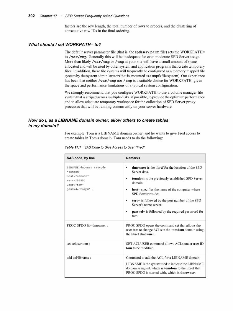
factors are the row length, the total number of rows to process, and the clustering ofconsecutive row IDs in the final ordering.

What should I set WORKPATH= to?The default server parameter file (that is, the spdsserv.parm file) sets the WORKPATH=to /var/tmp. Generally this will be inadequate for even moderate SPD Server usage.More than likely /var/tmp or /tmp at your site will have a small amount of spaceallocated and will be used by other system and application programs that create temporaryfiles. In addition, these file systems will frequently be configured as a memory mapped filesystem by the system administrator (that is, mounted as a tmpfs file system). Our experiencehas been that neither /var/tmp nor /tmp is a suitable choice for WORKPATH, giventhe space and performance limitations of a typical system configuration.

We strongly recommend that you configure WORKPATH to use a volume manager filesystem that is striped across multiple disks, if possible, to provide the optimum performanceand to allow adequate temporary workspace for the collection of SPD Server proxyprocesses that will be running concurrently on your server hardware.

How do I, as a LIBNAME domain owner, allow others to create tablesin my domain?

For example, Tom is a LIBNAME domain owner, and he wants to give Fred access tocreate tables in Tom's domain. Tom needs to do the following:

Table 17.1 SAS Code to Give Access to User "Fred"

SAS code, by line Remarks

LIBNAME dmowner sasspds"tomdom"host="samson"serv="5555"user="tom"passwd="tompw" ;

• dmowner is the libref for the location of the SPDServer data.

• tomdom is the previously established SPD Serverdomain.

• host= specifies the name of the computer whereSPD Server resides.

• serv= is followed by the port number of the SPDServer's name server.

• passwd= is followed by the required password fortom.

PROC SPDO lib=dmowner ; PROC SPDO opens the command set that allows theuser tom to change ACLs in the tomdom domain usingthe libref dmowner.

set acluser tom ; SET ACLUSER command allows ACLs under user IDtom to be modified.

add acl/libname ; Command to add the ACL for a LIBNAME domain.

LIBNAME is the syntax used to indicate the LIBNAMEdomain assigned, which is tomdom to the libref thatPROC SPDO is started with, which is dmowner.


SAS code, by line Remarks

modify acl/LIBNAME fred=(Y,Y,,) ; Modifies the ACL in the LIBNAME domain ACL togive user ID fred read and write access to thetomdom domain.

quit ;

Fred can now connect to the TOMDOM domain and create tables.

How does the system administrator list the access control lists for"user 1"?

To see the ACL privileges for a domain, the system administrator lists them for each user.

For this to work, your SPD Server user ID must be previously set up to have the SPECIAL(level 7) privilege, to use the ACLSPECIAL=YES option on a LIBNAME statement.

Table 17.2 Code to List ACLs

Command from command prompt > Remark

LIBNAME test saspds

'temp'

server=servname.7880

prompt=yes ;

Issue LIBNAME statement for testdomain, specify server and portnumber, ask system for a passwordprompt.

user="username" aclspecial=YES ; aclspecial=YES now gives"username" access to special ACLcommands, such as setting a new userID.

PROC SPDO lib=test ; Connects to the temp LIBNAMEdomain using the libref test.

set acluser user1 ; Sets the SPD Server user scope touser1.

list acl _all_ ; Lists all ACLs owned by user1.

The resulting output, described in the table below, lists all of the tables in "test".

Table 17.3 Results from List Command

Resulting output from list acl _all_; command Remarks

The SAS System 10:58 Tuesday, November 17, 2003 System message

ACL Info for A.DATA This ACL will affect table A if table A exists and user1is the owner or has ACL control of the table A.

Owner = USER1 USER1 created and owns the A.DATA ACL.

How does the system administrator list the access control lists for "user 1"? 303

Resulting output from list acl _all_; command Remarks

Group = TECH This ACL was created while user1was connected withan ACL group of TECH. All group permissions willaffect the permissions of the members of the TECHACL group.

Default Access (R,W,A,C) = (Y,N,N,N) R=Read; W=Write; A=Alter (rename, delete, or replacetables) C=Control (define and update ACLs for a table)

Y=Yes; N=No;

Universal privileges are limited to read on tableA.DATA.

Group Access (R,W,A,C) = (N,N,N,N) Users in the ACL group TECH have no privileges ontable A.DATA.

The SAS System 10:58 Tuesday, November 17, 2003

ACL Info for NTE*.DATA NTE*.DATA refers to a set of tables, which begin withNTE. ACLs of this kind are created using the genericoption. If you create a specific ACL for a table that startswith NTE, the specific ACL will override the genericACL.

Owner = user1

Group = TECH

Default Access (R,W,A,C) = (N,N,N,N)

Group Access (R,W,A,C) = (Y,Y,N,N) Users from the ACL group TECH have read and writeaccess to tables with names that start with NTE.

How do I change existing PROC SQL code that works with SAS toquery SPD Server tables?

OverviewYou do not have to change your PROC SQL code. The way to do this is to wrap your codeinside a CONNECT statement, which points to the location of the SPD Server tables. Thistechnique is referred to as pass-through. Normal operating system and ACL privilegesapply to the user ID making the query during the CONNECT process. Your PROC SQLcode should work with a few exceptions. For more information, see “Differences betweenSAS SQL and SPD Server SQL ” on page 141. .

Once you establish a working CONNECT statement which points to the location of yourSPD Server tables, you can assign a LIBNAME to the SPD Server table path with a librefcommand. This allows the simple name you assign to the SPD Server table to be used inthe SQL query, which keeps your SQL query as short as possible.

Here are four progressive examples:

• “Example 1: PROC SQL query, designed to work with a SAS data set, with a two-levelSAS filename example.” on page 305 shows PROC SQL that works with SAS.


• “Example 2: PROC SQL query, without using pass-through, pointing to an SPD Servertable, with a two-level SAS filename.” on page 305 shows how you can access SPDServer tables without using the Pass-Through Facility.

• “Example 3: PROC SQL query, using pass-through, pointing to an SPD Server table,with a LIBNAME example, with SQL code modified, to avoid using a two-level SASfilename.” on page 306 shows how you can access the SPD Server tables by changingyour PROC SQL code.

• “Example 4: PROC SQL query, using pass-through, pointing to an SPD Server table,executing a libref statement on the server, so that existing code can be used "as is".”on page 307 shows how you can use the original PROC SQL code from the firstexample, wrapped with a CONNECT statement, so that it can query SPD Server tables.

Example 1: PROC SQL query, designed to work with a SAS data set,with a two-level SAS filename example.

Table 17.4 Example 1 Code

Code Remarks

/* Issue a LIBNAME statement which */ /* creates a LIBREF called "test" */ LIBNAME test '/path/for/your/data' ; /* Query using base LIBREF of test */ PROC SQL ; select sum(table1+table2) as pass, carrier from test.carriers where carrier in('AA','JI') and bstate='TX' group by carrier ; quit ;

This is an example of SQL code that works with SAS.The code contains a two-level SAS filename reference,which is typical for PROC SQL, but it will not work ifwe attempt to use it inside of a pass-through CONNECTstatement.

Each of the following examples will show variations ofthis code, modified to access SPD Server information.We'll also discuss the pros and cons of each method.

Example 2: PROC SQL query, without using pass-through, pointingto an SPD Server table, with a two-level SAS filename.Why would you want to do this? You might NOT want to do this, because without pass-through, all the processing is done on the CPU of the client machine. When processinglarge tables, this is impractical, if not impossible.

How do I change existing PROC SQL code that works with SAS to query SPD Server tables?305


Code Remarks:

/* Issue a SPD Server (mkt) library *//* LIBNAME statement */

LIBNAME mkt sasspds 'mkt' server=servername.4228 user='anonymous' ; PROC CONTENTS data=mkt.carriers ; run ;/* query spds LIBREF (mkt) *//* (two-level SAS file name) */ PROC SQL; select sum(table1+table2) as pass, carrier from mkt.carriers where carrier in ('AA','JI') and bstate='TX' group by carrier ; quit ;

This example shows you how to make a query againstSPD Server tables, using your original SQL code,without using SQL pass-through.

Example 3: PROC SQL query, using pass-through, pointing to an SPDServer table, with a LIBNAME example, with SQL code modified, toavoid using a two-level SAS filename.Why would you want to do this? By modifying your SQL code slightly, you can use thePass-Through Facility to have SPD Server perform the work and send the results to theclient.


Code

//* Query spds LIBREF (mkt) (pass-through one-level LIBREF )*/ PROC SQL; connect to sasspds (dbq='mkt' serv='8770' user='anonymous' host='localhost') ; select * from connection to sasspds

(select sum(table1+table2) as pass, carrier from carriers where carrier in('AA','JI') and bstate='TX' group by carrier) ; quit ;


Example 4: PROC SQL query, using pass-through, pointing to an SPDServer table, executing a libref statement on the server, so thatexisting code can be used "as is".Why would you want to do this? Without modifying your SQL code, you can use thePass-Through Facility so SPD Server performs the work and sends the results to the client.


Code

PROC SQL ; connect to sasspds (dbq='mkt' serv='8770' user='anonymous' host='localhost'); /* Issue passthru LIBREF (mkt) for use */ /* in two-level queries */ execute(LIBREF mkt) by sasspds; /* Query the SPD Server LIBREF (mkt) */ /* that is a pass-through LIBREF */ select * from connection to sasspds

(select sum(table1+table2) as pass, carrier from mkt.carriers where carrier in('AA','JI') and bstate='TX' group by carrier) ; quit;

Can I use pass-through async to create multiple indexes on a singleexisting table?

No. Multiple create indexes on the same existing table are not supported with async.

PROC DATASETS can be used to create indexes in parallel for a single existing table.

For example:

PROC DATASETS lib=foo ;modify customer( asyncindex=yes bitindex=(state) ;index create state ;index create phoneno ;index create custno ;index create totsales ;quit ;

Can I use pass-through async to create multiple indexes on a single existing table? 307

Can I use pass-through async to create multiple indexes on existingtables?

Yes. As long as you create only one index per table, the index creation can be run withasync.

For example, to create an index State on table Customer, an index Totals on table Billing,and an index Orderno on table Orders asynchronously, you use the following code:

execute(begin async operation) by sasspds ;

execute(create index state on customer(state)) by sasspds ;

execute(create index totals on billing(totals)) by sasspds ;

execute(create index orderno on orders(orderno)) by sasspds ;

execute(end async operation) by sasspds ;

What size increases can I expect for tables that are stored in domainswith BACKUP=YES?

Tables created in domains that have Backup=YES will have an additional 17 bytes perobservation.


Your Turn

We welcome your feedback.

• If you have comments about this book, please send them to [email protected]. Include the full title and page numbers (if applicable).

• If you have comments about the software, please send them to [email protected].

SAS® Publishing Delivers!Whether you are new to the work force or an experienced professional, you need to distinguish yourself in this rapidly changing and competitive job market. SAS® Publishing provides you with a wide range of resources to help you set yourself apart. Visit us online at support.sas.com/bookstore.

SAS® Press Need to learn the basics? Struggling with a programming problem? You’ll find the expert answers that you need in example-rich books from SAS Press. Written by experienced SAS professionals from around the world, SAS Press books deliver real-world insights on a broad range of topics for all skill levels.

s u p p o r t . s a s . c o m / s a s p r e s sSAS® Documentation To successfully implement applications using SAS software, companies in every industry and on every continent all turn to the one source for accurate, timely, and reliable information: SAS documentation. We currently produce the following types of reference documentation to improve your work experience:

• Onlinehelpthatisbuiltintothesoftware.• Tutorialsthatareintegratedintotheproduct.• ReferencedocumentationdeliveredinHTMLandPDF– free on the Web. • Hard-copybooks.

s u p p o r t . s a s . c o m / p u b l i s h i n gSAS® Publishing News Subscribe to SAS Publishing News to receive up-to-date information about all new SAS titles, author podcasts, and new Web site features via e-mail. Complete instructions on how to subscribe, as well as access to past issues, are available at our Web site.

s u p p o r t . s a s . c o m / s p n

SAS and all other SAS Institute Inc. product or service names are registered trademarks or trademarks of SAS Institute Inc. in the USA and other countries. ® indicates USA registration. Otherbrandandproductnamesaretrademarksoftheirrespectivecompanies.©2009SASInstituteInc.Allrightsreserved.518177_1US.0109

sas scalable performance data (spd) server 4.5: user's guide

Documents