- 1 -

SAS®

Workshop

Manitoba Centre for Health Policy

University of Manitoba

Input and Development by:

Charles Burchill, Heather Prior, Wendy Au, Jen Bodnarchuk, Randy Walld

Shelley Derksen, Jill MacGregor, Ruth-Ann Soodeen, and Ruth Bond

September 2017

- 2 -

- 3 -

Table of Contents Outline ................................................................................................................................................................................................................................. 5

Textbook ....................................................................................................................................................................................................................... 6 CD Content ................................................................................................................................................................................................................... 6 Getting SAS (UofM Students and Staff only) ................................................................................................................................................................ 6

Data Use Agreement ............................................................................................................................................................................................................ 7 Overview ............................................................................................................................................................................................................................. 9

Why Programming? ...................................................................................................................................................................................................... 9 SAS Dataset Structure ................................................................................................................................................................................................... 9 Programming Structure ............................................................................................................................................................................................... 10

SAS Display Manager Interface ......................................................................................................................................................................................... 11 Structured SAS Code Suggestions. .................................................................................................................................................................................... 13

General suggestions. ................................................................................................................................................................................................... 13 Data step ..................................................................................................................................................................................................................... 13 Macro code ................................................................................................................................................................................................................. 15 Procedures ................................................................................................................................................................................................................... 15 Comments ................................................................................................................................................................................................................... 15 Test code ..................................................................................................................................................................................................................... 15

SAS Programming Examples ............................................................................................................................................................................................. 17 Example 1 ................................................................................................................................................................................................................... 17

* Part I: Viewing Data ; .......................................................................................................................................................................... 17 * Part II: Exploring the data; ............................................................................................................................................................. 19

Example 2 ................................................................................................................................................................................................................... 21 * Part I: Import Data, Use of Formats and Labels ; .................................................................................................................. 21 * Part II: Sub-setting & Manipulating data, & Creating Variables; .................................................................................. 24 * Part III: Getting Data Out of SAS through PROC EXPORT and ODS ; ................................................................................ 27

Example 3 ................................................................................................................................................................................................................... 29 * Part I: SAS Options (printing); ....................................................................................................................................................... 29 * Part II: Sorting Data with Proc Sort; .......................................................................................................................................... 29 * Part III: Setting or Concatenation of Data ; ........................................................................................................................... 30 * Part IV. Merging or adding variables; .......................................................................................................................................... 31 * Part V: Use of Put() with formats for creating variables; ............................................................................................... 33 * Part VI: Type Conversions put/input ; .......................................................................................................................................... 35

Example 4 ................................................................................................................................................................................................................... 38 * Part I: By group processing for Longitudinal Data ; ............................................................................................................ 38 * Part II. Groups of Variables & Array processing; .................................................................................................................. 41

* SESSION 5. ; ........................................................................................................................................................................................................... 44 * Part I: Date time processing ; ......................................................................................................................................................... 44 * Part II: SQL Processing ; ................................................................................................................................................................... 46

Graphic User Interface to SAS (point-and-click) ............................................................................................................................................................... 52 SAS Explorer and ViewTable using the SAS Display Manager .................................................................................................................................. 52 SAS IML Studio.......................................................................................................................................................................................................... 55 SAS Enterprise Guide ................................................................................................................................................................................................. 56

Enterprise Guide Environment ............................................................................................................................................................................. 56 Define SAS Library .............................................................................................................................................................................................. 58 Loading SAS Data ................................................................................................................................................................................................ 59 Data Manipulation – sort, merge, concatenation, formats ..................................................................................................................................... 60 Analysis, Options, and SAS code ......................................................................................................................................................................... 61 Task Output .......................................................................................................................................................................................................... 63 Using your Own Code .......................................................................................................................................................................................... 64 Running a Process Later ....................................................................................................................................................................................... 68

Practice Questions ............................................................................................................................................................................................................. 69 SAS Workshop Practice Questions #1 ......................................................................................................................................................................... 69 SAS Workshop Practice Questions #2 ......................................................................................................................................................................... 70 SAS Workshop Practice Questions #3 ......................................................................................................................................................................... 72 SAS Workshop Practice Questions #4 ......................................................................................................................................................................... 73 SAS Workshop Practice Questions #5 ......................................................................................................................................................................... 75

Data Dictionaries ............................................................................................................................................................................................................... 77 MCHP Training and Research Resource ........................................................................................................................................................................... 77

Height/Weight Dictionary ........................................................................................................................................................................................... 77 Hospital Dictionary ..................................................................................................................................................................................................... 77

CCI Rubric Formats ............................................................................................................................................................................................. 79 Physician Medical Services Dictionary ....................................................................................................................................................................... 86 Tariff Dictionary ......................................................................................................................................................................................................... 93 Registry Dictionary ..................................................................................................................................................................................................... 95 Family Registry Dictionary ......................................................................................................................................................................................... 97 Census Dictionary ....................................................................................................................................................................................................... 98 Prescription Drug Dictionary..................................................................................................................................................................................... 104 ATC Codes Dictionary .............................................................................................................................................................................................. 107 Drug Cost Dictionary ................................................................................................................................................................................................ 108 Provided SAS Macro Code ....................................................................................................................................................................................... 109

Common SAS Statements, Functions, Formats, & Procedures ......................................................................................................................................... 111

- 4 -

- 5 -

Outline

The MCHP SAS workshop will provide the necessary SAS programming skills to work

with SAS and administrative data. The workshop unfortunately cannot provide an

introduction to a wide variety of statistical analyses. It will provide an understanding of

how to use SAS statistical procedures and how to find the necessary statements and

options to use the procedures. The SAS programming language is stressed in this course

instead of interactive analysis for a number of reasons: a) replications of results, b)

efficiency of programming, c) access to 'advanced' options, d) helping fulfill the

requirements for documentation of research outlined in UofM Policy on Responsibilities

for Research Ethics.

The workshop is broken down into five half day sessions with examples and problems to

work through. The workshop was setup to complete with an instructor as not all of the

code is fully documented.

Session 1: Using basic SAS procedures and understanding PROC syntax

I. Viewing data

II. Exploring data.

Session 2: Creating and Manipulating Data

I. Import of data into SAS

Use of formats to modify displayed data

II. Manipulating data

Use of logical if/then/else statements

Creating new variables.

III. Getting Data out of SAS

Session 3: Combining Datasets

I. SAS Options (printing)

II. Sorting of data

III. Setting or concatenation of data

IV. Merging or adding variables using a 'by' statement.

V. Use of Put() with formats for creating variables

VI. Type conversions put/input

Session 4: Longitudinal and Cross sectional Processing

I. By group processing for longitudinal data (first, last, retain).

II. Variable Groups & Array processing for cross sectional data.

Session 5: Date processing, SQL, and Interactive SAS;

I. Date time processing

II. SQL

III. Interactive SAS, SAS Enterprise Guide

- 6 -

IV. Finish up anything not covered earlier

Textbook

Delwiche, Lora D., and Slaughter, Susan J. 'The Little SAS Book: A Primer, 5th edition,

2012.

This book is recommended for anyone working with SAS. It provides a basic overview of the SAS

language with practical examples - it covers more material than is covered in the MCHP workshops. It does

not provide much direction or help with statistical procedures or analysis. Although we do not follow the

order of information presented in the book the text throughout this course provides further reading and

references. Specific reading material is identified with LSB (Little SAS Book) followed by a section

number and page range.

Starting in 2014 SAS is offering SAS University Edition. This is a freely available

interface to SAS (including Base SAS and SAS/STAT) that will run on most computer

operating systems (including the Mac). More information and downloads can be found

from SAS (http://blogs.sas.com/content/sastraining/2014/06/18/free-sas-software-for-

students/).

Downloads and installation: http://www.sas.com/en_us/software/university-

edition/download-software.html

The minimum requirements are: 64bit Windows 7, minimum 1GB RAM, ~2GB disk; OS

X 10.8, minimum 1GB ram, ~2GB disk space.

SAS Online Documentation

http://support.sas.com/documentation/

Google suggestion for further help When using Google to search for material start your search string with ‘SAS’, ‘PROC’ or both. Adding

SGF or SUGI will usually identify papers from the SAS international conferences – these are reviewed and

typically well written with good examples.

CD Content A CD or DVD should be provided with this material that contains all of the data, programs (including

log/list files) and supporting documentation that is used in this workshop.

Getting SAS (UofM Students and Staff only)

If you need to license a copy of SAS for your own computer please contact the UofM ACN support desk

(474-8600, support@cc.umanitoba.ca) to make arrangements. The annual license copy (2016) was $100.00.

You can find license information on the WWW at:

http://umanitoba.ca/computing/ist/software/licensed.html

Look under SAS and click on the link 'home/campus use' to get the forms to fill out.

You will need the Standard Install package - you might be able to work with your peers to get only one

copy of the media. You might need to contact the ACN Support Desk at the Fort Garry campus (010 Dafoe

Tunnel) at 474-8600, or by E-mail at support@cc.umanitoba.ca for distribution details.

SAS® and all other SAS Institute Inc. product or service names are registered trademarks or trademarks of

SAS Institute Inc. in the USA and other countries. ® indicates USA registration.

- 7 -

MCHP SAS Workshop

Data Use Agreement The Manitoba Health, Healthy Living and Seniors (MH) monitors use of medical administrative data

through the Health Information Privacy Committee (HIPC). The importance of the Manitoba Health data

repository has been recognised in an agreement reached between the University of Manitoba and MH. The

University has accepted responsibility for assuring confidentiality of these data. Any effort to determine the

identity of any reported cases, or to use the information for any purpose other than for health statistical

reporting and analysis, would be against the law. MH and the University do everything possible to assure

that the identity of data subjects cannot be disclosed through public-use data sets; all direct identifiers, as

well as any characteristics that might lead to identification are omitted from the data set. Nevertheless, it

may be possible in rare instances, through complex analysis and with outside information on sample cases,

to ascertain from the data set the identity of particular persons or establishments. Considerable harm could

ensue if this were done.

The data provided for the MCHP SAS workshop, have been simulated to resemble data from MH, and are

provided for educational purposes only. They contain no information that would allow identification of

individuals or physicians except as described in the preceding paragraph.

The undersigned gives the following assurances with respect to use of simulated data for the SAS

workshop:

- The data in these sets will not be used in any way except for statistical reporting and analysis;

- The data sets or any part of them will not be released to any other person;

- The data sets will not be used in a manner to learn the identity of any person or establishment included

in any set;

- If the identity of any person or establishment should be discovered inadvertently, then (a) no use will

be made of this knowledge, (b) the course instructors will be advised of the incident, (c) the

information that would identify an individual or establishment will be safe-guarded or destroyed, as

requested by the course instructors, and (d) no one else will be informed of the discovered identity; and

- After completion of the course, the original data will be returned to the course instructors and all newly

created data sets will be destroyed.

Signed:

Name (printed):

Address or Contact:

Date:

- 8 -

Page intentionally left blank

- 9 -

Overview The following overview based on the introductory PowerPoint presentation for the

workshop it does not contain all of the information covered in the presentation.

Why Programming?

Programming, rather than ‘Point-and-Click’ interface, provides the ability to quickly

replicate results once code is written, provides some efficiency through the ability to copy

and ‘tweak’ existing code. Programming saves time by not having to step through an

iterative process every time a new analysis is required. Use of code provides access to

advanced options and capabilities. Finally, if nothing else, it helps meet the requirements

outlined in UofM Research Policy (1406). Although this workshop is primarily focused

on programming in SAS an introduction to SAS IML Studio and SAS Enterprise Guide

has been included. These two applications provide a graphic user interface to many SAS

procedures and data manipulation tools.

SAS Dataset Structure

SAS definition of a SAS Data Set (LSB s1.2 pp4-5, s1.11 pp22-23, s2.19 pp66-67): A

SAS data set consists of data values and their associated descriptive information

organized in a rectangular form that can be recognized by the SAS System. SAS data sets

always contain the following two components:

1) Data values that are organized into variables (columns) and observations

(rows)

VARIABLES

OB

SE

RV

AT

ION

S

Values

- 10 -

2) Descriptor information that identifies the attributes of both the data set and its

data values.

The columns, or data elements, are called variables in SAS data sets. The rows, or

records, are called observations. Each observation is a collection of values for the

variables.

Programming Structure

The Base SAS programming language is an interpreted language that is written as ASCII

text and 'submitted' to SAS to compile and run. The program is written as a set of

statements. Statements typically start with a keyword and end with a semicolon. Most

statements are grouped into steps (LSB s1.3 pp6-7). SAS also comes with several other

related languages (SAS Macro, Screen Control, Template, and Interactive Matrix). It is

possible to compile SAS statements into stored code for general use but that process is

outside the scope of this workshop.

When first writing and debugging a SAS program it is best to use a structure that is easy

to read, run the programs in small sections, and test with small datasets (obs=__ option).

If possible, use a syntax sensitive editor (e.g. SAS editor) that colourizes your text

depending on the context.

SAS Statements (Basic Building Block)

– Start with key word, and end with semi colon

– Typically a there is one statement/line

bmi = (weight/2.2)/(height*0.0254)**2;

Statements are grouped into Steps for analytic and data management.

– Start with PROC or DATA statement & end with RUN;

– PROC steps are used to do analyses or view data

– DATA steps are used to manipulate Data

proc print data=htwt ;

var name sex age height weight ;

run;

data test ;

set test ;

bmi = (weight/2.2)/(height*0.0254)**2;

run;

{

{

- 11 -

SAS Display Manager Interface

When you first run SAS a display with multiple screens appears by default. These screens

are the place where you interact with SAS; you tell it what to do and where results are

displayed.

There are three primary windows.

1. Enhanced Program Editor.

a. This is a basic text editor and is really the only place (for this session) that

you will input commands and interact with SAS.

b. Colorized words

i. Green comments

ii. Dark blue SAS statements and step boundaries

iii. Blue statements and key words

iv. Purple quoted text

c. Programs can be run as a whole or in parts.

i. Select portion that you want to run click the running man.

ii. Alternatively F3 or F8 can be used from the key board.

d. The program editor is where you would save and recall your programs.

2. Log Window

a. This displays how SAS has interpreted your request (or program)

b. The log should always be reviewed for warnings and errors prior to

looking at any results.

c. Colorized sections

i. Black is your original code

ii. Blue text is information notes. Generally notes mean that things

have run OK but always check to see that there is a note after a

data step or procedure and that the numbers of records (and

sometimes variables) makes sense. Look for notes containing

uninitialized variables, character or numeric conversions, and

iii. Green text is warnings that should be resolved. These generally

will not stop SAS from running but might reset some options and

usually will cause data problems.

iv. Red text identifies errors that must be resolved.

d. The log file continues to grow as you run portions of your SAS program.

3. Output Windows

a. The output window contains the resulting output (generally statistical

results) that has been generated by any SAS procedures.

b. The output window continues to grow as you run portions of your SAS

program.

You can move between these primary windows by clicking on the log/output/program

buttons on the bottom task bar.

- 12 -

When you are working in SAS it is generally a good idea to save your program, log, and

output (list). This way you can review the results and log at a later point in time.

A good practice is to write and test small portions of your then clear the log/output

windows and run the whole program once to make sure that your log and output are all

consistent and are using the data that you expect/want. Try to enter separate SAS

statements on each line with comments to describe what is being done.

There are two other secondary windows that allow you to explore the SAS environment

and results. These are found on the left side of the main SAS Windows.

1. The explorer window will allow you to open SAS datasets, get information on

SAS datasets, copy and delete SAS datasets. When you open A SAS dataset from

the explore window you can see the value it contains.

2. The results window allows you to quickly access all of the results in your output

window.

More recent versions of SAS may start the SAS Enterprise Guide interface by default.

Getting Things Started

1. PROGRAM EDITOR

2. LOG OF SAS JOB

3. OUTPUT WINDOW

RUN SELECTION

EXPLORE

DATA &

RESULTS

- 13 -

Structured SAS Code Suggestions. The following are some suggestions for SAS programming structure. Some alternatives

have also been mentioned.

General suggestions.

1. Maintain one case (upper or lower) mixing cases with out reason makes code

difficult to read. As a side note: on systems that allow upper and lower case

most programmers use lower case - it is generally easier to read.

2. Every program should have an introductory comment.

/******

File name: Date:

Author:

Description:

Study:

If applicable the following should also be added.

Principal Investigator:

Input Data:

Output Data:

Variables Generated:

External files:

*******/

3. The introductory comment may be enclosed in a box.

4. If multiple programs have been used to generate some result a file titled

README.txt or readme.txt should be included in the directory with the

purpose and order of each program.

5. SAS program files should end with .sas, list files with .lst, and log files with

.log.

6. Code so you and others can understand your code.

Remember Occam's Razor. (After William of Ockham (1300-1349? English

philosopher) a philosophical or scientific principle according to which the best

explanation of an event is the one that is the simplest, using the fewest

assumptions, hypotheses, etc...)

7. If possible all libraries, %include files, formats, macros and other general code

should go at the top of the program, or be referenced in the initial comment.

8. Data set names should reflect the contents of the data set. A data set label

should be added to any permanent SAS data sets.

9. Try to keep individual lines shorter than 80 characters.

Data step

1. Data statement should be left justified. If options carry over then line up with

initial brackets or indented 8 spaces.

- 14 -

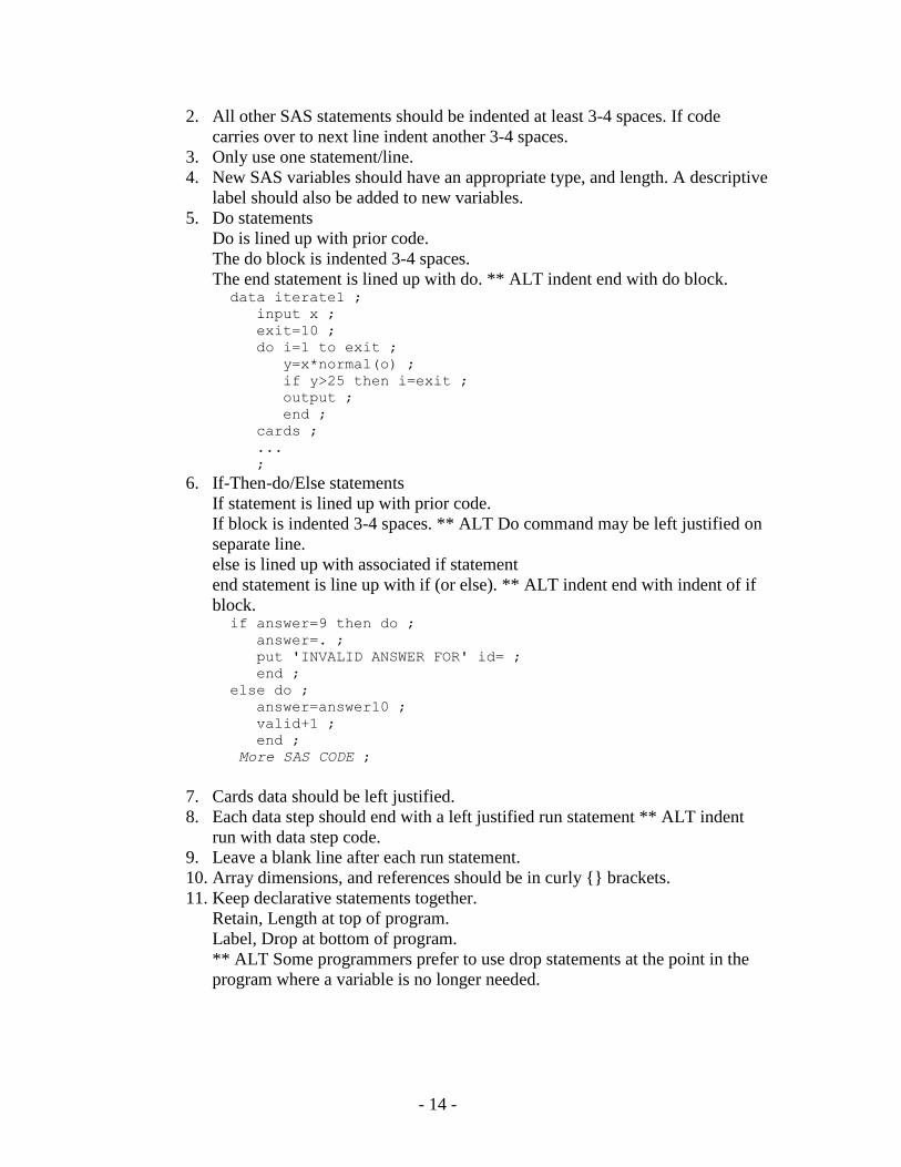
2. All other SAS statements should be indented at least 3-4 spaces. If code

carries over to next line indent another 3-4 spaces.

3. Only use one statement/line.

4. New SAS variables should have an appropriate type, and length. A descriptive

label should also be added to new variables.

5. Do statements

Do is lined up with prior code.

The do block is indented 3-4 spaces.

The end statement is lined up with do. ** ALT indent end with do block. data iterate1 ;

input x ;

exit=10 ;

do i=1 to exit ;

y=x*normal(o) ;

if y>25 then i=exit ;

output ;

end ;

cards ;

...

;

6. If-Then-do/Else statements

If statement is lined up with prior code.

If block is indented 3-4 spaces. ** ALT Do command may be left justified on

separate line.

else is lined up with associated if statement

end statement is line up with if (or else). ** ALT indent end with indent of if

block. if answer=9 then do ;

answer=. ;

put 'INVALID ANSWER FOR' id= ;

end ;

else do ;

answer=answer10 ;

valid+1 ;

end ;

More SAS CODE ;

7. Cards data should be left justified.

8. Each data step should end with a left justified run statement ** ALT indent

run with data step code.

9. Leave a blank line after each run statement.

10. Array dimensions, and references should be in curly {} brackets.

11. Keep declarative statements together.

Retain, Length at top of program.

Label, Drop at bottom of program.

** ALT Some programmers prefer to use drop statements at the point in the

program where a variable is no longer needed.

- 15 -

Macro code

1. Follows same indenting rules as data step code.

2. All internal code should be indented after the %macro statement.

3. Clearly comment all your macro code, and variables.

o %* comments will not show up in the resolved macro code

o * comments will appear in resolved code

4. Macros should not be defined, and compiled from within a macro.

Procedures

1. Proc statement should be left justified. If options carry over to the next line they

should be indented 8 spaces.

2. Use only one statement/line.

3. Indent procedure statements 3-4 spaces. If the statement is longer than one line

then each subsequent line should be indented at least 8 spaces.

4. Each procedure should end with a run, and or quit statement.

5. Leave a blank line after each run statement.

proc format data=jumbo.data ;

where slice='1' ;

tables a*b c*d / noprint out=temp ;

run;

proc chart data=interm.grades ;

block section / midpoints='Mon' 'Wed' 'Fri'

group=sex

sumvar=grade type=mean ;

title 'Comparing the Mean for GRADE among Sections' ;

run;

Comments

1. Justify to the code that is being commented.

2. Use ** ; type comments within code, or data statements This will allow /**

**/ to be used to block out and run test sections.

3. Comments apply to next line or block of code.

Test code

If you want to add test code to your program such as put _all_ ; it should be left

justified. This will make it much easier to see and remove the code later ;

- 16 -

Page intentionally left blank

- 17 -

SAS Programming Examples

Example 1 * f=htwt_example1.sas * * * * Part I Viewing the data using PROC CONTENTS * * and PROC PRINT * * Part II Exploring the data using PROC FREQ * * and PROC MEANS and other procedures * ******************************************; * Introduction to workshop * SAS Program and Language (LSB s1.1 pp2-3, s1.3 pp6-7). The SAS programming language is an interpreted language that is written as ASCII text and 'submitted' to compile and run. The program is written as a set of statements. Statements typically start with a keyword and end with a semicolon. Most statements are grouped into steps (LSB s1.3 pp6-7) ; * Writing SAS programs that work (LSB s11.1 pp296-297). When writing a SAS program it is best to use a structure that is easy to read. Run the programs in small sections, possibly with small datasets. If possible, use a syntax sensitive editor (e.g. SAS editor) that colourizes your text depending on the context. Review log messages after each step and resolve any errors, warnings or notes. After basic syntax problems, the most common mistakes are caused by missing semi-colons and unclosed quotes. * Introduction to SAS Procedures (LSB s1.3 6-7, s2.21 pp70-71, s4.1 pp100-101): 1) Proc Contents - provides a description of the contents of a SAS data set 2) Proc Print - provides a print out of a SAS data set 3) Proc Freq - provides frequency distributions of variables 4) Proc Means - provides descriptive statistics of variables; * SAS procedures are used to analyze data. They are always invoked with the SAS keyword, PROC, followed by the name of the procedure.; *SAS definition of a SAS Data Set (LSB s1.2 pp4-5, s1.10 pp20-21, s2.18, s2.19 pp64-67). A SAS data set consists of data values and their associated descriptive information organized in a rectangular form that can be recognized by the SAS System. SAS data sets always contain the following two components: 1)data values that are organized into columns and rows 2)descriptor information that identifies the attributes of both the data set and its data values. The columns, or data elements, are called variables in SAS data sets. The rows, or records, are called observations. Each observation is a collection of values for the variables.; * SAS data sets can be permanent or temporary (LSB s2.18 pp64-65). Permanent SAS data sets are permanently stored in a SAS library. Temporary SAS data sets are created within a SAS session and are available throughout the SAS session. They are destroyed when the SAS session is over.; * This program uses a permanent SAS data set called HTWT. It is stored on your computer in a folder called X:\course.;

* Part I: Viewing Data ; * To access a permanent SAS data set, you must specify a library reference to the folder/path where the data are stored (external storage location);

- 18 -

* Use the libname statement to describe the path where the permanent SAS data sets are stored (LSB s2.19 pp66-67); libname course 'X:\course\data'; * Use title and footnote statements to give your output titles and footnotes (LSB s4.1 p100-101). These can be used with all procedures that produce output.; title 'Data= Course.HTWT'; footnote 'SAS Workshop'; * Proc contents describes what is in a SAS dataset, i.e. its contents (LSB s2.21 pp70-71). The 'data=' procedure option identifies the SAS dataset that you want to use.; title 'Proc Contents of Course.htwt'; proc contents data=course.htwt ; run; *If you want to know about all of the datasets in a library, use the keyword _all_. Proc contents has many such options. Use the online help or SAS reference manuals to find out more options; title 'Proc Contents of Course._all_'; proc contents data=course._all_ ; run; * Proc print prints out SAS datasets to the output window (LSB s4.5 pp108-109). If you have a large dataset, use the dataset option obs= to limit the number of observations printed. SAS has many dataset options available. You can specify data set options in parentheses after the data set name. I was able to find a list of the data set options by going through SAS Help: - SAS System Help -> Index -> Data Set Options -> summary of (or by category) - SAS System Help -> Contents tab -> SAS Products -> Base SAS -> SAS Language Dictionary -> SAS Data Set Options - http://support.sas.com/documentation/cdl/en/lrdict/64316/HTML/default/viewer.htm#a002295655.htm - Base SAS, SAS Language Reference: Dictionary, Dictionary of Language Elements, SAS Data Set Options - Index tab - Jump to: data options -> press the next link at the bottom (LSB s6.1 pp178-179); title 'Proc Print with obs=10 Data Set Option'; proc print data=course.htwt(obs=10); run; * Use the proc print option noobs to suppress the observation number in the output. Proc Print has many options available. Each procedure has its own set of specific options and statements (s4 pp102-149). http://support.sas.com/documentation/cdl/en/proc/61895/HTML/default/viewer.htm#titlepage.htm - Base SAS, Base SAS Procedures Guide, Procedures - Index tab - Jump to: Print Procedure -> Proc Print statement ; title 'Proc Print with NOOBS option'; proc print data=course.htwt noobs; run; * Use the var statement within proc print to limit the variables printed; title 'Proc Print with VAR statement'; proc print data=course.htwt; var name sex age; run; * Use title and footnote statements to give your output titles and footnotes (LSB s4.1 p100-101). These can be used with all procedures that produce output.; title 'Data= Course.HTWT'; footnote 'SAS Workshop'; proc print data=course.htwt; run;

- 19 -

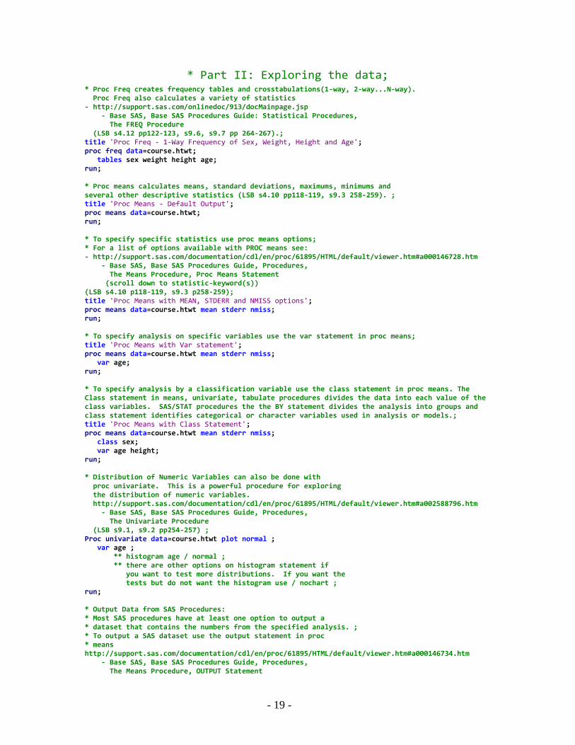
* Part II: Exploring the data; * Proc Freq creates frequency tables and crosstabulations(1-way, 2-way...N-way). Proc Freq also calculates a variety of statistics - http://support.sas.com/onlinedoc/913/docMainpage.jsp - Base SAS, Base SAS Procedures Guide: Statistical Procedures, The FREQ Procedure (LSB s4.12 pp122-123, s9.6, s9.7 pp 264-267).; title 'Proc Freq - 1-Way Frequency of Sex, Weight, Height and Age'; proc freq data=course.htwt; tables sex weight height age; run; * Proc means calculates means, standard deviations, maximums, minimums and several other descriptive statistics (LSB s4.10 pp118-119, s9.3 258-259). ; title 'Proc Means - Default Output'; proc means data=course.htwt; run; * To specify specific statistics use proc means options; * For a list of options available with PROC means see: - http://support.sas.com/documentation/cdl/en/proc/61895/HTML/default/viewer.htm#a000146728.htm - Base SAS, Base SAS Procedures Guide, Procedures, The Means Procedure, Proc Means Statement (scroll down to statistic-keyword(s)) (LSB s4.10 p118-119, s9.3 p258-259); title 'Proc Means with MEAN, STDERR and NMISS options'; proc means data=course.htwt mean stderr nmiss; run; * To specify analysis on specific variables use the var statement in proc means; title 'Proc Means with Var statement'; proc means data=course.htwt mean stderr nmiss; var age; run; * To specify analysis by a classification variable use the class statement in proc means. The Class statement in means, univariate, tabulate procedures divides the data into each value of the class variables. SAS/STAT procedures the the BY statement divides the analysis into groups and class statement identifies categorical or character variables used in analysis or models.; title 'Proc Means with Class Statement'; proc means data=course.htwt mean stderr nmiss; class sex; var age height; run; * Distribution of Numeric Variables can also be done with proc univariate. This is a powerful procedure for exploring the distribution of numeric variables. http://support.sas.com/documentation/cdl/en/proc/61895/HTML/default/viewer.htm#a002588796.htm - Base SAS, Base SAS Procedures Guide, Procedures, The Univariate Procedure (LSB s9.1, s9.2 pp254-257) ; Proc univariate data=course.htwt plot normal ; var age ; ** histogram age / normal ; ** there are other options on histogram statement if you want to test more distributions. If you want the tests but do not want the histogram use / nochart ; run; * Output Data from SAS Procedures: * Most SAS procedures have at least one option to output a * dataset that contains the numbers from the specified analysis. ; * To output a SAS dataset use the output statement in proc * means http://support.sas.com/documentation/cdl/en/proc/61895/HTML/default/viewer.htm#a000146734.htm - Base SAS, Base SAS Procedures Guide, Procedures, The Means Procedure, OUTPUT Statement

- 20 -

(LSB s4.11 p120-121); * The NOPRINT option suppresses the printed output generated * by proc means; proc means data=course.htwt noprint; class sex; var age height; ** summary statistics with variable names can be defined on the output statement. If variable names are not used the input variable names are used in the output. ; output out=summary mean=mean_age mean_height; run; proc print data=summary; title 'Dataset Output from Proc Means using the Output statement: Data=summary'; run; * The AUTONAME option causes the output variables to be called age_mean height_mean. If you have many summary statistics it shortens the lenght of the output statement. ; proc means data=course.htwt noprint; class sex; var age height; output out=summary mean= nmiss= /autoname; run; proc print data=summary; title 'Dataset Output from Proc Means using the Output statement & autoname: Data=summary'; run; * Simple regression (LSB s9.10 pp272-273) using PROC REG.

The REG procedure fits a linear regression using least-squares method.

There are other SAS procedures that will allow for different types of

regression and options (e.g. GLM, LOGISTIC, GENMOD) with a variety of distributions.

A variety of plots and output datasets can be created with various

options. If ODS graphics is available a wide range of additional

graphic output can be created;

proc reg data=course.htwt alpha=0.05 ;

model weight = height ;

output out=htwt_reg_out residual=resid predicted=pred l95m=lower u95m=upper ;

plot weight*height / pred ;

quit;

proc print data=htwt_reg_out ;

run;

** Proc glm (general linear model) can be used for a variety of linear models

including simple/multiple regression, ANOVA and others using the method

of least-squares to fit the model. String or categorical

Classification variables may be used. When using multiple independent variables

contrast statements can be used to compare individual levels within specific

variables. Contrast statements are found in a number of regression procedures;

proc glm data=course.htwt ;

class sex ;

model weight = height age sex / alpha=0.05 ;

contrast 'Compare Male vs Female' sex 1 -1 ;

output out=htwt_glm_out residual=resid predicted=pred lclm=lower uclm=upper ;

quit ;

proc print data=htwt_glm_out ;

run;

- 21 -

Example 2 * f=htwt_example2.sas * * * * Part I * Import data into SAS * Use of formats to label or group displayed data * * Part II * Create or use subsets of data Create new variables using if/then/else logic * Create new variables using SAS functions * Part III

Getting Data out of SAS ***********************************************************;

* Part I: Import Data, Use of Formats and Labels ; libname course 'X:\course\data'; * read htwt data into a temporary SAS dataset from in-line data using * a DATA STEP (LSB s2.4 pp36-37) Temporary data sets are stored in the WORK * library (LSB s2.18 pp64-65). The WORK library is automatically created at the * beginning of the SAS session. Temporary data sets are present in the * WORK library until the current SAS session is finished. The WORK library * and its contents are automatically deleted at the end of the session.; data htwt; /* Begin the DATA step */ /* Describe variable names and locations */ * Raw data is read using an INPUT statement; * Each line of data in the raw data file = 1 observation in the SAS dataset; * Each variable is read from the same column(s) in every line of data (LSB s2.6 pp40-41).; * This style of input is known as column input. SAS can read in several styles of input including (LSB s2.1-2.7 pp30-43): 1) List Input - Data values are not required to be aligned in columns but must be separated by at least one blank or other defined delimiter (such as a comma or a tab). 2) Formatted Input - Formatted input allows you to read in non-standard data such as numbers with commas embedded or unusual numeric formats such as packed decimal. 3) Named Input - really weird records where data values are preceded by the name of the variable and an equal sign.; * Each variable is assumed to be numeric unless you tell SAS it is character using $; input name $ 1-10 sex $ 12 age 14-15 height 17-18 weight 20-22; /* Read the following lines of raw data */ /*the key word CARDS can also be used */ datalines; Aubrey M 41 74 170 Ron M 42 68 166 Carl M 32 70 155 Antonio M 39 72 167 Deborah F 30 66 124 Jacqueline F 33 66 115 Helen F 26 64 121 David M 30 71 158 James M 53 72 175 Michael M 32 69 143 Ruth F 47 69 139 Joel M 34 72 163 Donna F 23 62 98 Roger M 36 75 160

- 22 -

Yao M . 70 145 Elizabeth F 31 67 135 Tim M 29 71 176 Susan F 28 65 131 ; /* End the lines of raw data */ run; /* End the DATA step */ /* Print the values of hte htwt dataset */ proc print data=htwt; /* Begin a PROC step */ title1 'Reading Raw Data into a SAS dataset'; title2 'HTWT Data'; run; /* End the PROC step */ * the label statement labels variables (LSB s4.1 p100-101); * add labels to variables in a SAS dataset; data htwt; set htwt; label name='First Name of Client'; label sex='Male/Female'; label age='Age of Client'; label height='Height in Inches'; label weight='Weight in Pounds'; run; proc contents data=htwt; title1 'Adding Variable Labels to a SAS Dataset'; run; * Use of formats to label or group displayed data ; * Formats can be used to label the values of variables (LSB s4.6 pp110-111); * You create formats to label values of variables using a SAS procedure called PROC FORMAT (LSB s4.8 pp114-115). Once formats are created, they are available for use in a Data Step or a Proc Step. Notice that you can group values into a single category in a format; Proc format; value $sexL 'M'='Male' 'F'='Female'; value agegrp 0-9 = '00-09' 10-19='10-19' 20-29='20-29' 30-39='30-39' 40-49='40-49' 50-59='50-59' 60-69='60-69' 70-high='70+'; run; * Once formats have been created (by the PROC FORMAT step), you can start to use them using a format statement.; * You can associate a format with a variable in a Data Step; * This will associate the format with a variable permanently; data htwt; set htwt; * The format statement associates the format ($SEXL) with a variable (SEX); * format sex $sexL.; ** run this code twice and uncomment the second time ; run; proc print data=htwt; title1 'Adding Value Labels to a SAS variable using FORMAT Statement'; run; * You can associate a format with a variable in a Proc Step; * This will associate the format with a variable temporarily ; Proc freq data=htwt; tables sex age; format age agegrp.;

- 23 -

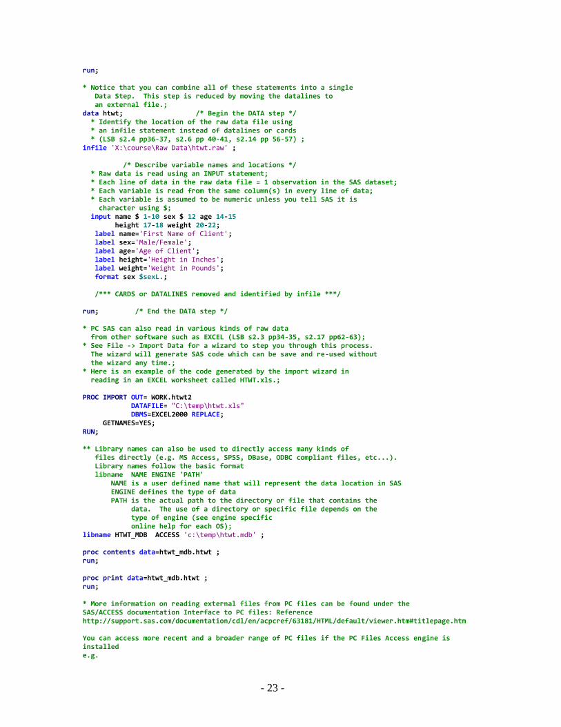
run; * Notice that you can combine all of these statements into a single Data Step. This step is reduced by moving the datalines to an external file.; data htwt; /* Begin the DATA step */ * Identify the location of the raw data file using * an infile statement instead of datalines or cards * (LSB s2.4 pp36-37, s2.6 pp 40-41, s2.14 pp 56-57) ; infile 'X:\course\Raw Data\htwt.raw' ; /* Describe variable names and locations */ * Raw data is read using an INPUT statement; * Each line of data in the raw data file = 1 observation in the SAS dataset; * Each variable is read from the same column(s) in every line of data; * Each variable is assumed to be numeric unless you tell SAS it is character using $; input name $ 1-10 sex $ 12 age 14-15 height 17-18 weight 20-22; label name='First Name of Client'; label sex='Male/Female'; label age='Age of Client'; label height='Height in Inches'; label weight='Weight in Pounds'; format sex $sexL.; /*** CARDS or DATALINES removed and identified by infile ***/ run; /* End the DATA step */ * PC SAS can also read in various kinds of raw data from other software such as EXCEL (LSB s2.3 pp34-35, s2.17 pp62-63); * See File -> Import Data for a wizard to step you through this process. The wizard will generate SAS code which can be save and re-used without the wizard any time.; * Here is an example of the code generated by the import wizard in reading in an EXCEL worksheet called HTWT.xls.; PROC IMPORT OUT= WORK.htwt2 DATAFILE= "C:\temp\htwt.xls" DBMS=EXCEL2000 REPLACE; GETNAMES=YES; RUN; ** Library names can also be used to directly access many kinds of files directly (e.g. MS Access, SPSS, DBase, ODBC compliant files, etc...). Library names follow the basic format libname NAME ENGINE 'PATH' NAME is a user defined name that will represent the data location in SAS ENGINE defines the type of data PATH is the actual path to the directory or file that contains the data. The use of a directory or specific file depends on the type of engine (see engine specific online help for each OS); libname HTWT_MDB ACCESS 'c:\temp\htwt.mdb' ; proc contents data=htwt_mdb.htwt ; run; proc print data=htwt_mdb.htwt ; run; * More information on reading external files from PC files can be found under the SAS/ACCESS documentation Interface to PC files: Reference http://support.sas.com/documentation/cdl/en/acpcref/63181/HTML/default/viewer.htm#titlepage.htm You can access more recent and a broader range of PC files if the PC Files Access engine is installed e.g.

- 24 -

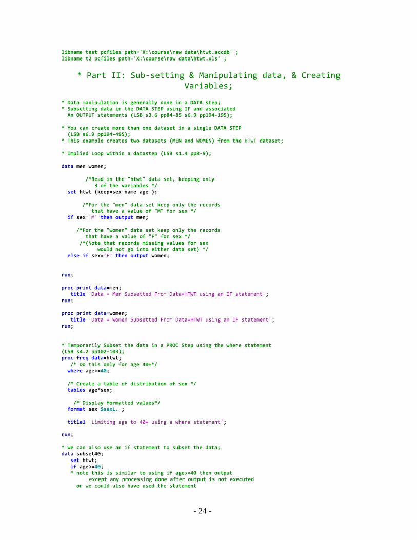
libname test pcfiles path='X:\course\raw data\htwt.accdb' ; libname t2 pcfiles path='X:\course\raw data\htwt.xls' ;

* Part II: Sub-setting & Manipulating data, & Creating Variables;

* Data manipulation is generally done in a DATA step; * Subsetting data in the DATA STEP using IF and associated An OUTPUT statements (LSB s3.6 pp84-85 s6.9 pp194-195); * You can create more than one dataset in a single DATA STEP (LSB s6.9 pp194-495); * This example creates two datasets (MEN and WOMEN) from the HTWT dataset; * Implied Loop within a datastep (LSB s1.4 pp8-9); data men women; /*Read in the "htwt" data set, keeping only 3 of the variables */ set htwt (keep=sex name age ); /*For the "men" data set keep only the records that have a value of "M" for sex */ if sex='M' then output men; /*For the "women" data set keep only the records that have a value of "F" for sex */ /*(Note that records missing values for sex would not go into either data set) */ else if sex='F' then output women; run; proc print data=men; title 'Data = Men Subsetted From Data=HTWT using an IF statement'; run; proc print data=women; title 'Data = Women Subsetted From Data=HTWT using an IF statement'; run; * Temporarily Subset the data in a PROC Step using the where statement (LSB s4.2 pp102-103); proc freq data=htwt; /* Do this only for age 40+*/ where age>=40; /* Create a table of distribution of sex */ tables age*sex; /* Display formatted values*/ format sex $sexL. ; title1 'Limiting age to 40+ using a where statement'; run; * We can also use an if statement to subset the data; data subset40; set htwt; if age>=40; * note this is similar to using if age>=40 then output except any processing done after output is not executed or we could also have used the statement

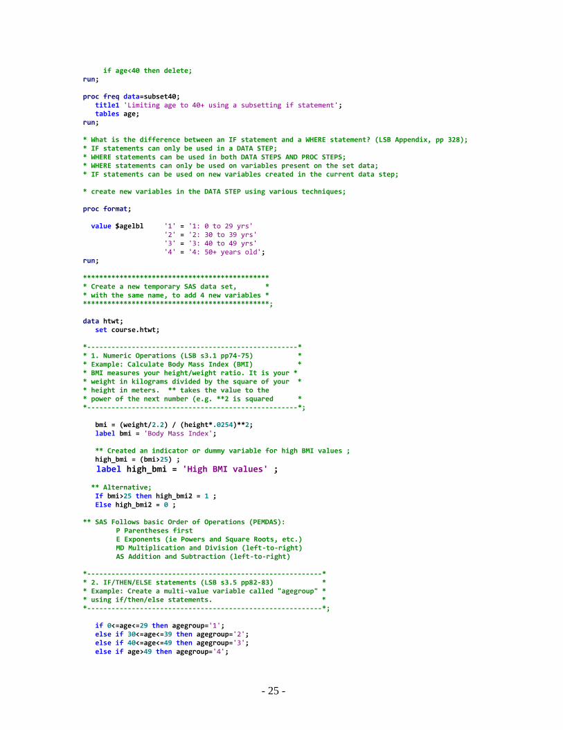
- 25 -

if age<40 then delete; run; proc freq data=subset40; title1 'Limiting age to 40+ using a subsetting if statement'; tables age; run; * What is the difference between an IF statement and a WHERE statement? (LSB Appendix, pp 328); * IF statements can only be used in a DATA STEP; * WHERE statements can be used in both DATA STEPS AND PROC STEPS; * WHERE statements can only be used on variables present on the set data; * IF statements can be used on new variables created in the current data step; * create new variables in the DATA STEP using various techniques; proc format; value $agelbl '1' = '1: 0 to 29 yrs' '2' = '2: 30 to 39 yrs' '3' = '3: 40 to 49 yrs' '4' = '4: 50+ years old'; run; ********************************************** * Create a new temporary SAS data set, * * with the same name, to add 4 new variables * **********************************************; data htwt; set course.htwt; *----------------------------------------------------* * 1. Numeric Operations (LSB s3.1 pp74-75) * * Example: Calculate Body Mass Index (BMI) * * BMI measures your height/weight ratio. It is your * * weight in kilograms divided by the square of your * * height in meters. ** takes the value to the * power of the next number (e.g. **2 is squared * *----------------------------------------------------*; bmi = (weight/2.2) / (height*.0254)**2; label bmi = 'Body Mass Index'; ** Created an indicator or dummy variable for high BMI values ; high_bmi = (bmi>25) ;

label high_bmi = 'High BMI values' ; ** Alternative; If bmi>25 then high_bmi2 = 1 ; Else high_bmi2 = 0 ; ** SAS Follows basic Order of Operations (PEMDAS):

P Parentheses first E Exponents (ie Powers and Square Roots, etc.) MD Multiplication and Division (left-to-right) AS Addition and Subtraction (left-to-right)

*----------------------------------------------------------* * 2. IF/THEN/ELSE statements (LSB s3.5 pp82-83) * * Example: Create a multi-value variable called "agegroup" * * using if/then/else statements. * *----------------------------------------------------------*; if 0<=age<=29 then agegroup='1'; else if 30<=age<=39 then agegroup='2'; else if 40<=age<=49 then agegroup='3'; else if age>49 then agegroup='4';

- 26 -

/* label one of the new variables */ label agegroup = 'Age grouped into 4 categories'; *------------------------------------------------------------* * 3. Functions (LSB s3.2-s3.4 pp76-81) * * SAS provides a large number of built-in functions to help * * you create new variables from old variables. * * Use the SAS help to find a list of SAS function categories.* * * * Numeric Function Examples: * LOG function takes the log to the base e * * ROUND returns a rounded value of a provided variable * * EXP Returns the value of the exponential function. * ABS Returns the absolute value * MOD Returns the remainder from the division of the first argument by the second argument, fuzzed to avoid most unexpected floating-point results. * SQRT Returns the square root * RANUNI, RANNOR, RANPOI,,, all return random values * * Numeric functions typically ignore missing values unlike * normal mathematical expressions *------------------------------------------------------------*; log_weight=log(weight); rounded_log = round(log_weight,.01) ; *---------------------------------------------------------------* * String Function Example: * SUBSTR extract a portion of variable. * * UPCASE returns an uppercase string * * COMPRESS Compresses characters or spaces out of a string * CAT, CATS, CATX Concatenate two or more variables * TRIM Removes trailing values, LEFT/RIGHT justify a string * LENGTH returns the length of a variable * SCAN scans a string variable for ‘words’ *---------------------------------------------------------------*; name3=substr(name,1,3); up_name = upcase(name) ; run; proc freq data=htwt; tables age * agegroup /list missing; format agegroup $agelbl.; /* add labels to the values of the new variables */ title1 'The height/weight data set'; title2 'Check new age group variable against original age variable'; run; **** NOTE: PROC MEANS excludes the observations with a missing class variable value from the analysis unless the / missing class statement option is used. ; proc means data=htwt n nmiss mean; title2 'Mean Value of BMI Classified by Age Group'; class agegroup; var bmi high_bmi; format agegroup $agelbl.; run; proc contents data=htwt; title2; /* remove 2nd title for remaining procs */ run; proc print data=htwt (obs=10); run;

- 27 -

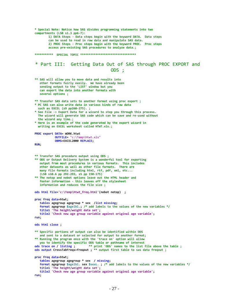
* Special Note: Notice how SAS divides programming statements into two compartments (LSB s1.3 pp6-7): 1) DATA Steps - Data steps begin with the keyword DATA. Data steps can be used to read in raw data and manipulate SAS data. 2) PROC Steps - Proc steps begin with the keyword PROC. Proc steps access pre-existing SAS procedures to analyze data.; *********** SPECIAL TOPIC *********************************

* Part III: Getting Data Out of SAS through PROC EXPORT and ODS ;

** SAS will allow you to move data and results into other formats fairly easily. We have already been sending output to the 'LIST' window but you can export the data into another formats with several options ; ** Transfer SAS data sets to another format using proc export ; * PC SAS can also write data in various kinds of raw data such as EXCEL (s9 pp260-275). ; * See File -> Export Data for a wizard to step you through this process. The wizard will generate SAS code which can be save and re-used without the wizard any time.; * Here is an example of the code generated by the export wizard in writing an EXCEL worksheet called HTWT.xls.; PROC export DATA= WORK.htwt OUTFILE= "c:\Temp\htwt.xls" DBMS=EXCEL2000 REPLACE; RUN;

** Transfer SAS procedure output using ODS ; ** ODS or Output Delivery System is a wonderful tool for exporting output from most procedures in various formats. This includes other datasets as well as other file formats. There are many file formats including html, rtf, pdf, xml, etc... (LSB s10.6 pp 292-293, s5 pp 150-175) ** The notop and nobot options leave out the HTML header and footer information - this leaves off the stylesheet information and reduces the file size ; ods html file='c:\Temp\htwt_freq.html'(nobot notop) ; proc freq data=htwt; tables agegroup agegroup * sex /list missing; format agegroup $agelbl.; /* add labels to the values of the new variables */ title1 'The height/weight data set'; title2 'Check new age group variable against original age variable'; run; ods html close ; ** Specific portions of output can also be identified within ODS and sent to a dataset or selected for output to another format; ** Running the program once with the 'trace on' option will allow you to identify the specific ODS table or pathname of interest ods trace on / listing ; ** print 'ODS' names to the list file above the table ; ods output CrossTabFreqs=freqout ; ** output first table to sas data freqout ; proc freq data=htwt; tables agegroup agegroup * sex / missing; format agegroup $agelbl. sex $sexL. ; /* add labels to the values of the new variables */ title1 'The height/weight data set'; title2 'Check new age group variable against original age variable'; run;

- 28 -

ods output close ; *** Turn everything back to the way it was ; ods trace off ; title1 'Frequency Cross Tables from HTWT' ; title2 'ODS Frequency Output Dataset' ; proc print data=freqout ; run; title ; *** Run a regression model and ouptut the parameters, estimates, and R-sq values to a single data file ; title1 'Regression with the Height/Weight datset' ; title2 'Does weight depend on age and height' ; *** Run once with 'Trace on' to get the ODS objects to place into SAS datasets ; ods trace on /listing ; *** Using the ODS names output the statistics and estimates into a data files ; ods output fitstatistics=fitstat parameterEstimates=paramest ; *** Run the regresion requesting the basic parameters in an output data file. Probabilities and Rsq values need to be pulled using ODS ; proc reg data=htwt outest=param_out ; model weight=age height ; quit; *** quit is used here since proc reg can be run interactively running each statement immediately *** Turn off ODS trace and ODS output ; ods output off ; ods trace off ; *** Parameter estimates from the regression ; proc print data=param_out ; title2 'Parameter Estimates from regression' ; run ; *** build a data file from ODS ouput for R square values ; data rsquare(keep=rsqr adj_rsq) ; set fitstat(where=(label2='R-Square') rename=(nValue2=rsqr)); set fitstat(where=(label2='Adj R-Sq') rename=(nValue2=adj_rsq)) ; proc print data=rsquare ; title2 'R-Square Values from regression' ; run; *** Build a data file that contains probabilities from ODS output ; data prob(keep=intercept_p age_p height_p) ; set paramest(where=(Variable='Intercept') rename=(probt=intercept_p)) ; set paramest(where=(Variable='age') rename=(probt=age_p)) ; set paramest(where=(Variable='height') rename=(probt=height_p)) ; run; proc print data=prob ; title2 'Probabilities from regression' ; run; *** Combine all of the data files together into a single file. Since they are all one record a merge is fine to do in this case also consider using if _n_=1 or multiple set statements ; data param ; merge param_out rsquare prob ; run; proc print data=param ; title2 'Combined Estimates, Probabilities and R-Square Values from regression' ; run;

- 29 -

Example 3 * f=htwt_example3.sas * * Part I. SAS Options (Printing) * * Part II. Sorting Data with PROC SORT * * Part III. Using SET to concatenate multiple SAS data sets * * Part IV. Using MERGE to add variables to a SAS data set * * Part V. Using PROC FORMAT and the PUT function to create new variables * * Part VI. Type conversions with put/input * *********************************************************************;

* Part I: SAS Options (printing); ** The SAS options statement can be used to change the way SAS works (LSB s1.13 pp26-27) ; options pageno=1; ** Printing - linesize/page size options. 1. Set the Page Setup (landscape/portrait and margins) 2. Set the Print Setup (including the font) Check the linesize/pageszie in the print setup. 3. Set the line and page size options to match print setup.; options ps=50 ls=130 ; /** Common SAS Options Dataset Options System Options Used in parentheses after DS Name Used with options statement e.g. Course.htwt(obs=5) ; e.g. options obs=100 ; drop= obs= keep= ps= obs= ls= in= fmterror/nofmterr where= mergnoby= compress= source/nosource **/

* Part II: Sorting Data with Proc Sort; * PROC SORT is used to sort a data set on specified variables (LSB s4.3 pp104-105).; ******************************************************* * This program sorts the data by name and creates a * * listing of the values of 3 variables (name being * * placed in the first column) for the first 10 records.* * The resulting output is displayed in alphabetical * * order by name. * *******************************************************; libname course 'X:\course\data'; data htwt; set course.htwt; run; proc sort data=htwt; by name ; run; *** Use ID statement to label printed observations in place of the observation number; proc print data=htwt (obs=10); id name; var sex age; title1 'PROC PRINT: Example 3'; title2 'Where the data set is sorted by name'; run;

- 30 -

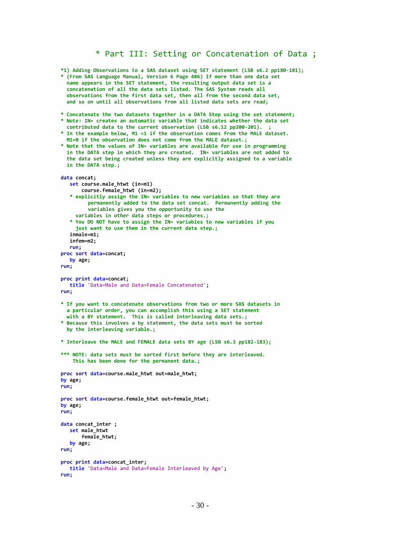
* Part III: Setting or Concatenation of Data ; *1) Adding Observations to a SAS dataset using SET statement (LSB s6.2 pp180-181); * (From SAS Language Manual, Version 6 Page 486) If more than one data set name appears in the SET statement, the resulting output data set is a concatenation of all the data sets listed. The SAS System reads all observations from the first data set, then all from the second data set, and so on until all observations from all listed data sets are read; * Concatenate the two datasets together in a DATA Step using the set statement; * Note: IN= creates an automatic variable that indicates whether the data set contributed data to the current observation (LSB s6.12 pp200-201). ; * In the example below, M1 =1 if the observation comes from the MALE dataset. M1=0 if the observation does not come from the MALE dataset.; * Note that the values of IN= variables are available for use in programming in the DATA step in which they are created. IN= variables are not added to the data set being created unless they are explicitly assigned to a variable in the DATA step.; data concat; set course.male_htwt (in=m1) course.female_htwt (in=m2); * explicitly assign the IN= variables to new variables so that they are permanently added to the data set concat. Permanently adding the variables gives you the opportunity to use the variables in other data steps or procedures.; * You DO NOT have to assign the IN= variables to new variables if you just want to use them in the current data step.; inmale=m1; infem=m2; run; proc sort data=concat; by age; run; proc print data=concat; title 'Data=Male and Data=Female Concatenated'; run; * If you want to concatenate observations from two or more SAS datasets in a particular order, you can accomplish this using a SET statement with a BY statement. This is called interleaving data sets.; * Because this involves a by statement, the data sets must be sorted by the interleaving variable.; * Interleave the MALE and FEMALE data sets BY age (LSB s6.3 pp182-183); *** NOTE: data sets must be sorted first before they are interleaved. This has been done for the permanent data.; proc sort data=course.male_htwt out=male_htwt; by age; run; proc sort data=course.female_htwt out=female_htwt; by age; run; data concat_inter ; set male_htwt female_htwt; by age; run; proc print data=concat_inter; title 'Data=Male and Data=Female Interleaved by Age'; run;

- 31 -

*** NOTE: If Tables only need to be concatenated without processing then proc append may be a more appropriate way to combine data.

* Part IV. Merging or adding variables; *2) Adding VARIABLES to a SAS dataset using MERGE - two datasets with a common merge key and different variables (LSB s6.4-6.5 pp184-187) Data sets are generally (though not necessarily) merged together using a merge key. A merge key is a variable that is common to both data sets - i.e. the merge key must have the same name and length on both data sets; * Both data sets must be sorted by the merge key; * A one-to-one merge describes the case where both data sets have one observation for every value of the merge key; * A common error is forgetting to use a BY statement in the merge. SAS by default does not report an error in this case. Adding the MERGENOBY option will either provide a warning or an error.; options mergenoby=warn ; * Add the variable REGION to the HTWT data set; data htwt; set course.htwt; run; data htwt_reg; set course.htwt_reg; run; proc sort data=htwt; by name; run; proc print data=htwt; title 'Merge Data Set #1: Data=HTWT'; run; proc sort data=htwt_reg; by firstname; run; proc print data=htwt_reg; title 'Merge Data Set #2: Data=HTWT_REG'; run; * In a merge, both data sets can contribute variables to the same observation; * The IN= variables (m1 and m2) will indicate which data sets contributed to each observation. The variable FIRSTNAME must be renamed to NAME so that the two data sets have a common merge key; data mer; merge htwt (in=m1) htwt_reg (in=m2 rename=(firstname=name)); by name; *** explicitly assign in= variables to the variables in_one and in_two so they are available in data set mer even after the data step is complete; in_one=m1; in_two=m2; run; proc print data=mer; title 'Merged Data Set: data=MER'; run; *3) Match merging - two datasets with a common merge key and different variables and different number of observations. In the end we will see those individuals that are over 30 years old and live in Winnipeg.;

- 32 -

*** Subset the HTWT dataset using a WHERE statement ; data htwt_ov30; set course.htwt; where age>30 ; run; ** Subset the HTWT_REG dataset selecting only those who are from Winnipeg; data htwt_wpg; set course.htwt_reg ; where region='Winnipeg' ; run; proc sort data=htwt_ov30; by name; run; proc print data=htwt_ov30; title 'Merge Data Set #1: Data=HTWT Where age>30'; run; proc sort data=htwt_wpg; by firstname; run; proc print data=htwt_wpg; title 'Merge Data Set #2: Data=HTWT_REG Where Region=Winnipeg'; title2 'Note Number of Observations'; run; data mer; merge htwt_ov30 (in=m1) htwt_wpg (in=m2 rename=(firstname=name)); by name; in_one=m1; in_two=m2; run; proc print data=mer; title 'Merged Data Set: data=MER All Observations'; run; ** Limit data to just those over 30 and living in Winnipeg ; data mer; merge htwt_ov30 (in=m1) htwt_wpg (in=m2 rename=(firstname=name)); by name; if m1=1 & m2=1 ; ** Subsetting if requires contribution from both data sets ; run; proc print data=mer; title 'Merged Data Set: data=MER Selecting Only Observation Present on Both Merged Datasets'; run; *4) One-to-many match merging (LSB s6.5 pp186-187, s6.6-6.7 pp188-191) ; * One-to-many merging refers to the case where one data set has one observation for each value of the merge key and the other data set has more than one observation for each value of the merge key.; * Create a dataset with one observation per value of sex using Proc Means; * Note: noprint option suppresses the printed output from Proc MEANS nway option limits the output to the highest level of interaction among CLASS variables; proc means data=course.htwt noprint nway; class sex; var age; output out=mage mean=mean_age; ** / autoname was not used in this example ; run;

- 33 -

proc print data=mage; title 'Mean age by sex Produced by Proc Means'; run; *** Note that the original data file is not sorted; **** use out= option to name the sorted data set and not overwrite the original; proc sort data=course.htwt out=htwt ; by sex; run; proc sort data=mage; by sex; run; data mer; merge htwt (in=m1) mage (in=m2 keep=sex mean_age); by sex; * create a variable that is equal to 1 if age is greater than the mean value of age (for each sex) and 0 otherwise. This is often called an indicator variable.; if age > mean_age then hi_age=1; else if 0 < age <= mean_age then hi_age=0 ; else hi_age=.; label hi_age='Age Greater than Mean Value of Age for Each Sex'; run; proc print data = mer; title 'Data = Mer - Adding Mean age by Sex'; run; proc means data=mer n sum mean; title 'Proportion of Observations with Age Greater than Mean Age Value'; class sex; var hi_age; run; /* Set and Merge - to the tune of Deep and Wide. Set and Merge Set and Merge There's a Data Step for Set and Merge <repeat> */

* Part V: Use of Put() with formats for creating variables; * Creating a variable using a format statement; * Previously we learned that formats can be used to label values of variables and to aggregate values of variables into groups. The example from last class used IF/THEN/ELSE statements to group age into 4 groups.; * Though it is perfectly acceptable to use IF/THEN/ELSE, now we are going to show you how to use a fairly advanced technique to do the same thing. ; * This advanced technique uses formats along with the PUT Function to create a new grouping variable. This is mainly useful when you wish to group a large number of levels into a relatively small number of groups. A good example would be grouping the 18,000+ Winnipeg postal codes into the 12 Winnipeg areas. ;

- 34 -

* PUT and INPUT functions are discussed in general in the LSB, s11.8 (pp310-311). The use of these functions with user-defined formats is not discussed ; * Example: Creating an Age Group Variable using a format and the PUT function; * Recall that whenever we want to use a format, we must first create the format using PROC FORMAT; proc format; * This format groups age into 4 groups; value agegrpf 00-29 = '1' 30-39 = '2' 40-49 = '3' 50-high = '4'; * This format labels the age group variable; value $agegrpl '1' = '1: 0-29 years' '2' = '2: 30-39 years' '3' = '3: 40-49 years' '4' = '4: 50+ years'; run; data htwt; set course.htwt; * You can create a grouping variable with a format by using the PUT function.; * The result of the PUT function is always a character variable.; * The put function puts the formatted value of Age into the new variable AGEGRP. The new variable AGEGRP takes on the values '1','2','3','4'; agegrp = put (age,agegrpf.); label agegrp = 'Age Group'; *** You can do this using if/then/else statements as well (see last class); if 0<=age<=29 then agegroup='1'; else if 30<=age<=39 then agegroup='2'; else if 40<=age<=49 then agegroup='3'; else if age>49 then agegroup='4'; run; proc freq data=htwt; title 'Using the PUT function and a FORMAT to create a new Variable (AGEGRP)'; title2 'NOTE that AGEGRP has had the Labelling Format $AGEGRPL applied to it'; tables agegrp*age/list ; * note that by applying the labeling format $AGEGRPL to the new variable AGEGRP we see the formatted values of AGEGRP instead of the underlying values of '1','2','3','4'; format agegrp $agegrpl.; run; ** Formatted values and class statements with output data (may be skipped). * You may well ask why not just apply the grouping format AGEGRPF directly to AGE when analyzing it? Or, what is the advantage of using a grouping variable when a grouping format will do the same thing? The answer is somewhat complex. When the object is just to create a report, a grouping format applied directly to the variable for analysis will be adequate. When the object of the analysis is to produce an output SAS dataset by the grouped variable, you need to be concerned about the underlying value of the grouped variable when a grouping format is applied at the time of analysis.; * Here is an example of applying the grouping format AGEGRPF directly to age for reporting and for creating a SAS output dataset; title 'Applying the Grouping Format AGEGRPF Directly to AGE at Analysis Time'; title2 'NOTE That the Values 1-4 appear as the Formatted Values of Age';

- 35 -

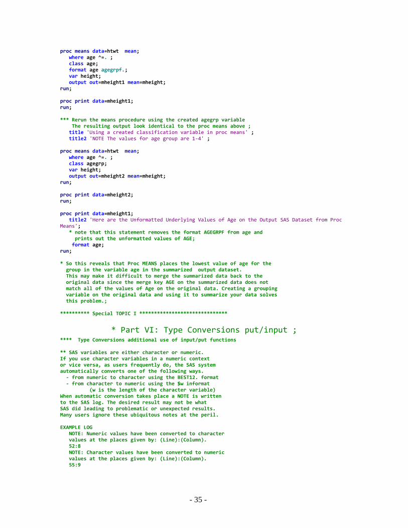
proc means data=htwt mean; where age ^=. ; class age; format age agegrpf.; var height; output out=mheight1 mean=mheight; run; proc print data=mheight1; run; *** Rerun the means procedure using the created agegrp variable The resulting output look identical to the proc means above ; title 'Using a created classification variable in proc means' ; title2 'NOTE The values for age group are 1-4' ; proc means data=htwt mean; where age ^=. ; class agegrp; var height; output out=mheight2 mean=mheight; run; proc print data=mheight2; run; proc print data=mheight1; title2 'Here are the Unformatted Underlying Values of Age on the Output SAS Dataset from Proc Means'; * note that this statement removes the format AGEGRPF from age and prints out the unformatted values of AGE; format age; run; * So this reveals that Proc MEANS places the lowest value of age for the group in the variable age in the summarized output dataset. This may make it difficult to merge the summarized data back to the original data since the merge key AGE on the summarized data does not match all of the values of Age on the original data. Creating a grouping variable on the original data and using it to summarize your data solves this problem.; ********** Special TOPIC I ******************************

* Part VI: Type Conversions put/input ; **** Type Conversions additional use of input/put functions ** SAS variables are either character or numeric. If you use character variables in a numeric context or vice versa, as users frequently do, the SAS system automatically converts one of the following ways. - from numeric to character using the BEST12. format - from character to numeric using the $w informat (w is the length of the character variable) When automatic conversion takes place a NOTE is written to the SAS log. The desired result may not be what SAS did leading to problematic or unexpected results. Many users ignore these ubiquitous notes at the peril. EXAMPLE LOG NOTE: Numeric values have been converted to character values at the places given by: (Line):(Column). 52:8 NOTE: Character values have been converted to numeric values at the places given by: (Line):(Column). 55:9

- 36 -

Implicit conversions are very slow. To ensure appropriate results when converting between character and numeric data, use the PUT or INPUT function to control type conversion. Often to save disk space indicator variables have been coded as character 0/1. To use these variables in analysis such as a logistic regression they will need to be converted. INPUT: Letters or strings that contain letters are set to missing and and an 'Invalid argument' note is written to the log. PUT Missing numerics are written as a period '.' ; ; *** Setup some data so we can see what the conversions look like. data riw_test ; input @1 flag $1. @3 code 4. @8 riw $5. ; label riw='Resource Intensity' code='Coded Diagnostic Group' flag='Binary flag' ; datalines ; 1 0010 2.474 0 100 0.924 1 006 4.289 0 060 4.289 1 600 1.029 0 113 0.467 l 317 0613 ; run; *** Codes in the above code 006 (Amebiasis), 060 (yellow fever), 600 (Hyperplasia of prostate) data calc ; set riw_test ; *** Calculations on a character string returns a numeric but SAS does the conversion. In the above data the last record was accidentally missing the period.; cost = riw * 2234.00 ; *** Character operations (concatination) returns a character string but not what is expected. The input above caused problems as well. ; CDG = "CDG " || code ; run; proc print data=test ; run; *** Running a proc means to get the proportion of the records with a true response does not work since the variable is character ; proc means data=test ; var flag ; run; *** Re do the conversions above using input/put functions; data calc ; set riw_test ;

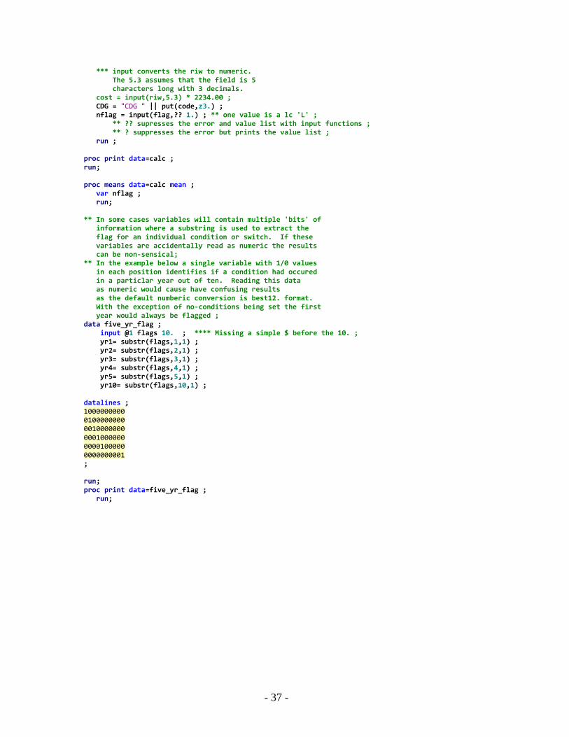
- 37 -

*** input converts the riw to numeric. The 5.3 assumes that the field is 5 characters long with 3 decimals. cost = input(riw,5.3) * 2234.00 ; CDG = "CDG " || put(code,z3.) ; nflag = input(flag,?? 1.) ; ** one value is a lc 'L' ; ** ?? supresses the error and value list with input functions ; ** ? suppresses the error but prints the value list ; run ; proc print data=calc ; run; proc means data=calc mean ; var nflag ; run; ** In some cases variables will contain multiple 'bits' of information where a substring is used to extract the flag for an individual condition or switch. If these variables are accidentally read as numeric the results can be non-sensical; ** In the example below a single variable with 1/0 values in each position identifies if a condition had occured in a particlar year out of ten. Reading this data as numeric would cause have confusing results as the default numberic conversion is best12. format. With the exception of no-conditions being set the first year would always be flagged ; data five_yr_flag ; input @1 flags 10. ; **** Missing a simple $ before the 10. ; yr1= substr(flags,1,1) ; yr2= substr(flags,2,1) ; yr3= substr(flags,3,1) ; yr4= substr(flags,4,1) ; yr5= substr(flags,5,1) ; yr10= substr(flags,10,1) ; datalines ; 1000000000 0100000000 0010000000 0001000000 0000100000 0000000001 ; run; proc print data=five_yr_flag ; run;

- 38 -

Example 4 * f=htwt_example4.sas * * * Session 4 * * Part I. By Group Processing (First, Last, retain) * * Part II. Groups of Variables & Array processing * * Session 5 * * Part I. Date Time Processing * * Part II. SQL * ************************************; ** reset page number. Set page size and line size for landscape printing ; options pageno=1 ps=41 ls=127; libname course 'X:\course\data'; %include 'X:\course\Formats\newfmts.sas' ;

* Part I: By group processing for Longitudinal Data ; * By-Group Processing in a DATA step (LSB s6.15 pp206-207) ------------------------------------ ; * A BY-group is a group of one or more observations with the same value of the BY variable(s). For example, if you sort a data set by Name, then a BY-group is all of the observations with NAME='Deborah'.; * A BY-group may also be designated by more than one BY variable. For example, if you sort a data set by NAME and AGEGRP, one of the BY-groups could be NAME='Deborah' and AGEGRP=00-19.; * To process a data set using a BY-group, you must use a BY statement in a DATA step. SAS will expect the observations to be in order by the value of the variables specified in the BY statement.; * When processing a data set using a BY-group, SAS generates two automatic temporary variables for each variable specified in the BY statement: FIRST.variable and LAST.variable.; * These variables are available for programming in the DATA step, but are not permanently added to the data set unless they are explicitly assigned to a variable in the data step.; * FIRST.variable =1 for the first observation in a BY-group and 0 otherwise; * LAST.variable =1 for the last observation in a BY-group and 0 otherwise; * If an observation is the first and last observation in a By-group (ie the By-group has only one observation in it) then FIRST.variable=1 and LAST.variable=1; *** Create a new data set for height and weight over time (age) for two individuals ; *** In this example we are using comma delimited data ; data htwt_long ; infile datalines dlm=',' dsd ; ** The infile statement tells SAS where the raw data records are found. This can be a separate file or inline using cards or datalines (LSB s2.4 pp36-37). In this case an infile is required because the data is in a delimited format. dlm - identifies the delimeter, dsd - tells SAS how to deal with multiple delimiters (LSB s2.15 pp58-59) ; informat name $10. ; *** Informats define how the variable should be read. This statement is generally used when the length of individual variables may not be constant over the whole file. If the length is known the informat can put on the input statement after the variable name (LSB s2.7-2.8 pp42-45, s2.21 pp70-71).; input name age height weight ; datalines ; Deborah,35,66,125

- 39 -

Deborah,34,66,133 Deborah,33,66,131 Deborah,30,66,130 Deborah,31,66,129 Deborah,32,66,128 Carl,35,70,140 Carl,32,70,155 Carl,36,70,155 Carl,34,70,157 Carl,33,70,160 Carl,37,70,160 ; run; * In order to process a data set BY NAME, it must first be sorted by NAME; * Usually another variable will need to be included to ensure that the order within each by group makes sense (e.g. date order) ; proc sort data=htwt_long; by name age; run; proc print data=htwt_long ; run; * SAS creates the temporary FIRST. and LAST. variables available to the DATA STEP when you indicate you want to process a dataset "by" some variable; data htwt_long; set htwt_long; * BY statement indicates the BY-group; by name; * FIRST. and LAST. variables are NOT permanently added to the dataset, unless they are explicitly assigned to a variable in the data set.; first_name=first.name; last_name=last.name; run; proc print data=htwt_long; title 'Processing HTWT data by Name'; var name first_name last_name age height weight; run; * SAS has two functions that allow for some basic longitudinal processing. LAG() function will return the value for a variable from the last record allowing comparisons with earlier records. The DIF() function is closely related that it will return the difference in a value between the current and a prior record. Both of these functions can identify more than just the prior record by using a number suffix (e.g. lag5() returns the value from the fifth prior record.; data lag ; set htwt_long ; by name ; lag_weight = lag(weight) ; weight_change = dif(weight) ; run; Proc print data=lag ; var name age height weight lag_weight weight_change ; run; * When using LAG() and DIF() functions it is important that the first value in each by group be re-set since it reflects the last value of the prior individual in the group. NOTE: The LAG() and DIF() functions should not usually be defined within an an if/then block ; data lag ; set htwt_long ; by name ; lag_weight = lag(weight) ; weight_change = dif(weight) ; *** reset first values in each by group. ; if first.name then do ; lag_weight = . ; weight_change = . ;

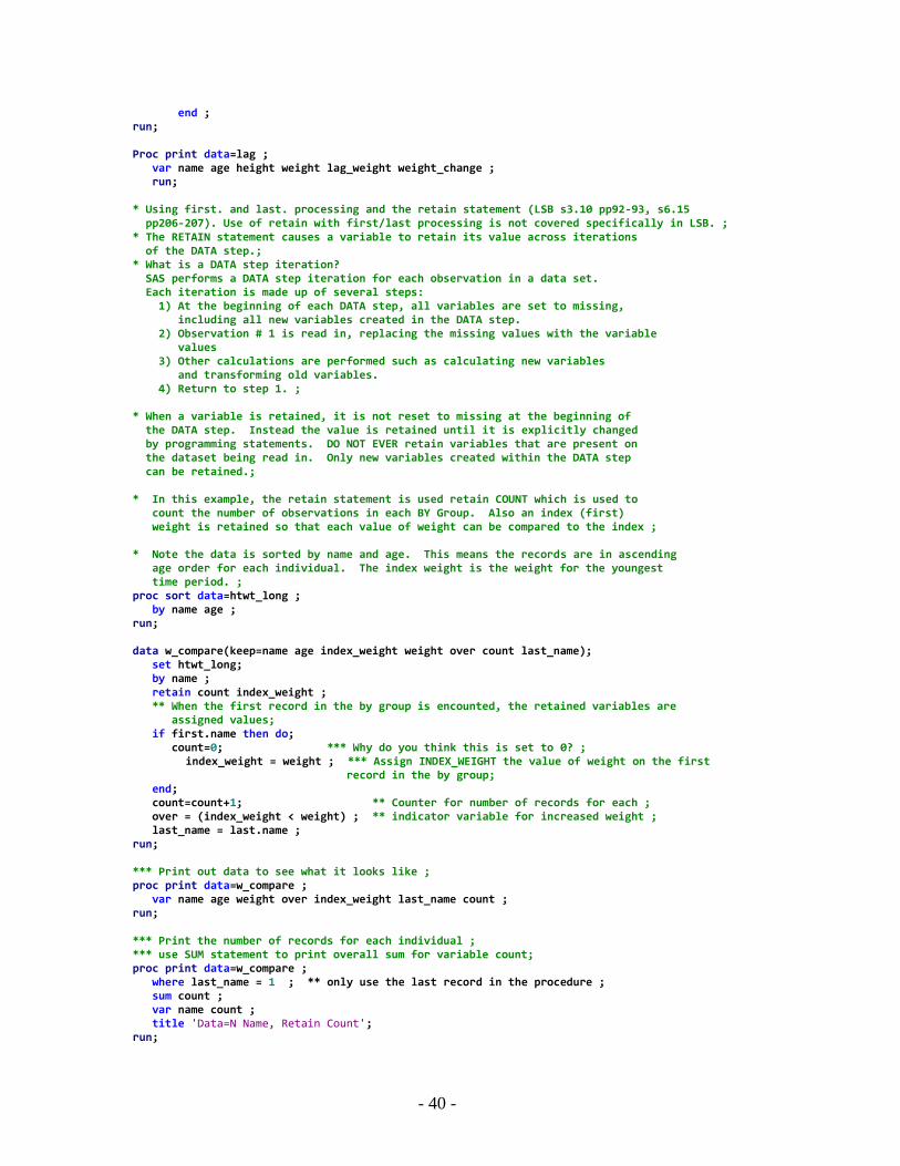
- 40 -

end ; run; Proc print data=lag ; var name age height weight lag_weight weight_change ; run; * Using first. and last. processing and the retain statement (LSB s3.10 pp92-93, s6.15 pp206-207). Use of retain with first/last processing is not covered specifically in LSB. ; * The RETAIN statement causes a variable to retain its value across iterations of the DATA step.; * What is a DATA step iteration? SAS performs a DATA step iteration for each observation in a data set. Each iteration is made up of several steps: 1) At the beginning of each DATA step, all variables are set to missing, including all new variables created in the DATA step. 2) Observation # 1 is read in, replacing the missing values with the variable values 3) Other calculations are performed such as calculating new variables and transforming old variables. 4) Return to step 1. ; * When a variable is retained, it is not reset to missing at the beginning of the DATA step. Instead the value is retained until it is explicitly changed by programming statements. DO NOT EVER retain variables that are present on the dataset being read in. Only new variables created within the DATA step can be retained.; * In this example, the retain statement is used retain COUNT which is used to count the number of observations in each BY Group. Also an index (first) weight is retained so that each value of weight can be compared to the index ; * Note the data is sorted by name and age. This means the records are in ascending age order for each individual. The index weight is the weight for the youngest time period. ; proc sort data=htwt_long ; by name age ; run; data w_compare(keep=name age index_weight weight over count last_name); set htwt_long; by name ; retain count index_weight ; ** When the first record in the by group is encounted, the retained variables are assigned values; if first.name then do; count=0; *** Why do you think this is set to 0? ; index_weight = weight ; *** Assign INDEX_WEIGHT the value of weight on the first record in the by group; end; count=count+1; ** Counter for number of records for each ; over = (index_weight < weight) ; ** indicator variable for increased weight ; last_name = last.name ; run; *** Print out data to see what it looks like ; proc print data=w_compare ; var name age weight over index_weight last_name count ; run; *** Print the number of records for each individual ; *** use SUM statement to print overall sum for variable count; proc print data=w_compare ; where last_name = 1 ; ** only use the last record in the procedure ; sum count ; var name count ; title 'Data=N Name, Retain Count'; run;

- 41 -

*** Calculate the proportion of measurements that the weight of the individual was over their index weight ; proc means data=w_compare mean ; class name ; var over weight ; title 'Proportion of records where weight was over the index for each individual' ; run; ** Can you think of another way to get the total number of records for each individual in a data set? ; ** If there are other methods to get counts, why do you think we would use first/last processing.? ; ** Using a datastep count is faster when there are many levels of the class or by variable (e.g. 5000 levels) ; ** First/Last processing can also be used for cumulating other kinds of variables in information across by groups. In this example we will follow the same program as above but we can count the number of times each person is over their index weight ; data w_compare(keep=name index_weight count over_counter percent_over ); set htwt_long; by name ; retain count index_weight over_counter ; ** When the first record in the by group is encounted, the retained variables are assigned values; if first.name then do; count=0; *** Why do you think this is set to 0? ; index_weight = weight ; *** Assign INDEX_WEIGHT the value of weight on the first record in the by group; over_counter = 0 ; end; count=count+1; ** Counter for number of records for each ; over = (index_weight < weight) ; ** indicator variable for increased weight ; over_counter = over_counter + over ; if last.name then do ; percent_over = (over_counter/count) * 100 ; output ; end ; run; *** Print out data to see what it looks like ; proc print data=w_compare ; var name count over_counter percent_over index_weight ; run;

* Part II. Groups of Variables & Array processing; *** Groups of Variables ------------------------ *** Using Groups of Variables with functions and arrays ; proc contents data=course.htwt_wide; run; proc print data=course.htwt_wide ; run ; * Many SAS functions can be used with groups of variables to get summary statistics and information (LSB s3.2 & s3.3, pp76-79. MIN(arg,arg) or MIN(of X1-Xn)

- 42 -

MAX(arg,arg) or MAX(of X1-Xn) SUM(arg,arg) or SUM(of X1-Xn) MEAN(arg,arg) or MEAN(of X1-Xn) Unlike normal arathmetic opperations SAS funcitions do not return a missing value when calculations are attempted on a missing. Missing values are skipped. ; ** Example: returning summary statistics from groups of similar variables; data wide ; set course. htwt_wide ; *** Use various statistical functions for getting summary values of weight ; count = n(of age1-age6) ; sum_weight = sum(of weight1-weight6) ; mean_weight = mean(of weight1-weight6) ; min_weight = min(of weight1-weight6) ; max_weight = max(of weight1-weight6) ; run; proc print data=wide ; title 'Summary Statistics using multiple variables and functions' ; var name count sum_weight mean_weight min_weight max_weight ; run; ** Transposing data (a side note since many people ask);

** Although SAS provides statistical functions for doing analysis over multiple

related variables it is often easier in SAS to have a single variable and multiple

records this is how most procedures 'expect' data to be formated. ;

** If necessary PROC Transpose or a datastep can be used to switch variables 'wise' data

to column 'wise' ;

** Proc Transpose example - transpose is done twice since there are two sets of variables

that need to be transposed. Once there are large number of records or fields using

a datastep to transpose might be more efficient ;

proc transpose data=course.htwt_wide out=wt_long prefix=weight;

by name ;

var weight1-weight6 ;

run;

proc transpose data=course.htwt_wide out=ag_long prefix=age;

by name ;

var age1-age6 ;

run;

data htwt_long ;

merge wt_long

ag_long(drop=_name_) ;

by name ; *** SAS will write a note that MERGE has repeats of by values ;

time = substr(_name_,7,1) ; ** the _name_ variable contains the original

variable name - get suffix ;

drop _name_ ;

run;

** Data Step transpose - this uses a 'Do' loop with an output to create a new record for

each variable in a dataset ;

data htwt_long(keep=name time weight age);

set course.htwt_wide ;

** Define the groups of variables to transpose ;

array wt{6} weight1-weight6 ;

array ag{6} age1-age6 ;

** re-assign each variable to a new variable and output a new

record for each array variable. ;

do time = 1 to 6 ;

weight = wt{time} ;

age = ag{time} ;

output ;

end ;

run;

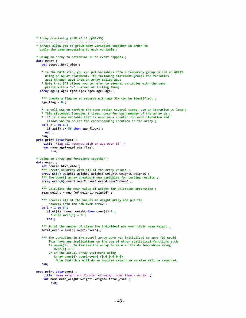
- 43 -

* Array processing (LSB s3.11 pp94-95) --------------------------------------- ; * Arrays allow you to group many variables together in order to apply the same processing to each variable.; * Using an array to determine if an event happens ; data event ; set course.htwt_wide ; * In the DATA step, you can put variables into a temporary group called an ARRAY using an ARRAY statement. The following statement groups the variables age1 through age6 into an array called ag.; * Note that SAS allows you to refer to several variables with the same prefix with a "-" instead of listing them; array ag{6} age1 age2 age3 age4 age5 age6 ; *** create a flag so so records with age 35+ can be identified. ; age_flag = 0 ; * To tell SAS to perform the same action several times, use an iterative DO loop.; * This statement iterates 6 times, once for each member of the array ag.; * 'i' is a new variable that is used as a counter for each iteration and allows SAS to select the corresponding location in the array ; do i = 1 to 6 ; if ag{i} >= 36 then age_flag=1 ; end ; run; proc print data=event ; title 'Flag all records with an age over 35' ; var name age1-age6 age_flag ; run; * Using an array and functions together ; data event ; set course.htwt_wide ; *** Create an array with all of the array values ; array wt{6} weight1 weight2 weight3 weight4 weight5 weight6 ; *** the over{} array creates 6 new variables for testing results ; array over{6} over1 over2 over3 over4 over5 over6 ; *** Calculate the mean value of weight for selection procession ; mean_weight = mean(of weight1-weight6) ; *** Process all of the values in weight array and put the results into the new over array ; do i = 1 to 6 ; if wt{i} > mean_weight then over{i}=1 ; * else over{i} = 0 ; end ; *** Total the number of times the individual was over their mean weight ; total_over = sum(of over1-over6) ; *** The variables in the over{} array were not initialized to zero (0) would This have any implications on the use of other statistical functions such As mean()?. Initialize the array to zero in the do loop above using Over{i} = 0 Or in the actual array statement using Array over{6} over1-over6 (0 0 0 0 0 0) Note that this will do an implied retain so an else will be required; run; proc print data=event ; title 'Mean weight and Counter of weight over time - Array' ; var name mean_weight weight1-weight6 total_over ; run;

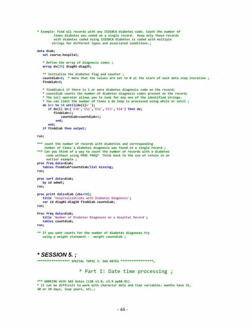
- 44 -

* Example: Find all records with any ICD10CA diabetes code. Count the number of times diabetes was coded on a single record. Keep only those records with diabetes coded Using ICD10CA Diabetes is coded with multiple strings for different types and associated conditions.; data diab; set course.hospital; * Define the array of diagnosis codes ; array dx(25) diag01-diag25; ** Initialize the diabetes flag and counter ; countdiab=0; * Note that the values are set to 0 at the start of each data step iteration ; finddiab=0; * finddiab=1 if there is 1 or more diabetes diagnosis code on the record; * countdiab counts the number of diabetes diagnosis codes present on the record; * The in() operator allows you to look for any one of the identified strings. * You can limit the number of times a do loop is processed using while or until ; do i=1 to 10 until(dx{i}=''); if dx(i) in:('E10','E11','E12','E13','E14') then do; finddiab=1; countdiab=countdiab+1; end; end; if finddiab then output; run; *** count the number of records with diabeties and corresponding number of times a diabetes diagnosis was found in a single record ; *** Can you think of a way to count the number of records with a diabetes code without using PROC FREQ? Think back to the use of retain in an earlier example ; proc freq data=diab; tables finddiab*countdiab/list missing; run; proc sort data=diab; by id admdt; run; proc print data=diab (obs=50); title 'Hospitalizations with Diabetes Diagnosis'; var id diag01-diag10 finddiab countdiab; run; Proc freq data=diab; title 'Number of Diabetes Diagnoses on a Hospital Record'; tables countdiab; run; ** If you want counts for the number of diabetes diagnoses try using a weight statement - weight countdiab ;

* SESSION 5. ; ****************** SPECIAL TOPIC I: SAS DATES ******************;

* Part I: Date time processing ; *** WORKING With SAS Dates (LSB s3.8, s3.9 pp88-91) * It can be difficult to work with character date and time variables: months have 31, 30 or 28 days, leap years, etc.;

- 45 -

* SAS has special numeric date variables called SAS Dates that allow you to add, subtract and do other calculations without worrying about the number of days in a month or year.; * SAS dates represent the number of days since (or before) January 1, 1960. Below are some examples of SAS dates: Date SAS Date January 1, 1960 0 January 1, 1961 366 January 1, 1959 -365 March 31, 2007 17256 March 31, 2008 17622 * The difference between March 31, 2007 and March 31, 2008 = 17622-17256 = 366; * SAS "knows" that 2008 is a leap year and includes that extra day in the calculation; * http://support.sas.com/techsup/technote/ts668.html ; A little side note: The earliest date that is valid in SAS software is January 1, 1582 -- SAS software uses the Gregorian calendar. That is the year that France, Italy, Luxembourg, Portugal, and Spain replaced the Julian calendar with the Gregorian. (The Gregorian calendar was first implemented so that the day after October 4, 1582 was October 15, 1582. Nevertheless, SAS software recognizes 31 days in the month of October, 1582.) While the rest of Roman Catholic Europe switched shortly after 1582, the United Kingdom and its colonies did not move to the Gregorian calendar until 1752. Many other countries switched even later, including the Soviet Union in 1918 and Greece in 1923. Some historic dates therefore might be handled in a misleading manner -- a problem which, it should be noted, is true of any use of SAS dates in such instances. data dates; infile 'X:\course\Raw Data\dates.txt' firstobs=2 ; input @1 ident $8. @11 sex $1. @13 sasdatedob yymmdd8. /*** read data directly into SAS Date format ***/ @23 admdate $8. @33 sepdate $8. ; *** create SAS date variables from character variables using INPUT functions (LSB s11.8 pp310-311) and SAS Date/Time INFORMATS (LSB s2.8 pp44-45).; *** INPUT functions are similar to PUT functions, except that INPUT returns a numeric value while PUT returns a character value. Date values are often provided as character strings and must be converted to SAS dates either with an input statement (see below) or when reading the data with an input statement.; sasdateadm = input(admdate,yymmdd8.); sasdatesep = input(sepdate,yymmdd8.); label sasdateadm = 'Date of Hospital Admission, SAS Date'; label sasdatesep = 'Date of Hospital Separation, SAS Date'; format sasdateadm date9. sasdatesep yymmdd10. ; *** obtain the month of admission from the SAS Date variable using the MONTH function; month_adm = month(sasdateadm); month_sep = month(sasdatesep); label month_adm = 'Month of Hospital Admission'; label month_sep = 'Month of Hospital Separation'; *** obtain the Day of the week for admission from SAS dates using weekday function The SAS week starts with Sunday being 1 ; weekday = weekday(sasdateadm) ; *** Simple difference between two date variables is the number of days ; los = sasdatesep - sasdateadm ; *** Intervals measurements are often useful for determining the passage of time e.g. the number of weeks (number of Sundays) or months (1 day of each month) between two dates. Intervals are determined using the INTCK() function. Number of week intervals between the dates determined by Monday. ; weeks_passed = intck('week.2', sasdateadm, sasdatesep) ; *** often you may want to calculate the number of days between an event and a constant index date, where the event date is a variable in the data, but the index date is a fixed day. You can enter in any fixed date as a SAS

- 46 -

date in the following using: 'DDmonYYYY'd The 'd' trailing the quoted string indicates that the string is a SAS date; datediff = '01mar2004'd - sasdateadm; label datediff = 'Number of Days between Date of Admission and March 1, 2004'; *** Calculation of actual age - this is often done by dividing by 365.25 ; *** Floor takes the integer value from the decimal value ; agesep = floor(yrdif(sasdatedob,sasdateadm,'AGE')) ; label agesep='Age at Separation' sasdatedob='Date of Birth, SAS Date' ; format sasdatedob yymmdd10. ; run; *** SAS dates can be displayed many different ways using SAS Date/Time formats (LSB s4.6 pp110-111); proc print data = dates (obs=20) label; var admdate sasdateadm sepdate sasdatesep datediff sasdatedob agesep weekday los weeks_passed; title 'Character Dates and SAS Dates'; *** comment the line below to see different SAS date formats; format sasdateadm sasdatesep ; run; proc contents data=dates ; run; proc univariate data = dates; var month_adm month_sep; histogram /normal midpoints = 1 to 12 by 1; title 'Distribution of Hospital Stays by Month'; run; ****************** SPECIAL TOPIC II SQL Processing**************;

* Part II: SQL Processing ; * An alternative to some procedures and data step programming would be to use Proc SQL. We will not be covering this procedure in depth during this workshop but those familiar with SQL should know that it is available. Merges and sets can also be done with joins in Proc SQL but it is often more efficient do use base SAS data step processing. (LSB Appendix pp325-330, s6.3 pp182-183, s6.4 pp184-185); * SQL stands for Structured Query Language and was originally developed by IBM for extracting information from databases. SQL works on processing columns (variables) rather than observations (in an implied loop). * Procedure SQL commands Base SAS equivalent ; /* Proc SQL ; create DATA as (Data statement) Select (Keep & proc print & proc means statistics options) From <left/right join> (Set/merge statement) Where (on) (Where statement & By statement in merge) Group by (class statement) Having (post processing datastep from proc means) Order by ; (proc sort) quit ; */ * Statements in SQL need to go in the above order – it might be helpful to think of the saying: Some French Waiters Grow Healthy Oranges. There are many more capabilities and SQL commands avialable e.g. Unions (compare to SET). * There is a nice online summery of generic SQL found online: https://www.w3schools.com/SQL/deFault.asp The examples provided here need to go between the Proc SQL and Quit statements.; * Common problems: 1. When listing multiple variables and datasets they must be separated by commas.

- 47 -

2. An SQL command is one single statement. 3. Use of an alias for a permanent SAS datasets can be confusing. Since SQL uses a period ('.') to identify a table.field there needs to be a way for a permanent datasets (library.table) to be identified. In SAS SQL use the notation 'as' to identify an alias or short name to represent the permanent dataset. * Top reasons for using SQ 1. 'Fuzzy' merge 2. Join tables (esp multiple database with different keys) 3. Add summary data to groups/overall 4. Save steps on basic processing 5. Easier for other DB programmers to understand

6. Selections (Where) can use wild characters. * Where selections can include the comparison clauses: LIKE with wild characters represented by: an underscore (_) to represent a single character. a percent sign (%) to represent a string of characters. CONTAINS to search for a string within a string. ; ** Basic printed output ; proc sql ; select name, sex, height from course.htwt ; quit ; ** Basic query to create a male only file ; proc sql ; create table males as select name, age, sex, height, weight from course.htwt where sex='M'; quit ; ** Adding overall mean to every record in a dataset (from above) doing a calculation with a newly created variable, An * is used to identify all of the existing fields in the table.; proc sql ; create table test as select *, mean(weight) as meanwt, weight-(calculated meanwt) as diff from course.htwt ; quit ; proc print data=test(obs=10) ; title 'Data table created with Average LOS on each record using SQL' ; var name sex weight meanwt diff ; run; ** Adding mean age for each sex to every record in a dataset (from example prog 3 ; proc sql ; create table mage as select *, mean(age) as mage, age>(calculated mage) as high_age label='Age Greater than Mean Value of Age for Each Sex' from course.htwt group by sex order by age ; quit ; proc print data=mage ; title 'Data table created with Average AGE by sex using SQL' ; run; ** Joining two datasets together by key variables (from example prog 3) and printing results. When using multiple from tables SQL needs a way to identify the table name and the corresponding fields. In SQL a period in the select command is used to identify the table followed by the specific variable. In SAS a period is used to distinguish a library (location) and then a table name. In the following example this problem is resolved by providing an

- 48 -

Alternative name (short cut) using ‘as’ in the from line. Course.htwt_reg.region <- this is invalid SQL as the field identifier has two periods. This is resolved by identifying (course.htwt) as htwt_reg SQL will only ‘see’ htwt_reg.region because the course. Is replaced with The short alternative name. In practice the use of an alternative (alias) is only required if there are fields with the same name making a selection ambiguous.; title 'Data table created with a join by name/firstname using SQL' ; proc sql ; create table merged as select ahtwt.*, areg.region from course.htwt as ahtwt, course.htwt_reg as areg where ahtwt.name = areg.firstname ; select * from merged ; quit ; ** Joining two datasets together by a key variable and a 'fuzzy' connection Keeping only the most recent hospitalization prior to death within 180 days ; proc format; value weekdnme 1='1: Sunday' 2='2: Monday' 3='3: Tuesday' 4='4: Wednesday' 5='5: Thursday' 6='6: Friday' 7='7: Saturday' ; run ; title 'Count of Deaths by Week Day' ;

proc sql ;

create table death as

select hosp.id, hosp.admdt, hosp.sepdt, hosp.sepdisp,

reg.covenddate, covenddate-sepdt as diff,

weekday(covenddate) as week_day_death format=weekdnme.

from course.hospital as hosp,

course.registry(where=(covcancode='2')) as reg

where hosp.id=reg.id

& 0<=covenddate-sepdt<=180

group by hosp.id

having diff=min(diff)

order by hosp.id, diff ;

select week_day_death, count(week_day_death) as count

from death

group by week_day_death;

title 'Count of Deaths at separation for hospital by Week Day' ;

select week_day_death, count(week_day_death) as count

from death

where sepdisp = '07'

group by week_day_death;

** Question should deathsep=1 be the same as diff=0? ;

quit ;

*** SPECIAL TOPIC III Attaching 1 calculated value to many records *** ; ** Sometimes we want to add a calculated value (example average LOS for Manitoba) to every record in a dataset. This can be done if you know the value by using retain or an explicit assignment. Sometimes the value comes from a calculation and we do not really want to type it

- 49 -

in again. You now also know how to do this using SQL; ** Calculate the average hospital LOS for the whole dataset. Output this information to a SAS dataset.; proc means data=course.hospital ; var los ; output out=overall_los mean=avg_los ; run; proc print data=overall_los ; title 'Average LOS for the Whole Dataset'; run; ** Calculate the difference from the Average LOS for each individual hospitalization.; data test ; set course.hospital(keep=ID los ) ; ** _N_ is an example of a SAS automatic variable that is always available to you in the data step. _N_ indicates the number of times SAS has implicitly looped through the DATA step. Usually this is the same as the observation number. However it may be different if you have used a subsetting IF statement (LSB s6.15 pp206-207).; ** This statement gets the information in OVERALL_LOS (which contains the average los)when the first record in course.hospital is read. The variables in OVERALL_LOS are implicitly retained across all the observations in COURSE.HOSPITAL. This allows us to calculate the difference from the average for every hospitalization in COURSE.HOSPITAL. ; if _n_ = 1 then set overall_los (keep=avg_los); diff=los-avg_los; run; proc print data=test(obs=50) ; run; ****************** SPECIAL TOPIC IV *******************************; ** We will do this example if we have time and interest; ****************************************************************; *** The following is a fairly advanced example but it gives you a more concrete example of where you might want to use first/last processing ; *** We will be calculating the difference between an index separation date and follow-up admission dates. The difference between each separation date and the following admission is also calculated. Exmaple ID ADMIT SEP INDEX_SEP DIFF_FROM_INDEX LAST_SEP DIFF_FROM_LAST retain (admin-index) lag(sep) (admit-last_sep) 1 1 2 2 . . . 1 5 7 2 3 2 3 1 10 14 2 8 7 3 1 20 25 2 18 14 6 2 3 5 5 . . . 2 8 10 5 3 5 3 2 15 24 5 10 10 5 *** In this example we use SAS data/time variables. These variables are special to SAS in that they are numeric and represent the number of days since (before) January 1, 1960. Unlike date strings these can be used in calculations (e.g. subtraction) to give a correct time between dates. The difference between '19990101' and '20010101' is 20000. We really expect it to only be 365. In a SAS date variable 19990101 is 14245 and 20010101 is 14601. *** Calculation of time to readmission from index separation event ;

- 50 -

*** Calculation of time from last separation ; data test ; *set course.hospital ; infile 'X:\course\Raw Data\hospital07.txt' ; input @2 ident $8. @10 sex $1. @11 dob $8. @26 admdate $8. @34 sepdate $8. ; *** Convert date of admission/separation to SAS dates because of missing century on some dates ; *** A SAS date is an internal representation of a date that SAS uses. It is a count of the number of days since January 1, 1960 ; admit = input(admdate,yymmdd8.) ; sep = input(sepdate,yymmdd8.) ; run; ** Since I am interested in readmissions for an individual I will need to identify individuals (by group) and make sure the data is sorted in the appropriate order of admissions ; proc sort data=test ; by ident admit sep ; *** SAS has many built in formats. The following format statement uses one of these built in formats to show an understandable date ; * format admit sep date9. ; run; *** Read the test data by id so SAS knows about the groups of individuals ; data test ; set test ; by ident ; *** We need to identify the index (or first) separation and hold onto that value for all of the other records for each individual ; retain index_sep ; *** Lag is a SAS function that will allow you to get the value of a variable from a prior data step iteration ; last_sep = lag(sep) ; *** get last value of sep ; *** The first time that we see and individual we need to keep the separation date. This will allow us to count the days to readmission ; *** If it is not the first record for an individual then calculate the days between the current admission and the last or index separation ; if first.ident then do ; index_sep = sep ; last_sep = . ; * since the last separation belongs to someone else then explicitly make it missing ; end ; else do ; diff_from_index = admit - index_sep ; ** Index admission ; diff_from_last = admit - last_sep ; ** Last admission ; end ; run;

- 51 -

*** Print the data to see if it is OK. ; *** Are diff_from_index and diff_from_last the same on all records? ; proc print data=test ; where diff_from_index^=diff_from_last ; id ident ; var admit sep index_sep diff_from_index diff_from_last ; format admit sep index_sep date9. ; run;

- 52 -

Graphic User Interface to SAS (point-and-click)

The following is intended to provide a brief introduction to parts of the SAS Graphical

User Interface (GUI) for doing analytic tasks. SAS Analyst and Insight are no longer

included in this section of the workshop as they will be discontinued after SAS version

9.2; they have been replaced with IML Studio and SAS Enterprise Guide. This portion of

the workshop is only here to provide some insight into the graphic interfaces available in

SAS. It does not cover all of the possible options or capabilities of the different packages.

SAS Explorer and ViewTable using the SAS Display Manager

The SAS explorer is similar to the Windows explorer and provides file management and

review capabilities including the definition of SAS libraries and moving or copying data

files, and reviewing or setting file attributes. We have already seen the SAS explorer

earlier in this workshops; it is part of the SAS programming environment.

Creating a New Library

New libraries can be identified by right clicking in the explorer window and selecting

‘New…’

The path name and the new library name must be completed. If you want the library to

reappear every time you re-start SAS check the ‘Enable at startup’ check box. Various

engines and options can also be select for the defined library.

Contents of a Dataset

The contents of a SAS dataset can be reviewed from the explorer by right clicking on the

dataset name and selecting ‘View Columns…’ This will show the variable names,

formats, and associated labels. By right clicking on the variable name you can modify all

of the associated attributes.

- 53 -

Open and preview a SAS Dataset

By double clicking on a SAS dataset in the explorer window the actual values and

variables will be displayed in a ViewTable window. ViewTable can be used to preview

variables and values in the dataset, temporarily select subsets of the data, hide/unhide

variables (columns), sort the data and modify values and variable attributes.

The ‘Where…’ screen will allow you to interactively define a where statement based on

variables in the dataset and/or constant values. Once a variable is selected the appropriate

operators are displayed for the next operation. Only the records that meet the defined

criteria are displayed in the ViewTable. That way you can preview a specific set of

records of interest, such as outliers or other problematic records.

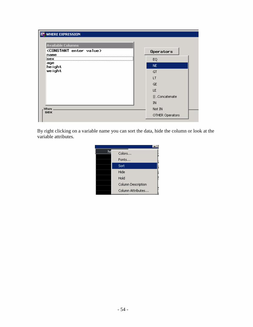
- 54 -

By right clicking on a variable name you can sort the data, hide the column or look at the

variable attributes.

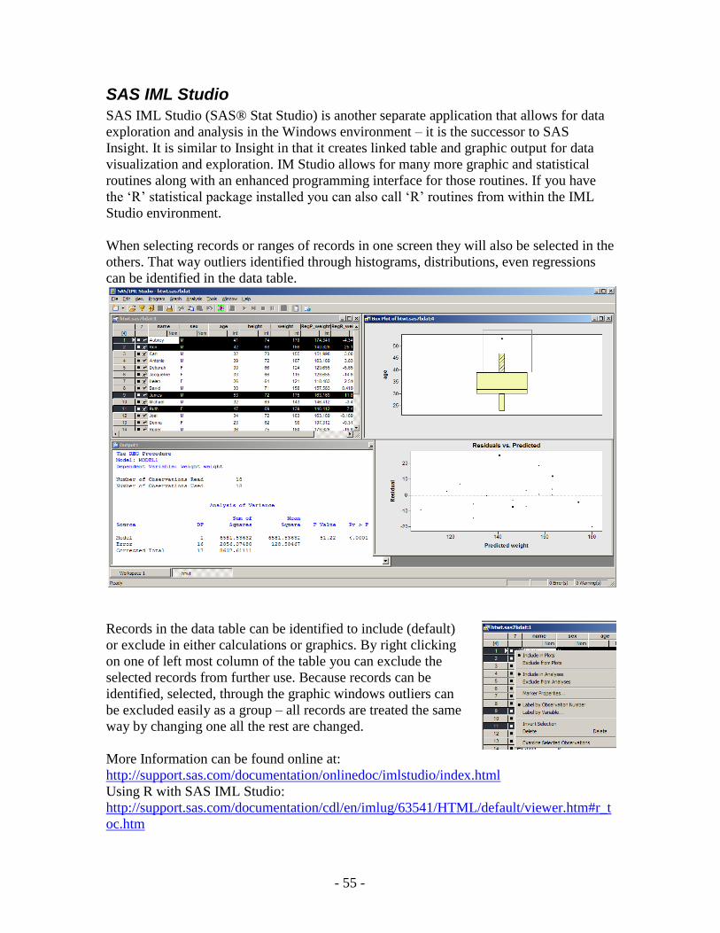
- 55 -

SAS IML Studio

SAS IML Studio (SAS® Stat Studio) is another separate application that allows for data

exploration and analysis in the Windows environment – it is the successor to SAS

Insight. It is similar to Insight in that it creates linked table and graphic output for data

visualization and exploration. IM Studio allows for many more graphic and statistical

routines along with an enhanced programming interface for those routines. If you have

the ‘R’ statistical package installed you can also call ‘R’ routines from within the IML

Studio environment.

When selecting records or ranges of records in one screen they will also be selected in the

others. That way outliers identified through histograms, distributions, even regressions

can be identified in the data table.

Records in the data table can be identified to include (default)

or exclude in either calculations or graphics. By right clicking

on one of left most column of the table you can exclude the

selected records from further use. Because records can be

identified, selected, through the graphic windows outliers can

be excluded easily as a group – all records are treated the same

way by changing one all the rest are changed.

More Information can be found online at:

http://support.sas.com/documentation/onlinedoc/imlstudio/index.html

Using R with SAS IML Studio:

http://support.sas.com/documentation/cdl/en/imlug/63541/HTML/default/viewer.htm#r_t

oc.htm

- 56 -

SAS Enterprise Guide

Starting with SAS 9.2 SAS Enterprise Guide is available under the University site

licence. What is SAS EG you might ask? SAS Enterprise Guide is a separate SAS

application that provides a graphic interface to SAS data manipulation and analysis –

basically it writes SAS code for you using a visual programming environment, or

Designer, where you just need to select data and tasks through menu items or dialog

boxes. Tasks are displayed as interconnected icons in the Designer following a Process

Flow. The tasks and programs in a process flow can all be saved in a Project. Projects

then can be opened again and re-run as a whole unit, process branches, or even individual

tasks. Each task can be opened and the actual code, log, and results previewed. Your own

SAS code can be added allowing you to use both the pre-set tasks and user defined

programs. The code from the GUI created tasks can be copied into your own code for

modification if necessary. An existing SAS program can even be analyzed and converted

into a process flow. Enterprise Guide is now the default environment that is opened under

Windows when a SAS dataset or program is opened from Windows Explorer.

This introduction to EG is very brief additional documentation can be found from the

SAS online documentation. There are a number of very helpful third party online

references – because EG is changing rapidly you may be better off doing an internet

search. I have found The Little SAS Book for Enterprise Guide® by Susan Slaughter and

Lora Delwiche a helpful introduction.

Enterprise Guide Environment

Like many Windows based programs today the Enterprise Guide environment can be

highly modified with multiple docking windows and screens.

If you have re-arranged the windows (on purpose or by

accident) and want to return to the default settings just select

‘Restore Window Layout’ under the General tab under Tools->Options menu.

The work that you do in Enterprise Guide can be saved into projects where a Project is a

collection of related tasks and contains all of the pointers to existing data (but not the

data), tasks, code, results, and logs. Complex projects can be broken, or displayed, as

- 57 -

several process flows. Just like your regular SAS code the data is not actually stored as

part of the project so it can be used in many places within the same or other projects.

Although projects can be saved as a separate file, and given to other people, remember

that it does not contain the actual data or linked code and the final users must have the

ability to create the same library or file access or the Project (and contained processes &

tasks) will not run.

A Project contains a number of icons (nodes) that follow a specific process flow. The

design of the process and associated tasks are done within the Project Designer window

or Explorer. The Project Designer can have several types of items:

Data: Represent SAS datasets in either permanent or temporary libraries, raw data files

or tables from other database applications (e.g. Excel or MS Access). These are just

pointers to the external data files (note the little arrow on the bottom left).

Tasks: Specific data manipulation or analysis requests. This can be a simple query to a

complex statistical analysis request or even a SAS program that you have written. Tasks,

in particular program code, that is linked to an external file will contain a small arrow on

the bottom left side of the task icon.

Most tasks are associated with one or more SAS procedures. SAS has provided a list of

tasks and the corresponding procedure that is used/required:

http://support.sas.com/documentation/onlinedoc/guide/sastasksandprocs.htm

Results: Resulting tables, reports, or graphs or other output that are created by Tasks.

Notes: Generally these are used for documentation or commenting on your project.

- 58 -

Define SAS Library

If you want to create your own library as part of the process select Assign Project

Library… from under the tools menu. This step is not always necessary, but good

practise, as Enterprise Guide will generate a library for you as part of the project.

Once a library is generated you might want to include it as part of your process flow.

Adding it to the process flow through a link will allow you to include it when re-running

parts of your project.

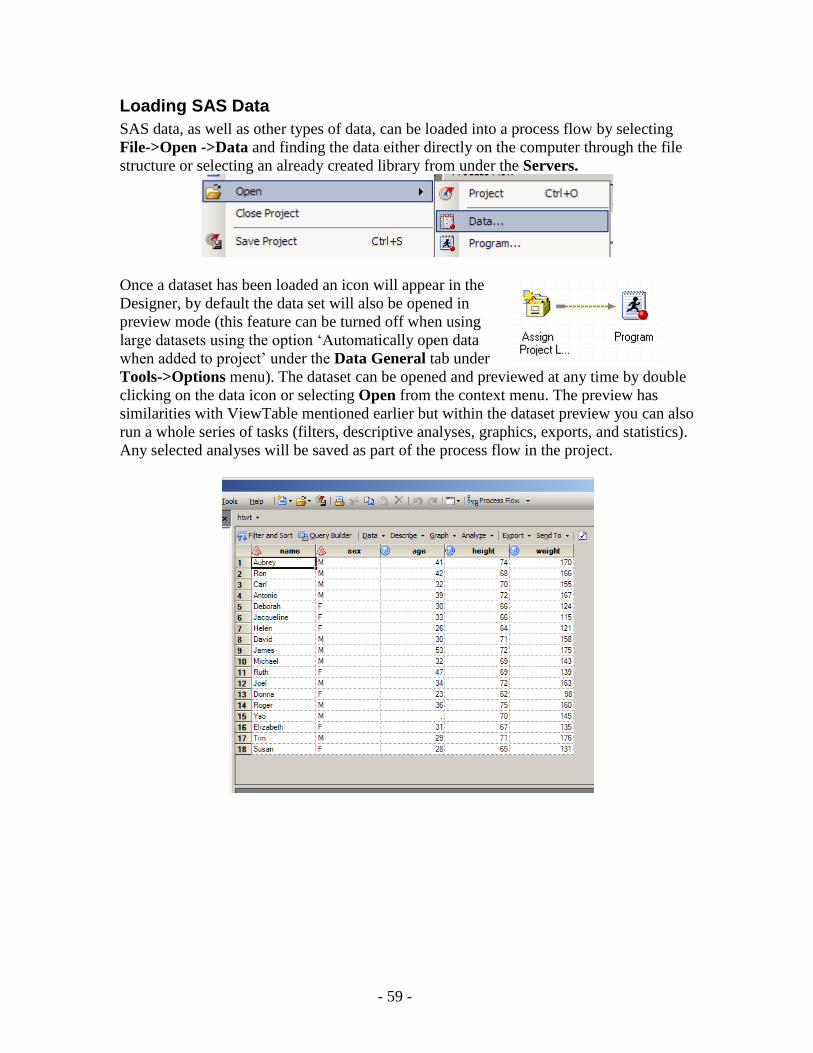
- 59 -

Loading SAS Data

SAS data, as well as other types of data, can be loaded into a process flow by selecting

File->Open ->Data and finding the data either directly on the computer through the file

structure or selecting an already created library from under the Servers.

Once a dataset has been loaded an icon will appear in the

Designer, by default the data set will also be opened in

preview mode (this feature can be turned off when using

large datasets using the option ‘Automatically open data

when added to project’ under the Data General tab under

Tools->Options menu). The dataset can be opened and previewed at any time by double

clicking on the data icon or selecting Open from the context menu. The preview has

similarities with ViewTable mentioned earlier but within the dataset preview you can also

run a whole series of tasks (filters, descriptive analyses, graphics, exports, and statistics).

Any selected analyses will be saved as part of the process flow in the project.

- 60 -

Data Manipulation – sort, merge, concatenation, formats

All of the basic data step and data manipulation

processes can be done through the graphic

interface using one of the options under Tasks-

>Data->. The Query Builder is probably the most

powerful of these tools as it will allow you to

graphically build SQL statements.

Once a data manipulation task has been selected

an icon is added to the designer within the process

flow.

Some data manipulation tasks are obvious others

are a little more obscure for people already

familiar with base SAS programming.

- Creating/calculating new variables is done

through the Query Builder.

- Concatenating (setting) multiple datasets

together is done with Append.

- Merging data is done with the Query Builder using a Join.

- Sub-setting data is done using Filter and Sort or Query Builder.

Data sets can be opened, viewed and edited directly in a ‘Data Grid’ by

double clicking on a data item or selecting Open from the pop-up

menu. The Data Grid view of data will give you access to most analytic

and data tasks as well as allowing you to directly manipulate data

values, columns and rows. By default data sets are “locked” in a

protected mode so the underlying data can not accidentally be changed.

If you wish to edit the data un-select the Protect Data option under the

Edit menu.

Important Note Editing data interactively in the

Data Grid, including adding

columns or rows, does not write

any SAS code or generate log

entries. This means that any

changes made will not be

replicated when the project or

process flow is re-run.

- 61 -

Analysis, Options, and SAS code

At any point you can select an analytic task to add to your

project. The default data used is the currently active

(selected) data in your process flow.

Each task that is select provides a series of options that

are appropriate for that task. In this case the Summary

Statistics task has been selected. Once you are finished

selecting the options you are interested in using the task

can be run immediately or it can be saved to the project

for running later.

On the left side of the dialog box you can select the data

to use, type of analysis, additional options. Depending on

what is selected on the left different options will be displayed in the middle of the screen.

When you are finished you can run the task (this also saves it in the process flow), save

as part of the process, or preview the code (and copy if necessary).

Once the task has been run the results are displayed including access to the SAS log, the

code that Enterprise Guide created, Access to the original task and data, and options to

save the output in various formats.

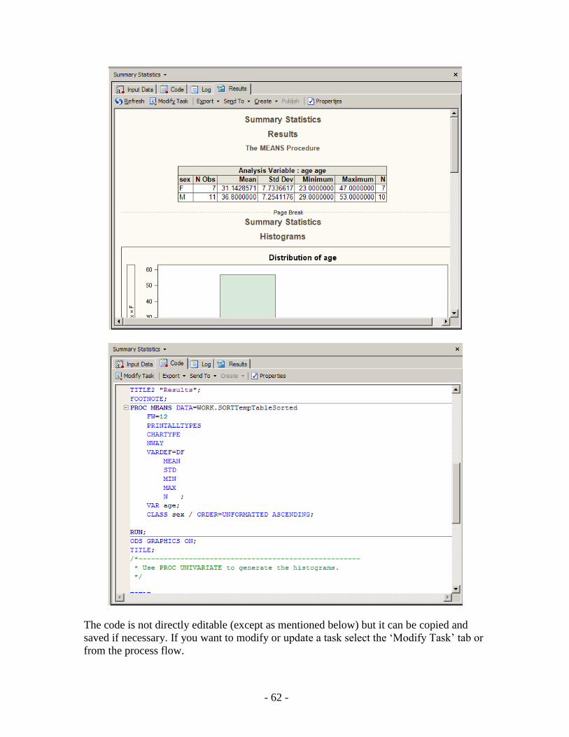
- 62 -

The code is not directly editable (except as mentioned below) but it can be copied and

saved if necessary. If you want to modify or update a task select the ‘Modify Task’ tab or

from the process flow.

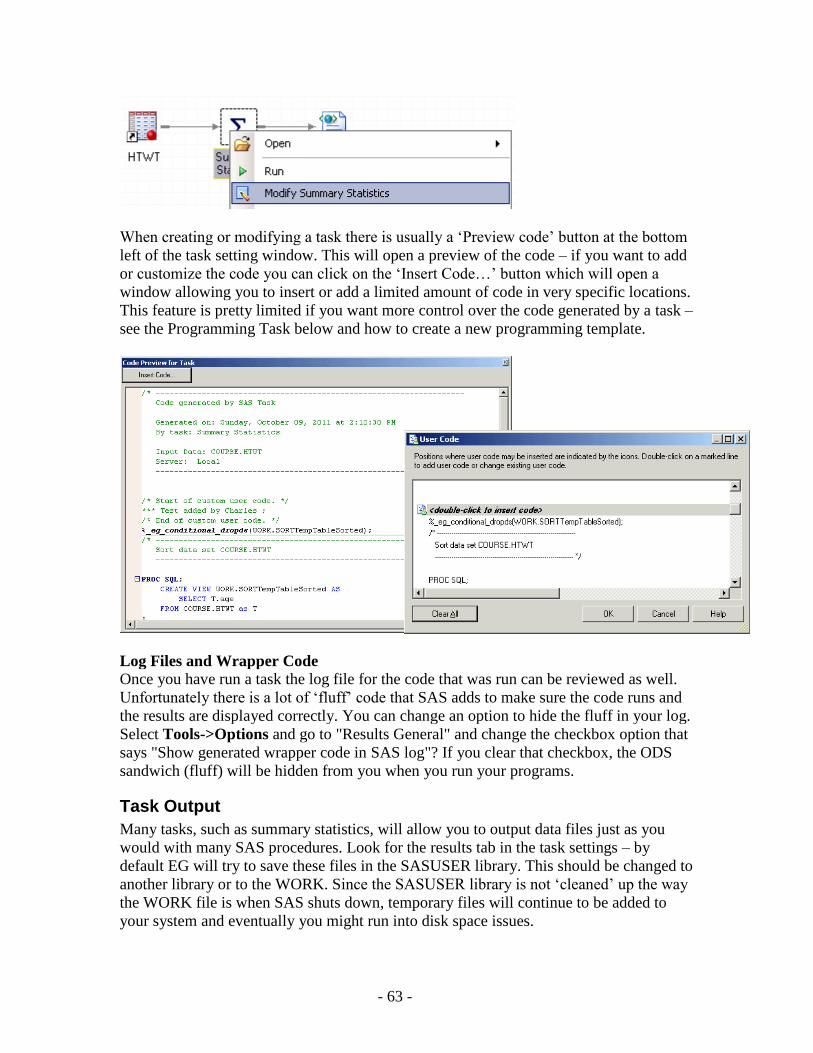
- 63 -

When creating or modifying a task there is usually a ‘Preview code’ button at the bottom

left of the task setting window. This will open a preview of the code – if you want to add

or customize the code you can click on the ‘Insert Code…’ button which will open a

window allowing you to insert or add a limited amount of code in very specific locations.

This feature is pretty limited if you want more control over the code generated by a task –

see the Programming Task below and how to create a new programming template.

Log Files and Wrapper Code

Once you have run a task the log file for the code that was run can be reviewed as well.

Unfortunately there is a lot of ‘fluff’ code that SAS adds to make sure the code runs and

the results are displayed correctly. You can change an option to hide the fluff in your log.

Select Tools->Options and go to "Results General" and change the checkbox option that

says "Show generated wrapper code in SAS log"? If you clear that checkbox, the ODS

sandwich (fluff) will be hidden from you when you run your programs.

Task Output

Many tasks, such as summary statistics, will allow you to output data files just as you

would with many SAS procedures. Look for the results tab in the task settings – by

default EG will try to save these files in the SASUSER library. This should be changed to

another library or to the WORK. Since the SASUSER library is not ‘cleaned’ up the way

the WORK file is when SAS shuts down, temporary files will continue to be added to

your system and eventually you might run into disk space issues.

- 64 -

The default can be changed by selecting WORK using the Output Library option under

Tools->Options. This also changes the order that EG searches for files, that may have the

same name, so you may need to be careful about the order, libraries and what is being

saved into each library or you might get some unexpected output.

Customized result format and output

Using the Results options found under Tasks->Options you can change the format of the

output from individuals tasks. These options can also be ‘tweaked’ within each task or

program node individually by editing the Results property through the Property item on

the task sensitive menu.

The output format can be saved as normal SAS reports (text that is) but also written into

RTF, HTML, PDF format. If you have a particular viewer (e.g. MS Word) that you

would like to use the viewer can be identified.

Using your Own Code

Access to some options, procedures, or complex data processing steps is not possible

through the Enterprise Guide interface. In particular doing iterative (do loop or array)

processing and by group processing is difficult in a graphic environment. Setting up

formats is possible through the graphic interface but it can be slow for programmers

familiar using PROC FORMAT. It is still possible to write SAS programming through

program tasks or nodes allowing users to write and use more complex processing tasks.

- 65 -

To create a new program node select ‘New Program’ from under the File or Program

menu, or open an existing SAS program. In either case a program node, which can be

renamed, will be added to your designer window and a SAS code editor will be opened.

The Enterprise Guide program editor has the same functionality as the display manager

editor but it also includes some additional capabilities. You can write and submit code as

you normally would in SAS.

If you want to tweak code that has been created by a SAS EG task you can select ‘Add

code as Template from the pop-up menu for any task in the designer. This will create a

new program node with the code generated by EG. If you try to edit generated code

within a task you will also be asked if you want to create an editable copy of the code.

or

When creating code this way the wrapper code (fluff) mentioned above is still copied

over to the new program code. Along with the wrapper code in many tasks a lot of extra

code is added (e.g. extra sort or data steps) that can be avoided if you are comfortable

with writing your own code and controlling the flow of the data. This extra code is added

by SAS to ensure your data is not destroyed and to make sure that the data is in the

necessary format for the identified procedure (task).

Because EG sometimes uses unfamiliar library names, esptically if you load data from

the file manager, it can be difficult to work out what library and dataset name to use in a

programming task. By opening a program node and draging a database from the Project

Tree into the editor SAS writes the database name, and library if necessary, as a comment

in the code. This can be modified as necessary for set/merge statements or used in a data=

option on a procedure.

/*** Data dragged from Project Tree when opened from File Manage **/

LIBNAME ECLIB000 "X:\course\Data";

/*Data Source: ECLIB000.htwt */

/*** Data dragged from Project Tree when opened from Library **/

/*Data Source: WORK.TEST */

- 66 -

When the program is run any created data sets and results are shown as linked results or

data items. Programs can be added into the process flow by selecting ‘Link ___ to…’

from the pop-up menu.

If you open an external SAS program from the File or Program menu the code is linked

back to the original and not actually stored as part of the project. If you want to include or

embed the code right into the project (like a program task created in the project) open the

program properties

Tool Tips and Interactive Help

The Starting with Enterprise Guide 4.3 (and SAS 9.3) the SAS editor has many

interactive tools to assist the programmer. Although

you still have to type out the code, the new tools will

make reduce the number of typographic and syntax

errors.

SAS will provide options to auto-complete words,

options, datasets, procedures based on the locatoin of

the cursor in the program and the first two letters

typed of each word. This includes procedures,

accepted options, and even available data sets or

macro variables. This feature is turned on by default

- 67 -

but it can be controlled under the Program Menu->Editor Options… using the

Autocomplete tab.

The program editor highlights matching parentheses pairs as you navigate – this helps

ensure that all of your brackets/parenthises are balanced appropriately. You can also use

the Ctrl+[ (open bracket) key to move the cursor from one parenthesis to its match. If no

match can be found the program editor just beeps.

By hovering over a SAS recognized word (blue or dark blue) in the program editor all of

the syntax options and associated help are displayed in a pop-up window. This option is

very helpful when trying to understand or determine the syntax required for a particular

command or statement.

SAS can format your code in a consistent and structored fashion. Although it will not

correct your code it will make it easier to read and find errors. In the program editor

select Format Code under the a context (right click) menu or Edit->Format Code, or

press Ctrl+I.

If the code can not be formatted for some reason, SAS will return a message that

indicates the problem (if it can be determined) and the location.

Formatting Error Please check for an unmatched parenthesis on line 100

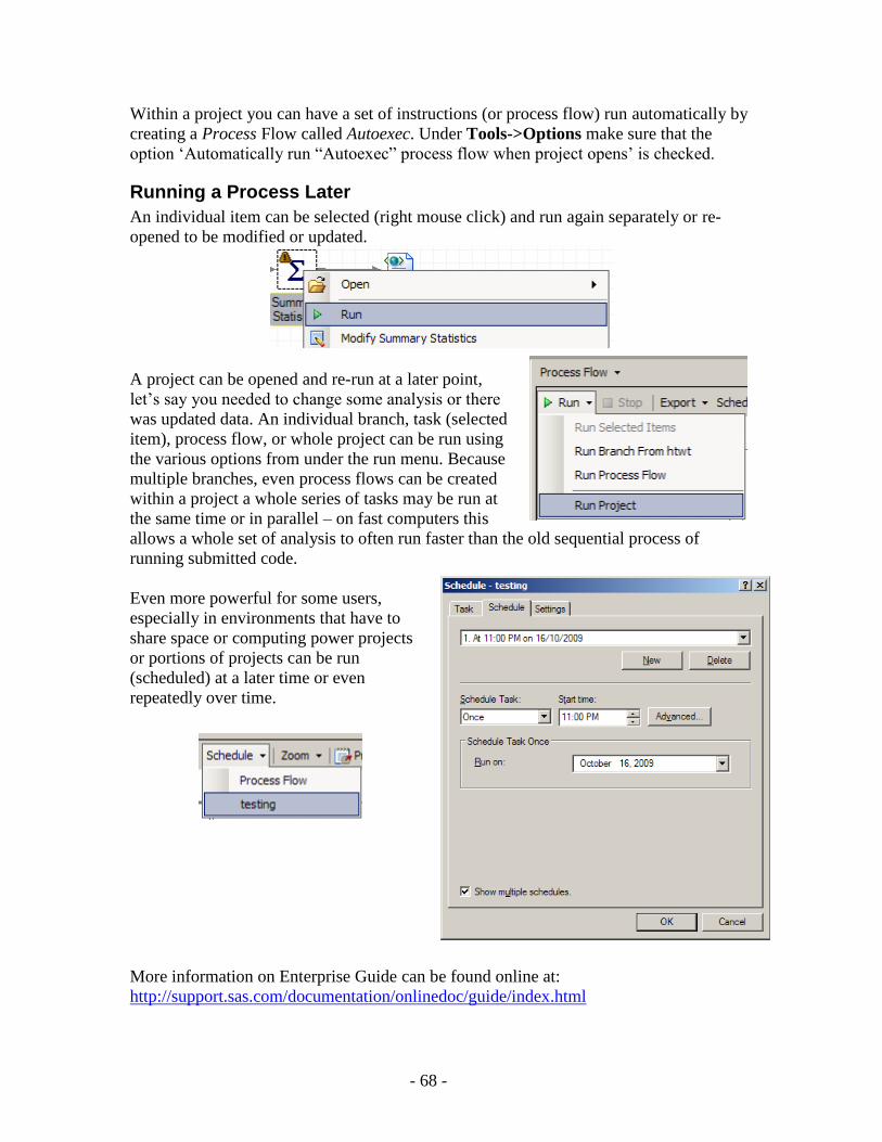
- 68 -

Within a project you can have a set of instructions (or process flow) run automatically by

creating a Process Flow called Autoexec. Under Tools->Options make sure that the

option ‘Automatically run “Autoexec” process flow when project opens’ is checked.

Running a Process Later

An individual item can be selected (right mouse click) and run again separately or re-

opened to be modified or updated.

A project can be opened and re-run at a later point,

let’s say you needed to change some analysis or there

was updated data. An individual branch, task (selected

item), process flow, or whole project can be run using

the various options from under the run menu. Because

multiple branches, even process flows can be created

within a project a whole series of tasks may be run at

the same time or in parallel – on fast computers this

allows a whole set of analysis to often run faster than the old sequential process of

running submitted code.

Even more powerful for some users,

especially in environments that have to

share space or computing power projects

or portions of projects can be run

(scheduled) at a later time or even

repeatedly over time.

More information on Enterprise Guide can be found online at:

http://support.sas.com/documentation/onlinedoc/guide/index.html

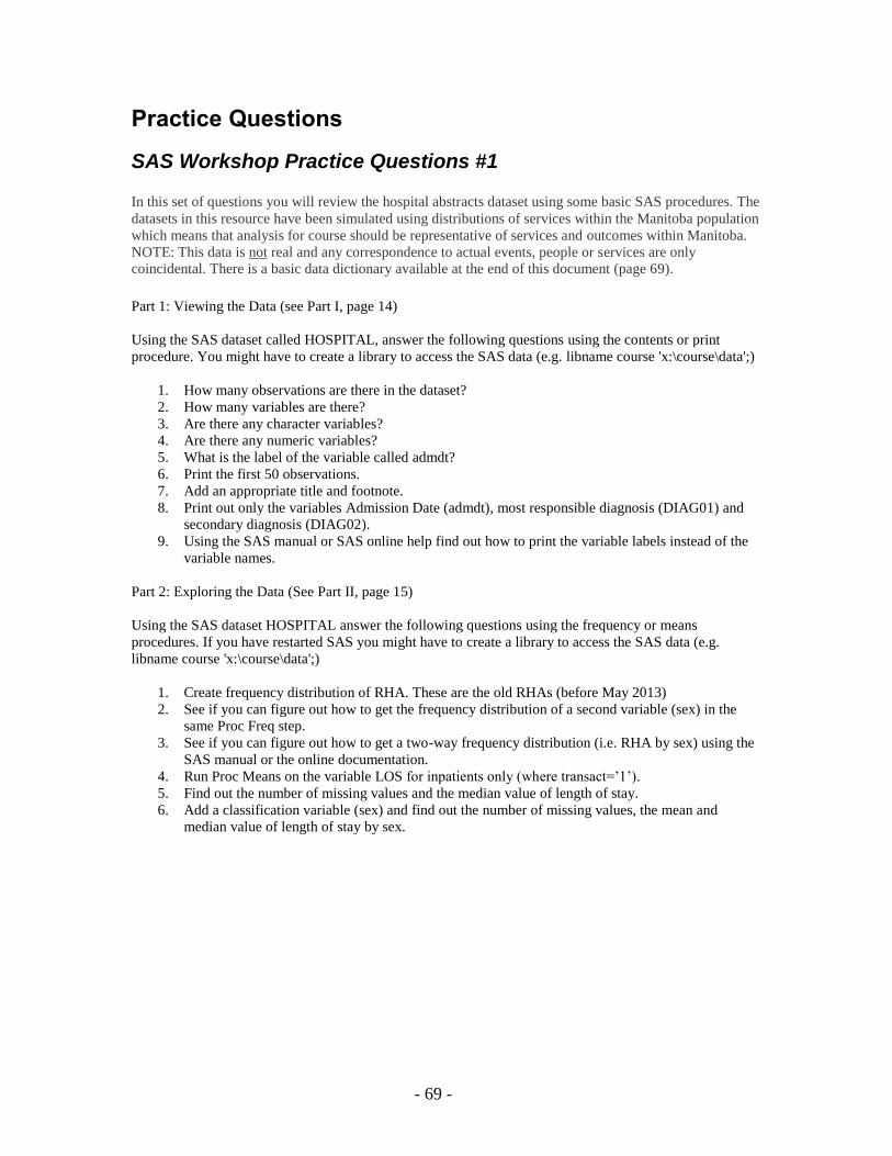
- 69 -

Practice Questions

SAS Workshop Practice Questions #1

In this set of questions you will review the hospital abstracts dataset using some basic SAS procedures. The

datasets in this resource have been simulated using distributions of services within the Manitoba population

which means that analysis for course should be representative of services and outcomes within Manitoba.

NOTE: This data is not real and any correspondence to actual events, people or services are only

coincidental. There is a basic data dictionary available at the end of this document (page 69).

Part 1: Viewing the Data (see Part I, page 14)

Using the SAS dataset called HOSPITAL, answer the following questions using the contents or print

procedure. You might have to create a library to access the SAS data (e.g. libname course 'x:\course\data';)

1. How many observations are there in the dataset?

2. How many variables are there?

3. Are there any character variables?

4. Are there any numeric variables?

5. What is the label of the variable called admdt?

6. Print the first 50 observations.

7. Add an appropriate title and footnote.

8. Print out only the variables Admission Date (admdt), most responsible diagnosis (DIAG01) and

secondary diagnosis (DIAG02).

9. Using the SAS manual or SAS online help find out how to print the variable labels instead of the

variable names.

Part 2: Exploring the Data (See Part II, page 15)

Using the SAS dataset HOSPITAL answer the following questions using the frequency or means

procedures. If you have restarted SAS you might have to create a library to access the SAS data (e.g.

libname course 'x:\course\data';)

1. Create frequency distribution of RHA. These are the old RHAs (before May 2013)

2. See if you can figure out how to get the frequency distribution of a second variable (sex) in the

same Proc Freq step.

3. See if you can figure out how to get a two-way frequency distribution (i.e. RHA by sex) using the

SAS manual or the online documentation.

4. Run Proc Means on the variable LOS for inpatients only (where transact=’1’).

5. Find out the number of missing values and the median value of length of stay.

6. Add a classification variable (sex) and find out the number of missing values, the mean and

median value of length of stay by sex.

- 70 -

SAS Workshop Practice Questions #2 In this practice session you will import raw (ASCII) data and create new variables. If you have just started

a new SAS session remember to define a SAS library.

Part 1: Reading Raw Data into a Temporary SAS dataset

A. Look at the format of the raw data file – x:\course\Raw Data\hospital07.txt. You

can open this file in the SAS program editor or the Windows Notepad application.

i. How is the data arranged?

ii. Clear this file from the window by using pull-down menu Edit and clicking clear all.

B. Open up SAS program – x:\course\Formats\newfmts 2012.sas. This file contains a

list of formats that can be used with the HOSPITAL data.

i. How does this set of proc format statements compare to what you learned on page 18?

ii. Run newfmts.sas and look at the SAS log.

iii. Clear this file from the window.

iv. In the future you can include (or run) this program without opening it in the program

editor using the following SAS statement:

%include ‘x:\course\Formats\newfmts 2012.sas’; C. In a data step, use an infile followed by an input statement to create a new SAS dataset from the

raw ASCII hospital data.

i. Use an ‘infile’ statement similar to the one on page 19 to access the data.

Infile ‘x:\course\Raw Data\hospital07.txt’; ii. The following table provides the location and labels for variables in the raw data. Use this

information with an input statement to read the data. Remember that variable names

should be a single word and short (e.g. the variable name for age at admission could be

ageadm). Character variables are identified using a $ on the input statement.

Variable Name Label Type Start Column End Column Format

Sex Sex Char 10 10 $sexL.

Ageadm Age at admission Num 19 22

Los Length of Stay (LOS) Num 43 46

Area Region of Residence Char 23 23 $areaL.

D. Create labels for each of the variables you were read into the dataset.

E. Format gender and region of residence with the correct format (provided in the file newfmts.sas).

F. Calculate the mean and median value of length of stay by sex (see page 15).

Part 2: Manipulating Data

In this example you will create new datasets and do some basic analysis using the SAS HOSPITAL data

found in X:\course\data. (remember to use a SAS library to access SAS datasets). Using the HOSPITAL

data in course uses a different set of formats - %include ‘x:\course\Formats\newfmts.sas’;

A. Create two new temporary SAS datasets (INPAT, DAYSURG) from COURSE.HOSPITAL in a

single data step keeping only the variables sex, and length of stay (e.g. page 20).

i. INPAT data should contain observations from HOSPITAL with TRANSACT equal to1.

ii. DAYSURG data should contain observations from HOSPTIAL with TRANSACT equal

3.

iii. Calculate the mean length of stay (LOS) for INPAT and DAYSURG hospital separations.

Remember to use titles to identify your output appropriately (page 15). Day Surgery

records are recorded in hours.

B. Using the dataset COURSE.HOSPITAL, calculate the frequency distribution of sex for INPAT

and DAYSURG using a where statement (see page 21).

C. In a temporary (WORK) copy of the Inpatient HOSPITAL dataset, create the following new

variables:

- 71 -

i. Create an AGE variable using the following calculation. We will cover SAS date values

later in the course. AGE = floor( (ADMDT-BIRTHDT)/365.25) ;

ii. Create an agegroup variable which groups age into 4 categories (see page 22)

0-19, 20-39, 40-59, 60 or more

iii. Label the age group variable and create a format to label the values of the age group

variable. Remember that a SAS format must be created in a separate step using proc

format before it is used.

iv. Create a short_stay indicator variable that indicates the records where the length of stay

is less than 3. Label this variable appropriately.

v. Using the new variables calculate the proportion of hospital stays with length of stay less

than 3 days by age group (see proc means page 22).

- 72 -

SAS Workshop Practice Questions #3

In this example you will use the simulated hospital abstract data to determine the number

of inpatient (TRANSACT=’1’) cases in three geographic groups that stay longer than the

average length of stay for that group.

A. Create a temporary copy of the permanent COURSE.HOSPTIAL dataset, to do

the following. This can be done in a data step setting the hospital data from a

defined library.

B. Create a variable which groups the rha variable into 3 groups using a format or

if/then conditional processing.

Group RHA

North ‘NO’ Northern

South ‘SO’ Southern

‘IE’ Interlake-Eastern

‘WE’ Prairie Mountain

Urban ‘WP’ Winnipeg

Include the formats for this data using %include ‘X:\course\formats\newfmts.sas’ ;

C. Calculate the average length of stay by area group and sex using proc means.

Output the results into a temporary SAS (see page 28)

D. Merge the average length of stay variable to the temporary HOSPITAL dataset by

the area group and sex (see page 28)

E. Create a new variable that indicates whether the length of stay for the case is

greater than the group specific average length of stay. Label this variable

appropriately (see high_age example page 29).

F. Report the number of cases and the proportion of cases that have a length of stay

greater than the average length of stay by sex and area group using proc means.

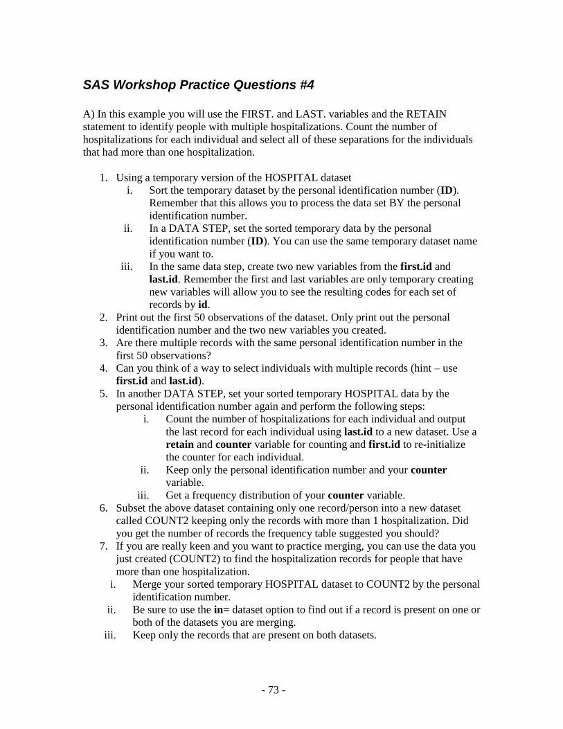
- 73 -

SAS Workshop Practice Questions #4

A) In this example you will use the FIRST. and LAST. variables and the RETAIN

statement to identify people with multiple hospitalizations. Count the number of

hospitalizations for each individual and select all of these separations for the individuals

that had more than one hospitalization.

1. Using a temporary version of the HOSPITAL dataset

i. Sort the temporary dataset by the personal identification number (ID).

Remember that this allows you to process the data set BY the personal

identification number.

ii. In a DATA STEP, set the sorted temporary data by the personal

identification number (ID). You can use the same temporary dataset name

if you want to.

iii. In the same data step, create two new variables from the first.id and

last.id. Remember the first and last variables are only temporary creating

new variables will allow you to see the resulting codes for each set of

records by id.

2. Print out the first 50 observations of the dataset. Only print out the personal

identification number and the two new variables you created.

3. Are there multiple records with the same personal identification number in the

first 50 observations?

4. Can you think of a way to select individuals with multiple records (hint – use

first.id and last.id).

5. In another DATA STEP, set your sorted temporary HOSPITAL data by the

personal identification number again and perform the following steps:

i. Count the number of hospitalizations for each individual and output

the last record for each individual using last.id to a new dataset. Use a

retain and counter variable for counting and first.id to re-initialize

the counter for each individual.

ii. Keep only the personal identification number and your counter

variable.

iii. Get a frequency distribution of your counter variable.

6. Subset the above dataset containing only one record/person into a new dataset

called COUNT2 keeping only the records with more than 1 hospitalization. Did

you get the number of records the frequency table suggested you should?

7. If you are really keen and you want to practice merging, you can use the data you

just created (COUNT2) to find the hospitalization records for people that have

more than one hospitalization.

i. Merge your sorted temporary HOSPITAL dataset to COUNT2 by the personal

identification number.

ii. Be sure to use the in= dataset option to find out if a record is present on one or

both of the datasets you are merging.

iii. Keep only the records that are present on both datasets.

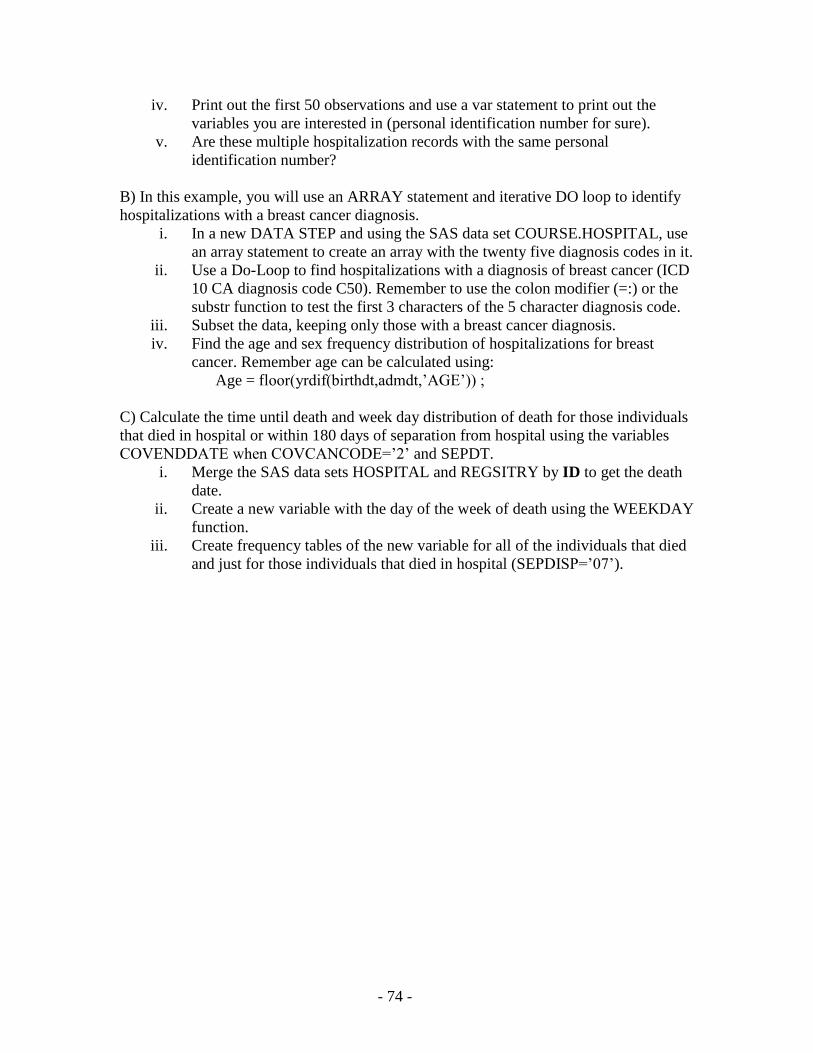
- 74 -

iv. Print out the first 50 observations and use a var statement to print out the

variables you are interested in (personal identification number for sure).

v. Are these multiple hospitalization records with the same personal

identification number?

B) In this example, you will use an ARRAY statement and iterative DO loop to identify

hospitalizations with a breast cancer diagnosis.

i. In a new DATA STEP and using the SAS data set COURSE.HOSPITAL, use

an array statement to create an array with the twenty five diagnosis codes in it.

ii. Use a Do-Loop to find hospitalizations with a diagnosis of breast cancer (ICD

10 CA diagnosis code C50). Remember to use the colon modifier (=:) or the

substr function to test the first 3 characters of the 5 character diagnosis code.

iii. Subset the data, keeping only those with a breast cancer diagnosis.

iv. Find the age and sex frequency distribution of hospitalizations for breast

cancer. Remember age can be calculated using:

Age = floor(yrdif(birthdt,admdt,’AGE’)) ;

C) Calculate the time until death and week day distribution of death for those individuals

that died in hospital or within 180 days of separation from hospital using the variables

COVENDDATE when COVCANCODE=’2’ and SEPDT.

i. Merge the SAS data sets HOSPITAL and REGSITRY by ID to get the death

date.

ii. Create a new variable with the day of the week of death using the WEEKDAY

function.

iii. Create frequency tables of the new variable for all of the individuals that died

and just for those individuals that died in hospital (SEPDISP=’07’).

- 75 -

SAS Workshop Practice Questions #5

Using the hospital and registry data calculate the crude rates for 2009 of inpatient hospital

separations, total days, and individuals by region.

Hint:

You will need to summarize the registry by region by creating a temporary data

set with a population variable. Select the registry data so there is only a single

record/person (ID). The registry data includes individuals that may have been

born or died during the time period. You may want to select a ‘census’ population

for a particular time period (e.g. mid time period).

You will need to summarize the hospital data by region. Remember the hospital

data contains data for several years of data.

Merge this summarized data.

- 76 -

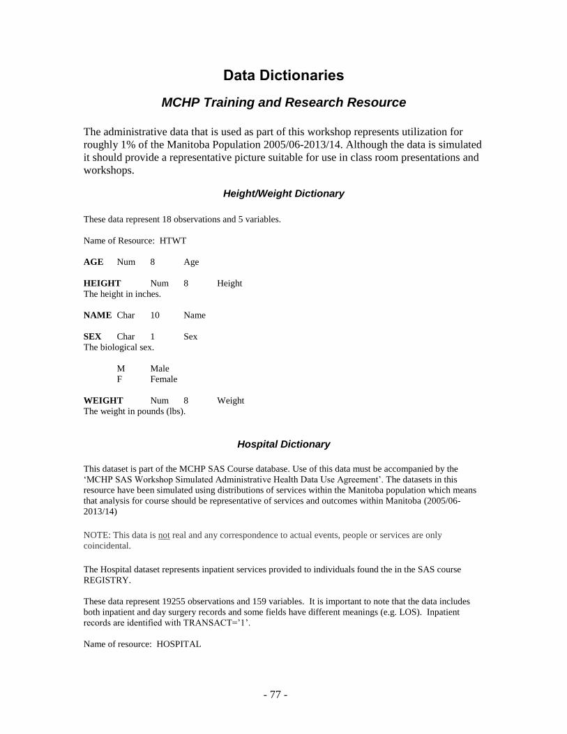
- 77 -

Data Dictionaries

MCHP Training and Research Resource

The administrative data that is used as part of this workshop represents utilization for

roughly 1% of the Manitoba Population 2005/06-2013/14. Although the data is simulated

it should provide a representative picture suitable for use in class room presentations and

workshops.

Height/Weight Dictionary

These data represent 18 observations and 5 variables.

Name of Resource: HTWT

AGE Num 8 Age

HEIGHT Num 8 Height

The height in inches.

NAME Char 10 Name

SEX Char 1 Sex

The biological sex.

M Male

F Female

WEIGHT Num 8 Weight

The weight in pounds (lbs).

Hospital Dictionary

This dataset is part of the MCHP SAS Course database. Use of this data must be accompanied by the

‘MCHP SAS Workshop Simulated Administrative Health Data Use Agreement’. The datasets in this

resource have been simulated using distributions of services within the Manitoba population which means

that analysis for course should be representative of services and outcomes within Manitoba (2005/06-

2013/14)

NOTE: This data is not real and any correspondence to actual events, people or services are only

coincidental.

The Hospital dataset represents inpatient services provided to individuals found the in the SAS course

REGISTRY.

These data represent 19255 observations and 159 variables. It is important to note that the data includes

both inpatient and day surgery records and some fields have different meanings (e.g. LOS). Inpatient

records are identified with TRANSACT=’1’.

Name of resource: HOSPITAL

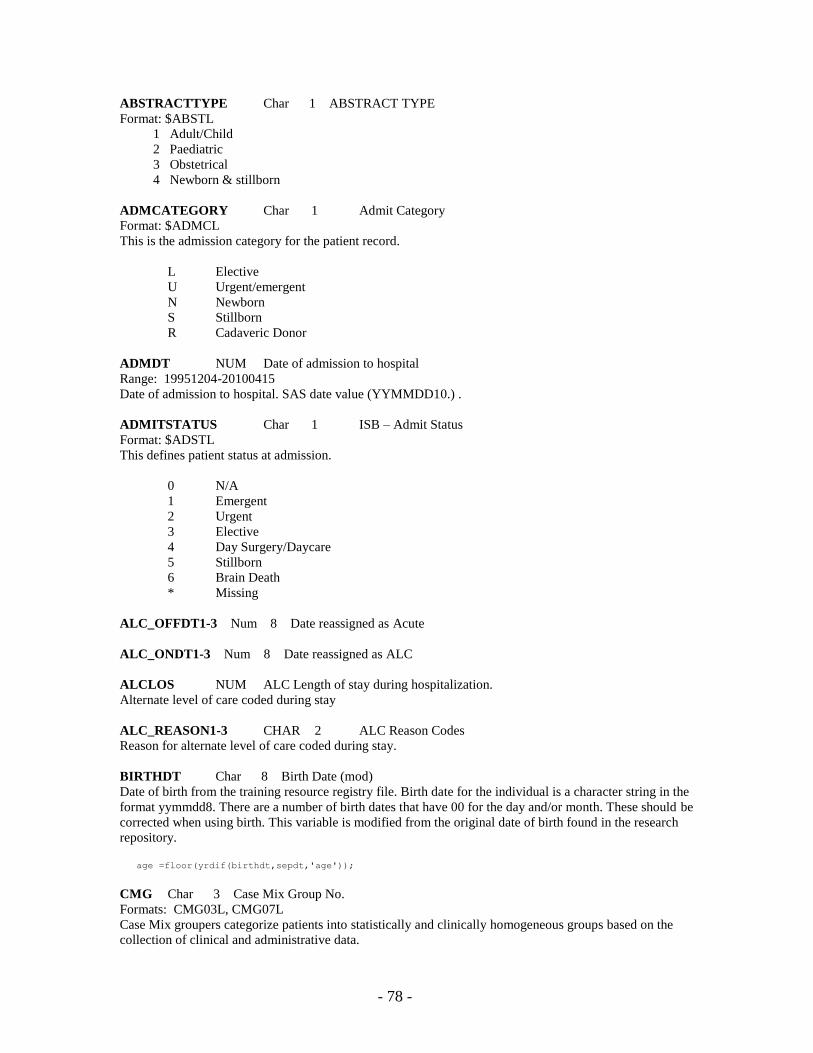
- 78 -

ABSTRACTTYPE Char 1 ABSTRACT TYPE

Format: $ABSTL

1 Adult/Child

2 Paediatric

3 Obstetrical

4 Newborn & stillborn

ADMCATEGORY Char 1 Admit Category

Format: $ADMCL

This is the admission category for the patient record.

L Elective

U Urgent/emergent

N Newborn

S Stillborn

R Cadaveric Donor

ADMDT NUM Date of admission to hospital

Range: 19951204-20100415

Date of admission to hospital. SAS date value (YYMMDD10.) .

ADMITSTATUS Char 1 ISB – Admit Status

Format: $ADSTL

This defines patient status at admission.

0 N/A

1 Emergent

2 Urgent

3 Elective

4 Day Surgery/Daycare

5 Stillborn

6 Brain Death

* Missing

ALC_OFFDT1-3 Num 8 Date reassigned as Acute

ALC_ONDT1-3 Num 8 Date reassigned as ALC

ALCLOS NUM ALC Length of stay during hospitalization.

Alternate level of care coded during stay

ALC_REASON1-3 CHAR 2 ALC Reason Codes

Reason for alternate level of care coded during stay.

BIRTHDT Char 8 Birth Date (mod)

Date of birth from the training resource registry file. Birth date for the individual is a character string in the

format yymmdd8. There are a number of birth dates that have 00 for the day and/or month. These should be

corrected when using birth. This variable is modified from the original date of birth found in the research

repository.

age =floor(yrdif(birthdt,sepdt,'age'));

CMG Char 3 Case Mix Group No.

Formats: CMG03L, CMG07L

Case Mix groupers categorize patients into statistically and clinically homogeneous groups based on the

collection of clinical and administrative data.

- 79 -

DIAG01-25 Char 7 ICD-10-CA Diagnosis Code

DPG4 Char 2 Day Procedure Group

Formats: $DPG03L, $DPG06L, $DPG07L

This is a national grouping methodology for ambulatory hospital patients mainly in the area of day surgery.

Note that patients are assigned to categories according to the principal (most significant) procedure

recorded on the patient abstract. Patients assigned to the same DPG category represent a homogeneous

group with similar clinical episodes and requiring similar resources.

DPGRIW Num 8 Day Procedure Group Weight

Range: 0.015-4.4586

A relative resource allocation methodology for estimating a hospital’s day procedure costs, based on the

same scale as the inpatient RIW

HOSPRHA Char 2 RHA of Hospital

Format: $RHAL

This is the RHA location of the Hospital. See RHA for codes.

ID Char 6 Personal ID Number (Mod)

This is a personal identifier that can be used in all of the training resource data. It is NOT related to PHIN

or family registration number. For more information on individuals, refer to CENSUS2001, REGISTRY, or

REGISTRY_FAMILY.

INTCD01-20 Char 10 CCI Intervention Code

The intervention code is an operative or non-operative intervention performed during the patient’s hospital

stay. The CCI does not provide a code to classify an intervention that did not occur.

Column Field

1 Section

2-3 Group Anatomy, Stage, Group, Functional, or Type. Depending on section

4-5 Intervention

6-7 Approach, Technique, Reason. Depending on section

8-9 Device, Agent, Method used

10 Tissue

CCI Rubric Formats

The following formats can be used to format the individual rubrics within each CCI.

Field 1 Field 2 Field 3 Field 4 Field 5 Field 6

Section

Group Anatomy, Stage,

Group, Functional,

Type)

Intervention

Approach

Technique,

reason

Device, agent,

method used

Tissue

Used

1 digit 2 digit 2 digits 2 digits 2 digits 1 digit

Format Name

$CCISECL $GrpS123l $S1_Int $Q1S1l $Q2S1l $Q3S1l

$CCISECL $GrpS123l $S2_Int $Q1S2l $Q2S2l

$CCISECL $GrpS123l $S3_Int $Q1S3l

$CCISECL $GrpS5l $S5_Int $Q1S5l $Q2S5l

$CCISECL $GrpS6l $S6_Int $Q1S6l $Q2S6l

$CCISECL $GrpS7l $S7_Int $Q1S7l

$CCISECL $GrpS8l $S8_Int $Q1S8l $Q2S8l $Q3S8l

- 80 -

LOS Num 8 Length of Stay (derived)

Range: 1-3098

Calculated by subtracting admission date from separation date. For inpatients (TRANSACT=’1’) requires

LOS = 1 if DATEADM = DATESEP (even if stay is less than 24 hours). This rule means that true 24 hour

stays, admitted on Monday, discharged on Tuesday, scores 1, as does admitted and discharged on Monday.

Day surgery cases (TRANSACT=’3’) LOS is the number of hours in the hospital.

NONALC_DAY1-2 Char 3 Non-ALC Days

NONALC_REASON1-2 Char 2 NAD Reason Code

NWB_APGAR1 Num 4 BIRTH APGAR SCORE @ 1 MINUTE

Range: 0-10, 99 (missing)

NWB_APGAR5 Num 4 BIRTH APGAR SCORE @ 5 MINS

Range: 0-10, 99 (missing)

APGAR score is based on physician assessment of five vital signs in newborn at 60 seconds and five

minutes after birth.

Score ranges from 0 (stillborn) to 10.

NWB_GEST Num 8 Gestational Age (newborn record)

NWB_WT Num 4 BIRTH WEIGHT IN GRAMS

New born or still born weight in grams. Low and high birth weight babies have been limited to 1500 and

5000 grams. Completed if ABSTYPE=’4’

OBGESTAD Num 8 Gestational Age (mother’s record)

PROV_CODE1-8 Char 4 Attending Physician (baseno) (faked)

PROV_SERV1-8 Char 5 Most Responsible Provider Service

Format: $PSERVL

The provider service for a physician reflects the level of training or specialty of the physician. The service

must always be accompanied by a provider number. They are considered a pair and it is incorrect to report

a service without the corresponding provider number. The provider service for the non-physician provider

reflects the level of specialty of the health care provider. The service must always accompany the provider

type. The non-physician provider number is optional to record. The provider service may be completely

different from the patient service recorded on the patient’s abstract.

Specialties recognized by the Royal College CIHI Provider

of Physicians and Surgeons of Canada Service Number

Family Practitioner/General Practitioner 00001

Community Medicine 00002

Emergency Medicine 00003

Internal Medicine 00010

Clinical Immunology and Allergy 00011

Cardiology 00012

Dermatology 00013

Endocrinology and Metabolism 00014

Gastroenterology 00015

Nephrology 00016

Neurology 00017

Respirology 00018

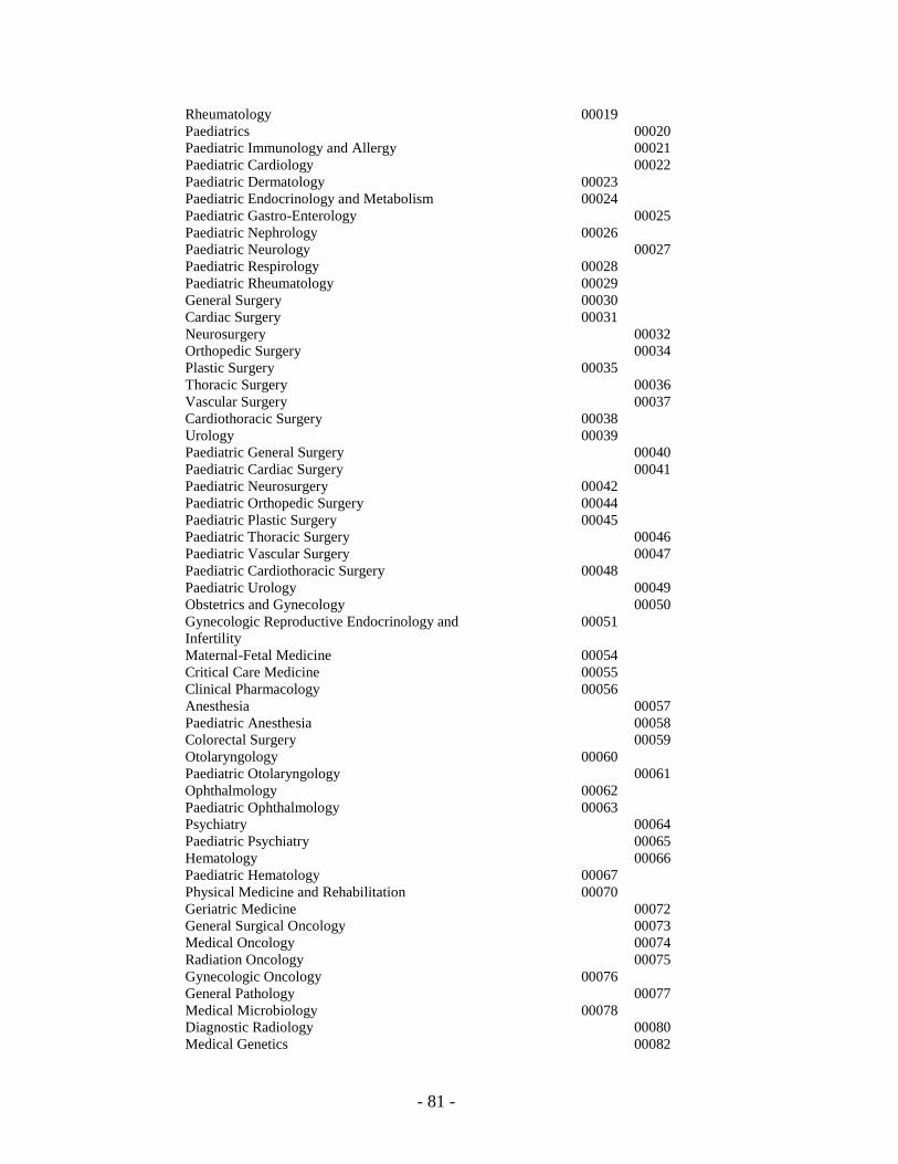
- 81 -

Rheumatology 00019

Paediatrics 00020

Paediatric Immunology and Allergy 00021

Paediatric Cardiology 00022

Paediatric Dermatology 00023

Paediatric Endocrinology and Metabolism 00024

Paediatric Gastro-Enterology 00025

Paediatric Nephrology 00026

Paediatric Neurology 00027

Paediatric Respirology 00028

Paediatric Rheumatology 00029

General Surgery 00030

Cardiac Surgery 00031

Neurosurgery 00032

Orthopedic Surgery 00034

Plastic Surgery 00035

Thoracic Surgery 00036

Vascular Surgery 00037

Cardiothoracic Surgery 00038

Urology 00039

Paediatric General Surgery 00040

Paediatric Cardiac Surgery 00041

Paediatric Neurosurgery 00042

Paediatric Orthopedic Surgery 00044

Paediatric Plastic Surgery 00045

Paediatric Thoracic Surgery 00046

Paediatric Vascular Surgery 00047

Paediatric Cardiothoracic Surgery 00048

Paediatric Urology 00049

Obstetrics and Gynecology 00050

Gynecologic Reproductive Endocrinology and 00051

Infertility

Maternal-Fetal Medicine 00054

Critical Care Medicine 00055

Clinical Pharmacology 00056

Anesthesia 00057

Paediatric Anesthesia 00058

Colorectal Surgery 00059

Otolaryngology 00060

Paediatric Otolaryngology 00061

Ophthalmology 00062

Paediatric Ophthalmology 00063

Psychiatry 00064

Paediatric Psychiatry 00065

Hematology 00066

Paediatric Hematology 00067

Physical Medicine and Rehabilitation 00070

Geriatric Medicine 00072

General Surgical Oncology 00073

Medical Oncology 00074

Radiation Oncology 00075

Gynecologic Oncology 00076

General Pathology 00077

Medical Microbiology 00078

Diagnostic Radiology 00080

Medical Genetics 00082

- 82 -

Anatomical Pathology 00083

Hematological Pathology 00085

Neuropathology 00086

Nuclear Medicine 00089

Medical Biochemistry 00090

Pediatric Radiology 00092

Neuroradiology 00093

Infectious Diseases 00096

Neonatal-Perinatal Medicine 00097

Non-Physician Services CIHI Provider

Service Number

Dentistry Group 01000

Dentist 01001

Dental Surgeon 01002

Oral Surgeon 01003

Orthodontist 01004

Paedodontist 01005

Periodontist 01006

Oral Pathologist 01007

Endodontist 01008

Oral Radiologist 01009

Dental Hygienist/Assistant 01010

Dental Mechanic 01011

Paediatric Oral Surgeon 01012

Paediatric Dentist 01013

Podiatry/Chiropody in General 02000

Podiatrist 02001

Chiropodist 02002

Therapist Group 03000

Radiotherapist 03001

Physiotherapist 03002

Occupational Therapist 03003

Respiratory Therapist 03004

Massage Therapist 03005

Psychotherapist 03006

Recreation Therapist 03007

Therapy Assistant 03008

Speech Language Pathologist 03009

Kinesiologist 03011

Rehabilitation Counsellor 03012

Physiotherapist Assistant 03013

Occupational Therapist Assistant 03014

Rehabilitation Therapist 03015

Rehabilitation Engineer 03016

Orthotist 03017

Prosthetist 03018

Vocational Rehabilitation Counsellor 03019

Audiologist 04000

Chiropractor 05000

Dietitian 06000

Osteopath 07000

Optometrist 08000

Ophthalmologic technician 08001

Orthoptician/Prosthetician 09000

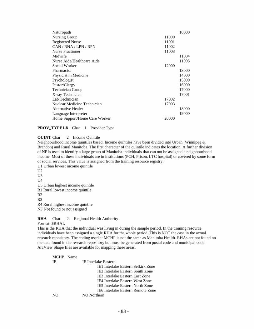
- 83 -

Naturopath 10000

Nursing Group 11000

Registered Nurse 11001

CAN / RNA / LPN / RPN 11002

Nurse Practioner 11003

Midwife 11004

Nurse Aide/Healthcare Aide 11005

Social Worker 12000

Pharmacist 13000

Physicist in Medicine 14000

Psychologist 15000

Pastor/Clergy 16000

Technician Group 17000

X-ray Technician 17001

Lab Technician 17002

Nuclear Medicine Technician 17003

Alternative Healer 18000

Language Interpreter 19000

Home Support/Home Care Worker 20000

PROV_TYPE1-8 Char 1 Provider Type

QUINT Char 2 Income Quintile

Neighbourhood income quintiles based. Income quintiles have been divided into Urban (Winnipeg &

Brandon) and Rural Manitoba. The first character of the quintile indicates the location. A further division

of NF is used to identify a large group of Manitoba individuals that can not be assigned a neighbourhood

income. Most of these individuals are in institutions (PCH, Prison, LTC hospital) or covered by some form

of social services. This value is assigned from the training resource registry.

U1 Urban lowest income quintile

U2

U3

U4

U5 Urban highest income quintile

R1 Rural lowest income quintile

R2

R3

R4 Rural highest income quintile

NF Not found or not assigned

RHA Char 2 Regional Health Authority

Format: $RHAL

This is the RHA that the individual was living in during the sample period. In the training resource

individuals have been assigned a single RHA for the whole period. This is NOT the case in the actual

research repository. The coding used at MCHP is not the same as Manitoba Health. RHAs are not found on

the data found in the research repository but must be generated from postal code and municipal code.

ArcView Shape files are available for mapping these areas.

MCHP Name

IE IE Interlake Eastern

IE1 Interlake Eastern Selkirk Zone

IE2 Interlake Eastern South Zone

IE3 Interlake Eastern East Zone

IE4 Interlake Eastern West Zone

IE5 Interlake Eastern North Zone

IE6 Interlake Eastern Remote Zone

NO NO Northern

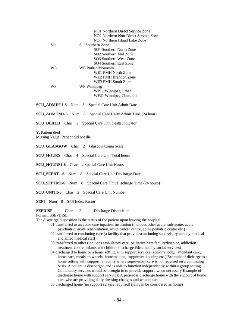
- 84 -

NO1 Northern Direct Service Zone

NO2 Northern Non-Direct Service Zone

NO3 Northern Island Lake Zone

SO SO Southern Zone

SO1 Southern North Zone

SO2 Southern Mid Zone

SO3 Southern West Zone

SO4 Southern East Zone

WE WE Prairie Mountain

WE1 PMH North Zone

WE2 PMH Brandon Zone

WE3 PMH South Zone

WP WP Winnipeg

WP11 Winnipeg Urban

WP21 Winnipeg Churchill

SCU_ADMDT1-6 Num 8 Special Care Unit Admit Date

SCU_ADMTM1-6 Num 8 Special Care Unity Admit Time (24 hour)

SCU_DEATH Char 1 Special Care Unit Death Indicator

Y. Patient died

Missing Value. Patient did not die

SCU_GLASGOW Char 2 Glasgow Coma Scale

SCU_HOURS Char 4 Special Care Unit Total hours

SCU_HOURS1-6 Char 4 Special Care Unit Hours

SCU_SEPDT1-6 Num 8 Special Care Unit Discharge Date

SCU_SEPTM1-6 Num 8 Special Care Unit Discharge Time (24 hours)

SCU_UNIT1-6 Char 2 Special Care Unit Number

SEFI Num 8 SES Index Factor

SEPDISP Char 2 Discharge Disposition

Format: $SEPDISL

The discharge disposition is the status of the patient upon leaving the hospital

01 transferred to an acute care inpatient institution (includes other acute, sub-acute, acute

psychiatric, acute rehabilitation, acute cancer centre, acute pediatric centre etc.)

02 transferred to continuing care (a facility that providescontinuing supervisory care by medical

and allied medical staff)

03 transferred to other (includes ambulatory care, palliative care facility/hospice, addiction

treatment centre, infants and children discharged/detained by social services)

04 discharged to home or a home setting with support services (senior’s lodge, attendant care,

home care, meals on wheels, homemaking, supportive housing etc.) Example of dicharge to a

home setting with support: a facility where supervisory care is not required on a continuing

basis. A patient is discharged and is able to function independently within a group setting.

Community services would be brought in to provide support, when necessary Example of

discharge home with support services: A patient is discharge home with the support of home

care who are providing daily dressing changes and wound care

05 discharged home (no support service required) (jail can be considered as home)

- 85 -

06 left against medical advice (with or without signout, AWOL)

07 died

08 cadaveric donor admitted for organ/tissue retrieval

09 stillbirth

10 newborn and pediatric discharged to Child and Family Services (Manitoba only)

11 private adoption of newborn (Manitoba only)

12 Patients who did not return from a pass

SEPDT NUM Separation Date

Range: 20040401-20140415

Date of separation from hospital. SAS date format yymmdd10.

SERV1-3 Char 2 Patient Service Transfer

SERVDAYS1-3 Char 5 Patient Service Transfer Days

SEX Char 1 Biological gender

Format: $SEXF

SUBSERV Char 1 Main Patient Sub-service

For further specification of the main patient service a one digit subservice code can be added. This optional

code allows the client to further differentiate types of patients treated within a patient service.

SUBSERV1-3 Char 1 Patient Sub-service transfer

This one digit code may be defined by the client to further specify the patient service transfer.

TEACHING Char 1 Teaching Hospital code

Teaching hospital records in the training database are identified with a ‘1’.

TRANSACT Char 1 Transaction Code

Identify Inpatient (‘1’) and Day Surgery records (‘3’). Note LOS is measured in different units for Inpatient

and Day Surgery records.

TRFROMF Char 1 Transfer from code

This variable flags if there is a transfer from code (value=’1’) found on the original record. The hospital

abstracts in the research repository indicate the hospital code where the transfer was from. These variables

are modified from the original variables found in the research repository.

TRTOF Char 1 Transfer to code

This variable flags if there is a transfer to code (value=’1’) found on the original record. The hospital

abstracts in the research repository indicate the hospital code where the transfer was to. These variables are

modified from the original variables found in the research repository.

WEIGHT Num 8 Newborn/Neonate Weight

WPG_CA Char 3 Winnipeg Community Areas

Format: $RHAL

These are Winnipeg subregions similar in size the non-Winnipeg RHAs. Note there are a small number of

individuals with a Winnipeg RHA (K) that are not assigned to a Winnipeg Community area. Winnipeg

areas are not found on the data found in the research repository but must be generated from postal code and

municipal code. ArcView Shape files are available for mapping these areas.

W02 ASSINIBOINE SOUTH

W11 DOWNTOWN

W03 FORT GARRY

W09 INKSTER

- 86 -

W10 POINT DOUGLAS

W07 RIVER EAST

W12 RIVER HEIGHTS

W08 SEVEN OAKS

W04 ST. VITAL

W05 ST.BONIFACE

W01 ST.JAMES-ASSINIBOIA

W06 TRANSCONA

Physician Medical Services Dictionary

This dataset is part of the MCHP SAS Course database. Use of this data must be accompanied by the

‘MCHP SAS Workshop Simulated Administrative Health Data Use Agreement’. The datasets in this

resource have been simulated using distributions of services within the Manitoba population which means

that analysis for course should be representative of services and outcomes within Manitoba from 2005/06-

2013/14.

NOTE: This data is not real and any correspondence to actual events, people or services are only

coincidental.

The Physician Claims data contains visits to physicians by individuals found in the course REGISTRY file.

In some cases claims are for services provided during an inpatient hospital stay.

These data represent 1578147 observations and 21 variables.

Name of resource: MEDICAL

AMBVIS Num 3 Ambulatory Visit Flag

This flag identifies ambulatory visits as used at MCHP (‘1’ – Ambulatory visit)

BIRTHDT Char 8 Birth Date (mod)

Date of birth from the training resource registry file. SAS date variable (YYMMDD10.)

age =floor(yrdif(birthdt,servdt,'age'));

SERVDT NUM 8 Date of service

Range: 19000116 - 21000104

This is the year-month-day format of patient’s visit or other service provided by billing physician.

DIAG Char 3 Diagnosis

This is the ICD-9-CM diagnosis codes provided on billing. Some DIAG fields are blank.

FEE Num 5 Fee for service

Range: -8-$8310.80

This is the fee that was billed for this service.

HOSPRHA Char 2 RHA of Hospital

This is the RHA location of the Hospital. See RHA for codes. Note in the research registry the hospital

number will contain a provincial code for out of province services.

ID Char 6 Personal ID Number (Mod)

This is a personal identifier that can be used in all of the training resource data. It is NOT related to PHIN

or family registration number. This number is assigned from the training resource registry.

- 87 -

IN_HOSP Num 3 In Hosp Confirmed Flag

MDBLOC Char 3 md bloc + subbloc

Format: $BLOCSBL

This is the field of practice that MDNO has registered with the Manitoba College of Physicians and

Surgeons.

'01' = 'Internal Medicine'

'011'= 'Int.Med - Neurology'

'012'= 'Int.Med - Geriatrics'

'013'= 'Int.Med - Rheumatology'

‘014’= ‘Int. Med – Cardiology

‘015’= ‘Int. Med – Gastroenterology’

‘016’= ‘Int. Med – Nephrology’

‘017’= ‘Intmed – Allergy/Clinical Immunology’

'018'= 'Int.Med - Genetics'

'019'= 'Int.Med - OOP'

'02' = 'Pediatrics'

'029'= 'Pediatrics - OOP'

'03' = 'Psychiatry'

'039'= 'Psychiatry - OOP'

'04' = 'Surgery - unspecified'

'040'= 'Surgery - Oral'

'041'= 'Surgery - General'

'042'= 'Surgery - Thoracic & CV'

'043'= 'Surgery - Plastic'

'044'= 'Surgery - Urology'

'045'= 'Surgery - Orthopedic'

'046'= 'Surgery - Neurology'

'047'= 'Surgery - Dental'

'048'= 'Surgery - Peridontal'

'049'= 'Surgery - OOP'

'051'= 'ENT - Eye only'

'052'= 'ENT - Other than eye'

'053'= 'ENT - Optometry'

'059'= 'ENT - OOP'

'06' = 'Dermatology'

'069'= 'Dermatology - OOP'

'07' = 'Radiology'

'071'= 'Radiology - In-hospital'

'072'= 'Radiology - Professional'

‘073’= ‘Radiology – Nuclear Medicine Split’

‘074;= ‘Radiology – Nuclear Medicine Prof’

‘075’= ‘Radiology – Nuclear medicine Total

'076'= 'Radiology - Ultra Sound & MIR'

'079'= 'Radiology - OOP'

'08' = 'Pathology'

'081' ='Pathology - Anatomical'

'082' ='Pathology - Heamatological'

'083' ='Pathology - Medical Biochemistry'

'084' ='Pathology - Medical Microbiology'

'085' ='Pathology - Neuropathology'

'089'= 'Pathology - OOP'

'09' = 'Obstetrics & Gynecology'

'091'= 'Perinatal Medicine'

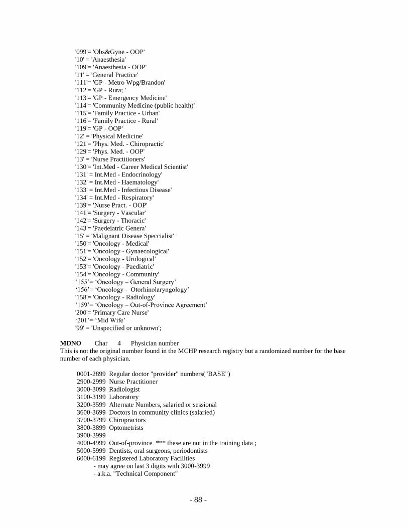
- 88 -

'099'= 'Obs&Gyne - OOP'

'10' = 'Anaesthesia'

'109'= 'Anaesthesia - OOP'

'11' = 'General Practice'

'111'= 'GP - Metro Wpg/Brandon'

'112'= 'GP - Rura; '

'113'= 'GP - Emergency Medicine'

'114'= 'Community Medicine (public health)'

'115'= 'Family Practice - Urban'

'116'= 'Family Practice - Rural'

'119'= 'GP - OOP'

'12' = 'Physical Medicine'

'121'= 'Phys. Med. - Chiropractic'

'129'= 'Phys. Med. - OOP'

'13' = 'Nurse Practitioners'

'130'= 'Int.Med - Career Medical Scientist'

'131' = Int.Med - Endocrinology'

'132' = Int.Med - Haematology'

'133' = Int.Med - Infectious Disease'

'134' = Int.Med - Respiratory'

'139'= 'Nurse Pract. - OOP'

'141'= 'Surgery - Vascular'

'142'= 'Surgery - Thoracic'

'143'= 'Paedeiatric Genera'

'15' = 'Malignant Disease Speccialist'

'150'= 'Oncology - Medical'

'151'= 'Oncology - Gynaecological'

'152'= 'Oncology - Urological'

'153'= 'Oncology - Paediatric'

'154'= 'Oncology - Community'

‘155’= ‘Oncology – General Surgery’

‘156’= ‘Oncology - Otorhinolaryngology’

'158'= 'Oncology - Radiology'

‘159’= ‘Oncology – Out-of-Province Agreement’

'200'= 'Primary Care Nurse'

‘201’= ‘Mid Wife’

'99' = 'Unspecified or unknown';

MDNO Char 4 Physician number

This is not the original number found in the MCHP research registry but a randomized number for the base

number of each physician.

0001-2899 Regular doctor "provider" numbers("BASE")

2900-2999 Nurse Practitioner

3000-3099 Radiologist

3100-3199 Laboratory

3200-3599 Alternate Numbers, salaried or sessional

3600-3699 Doctors in community clinics (salaried)

3700-3799 Chiropractors

3800-3899 Optometrists

3900-3999

4000-4999 Out-of-province *** these are not in the training data ;

5000-5999 Dentists, oral surgeons, periodontists

6000-6199 Registered Laboratory Facilities

- may agree on last 3 digits with 3000-3999

- a.k.a. "Technical Component"

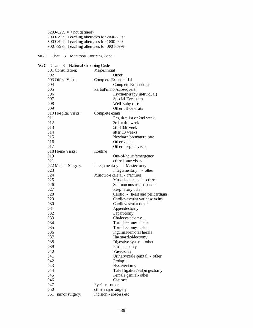
- 89 -

6200-6299 = < not defined>

7000-7999 Teaching alternates for 2000-2999

8000-8999 Teaching alternates for 1000-999

9001-9998 Teaching alternates for 0001-0998

MGC Char 3 Manitoba Grouping Code

NGC Char 3 National Grouping Code

001 Consultation: Major/initial

002 Other

003 Office Visit: Complete Exam-initial

004 Complete Exam-other

005 Partial/minor/subsequent

006 Psychotherapy(individual)

007 Special Eye exam

008 Well Baby care

009 Other office visits

010 Hospital Visits: Complete exam

011 Regular: 1st or 2nd week

012 3rd or 4th week

013 5th-13th week

014 after 13 weeks

015 Newborn/premature care

016 Other visits

017 Other hospital visits

018 Home Visits: Routine

019 Out-of-hours/emergency

021 other home visits

022 Major Surgery: Integumentary - Mastectomy

023 Integumentary - other

024 Musculo-skeletal - fractures

025 Musculo-skeletal - other

026 Sub-mucous resection,etc

027 Respiratory other

028 Cardio - heart and pericardium

029 Cardiovascular varicose veins

030 Cardiovascular other

031 Appendectomy

032 Laparotomy

033 Cholecystectomy

034 Tonsillectomy - child

035 Tonsillectomy - adult

036 Inguinal/femoral hernia

037 Haemorrhoidectomy

038 Digestive system - other

039 Prostatectomy

040 Vasectomy

041 Urinary/male genital - other

042 Prolapse

043 Hysterectomy

044 Tubal ligation/Salpingectomy

045 Female genital- other

046 Cataract

047 Eye/ear - other

050 other major surgery

051 minor surgery: Incision - abscess,etc

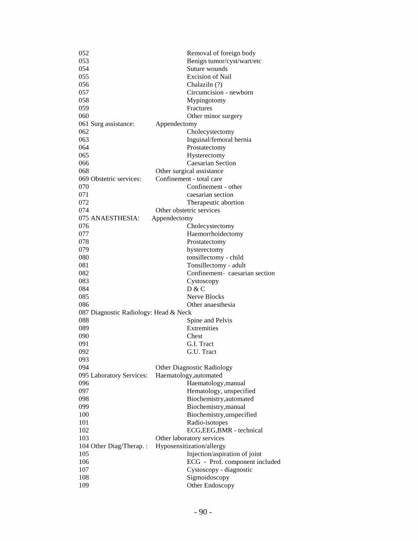
- 90 -

052 Removal of foreign body

053 Benign tumor/cyst/wart/etc

054 Suture wounds

055 Excision of Nail

056 Chalaziln (?)

057 Circumcision - newborn

058 Mypingotomy

059 Fractures

060 Other minor surgery

061 Surg assistance: Appendectomy

062 Cholecystectomy

063 Inguinal/femoral hernia

064 Prostatectomy

065 Hysterectomy

066 Caesarian Section

068 Other surgical assistance

069 Obstetric services: Confinement - total care

070 Confinement - other

071 caesarian section

072 Therapeutic abortion

074 Other obstetric services

075 ANAESTHESIA: Appendectomy

076 Cholecystectomy

077 Haemorrhoidectomy

078 Prostatectomy

079 hysterectomy

080 tonsillectomy - child

081 Tonsillectomy - adult

082 Confinement- caesarian section

083 Cystoscopy

084 D & C

085 Nerve Blocks

086 Other anaesthesia

087 Diagnostic Radiology: Head & Neck

088 Spine and Pelvis

089 Extremities

090 Chest

091 G.I. Tract

092 G.U. Tract

093

094 Other Diagnostic Radiology

095 Laboratory Services: Haematology,automated

096 Haematology,manual

097 Hematology, unspecified

098 Biochemistry,automated

099 Biochemistry,manual

100 Biochemistry,unspecified

101 Radio-isotopes

102 ECG,EEG,BMR - technical

103 Other laboratory services

104 Other Diag/Therap. : Hyposensitization/allergy

105 Injection/aspiration of joint

106 ECG - Prof. component included

107 Cystoscopy - diagnostic

108 Sigmoidoscopy

109 Other Endoscopy

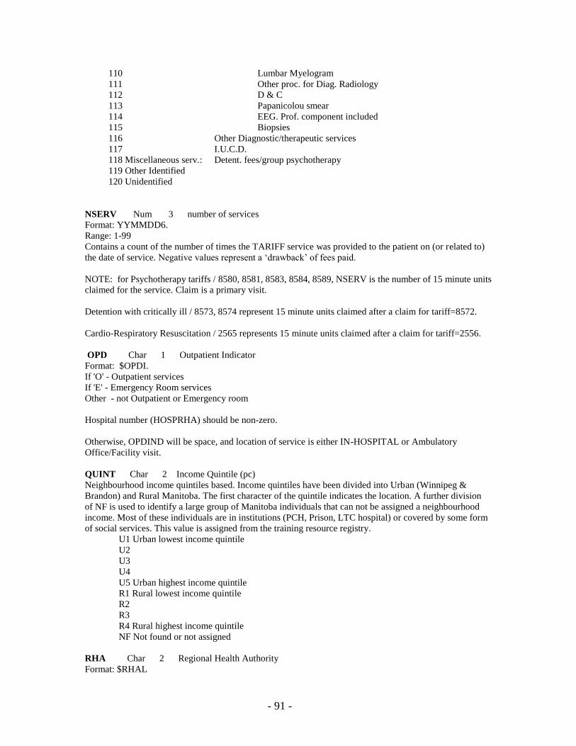
- 91 -

110 Lumbar Myelogram

111 Other proc. for Diag. Radiology

112 D & C

113 Papanicolou smear

114 EEG. Prof. component included

115 Biopsies

116 Other Diagnostic/therapeutic services

117 I.U.C.D.

118 Miscellaneous serv.: Detent. fees/group psychotherapy

119 Other Identified

120 Unidentified

NSERV Num 3 number of services

Format: YYMMDD6.

Range: 1-99

Contains a count of the number of times the TARIFF service was provided to the patient on (or related to)

the date of service. Negative values represent a ‘drawback’ of fees paid.

NOTE: for Psychotherapy tariffs / 8580, 8581, 8583, 8584, 8589, NSERV is the number of 15 minute units

claimed for the service. Claim is a primary visit.

Detention with critically ill / 8573, 8574 represent 15 minute units claimed after a claim for tariff=8572.

Cardio-Respiratory Resuscitation / 2565 represents 15 minute units claimed after a claim for tariff=2556.

OPD Char 1 Outpatient Indicator

Format: $OPDI.

If 'O' - Outpatient services

If 'E' - Emergency Room services

Other - not Outpatient or Emergency room

Hospital number (HOSPRHA) should be non-zero.

Otherwise, OPDIND will be space, and location of service is either IN-HOSPITAL or Ambulatory

Office/Facility visit.

QUINT Char 2 Income Quintile (pc)

Neighbourhood income quintiles based. Income quintiles have been divided into Urban (Winnipeg &

Brandon) and Rural Manitoba. The first character of the quintile indicates the location. A further division

of NF is used to identify a large group of Manitoba individuals that can not be assigned a neighbourhood

income. Most of these individuals are in institutions (PCH, Prison, LTC hospital) or covered by some form

of social services. This value is assigned from the training resource registry.

U1 Urban lowest income quintile

U2

U3

U4

U5 Urban highest income quintile

R1 Rural lowest income quintile

R2

R3

R4 Rural highest income quintile

NF Not found or not assigned

RHA Char 2 Regional Health Authority

Format: $RHAL

- 92 -

This is the RHA that the individual was living in during the sample period. In the training resource

individuals have been assigned a single RHA for the whole period. This is NOT the case in the actual

research repository. The coding used at MCHP is not the same as Manitoba Health. ArcView Shape files

are available for mapping these areas.

MCHP Name

IE IE Interlake Eastern

IE1 Interlake Eastern Selkirk Zone

IE2 Interlake Eastern South Zone

IE3 Interlake Eastern East Zone

IE4 Interlake Eastern West Zone

IE5 Interlake Eastern North Zone

IE6 Interlake Eastern Remote Zone

NO NO Northern

NO1 Northern Direct Service Zone

NO2 Northern Non-Direct Service Zone

NO3 Northern island Lake Zone

SO SO Southern Zone

SO1 Southern North Zone

SO2 Southern Mid Zone

SO3 Southern West Zone

SO4 Southern East Zone

WE WE Prairie Mountain

WE1 PMH North Zone

WE2 PMH Brandon Zone

WE3 PMH South Zone

WP WP Winnipeg

WP11 Winnipeg Urban

WP21 Winnipeg Churchill

SEFI Num 8 SES Factor Index

SEX Char 1 Biological gender of individual

Format: $SEXF.

1 Male

2 Female

TARIFF Char 4 Tariff code – Services rendered

Defines specific services for which a physician may bill Manitoba Health. Often requires prefix code,

TARPREF, to determine the appropriate situation and type of service being claimed.

This is subject to annual review and redefinition of "covered” services. A specific code may have different

meanings depending on the fiscal year of the claim. Some codes may split into two or more new codes,

others may be combined into a single code.

May be "0000" - Local anaesthesia if TARPREF = 4 or 6.

May be "9999" - By report, new or special Services

TEACHING Char 1 Teaching Hospital

This indicates if the hospital is a teaching hospital.

WPG_CA Char 3 Winnipeg Community Areas

Format: $RHAL

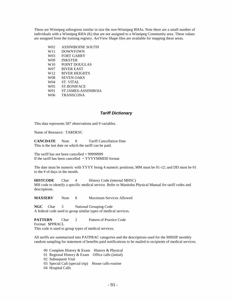
- 93 -

These are Winnipeg subregions similar in size the non-Winnipeg RHAs. Note there are a small number of

individuals with a Winnipeg RHA (K) that are not assigned to a Winnipeg Community area. These values

are assigned from the training registry. ArcView Shape files are available for mapping these areas.

W02 ASSINIBOINE SOUTH

W11 DOWNTOWN

W03 FORT GARRY

W09 INKSTER

W10 POINT DOUGLAS

W07 RIVER EAST

W12 RIVER HEIGHTS

W08 SEVEN OAKS

W04 ST. VITAL

W05 ST.BONIFACE

W01 ST.JAMES-ASSINIBOIA

W06 TRANSCONA

Tariff Dictionary

This data represents 587 observations and 9 variables.

Name of Resource: TARDESC

CANCDATE Num 8 Tariff Cancellation Date

This is the last date on which the tariff can be paid.

The tariff has not been cancelled = 99999999

If the tariff has been cancelled = YYYYMMDD format

The date must be numeric with YYYY being 4 numeric positions; MM must be 01-12; and DD must be 01

to the # of days in the month.

HISTCODE Char 4 History Code (internal MHSC)

MH code to identify a specific medical service. Refer to Manitoba Physical Manual for tariff codes and

descriptions.

MAXSERV Num 8 Maximum Services Allowed

NGC Char 3 National Grouping Code

A federal code used to group similar types of medical services.

PATTERN Char 2 Pattern of Practice Code

Format: $PPRACL

This code is used to group types of medical services.

All tariffs are summarized into PATPRAC categories and the descriptions used for the MHSIP monthly

random sampling for statement of benefits paid notifications to be mailed to recipients of medical services.

00 Complete History & Exam History & Physical

01 Regional History & Exam Office calls (initial)

02 Subsequent Visit

03 Special Call (special trip) House calls-routine

04 Hospital Calls

- 94 -

05 Consultation

06 Anaesthesia - surgical

07 Anaesthesia - obstetrical

08 x-ray - Head, Neck

09 x-ray - Chest

10 x-ray - Spine, Pelvis

11 x-ray - Upper Extremities

12 x-ray - Lower Extremities

13 x-ray - Abdomen

14 x-ray - Urological

15 x-ray - Obstetrical. & Gynaecological.

16 x-ray - Special

17 x-ray - Therapeutic

18 x-ray - Radium

19 Laboratory

20 Laboratory - short list tariffs

21 Heart Tracing "ECG"

22 Eye Test Refractions

23 Allergy Care

24 Immunization

25 Injection

26 Surgery Surgery >= $50.00

27 Diagnostic/therapeutic serv. Surgery <$50.00

28 Surgical assistance

29 Other Tests and exams

30 Laboratory Smear Cytological smears

31 Obstetrics Confinements

32 Caesarian

33 Obstetrics Abortions

34 Obstetrics Ectopic

35 Oral Surgery Dental surgery

36 Emergency Visit House visit- emergency

37 Hospital Misc. Elec. shock-therapy

38 Concomitant Care

39 Chiropractor - subsequent visit

40 Chiropractor - initial visit

41 Optometrist - eye test

42 Routine Visit/Chronic Care (PCH)

PREFIX Char 1 Tariff Prefix

Format: $TARPFL

This defines the circumstances or sub-component of a tariff classification which was applied to this claim

when determining FEEPAID or grouping services into general categories for monthly reports produced by

MHSIP.

Value MUST be one of:

0 Surgical assistance

1 Post-operative Fee

2 Surgery

3 Maternity

4 Anaesthetic

5 X-ray/radiology

6 Anaesthesia assistance

7 Calls, Special tests

8 Pathology/laboratory

- 95 -

9 undefined i.e. New procedure or procedure not

covered by fee schedule.

SEXREST Char 1 Sex Restriction Code (M/F)

This code is used whenever there is a restriction for a specific tariff record.

M Patient’s sex must be male

F Patient’s sex must be female

TARDES Char 90 Tariff Description

A description of the service provided for under the tariff code.

TARIFF Char 4 Tariff Code – Services Rendered

Defines specific services for which a physician may bill Manitoba Health. Often requires prefix code,

TARPREF, to determine the appropriate situation and type of service being claimed.

This is subject to annual review and redefinition of "covered” services. A specific code may have different

meanings depending on the fiscal year of the claim. Some codes may split into two or more new codes,

others may be combined into a single code.

May be "0000" - Local anaesthesia if TARPREF = 4 or 6.

May be "9999" - By report, new or special Services

Registry Dictionary

This dataset is part of the MCHP SAS Course database. Use of this data must be accompanied by the

‘MCHP SAS Workshop Simulated Administrative Health Data Use Agreement’. The datasets in this

resource have been simulated using distributions of services within the Manitoba population which means

that analysis for course should be representative of services and outcomes within Manitoba over the period

2005/06 – 2013/14. The data represents an approximate 1% of the actual population.

NOTE: This data is not real and any correspondence to actual events, people or services are only

coincidental.

This dataset may contain multiple records for each individual if there are breaks or changes in coverage.

These data represent 15108 observations and 10 variables.

Name of resource: REGISTRY

BIRTHDT Char 8 Birth Date (mod)

This is the birth date for the individual as a character string in the format yymmdd8. There are a number of

birth dates that have 00 for the day and/or month. These should be corrected when using birth. This

variable is modified from the original date of birth found in the research repository.

age =floor(birth,covenddate,'act/act'));

COVCANCODE Char 1 Coverage Cancel Code or Cancel Reason

This is the reason for cancellation of coverage in the registry. There are only three codes in this database.

This variable is modified from the original cancellation code in the research repository.

0 = Not canceled (still active and in province)

2 = Died (COVENDDATE) will be the date of death

Other= Other – loss to follow-up

- 96 -

COVENDDATE NUM 8 End of Coverage Date (mod)

Range: 19990403 - 20121122

This is the last date of coverage. Dates beyond 20100401 (April 1, 2010) indicate ongoing coverage for the

purposes of this file.

COVSTARTDATE Char 8 Start of Coverage Date (mod)

Range: 19570629 - 20090330

This is the first date of coverage. In this registry individuals are considered living in Manitoba between the

coverage start and coverage end dates. In the actual registry there may be gaps in coverage for individuals.

ID Char 6 Personal ID Number (Mod)

This is a personal identifier that can be used in all of the training resource data. It is NOT related to PHIN

or family registration number.

QUINT Char 2 Income Quintile (pc)

Neighbourhood income quintiles based. Income quintiles have been divided into Urban (Winnipeg &

Brandon) and Rural Manitoba. The first character of the quintile indicates the location. A further division

of NF is used to identify a large group of Manitoba individuals that can not be assigned a neighbourhood

income. Most of these individuals are in institutions (PCH, Prison, LTC hospital) or covered by some form

of social services. Income groups are not found on the data found in the research repository but must be

generated from postal code and municipal code.

U1 Urban lowest income quintile

U2

U3

U4

U5 Urban highest income quintile

R1 Rural lowest income quintile

R2

R3

R4

R5 Rural highest income quintile

NF Not found or not assigned

RHA Char 2 Regional Health Authority

Format: $RHAL

This is the RHA that the individual was living in during the sample period. In the training resource

individuals have been assigned a single RHA for the whole period. This is NOT the case in the actual

research repository. The coding used at MCHP is not the same as Manitoba Health. RHAs are not found on

the data found in the research repository but must be generated from postal code and municipal code.

ArcView Shape files are available for mapping these areas.

MCHP Name

IE IE Interlake Eastern

IE1 Interlake Eastern Selkirk Zone

IE2 Interlake Eastern South Zone

IE3 Interlake Eastern East Zone

IE4 Interlake Eastern West Zone

IE5 Interlake Eastern North Zone

IE6 Interlake Eastern Remote Zone

NO NO Northern

NO1 Northern Direct Service Zone

NO2 Northern Non-Direct Service Zone

NO3 Northern island Lake Zone

SO SO Southern Zone

SO1 Southern North Zone

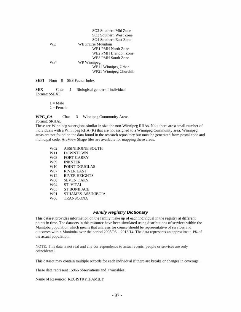
- 97 -

SO2 Southern Mid Zone

SO3 Southern West Zone

SO4 Southern East Zone

WE WE Prairie Mountain

WE1 PMH North Zone

WE2 PMH Brandon Zone

WE3 PMH South Zone

WP WP Winnipeg

WP11 Winnipeg Urban

WP21 Winnipeg Churchill

SEFI Num 8 SES Factor Index

SEX Char 1 Biological gender of individual

Format: $SEXF

1 = Male

2 = Female

WPG_CA Char 3 Winnipeg Community Areas

Format: $RHAL

These are Winnipeg subregions similar in size the non-Winnipeg RHAs. Note there are a small number of

individuals with a Winnipeg RHA (K) that are not assigned to a Winnipeg Community area. Winnipeg

areas are not found on the data found in the research repository but must be generated from postal code and

municipal code. ArcView Shape files are available for mapping these areas.

W02 ASSINIBOINE SOUTH

W11 DOWNTOWN

W03 FORT GARRY

W09 INKSTER

W10 POINT DOUGLAS

W07 RIVER EAST

W12 RIVER HEIGHTS

W08 SEVEN OAKS

W04 ST. VITAL

W05 ST.BONIFACE

W01 ST.JAMES-ASSINIBOIA

W06 TRANSCONA

Family Registry Dictionary

This dataset provides information on the family make up of each individual in the registry at different

points in time. The datasets in this resource have been simulated using distributions of services within the

Manitoba population which means that analysis for course should be representative of services and

outcomes within Manitoba over the period 2005/06 – 2013/14. The data represents an approximate 1% of

the actual population.

NOTE: This data is not real and any correspondence to actual events, people or services are only

coincidental.

This dataset may contain multiple records for each individual if there are breaks or changes in coverage.

These data represent 15966 observations and 7 variables.

Name of Resource: REGISTRY_FAMILY

- 98 -

BIRTHORD Num 8 Birth Order in Family

ENDDATE Char 8

Range: 19660101- 20121122

This is the end date of the combination of reltype, nsib, and birthord. Each id can have multiple records

based on their changing family structure.

ID Char 6 Personal ID Number (Mod)

This is a personal identifier that can be used in all of the training resource data. It is NOT related to PHIN

or family registration number. This number is assigned from the training resource registry.

MARST Char 1 Marital Status

This describes whether the individual is married or not. This can be used in conjunction with RELTYPE to

determine if the individual is head of the household.

0 Not Married

1 Married

Blank Dependent child

NSIB Num 8 Number of Siblings

RELTYPE Char 1 Type of Individual (family head/spouse/child)

Format: $RTYPE

1 Head of household

2 Spouse

5 Dependent child

STARTDATE Char 8

Range: 19570629- 20101130

This is the start date of the combination of reltype, nsib, and birthord. Each id can have multiple records

based on their changing family structure.

Census Dictionary

This dataset is part of the MCHP SAS Course database. Use of this data must be accompanied by the

‘MCHP SAS Workshop Simulated Administrative Health Data Use Agreement’. The datasets in this

resource have been simulated using distributions of services within the Manitoba population which means

that analysis for course should be representative of services and outcomes within Manitoba.

The following document provides the variable names and some basic information on the census data

associated with each individual found in the training resource REGISTRY database. The data is aggregated

information for the area (usually DA) where the individual was living. The information includes variable

type, general description, and the data values for each variable. The data represents 15108 observations and

140 or 136 variables and covers two time periods (2006 and 2011).

Name of Resource: CENSUSXXXX (where XXXX is 2006 or 2011)

BIRTHDT Num 8 Birthdate (mod)

CC_F_AREA Num 8 Population & Dwelling – Total area

Only occurs in the 2006 data.

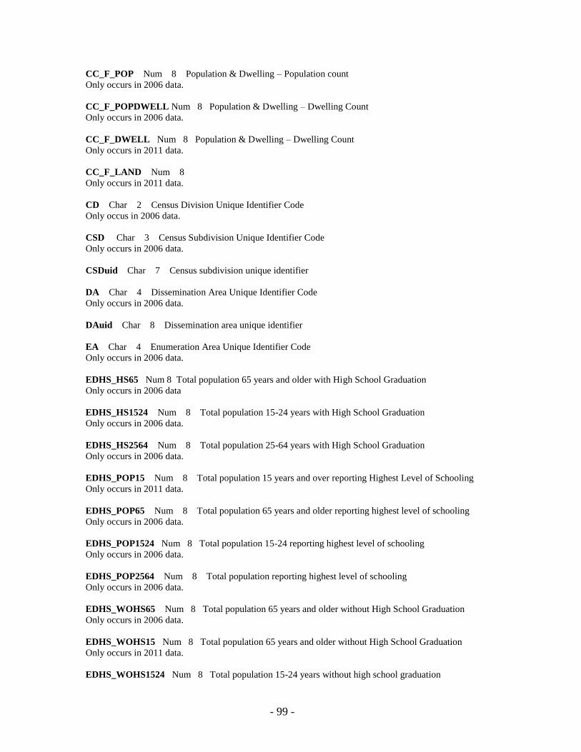
- 99 -

CC_F_POP Num 8 Population & Dwelling – Population count

Only occurs in 2006 data.

CC_F_POPDWELL Num 8 Population & Dwelling – Dwelling Count

Only occurs in 2006 data.

CC_F_DWELL Num 8 Population & Dwelling – Dwelling Count

Only occurs in 2011 data.

CC_F_LAND Num 8

Only occurs in 2011 data.

CD Char 2 Census Division Unique Identifier Code

Only occus in 2006 data.

CSD Char 3 Census Subdivision Unique Identifier Code

Only occurs in 2006 data.

CSDuid Char 7 Census subdivision unique identifier

DA Char 4 Dissemination Area Unique Identifier Code

Only occurs in 2006 data.

DAuid Char 8 Dissemination area unique identifier

EA Char 4 Enumeration Area Unique Identifier Code

Only occurs in 2006 data.

EDHS_HS65 Num 8 Total population 65 years and older with High School Graduation

Only occurs in 2006 data

EDHS_HS1524 Num 8 Total population 15-24 years with High School Graduation

Only occurs in 2006 data.

EDHS_HS2564 Num 8 Total population 25-64 years with High School Graduation

Only occurs in 2006 data.

EDHS_POP15 Num 8 Total population 15 years and over reporting Highest Level of Schooling

Only occurs in 2011 data.

EDHS_POP65 Num 8 Total population 65 years and older reporting highest level of schooling

Only occurs in 2006 data.

EDHS_POP1524 Num 8 Total population 15-24 reporting highest level of schooling

Only occurs in 2006 data.

EDHS_POP2564 Num 8 Total population reporting highest level of schooling

Only occurs in 2006 data.

EDHS_WOHS65 Num 8 Total population 65 years and older without High School Graduation

Only occurs in 2006 data.

EDHS_WOHS15 Num 8 Total population 65 years and older without High School Graduation

Only occurs in 2011 data.

EDHS_WOHS1524 Num 8 Total population 15-24 years without high school graduation

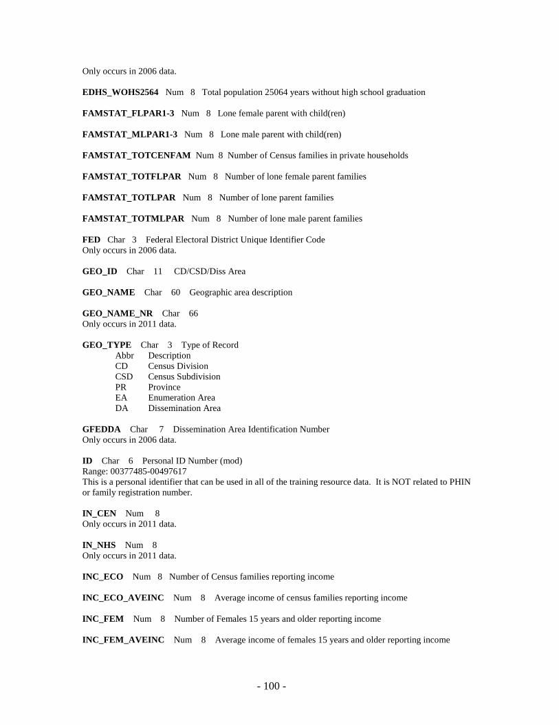
- 100 -

Only occurs in 2006 data.

EDHS_WOHS2564 Num 8 Total population 25064 years without high school graduation

FAMSTAT_FLPAR1-3 Num 8 Lone female parent with child(ren)

FAMSTAT_MLPAR1-3 Num 8 Lone male parent with child(ren)

FAMSTAT_TOTCENFAM Num 8 Number of Census families in private households

FAMSTAT_TOTFLPAR Num 8 Number of lone female parent families

FAMSTAT_TOTLPAR Num 8 Number of lone parent families

FAMSTAT_TOTMLPAR Num 8 Number of lone male parent families

FED Char 3 Federal Electoral District Unique Identifier Code

Only occurs in 2006 data.

GEO_ID Char 11 CD/CSD/Diss Area

GEO_NAME Char 60 Geographic area description

GEO_NAME_NR Char 66

Only occurs in 2011 data.

GEO_TYPE Char 3 Type of Record

Abbr Description

CD Census Division

CSD Census Subdivision

PR Province

EA Enumeration Area

DA Dissemination Area

GFEDDA Char 7 Dissemination Area Identification Number

Only occurs in 2006 data.

ID Char 6 Personal ID Number (mod)

Range: 00377485-00497617

This is a personal identifier that can be used in all of the training resource data. It is NOT related to PHIN

or family registration number.

IN_CEN Num 8

Only occurs in 2011 data.

IN_NHS Num 8

Only occurs in 2011 data.

INC_ECO Num 8 Number of Census families reporting income

INC_ECO_AVEINC Num 8 Average income of census families reporting income

INC_FEM Num 8 Number of Females 15 years and older reporting income

INC_FEM_AVEINC Num 8 Average income of females 15 years and older reporting income

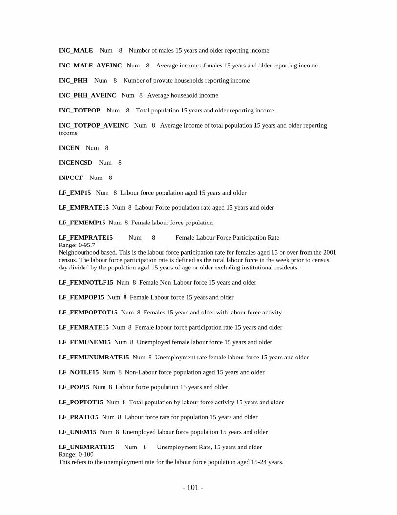
- 101 -

INC_MALE Num 8 Number of males 15 years and older reporting income

INC_MALE_AVEINC Num 8 Average income of males 15 years and older reporting income

INC_PHH Num 8 Number of provate households reporting income

INC_PHH_AVEINC Num 8 Average household income

INC_TOTPOP Num 8 Total population 15 years and older reporting income

INC_TOTPOP_AVEINC Num 8 Average income of total population 15 years and older reporting

income

INCEN Num 8

INCENCSD Num 8

INPCCF Num 8

LF_EMP15 Num 8 Labour force population aged 15 years and older

LF_EMPRATE15 Num 8 Labour Force population rate aged 15 years and older

LF_FEMEMP15 Num 8 Female labour force population

LF_FEMPRATE15 Num 8 Female Labour Force Participation Rate

Range: 0-95.7

Neighbourhood based. This is the labour force participation rate for females aged 15 or over from the 2001

census. The labour force participation rate is defined as the total labour force in the week prior to census

day divided by the population aged 15 years of age or older excluding institutional residents.

LF_FEMNOTLF15 Num 8 Female Non-Labour force 15 years and older

LF_FEMPOP15 Num 8 Female Labour force 15 years and older

LF_FEMPOPTOT15 Num 8 Females 15 years and older with labour force activity

LF_FEMRATE15 Num 8 Female labour force participation rate 15 years and older

LF_FEMUNEM15 Num 8 Unemployed female labour force 15 years and older

LF_FEMUNUMRATE15 Num 8 Unemployment rate female labour force 15 years and older

LF_NOTLF15 Num 8 Non-Labour force population aged 15 years and older

LF_POP15 Num 8 Labour force population 15 years and older

LF_POPTOT15 Num 8 Total population by labour force activity 15 years and older

LF_PRATE15 Num 8 Labour force rate for population 15 years and older

LF_UNEM15 Num 8 Unemployed labour force population 15 years and older

LF_UNEMRATE15 Num 8 Unemployment Rate, 15 years and older

Range: 0-100

This refers to the unemployment rate for the labour force population aged 15-24 years.

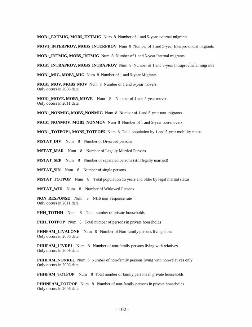
- 102 -

MOB1_EXTMIG, MOB5_EXTMIG Num 8 Number of 1 and 5-year external migrants

MOV1_INTERPROV, MOB5_INTERPROV Num 8 Number of 1 and 5-year Interprovincial migrants

MOB1_INTMIG, MOB5_INTMIG Num 8 Number of 1 and 5-year Internal migrants

MOB1_INTRAPROV, MOB5_INTRAPROV Num 8 Number of 1 and 5-year Intraprovincial migrants

MOB1_MIG, MOB5_MIG Num 8 Number of 1 and 5-year Migrants

MOB1_MOV, MOB5_MOV Num 8 Number of 1 and 5-year movers

Only occurs in 2006 data.

MOB1_MOVE, MOB5_MOVE Num 8 Number of 1 and 5-year movers

Only occurs in 2011 data.

MOB1_NONMIG, MOB5_NONMIG Num 8 Number of 1 and 5-year non-migrants

MOB1_NONMOV, MOB5_NONMOV Num 8 Number of 1 and 5-year non-movers

MOB1_TOTPOP1, MON5_TOTPOP5 Num 8 Total population by 1 and 5-year mobility status

MSTAT_DIV Num 8 Number of Divorced persons

MSTAT_MAR Num 8 Number of Legally Married Persons

MSTAT_SEP Num 8 Number of separated persons (still legally married)

MSTAT_SIN Num 8 Number of single persons

MSTAT_TOTPOP Num 8 Total population 15 years and older by legal marital status

MSTAT_WID Num 8 Number of Widowed Persons

NON_RESPONSE Num 8 NHS non_response rate

Only occurs in 2011 data.

PHH_TOTHH Num 8 Total number of private households

PHH_TOTPOP Num 8 Total number of persons in private households

PHHFAM_LIVALONE Num 8 Number of Non-family persons living alone

Only occurs in 2006 data.

PHHFAM_LIVREL Num 8 Number of non-family persons living with relatives

Only occurs in 2006 data.

PHHFAM_NONREL Num 8 Number of non-family persons living with non-relatives only

Only occurs in 2006 data.

PHHFAM_TOTPOP Num 8 Total number of family persons in private households

PHHNFAM_TOTPOP Num 8 Number of non-family persons in private households

Only occurs in 2006 data.

- 103 -

PHHNFAM_LIVALONE Num 8 Number of Non-family persons living alone

Only occurs in 2011 data.

PHHNFAM_LIVREL Num 8 Number of Non-Family persons living with relatives

Only occurs in 2011 data.

PHHNFAM_NONREL Num 8 Number of Non-Family persons living with non-relatives only

Only occurs in 2011 data.

POPFEM0004-POPFEM85 Num 8 Female population measured in 4 year intervals

POPFEM0004

POPFEM0509

POPFEM1014

POPFEM1419

POPFEM2024

POPFEM2529

POPFEM3034

POPFEM3539

POPFEM4044

POPFEM4549

POPFEM5054

POPFEM5559

POPFEM6064

POPFEM6569

POPFEM7074

POPFEM7579

POPFEM8084

POPFEM85

POPMALE0004-POPMALE85 Num 8 Male population measured in 4 year intervals

Due to an error, POPMALE3034 only occurs in 2006 data, while the corresponding variable in 2011 data is

POPMALE3039.

POPMALE0004

POPMALE0509

POPMALE1014

POPMALE1519

POPMALE2024

POPMALE2529

POPMALE3034 or POPMALE3039

POPMALE3539

POPMALE4044

POPMALE4549

POPMALE5054

POPMALE5559

POPMALE6064

POPMALE6569

POPMALE7074

POPMALE7579

POPMALE8084

POPMALE85

POPTOT Num 8 Total population

POPTOT_FEM Num 8 Total female population

POPTOT_MALE Num 8 Total male population

- 104 -

POPTOT_ROUND Num 8 Total population (Rounded)

Only occurs in 2011 data.

QUALITY Char 5

Only occurs in 2011 data.

QUALITYN Num 8

Only occurs in 2011 data.

QUALITY_NHS Char 5

Only occurs in 2011 data.

QUALITY_NHSN Num 8

Only occurs in 2011 data.

QUINT Char 2 Income Quintile (pc)

RHA Char 2 Regional Health Authority

RP Char 2 Region / Province Unique Identifier Code

Only occurs in 2006 data.

SEFI Num 8 SES Factor Index

SEX Char 1 Biological sex

WPG_CA Char 3 Winnipeg Community Areas

Prescription Drug Dictionary

This dataset is part of the MCHP SAS Course database. Use of this data must be accompanied by the

‘MCHP SAS Workshop Simulated Administrative Health Data Use Agreement’. The datasets in this

resource have been simulated using distributions of services within the Manitoba population which means

that analysis for course should be representative of services and outcomes within Manitoba over the period

2005/06 – 2013/14.

There are two supporting files that can be used with this data.

ATC_CODES – this is a list of ATC codes that can be matched by DIN.

DRUG_COST – this is a list of unit costs that can be matched by DIN.

NOTE: This data is not real and any correspondence to actual events, people or services are only

coincidental.

This simulated data represents prescriptions filled at a retail pharmacy.

These data represent 1403467 observations and 17 variables.

Name of resource: DRUG

BIRTHDT NUM 8 Birth Date (mod)

- 105 -

Date of birth from the training resource registry file. This variable is modified from the original date of

birth found in the research repository. SAS Date format variable (YYMMDD10.)

age =floor(yrdif(birthdt,dateprvd,'age'));

DAYSUPP Num 8 Days Supply on Rx

Range: -1-999

This is the number of days that the prescription fill is expected to last.

Caution: This is a mandatory field. Because of this, some caution should be used. For the 1995/96

Pharmaceutical Use project it was felt that the 0 days supply and many of the 1 days supply did not reflect

the true number of days supply. This variable most likely reflects the true days supply for scheduled

medications such as antibiotics, but most likely does not for medications which are prescribed on a prn (as

required) basis.

DIN Char 8 Drug Identification Number this claim

This is an 8 digit number assigned by the Drugs Program (Health Canada) to each drug approved for use in

Canada in accordance with the Food and Drug Regulation. Note that the same drug (e.g. Amoxicillin, 250

mg capsules) can have a number of different DINs associated with it (different manufacturers etc.). For

more information on ATC codes, refer to the concept dictionary. For more information on DIN, look at the

UPMODE and UP_DINMST data files.

DRUGCOST Num 8 Drug cost claimed

Range $0.01-$9999.99

Note some values of this field will be missing and must be imputed from the UPMODE data. It is the

amount in dollars and cents that the pharmacy is claiming for payment. However, it is not necessarily the

amount PAID by government on the claim (incostpd).

ID Char 6 Personal ID Number (Mod)

This is a personal identifier that can be used in all of the training resource data. It is NOT related to PHIN

or family registration number. This number is assigned from the training resource registry. For more

information on the individual, refer to the CENSUS2001, REGISTRY, and REGISTRY_FAMILY data

files.

INCOSTPD Num 8 16 Drug Cost paid – INGRED

Range: $0.01-$9998

This is the drug or ingredient cost approved and paid for by the program. It is used to assign ingredient cost

in expenditure/cost calculations but may adjudicated ‘downward’ based on daysupp > 100 days and/or on a

unit price (unitprc) that exceeds and expenditure validity check.

IQ Char 2 Income Quintile

Neighbourhood income quintiles based. Income quintiles have been divided into Urban (Winnipeg &

Brandon) and Rural Manitoba. The first character of the quintile indicates the location. A further division

of NF is used to identify a large group of Manitoba individuals that can not be assigned a neighbourhood

income. Most of these individuals are in institutions (PCH, Prison, LTC hospital) or covered by some form

of social services. This value is assigned from the training resource registry.

U1 Urban lowest income quintile

U2

U3

U4

U5 Urban highest income quintile

R1 Rural lowest income quintile

R2

R3

R4 Rural highest income quintile

NF Not found or not assigned

- 106 -

MQTYCLM Num 8 40 Metric Quantity claimed

Range: 0-90000

There may be a consistency problem with mqtyclm: Many drugs can be described using multiple metric

quantity descriptions. For example, a 200 mL bottle of 250 mg/5 mL amoxicillin could be described as: 1

(bottle), 200 mL, 100 g or 10,000 mg. Also, mqtyclm is the variable to use for calculation of many of the

pharmaceutical concepts as it will resemble most closely that quantity of drug actually dispensed to the

person.

PRESMDCBLOC Char 3 MH Bloc of Specialty for prescriber

PROFEEPD Num 8 24 Professional fee paid

$0-$921.95

This is the dispensing or professional approved and paid for by the program. Note for C2, the current

method of reimbursing pharmacies for providing the service is based on a capitated rate per bed exclusive

for ingredient cost.

PRVDDT Num 8 Date Provided

Range: 19990401 - 2010415

This is the date that the prescription was filled. This is a character string in the format YYMMDD8. SAS

Date format variable (YYMMDD10.)

RHA Char 2 73 Regional Health Authority

Format: $RHAL

This is the RHA that the individual was living in during the sample period. In the training resource

individuals have been assigned a single RHA for the whole period. This is NOT the case in the actual

research repository. The coding used at MCHP is not the same as Manitoba Health. ArcView Shape files

are available for mapping these areas.

MCHP Name

IE IE Interlake Eastern

IE1 Interlake Eastern Selkirk Zone

IE2 Interlake Eastern South Zone

IE3 Interlake Eastern East Zone

IE4 Interlake Eastern West Zone

IE5 Interlake Eastern North Zone

IE6 Interlake Eastern Remote Zone

NO NO Northern

NO1 Northern Direct Service Zone

NO2 Northern Non-Direct Service Zone

NO3 Northern island Lake Zone

SO SO Southern Zone

SO1 Southern North Zone

SO2 Southern Mid Zone

SO3 Southern West Zone

SO4 Southern East Zone

WE WE Prairie Mountain

WE1 PMH North Zone

WE2 PMH Brandon Zone

WE3 PMH South Zone

WP WP Winnipeg

WP11 Winnipeg Urban

WP21 Winnipeg Churchill

SEX Char 1 64 Biological gender of individual

Format: $SEXF

- 107 -

1 Male

2 Female

UNITPRC Num 8 32 Unit price paid for drug this claim

Range: $0-9998

This is the price that is approved for payment on a per mqty basis. Unitprc is a field/variable used to

validate the price of the claim.

WPG_CA Char 3 75 Winnipeg Community Areas

Format: $WPG_CAL

These are Winnipeg subregions similar in size the non-Winnipeg RHAs. Note there are a small number of

individuals with a Winnipeg RHA (K) that are not assigned to a Winnipeg Community area. These values

are assigned from the training registry. ArcView Shape files are available for mapping these areas.

W02 ASSINIBOINE SOUTH

W11 DOWNTOWN

W03 FORT GARRY

W09 INKSTER

W10 POINT DOUGLAS

W07 RIVER EAST

W12 RIVER HEIGHTS

W08 SEVEN OAKS

W04 ST. VITAL

W05 ST.BONIFACE

W01 ST.JAMES-ASSINIBOIA

W06 TRANSCONA

ATC Codes Dictionary

This dataset is part of the MCHP SAS Course database. Use of this data must be accompanied by the

‘MCHP SAS Workshop Simulated Administrative Health Data Use Agreement’. This data set may be

merged with the Course Prescription dataset by DIN.

The data represents 5139 observations and 6 variables.

Name of Resource: ATC_CODES

ATC Char 7 Anatomical Therapeutic Chemical Drug Classification System

Format: $ATCL.

ATC is a system for classifying drugs that is widely used in European countries. It is becoming more

commonly used in Canada and is managed by Health Canada. Drugs are divided into different groups

according to the organ or system on which they act and their chemical, pharmacological and therapeutic

properties. There are 5 different levels of groupings.

DDD Num 8 Defined Daily Dose

Range: 0.004-250

One of four measures of intensity of use, DDD is the assumed average maintenance dose per day for a drug

product when used for its major indication in everyday practice. This is a technical unit of measurement

and does not necessarily reflect the actual amount or dose used; it is also limited to solid drug forms only.

- 108 -

DIN Char 8 Drug Identification Number this claim

This is an 8 digit number assigned by the Drugs Program (Health Canada) to each drug approved for use in

Canada in accordance with the Food and Drug Regulation. Note that the same drug (e.g. Amoxicillin, 250

mg capsules) can have a number of different DINs associated with it (different manufacturers etc.).

PRODE Char 35 Product description in English.

PRODG Char 30 Equivalent generic production name.

STR_NEW Num 8

Range: 0.001-500

This refers to the strength, without the unit attached, but in the units of the DDD (ie. DDDUNIT). This has

been filled in for solid dosage forms, with 1 active ingredient (NAIS=1), for use in the DDD calculations.

Drug Cost Dictionary

This dataset is part of the MCHP SAS Course database. Use of this data must be accompanied by the

‘MCHP SAS Workshop Simulated Administrative Health Data Use Agreement’. The datasets in this

resource have been simulated using distributions of services within the Manitoba population which means

that analysis for course should be representative of services and outcomes within Manitoba. This dataset

may be merged with the Course Prescription dataset by DIN. Not every record in the prescription file

contains an associated unit cost this data set will allow you to add an estimated unit cost value. The datasets

in this resource have been simulated using distributions of services within the Manitoba population which

means that analysis for course should be representative of services and outcomes within Manitoba over the

period 2005/06 – 2013/14.

The data represents 5451 observations and 14 variables.

Name of resource: UPMODE

DIN Char 8 Drug Identification Number this claim

This is an 8 digit number assigned by the Drugs Program (Health Canada) to each drug approved for use in

Canada in accordance with the Food and Drug Regulation. Note that the same drug (e.g. Amoxicillin, 250

mg capsules) can have a number of different DINs associated with it (different manufacturers etc.).

P50 Num 8 the median, MQTYPAID

P75 Num 8 the upper quartile, MQTYPAID

P90 Num 8 the 90th percentile, MQTYPAID

P95 Num 8 the 95th percentile, MQTYPAID

QTYMODE Num 8 the most frequent value, MQTYPAID

QTYN Num 8 number of nonmissing values, MQTYPAID

UPMAX Num 8 the largest value, UNITPRC

UPMEAN Num 8 the mean, UNITPRC

UPMED Num 8 the median, UNITPRC

- 109 -

UPMIN Num 8 the smallest value, UNITPRC

UPMODE Num 8 the most frequent value, UNITPRC

UPN Num 8 number of nonmissing values, UNITPRC

UPSTD Num 8 the standard deviation, UNITPRC

Provided SAS Macro Code

The following SAS macros have been provided for use with MCHP workshop data. In most cases

documentation for using the macro is either provided in a separate .docs file or at the top of the provided

SAS code. Examples of the three most commonly used macros have been provided below.

Macro Names:

_age – Correctly calculate age using intck function instead of yrdif.

_charlsonicd10 – Generate Charlson Comorbidity Scores for hospital separations

_dumvar – Create Dummy variables based on values in a categorical variable.

_elixhausericd10 - Generate Elixhauser Scores for hospital separations

_extlog – Extract SAS code from a SAS log file

_icd10l – Create labels for ICD10 or CCI codes. This macro assumes that the data provided for the

course is in a library called ‘COURSE’. There is an option to use a different library name if

necessary.

_lotus – Write out delimited text files

pop_rate.sas – Calculate age/sex direct or indirect adjusted rates

_random – Select random samples from a dataset

fixday – Correct invalid date strings (e.g. 20040229).

Examples:

Example for adding Charlson Comorbidity Score based on work by Hude Quan, 2005 libname course 'X:\course\Data' ;

*** Include macro code for calculating index ;

%include 'X:\course\macros\_charlsonicd10.sas' ;

data test ;

set course.hospital ;

run ;

*** Add comorbidity information to a new output dataset called cmb_out;

%_charlsonicd10(data=test, out=cmb_out, dx=icd10_01-icd10_10,

type=off) ;

Quan H, Sundararajan V, Halfon P, Fong A, Burnand B, Luthi JC, Saunders LD, Beck CA, Feasby TE,

Ghali WA. Coding algorithms for defining comorbidities in ICD-9-CM and ICD-10 administrative data.

Med Care 2005;43(11):1130-1139.

Example for adding ICD10CA or CCI Labels to your output.

*** Include macro code for creating labels;

%include 'X:\course\macros\_icd10l.sas' ;

*** Generate ICD10CA labels ;

%_icd10l(fmt=icd10,syear=2004) ;

proc freq data=test ;

tables icd10_01 ;

format icd10_01 $icd1004l. ;

run ;

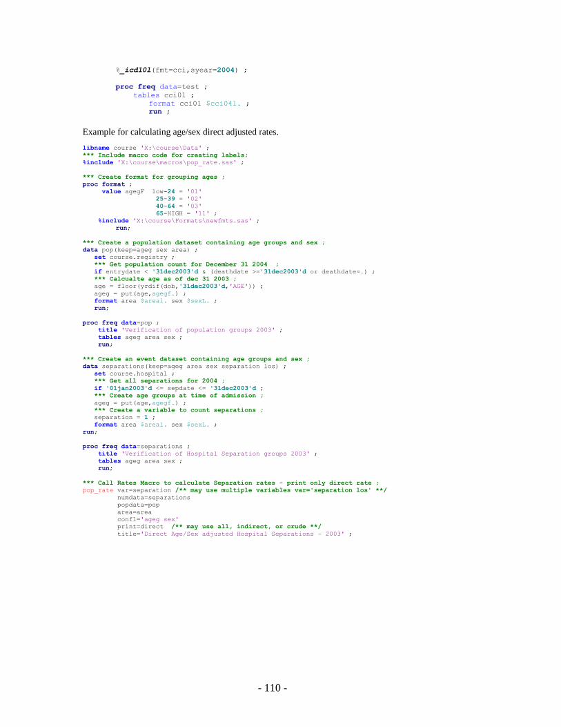
- 110 -

%_icd10l(fmt=cci,syear=2004) ;

proc freq data=test ;

tables cci01 ;

format cci01 $cci04l. ;

run ;

Example for calculating age/sex direct adjusted rates.

libname course 'X:\course\Data' ;

*** Include macro code for creating labels;

%include 'X:\course\macros\pop_rate.sas' ;

*** Create format for grouping ages ;

proc format ;

value agegF low-24 = '01'

25-39 = '02'

40-64 = '03'

65-HIGH = '11' ;

%include 'X:\course\Formats\newfmts.sas' ;

run;

*** Create a population dataset containing age groups and sex ;

data pop(keep=ageg sex area) ;

set course.registry ;

*** Get population count for December 31 2004 ;

if entrydate < '31dec2003'd & (deathdate >='31dec2003'd or deathdate=.) ;

*** Calcualte age as of dec 31 2003 ;

age = floor(yrdif(dob,'31dec2003'd,'AGE')) ;

ageg = put(age,agegf.) ;

format area $areal. sex $sexL. ;

run;

proc freq data=pop ;

title 'Verification of population groups 2003' ;

tables ageg area sex ;

run;

*** Create an event dataset containing age groups and sex ;

data separations(keep=ageg area sex separation los) ;

set course.hospital ;

*** Get all separations for 2004 ;

if '01jan2003'd <= sepdate <= '31dec2003'd ;

*** Create age groups at time of admission ;

ageg = put(age,agegf.) ;

*** Create a variable to count separations ;

separation = 1 ;

format area $areal. sex $sexL. ;

run;

proc freq data=separations ;

title 'Verification of Hospital Separation groups 2003' ;

tables ageg area sex ;

run;

*** Call Rates Macro to calculate Separation rates - print only direct rate ;

pop_rate var=separation /** may use multiple variables var='separation los' **/

numdata=separations

popdata=pop

area=area

conf1='ageg sex'

print=direct /** may use all, indirect, or crude **/

title='Direct Age/Sex adjusted Hospital Separations - 2003' ;

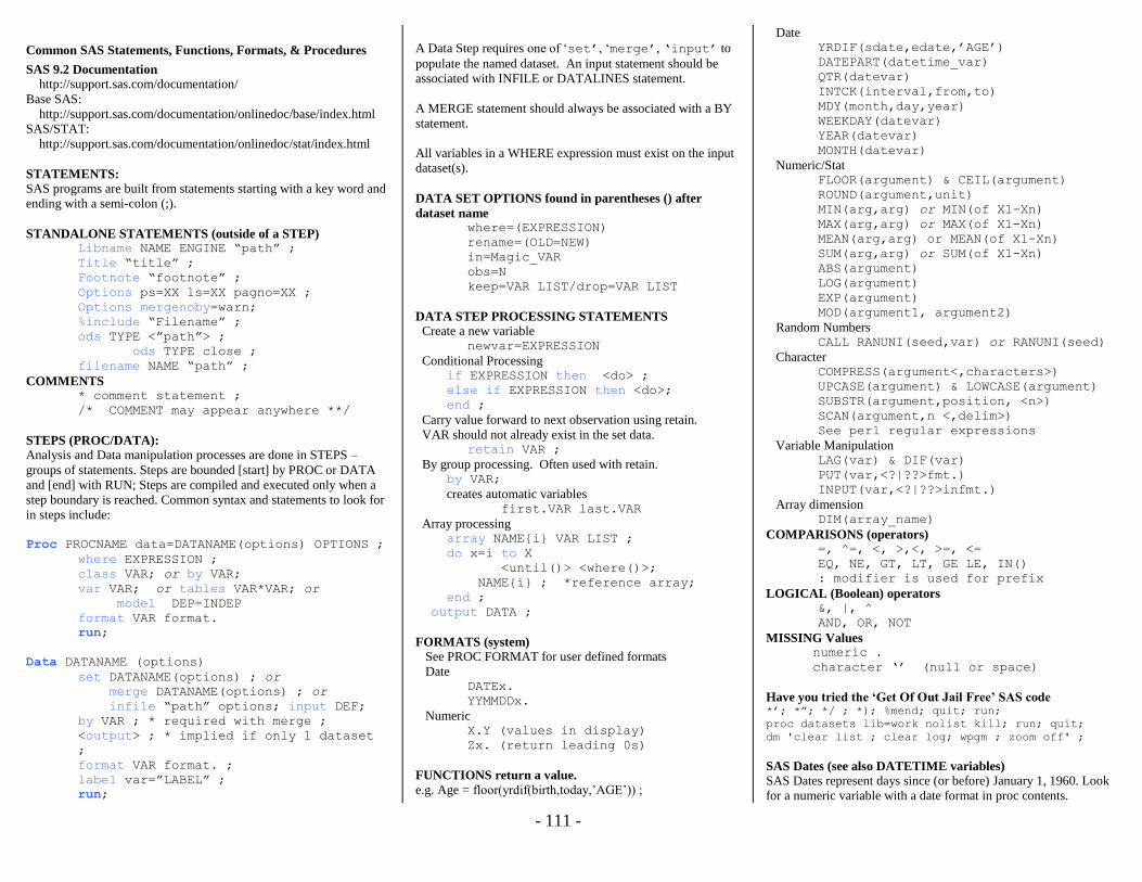
- 111 -

Common SAS Statements, Functions, Formats, & Procedures

SAS 9.2 Documentation

http://support.sas.com/documentation/

Base SAS:

http://support.sas.com/documentation/onlinedoc/base/index.html

SAS/STAT:

http://support.sas.com/documentation/onlinedoc/stat/index.html

STATEMENTS:

SAS programs are built from statements starting with a key word and

ending with a semi-colon (;).

STANDALONE STATEMENTS (outside of a STEP) Libname NAME ENGINE “path” ;

Title “title” ;

Footnote “footnote” ;

Options ps=XX ls=XX pagno=XX ;

Options mergenoby=warn;

%include “Filename” ;

ods TYPE <”path”> ;

ods TYPE close ;

filename NAME “path” ;

COMMENTS * comment statement ;

/* COMMENT may appear anywhere **/

STEPS (PROC/DATA):

Analysis and Data manipulation processes are done in STEPS –

groups of statements. Steps are bounded [start] by PROC or DATA

and [end] with RUN; Steps are compiled and executed only when a

step boundary is reached. Common syntax and statements to look for

in steps include:

Proc PROCNAME data=DATANAME(options) OPTIONS ;

where EXPRESSION ;

class VAR; or by VAR;

var VAR; or tables VAR*VAR; or

model DEP=INDEP

format VAR format.

run;

Data DATANAME (options)

set DATANAME(options) ; or

merge DATANAME(options) ; or

infile “path” options; input DEF;

by VAR ; * required with merge ;

<output> ; * implied if only 1 dataset

;

format VAR format. ;

label var=”LABEL” ;

run;

A Data Step requires one of ‘set’, ‘merge’, ‘input’ to

populate the named dataset. An input statement should be

associated with INFILE or DATALINES statement.

A MERGE statement should always be associated with a BY

statement.

All variables in a WHERE expression must exist on the input

dataset(s).

DATA SET OPTIONS found in parentheses () after

dataset name where=(EXPRESSION)

rename=(OLD=NEW)

in=Magic_VAR

obs=N

keep=VAR LIST/drop=VAR LIST

DATA STEP PROCESSING STATEMENTS

Create a new variable newvar=EXPRESSION

Conditional Processing if EXPRESSION then <do> ;

else if EXPRESSION then <do>;

end ;

Carry value forward to next observation using retain.

VAR should not already exist in the set data. retain VAR ;

By group processing. Often used with retain. by VAR;

creates automatic variables first.VAR last.VAR

Array processing array NAME{i} VAR LIST ;

do x=i to X

<until()> <where()>;

NAME{i} ; *reference array;

end ;

output DATA ;

FORMATS (system)

See PROC FORMAT for user defined formats

Date DATEx.

YYMMDDx.

Numeric X.Y (values in display)

Zx. (return leading 0s)

FUNCTIONS return a value.

e.g. Age = floor(yrdif(birth,today,’AGE’)) ;

Date YRDIF(sdate,edate,’AGE’)

DATEPART(datetime_var)

QTR(datevar)

INTCK(interval,from,to)

MDY(month,day,year)

WEEKDAY(datevar)

YEAR(datevar)

MONTH(datevar)

Numeric/Stat FLOOR(argument) & CEIL(argument)

ROUND(argument,unit)

MIN(arg,arg) or MIN(of X1-Xn)

MAX(arg,arg) or MAX(of X1-Xn)

MEAN(arg,arg) or MEAN(of X1-Xn)

SUM(arg,arg) or SUM(of X1-Xn)

ABS(argument)

LOG(argument)

EXP(argument)

MOD(argument1, argument2)

Random Numbers CALL RANUNI(seed,var) or RANUNI(seed)

Character COMPRESS(argument<,characters>)

UPCASE(argument) & LOWCASE(argument)

SUBSTR(argument,position, <n>)

SCAN(argument,n <,delim>)

See perl regular expressions

Variable Manipulation LAG(var) & DIF(var)

PUT(var,<?|??>fmt.)

INPUT(var,<?|??>infmt.)

Array dimension DIM(array_name)

COMPARISONS (operators) =, ^=, <, >,<, >=, <=

EQ, NE, GT, LT, GE LE, IN()

: modifier is used for prefix

LOGICAL (Boolean) operators &, |, ^

AND, OR, NOT

MISSING Values numeric .

character ‘’ (null or space)

Have you tried the ‘Get Of Out Jail Free’ SAS code *’; *”; */ ; *); %mend; quit; run;

proc datasets lib=work nolist kill; run; quit;

dm 'clear list ; clear log; wpgm ; zoom off' ;

SAS Dates (see also DATETIME variables) SAS Dates represent days since (or before) January 1, 1960. Look

for a numeric variable with a date format in proc contents.

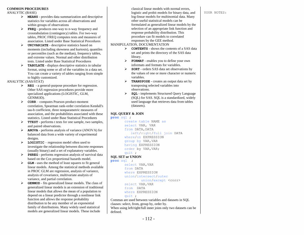
- 112 -

COMMON PROCEDURES

ANALYTIC (BASE)

MEANS - provides data summarization and descriptive

statistics for variables across all observations and

within groups of observations

FREQ - produces one-way to n-way frequency and

crosstabulation (contingency) tables. For two-way

tables, PROC FREQ computes tests and measures of

association. Listed under Base Statistical Procedures

UNIVARIATE - descriptive statistics based on

moments (including skewness and kurtosis), quantiles

or percentiles (such as the median), frequency tables,

and extreme values. Normal and other distribution

tests. Listed under Base Statistical Procedures

TABULATE - displays descriptive statistics in tabular

format, using some or all of the variables in a data set.

You can create a variety of tables ranging from simple

to highly customized.

ANALYTIC (SAS/STAT)

REG - a general-purpose procedure for regression.

Other SAS regression procedures provide more

specialized applications (LOGISTIC, GLM,

GENMOD).

CORR – computes Pearson product-moment

correlation, Spearman rank-order correlation Kendall's

tau-b coefficient, three nonparametric measures of

association, and the probabilities associated with these

statistics. Listed under Base Statistical Procedures

TTEST - performs t tests for one sample, two samples,

and paired observations.

ANOVA - performs analysis of variance (ANOVA) for

balanced data from a wide variety of experimental

designs.

LOGISTIC – regression model often used to

investigate the relationship between discrete responses

(usually binary) and a set of explanatory variables.

PHREG - performs regression analysis of survival data

based on the Cox proportional hazards model.

GLM - uses the method of least squares to fit general

linear models. Among the statistical methods available

in PROC GLM are regression, analysis of variance,

analysis of covariance, multivariate analysis of

variance, and partial correlation.

GENMOD - fits generalized linear models. The class of

generalized linear models is an extension of traditional

linear models that allows the mean of a population to

depend on a linear predictor through a nonlinear link

function and allows the response probability

distribution to be any member of an exponential

family of distributions. Many widely used statistical

models are generalized linear models. These include

classical linear models with normal errors,

logistic and probit models for binary data, and

log-linear models for multinomial data. Many

other useful statistical models can be

formulated as generalized linear models by the

selection of an appropriate link function and

response probability distribution. This

procedure can fit models to correlated

responses by the GEE method.

MANIPULATION, DOCUMENTATION

CONTENTS - shows the contents of a SAS data

set and prints the directory of the SAS data

library.

FORMAT - enables you to define your own

informats and formats for variables.

SORT - orders SAS data set observations by

the values of one or more character or numeric

variables.

TRANSPOSE - creates an output data set by

transposing selected variables into

observations.

SQL - implements Structured Query Language

(SQL) for SAS. SQL is a standardized, widely

used language that retrieves data from tables

(datasets).

SQL QUERY & JOIN proc sql ;

create table NAME as

select VAR, VAR

from DATA,DATA

left/right/full join DATA

where/on EXPRESSION

group by VAR,VAR

having EXPRESSION

order by VAR,VAR;

quit ;

SQL SET or UNION proc sql ;

select VAR,VAR

from DATA

where EXPRESSION

union/intersect/outer

union/except <corr>

select VAR,VAR

from DATA

where EXPRESSION

quit ;

Commas are used between variables and datasets in SQL

clauses: select, from, group by, order by.

When using left/right/full inner joins only two datasets can be

defined.

YOUR NOTES: