sas/stat 9.2 user's guide: shared concepts and topics

SAS/STAT® 9.2 User’s GuideShared Concepts and Topics(Book Excerpt)

SAS® Documentation

This document is an individual chapter from SAS/STAT® 9.2 User’s Guide.

The correct bibliographic citation for the complete manual is as follows: SAS Institute Inc. 2008. SAS/STAT® 9.2User’s Guide. Cary, NC: SAS Institute Inc.

Copyright © 2008, SAS Institute Inc., Cary, NC, USA

All rights reserved. Produced in the United States of America.

For a Web download or e-book: Your use of this publication shall be governed by the terms established by the vendorat the time you acquire this publication.

U.S. Government Restricted Rights Notice: Use, duplication, or disclosure of this software and related documentationby the U.S. government is subject to the Agreement with SAS Institute and the restrictions set forth in FAR 52.227-19,Commercial Computer Software-Restricted Rights (June 1987).

SAS Institute Inc., SAS Campus Drive, Cary, North Carolina 27513.

1st electronic book, March 20082nd electronic book, February 2009SAS® Publishing provides a complete selection of books and electronic products to help customers use SAS software toits fullest potential. For more information about our e-books, e-learning products, CDs, and hard-copy books, visit theSAS Publishing Web site at support.sas.com/publishing or call 1-800-727-3228.

SAS® and all other SAS Institute Inc. product or service names are registered trademarks or trademarks of SAS InstituteInc. in the USA and other countries. ® indicates USA registration.

Other brand and product names are registered trademarks or trademarks of their respective companies.

Chapter 18

Shared Concepts and Topics

ContentsLevelization of Classification Variables . . . . . . . . . . . . . . . . . . . . . . . 366Parameterization of Model Effects . . . . . . . . . . . . . . . . . . . . . . . . . . 368

GLM Parameterization of Classification Variables and Effects . . . . . . . . 369Intercept . . . . . . . . . . . . . . . . . . . . . . . . . . . . . . . . 369Regression Effects . . . . . . . . . . . . . . . . . . . . . . . . . . 369Main Effects . . . . . . . . . . . . . . . . . . . . . . . . . . . . . 369Interaction Effects . . . . . . . . . . . . . . . . . . . . . . . . . . 370Nested Effects . . . . . . . . . . . . . . . . . . . . . . . . . . . . . 371Continuous-Nesting-Class Effects . . . . . . . . . . . . . . . . . . 371Continuous-by-Class Effects . . . . . . . . . . . . . . . . . . . . . 372General Effects . . . . . . . . . . . . . . . . . . . . . . . . . . . . 372

Other Parameterizations . . . . . . . . . . . . . . . . . . . . . . . . . . . . 373Constructed Effects and the EFFECT Statement (Experimental) . . . . . . . . . . 377

Collection Effects . . . . . . . . . . . . . . . . . . . . . . . . . . . . . . . 378Multimember Effects . . . . . . . . . . . . . . . . . . . . . . . . . . . . . . 378Polynomial Effects . . . . . . . . . . . . . . . . . . . . . . . . . . . . . . . 380Spline Effects . . . . . . . . . . . . . . . . . . . . . . . . . . . . . . . . . 384Splines and Spline Bases . . . . . . . . . . . . . . . . . . . . . . . . . . . . 387

Truncated Power Function Basis . . . . . . . . . . . . . . . . . . . 388B-Spline Basis . . . . . . . . . . . . . . . . . . . . . . . . . . . . 389

Nonlinear Optimization: The NLOPTIONS Statement . . . . . . . . . . . . . . . 391Syntax . . . . . . . . . . . . . . . . . . . . . . . . . . . . . . . . . . . . . 391Remote Monitoring . . . . . . . . . . . . . . . . . . . . . . . . . . . . . . 403Choosing an Optimization Algorithm . . . . . . . . . . . . . . . . . . . . . 405

First- or Second-Order Algorithms . . . . . . . . . . . . . . . . . . 405Algorithm Descriptions . . . . . . . . . . . . . . . . . . . . . . . . 406

Programming Statements . . . . . . . . . . . . . . . . . . . . . . . . . . . . . . . 410References . . . . . . . . . . . . . . . . . . . . . . . . . . . . . . . . . . . . . . 412

366 F Chapter 18: Shared Concepts and Topics

This chapter introduces a number of concepts that are common to one or more procedures inSAS/STAT, such as the parameterization of effects, the use of the experimental EFFECT state-ment, and so on. The beginning of each major section displays a listing of the procedures for whichthe shared topic is relevant.

Levelization of Classification Variables

A classification variable is a variable that enters the statistical analysis or model not through itsvalues, but through its levels. The process of associating values of a variable with levels is termedlevelization.

A sufficient, but not necessary, condition for a procedure to perform levelization of classificationvariables is the presence of a CLASS statement. Hence, this section applies to all SAS/STATprocedures that support a CLASS statement. Some procedures use different syntax elements torequest levelization of variables (for example, the TRANSREG procedure).

During the process of levelization, observations that share the same value are assigned to the samelevel. The manner in which values are grouped can be affected by the inclusion of formats. The sortorder of the levels can be determined with the ORDER= option in the procedure statement. Withthe GENMOD, GLMSELECT, and LOGISTIC procedures, you can also control the sorting orderseparately for each variable in the CLASS statement.

Consider the data on nine observations in Table 18.1. The variable A is integer valued, and variableX is a continuous variable with a missing value for the fourth observations. The fourth and fifthcolumns of Table 18.1 apply two different formats to the variable X.

Table 18.1 Example Data for Levelization

Obs A x formatx 3.0

formatx 3.1

1 1 1.09 1 1.12 1 1.13 1 1.13 1 1.27 1 1.34 2 . . .5 2 2.26 2 2.36 2 2.48 2 2.57 3 3.34 3 3.38 3 3.34 3 3.39 3 3.14 3 3.1

By default, levelization of the variables groups observations by the formatted value of the variable,except for numerical variables where no explicit format is provided. These are sorted by theirinternal value. The levelization of the four columns in table Table 18.1 leads to the level assignmentin Table 18.2.

Levelization of Classification Variables F 367

Table 18.2 Values and Levels

A X format x 3.0 format x 3.1Obs Value Level Value Level Value Level Value Level

1 2 1 1.09 1 1 1 1.1 12 2 1 1.13 2 1 1 1.1 13 2 1 1.27 3 1 1 1.3 24 3 2 . . . . . .5 3 2 2.26 4 2 2 2.3 36 3 2 2.48 5 2 2 2.5 47 4 3 3.34 7 3 3 3.3 68 4 3 3.34 7 3 3 3.3 69 4 3 3.14 6 3 3 3.1 5

The ORDER= option in the PROC statement specifies the sorting order for the levels of CLASSvariables. When the default ORDER=FORMATTED is in effect for numeric variables for whichyou have supplied no explicit format, the levels are ordered by their internal values. To ordernumeric class levels with no explicit format by their BEST12. formatted values, you can specifythis format explicitly for the CLASS variables.

The following table shows how values of the ORDER= option are interpreted.

Value of ORDER= Levels Sorted By

DATA order of appearance in the input data set

FORMATTED external formatted value, except for numeric variableswith no explicit format, which are sorted by their unfor-matted (internal) value

FREQ descending frequency count; levels with the most obser-vations come first in the order

INTERNAL unformatted value

For FORMATTED and INTERNAL values, the sort order is machine dependent. For more infor-mation about sort order, see the chapter on the SORT procedure in the Base SAS Procedures Guideand the discussion of BY-group processing in SAS Language Reference: Concepts.

The GLMSELECT, LOGISTIC, and GENMOD procedures support a MISSING option in theCLASS statement. When this option is in effect, missing values (‘.’ for a numeric variable andblanks for a character variable) are included in the levelization and are assigned a level. Table 18.3displays the results of levelizing the values in Table 18.1 when the MISSING option is in effect.


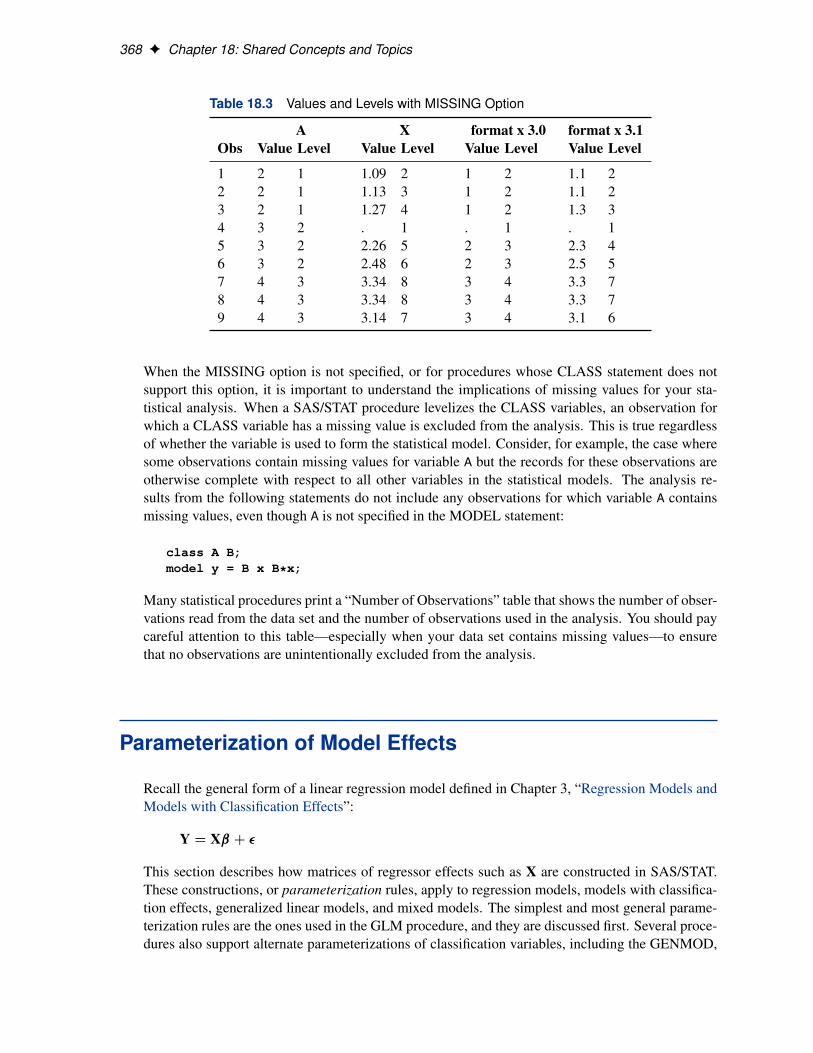
Table 18.3 Values and Levels with MISSING Option

A X format x 3.0 format x 3.1Obs Value Level Value Level Value Level Value Level

1 2 1 1.09 2 1 2 1.1 22 2 1 1.13 3 1 2 1.1 23 2 1 1.27 4 1 2 1.3 34 3 2 . 1 . 1 . 15 3 2 2.26 5 2 3 2.3 46 3 2 2.48 6 2 3 2.5 57 4 3 3.34 8 3 4 3.3 78 4 3 3.34 8 3 4 3.3 79 4 3 3.14 7 3 4 3.1 6

When the MISSING option is not specified, or for procedures whose CLASS statement does notsupport this option, it is important to understand the implications of missing values for your sta-tistical analysis. When a SAS/STAT procedure levelizes the CLASS variables, an observation forwhich a CLASS variable has a missing value is excluded from the analysis. This is true regardlessof whether the variable is used to form the statistical model. Consider, for example, the case wheresome observations contain missing values for variable A but the records for these observations areotherwise complete with respect to all other variables in the statistical models. The analysis re-sults from the following statements do not include any observations for which variable A containsmissing values, even though A is not specified in the MODEL statement:

class A B;model y = B x B*x;

Many statistical procedures print a “Number of Observations” table that shows the number of obser-vations read from the data set and the number of observations used in the analysis. You should paycareful attention to this table—especially when your data set contains missing values—to ensurethat no observations are unintentionally excluded from the analysis.

Parameterization of Model Effects

Recall the general form of a linear regression model defined in Chapter 3, “Regression Models andModels with Classification Effects”:

Y D Xˇ C �

This section describes how matrices of regressor effects such as X are constructed in SAS/STAT.These constructions, or parameterization rules, apply to regression models, models with classifica-tion effects, generalized linear models, and mixed models. The simplest and most general parame-terization rules are the ones used in the GLM procedure, and they are discussed first. Several proce-dures also support alternate parameterizations of classification variables, including the GENMOD,

GLM Parameterization of Classification Variables and Effects F 369

GLMSELECT, LOGISTIC, SURVEYLOGISTIC, and PHREG procedures. These are discussedafter the GLM parameterization of classification variables and model effects.

All modeling procedures that support classification variables and effects have a CLASS statement.Procedures that additionally support the supplemental parameterizations have a PARAM= option inthe CLASS statement.

GLM Parameterization of Classification Variables and Effects

This section applies to the following procedures:GAM, GENMOD, GLIMMIX, GLM, GLMPOWER, GLMSELECT, LIFEREG, LOGISTIC, MI,MIXED, MULLTEST, ORTHOREG, PHREG, PLS, QUANTREG, ROBUSTREG, and SURVEY-LOGISTIC.

Intercept

By default, linear models in SAS/STAT automatically include a column of 1s in X correspondingto an intercept parameter. In many procedures you can use the NOINT option in the MODELstatement to suppress this intercept. The NOINT option is useful, for example, when the MODELstatement contains a classification effect and you want the parameter estimates to be in terms of themean response for each level of that effect.

Regression Effects

Numeric variables, or polynomial terms involving them, can be included in the model as regressioneffects (covariates). The actual values of such terms are included as columns of the relevant modelmatrices. You can use the bar operator with a regression effect to generate polynomial effects. Forinstance, X|X|X expands to X X*X X*X*X, a cubic model.

Main Effects

If a classification variable has m levels, the GLM parameterization generates m columns for itsmain effect in the model matrix. Each column is an indicator variable for a given level. The orderof the columns is the sort order of the values of their levels and frequently can be controlled withthe ORDER= option in the procedure or CLASS statement.

Table 18.4 is an example where ˇ0 denotes the intercept and A and B are classification variableswith two and three levels, respectively.


Table 18.4 Example of Main Effects

Data I A B

A B ˇ0 A1 A2 B1 B2 B31 1 1 1 0 1 0 01 2 1 1 0 0 1 01 3 1 1 0 0 0 12 1 1 0 1 1 0 02 2 1 0 1 0 1 02 3 1 0 1 0 0 1

Typically, there are more columns for these effects than there are degrees of freedom to estimatethem. In other words, the GLM parameterization of main effects is singular.

Interaction Effects

Often a model includes interaction (crossed) effects to account for how the effect of a variablechanges with the values of other variables. With an interaction, the terms are first reordered tocorrespond to the order of the variables in the CLASS statement. Thus, B*A becomes A*B if Aprecedes B in the CLASS statement. Then, the GLM parameterization generates columns for allcombinations of levels that occur in the data. The order of the columns is such that the rightmostvariables in the interaction change faster than the leftmost variables (Table 18.5). Note that in theMIXED and GLIMMIX procedures, which support both fixed- and random-effects models, emptycolumns (that is, columns that would contain all 0s) are not generated for fixed effects, but they aregenerated for random effects.

Table 18.5 Example of Interaction Effects

Data I A B A*B

A B ˇ0 A1 A2 B1 B2 B3 A1B1 A1B2 A1B3 A2B1 A2B2 A2B31 1 1 1 0 1 0 0 1 0 0 0 0 01 2 1 1 0 0 1 0 0 1 0 0 0 01 3 1 1 0 0 0 1 0 0 1 0 0 02 1 1 0 1 1 0 0 0 0 0 1 0 02 2 1 0 1 0 1 0 0 0 0 0 1 02 3 1 0 1 0 0 1 0 0 0 0 0 1

In the preceding matrix, main-effects columns are not linearly independent of crossed-effectscolumns; in fact, the column space for the crossed effects contains the space of the main effect.

When your model contains many interaction effects, you might be able to code them more parsi-moniously by using the bar operator ( | ). The bar operator generates all possible interaction effects.For example, A|B|C expands to A B A*B C A*C B*C A*B*C. To eliminate higher-order interactioneffects, use the at sign (@) in conjunction with the bar operator. For instance, A|B|C|D@2 expandsto A B A*B C A*C B*C D A*D B*D C*D.

GLM Parameterization of Classification Variables and Effects F 371

Nested Effects

Nested effects are generated in the same manner as crossed effects. Hence, the design columns gen-erated by the following two statements are the same (but the ordering of the columns is different):

model Y=A B(A);

model Y=A A*B;

The nesting operator in SAS/STAT software is more of a notational convenience than an operationdistinct from crossing. Nested effects are typically characterized by the property that the nestedvariables never appear as main effects. The order of the variables within nesting parentheses is madeto correspond to the order of these variables in the CLASS statement. The order of the columns issuch that variables outside the parentheses index faster than those inside the parentheses, and therightmost nested variables index faster than the leftmost variables (Table 18.6).

Table 18.6 Example of Nested Effects

Data I A B(A)

A B ˇ0 A1 A2 B1A1 B2A1 B3A1 B1A2 B2A2 B3A21 1 1 1 0 1 0 0 0 0 01 2 1 1 0 0 1 0 0 0 01 3 1 1 0 0 0 1 0 0 02 1 1 0 1 0 0 0 1 0 02 2 1 0 1 0 0 0 0 1 02 3 1 0 1 0 0 0 0 0 1

Continuous-Nesting-Class Effects

When a continuous variable nests or crosses with a classification variable, the design columns areconstructed by multiplying the continuous values into the design columns for the classificationeffect (Table 18.7).

Table 18.7 Example of Continuous-Nesting-Class Effects

Data I A X(A)

X A ˇ0 A1 A2 X(A1) X(A2)21 1 1 1 0 21 024 1 1 1 0 24 022 1 1 1 0 22 028 2 1 0 1 0 2819 2 1 0 1 0 1923 2 1 0 1 0 23

This model estimates a separate intercept and a separate slope for X within each level of A.


Continuous-by-Class Effects

Continuous-by-class effects generate the same design columns as continuous-nesting-class effects.Table 18.8 shows the construction of the X*A effect. The two columns for this effect are the sameas the columns for the X(A) effect in Table 18.7.

Table 18.8 Example of Continuous-by-Class Effects

Data I X A X*A

X A ˇ0 X A1 A2 X*A1 X*A221 1 1 21 1 0 21 024 1 1 24 1 0 24 022 1 1 22 1 0 22 028 2 1 28 0 1 0 2819 2 1 19 0 1 0 1923 2 1 23 0 1 0 23

You can use continuous-by-class effects together with pure continuous effects to test for homogene-ity of slopes.

General Effects

An example that combines all the effects is X1*X2*A*B*C(D E). The continuous list comes first,followed by the crossed list, followed by the nested list in parentheses. You should be aware of thesequencing of parameters when you use statements that depend on the ordering of parameters, suchas the CONTRAST or ESTIMATE statements in a number of procedures, used to estimate and testfunctions of the parameter.

Effects might be renamed by the procedure to correspond to ordering rules. For example, B*A(E D)might be renamed A*B(D E) to satisfy the following:

� Classification variables that occur outside parentheses (crossed effects) are sorted in the orderin which they appear in the CLASS statement.

� Variables within parentheses (nested effects) are sorted in the order in which they appear inthe CLASS statement.

The sequencing of the parameters generated by an effect can be described by which variables havetheir levels indexed faster:

� Variables in the crossed list index faster than variables in the nested list.

� Within a crossed or nested list, variables to the right index faster than variables to the left.

For example, suppose a model includes four effects—A, B, C, and D—each having two levels, 1 and2. If the CLASS statement is

Other Parameterizations F 373

class A B C D;

then the order of the parameters for the effect B*A(C D), which is renamedA*B(C D), is

A1B1C1D1 ! A1B2C1D1 ! A2B1C1D1 ! A2B2C1D1 !



A1B1C2D2 ! A1B2C2D2 ! A2B1C2D2 ! A2B2C2D2

Note that first the crossed effects B and A are sorted in the order in which they appear in the CLASSstatement so that A precedes B in the parameter list. Then, for each combination of the nested effectsin turn, combinations of A and B appear. The B effect changes fastest because it is rightmost in thecross list. Then A changes next fastest, and D changes next fastest. The C effect changes slowestbecause it is leftmost in the nested list.

Other Parameterizations

This section applies to the following procedures:GENMOD, GLMSELECT, LOGISTIC, and PHREG.

Some SAS/STAT procedures, including GENMOD, GLMSELECT, and LOGISTIC, support non-singular parameterizations for classification effects. A variety of these nonsingular parameteriza-tions are available. In these procedures you use the PARAM= option in the CLASS statement tospecify the parameterization.

Consider a model with one CLASS variable A that has four levels, 1, 2, 5, and 7. Details of thepossible choices for the PARAM= option follow.

EFFECT Three columns are created to indicate group membership of the nonreferencelevels. For the reference level, all three dummy variables have a value of �1.For instance, if the reference level is 7 (REF=7), the design matrix columnsfor A are as follows.

Effect CodingDesign Matrix

A A1 A2 A5

1 1 0 0

2 0 1 0

5 0 0 1

7 �1 �1 �1

Parameter estimates of CLASS main effects that use the effect codingscheme estimate the difference in the effect of each nonreference level com-pared to the average effect over all four levels.


Note that the EFFECT parameterization is the default parameterization in theCATMOD procedure. See the section “Generation of the Design Matrix” onpage 1153, in Chapter 28, “The CATMOD Procedure,” for further detailsabout parameterization of model effects with the CATMOD procedure.

GLM As in the GLM procedure, four columns are created to indicate group mem-bership. The design matrix columns for A are as follows.

GLM CodingDesign Matrix

A A1 A2 A5 A7

1 1 0 0 0

2 0 1 0 0

5 0 0 1 0

7 0 0 0 1

Parameter estimates of CLASS main effects that use the GLM codingscheme estimate the difference in the effects of each level compared to thelast level. See the previous section for details about the GLM parameteriza-tion of model effects.

ORDINAL

THERMOMETER Three columns are created to indicate group membership of the higher levelsof the effect. For the first level of the effect (which for A is 1), all threedummy variables have a value of 0. The design matrix columns for A are asfollows.

Ordinal CodingDesign Matrix

A A2 A5 A7

1 0 0 0

2 1 0 0

5 1 1 0

7 1 1 1

The first level of the effect is a control or baseline level. Parameter estimatesof CLASS main effects, using the ORDINAL coding scheme, estimate thedifferences between effects of successive levels. When the parameters havethe same sign, the effect is monotonic across the levels.

POLYNOMIAL

POLY Three columns are created. The first represents the linear term .x/), thesecond represents the quadratic term

�x2

�, and the third represents the cubic

term�x3

�, where x is the level value. If the CLASS levels are not numeric,

they are translated into 1, 2, 3, : : : according to their sorting order. Thedesign matrix columns for A are as follows.

Other Parameterizations F 375

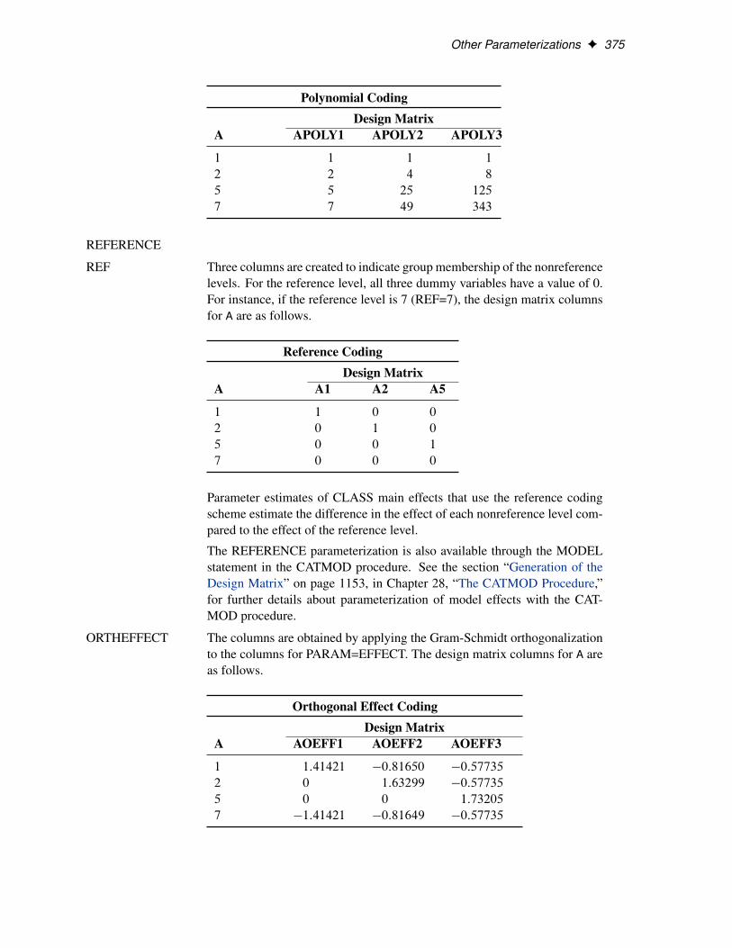
Polynomial CodingDesign Matrix

A APOLY1 APOLY2 APOLY3

1 1 1 1

2 2 4 8

5 5 25 125

7 7 49 343

REFERENCE

REF Three columns are created to indicate group membership of the nonreferencelevels. For the reference level, all three dummy variables have a value of 0.For instance, if the reference level is 7 (REF=7), the design matrix columnsfor A are as follows.

Reference CodingDesign Matrix

A A1 A2 A5

1 1 0 0

2 0 1 0

5 0 0 1

7 0 0 0

Parameter estimates of CLASS main effects that use the reference codingscheme estimate the difference in the effect of each nonreference level com-pared to the effect of the reference level.

The REFERENCE parameterization is also available through the MODELstatement in the CATMOD procedure. See the section “Generation of theDesign Matrix” on page 1153, in Chapter 28, “The CATMOD Procedure,”for further details about parameterization of model effects with the CAT-MOD procedure.

ORTHEFFECT The columns are obtained by applying the Gram-Schmidt orthogonalizationto the columns for PARAM=EFFECT. The design matrix columns for A areas follows.

Orthogonal Effect CodingDesign Matrix

A AOEFF1 AOEFF2 AOEFF3

1 1:41421 �0:81650 �0:57735

2 0 1:63299 �0:57735

5 0 0 1:73205

7 �1:41421 �0:81649 �0:57735


ORTHORDINAL

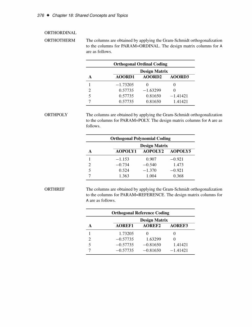
ORTHOTHERM The columns are obtained by applying the Gram-Schmidt orthogonalizationto the columns for PARAM=ORDINAL. The design matrix columns for Aare as follows.

Orthogonal Ordinal CodingDesign Matrix

A AOORD1 AOORD2 AOORD3

1 �1:73205 0 0

2 0:57735 �1:63299 0

5 0:57735 0:81650 �1:41421

7 0:57735 0:81650 1:41421

ORTHPOLY The columns are obtained by applying the Gram-Schmidt orthogonalizationto the columns for PARAM=POLY. The design matrix columns for A are asfollows.

Orthogonal Polynomial CodingDesign Matrix

A AOPOLY1 AOPOLY2 AOPOLY5

1 �1:153 0:907 �0:921

2 �0:734 �0:540 1:473

5 0:524 �1:370 �0:921

7 1:363 1:004 0:368

ORTHREF The columns are obtained by applying the Gram-Schmidt orthogonalizationto the columns for PARAM=REFERENCE. The design matrix columns forA are as follows.

Orthogonal Reference CodingDesign Matrix

A AOREF1 AOREF2 AOREF3

1 1:73205 0 0

2 �0:57735 1:63299 0

5 �0:57735 �0:81650 1:41421

7 �0:57735 �0:81650 �1:41421

Constructed Effects and the EFFECT Statement (Experimental) F 377

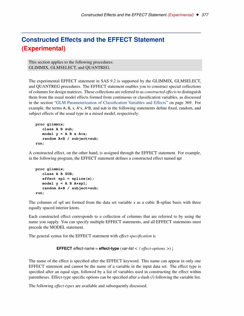
Constructed Effects and the EFFECT Statement(Experimental)

This section applies to the following procedures:GLIMMIX, GLMSELECT, and QUANTREG.

The experimental EFFECT statement in SAS 9.2 is supported by the GLIMMIX, GLMSELECT,and QUANTREG procedures. The EFFECT statement enables you to construct special collectionsof columns for design matrices. These collections are referred to as constructed effects to distinguishthem from the usual model effects formed from continuous or classification variables, as discussedin the section “GLM Parameterization of Classification Variables and Effects” on page 369. Forexample, the terms A, B, x, A*x, A*B, and sub in the following statements define fixed, random, andsubject effects of the usual type in a mixed model, respectively:

proc glimmix;class A B sub;model y = A B x A*x;random A*B / subject=sub;

run;

A constructed effect, on the other hand, is assigned through the EFFECT statement. For example,in the following program, the EFFECT statement defines a constructed effect named spl:

proc glimmix;class A B SUB;effect spl = spline(x);model y = A B A*spl;random A*B / subject=sub;

run;

The columns of spl are formed from the data set variable x as a cubic B-spline basis with threeequally spaced interior knots.

Each constructed effect corresponds to a collection of columns that are referred to by using thename you supply. You can specify multiple EFFECT statements, and all EFFECT statements mustprecede the MODEL statement.

The general syntax for the EFFECT statement with effect-specification is

EFFECT effect-name = effect-type (var-list < / effect-options >) ;

The name of the effect is specified after the EFFECT keyword. This name can appear in only oneEFFECT statement and cannot be the name of a variable in the input data set. The effect type isspecified after an equal sign, followed by a list of variables used in constructing the effect withinparentheses. Effect-type specific options can be specified after a slash (/) following the variable list.

The following effect-types are available and subsequently discussed.


COLLECTION is a collection effect defining one or more variables as a single effectwith multiple degrees of freedom. The variables in a collection areconsidered as a unit for estimation and inference.

MULTIMEMBER | MM is a multimember classification effect whose levels are determinedby one or more variables that appear in a CLASS statement.

POLYNOMIAL | POLY is a multivariate polynomial effect in the specified numeric vari-ables.

SPLINE is a regression spline effect whose columns are univariate spline ex-pansions of one or more variables. A spline expansion replaces theoriginal variable with an expanded or larger set of new variables.

Collection Effects

EFFECT name=COLLECTION(var-list < / DETAILS >) ;

You use a collection effect to define a set of variables that are treated as a single effect with mul-tiple degrees of freedom. The variables in var-list can be continuous or classification variables.The columns in the design matrix contributed by a collection effect are the design columns of itsconstituent variables in the order in which they appear in the definition of the collection effect. Ifyou specify the DETAILS option, then a table showing the constituents of the collection effect isdisplayed.

Multimember Effects

EFFECT name=MULTIMEMBER(var-list < / mm-options >) ;

EFFECT name=MM(var-list < / mm-options >) ;

A multimember effect is formed from one or more classification variables in such a way that eachobservation can be associated with one or more levels of the union of the levels of the classificationvariables. In other words, a multimember effect is a classification-type effect with possibly morethan one nonzero column entry for each observation. Multimember effects are useful, for example,in modeling the following:

� nurses’ effects on patient recovery in hospitals

� teachers’ effects on student scores

� lineage effects in genetic studies (see Example 38.16 in Chapter 38, “The GLIMMIX Proce-dure,” for an application with random multimember effects in a genetic diallel experiment)

The levels of a multimember effect consist of the union of formatted values of the variables definingthis effect. Each such level contributes one column to the design matrix. For each observation, the

Multimember Effects F 379

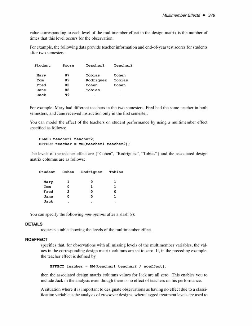
value corresponding to each level of the multimember effect in the design matrix is the number oftimes that this level occurs for the observation.

For example, the following data provide teacher information and end-of-year test scores for studentsafter two semesters:

Student Score Teacher1 Teacher2

Mary 87 Tobias CohenTom 89 Rodriguez TobiasFred 82 Cohen CohenJane 88 Tobias .Jack 99 . .

For example, Mary had different teachers in the two semesters, Fred had the same teacher in bothsemesters, and Jane received instruction only in the first semester.

You can model the effect of the teachers on student performance by using a multimember effectspecified as follows:

CLASS teacher1 teacher2;EFFECT teacher = MM(teacher1 teacher2);

The levels of the teacher effect are {“Cohen”, “Rodriguez”, “Tobias”} and the associated designmatrix columns are as follows:

Student Cohen Rodriguez Tobias

Mary 1 0 1Tom 0 1 1Fred 2 0 0Jane 0 0 1Jack . . .

You can specify the following mm-options after a slash (/):

DETAILSrequests a table showing the levels of the multimember effect.

NOEFFECTspecifies that, for observations with all missing levels of the multimember variables, the val-ues in the corresponding design matrix columns are set to zero. If, in the preceding example,the teacher effect is defined by

EFFECT teacher = MM(teacher1 teacher2 / noeffect);

then the associated design matrix columns values for Jack are all zero. This enables you toinclude Jack in the analysis even though there is no effect of teachers on his performance.

A situation where it is important to designate observations as having no effect due to a classi-fication variable is the analysis of crossover designs, where lagged treatment levels are used to


model the carryover effects of treatments between periods. Since there is no carryover effectfor the first period, the treatment lag effect in a crossover design can be modeled with a mul-timember effect that consists of a single classification variable and the NOEFFECT option,as in the following statements:

CLASS Treatment lagTreatment;EFFECT Carryover = MM(lagTreatment / noeffect);

The lagTreatment variable contains a missing value for the first period. Otherwise, it containsthe value of the treatment variable for the preceding period.

STDIZEspecifies that for each observation, the entries in the design matrix corresponding to the mul-timember effect are scaled to have a sum of one.

WEIGHT=(wght-list)specifies numeric variables used to weigh the contributions of each of the classification effectsthat define the constructed multimember effect. The number of variables in the WEIGHT=list must match the number of classification variables defining the effect.

Polynomial Effects

This section discusses the construction of multivariate polynomial effects through the experimentalEFFECT statement in the GLIMMIX and GLMSELECT procedures. You request a polynomialeffect with the syntax

EFFECT name=POLYNOMIAL(var-list < / polynomial-options >) ;

EFFECT name=POLY(var-list < / polynomial-options >) ;

The variables in var-list must be numeric. A design matrix column is generated for each term of thespecified polynomial. By default, each of these terms is treated as a separate effect for the purposeof model building. For example, the statements

proc glmselect;effect MyPoly = polynomial(x1-x3/degree=2);model y = MyPoly;

run;

yield the identical analysis to the statements

proc glmselect;model y = x1 x2 x3 x1*x1 x1*x2 x1*x3 x2*x2 x2*x3 x3*x3;

run;

You can specify the following polynomial-options after a slash (/):

DEGREE=nspecifies the degree of the polynomial. The degree must be a positive integer. The degree istypically a small integer, such as 1, 2, or 3. The default is DEGREE=1.

Polynomial Effects F 381

DETAILSrequests a table showing the details of the specified polynomial, including the number ofterms generated. If you specify the STANDARDIZE option, then a table showing the stan-dardization details is also produced.

LABELSTYLE=(style-opts)

LABELSTYLE=style-optspecifies how the terms in the polynomial are labeled. By default, powers are shown with ˆ asthe exponentiation operator and � as the multiplication operator. For example, a polynomialterm such as x3

1x2x23 is labeled x1ˆ3*x2*x3ˆ2. You can change the style of the label by using

the following style-opts within parentheses. If you specify a single style-opt, then you canomit the enclosing parentheses.

EXPANDspecifies that each variable with an exponent greater than one is written as products ofthat variable. For example, the term x3

1x2x23 receives the label x1*x1*x1*x2*x3*x3.

EXPONENT < =quoted string >specifies that each variable with an exponent greater than one is written using expo-nential notation. By default, the symbol ˆ is used as the exponentiation operator. Ifyou supply the optional quoted string after an equal sign, then that string is used as theexponentiation operator. For example, if you specify

LABELSTYLE=(EXPONENT="**")

then the term x31x2x

23 receives the label x1**3*x2*x3**2.

INCLUDENAMEspecifies that the name of the effect followed by an underscore is used as a prefix forterm labels. For example, the statement

EFFECT MyPoly=POLYNOMIAL(x1/degree=2 labelstyle=INCLUDENAME)

generates terms with labels MyPoly_x1 and MyPoly_x1ˆ2. The INCLUDENAME optionis ignored if you specify the NOSEPARATE option in the EFFECT=POLYNOMIALstatement.

PRODUCTSYMBOL =NONE | quoted stringspecifies that the supplied string be used as the product symbol. For example, thestatement

EFFECT MyPoly=POLYNOMIAL(x1 x2 / degree=2 mdegree=1labelstyle=(PRODUCTSYMBOL=" "))

generates terms with labels x1, x2, and x1 x2.

If you specify PRODUCTSYMBOL=NONE, then the labels are formed by juxtaposingthe constituent variable names.

MDEGREE=nspecifies the maximum degree of any variable in a term of the polynomial. This degree must


be a positive integer. The default is the degree of the specified polynomial. For example, thestatement

EFFECT MyPoly=POLYNOMIAL(x1 x2/degree=4 MDEGREE=2);

generates the terms x1, x2, x21 , x1x2, x2

2 ,x21x2, and x1x

22 .

NOSEPARATEspecifies that the polynomial is treated as a single effect with multiple degrees of freedom.The effect name that you specify is used as the constructed effect name and the labels of theterms are used as labels of the corresponding parameters.

STANDARDIZE < (centerscale-opts) > < = standardize-opt >specifies that the variables defining the polynomial are standardized. By default, the stan-dardized variables receive prefix “s_” in the variable names.

You can use the following centerscale-opts to specify how the center and scale are estimated:

METHOD=MOMENTSspecifies that the center is estimated by the variable mean and the scale is estimatedby the standard deviation. Note that if a weight variable is specified using a WEIGHTstatement, the observations with invalid weights are ignored when forming the meanand standard deviation, but the weights are otherwise not used. Note that only observa-tions that are used in performing the analysis are used for the standardization.

METHOD=RANGEspecifies that the center is estimated by the midpoint of the variable range and the scaleis estimated as half the variable range. Any observation that has a missing value for anyregressor used in the model is ignored when computing the range of variables in a poly-nomial effect. Observations with valid regressor values but missing or invalid valuesof frequency variables, weight variables, or dependent variables are used in comput-ing variable ranges. The default (if you do not specify the METHOD= suboption) isMETHOD=RANGE.

METHOD=WMOMENTSis the same as METHOD=MOMENTS except that weighted means and weighted stan-dard deviations are used.

Polynomial Effects F 383

Let

n D number of observations used in the analysis

w D weight variable

f D frequency variable

x D variable to be standardized

x.n/ D MaxniD1.xi /

x.1/ D MinniD1.xi /

F D sum of frequencies

D †niD1fi

WF D sum of weighted frequencies

D †niD1wifi

Table 18.9 shows how the center and scale are computed for each of the supported methods:

Table 18.9 Center and Scale Estimates by Method

Method Center Scale

Range .x.n/ � x.1//=2 .x.n/ C x.1//=2

Moments Nx D †niD1fixi=F

q†n

iD1fi .xi � Nx/2=.F � 1/

WMoments Nxw D †niD1wifixi=WF

q†n

iD1wifi .xi � Nxw/2=.F � 1/

PREFIX=NONE | quoted stringspecifies the prefix that is appended to standardized variables when forming the term la-bels. If you omit this option, the default prefix is “s_”. If you specify PREFIX=NONE,then standardized variables are not prefixed.

You can control whether the standardization is to center, scale, or both center and scale byspecifying a standardize-opt:

CENTERspecifies that variables are centered but not scaled. For a variable x,

s_x D x � center

CENTERSCALEspecifies that variables are centered and scaled. This is the default if you do not specifya standardization-opt. For a variable x,

s_x Dx � center

scale

NONEspecifies that no standardization is performed.


SCALEspecifies that variables are scaled but not centered. For a variable x,

s_x Dx

scale

Spline Effects

This section discusses the construction of spline effects through the experimental EFFECT state-ment in the GLIMMIX, GLMSELECT, and QUANTREG procedures. You can also include splineeffects in statistical models by other means. The TRANSREG procedure has dedicated facilitiesfor including regression splines in your model and controlling the construction of the splines. Forexample, you can use the TRANSREG procedure to fit a spline function but restrict the functionto be always increasing or decreasing (monotone). See the section “Using Splines and Knots” onpage 7184 in Chapter 90, “The TRANSREG Procedure,” for more information about using splineswith the TRANSREG procedure. The GAM and TPSPLINE procedures also can model the effectsof regressor variables in terms of smooth functions that are generated from spline bases. For moreinformation see Chapter 36, “The GAM Procedure,” and Chapter 89, “The TPSPLINE Procedure.”

A spline effect expands variables into spline bases whose form depends on the options that youspecify. You can find details about regression splines and spline bases in the section “Splines andSpline Bases” on page 387. You request a spline effect with the syntax

EFFECT name=SPLINE(var-list < / spline-options >) ;

The variables in var-list must be numeric. Design matrix columns are generated separately for eachof these variables and the set of columns is collectively referred to with the specified name. Bydefault, the spline basis generated for each variable is a cubic B-spline basis with three equallyspaced knots positioned between the minimum and maximum values of that variable. This yieldsby default seven design matrix columns for each of the variables in the SPLINE effect.

You can specify the following spline-options after a slash (/):

BASIS=BSPLINEspecifies a B-spline basis for the spline expansion. For splines of degree d defined withn knots, this basis consists of n C d C 1 columns. In order to completely specify the B-spline basis, d left-side boundary knots and maxfd; 1g right-side boundary knots are alsorequired. See the suboptions KNOTMETHOD=, DATABOUNDARY=, KNOTMIN=, andKNOTMAX= for details about how to specify the positions of both the internal and boundaryknots. This is the default if you do not specify the BASIS= suboption.

BASIS=TPF(options)specifies a truncated power function basis for the spline expansion. For splines of degreed defined with n knots for a variable x, this basis consists of an intercept, polynomials x,x2,: : : ,xd and one truncated power function for each of the n knots. Note that unlike the B-spline basis no boundary knots are required. See the suboption KNOTMETHOD= for detailsabout how you can specify the position of the internal knots.

You can modify the number of columns when you request BASIS=TPF with the followingsuboptions:

Spline Effects F 385

NOINTexcludes the intercept column.

NOPOWERSexcludes the intercept and polynomial columns.

DATABOUNDARYspecifies that the extremes of the data be used as boundary knots when building a B-splinebasis.

DEGREE=nspecifies the degree of the spline transformation. The degree must be a nonnegative integer.The degree is typically a small integer, such as 0, 1, 2, or 3. The default is DEGREE=3.

DETAILSrequests tables showing the knot locations and the knots associated with each spline basisfunction.

KNOTMAX=valuespecifies that, for each variable in the EFFECT statement, the right-side boundary knots beequally spaced starting at the maximum of the variable and ending at the specified value. Thisoption is ignored for variables whose maximum value is greater than the specified value or ifthe DATABOUNDARY option is also specified.

KNOTMETHOD=knot-method< (knot-options) >specifies how the knots for spline effects are constructed. You can choose from the followingknot-methods and affect the knot construction further with the type-specific knot-options:

EQUAL< (n) >specifies that n equally spaced knots be positioned between the extremes of the data.The default is n D 3. For a B-spline basis, any needed boundary knots continue to beequally spaced unless the DATABOUNDARY option has also been specified. KNOT-METHOD=EQUAL is the default if no knot-method is specified.

LIST(number-list)specifies the list of internal knots to be used in forming the spline basis columns. For aB-spline basis, the data extremes are used as boundary knots.

LISTWITHBOUNDARY(number-list)specifies the list of all knots in forming the spline basis columns. When you use a trun-cated power function basis, this list is interpreted as the list of internal knots. When youuse a B-spline basis of degree d , then the first d entries are used as left-side boundaryknots and the last MAX.d; 1/ entries in the list are used as right-side boundary knots.

MULTISCALE< (multiscale-options) >specifies that multiple B-spline bases be generated, corresponding to sets with an in-creasing number of internal knots. As you increase the number of internal knots, thespline basis you generate is able to approximate features of the data at finer scales. So,by generating bases at multiple scales, you facilitate the modeling of both coarse- andfine-grained features of the data. For scale i , the spline basis corresponds to 2i equally


spaced internal knots. By default, the bases for scales 0–7 are generated. For each scale,a separate spline effect is generated. The name of the constructed spline effect at scalei is formed by appending _Si to the effect name you specify in the EFFECT statement.If you specify multiple variables in the EFFECT statement, then spline bases are gener-ated separately for each variable at each scale and the name of the corresponding effectis obtained by appending the variable name followed by _Si to the name in the EFFECTstatement. For example, the following statement generates effects named spl_x1_S0,spl_x1_S1, spl_x1_S2, : : :, spl_x1_S7 and spl_x2_S1, spl_x2_S2, : : :, spl_x2_S7:

EFFECT spl = spline(x1 x2 / knotmethod=multiscale);

This option is ignored if you specify the BASIS=TPF suboption. It is not available forspline effects specified in the RANDOM statement of the GLIMMIX procedure.

You can control which scales are included with the following multiscale-options:

STARTSCALE=nwhere n is a positive integer. The default is STARTSCALE=0.

ENDSCALE=nwhere n is a positive integer. The default is ENDSCALE=7.

PERCENTILES(n)requests that internal knots be placed at n equally spaced percentiles of the variable orvariables named in the EFFECT statement. For example, the following statement posi-tions internal knots at the deciles of the variable x. For a B-spline basis, the extremesof the data are used as boundary knots:

EFFECT spl = spline(x / knotmethod=percentiles(9));

RANGEFRACTIONS(fraction-list)requests that internal knots be placed at each fraction of the ranges of the variables in theEFFECT statement. For example, if variable x1 ranges between 1 and 3, and variablex2 ranges between 0 and 20, then the following EFFECT statement uses internal knots1.2, 2, and 2.5 for variable x1 and internal knots 2, 10, and 15 for variable x2:

EFFECT spl = spline(x1 x2 / knotmethod=rangefractions(.1 .5 .75));

For a B-spline basis, the data extremes are used as boundary knots.

KNOTMIN=valuespecifies that for each variable in the EFFECT statement, the left-side boundary knots beequally spaced starting at the specified value and ending at the minimum of the variable. Thisoption is ignored for variables whose minimum value is less than the specified value or if theDATABOUNDARY option is also specified.

SEPARATEspecifies that when multiple variables are specified in the EFFECT statement, the spline basisfor each variable is treated as a separate effect. The names of these separated effects areformed by appending an underscore followed by the name of the variable to the name thatyou specify in the EFFECT statement. For example, the effect names generated with thefollowing statement are spl_x1 and spl_x2:

Splines and Spline Bases F 387

EFFECT spl = spline(x1 x2 / separate);

In procedures that support variable selection, such as the GLMSELECT procedure, these twoeffects can enter or leave the model independently during the selection process. Separatedeffects are not supported in the RANDOM statement of the GLIMMIX procedure

SPLITspecifies that each individual column in the design matrix corresponding to the spline effect istreated as a separate effect that can enter or leave the model independently. Names for thesesplit effects are generated by appending the variable name and an index for each column tothe name that you specify in the EFFECT statement. For example, the effects generated forthe spline effect in the following statement are spl_x1:1, spl_x1:2, . . . ,spl_x1:7, spl_x2:1,spl_x2:2, . . . ,spl_x2:7:

EFFECT spl = spline(x1 x2 / split);

The SPLIT option is not supported in the GLIMMIX procedure.

Splines and Spline Bases

This section provides details about the construction of spline bases with the experimental EFFECTstatement. A spline function is a piecewise polynomial function where the individual polynomialshave the same degree and connect smoothly at join points whose abscissa values, referred to asknots, are prespecified. You can use spline functions to fit curves to a wide variety of data.

A spline of degree 0 is a step function with steps located at the knots. A spline of degree 1 is apiecewise linear function where the lines connect at the knots. A spline of degree 2 is a piecewisequadratic curve whose values and slopes coincide at the knots. A spline of degree 3 is a piecewisecubic curve whose values, slopes, and curvature coincide at the knots. Visually, a cubic spline isa smooth curve, and it is the most commonly used spline when a smooth fit is desired. Note thatwhen no knots are used, splines of degree d are simply polynomials of degree d .

More formally, suppose you specify knots k1 < k2 < k3 < � � � < kn. Then a spline of degreed � 0 is a function S.x/ with d � 1 continuous derivatives such that

S.x/ D

8<:P0.x/ x < k1

Pi .x/ ki � x < kiC1I i D 1; 2; : : : ; n � 1

Pn.x/ x � kn

where each Pi .x/ is a polynomial of degree d . The requirement that S.x/ has d � 1 continuousderivatives is satisfied by requiring that the function values and all derivatives up to order d � 1 ofthe adjacent polynomials at each knot match.

A counting argument yields the number of parameters that define a spline with n knots. There arenC1 polynomials of degree d , giving .nC1/.dC1/ coefficients. However, there are d restrictionsat each of the n knots, so the number of free parameters is .nC 1/.d C 1/ � nd = nC d C 1. Inmathematical terminology this says that the dimension of the vector space of splines of degree d onn distinct knots is nC d C 1. If you have nC d C 1 basis vectors, then you can fit a curve to your


data by regressing your dependent variable by using this basis for the corresponding design matrixcolumns. In this context, such a spline is known as a regression spline. The EFFECT statementprovides a simple mechanism for obtaining such a basis.

If you remove the restriction that the knots of a spline must be distinct and allow repeated knots,then you can obtain functions with less smoothness and even discontinuities at the repeated knotlocation. For a spline of degree d and a repeated knot with multiplicity m � d , the piecewisepolynomials that join such a knot are required to have only d �m matching derivatives. Note thatthis increases the number of free parameters by m � 1 but also decreases the number of distinctknots bym� 1. Hence the dimension of the vector space of splines of degree d with n knots is stillnC d C 1, provided that any repeated knot has a multiplicity less than or equal to d .

The EFFECT statement provides support for the commonly used truncated power function basisand B-spline basis. With exact arithmetic and by using the complete basis, you will obtain the samefit with either of these bases. The following sections provide details about constructing spline basesfor the space of splines of degree d with n knots satisfying k1 � k2 � k3 < � � � � kn.

Truncated Power Function Basis

A truncated power function for a knot ki is a function defined by

ti .x/ D

�0 x < ki

.x � ki /d x � ki

Figure 18.1 shows such functions for d D 1 and d D 3 with a knot at x D 1.

Figure 18.1 Truncated Power Functions with Knot at x D 1

The name is derived from the fact that these functions are shifted power functions that get truncatedto zero to the left of the knot. These functions are piecewise polynomial functions with two pieceswhose function values and derivatives of all orders up to d � 1 are zero at the defining knot. Hencethese functions are splines of degree d . It is easy to see that these n functions are linearly inde-pendent. However, they do not form a basis, because such a basis requires n C d C 1 functions.The usual way to add d C 1 additional basis functions is to use the polynomials 1; x; x2; : : : ; xd .

Splines and Spline Bases F 389

These d C1 functions together with the n truncated power functions ti .x/; i D 1; 2; : : : ; n form thetruncated power basis.

Note that each time a knot is repeated, the associated exponent used in the corresponding basisfunction is reduced by 1. For example, for splines of degree d with 3 repeated knots ki D kiC1 D

kiC2 the corresponding basis functions are ti .x/ D ..x � ki /dC

, tiC1.x/ D ..x � ki /d�1C

, andtiC2.x/ D ..x � ki /

d�2C

. Provided that the multiplicity of each repeated knot is less than or equalto the degree, this construction continues to yield a basis for the associated space of splines.

The main advantage of the truncated power function basis is the simplicity of its construction andthe ease of interpreting the parameters in a model corresponding to these basis functions. However,there are two weaknesses when you use this basis for regression. These functions grow rapidlywithout bound as x increases, resulting in numerical precision problems when the x data span awide range. Furthermore, many or even all of these basis functions can be nonzero when evaluatedat some x value, resulting in a design matrix with few zeros that precludes the use of sparse matrixtechnology to speed up computation. This weakness can be addressed by using a B-spline basis.

B-Spline Basis

A B-spline basis can be built by starting with a set of Haar basis functions, which are functionsthat are 1 between adjacent knots and zero elsewhere, and then applying a simple linear recursionrelationship d times, yielding the nCd C1 needed basis functions. For the purpose of building theB-spline basis, the n prespecified knots are referred to as internal knots. This construction requiresd additional knots, known as boundary knots, to be positioned to the left of the internal knots, andMAX.d; 1/ boundary knots to be positioned to the right of the internal knots. The actual valuesof these boundary knots can be arbitrary. The EFFECT statement provides several methods forplacing the needed boundary knots, including the common method of using repeated values of thedata extremes as the boundary knots. The boundary knot placement affects the precise form of thebasis functions generated but not the following two desirable properties:

1. The B-spline basis functions are nonzero over an interval spanning at most d C 2 knots. Thisyields design matrix columns each of whose rows contain at most d C 2 adjacent nonzeroentries.

2. The computation of the basis functions at any x value is numerically stable and does notrequire evaluating powers of this value.

The following figures show the B-spline bases defined on Œ0; 1� with 4 equally spaced internal knotsat 0.2, 0.4, 0.6, and 0.8.

Figure 18.2 shows a linear B-spline basis. Note that this basis consists of 6 functions each of whichis nonzero over an interval spanning at most 3 knots.


Figure 18.2 Linear B-Spline Basis with Four Equally Spaced Interior Knots

Figure 18.3 shows a cubic B-spline basis where the needed boundary knots are positioned at x D 0

and x D 1. Note that this basis consists of 8 functions, each of which is nonzero over an intervalspanning at most 5 knots.

Figure 18.3 Cubic B-Spline Basis with Four Equally Spaced Interior Knots

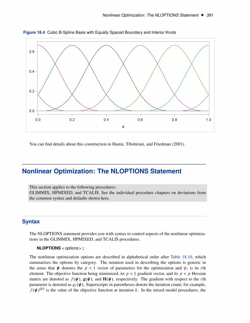
Figure 18.4 shows a different cubic B-spline basis where the needed left-side boundary knots arepositioned at �0:6, �0:4, �0:2, and 0. The right-side boundary knots are positioned at 1, 1:2, 1:4,and 1:6. Note that, as in the basis shown in Figure 18.3, this basis consists of 8 functions, eachof which is nonzero over an interval spanning at most 5 knots. The different positioning of theboundary knots has merely changed the shape of the individual basis functions.

Nonlinear Optimization: The NLOPTIONS Statement F 391

Figure 18.4 Cubic B-Spline Basis with Equally Spaced Boundary and Interior Knots

You can find details about this construction in Hastie, Tibshirani, and Friedman (2001).

Nonlinear Optimization: The NLOPTIONS Statement

This section applies to the following procedures:GLIMMIX, HPMIXED, and TCALIS. See the individual procedure chapters on deviations fromthe common syntax and defaults shown here.

Syntax

The NLOPTIONS statement provides you with syntax to control aspects of the nonlinear optimiza-tions in the GLIMMIX, HPMIXED, and TCALIS procedures.

NLOPTIONS < options > ;

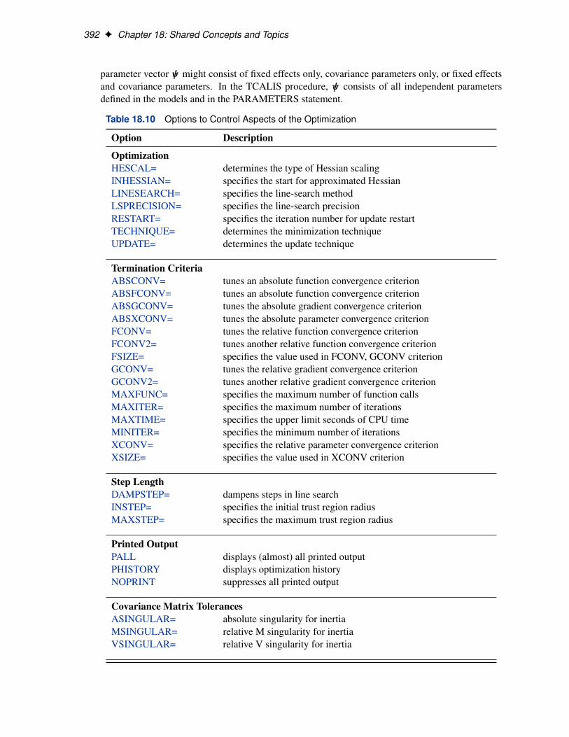
The nonlinear optimization options are described in alphabetical order after Table 18.10, whichsummarizes the options by category. The notation used in describing the options is generic inthe sense that denotes the p � 1 vector of parameters for the optimization and i is its i thelement. The objective function being minimized, its p � 1 gradient vector, and its p � p Hessianmatrix are denoted as f . /, g. /, and H. /, respectively. The gradient with respect to the i thparameter is denoted as gi . /. Superscripts in parentheses denote the iteration count; for example,f . /.k/ is the value of the objective function at iteration k. In the mixed model procedures, the


parameter vector might consist of fixed effects only, covariance parameters only, or fixed effectsand covariance parameters. In the TCALIS procedure, consists of all independent parametersdefined in the models and in the PARAMETERS statement.

Table 18.10 Options to Control Aspects of the Optimization

Option Description

OptimizationHESCAL= determines the type of Hessian scalingINHESSIAN= specifies the start for approximated HessianLINESEARCH= specifies the line-search methodLSPRECISION= specifies the line-search precisionRESTART= specifies the iteration number for update restartTECHNIQUE= determines the minimization techniqueUPDATE= determines the update technique

Termination CriteriaABSCONV= tunes an absolute function convergence criterionABSFCONV= tunes an absolute function convergence criterionABSGCONV= tunes the absolute gradient convergence criterionABSXCONV= tunes the absolute parameter convergence criterionFCONV= tunes the relative function convergence criterionFCONV2= tunes another relative function convergence criterionFSIZE= specifies the value used in FCONV, GCONV criterionGCONV= tunes the relative gradient convergence criterionGCONV2= tunes another relative gradient convergence criterionMAXFUNC= specifies the maximum number of function callsMAXITER= specifies the maximum number of iterationsMAXTIME= specifies the upper limit seconds of CPU timeMINITER= specifies the minimum number of iterationsXCONV= specifies the relative parameter convergence criterionXSIZE= specifies the value used in XCONV criterion

Step LengthDAMPSTEP= dampens steps in line searchINSTEP= specifies the initial trust region radiusMAXSTEP= specifies the maximum trust region radius

Printed OutputPALL displays (almost) all printed outputPHISTORY displays optimization historyNOPRINT suppresses all printed output

Covariance Matrix TolerancesASINGULAR= absolute singularity for inertiaMSINGULAR= relative M singularity for inertiaVSINGULAR= relative V singularity for inertia

Syntax F 393

Table 18.10 continued

Option Description

Constraint SpecificationsLCEPSILON= range for active constraintsLCDEACT= LM tolerance for deactivatingLCSINGULAR= tolerance for dependent constraints

Remote MonitoringSOCKET= specifies the fileref for remote monitoring

ABSCONV=r

ABSTOL=rspecifies an absolute function convergence criterion. For minimization, termination requiresf . .k// � r . The default value of r is the negative square root of the largest double-precisionvalue, which serves only as a protection against overflows.

ABSFCONV=r < n >

ABSFTOL=r< n >specifies an absolute function convergence criterion. For all techniques except NMSIMP,termination requires a small change of the function value in successive iterations:

jf . .k�1// � f . .k//j � r

The same formula is used for the NMSIMP technique, but .k/ is defined as the vertex withthe lowest function value, and .k�1/ is defined as the vertex with the highest function valuein the simplex. The default value is r D 0. The optional integer value n specifies the numberof successive iterations for which the criterion must be satisfied before the process can beterminated.

ABSGCONV=r < n >

ABSGTOL=r< n >specifies an absolute gradient convergence criterion. Termination requires the maximum ab-solute gradient element to be small:

maxj

jgj . .k//j � r

This criterion is not used by the NMSIMP technique. The default value is r D1E�5. Theoptional integer value n specifies the number of successive iterations for which the criterionmust be satisfied before the process can be terminated.

ABSXCONV=r < n >

ABSXTOL=r< n >specifies an absolute parameter convergence criterion. For all techniques except NMSIMP,termination requires a small Euclidean distance between successive parameter vectors,

k .k/� .k�1/

k2� r


For the NMSIMP technique, termination requires either a small length ˛.k/ of the vertices ofa restart simplex,

˛.k/� r

or a small simplex size,

ı.k/� r

where the simplex size ı.k/ is defined as the L1 distance from the simplex vertex �.k/ withthe smallest function value to the other p simplex points .k/

l¤ �.k/:

ı.k/D

X l ¤y

k .k/

l� �.k/

k1

The default is r D1E�8 for the NMSIMP technique and r D 0 otherwise. The optionalinteger value n specifies the number of successive iterations for which the criterion must besatisfied before the process can terminate.

ASINGULAR=r

ASING=rspecifies an absolute singularity criterion for the computation of the inertia (number of posi-tive, negative, and zero eigenvalues) of the Hessian and its projected forms. The default valueis the square root of the smallest positive double-precision value.

DAMPSTEP< =r >specifies that the initial step length value ˛.0/ for each line search (used by the QUANEW,CONGRA, or NEWRAP technique) cannot be larger than r times the step length value usedin the former iteration. If the DAMPSTEP option is specified but r is not specified, the defaultis r D 2. The DAMPSTEP=r option can prevent the line-search algorithm from repeatedlystepping into regions where some objective functions are difficult to compute or where theycould lead to floating-point overflows during the computation of objective functions and theirderivatives. The DAMPSTEP=r option can save time-consuming function calls during theline searches of objective functions that result in very small steps.

FCONV=r< n >FTOL=r< n >

specifies a relative function convergence criterion. For all techniques except NMSIMP, ter-mination requires a small relative change of the function value in successive iterations,

jf . .k// � f . .k�1//j

max.jf . .k�1//j;FSIZE/� r

where FSIZE is defined by the FSIZE= option. The same formula is used for the NMSIMPtechnique, but .k/ is defined as the vertex with the lowest function value, and .k�1/ isdefined as the vertex with the highest function value in the simplex.

The default is r D 10�FDIGITS, where FDIGITS is by default � log10f�g and � is the ma-chine precision. Some procedures, such as the GLIMMIX procedure, enable you to changethe value with the FDIGITS= option in the PROC statement. The optional integer value nspecifies the number of successive iterations for which the criterion must be satisfied beforethe process can terminate.

Syntax F 395

FCONV2=r< n >

FTOL2=r< n >specifies a second function convergence criterion. For all techniques except NMSIMP, termi-nation requires a small predicted reduction,

df .k/� f . .k// � f . .k/

C s.k//

of the objective function. The predicted reduction

df .k/D �g.k/0

s.k/�1

2s.k/0

H.k/s.k/

D �1

2s.k/0

g.k/� r

is computed by approximating the objective function f by the first two terms of the Taylorseries and substituting the Newton step,

s.k/D �ŒH.k/��1g.k/

For the NMSIMP technique, termination requires a small standard deviation of the functionvalues of the p C 1 simplex vertices .k/

l, l D 0; : : : ; p,s

1

nC 1

Xl

hf .

.k/

l/ � f . .k//

i2� r

where f . .k// D1

pC1

Pl f .

.k/

l/. If there are pact boundary constraints active at .k/,

the mean and standard deviation are computed only for the nC1�pact unconstrained vertices.The default value is r D1E�6 for the NMSIMP technique and r D 0 otherwise. The optionalinteger value n specifies the number of successive iterations for which the criterion must besatisfied before the process can terminate.

FSIZE=rspecifies the FSIZE parameter of the relative function and relative gradient termination crite-ria. The default value is r D 0. For more details, see the FCONV= and GCONV= options.

GCONV=r< n >

GTOL=r< n >specifies a relative gradient convergence criterion. For all techniques except CONGRA andNMSIMP, termination requires that the normalized predicted function reduction be small,

g. .k//0ŒH.k/��1g. .k//

max.jf . .k//j;FSIZE/� r

where FSIZE is defined by the FSIZE= option. For the CONGRA technique (where a reliableHessian estimate H is not available), the following criterion is used:

k g. .k// k22 k s. .k// k2

k g. .k// � g. .k�1// k2 max.jf . .k//j;FSIZE/� r

This criterion is not used by the NMSIMP technique. The default value is r D1E�8. Theoptional integer value n specifies the number of successive iterations for which the criterionmust be satisfied before the process can terminate.


GCONV2=r< n >

GTOL2=r< n >specifies another relative gradient convergence criterion. For least-squares problems andthe TRUREG, LEVMAR, NRRIDG, and NEWRAP techniques, the following criterion ofBrowne (1982) is used:

maxj

jgj . .k//jq

f . .k//H.k/j;j

� r

This criterion is not used by the other techniques. The default value is r D 0. The optionalinteger value n specifies the number of successive iterations for which the criterion must besatisfied before the process can terminate.

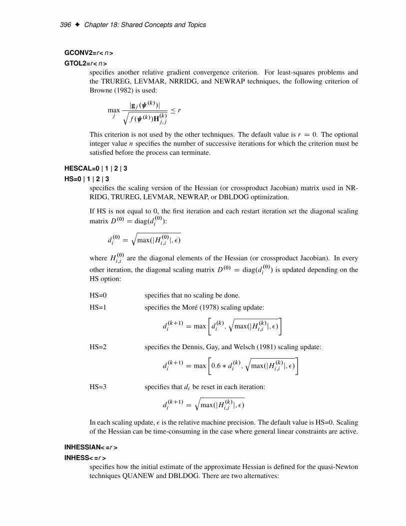
HESCAL=0 | 1 | 2 | 3

HS=0 | 1 | 2 | 3specifies the scaling version of the Hessian (or crossproduct Jacobian) matrix used in NR-RIDG, TRUREG, LEVMAR, NEWRAP, or DBLDOG optimization.

If HS is not equal to 0, the first iteration and each restart iteration set the diagonal scalingmatrix D.0/ D diag.d .0/

i /:

d.0/i D

qmax.jH .0/

i;i j; �/

where H .0/i;i are the diagonal elements of the Hessian (or crossproduct Jacobian). In every

other iteration, the diagonal scaling matrix D.0/ D diag.d .0/i / is updated depending on the

HS option:

HS=0 specifies that no scaling be done.

HS=1 specifies the Moré (1978) scaling update:

d.kC1/i D max

�d

.k/i ;

qmax.jH .k/

i;i j; �/

�HS=2 specifies the Dennis, Gay, and Welsch (1981) scaling update:

d.kC1/i D max

�0:6 � d

.k/i ;

qmax.jH .k/

i;i j; �/

�HS=3 specifies that di be reset in each iteration:

d.kC1/i D

qmax.jH .k/

i;i j; �/

In each scaling update, � is the relative machine precision. The default value is HS=0. Scalingof the Hessian can be time-consuming in the case where general linear constraints are active.

INHESSIAN< =r >

INHESS< =r >specifies how the initial estimate of the approximate Hessian is defined for the quasi-Newtontechniques QUANEW and DBLDOG. There are two alternatives:

Syntax F 397

� If you do not use the r specification, the initial estimate of the approximate Hessian isset to the Hessian at .0/.

� If you do use the r specification, the initial estimate of the approximate Hessian is setto the multiple of the identity matrix rI.

By default, if you do not specify the option INHESSIAN=r , the initial estimate of the approx-imate Hessian is set to the multiple of the identity matrix rI, where the scalar r is computedfrom the magnitude of the initial gradient.

INSTEP=r

SALPHA=r

RADIUS=rreduces the length of the first trial step during the line search of the first iterations. Forhighly nonlinear objective functions, such as the EXP function, the default initial radius ofthe trust-region algorithm TRUREG or DBLDOG or the default step length of the line-searchalgorithms can result in arithmetic overflows. If this occurs, you should specify decreasingvalues of 0 < r < 1 such as INSTEP=1E�1, INSTEP=1E�2, INSTEP=1E�4, and so on,until the iteration starts successfully.

� For trust-region algorithms (TRUREG, DBLDOG), the INSTEP= option specifies a fac-tor r > 0 for the initial radius �.0/ of the trust region. The default initial trust-regionradius is the length of the scaled gradient. This step corresponds to the default radiusfactor of r D 1.

� For line-search algorithms (NEWRAP, CONGRA, QUANEW), the INSTEP= optionspecifies an upper bound for the initial step length for the line search during the first fiveiterations. The default initial step length is r D 1.

� For the Nelder-Mead simplex algorithm, by using TECH=NMSIMP, the INSTEP=roption defines the size of the start simplex.

LCDEACT=r

LCD=rspecifies a threshold r for the Lagrange multiplier that determines whether an active inequal-ity constraint remains active or can be deactivated. For maximization, r must be greater thanzero; for minimization, r must be smaller than zero. An active inequality constraint can bedeactivated only if its Lagrange multiplier is less than the threshold value. The default valueis

r D ˙ min.0:01;max.0:1 � ABSGCONV; 0:001 � gmax.k///

where “+” stands for maximization, “-” stands for minimization, ABSGCONV is the value ofthe absolute gradient criterion, and gmax.k/ is the maximum absolute element of the gradientor the projected gradient.


LCEPSILON=r � 0

LCEPS=r � 0

LCE=r � 0

specifies the range for active and violated boundary constraints. If the point .k/ satisfies thecondition

j

kXj D1

aij .k/j � bi j � r � .jbi j C 1/

the constraint i is recognized as an active constraint. Otherwise, the constraint i is eitheran inactive inequality or a violated inequality or equality constraint. The default value isr D1E�8. During the optimization process, the introduction of rounding errors can forcethe optimization to increase the value of r by a factor of 10; 100; : : :. If this happens, it isindicated by a message displayed in the log.

LCSINGULAR=r � 0

LCSING=r � 0

LCS=r �

specifies a criterion r , used in the update of the QR decomposition, that determines whetheran active constraint is linearly dependent on a set of other active constraints. The defaultvalue is r D1E�8. The larger r becomes, the more the active constraints are recognized asbeing linearly dependent. If the value of r is larger than 0:1, it is reset to 0:1.

LINESEARCH=i

LIS=ispecifies the line-search method for the CONGRA, QUANEW, and NEWRAP optimizationtechniques. See Fletcher (1987) for an introduction to line-search techniques. The value of ican be 1; : : : ; 8. For CONGRA, QUANEW, and NEWRAP, the default value is i D 2.

LIS=1 specifies a line-search method that needs the same number of function andgradient calls for cubic interpolation and cubic extrapolation; this methodis similar to one used by the Harwell subroutine library.

LIS=2 specifies a line-search method that needs more function than gradient callsfor quadratic and cubic interpolation and cubic extrapolation; this methodis implemented as shown in Fletcher (1987) and can be modified to anexact line search by using the LSPRECISION= option.

LIS=3 specifies a line-search method that needs the same number of function andgradient calls for cubic interpolation and cubic extrapolation; this methodis implemented as shown in Fletcher (1987) and can be modified to anexact line search by using the LSPRECISION= option.

LIS=4 specifies a line-search method that needs the same number of function andgradient calls for stepwise extrapolation and cubic interpolation.

LIS=5 specifies a line-search method that is a modified version of LIS=4.

LIS=6 specifies golden section line search (Polak 1971), which uses only functionvalues for linear approximation.

Syntax F 399

LIS=7 specifies bisection line search (Polak 1971), which uses only function val-ues for linear approximation.

LIS=8 specifies the Armijo line-search technique (Polak 1971), which uses onlyfunction values for linear approximation.

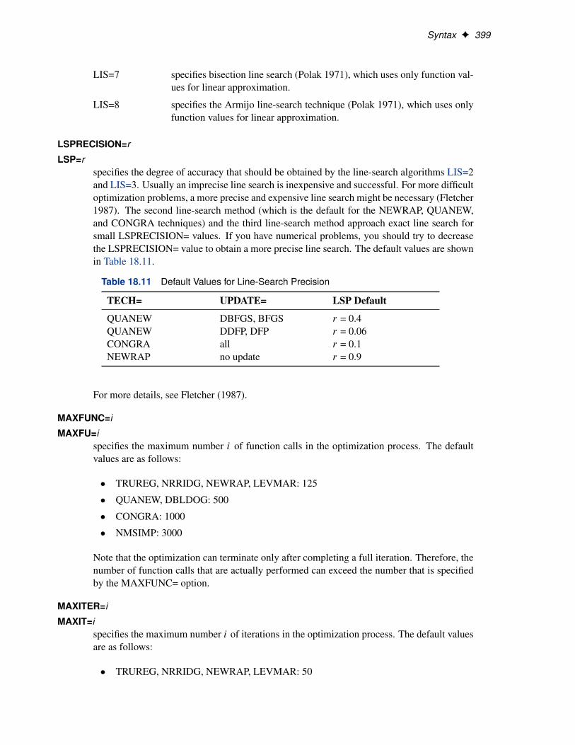
LSPRECISION=r

LSP=rspecifies the degree of accuracy that should be obtained by the line-search algorithms LIS=2and LIS=3. Usually an imprecise line search is inexpensive and successful. For more difficultoptimization problems, a more precise and expensive line search might be necessary (Fletcher1987). The second line-search method (which is the default for the NEWRAP, QUANEW,and CONGRA techniques) and the third line-search method approach exact line search forsmall LSPRECISION= values. If you have numerical problems, you should try to decreasethe LSPRECISION= value to obtain a more precise line search. The default values are shownin Table 18.11.

Table 18.11 Default Values for Line-Search Precision

TECH= UPDATE= LSP Default

QUANEW DBFGS, BFGS r = 0.4QUANEW DDFP, DFP r = 0.06CONGRA all r = 0.1NEWRAP no update r = 0.9

For more details, see Fletcher (1987).

MAXFUNC=i

MAXFU=ispecifies the maximum number i of function calls in the optimization process. The defaultvalues are as follows:

� TRUREG, NRRIDG, NEWRAP, LEVMAR: 125

� QUANEW, DBLDOG: 500

� CONGRA: 1000

� NMSIMP: 3000

Note that the optimization can terminate only after completing a full iteration. Therefore, thenumber of function calls that are actually performed can exceed the number that is specifiedby the MAXFUNC= option.

MAXITER=i

MAXIT=ispecifies the maximum number i of iterations in the optimization process. The default valuesare as follows:

� TRUREG, NRRIDG, NEWRAP, LEVMAR: 50


� QUANEW, DBLDOG: 200

� CONGRA: 400

� NMSIMP: 1000

These default values are also valid when i is specified as a missing value.

MAXSTEP=r< n >specifies an upper bound for the step length of the line-search algorithms during the first niterations. By default, r is the largest double-precision value and n is the largest integer avail-able. Setting this option can improve the speed of convergence for the CONGRA, QUANEW,and NEWRAP techniques.

MAXTIME=rspecifies an upper limit of r seconds of CPU time for the optimization process. The defaultvalue is the largest floating-point double representation of your computer. Note that the timespecified by the MAXTIME= option is checked only once at the end of each iteration. There-fore, the actual running time can be much longer than that specified by the MAXTIME=option. The actual running time includes the rest of the time needed to finish the iteration andthe time needed to generate the output of the results.

MINITER=i

MINIT=ispecifies the minimum number of iterations. The default value is 0. If you request moreiterations than are actually needed for convergence to a stationary point, the optimizationalgorithms can behave strangely. For example, the effect of rounding errors can prevent thealgorithm from continuing for the required number of iterations.

MSINGULAR=r > 0

MSING=r > 0specifies a relative singularity criterion for the computation of the inertia (number of positive,negative, and zero eigenvalues) of the Hessian and its projected forms. The default value is1E�12.

NOPRINTsuppresses output related to optimization such as the iteration history. The GLIMMIX andHPMIXED procedures do not support printing options in the NLOPTIONS statement.

PALLdisplays all optional output for optimization. This option is supported only by the TCALISprocedure.

PHISTORY

PHISTdisplays the optimization history. The PHISTORY option is implied if the PALL option isspecified. The PHISTORY option is supported only by the TCALIS procedure.

Syntax F 401

RESTART=i > 0

REST=i > 0specifies that the QUANEW or CONGRA algorithm is restarted with a steepest descent/ascentsearch direction after, at most, i iterations. Default values are as follows:

� CONGRA: UPDATE=PB: restart is performed automatically, i is not used.

� CONGRA: UPDATE¤PB: i D min.10p; 80/, where p is the number of parameters.

� QUANEW: i is the largest integer available.

SINGULAR=r

SING=rspecifies the singularity criterion r , r0 � r � 1, that is used for the inversion of the Hessianmatrix. The default value is 1E�8.

SOCKET=filerefspecifies the fileref that contains the information needed for remote monitoring. See thesection “Remote Monitoring” on page 403 for more details.

TECHNIQUE=value

TECH=value

OMETHOD=value

OM=valuespecifies the optimization technique. You can find additional information about choosing anoptimization technique in the section “Choosing an Optimization Algorithm” on page 405.Valid values for the TECHNIQUE= option are as follows:

� CONGRAperforms a conjugate-gradient optimization, which can be more precisely specified withthe UPDATE= option and modified with the LINESEARCH= option. When you specifythis option, UPDATE=PB by default.

� DBLDOGperforms a version of double-dogleg optimization, which can be more precisely speci-fied with the UPDATE= option. When you specify this option, UPDATE=DBFGS bydefault.

� LEVMARperforms a highly stable but, for large problems, memory- and time-consumingLevenberg-Marquardt optimization technique, a slightly improved variant of the Moré(1978) implementation. You can also specify this technique with the alias LM or MAR-QUARDT. In the TCALIS procedure, this is the default optimization technique if thereare fewer than 40 parameters to estimate. The GLIMMIX and HPMIXED proceduresdo not support this optimization technique.

� NMSIMPperforms a Nelder-Mead simplex optimization. The TCALIS procedure does not sup-port this optimization technique.

� NONEdoes not perform any optimization. This option can be used for the following:


– to perform a grid search without optimization– to compute estimates and predictions that cannot be obtained efficiently with any

of the optimization techniques– to obtain inferences for known values of the covariance parameters

� NEWRAPperforms a Newton-Raphson optimization combining a line-search algorithm with ridg-ing. The line-search algorithm LIS=2 is the default method.

� NRRIDGperforms a Newton-Raphson optimization with ridging.

� QUANEWperforms a quasi-Newton optimization, which can be defined more precisely with theUPDATE= option and modified with the LINESEARCH= option.

� TRUREGperforms a trust-region optimization.

UPDATE=method

UPD=methodspecifies the update method for the quasi-Newton, double-dogleg, or conjugate-gradient op-timization technique. Not every update method can be used with each optimizer.

The following are the valid methods for the UPDATE= option:

� BFGSperforms the original Broyden, Fletcher, Goldfarb, and Shanno (BFGS) update of theinverse Hessian matrix.

� DBFGSperforms the dual BFGS update of the Cholesky factor of the Hessian matrix. This isthe default update method.

� DDFPperforms the dual Davidon, Fletcher, and Powell (DFP) update of the Cholesky factorof the Hessian matrix.

� DFPperforms the original DFP update of the inverse Hessian matrix.

� PBperforms the automatic restart update method of Powell (1977) and Beale (1972).

� FRperforms the Fletcher-Reeves update (Fletcher 1987).

� PRperforms the Polak-Ribiere update (Fletcher 1987).

� CDperforms a conjugate-descent update of Fletcher (1987).

VERSION=1 | 2

VS=1 | 2specifies the version of the quasi-Newton optimization technique with nonlinear constraints.

Remote Monitoring F 403

VS=1 specifies the update of the � vector as in Powell (1978a, 1978b) (update like VF02AD).

VS=2 specifies the update of the � vector as in Powell (1982a, 1982b) (update like VMCWD).

The default is VERSION=2.

VSINGULAR=r > 0

VSING=r > 0specifies a relative singularity criterion for the computation of the inertia (number of positive,negative, and zero eigenvalues) of the Hessian and its projected forms. The default value isr D 1E�8.

XCONV=r< n >

XTOL=r< n >specifies the relative parameter convergence criterion. For all techniques except NMSIMP,termination requires a small relative parameter change in subsequent iterations:

maxj j .k/j �

.k�1/j j

max.j .k/j j; j

.k�1/j j;XSIZE/

� r

For the NMSIMP technique, the same formula is used, but .k/j is defined as the vertex with

the lowest function value and .k�1/j is defined as the vertex with the highest function value

in the simplex.

The default value is r D 1E�8 for the NMSIMP technique and r D 0 otherwise. The optionalinteger value n specifies the number of successive iterations for which the criterion must besatisfied before the process can be terminated.

XSIZE=rspecifies the XSIZE parameter of the relative parameter termination criterion, r � 0. Thedefault value is r D 0. For more details, see the XCONV= option.

Remote Monitoring

SAS/EmMonitor is an application for Windows that enables you to monitor a CPU-intensive ap-plication running on a remote server. Remote monitoring is support through the NLOPTIONSstatement.

On the server side, a FILENAME statement assigns a fileref to a SOCKET-type device that definesthe IP address of the client and the port number for listening. The fileref is then specified in theSOCKET= option in the NLOPTIONS statement to control the SAS/EmMonitor application. Thefollowing statements show an example of server-side code:


filename sock socket ’your.pc.address.com:6943’;

proc glimmix data=bigdataset;class year;model y1 = x1 x2 x3 / dist=gamma link=log;random x1 x3 / type=rsmooth knotmethod=kdtree(bucket=8)

subject=year;nloptions tech=nrridg gconv=2.e-5 socket=sock;

run;

On the client side, the SAS/EmMonitor application is started with the following syntax:

EmMonitor options

The options are as follows:

-p port_number defines the port number.

-t title defines the title of the SAS/EmMonitor window.

-k keeps the monitor alive when the iteration is completed.

The default port number is 6943.

By default, the PC client displays on its Graph tab the objective function of the optimization processas the first Plot Group. The largest absolute gradient can be monitored as the next Plot Group. Youcan intervene in the optimization process through the Stop Current and Stop All buttons. Signalingthe server by clicking these buttons effectively terminates the optimization. In a singly iterativeoptimization, clicking either of the two buttons halts the optimization process when the signal isreceived on the server side. The current parameter estimates are accepted, and postoptimizationprocessing is based on these values. Note that this is different from a condition where the usualtermination criterion is not met, such as when the maximum number of iterations is exceeded. If anoptimization does not meet the termination criterion, no postprocessing occurs.

In doubly iterative processes, the Stop All button terminates the overall optimization process andaccepts the current estimates. The Stop Current button stops the current optimization and uses thecurrent parameter estimates to start the next optimization.

The server does not need to be running when you start the SAS/EmMonitor application, and youcan start or stop it at any time during the iteration process. You need to remember only the portnumber.

If you do not start the PC client, or if you close it prematurely, it will have no effect on the serverside. In other words, the iteration process will continue until one of the criteria for termination ismet.

Choosing an Optimization Algorithm F 405

Choosing an Optimization Algorithm

First- or Second-Order Algorithms

The factors that go into choosing a particular optimization technique for a particular problem arecomplex. Trial and error can be involved.

For many optimization problems, computing the gradient takes more computer time than computingthe function value. Computing the Hessian sometimes takes much more computer time and memorythan computing the gradient, especially when there are many decision variables. Unfortunately,optimization techniques that do not use some kind of Hessian approximation usually require manymore iterations than techniques that do use a Hessian matrix, and, as a result, the total run time ofthese techniques is often longer. Techniques that do not use the Hessian also tend to be less reliable.For example, they can terminate more easily at stationary points than at global optima.

Table 18.12 shows which derivatives are required for each optimization technique (FOD: first-orderderivatives (=gradient evaluation); SOD: second-order derivatives (=Hessian evaluation)).

Table 18.12 First-Order and Second-Order Derivatives

Algorithm FOD SOD

LEVMAR x xTRUREG x xNEWRAP x xNRRIDG x xQUANEW x -DBLDOG x -CONGRA x -NMSIMP - -

The second-derivative methods TRUREG, NEWRAP, and NRRIDG are best for small problemswhere the Hessian matrix is not expensive to compute. Sometimes the NRRIDG algorithm canbe faster than the TRUREG algorithm, but TRUREG can be more stable. The NRRIDG algorithmrequires only one matrix with p.pC1/=2 double words; TRUREG and NEWRAP require two suchmatrices. Here, p denotes the number of parameters in the optimization.

The first-derivative methods QUANEW and DBLDOG are best for medium-sized problems wherethe objective function and the gradient are much faster to evaluate than the Hessian. The QUANEWand DBLDOG algorithms, in general, require more iterations than TRUREG, NRRIDG, andNEWRAP, but each iteration can be much faster. The QUANEW and DBLDOG algorithms re-quire only the gradient to update an approximate Hessian, and they require slightly less memorythan TRUREG or NEWRAP (essentially one matrix with p.p C 1/=2 double words).

The first-derivative method CONGRA is best for large problems where the objective function andthe gradient can be computed much faster than the Hessian and where too much memory is requiredto store the (approximate) Hessian. The CONGRA algorithm, in general, requires more iterationsthan QUANEW or DBLDOG, but each iteration can be much faster. Because CONGRA requires


only a factor of p double-word memory, many large applications can be solved only by CONGRA.

The no-derivative method NMSIMP is best for small problems where derivatives are not continuousor are very difficult to compute.

Each optimization method employs one or more convergence criteria that determine when it hasconverged. An algorithm is considered to have converged when any one of the convergence criteriais satisfied. For example, under the default settings, the QUANEW algorithm will converge ifABSGCONV <1E�5, FCONV < 10�FDIGITS , or GCONV <1E�8.

Algorithm Descriptions

Trust Region Optimization (TRUREG)

The trust region method uses the gradient g. .k// and the Hessian matrix H. .k//; thus, it re-quires that the objective function f . / have continuous first- and second-order derivatives insidethe feasible region.

The trust region method iteratively optimizes a quadratic approximation to the nonlinear objectivefunction within a hyperelliptic trust region with radius� that constrains the step size correspondingto the quality of the quadratic approximation. The trust region method is implemented based onDennis, Gay, and Welsch (1981), Gay (1983), and Moré and Sorensen (1983).

The trust region method performs well for small to medium-sized problems, and it does not needmany function, gradient, and Hessian calls. However, if the computation of the Hessian matrix iscomputationally expensive, one of the (dual) quasi-Newton or conjugate gradient algorithms mightbe more efficient.

Newton-Raphson Optimization with Line Search (NEWRAP)

The NEWRAP technique uses the gradient g. .k// and the Hessian matrix H. .k//; thus, it re-quires that the objective function have continuous first- and second-order derivatives inside thefeasible region. If second-order derivatives are computed efficiently and precisely, the NEWRAPmethod can perform well for medium-sized to large problems, and it does not need many function,gradient, and Hessian calls.

This algorithm uses a pure Newton step when the Hessian is positive definite and when the Newtonstep reduces the value of the objective function successfully. Otherwise, a combination of ridgingand line search is performed to compute successful steps. If the Hessian is not positive definite, amultiple of the identity matrix is added to the Hessian matrix to make it positive definite (Eskowand Schnabel 1991).

In each iteration, a line search is performed along the search direction to find an approximate op-timum of the objective function. The default line-search method uses quadratic interpolation andcubic extrapolation (LIS=2).


Newton-Raphson Ridge Optimization (NRRIDG)

The NRRIDG technique uses the gradient g. .k// and the Hessian matrix H. .k//; thus, it requiresthat the objective function have continuous first- and second-order derivatives inside the feasibleregion.

This algorithm uses a pure Newton step when the Hessian is positive definite and when the Newtonstep reduces the value of the objective function successfully. If at least one of these two conditionsis not satisfied, a multiple of the identity matrix is added to the Hessian matrix.

The NRRIDG method performs well for small to medium-sized problems, and it does not requiremany function, gradient, and Hessian calls. However, if the computation of the Hessian matrix iscomputationally expensive, one of the (dual) quasi-Newton or conjugate gradient algorithms mightbe more efficient.

Because the NRRIDG technique uses an orthogonal decomposition of the approximate Hessian,each iteration of NRRIDG can be slower than that of the NEWRAP technique, which works with aCholesky decomposition. Usually, however, NRRIDG requires fewer iterations than NEWRAP.

Quasi-Newton Optimization (QUANEW)

The (dual) quasi-Newton method uses the gradient g. .k//, and it does not need to compute second-order derivatives because they are approximated. It works well for medium-sized to moderatelylarge optimization problems, where the objective function and the gradient are much faster tocompute than the Hessian. However, in general, it requires more iterations than the TRUREG,NEWRAP, and NRRIDG techniques, which compute second-order derivatives. QUANEW is thedefault optimization algorithm because it provides an appropriate balance between the speed andstability required for most nonlinear mixed model applications.

The QUANEW technique is one of the following, depending upon the value of the UPDATE=option:

� the original quasi-Newton algorithm, which updates an approximation of the inverse Hessian

� the dual quasi-Newton algorithm, which updates the Cholesky factor of an approximate Hes-sian (default)

You can specify four update formulas with the UPDATE= option:

� DBFGS performs the dual Broyden, Fletcher, Goldfarb, and Shanno (BFGS) update of theCholesky factor of the Hessian matrix. This is the default.

� DDFP performs the dual Davidon, Fletcher, and Powell (DFP) update of the Cholesky factorof the Hessian matrix.

� BFGS performs the original BFGS update of the inverse Hessian matrix.

� DFP performs the original DFP update of the inverse Hessian matrix.


In each iteration, a line search is performed along the search direction to find an approximate opti-mum. The default line-search method uses quadratic interpolation and cubic extrapolation to obtaina step size ˛ satisfying the Goldstein conditions. One of the Goldstein conditions can be violated ifthe feasible region defines an upper limit of the step size. Violating the left-side Goldstein condi-tion can affect the positive definiteness of the quasi-Newton update. In that case, either the updateis skipped or the iterations are restarted with an identity matrix, resulting in the steepest descent orascent search direction. You can specify line-search algorithms other than the default with the LIS=option.

The QUANEW algorithm uses its own line-search technique. Not all options and parameters (exceptthe INSTEP= option) controlling the line search in the other algorithms apply here. In severalapplications, large steps in the first iterations are troublesome. You can use the INSTEP= optionto impose an upper bound for the step size ˛ during the first five iterations. You can also usethe INHESSIAN[=r] option to specify a different starting approximation for the Hessian. If youspecify only the INHESSIAN option, the Cholesky factor of a (possibly ridged) finite-differenceapproximation of the Hessian is used to initialize the quasi-Newton update process.

Double-Dogleg Optimization (DBLDOG)

The double-dogleg optimization method combines the ideas of the quasi-Newton and trust regionmethods. In each iteration, the double-dogleg algorithm computes the step s.k/ as the linear com-bination of the steepest descent or ascent search direction s.k/

1 and a quasi-Newton search directions.k/2 ,

s.k/D ˛1s.k/

1 C ˛2s.k/2

The step is requested to remain within a prespecified trust region radius; see Fletcher (1987, p.107). Thus, the DBLDOG subroutine uses the dual quasi-Newton update but does not perform aline search. You can specify two update formulas with the UPDATE= option:

� DBFGS performs the dual Broyden, Fletcher, Goldfarb, and Shanno update of the Choleskyfactor of the Hessian matrix. This is the default.

� DDFP performs the dual Davidon, Fletcher, and Powell update of the Cholesky factor of theHessian matrix.

The double-dogleg optimization technique works well for medium-sized to moderately large op-timization problems, where the objective function and the gradient are much faster to computethan the Hessian. The implementation is based on Dennis and Mei (1979) and Gay (1983), butit is extended for dealing with boundary and linear constraints. The DBLDOG technique gener-ally requires more iterations than the TRUREG, NEWRAP, or NRRIDG technique, which requiressecond-order derivatives; however, each of the DBLDOG iterations is computationally cheap. Fur-thermore, the DBLDOG technique requires only gradient calls for the update of the Cholesky factorof an approximate Hessian.

Conjugate Gradient Optimization (CONGRA)

Second-order derivatives are not required by the CONGRA algorithm and are not even approxi-mated. The CONGRA algorithm can be expensive in function and gradient calls, but it requires only


O.p/ memory for unconstrained optimization. In general, many iterations are required to obtaina precise solution, but each of the CONGRA iterations is computationally cheap. You can spec-ify four different update formulas for generating the conjugate directions by using the UPDATE=option:

� PB performs the automatic restart update method of Powell (1977) and Beale (1972). This isthe default.

� FR performs the Fletcher-Reeves update (Fletcher 1987).

� PR performs the Polak-Ribiere update (Fletcher 1987).

� CD performs a conjugate-descent update of Fletcher (1987).

The default often behaves best for typical examples, whereas UPDATE=CD can perform poorly.

The CONGRA subroutine should be used for optimization problems with large p. For the uncon-strained or boundary-constrained case, CONGRA requires only O.p/ bytes of working memory,whereas all other optimization methods require order O.p2/ bytes of working memory. During psuccessive iterations, uninterrupted by restarts or changes in the working set, the conjugate gradi-ent algorithm computes a cycle of p conjugate search directions. In each iteration, a line searchis performed along the search direction to find an approximate optimum of the objective function.The default line-search method uses quadratic interpolation and cubic extrapolation to obtain a stepsize ˛ satisfying the Goldstein conditions. One of the Goldstein conditions can be violated if thefeasible region defines an upper limit for the step size. Other line-search algorithms can be specifiedwith the LIS= option.

Nelder-Mead Simplex Optimization (NMSIMP)

The Nelder-Mead simplex method does not use any derivatives and does not assume that the ob-jective function has continuous derivatives. The objective function itself needs to be continuous.This technique is quite expensive in the number of function calls, and it might be unable to generateprecise results for p � 40.

The original Nelder-Mead simplex algorithm is implemented and extended to boundary constraints.This algorithm does not compute the objective for infeasible points, but it changes the shape of thesimplex adapting to the nonlinearities of the objective function, which contributes to an increasedspeed of convergence. It uses a special termination criterion.


Programming Statements

This section applies to the following procedures:CALIS, GLIMMIX, MCMC, NLIN, NLMIXED, and TCALIS.

The majority of the modeling procedures in SAS/STAT can take advantage of the fact that thestatistical model can easily be translated into programming syntax (statements and options). Severalprocedures, however, require additional flexibility in specifying models—for example, when themodel contains general nonlinear functions, when it is necessary to specify complicated restrictions,or when user-supplied expressions need to be evaluated. These procedures, listed at the beginningof the section, support—in addition to the usual procedure statements and options—programmingstatements that can be used in the SAS DATA step.

The following are valid statements:

ABORT;CALL name < ( expression < , expression . . . > ) >;DELETE;DO < variable = expression

< TO expression > < BY expression >< , expression < TO expression > < BY expression > . . . >>< WHILE expression > < UNTIL expression >;

END;GOTO statement-label;IF expression;IF expression THEN program-statement;

ELSE program-statement;variable = expression;variable + expression;LINK statement-label;PUT < variable > < = > < ... >;RETURN;SELECT < ( expression ) >;STOP;SUBSTR( variable, index, length ) = expression;WHEN (expression) program-statement;

OTHERWISE program-statement;

For the most part, these programming statements work the same as they do in the SAS DATA step,as documented in SAS Language Reference: Concepts. However, there are several differences:

� The ABORT statement does not allow any arguments.

� The DO statement does not allow a character index variable. Thusdo i = 1,2,3;

Programming Statements F 411

is supported, whereas the following statement is not supported:do i = ’A’,’B’,’C’;

� Not all procedures support LAG functionality. For example, the GLIMMIX procedure doesnot support lags.

� The PUT statement, used mostly for program debugging, supports only some of the featuresof the DATA step PUT statement, and it has some features not available with the DATA stepPUT statement:

– The PUT statement does not support line pointers, factored lists, iteration factors, over-printing, _INFILE_, the colon (:) format modifier, or “$”.

– The PUT statement does support expressions, but the expression must be enclosed inparentheses. For example, the following statement displays the square root of x:

put (sqrt(x));

– The PUT statement supports the item _PDV_ to display a formatted listing of all vari-ables in the program. For example:

put _pdv_;

� The WHEN and OTHERWISE statements enable you to specify more than one target state-ment. That is, DO/END groups are not necessary for multiple-statement WHENs. For exam-ple, the following syntax is valid:

select;when (exp1) stmt1;

stmt2;when (exp2) stmt3;

stmt4;end;

Please consult the individual chapters for other, procedure-specific differences between program-ming statements and the SAS DATA step and for procedure-specific details, limitations, and rules.

The LINK statement is used in a program to jump immediately to the label statement_label and tocontinue program execution at that point. It is not used to specify a link function in a generalizedlinear model.

When coding your programming statements, you should avoid defining variables that begin withan underscore (_), because they might conflict with internal variables created by procedures thatsupport programming statements.


References

Beale, E. M. L. (1972), “A Derivation of Conjugate Gradients,” in Numerical Methods for NonlinearOptimization, ed. F. A. Lootsma, London: Academic Press.

Browne, M. W. (1982), “Covariance Structures,” in Topics in Multivariate Analyses, ed. D. M.Hawkins, New York: Cambridge University Press.

Dennis, J. E., Gay, D. M., and Welsch, R. E. (1981), “An Adaptive Nonlinear Least-Squares Algo-rithm,” ACM Transactions on Mathematical Software, 7, 348–368.

Dennis, J. E. and Mei, H. H. W. (1979), “Two New Unconstrained Optimization Algorithms WhichUse Function and Gradient Values,” J. Optim. Theory Appl., 28, 453–482.

Eskow, E. and Schnabel, R. B. (1991), “Algorithm 695: Software for a New Modified CholeskyFactorization,” Transactions on Mathematical Software, 17(3), 306–312.

Fletcher, R. (1987), Practical Methods of Optimization, Second Edition, Chichester: John Wiley &Sons.

Gay, D. M. (1983), “Subroutines for Unconstrained Minimization,” ACM Transactions on Mathe-matical Software, 9, 503–524.

Hastie, T., Tibshirani, R., and Friedman, J. (2001), The Elements of Statistical Learning, New York:Springer-Verlag.

Moré, J. J. (1978), “The Levenberg-Marquardt Algorithm: Implementation and Theory,” in LectureNotes in Mathematics 630, ed. G.A. Watson, Berlin-Heidelberg-New York: Springer Verlag.

Moré, J. J. and Sorensen, D. C. (1983), “Computing a Trust-Region Step,” SIAM Journal on Scien-tific and Statistical Computing, 4, 553–572.

Polak, E. (1971), Computational Methods in Optimization, New York: Academic Press.

Powell, J. M. D. (1977), “Restart Procedures for the Conjugate Gradient Method,” Math. Prog., 12,241–254.

Powell, J. M. D. (1978a), “A Fast Algorithm for Nonlinearly Constraint Optimization Calculations,”in Numerical Analysis, Dundee 1977, Lecture Notes in Mathematics 630, ed. G. A. Watson, Berlin:Springer-Verlag, 144–175.

Powell, J. M. D. (1978b), “Algorithms for Nonlinear Constraints That Use Lagrangian Functions,”Mathematical Programming, 14, 224–248.

Powell, J. M. D. (1982a), “Extensions to Subroutine VF02AD,” in Systems Modeling and Optimiza-tion, Lecture Notes in Control and Information Sciences 38, ed. R. F. Drenick and F. Kozin, Berlin:Springer-Verlag, 529–538.

Powell, J. M. D. (1982b), “VMCWD: A Fortran Subroutine for Constrained Optimization,” DAMTP1982/NA4, Cambridge, England.

Subject Index

B-splinespline basis (Shared Concepts), 389

B-spline basisGLIMMIX procedure, 389GLMSELECT procedure, 389

bar (|) operatorShared Concepts, 369

choosing optimization algorithmShared Concepts, 405

CLASS statementShared Concepts, 366

classification variablesShared Concepts, 366

collection effectGLIMMIX procedure, 378GLMSELECT procedure, 378

conjugatedescent (GLIMMIX), 402gradient (GLIMMIX), 401

conjugate gradient methodShared Concepts, 408

continuous-by-class effectsShared Concepts, 372

continuous-nesting-class effectsShared Concepts, 371

convergence criterionGLIMMIX procedure, 393, 395, 396, 403

crossed effectsShared Concepts, 370

Davidon-Fletcher-Powell update, 402double dogleg

method (GLIMMIX), 401double-dogleg method

Shared Concepts, 408

effect parameterizationShared Concepts, 373

EFFECT statementcollection effect (Shared Concepts), 378multimember effect (Shared Concepts), 378polynomial effect (Shared Concepts), 380spline effect (Shared Concepts), 384Syntax (Shared Concepts), 377

examples, GLIMMIXmultimember effect, 379remote monitoring, 403spline effect, 377

examples, GLMSELECTmultimember effect, 379

first-order algorithmShared Concepts, 405

General EffectsShared Concepts, 372

GLIMMIX procedureB-spline basis, 389collection effect, 378convergence criterion, 393, 395, 396, 403functional convergence criteria, 394Hessian scaling, 396lag functionality, 411line-search methods, 398line-search precision, 399multimember effect, 378Newton-Raphson algorithm, 402Newton-Raphson algorithm with ridging,

402optimization technique, 401polynomial effect, 380remote monitoring, 401, 403spline bases, 387spline effect, 384TPF basis, 388truncated power function basis, 388

GLM parameterizationShared Concepts, 374

GLMSELECT procedureB-spline basis, 389collection effect, 378multimember effect, 378polynomial effect, 380spline bases, 387spline effect, 384TPF basis, 388truncated power function basis, 388

Hessian scalingGLIMMIX procedure, 396

interaction effectsShared Concepts, 370

interceptShared Concepts, 369

lag functionality

GLIMMIX procedure, 411levelization

Shared Concepts, 366line-search methods

GLIMMIX procedure, 398

main effectsShared Concepts, 369

multimember effectGLIMMIX procedure, 378GLMSELECT procedure, 378

Nelder-Mead simplexmethod (GLIMMIX), 401

Nelder-Mead simplex methodShared Concepts, 409

nested effectsShared Concepts, 371

nested v. crossed effectsShared Concepts, 371

Newton-Raphson algorithmGLIMMIX procedure, 402

Newton-Raphson algorithm with ridgingGLIMMIX procedure, 402

Newton-Raphson methodShared Concepts, 406

Newton-Raphson with ridgingShared Concepts, 407

NLOPTIONS statementSyntax (Shared Concepts), 391

optimization techniqueGLIMMIX procedure, 401

options summaryNLOPTIONS statement (GLIMMIX), 392NLOPTIONS statement (HPMIXED), 392NLOPTIONS statement (TCALIS), 392

orderingof class levels (Shared Concepts), 367

ordinal parameterizationShared Concepts, 374

ortheffect parameterizationShared Concepts, 375

orthordinal parameterizationShared Concepts, 376

orthoterm parameterizationShared Concepts, 376

orthpoly parameterizationShared Concepts, 376

orthref parameterizationShared Concepts, 376

parameterizationeffect (Shared Concepts), 373GLM (Shared Concepts), 374

ordinal (Shared Concepts), 374ortheffect (Shared Concepts), 375orthordinal (Shared Concepts), 376orthoterm (Shared Concepts), 376orthpoly (Shared Concepts), 376orthref (Shared Concepts), 376polynomial (Shared Concepts), 374reference (Shared Concepts), 375Shared Concepts, 368thermometer (Shared Concepts), 374

polynomial effectGLIMMIX procedure, 380GLMSELECT procedure, 380

polynomial effectsShared Concepts, 369

polynomial parameterizationShared Concepts, 374

programming statementsShared Concepts, 410

quasi-Newton methodShared Concepts, 407

reference parameterizationShared Concepts, 375

regression effectsShared Concepts, 369

Remote monitoringShared concepts, 403

remote monitoringGLIMMIX procedure, 401, 403

second-order algorithmShared Concepts, 405

Shared Conceptsbar (|) operator, 369choosing optimization algorithm, 405CLASS statement, 366classification variables, 366collection effect (EFFECT statement), 378conjugate gradient method, 408continuous-by-class effects, 372continuous-nesting-class effects, 371crossed effects, 370double-dogleg method, 408effect parameterization, 373EFFECT statement, 377first-order algorithm, 405General Effects, 372GLM parameterization, 374interaction effects, 370intercept, 369levelization, 366main effects, 369missing values, class variables, 367

multimember effect (EFFECT statement),378

Nelder-Mead simplex method, 409nested effects, 371nested v. crossed effects, 371Newton-Raphson method, 406Newton-Raphson with ridging, 407NLOPTIONS statement, 391ORDER= option, 367ordering of class levels, 367ordinal parameterization, 374ortheffect parameterization, 375orthordinal parameterization, 376orthoterm parameterization, 376orthpoly parameterization, 376orthref parameterization, 376parameterization, 368polynomial effect (EFFECT statement), 380polynomial effects, 369polynomial parameterization, 374programming statements, 410quasi-Newton method, 407reference parameterization, 375regression effects, 369second-order algorithm, 405simplex method, 409singular parameterization, 370sort order of class levels, 367spline bases, 387spline basis, B-spline, 389spline basis, truncated power function, 388spline effect (EFFECT statement), 384splines, 387thermometer parameterization, 374trust region method, 406

Shared conceptsRemote monitoring, 403

simplex methodShared Concepts, 409

singular parameterizationShared Concepts, 370

sort orderof class levels (Shared Concepts), 367

Spline basesShared Concepts, 387

spline basesGLIMMIX procedure, 387GLMSELECT procedure, 387

spline effectGLIMMIX procedure, 384GLMSELECT procedure, 384

SplinesShared Concepts, 387

thermometer parameterizationShared Concepts, 374

TPF basisGLIMMIX procedure, 388GLMSELECT procedure, 388

Truncated power functionspline basis (Shared Concepts), 388

truncated power function basisGLIMMIX procedure, 388GLMSELECT procedure, 388

trust region methodShared Concepts, 406

Syntax Index

ABSCONV optionNLOPTIONS statement (GLIMMIX), 393NLOPTIONS statement (HPMIXED), 393NLOPTIONS statement (TCALIS), 393

ABSFCONV optionNLOPTIONS statement (GLIMMIX), 393NLOPTIONS statement (HPMIXED), 393NLOPTIONS statement (TCALIS), 393

ABSGCONV optionNLOPTIONS statement (GLIMMIX), 393NLOPTIONS statement (HPMIXED), 393NLOPTIONS statement (TCALIS), 393

ABSGTOL optionNLOPTIONS statement (GLIMMIX), 393NLOPTIONS statement (HPMIXED), 393NLOPTIONS statement (TCALIS), 393

ABSTOL optionNLOPTIONS statement (GLIMMIX), 393NLOPTIONS statement (HPMIXED), 393NLOPTIONS statement (TCALIS), 393

ABSXCONV optionNLOPTIONS statement (GLIMMIX), 393NLOPTIONS statement (HPMIXED), 393NLOPTIONS statement (TCALIS), 393

ABSXTOL optionNLOPTIONS statement (GLIMMIX), 393NLOPTIONS statement (HPMIXED), 393NLOPTIONS statement (TCALIS), 393

ASINGULAR= optionNLOPTIONS statement (GLIMMIX), 394NLOPTIONS statement (HPMIXED), 394NLOPTIONS statement (TCALIS), 394

BASIS optionEFFECT statement, spline (GLIMMIX),

384EFFECT statement, spline (GLMSELECT),

384

DAMPSTEP optionNLOPTIONS statement (GLIMMIX), 394

DATABOUNDARY optionEFFECT statement, spline (GLIMMIX),


385DEGREE option

EFFECT statement, polynomial(GLIMMIX), 380

EFFECT statement, polynomial(GLMSELECT), 380

EFFECT statement, spline (GLIMMIX),385

EFFECT statement, spline (GLMSELECT),385

DETAILS optionEFFECT statement, multimember

(GLIMMIX), 379EFFECT statement, multimember

(GLMSELECT), 379EFFECT statement, polynomial

(GLIMMIX), 381EFFECT statement, polynomial

(GLMSELECT), 381EFFECT statement, spline (GLIMMIX),


385

EFFECT statementcollection effect, 378GLIMMIX procedure, 377GLMSELECT procedure, 377multimember effect, 378polynomial effect, 380spline effect, 384

FCONV optionNLOPTIONS statement (GLIMMIX), 394NLOPTIONS statement (HPMIXED), 394NLOPTIONS statement (TCALIS), 394

FCONV2 optionNLOPTIONS statement (GLIMMIX), 395NLOPTIONS statement (HPMIXED), 395NLOPTIONS statement (TCALIS), 395

FSIZE optionNLOPTIONS statement (GLIMMIX), 395NLOPTIONS statement (HPMIXED), 395NLOPTIONS statement (TCALIS), 395

FTOL optionNLOPTIONS statement (GLIMMIX), 394NLOPTIONS statement (HPMIXED), 394NLOPTIONS statement (TCALIS), 394

FTOL2 optionNLOPTIONS statement (GLIMMIX), 395NLOPTIONS statement (HPMIXED), 395NLOPTIONS statement (TCALIS), 395

GCONV optionNLOPTIONS statement (GLIMMIX), 395NLOPTIONS statement (HPMIXED), 395NLOPTIONS statement (TCALIS), 395

GCONV2 optionNLOPTIONS statement (GLIMMIX), 396NLOPTIONS statement (HPMIXED), 396NLOPTIONS statement (TCALIS), 396

GLIMMIX procedureNLOPTIONS statement, 391

GLIMMIX procedure, EFFECT statementBASIS option (spline), 384collection effect, 378DATABOUNDARY option (spline), 385DEGREE option (polynomial), 380DEGREE option (spline), 385DETAILS option (multimember), 379DETAILS option (polynomial), 381DETAILS option (spline), 385KNOTMAX option (spline), 385KNOTMETHOD option (spline), 385KNOTMIN option (spline), 386LABELSTYLE option (polynomial), 381MDEGREE option (polynomial), 381multimember effect, 378NOEFFECT option (multimember), 379NOSEPARATE option (polynomial), 382polynomial effect, 380SEPARATE option (spline), 386spline effect, 384STANDARDIZE option (polynomial), 382

GLIMMIX procedure, NLOPTIONS statementABSCONV option, 393ABSFCONV option, 393ABSGCONV option, 393ABSGTOL option, 393ABSTOL option, 393ABSXCONV option, 393ABSXTOL option, 393ASINGULAR= option, 394DAMPSTEP option, 394FCONV option, 394FCONV2 option, 395FSIZE option, 395FTOL option, 394FTOL2 option, 395GCONV option, 395GCONV2 option, 396GTOL option, 395GTOL2 option, 396HESCAL option, 396HS option, 396INHESS option, 396INHESSIAN option, 396

INSTEP option, 397LCDEACT= option, 397LCEPSILON= option, 398LCSINGULAR= option, 398LINESEARCH option, 398LIS option, 398LSP option, 399LSPRECISION option, 399MAXFU option, 399MAXFUNC option, 399MAXIT option, 399MAXITER option, 399MAXSTEP option, 400MAXTIME option, 400MINIT option, 400MINITER option, 400MSINGULAR= option, 400REST option, 401RESTART option, 401SINGULAR= option, 401SOCKET option, 401TECH option, 401TECHNIQUE option, 401UPD option, 402UPDATE option, 402VSINGULAR= option, 403XCONV option, 403XSIZE option, 403XTOL option, 403

GLMSELECT procedure, EFFECT statementBASIS option (spline), 384collection effect, 378DATABOUNDARY option (spline), 385DEGREE option (polynomial), 380DEGREE option (spline), 385DETAILS option (multimember), 379DETAILS option (polynomial), 381DETAILS option (spline), 385KNOTMAX option (spline), 385KNOTMETHOD option (spline), 385KNOTMIN option (spline), 386LABELSTYLE option (polynomial), 381MDEGREE option (polynomial), 381multimember effect, 378NOEFFECT option (multimember), 379NOSEPARATE option (polynomial), 382polynomial effect, 380SEPARATE option (spline), 386spline effect, 384SPLIT option (spline), 387STANDARDIZE option (polynomial), 382

GTOL optionNLOPTIONS statement (GLIMMIX), 395NLOPTIONS statement (HPMIXED), 395

NLOPTIONS statement (TCALIS), 395GTOL2 option

NLOPTIONS statement (GLIMMIX), 396NLOPTIONS statement (HPMIXED), 396NLOPTIONS statement (TCALIS), 396

HESCAL optionNLOPTIONS statement (GLIMMIX), 396NLOPTIONS statement (HPMIXED), 396NLOPTIONS statement (TCALIS), 396

HPMIXED procedureNLOPTIONS statement, 391

HPMIXED procedure, NLOPTIONS statementABSCONV option, 393ABSFCONV option, 393ABSGCONV option, 393ABSGTOL option, 393ABSTOL option, 393ABSXCONV option, 393ABSXTOL option, 393ASINGULAR= option, 394FCONV option, 394FCONV2 option, 395FSIZE option, 395FTOL option, 394FTOL2 option, 395GCONV option, 395GCONV2 option, 396GTOL option, 395GTOL2 option, 396HESCAL option, 396HS option, 396INHESSIAN option, 396LCDEACT= option, 397LCEPSILON= option, 398LCSINGULAR= option, 398LINESEARCH option, 398LIS option, 398LSP option, 399LSPRECISION option, 399MAXFU option, 399MAXFUNC option, 399MAXIT option, 399MAXITER option, 399MAXSTEP option, 400MAXTIME option, 400MINIT option, 400MINITER option, 400MSINGULAR= option, 400REST option, 401RESTART option, 401SINGULAR= option, 401SOCKET option, 401TECH option, 401

TECHNIQUE option, 401UPD option, 402XSIZE option, 403XTOL option, 403

HPMIXEDprocedure, NLOPTIONS statementINSTEP option, 397

HS optionNLOPTIONS statement (GLIMMIX), 396NLOPTIONS statement (HPMIXED), 396NLOPTIONS statement (TCALIS), 396

INHESS optionNLOPTIONS statement (GLIMMIX), 396NLOPTIONS statement (HPMIXED), 396NLOPTIONS statement (TCALIS), 396

INHESSIAN optionNLOPTIONS statement (GLIMMIX), 396NLOPTIONS statement (HPMIXED), 396NLOPTIONS statement (TCLAIS), 396

INSTEP optionNLOPTIONS statement (GLIMMIX), 397NLOPTIONS statement (HPMIXED), 397NLOPTIONS statement (TCALIS), 397

KNOTMAX optionEFFECT statement, spline (GLIMMIX),


385KNOTMETHOD option

EFFECT statement, spline (GLIMMIX),385

EFFECT statement, spline (GLMSELECT),385

KNOTMIN optionEFFECT statement, spline (GLIMMIX),


386

LABELSTYLE optionEFFECT statement, polynomial


(GLMSELECT), 381LCDEACT= option


LCEPSILON= optionNLOPTIONS statement (GLIMMIX), 398NLOPTIONS statement (HPMIXED), 398NLOPTIONS statement (TCALIS), 398

LCSINGULAR= optionNLOPTIONS statement (GLIMMIX), 398

NLOPTIONS statement (HPMIXED), 398NLOPTIONS statement (TCALIS), 398

LINESEARCH optionNLOPTIONS statement (GLIMMIX), 398NLOPTIONS statement (HPMIXED), 398NLOPTIONS statement (TCALIS), 398

LIS optionNLOPTIONS statement (GLIMMIX), 398NLOPTIONS statement (HPMIXED), 398NLOPTIONS statement (TCALIS), 398

LSP optionNLOPTIONS statement (GLIMMIX), 399NLOPTIONS statement (HPMIXED), 399NLOPTIONS statement (TCALIS), 399

LSPRECISION optionNLOPTIONS statement (GLIMMIX), 399NLOPTIONS statement (HPMIXED), 399NLOPTIONS statement (TCALIS), 399

MAXFU optionNLOPTIONS statement (GLIMMIX), 399NLOPTIONS statement (HPMIXED), 399NLOPTIONS statement (TCALIS), 399

MAXFUNC optionNLOPTIONS statement (GLIMMIX), 399NLOPTIONS statement (HPMIXED), 399NLOPTIONS statement (TCALIS), 399

MAXIT optionNLOPTIONS statement (GLIMMIX), 399NLOPTIONS statement (HPMIXED), 399NLOPTIONS statement (TCALIS), 399

MAXITER optionNLOPTIONS statement (GLIMMIX), 399NLOPTIONS statement (HPMIXED), 399NLOPTIONS statement (TCALIS), 399

MAXSTEP optionNLOPTIONS statement (GLIMMIX), 400NLOPTIONS statement (HPMIXED), 400NLOPTIONS statement (TCALIS), 400

MAXTIME optionNLOPTIONS statement (GLIMMIX), 400NLOPTIONS statement (HPMIXED), 400NLOPTIONS statement (TCALIS), 400

MDEGREE optionEFFECT statement, polynomial


(GLMSELECT), 381MINIT option


MINITER optionNLOPTIONS statement (GLIMMIX), 400

NLOPTIONS statement (HPMIXED), 400NLOPTIONS statement (TCALIS), 400

MSINGULAR= optionNLOPTIONS statement (GLIMMIX), 400NLOPTIONS statement (HPMIXED), 400NLOPTIONS statement (TCALIS), 400

NLMIXED procedure, NLOPTIONS statementVSINGULAR= option, 403

NLOPTIONS statementGLIMMIX procedure, 391HPMIXED procedure, 391TCALIS procedure, 391

NOEFFECT optionEFFECT statement, multimember

(GLIMMIX), 379EFFECT statement, multimember

(GLMSELECT), 379NOSEPARATE option



REST optionNLOPTIONS statement (GLIMMIX), 401NLOPTIONS statement (HPMIXED), 401NLOPTIONS statement (TCALIS), 401

RESTART optionNLOPTIONS statement (GLIMMIX), 401NLOPTIONS statement (HPMIXED), 401NLOPTIONS statement (TCALIS), 401

SEPARATE optionEFFECT statement, spline (GLIMMIX),


386SINGULAR= option


SOCKET optionNLOPTIONS statement (GLIMMIX), 401NLOPTIONS statement (HPMIXED), 401NLOPTIONS statement (TCALIS), 401

SPLIT optionEFFECT statement, spline (GLMSELECT),

387STANDARDIZE option



TCALIS procedureNLOPTIONS statement, 391

TCALIS procedure, NLOPTIONS statementABSCONV option, 393ABSFCONV option, 393ABSGCONV option, 393ABSGTOL option, 393ABSTOL option, 393ABSXCONV option, 393ABSXTOL option, 393ASINGULAR= option, 394FCONV option, 394FCONV2 option, 395FSIZE option, 395FTOL option, 394FTOL2 option, 395GCONV option, 395GCONV2 option, 396GTOL option, 395GTOL2 option, 396HESCAL option, 396HS option, 396INHESSIAN option, 396LCDEACT= option, 397LCEPSILON= option, 398LCSINGULAR= option, 398LINESEARCH option, 398LIS option, 398LSP option, 399LSPRECISION option, 399MAXFU option, 399MAXFUNC option, 399MAXIT option, 399MAXITER option, 399MAXSTEP option, 400MAXTIME option, 400MINIT option, 400MINITER option, 400MSINGULAR= option, 400REST option, 401RESTART option, 401SINGULAR= option, 401SOCKET option, 401TECH option, 401TECHNIQUE option, 401UPD option, 402VSINGULAR= option, 403XSIZE option, 403XTOL option, 403

TCALISprocedure, NLOPTIONS statementINSTEP option, 397

TECH optionNLOPTIONS statement (GLIMMIX), 401NLOPTIONS statement (HPMIXED), 401

NLOPTIONS statement (TCALIS), 401TECHNIQUE option


UPD optionNLOPTIONS statement (GLIMMIX), 402NLOPTIONS statement (HPMIXED), 402NLOPTIONS statement (TCALIS), 402

UPDATE optionNLOPTIONS statement (GLIMMIX), 402NLOPTIONS statement (HPMIXED), 402NLOPTIONS statement (TCALIS), 402

VSINGULAR= optionNLOPTIONS statement (GLIMMIX), 403NLOPTIONS statement (HPMIXED), 403NLOPTIONS statement (TCALIS), 403

XCONV optionNLOPTIONS statement (GLIMMIX), 403NLOPTIONS statement (HPMIXED), 403NLOPTIONS statement (TCALIS), 403

XSIZE optionNLOPTIONS statement (GLIMMIX), 403NLOPTIONS statement (HPMIXED), 403NLOPTIONS statement (TCALIS), 403

XTOL optionNLOPTIONS statement (GLIMMIX), 403NLOPTIONS statement (HPMIXED), 403NLOPTIONS statement (TCALIS), 403

Your Turn

We welcome your feedback.

� If you have comments about this book, please send them [email protected]. Include the full title and page numbers (ifapplicable).

� If you have comments about the software, please send them [email protected].

SAS® Publishing Delivers!Whether you are new to the work force or an experienced professional, you need to distinguish yourself in this rapidly changing and competitive job market. SAS® Publishing provides you with a wide range of resources to help you set yourself apart. Visit us online at support.sas.com/bookstore.

SAS® Press Need to learn the basics? Struggling with a programming problem? You’ll find the expert answers that you need in example-rich books from SAS Press. Written by experienced SAS professionals from around the world, SAS Press books deliver real-world insights on a broad range of topics for all skill levels.

s u p p o r t . s a s . c o m / s a s p r e s sSAS® Documentation To successfully implement applications using SAS software, companies in every industry and on every continent all turn to the one source for accurate, timely, and reliable information: SAS documentation. We currently produce the following types of reference documentation to improve your work experience:

• Onlinehelpthatisbuiltintothesoftware.• Tutorialsthatareintegratedintotheproduct.• ReferencedocumentationdeliveredinHTMLandPDF– free on the Web. • Hard-copybooks.

s u p p o r t . s a s . c o m / p u b l i s h i n gSAS® Publishing News Subscribe to SAS Publishing News to receive up-to-date information about all new SAS titles, author podcasts, and new Web site features via e-mail. Complete instructions on how to subscribe, as well as access to past issues, are available at our Web site.

s u p p o r t . s a s . c o m / s p n

SAS and all other SAS Institute Inc. product or service names are registered trademarks or trademarks of SAS Institute Inc. in the USA and other countries. ® indicates USA registration. Otherbrandandproductnamesaretrademarksoftheirrespectivecompanies.©2009SASInstituteInc.Allrightsreserved.518177_1US.0109

sas/stat 9.2 user's guide: shared concepts and topics

Documents