sat solving in interactive configuration
TRANSCRIPT

SAT Solving in
Interactive
Configuration
by
Mikolas Janota
A Thesis submitted to theUniversity College Dublin
for the degree of Doctor of Philosophy
Department of Computer ScienceJ. Carthy, Ph. D. (Head of Department)
Under the supervision ofJoseph Kiniry, Ph. D.Simon Dobson, Ph. D.
November 2010
Contents
1 Introduction 21.1 Reuse . . . . . . . . . . . . . . . . . . . . . . . . . . . . . . . . . 31.2 Modularization . . . . . . . . . . . . . . . . . . . . . . . . . . . . 41.3 Software Product Line Engineering . . . . . . . . . . . . . . . . . 41.4 A Configurator from the User Perspective . . . . . . . . . . . . . 61.5 Motivation and Contributions . . . . . . . . . . . . . . . . . . . . 91.6 Thesis Statement . . . . . . . . . . . . . . . . . . . . . . . . . . . 131.7 Outline . . . . . . . . . . . . . . . . . . . . . . . . . . . . . . . . 14
2 Background 152.1 General Computer Science . . . . . . . . . . . . . . . . . . . . . . 152.2 Technology . . . . . . . . . . . . . . . . . . . . . . . . . . . . . . 232.3 Better Understanding of a SAT Solver . . . . . . . . . . . . . . . 252.4 Variability Modeling with Feature Models . . . . . . . . . . . . . 27
3 Configuring Variability Models 333.1 Propositional Configuration . . . . . . . . . . . . . . . . . . . . . 343.2 Summary . . . . . . . . . . . . . . . . . . . . . . . . . . . . . . . 38
4 Interactive Configuration with a SAT Solver 394.1 Setup . . . . . . . . . . . . . . . . . . . . . . . . . . . . . . . . . 394.2 Configurator Skeleton . . . . . . . . . . . . . . . . . . . . . . . . 414.3 Computation Reuse . . . . . . . . . . . . . . . . . . . . . . . . . 434.4 Modifying the Solver . . . . . . . . . . . . . . . . . . . . . . . . . 484.5 Producing Explanations . . . . . . . . . . . . . . . . . . . . . . . 514.6 Summary . . . . . . . . . . . . . . . . . . . . . . . . . . . . . . . 57
5 Bi-Implied Set Optimization 585.1 Performing BIS-Optimization . . . . . . . . . . . . . . . . . . . . 625.2 Computing Explanations . . . . . . . . . . . . . . . . . . . . . . . 645.3 Summary . . . . . . . . . . . . . . . . . . . . . . . . . . . . . . . 71
6 Completing a Configuration Process 736.1 Completion Scenarios and the Shopping Principle . . . . . . . . . 736.2 Completing a Propositional Configuration Process . . . . . . . . 766.3 Computing Dispensable Variables . . . . . . . . . . . . . . . . . . 846.4 Completing Configuration Processes for General Constraints . . . 896.5 Summary . . . . . . . . . . . . . . . . . . . . . . . . . . . . . . . 92
1
7 Building a Configurator 947.1 Implementing Explanations . . . . . . . . . . . . . . . . . . . . . 957.2 Architecture . . . . . . . . . . . . . . . . . . . . . . . . . . . . . . 977.3 Implementation . . . . . . . . . . . . . . . . . . . . . . . . . . . . 1027.4 Summary of the Design . . . . . . . . . . . . . . . . . . . . . . . 105
8 Empirical Evaluation 1078.1 Testing Environment and Process . . . . . . . . . . . . . . . . . . 1088.2 Test Data . . . . . . . . . . . . . . . . . . . . . . . . . . . . . . . 1088.3 Configurator Response Time . . . . . . . . . . . . . . . . . . . . 1098.4 Number of Calls to The Solver . . . . . . . . . . . . . . . . . . . 1168.5 Explanation Sizes . . . . . . . . . . . . . . . . . . . . . . . . . . . 1208.6 Explanation Times . . . . . . . . . . . . . . . . . . . . . . . . . . 1258.7 Dispensable Variables Computation . . . . . . . . . . . . . . . . 1288.8 Confidence . . . . . . . . . . . . . . . . . . . . . . . . . . . . . . 1328.9 Presenting Explanations . . . . . . . . . . . . . . . . . . . . . . . 1358.10 Conclusions and Summary . . . . . . . . . . . . . . . . . . . . . . 140
9 Thesis Evaluation 1439.1 Scalability . . . . . . . . . . . . . . . . . . . . . . . . . . . . . . . 1439.2 Providing Explanations . . . . . . . . . . . . . . . . . . . . . . . 1459.3 Response Times . . . . . . . . . . . . . . . . . . . . . . . . . . . . 1469.4 Potential for Further Research . . . . . . . . . . . . . . . . . . . 1479.5 Summary . . . . . . . . . . . . . . . . . . . . . . . . . . . . . . . 147
10 Related Work 14910.1 Configuration . . . . . . . . . . . . . . . . . . . . . . . . . . . . . 14910.2 Related Work for Logic Optimizations . . . . . . . . . . . . . . . 15410.3 Completing a Configuration Process . . . . . . . . . . . . . . . . 15410.4 Building a Configurator . . . . . . . . . . . . . . . . . . . . . . . 15610.5 SAT Solvers and their Applications . . . . . . . . . . . . . . . . . 157
11 Conclusions and Future Work 15911.1 Types of Constraints . . . . . . . . . . . . . . . . . . . . . . . . . 16011.2 Syntactic Optimizations . . . . . . . . . . . . . . . . . . . . . . . 16111.3 Dispensable Variables . . . . . . . . . . . . . . . . . . . . . . . . 16111.4 Implementation . . . . . . . . . . . . . . . . . . . . . . . . . . . . 16211.5 Hindsight and Future . . . . . . . . . . . . . . . . . . . . . . . . . 162
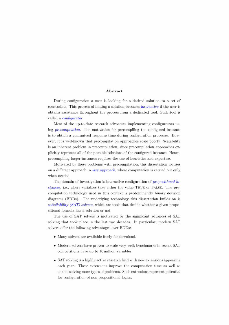
Abstract
During configuration a user is looking for a desired solution to a set of
constraints. This process of finding a solution becomes interactive if the user is
obtains assistance throughout the process from a dedicated tool. Such tool is
called a configurator.
Most of the up-to-date research advocates implementing configurators us-
ing precompilation. The motivation for precompiling the configured instance
is to obtain a guaranteed response time during configuration processes. How-
ever, it is well-known that precompilation approaches scale poorly. Scalability
is an inherent problem in precompilation, since precompilation approaches ex-
plicitly represent all of the possible solutions of the configured instance. Hence,
precompiling larger instances requires the use of heuristics and expertise.
Motivated by these problems with precompilation, this dissertation focuses
on a different approach: a lazy approach, where computation is carried out only
when needed.
The domain of investigation is interactive configuration of propositional in-
stances, i.e., where variables take either the value True or False. The pre-
compilation technology used in this context is predominantly binary decision
diagrams (BDDs). The underlying technology this dissertation builds on is
satisfiability (SAT) solvers, which are tools that decide whether a given propo-
sitional formula has a solution or not.
The use of SAT solvers is motivated by the significant advances of SAT
solving that took place in the last two decades. In particular, modern SAT
solvers offer the following advantages over BDDs:
• Many solvers are available freely for download.
• Modern solvers have proven to scale very well; benchmarks in recent SAT
competitions have up to 10 million variables.
• SAT solving is a highly active research field with new extensions appearing
each year. These extensions improve the computation time as well as
enable solving more types of problems. Such extensions represent potential
for configuration of non-propositional logics.

The goal of this dissertation is to show that SAT-based interactive configu-
ration does not suffer from scalability problems and it provides response times
that do not inconvenience the user. Moreover, the dissertation shows that the
SAT-based approach enables providing more informative explanations than the
precompiled approaches.
The main contributions of this dissertation are the following:
• algorithms to implement an interactive configurator using a SAT solver;
• algorithms to produce explanations for actions performed by the configu-
rator;
• an optimization that reduces the size of the given formula in the context
of interactive configuration and how to reconstruct explanations in the
context of such optimizations;
• a formalization of the completion of a configuration process and what it
means to make a choice for the user;
• an algorithm that helps the user to complete a configuration process with-
out making a choice for the user;
• a description of the design and implementation of the presented tech-
niques;
• an empirical evaluation of the implementation.

Typesetting Environments Several typesetting environments are used
throughout the text. The following conventions are used for them.
• Definitions are formal definitions of concepts used later in the text.
• Observations are facts that are very easy to prove or are obvious without
a proof.
• Lemmas are facts that are used to prove some other facts.
• Propositions are facts that may be important but are typically easy to
prove.
• Claims are substantial facts.
• Remarks are notes without which the surrounding text still makes sense.
They are aimed at giving to the reader more intuition of the discussed
material.
• Dings, marked with , are short, typically informal, conclusions of the
preceding text.
Chapter 1
Introduction
Computer users encounter configuration on daily basis. Whether when they
customize an application they use, customize how a new application is installed,
or just customize a query to a search engine. In all these cases the user picks
values from a set of choices and receives feedback when these choices are invalid.
And, in all these cases the underlying application or query is being configured.
Configuration can be done interactively or non-interactively. In the inter-
active case, the computer provides information about validity of choices each
time the user makes a new choice—this feedback typically takes the form of
graying out the choices that are no longer valid. In the non-interactive case, the
user first makes all the choices first and the computer checks the validity and
highlights the violations at the very end.
While non-interactive configuration is easier to implement for programmers,
interactive configuration is more user-friendly. It can be easily argued that fixing
a form after some fields have been marked as red (invalid) is far more tedious
than obtaining the feedback instantaneously.
A configurator is a tool that enables interactive configuration and it is in-
teractive configuration that is the main focus of this dissertation. In particular,
the focus is on the reasoning that a configurator has to perform in order to infer
which choices are valid and which are not.
The objective of this chapter is to familiarize the reader with the context of
configuration and with the basic principles used in configurators. In particular,
it discusses reuse (Section 1.1), modularization (Section 1.2, and software prod-
uct line engineering (Section 1.3). Section 1.4 presents a configurator from a
user perspective. To conclude the introduction, Section 1.5 discusses the moti-
vation and lists the main contributions of the dissertation. Section 1.7 outlines
the organization of the text.
2

1.1 Reuse
Software development is hard for many reasons: humans err, forget, have trouble
communicating, and software systems are larger than what one human brain
can comprehend. Researchers in Software Engineering try to help software
developers by looking for means that improve quality and efficiency of software
development. Reuse is one of these means and it is the main motivation for
configuration.
The basic idea of reuse is simple: developers use a certain product of their
work for multiple purposes rather than providing a new solution in each case.
This concept is not limited to source code. Artifacts that can be reused include
models, documentation, or build scripts. These artifacts are examples of a more
general class: programs written in a domain specific language (DSL) to produce
or generate other entities.
Let us briefly look at the main benefits of successful reuse. Firstly, it takes
less time to develop an artifact once than multiple times. Secondly, fixing, evolv-
ing or modifying an artifact is more efficient than fixing multiple occurrences
of it. Last but not least, code more used is code more tested, and, code more
tested is code more reliable.
There are several obstacles to reuse. A reusable piece of software needs
to provide more functionality than when it is developed for a single purpose.
Hence the developer must come up with a suitable abstraction of the software—
if the developer has not envisioned the future use of the software right, other
developers will not be able to reuse it.
Another obstacle is that if a developer writes software from scratch, it can
be expected that this developer understands it quite well. On the other hand,
reusing code developed by other people requires an investment into learning
about the artifacts to be reused. And, clearly: “For a software reuse technique
to be effective, it must be easier to reuse the artifacts than it is to develop the
software from scratch” [121]. Alas, to determine whether it is easier to develop
from scratch or to reuse is hard.
Frakes and Kang highlight several other issues with nowadays reuse [72]. One
issue is the scalability of reuse. Indeed, it is not always easy for a programmer to
find the right component for the activity in question if the component repository
is large. To address this problem a number of techniques have been proposed.
Such as semantic-based component retrieval [202], component rank [99], or by
providing information delivery systems that help programmers with learning
about new features [203]. Another problem highlighted by Frakes and Kang is
that state-of-the-practice means for describing components is insufficient. They
propose design by contract as an answer to this issue [149, 123]
3

1.2 Modularization
One important step toward reuse is modularization [56]. In a nutshell, modu-
larization is dividing artifacts (and the problem) into clearly defined parts while
inner workings of these parts are concealed as much as possible. For this pur-
pose, most mainstream programming languages provide means for encapsulation
and encapsulated components communicate via interfaces.
Modularization follows the paradigm of separation of concerns: it is easier
to focus on one thing than on many at the same time (human brain has limited
capacity). At the same time, modularization facilitates reuse by making it easier
to determine the portion of an existing artifact that needs to be reused in order
to obtain the desired functionality.
Software engineers, when writing modularized code, deal with an inherent
problem: how to describe an artifact well without relying on its inner workings?
In other words, devising component interfaces is difficult. Mainstream high-level
languages (C-family, ML family) provide syntax-based interfaces embellished
with type-checking. Such interfaces typically do not carry enough information
for the component to be usable. Hence, natural language documentation is an
imperative.
Natural language documentation, however, is not machine-readable and thus
it cannot be used for reasoning about the component nor it is possible to auto-
matically check whether the implementation fulfills the documentation. Logic-
based annotations try to address this issue. Indeed, languages like Java Mod-
eling Language (JML) [123] are a realization of Floyd-Hoare triples [96]. The
research in this domain is still active and to this date the approach has not
achieved a wide acceptance.
To conclude the discussion on modularization we should note that the
concept of a module differs from language to language. Many researchers
argue that the traditional approaches to modularization are weak when it
comes to orthogonal separation of concerns. Feature Oriented Program-
ming (FOP) [168, 17, 16, 129] and Aspect oriented programming (AOP) [117]
are examples of approaches to orthogonal modularization at the source-code
level.
1.3 Software Product Line Engineering
Software Product Line Engineering (SPLE) [39] is a Software Engineering ap-
proach which tries to improve reuse by making it systematic. More specifically, a
software product line (or just product line) is a system for developing a particu-
lar set of software products while this set is explicitly defined. A popular means
4

for defining such set are feature models, which are discussed in Section 2.4. This
set needs to comprise products that are similar enough for the approach to be
of value. For this purpose we use the term program families, defined by Parnas
as follows.
. . . sets of programs whose common properties are so extensive
that it is advantageous to study the common properties of the pro-
grams before analyzing individual members. [165]
With a bit of imagination, program families appear even in single-product
development as eventually any successful single program ends up having several
versions. In SPLE, however, the family of products to be targeted is defined
up front and is explicitly captured in variability models. The name variability
models comes from the fact that such model must capture how the products in
the family differ from one another. Analogously, properties shared among the
products form the commonality1. The analysis concerned with determining the
variability model is called domain analysis.
The motivation for deciding on the product family beforehand is so that the
individual products can be manufactured with minimal effort. An individual
product of the family is developed with the reuse of core assets — a set of
artifacts that is to be reused between members of the family. In the ideal case,
products are assembled only using the core assets with little additional work
needed. The construction toy Lego is a popular metaphor for this ideal case:
The individual Lego pieces are core assets reused to obtain new constructs.
Variability models and the set of pertaining potential products are often
generalized to the concepts of problem space and solution space [44]. Problem
space is formed by descriptions of the products that might or should be devel-
oped and solution space by potential implementations of products. In terms of
these concepts, a task of a product line is to map elements of problem space
to elements of solution space (see Figure 1.1). Figure 1.1 shows the role of a
Problem space Solution space
valid problem or solution invalid problem or solution
Figure 1.1: Concepts in a product line
variability model in a product line: the rectangles represent whole spaces, the
1Admittedly, these terms are typically defined vaguely.
5
ellipses represent parts of the determined by the model. The model determines
a set of valid products, which is a subset of a larger space.
To relate to our Lego example, the pieces enable us to assemble all sorts
of constructions but we are probably interested only in those that do not keel
over. Analogously, typically only a subset of the problem space is considered.
We might, for example, require that we are only interested in those compositions
of core assets that compile.
A software product line connects a solution space and a problem space;
the valid set of problems is explicitly defined by a variability model.
We should note that often solution and problem space are in a 1-to-1 relation-
ship and the distinction between them is not immediately clear. For instance,
a core asset repository may contain a component Optimizer that provides the
optimization functionality. The functionality is part of the problem space (Do
we want an optimized product?) while the component belongs into the solution
space. The distinction would have been more apparent if we had components
OptimizerA and OptimizerB both providing the optimization functionality. A
formalization of the relation between the two spaces is found in [104].
SPLE is a systematic approach to reuse which explicitly defines the set
of potential products.
1.4 A Configurator from the User Perspective
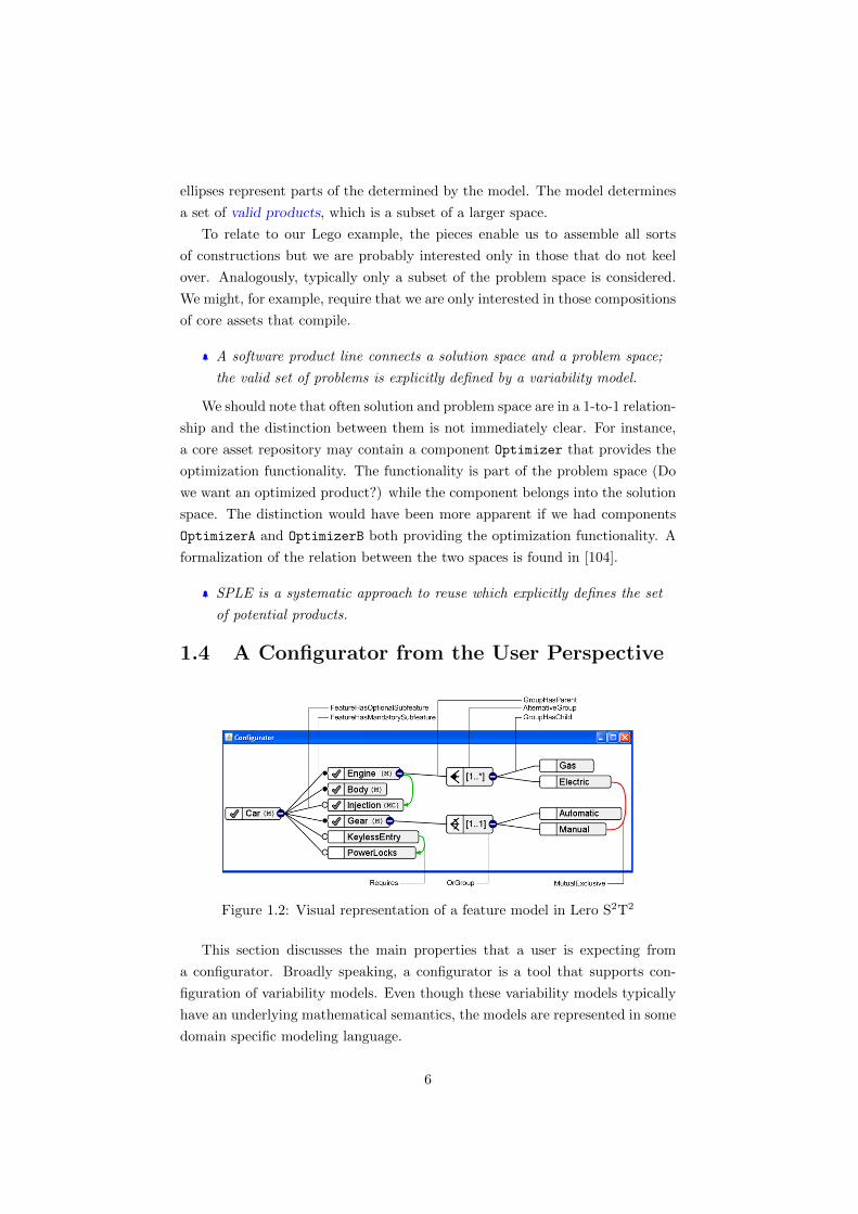
Figure 1.2: Visual representation of a feature model in Lero S2T2
This section discusses the main properties that a user is expecting from
a configurator. Broadly speaking, a configurator is a tool that supports con-
figuration of variability models. Even though these variability models typically
have an underlying mathematical semantics, the models are represented in some
domain specific modeling language.
6
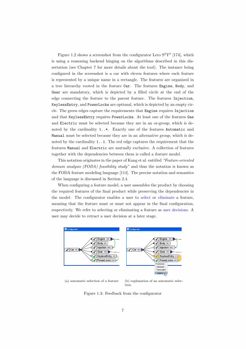
Figure 1.2 shows a screenshot from the configurator Lero S2T2 [174], which
is using a reasoning backend hinging on the algorithms described in this dis-
sertation (see Chapter 7 for more details about the tool). The instance being
configured in the screenshot is a car with eleven features where each feature
is represented by a unique name in a rectangle. The features are organized in
a tree hierarchy rooted in the feature Car. The features Engine, Body, and
Gear are mandatory, which is depicted by a filled circle at the end of the
edge connecting the feature to the parent feature. The features Injection,
KeylessEntry, and PowerLocks are optional, which is depicted by an empty cir-
cle. The green edges capture the requirements that Engine requires Injection
and that KeylessEntry requires PowerLocks. At least one of the features Gas
and Electric must be selected because they are in an or-group, which is de-
noted by the cardinality 1..*. Exactly one of the features Automatic and
Manual must be selected because they are in an alternative group, which is de-
noted by the cardinality 1..1. The red edge captures the requirement that the
features Manual and Electric are mutually exclusive. A collection of features
together with the dependencies between them is called a feature model.
This notation originates in the paper of Kang et al. entitled “Feature-oriented
domain analysis (FODA) feasibility study” and thus the notation is known as
the FODA feature modeling language [114]. The precise notation and semantics
of the language is discussed in Section 2.4.
When configuring a feature model, a user assembles the product by choosing
the required features of the final product while preserving the dependencies in
the model. The configurator enables a user to select or eliminate a feature,
meaning that the feature must or must not appear in the final configuration,
respectively. We refer to selecting or eliminating a feature as user decisions. A
user may decide to retract a user decision at a later stage.
(a) automatic selection of a feature (b) explanation of an automatic selec-tion.
Figure 1.3: Feedback from the configurator
7

A configurator prevents the user from making invalid choices, choices
that would violate the feature model, by automatically selecting or elimi-
nating features. For instance, in Figure 1.3a the user has selected the fea-
ture KeylessEntry and the configurator automatically selected the feature
PowerLocks since the car cannot have KeylessEntry without PowerLocks.
In some cases, the user wants to know why a certain feature was automat-
ically selected or eliminated. A piece of information showing why a certain
automatic choice was made is called an explanation. An example of a situation
where an explanation is useful is when the user wants to select a certain fea-
ture but that is not possible because that feature was automatically eliminated.
Then, the user can change the choices that led to the automatic elimination of
that feature. Analogously, the user might want to eliminate a certain feature
but that is not possible because it has been automatically selected.
Figure 1.3b depicts an example of an explanation. In this example the
user has asked why power-locks were automatically selected. The configurator
highlights the requires edge between KeylessEntry and PowerLocks, and, the
user decision to select KeylessEntry. We can imagine, for example, that the
user does not want PowerLocks because they are too expensive. The explana-
tion, however, shows to the user that KeylessEntry cannot be selected without
PowerLocks. Then, the user might either decide to pay for the PowerLocks or
sacrifice KeylessEntry, i.e., eliminate the feature KeylessEntry.
Note that by automatically eliminating or selecting certain features the con-
figurator effectively disallows certain user decisions. If the feature had been
automatically eliminated, the user cannot select the feature and vice versa.
Configurators may differ in which user decisions they disallow. The focus of
this dissertation is a configurator that is backtrack-free and complete.
Backtrack-freeness means that if the user is making only allowed decisions
then it will always be possible to complete the configuration without retracting
some decisions (without backtracking). Completeness of a configurator means
that the configurator disallows only decisions that are necessary to disallow. In
other words, any feature configuration permitted by the feature model is reach-
able by a sequence of allowed user decisions in a complete configurator. Both
of these concepts, backtrack freeness and completeness, are defined formally in
Section 3.1.
Configuration does not have to be limited to feature models. Nor do the
user decisions have to be limited to selection and elimination. For instance,
the configurator may support numerical variables and user decisions that affect
their values. In this dissertation, however, the primary focus is a configuration
supporting selections and eliminations. The interested reader is referred to the
chapter concerned with the related work for further references on configuration
8

of other types of constraints (Chapter 10).
1.5 Motivation and Contributions
The majority of research on configuration hinges on precompilation. In pre-
compilation the instance to be configured is precompiled into a specialized data
structure, which enables implementing a configurator with guaranteed response
time [3]. In propositional interactive configuration, which is the focus of this
dissertation, the data structure predominantly used for precompilation is binary
decision diagrams (BDDs) [92, 89, 5, 196, 93, 94].
In contrast to precompilation, the approach presented in this dissertation
is a lazy approach—no precompilation is required as all the computation takes
place as the configuration proceeds.
There are two main arguments for researching the lazy approach: scalability
and informativeness of explanations. It is well-known that BDDs are difficult to
construct for instances with more than hundreds of variables [1, 23]. The reason
for poor scalability of BDDs is the fact that a BDD is an explicit representation
of all the satisfying assignments of the pertaining formula. Since the number
of satisfying assignments of a formula grows exponentially with the number of
variables, it is easy to encounter formulas whose BDD representation is beyond
the capacities of modern computers [33]. Moreover, finding a BDD that is
optimal in size is hard [26]. Consequently, precompilation of large instances
requires heuristics specific to the instance. Clearly, this is highly impractical for
laymen users.
The problem of scalability of precompilation is inherent because precom-
pilation explicitly represents all the solutions of the configured instance, and,
the number of solutions typically grows exponentially with the number of vari-
ables. A number of researchers propose a variety of heuristics and modifica-
tions of the data structures for precompilation in order to deal with scalabil-
ity [136, 164, 189, 187, 188, 148]. While some of these heuristics and approaches
may succeed for a particular instance, some may not. This poses a significant
technological barrier: the user has to experiment with the different approaches
to see which work, and, these techniques are often intricate and therefore not
easy to implement. We argue that the SAT approach scales uniformly , i.e.,
there is no need for heuristics for specific instances. Additionally, from an engi-
neering perspective, the use of a SAT solver as the underlying technology is an
advantage because many SAT solvers are freely available and new ones appear
each year. The research in SAT solving is propelled by the yearly SAT com-
petitions [176, 177]. In contrast to that, BDD libraries are scarce and the last
known comparative study of BDD libraries is from the year 1998 [201].
9

The second argument for our approach is that precompilation methods have
limited capabilities when it comes to explanations. Again, this problem is in-
herent because the structure of the instance that is to be configured is lost in
the precompiled data structure, i.e., the mapping from formulas to BDDs is not
injective. Even though there exists work on providing proofs using BDDs, it is
not clear how explanations would be constructed from these proofs (see Chap-
ter 9 for further discussion). Consequently, the BDD-based approaches provide
only explanations as sets of user decisions. In contrast to that, in our approach
we provide not only the user decisions but also the parts of the configured in-
stance and dependencies between them. We argue that this adds significant
value to the explanations because in order to understand why a certain choice
was disabled, the user needs to take into account the configured instance.
Hence, the main contribution of this dissertation is a demonstration of the
advantages of the SAT-based approach to implementing interactive configura-
tion over the precompilation-based approach. The particular contributions are
the following:
• Chapter 4 describes algorithms for implementing a configurator using a
SAT solver and Section 4.5 describes algorithms for constructing explana-
tions from resolution trees obtained from the solver.
• Chapter 5 shows how to integrate into a configurator a syntactic-based
optimization and how to reconstruct proofs in the presence of this opti-
mization.
• Chapter 6 formalizes what it means to “make a choice for the user” and
Section 6.3 presents an algorithm for computing variables that can be
eliminated without making a choice for the user.
• Chapter 7 describes a design of the implemented configurator, which sug-
gests design patterns that other programmers could find useful in imple-
menting configurators.
• Chapter 8 empirically evaluates the presented algorithms and shows the
impact of the different optimizations.
1.5.1 Comparison to State-of-the-Art
Interactive Configuration
Even though some aspects of the lazy approach are addressed in the existing re-
search literature, a thorough study of the subject is missing. Kaiser and Kuchlin
propose an algorithm for computing which variables must be set to True and
10

which to False in a given formula [113]. This is, in fact, a sub-problem of
propositional interactive configuration, as in interactive configuration, the for-
mula effectively changes as the user makes new decisions. Additionally to the
work of Kaiser and Kuchlin, this dissertation shows how to take advantage of
the computations made for the previous steps of the configuration process.
The basic ideas behind the presented algorithms is captured in an earlier
article of mine [103]. The works of Batory and Freuder et al. provide algorithms
for providing lazy approach to interactive configuration [79, 77, 15]. The work of
Freuder et al. is in the context of constraint satisfaction problems (CSPs) [79, 77]
while the work of Batory is in the context of propositional configuration [15].
Even though the approaches are lazy, as the one presented in this dissertation,
they do not satisfy the requirements of completeness and backtrack-freeness.
Informally, completeness is when the user can reach all possible solutions and
backtrack-freeness is when the configurator allows only such sequences of user
decisions that can be extended into a solution (these concepts are formally
defined in Chapter 3 and the above-mentioned articles are discussed in greater
detail in Chapter 10).
The approach of Batory is inspired by truth maintenance systems [52, 69],
in particular by logic truth maintenance systems (LTMSs). An LTMS is a
helper-component for algorithms that traverse a state space in order to find a
solution; such traversal may be carried out by backtracking, for instance. One
role of an LTMS is to identify if the search reached a conflict, i.e., identify that
the traversing algorithm is in a part of the state space that does not contain
a solution. The second role is to identify parts of the state space that should
not be traversed because they do not contain a solution; this is done by unit
propagation (see Section 2.1.3). In Batory’s approach it is not an algorithm
that traverses the state space, but it is the user who does so. However, the role
of the LTMS remains the same.
An LTMS is implicitly contained in our approach because a SAT solver per-
forms unit propagation in order to prune the state space2 (see Section 2.3). On a
general level, an interactive configurator satisfies the interface of an LTMS. How-
ever, guaranteeing backtrack-freeness is as computationally difficult as finding a
solution (see Section 4.3.2). Hence, using a backtrack-free interactive configura-
tor as a component for an algorithm that is looking for a solution in the search
space is not practical.
Finally, we note that the lazy approach to configuration also appears in
configuration of non-discreet domains. Indeed, it is unclear how to precom-
2Modern SAT solvers do not use an LTMS as a separate component but instead tie theimplementation of the functionality of an LTMS with the search algorithm. This enables amore efficient implementation of the functionality because the order of the traversal is known.
11

pile configuration spaces with infinite numbers of solutions. Compared to our
problem domain (propositional configuration), non-discreet domains are sub-
stantially different. Hence, the underlying technology has to be substantially
different as well. In particular, the technology used in the reviewed literature
are procedures from linear programming [131, 90].
Explanations
The algorithms constructing explanations from resolution trees (Section 4.5) are
novel as the surveyed literature only shows how to provide explanations as sets
of user decisions in backtrack-free and complete configurators. Interestingly
enough, the explanations provided in non-backtrack-free approaches are also
resolution trees [79, 15]. However, since these algorithms are profoundly differ-
ent from those presented in this dissertation, their mechanism of explanations
cannot be reused (see also Section 4.5.3 for further discussion).
Syntactic Optimization
The syntactic optimization (BIS-optimization) proposed in Chapter 5 is not
novel. Indeed, it is well-known in the SAT community that the computation of
satisfiability can be optimized using this technique (see Section 10.2 for further
details). However, that are two main contributions that this dissertation makes
in the context of this optimization.
The first contribution is our novel manner of application. Applying the BIS-
optimization at the level of a SAT solver and at the level of a configurator is
not the same. In particular, it does not yield the same effect—as the config-
urator calls the solver multiple times, the optimization has greater effect than
if it were applied individually whenever the solver is called. Hence, the opti-
mization is applied in a different fashion than in SAT solving. Moreover, the
same effect achieved by the proposed technique cannot be achieved by adding
the optimization to the underlying solver (see Remark 5.21 for further details).
The second contribution in regards to the BIS-optimization is proof recon-
struction. The surveyed literature does not contain any work on how to recon-
struct resolution trees obtained from a solver that operates on the optimized
formula (which is needed to provide explanations). Additionally, we provide a
heuristic that aims at minimizing the size of the reconstructed tree. Since the
empirical evaluation shows that this heuristics significantly reduces the size, this
serves as motivation for studying similar heuristics for other types of syntactic
optimizations.
12

Configuration Process Completion
The formalization of the concept “making a choice for the user” appears in an
earlier article of mine [105] and does not appear in any other surveyed litera-
ture. Compared to that article, the definition presented in this dissertation is
improved for clarity and intuition (the concepts of choice were not explicit in the
earlier definitions). More importantly, the dissertation shows how to calculate
variables that can be eliminated without making a choice for the user.
Implementation
The described architecture of the implemented configurator (Chapter 7) is the
well-known pipe-and-filter architecture and also bears some characteristics of
the GenVoca approach [18], as the translation from a modeling language to a
logic language is performed in a chain of smaller steps (in GenVoca these steps
are called layers). However, there are some particularities in the design—mainly,
in the way how explanations are dealt with. In order to enable explanations,
the configured instance is not treated as a whole, but as a set of primitives, and
the components realizing the translation from a modeling language to a logic
language need to communicate in both directions.
The dissertation studies a lazy approach to interactive configuration—an
approach in which computation is done only when needed. The underly-
ing technology for realizing this approach are modern satisfiability (SAT)
solvers.
1.6 Thesis Statement
SAT solvers and BDDs are two predominant alternative means for solving propo-
sitional problems. BDDs were invented in 1986 by Bryant [34] and celebrated a
great success in model checking in the early 90s [35, 144]. Efficient SAT solvers
started to appear somewhat later, i.e., in the late 90s [138, 139, 204, 158].
Shortly after that, SAT solvers were successfully applied in various do-
mains [181, 183, 25, 14, 128, 154, 59, 53, 28]. In particular, it has been shown
that in model checking SAT solvers do not suffer from scalability issues as BDDs
do [23, 1].
These success stories of SAT solvers served as the main motivation for this
dissertation: investigate how SAT solvers can be applied in the context of inter-
active configuration. This direction of research is further encouraged by recent
work by Mendonca et al. who show that SAT solving in the context of feature
models is easy despite the general NP-completeness of the problem [147].
13

While interactive configuration has been mainly tackled by BDD-based ap-
proaches, this dissertation argues that SAT-based approach scales better and
enables more informative explanations. Hence, the outlined arguments lead to
the following thesis statement.
SAT solvers are better for implementing a Boolean interactive con-
figurator than precompiled approaches.
1.7 Outline
The dissertation is divided into the following chapters. Chapter 2 introduces
notation and terms that are used in the dissertation. This chapter can be
skipped and used as a back reference for the other chapters.
Chapter 3 puts configuration in a formal context and derives several im-
portant mathematical properties related to configuration. These properties are
used by Chapter 4 to construct a configurator using a SAT solver. Chapter 5
proposes an optimization that is based on processing the instance to be config-
ured; several important issues regarding explanations are tackled.
Chapter 6 studies how to help the user to complete a configuration process
without making a choice for the user. An implementation of the proposed
technique using a SAT solver is described.
Chapter 7 describes the design of the configurator that was implemented
using the presented algorithms. The chapter discusses how a feature model is
represented and the architecture is organized.
Chapter 8 presents measurements that were performed on several sample
instances. The response time of the computation is reported and discussed.
Additionally, for the technique that is designed to help the user to complete a
configuration it is reported how efficient it is.
Chapter 10 overviews the related work and Chapter 11 concludes the disser-
tation.
14

Chapter 2
Background
This chapter serves as a quick reference for background material of this dis-
sertation. Section 2.1 overviews general computer science terms. In particular
Section 2.1.6 lists the notation used throughout the dissertation. Section 2.2 ref-
erences the technology that can be used to implement the algorithms presented
in the dissertation. Section 2.3 describes the main principles behind modern
SAT solvers. Section 2.4 defines the notation and semantics for feature models
that are used as instances for configuration.
2.1 General Computer Science
2.1.1 Propositional Logic
Most of the text in this thesis operates with propositional logic with standard
Boolean connectives (∧,∨,⇒,⇔) and negation (¬) with their standard meaning.
The names of propositional variables are typically lower-case letters taken from
the end of the alphabet.
For a set of Boolean variables, a variable assignment is a function from
the variables to {True,False}. A variable assignment is often represented as
the set of variables that are assigned the value True, the other variables are
implicitly False. A model of a formula φ is such a variable assignment under
which φ evaluates to True (a model can be seen as a solution to the formula).
Example 1. The formula x ∨ y has the models {x}, {y}, and {x, y}. The
assignment ∅, which assigns False to all variables, is not a model of x ∨ y.
An implication x⇒ y corresponds to the disjunction ¬x∨y. For the implica-
tion x⇒ y, the implication ¬y⇒¬x is called its contrapositive. An implication
and its contrapositive are equivalent (the sets of models are the same).
15

A formula is satisfiable iff there is a assignment of the variables for which
the formula evaluates to True (the formula has a model); a formula is unsatis-
fiable iff it is not satisfiable. If a formula evaluates to True under all variable
assignments then it is called a tautology. For instance, x∨y is satisfiable, x∧¬xis unsatisfiable, and x ∨ ¬x is a tautology. We say that the formulas ψ and φ
are equisatisfiable iff they are either both satisfiable or both unsatisfiable.
We write ψ |= φ iff φ evaluates to True under all variable assignments
satisfying ψ, e.g., x ∧ y |= x. We write ψ 2φ if there is a variable assignment
under which ψ is True and φ is False. Note that for any tautology φ, it holds
that True |= φ and for any formula ψ it holds that False |= ψ.
2.1.2 Minimal Models
A model of a formula φ is minimal iff changing a value from True to False for
any subset of the variables yields a non-model. When models are represented as
sets of values whose value is True, then changing a value from True to False
corresponds to removing the variable from the model. Therefore a model M of
φ is minimal iff any proper subset of M is not a model of φ.
We write M(φ) to denote the set of all minimal models of φ. We write
φ |=min ψ to denote that ψ holds in all minimal models of φ.
Example 2. The formula φdef= x∨y has the models {x}, {y}, {x, y}. The model
{x, y} is not a minimal model of x ∨ y because removing either x or y yields a
model. However, removing x from {x} yields ∅, which is not a model of φ and
therefore {x} is a minimal model of φ. Analogously, {y} is a minimal model.
ThereforeM(x∨ y) = {{x}, {y}}. Since {x, y} is not a minimal model, it holds
that x ∨ y |=min ¬(x ∧ y).
{x, y}
{x} {y}
∅( (
( (
x∨y
M(x∨y)
The different sets of variables form a lat-
tice ordered by the subset relation. Mod-
els of a particular formula are a subset of
that lattice (the outer rectangle). The min-
imal models are the smallest elements in
that subset (the inner rectangle).
Figure 2.1: Ordering on models
Figure 2.1 gives another insight into the concept of minimal models. The
subset relation defines an ordering where the empty set is the smallest element
and the set of all the considered variables the largest. Minimal models are the
minimal elements of this ordering on the models of the formula in question.
Minimal models are used in Chapter 6 in order to find variables that can
16

be set to False without making a choice for the user (see Definition 16). In
particular, we will look for variables that have the value False in all minimal
models (see Section 6.3).
2.1.3 Conjunctive Normal Form (CNF)
A propositional formula is called a literal iff it is a variable or a negated variable
(e.g., ¬v). A formula is called a clause iff it is a disjunction of zero of more literals
(e.g., ¬v∨w, ¬x). Each variable must appear at most once in a clause. A formula
is in the conjunctive normal form (CNF) iff it is a conjunction of clauses, e.g.,
(¬v ∨w)∧ (¬x). For a literal l, we write l to denote the complementary literal,
i.e., if l ≡ x then ldef= ¬x; if l ≡ ¬x then l
def= x.
The notion of literal and clause is of particular importance for understanding
the dissertation.
When a formula is in CNF, it is often treated as a set of clauses (implicitly
conjoined). Analogously, a clause can be seen as literals (implicitly disjoined).
However, clauses are typically written as disjunctions.
Special forms of clauses The empty clause, i.e., clause containing no literals,
is denoted as ⊥ and is logically equivalent to False. A clause comprising one
literal is called a unit clause. Any implication l⇒ k where l and k are literals,
corresponds to the clause l∨ k. Therefore, we write such implications in a CNF
formula whenever suitable.
A clause c1 is subsumed by the clause c2 iff the set of literals of c2 is a
subset of the literals of c1 (e.g., x subsumes x ∨ y). If a set of clauses contains
such two clauses, removing c1 yields an equisatisfiable formula, e.g., (x ∨ y) ∧ xis equisatisfiable with x. (Moreover, any satisfying assignment of x can be
extended to a satisfying assignment of (x ∨ y) ∧ x by assigning an arbitrary
value to the variable y.)
Resolution
Two clauses c1 and c2 can be resolved if they contain at least one mutually
complementary literal. To resolve such c1 and c2 means to join the clauses while
omitting the literal and its complement. More precisely, for clauses comprised
of the sets of literals c1 and c2, respectively, such that l ∈ c1 and l ∈ c2 for some
variable v that {v,¬v} = {l, l}, resolution over the variable v yields a clause
comprising the literals c1 ∪ c2 \ {v,¬v}. The result of resolution is called the
resolvent. For instance, resolving x ∨ y and x ∨ ¬y yields the resolvent x.
A resolution of two clauses for which at least one is a unit clause is called a
17

unit resolution. Performing unit resolution exhaustively is called unit propaga-
tion.
Example 3. Unit propagation on the clauses {p,¬p ∨ q,¬q ∨ x} yields the set
{p,¬p ∨ q,¬q ∨ x, q, x}. Since ¬p ∨ q is subsumed by q and ¬q ∨ x is subsumed
by x, the following set of clauses is equisatisfiable {p, q, x}.
Proving by Resolution
In logic in general, proofs are carried out from a theory where a theory is a set
of formulas. Since any CNF formula is a set of clauses, i.e., smaller formulas,
the difference between a theory and a formula is only conceptual. Hence, in this
dissertation CNF formulas are treated as theories whenever needed.
We say that ψ is proven from φ by resolution if ⊥ is derived from φ∧¬ψ by
a finite number of applications of the resolution rule; we write φ ` ψ if that is
the case.
The resolution rule is a sound inference rule, i.e., if r is a resolvent of c1 and
c2, it holds that c1∧ c2 |= r. Resolution is complete with respect to consistency,
i.e., ψ is unsatisfiable (inconsistent), if and only if ⊥ can be derived from ψ by a
finite number of applications of the resolution rule. Consequently, the resolution
proof system is sound and complete, i.e., φ ` ψ if and only if φ |= ψ.
A set of resolutions deriving ⊥ from a formula φ form a tree with some of the
clauses from φ as leaves and ⊥ as the root; we refer to such tree as resolution
tree. We say that such tree refutes φ.
Example 4. Let φ be ((x ∧ y)⇒ z) ∧ x ∧ (¬y ∨ ¬z), then φ ` ¬y. To show
that φ ` ¬y, we refute φ ∧ y. This refutation is realized by the resolution
tree in Figure 2.2. Note that resolution trees are typically drawn upside down
compared to trees in general.
Remark 2.2. The graph in Figure 2.2 is rather a directed acyclic
graph (DAG) than a tree because some clauses are used in multiple
resolution steps. Nevertheless, the graph can be redrawn as a tree if
all these clauses are duplicated each time they are used. We mostly
use the DAG representation since it is more compact but we continue
using the term tree.
Remark 2.3. Resolution can generalized to formulas in first order
logic but this is not used in this dissertation. For details on resolution
see [132].
Example 5. Figure 2.3 presents three common patterns of resolution. (1) Re-
solving x with x⇒ z yields z because x⇒ z is equivalent to ¬x ∨ z. In general,
18
¬x ∨ ¬y ∨ z x y ¬y ∨ ¬z
¬y ∨ z1 1
z2
2
¬y3
3
⊥4
4
An example of a resolution tree
where the edges are labeled with
the number of the pertaining reso-
lution step, e.g., the resolution of
y and ¬y which yields ⊥ is the
last (fourth) step.
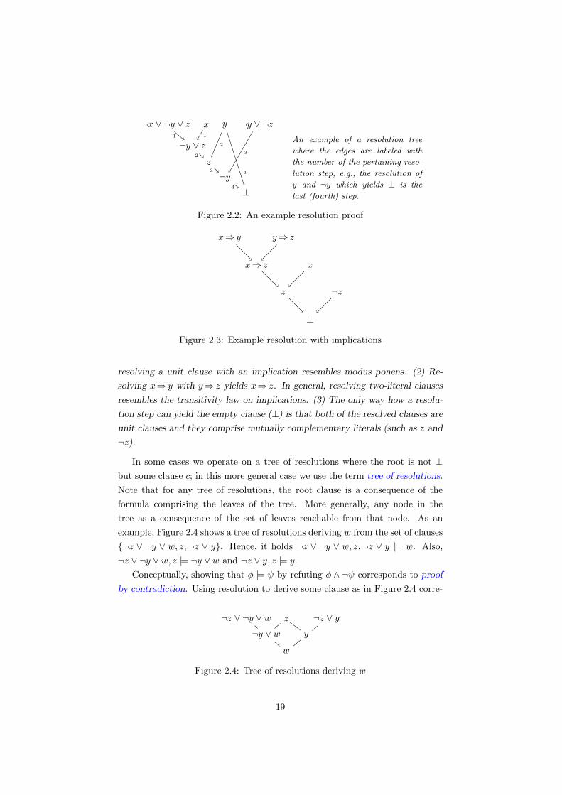
Figure 2.2: An example resolution proof
⊥
¬zz
x⇒ z x
x⇒ y y⇒ z
Figure 2.3: Example resolution with implications
resolving a unit clause with an implication resembles modus ponens. (2) Re-
solving x⇒ y with y⇒ z yields x⇒ z. In general, resolving two-literal clauses
resembles the transitivity law on implications. (3) The only way how a resolu-
tion step can yield the empty clause (⊥) is that both of the resolved clauses are
unit clauses and they comprise mutually complementary literals (such as z and
¬z).
In some cases we operate on a tree of resolutions where the root is not ⊥but some clause c; in this more general case we use the term tree of resolutions.
Note that for any tree of resolutions, the root clause is a consequence of the
formula comprising the leaves of the tree. More generally, any node in the
tree as a consequence of the set of leaves reachable from that node. As an
example, Figure 2.4 shows a tree of resolutions deriving w from the set of clauses
{¬z ∨ ¬y ∨ w, z,¬z ∨ y}. Hence, it holds ¬z ∨ ¬y ∨ w, z,¬z ∨ y |= w. Also,
¬z ∨ ¬y ∨ w, z |= ¬y ∨ w and ¬z ∨ y, z |= y.
Conceptually, showing that φ |= ψ by refuting φ ∧ ¬ψ corresponds to proof
by contradiction. Using resolution to derive some clause as in Figure 2.4 corre-
w
¬y ∨ w¬z ∨ ¬y ∨ w z
y
¬z ∨ y
Figure 2.4: Tree of resolutions deriving w
19

sponds to traditional proof by deduction. The reason why proof by contradiction
is used with resolution is that resolution is not complete for deduction but only
for contradiction. For instances, there is no way how to show x |= x ∨ y by
applying the resolution rule to the clause x. However, it is possible to refute
x ∧ ¬x ∧ ¬y.
CNF and complexity
To determine whether a CNF formula is satisfiable or not is NP-complete [41].
However, even though deciding whether a formula is a tautology is in general
co-NP-complete, a CNF formula is a tautology if and only if it comprises only
clauses that contain a literal and its complement, which can be detected in
polynomial time.
Converting to CNF
Any formula can be equivalently rewritten into CNF using De Morgan laws.
This may, however, cause an exponential blow-up in the size of the formula. For
instance, applying De Morgan’s laws to the formula (x1 ∧ y1) ∨ · · · ∨ (xn ∧ yn)
results into 2n clauses each having n literals.
Nevertheless, it is possible to transform any formula into a CNF formula
which is equisatisfiable and linear in the size of the original one by using Tseitin
transformation [192].
Tseitin transformation adds new variables to represent subformulas and adds
clauses to record the correspondence between these variables and the subformu-
las. Here we show Tseitin transformation for a language with ¬, ∧, and ∨. The
reader is referred for example to a monograph by Bradley and Manna for further
details [31].
Let R(φ) be a variable representing the subformula φ where each variable
in the original formula is represented by itself (R(v) = v) while all the other
representative variables are fresh. For the formula φ ≡ ψ ∧ ξ add the clauses
R(φ)⇒R(ψ), R(φ)⇒R(ξ), and (R(ψ) ∧ R(ξ))⇒R(φ). For the formula φ ≡ψ ∨ ξ add the clauses R(φ)⇒(R(ψ) ∧ R(ξ)), R(ψ)⇒R(φ), and R(ξ)⇒R(φ).
For the formula φ ≡ ¬ψ add the clauses R(φ)⇒¬R(ψ) and ¬R(ψ)⇒R(φ).
Finally, to assert that the formula must hold, add the clause R(φ) where φ is
the whole formula being encoded.
Example 6. Consider the formula (x1 ∧ y1) ∨ · · · ∨ (xn ∧ yn). For each term
xi ∧ yi introduce an auxiliary variable ri and generate the clauses ¬ri ∨ xi ∨yi,¬xi∨ri,¬yi∨ri. Together with these clauses an equisatisfiable representation
of the original formula in CNF is r1 ∨ · · · ∨ rn.
20

Although Tseitin transformation preserves satisfiability, some properties it
does not preserve. One particular property not preserved by the transformation
is the set of minimal models as shown by the following example.
Example 7. Let φ ≡ ¬x∨z and let n be the variable representing ¬x and f be
the variable representing φ. The Tseitin transformation results in the following
set of clauses.f⇒(n ∨ z) x ∨ nn⇒ f ¬x ∨ ¬nz⇒ f f
While φ has the only minimal model ∅, i.e., assigning False to both x and z,
the transformed formula has the minimal models {f, n} and additionally the
minimal model {f, z, x}.
2.1.4 Constraint Satisfaction Problem (CSP)
Most of the text of this dissertation deals with propositional logic. This section
discusses several basic concepts from constraint satisfaction programming, which
are referenced mainly in the related work section.
Definition 1 (CSP). A CSP is a triple 〈V, D, C〉 where V is a set of variables
V = {v1, . . . , vn}, D is a set of their respective finite domains D = {D1, . . . , Dn}.The set C is a finite set of constraints. A constraint C ∈ C is a pair 〈VC , DC〉where VC ⊆ V is the domain of the constraint and DC is a relation on the
variables in VC , i.e., DC ⊆ Di1 × · · · ×Dik if VC = {vi1 , . . . , vik}.A variable assignment is an n-tuple 〈c1, . . . , cn〉 from the Cartesian product
D1× · · · ×Dn, where the constant ci determines the value of the variable vi for
i ∈ 1 . . . n.
A variable assignment is a solution of a CSP if it satisfies all the constraints.
For an overview of methods for solving CSP see a survey by Kumar [122].
Arc Consistency A CSP is arc consistent [74] iff for any pair of variables and
any values from their respective domains these values satisfy all the constraints
on those variables. The term arc comes from the fact that we are ensuring that
for any pair of values there is an “arc” between them that records the fact that
this pair of values satisfies the pertaining constraints.
Arc consistency can be achieved by removing values from domains of vari-
ables as illustrated by the following example.
Example 8. Let us have a CSP with variables x1 and x2 and their respective
domains D1def= {1} and D2
def= {0, 1}. And let us consider the constraint {〈1, 1〉}
which enforces both variables to be 1.
21

The CSP is not arc consistent because the value 0 for x2 never satisfies the
constraint. However, removing 0 from its domain yields an arc consistent CSP.
The algorithm AC-3 reduces domains of variables in order to achieve arc
consistency in time polynomial to the size of the problem [135].
Remark 2.4. Arc consistency is in fact a special case of k-
consistency [74], which takes into account k variables; arc consistency
is k-consistency for k = 2. If a problem is k-consistent for k equal
to the number of variables of the CSP, then for each domain and
a value there exists a solution of the CSP using that value. Any k
less than that does not guarantee this property. Nevertheless, ensur-
ing k-consistency removes values that are certainly not used in any
solution [74].
2.1.5 Relation between CSP and Propositional Logic
Any propositional formula can be expressed as a CSP by considering all the
variable domains to be {False,True}.
Example 9. Let us have the variables x, y, z, and the formula (x⇒ y) ∧(y⇒ z). The formula can be expressed as the two following constraints each
corresponding to one of the implications.
c1def= 〈{x, y}, {〈False, False〉 , 〈False, True〉 , 〈True, True〉}〉
c2def= 〈{y, z}, {〈False, False〉 , 〈False, True〉 , 〈True, True〉}〉
If arc consistency is combined with node consistency—a requirement that no
value violates any unary constraint—then it is equivalent to unit propagation
on 2-literal clauses (see Section 2.1.3) as illustrated by the following example.
Example 10. Consider again the formula in the example above (Example 9)
represented as a CSP but now with the additional unary constraint requiring x
to be True.
Since the value False violates the unary constraint, it is removed from the
domain of x. Consequently, the constraint on x and y will be pruned to contain
only 〈True, True〉 and the value False will be removed from the domain of y
(see below). Analogously, False will be removed from the domain of z.
x
True
x y
((((((hhhhhhFalse False
((((((hhhhhhFalse True
True True
y z
((((((hhhhhhFalse False
((((((hhhhhhFalse True
True True
22

2.1.6 Notation
〈e1, . . . , en〉 n-tuple with the elements e1, . . . , e2
{x | p(x)} set comprehension: the set of elements satisfying the
predicate p
xdef= e x is defined to be e
x ≡ e x is syntactically equivalent to e
φ |= ψ φ evaluates to True in all models of ψ (Section 2.1.1)
φ ` ψ there exists a proof for ψ from φ (Section 2.1.3)
l the complementary literal of the literal l (Section 2.1.3)
M(φ) the set of minimal models of φ (Section 2.1.2)
2.2 Technology
2.2.1 SAT Solvers
In the context of propositional logic, the satisfiability problem (SAT) is the
problem of determining for a given formula whether there is an assignment such
that the formula evaluates to True or not. A SAT solver is a tool that decides
the satisfiability problem. Most SAT solvers accept the input formulas in CNF
and that is also assumed in this dissertation.
If a SAT solver is given a satisfiable formula, the solver returns a satisfying
assignment (a model) of the formula. If the given formula is unsatisfiable, the
solver returns a proof for the unsatisfiability.
The principles under which most modern SAT solvers are constructed en-
able them to produce resolution proofs of unsatisfiability (see Section 2.1.3).
This is achieved by recording certain steps of the solver and then tracing them
back [206].
Since a resolution proof may be very large in size, some solvers record the
proof on disk in a binary format, e.g., MiniSAT [151]. In such case, to obtain
the proof one needs to read it from disk and decode it.
Some solvers do not produce a resolution-based proof but return only a
subset of the given clauses that is unsatisfiable. The solver SAT4J [178] is an
example of a solver producing such set upon request (using the QuickXplain
algorithm [111]). Since SAT4J is used in the implementation presented in this
dissertation, another solver is used to obtain the resolution tree from the leaves
obtained from SAT4J (see Section 7.1 for more details).
Despite the NP-completeness of the satisfiability problem, nowadays SAT
solvers are extremely efficient and are able to deal with formulas with thousands
of variables and are still improving as illustrated by the yearly SAT Competi-
tion [176].
23
x
y
F T
(a) Arepresen-tation ofx ∨ y
x
y
u
w
TF
(b) A representation of(x∨y)∧(u∨w) where thesubtree for u∨w is shared
x
u u
y y
w
TF
(c) Another representation of(x ∨ y) ∧ (u ∨ w)
x
y
z
TF
(d) A repre-sentation ofx ∧ ¬y ∧ z
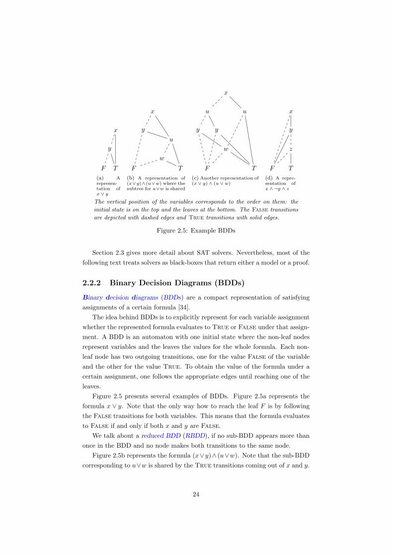
The vertical position of the variables corresponds to the order on them: the
initial state is on the top and the leaves at the bottom. The False transitions
are depicted with dashed edges and True transitions with solid edges.
Figure 2.5: Example BDDs
Section 2.3 gives more detail about SAT solvers. Nevertheless, most of the
following text treats solvers as black-boxes that return either a model or a proof.
2.2.2 Binary Decision Diagrams (BDDs)
Binary decision diagrams (BDDs) are a compact representation of satisfying
assignments of a certain formula [34].
The idea behind BDDs is to explicitly represent for each variable assignment
whether the represented formula evaluates to True or False under that assign-
ment. A BDD is an automaton with one initial state where the non-leaf nodes
represent variables and the leaves the values for the whole formula. Each non-
leaf node has two outgoing transitions, one for the value False of the variable
and the other for the value True. To obtain the value of the formula under a
certain assignment, one follows the appropriate edges until reaching one of the
leaves.
Figure 2.5 presents several examples of BDDs. Figure 2.5a represents the
formula x ∨ y. Note that the only way how to reach the leaf F is by following
the False transitions for both variables. This means that the formula evaluates
to False if and only if both x and y are False.
We talk about a reduced BDD (RBDD), if no sub-BDD appears more than
once in the BDD and no node makes both transitions to the same node.
Figure 2.5b represents the formula (x∨y)∧ (u∨w). Note that the sub-BDD
corresponding to u∨w is shared by the True transitions coming out of x and y.
24

The reason why that is possible is that once x∨y is True, whether the formula
is True or False depends solely on u and w.
We talk about an ordered BDD (OBDD) if there exist a linear order on the
variables such that no variable makes a transition to a variable that precedes it
in that order. As illustrated by the following example, the order may affect the
size of the BDD.
Figure 2.5c is another representation of (x∨y)∧(u∨w) where different order
of variables is used. Note that the size of this BDD is larger than the one in
Figure 2.5b. Intuitively, the reason for that is that the the values of y and w
are not independent of x and u.
In the BDD in Figure 2.5d the only way how to reach the leaf True is to
follow the True transition from x, False transition from y, and True transition
from z. This means that the BDD represents the formula x ∧ ¬y ∧ z.We talk about a ROBDD if a BDD is both reduced and ordered. Note
that all BDDs in Figure 2.5 are ROBDDs. Typically, the term BDD implicitly
implies ROBDD as most implementations enforce order and reduction.
2.3 Better Understanding of a SAT Solver
This section explains the basic principles of modern SAT solvers. Understanding
of this is necessary only for Section 4.4 and Section 6.3.1. This section greatly
simplifies the workings of a SAT solver and the interested reader is referred
to [138, 139, 158, 61].
Algorithms behind modern SAT solvers have evolved from the Davis-
Putnam-Longeman-Loveland procedure (DPLL) [50]. The basic idea of DPLL
is to search through the state space while performing constraint propagation
to reduce the space to be searched. Indeed, a SAT solver searches through
the space of possible variable assignments while performing unit propagation.
Whenever the assignment violates the given formula, the solver must backtrack.
The search terminates with success if all variables were assigned and the formula
is satisfied. The search terminates unsuccessfully if the whole search space was
covered and no satisfying assignment was found.
Before explaining the algorithm in greater detail, several terms are intro-
duced. The solver assigns values to variables until all variables have a value. A
value may be assigned either by propagation or by a decision.
Assignments made by propagation are necessitated by the previous assign-
ments. Decisions determine the part of the search space to be explored. Assign-
ments will be denoted by the corresponding literal, i.e., the assignment x means
that the variable x is assigned the value True, the assignment ¬x means that
the variable was assigned the value False.
25

A state of the solver consists of a partial assignment to the variables and the
decision level—the number of decisions on the backtracking stack. A unit clause
is a clause with all literals but one having the value False and the remaining
one without a value. A conflict is a clause whose all literals have the value
False.
Whenever a unit clause is found, the unassigned literal must have the value
True in order to satisfy that clause. Whenever a conflict is found, the current
variable assignment cannot satisfy the formula as all clauses must be satisfied.
The following example illustrates these terms.
Example 11. If the solver makes decisions x and y, the decision level is 2 and
the clause ¬x∨¬y∨z is a unit clause. While for the decisions x, y, ¬z the same
clause is a conflict.
Propagation consists of identifying unit clauses and assigning the value True
to the unassigned literal. Propagation terminates if a conflict is reached or there
are no unit clauses left.
Example 12. Let φdef= (¬x ∨ y) ∧ (¬x ∨ ¬y) and the decision made is x. Both
clauses are unit, if propagation picks the first one, it assigns to y the value True
and the second clause becomes a conflict. If, however, the solver makes the
decision y, the propagation assigns to x the value False as the second clause
is unit. Note that in this case there is no conflict and we have a satisfying
assignment for φ.
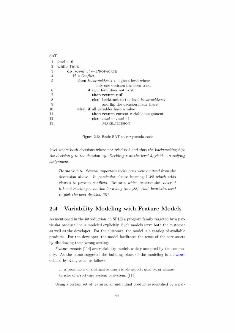
Figure 2.6 shows pseudo-code for a SAT solver based on the techniques out-
lined so far. The search alternates between propagation and making decisions.
Whenever the propagation detects a conflict, the search must backtrack, which
means flipping the decision for the highest level where only one decision has
been tried. This means, if the solver made the decision ¬v, it is flipped to v on
backtracking and vice-versa.
The SAT solver described above has an important property. That is once
the solver commits itself to a part of the search space, it finds a solution there
if one exists. This is captured by the following property.
Property 1. If the solver makes the decisions l1, . . . , ln and there exists a
solution to the given formula satisfying these decisions, the solver returns such
a solution.
Example 13. Let φdef= (¬x ∨ ¬y ∨ z) ∧ (¬x ∨ ¬y ∨ ¬z). The propagation does
not infer any new information and the solver makes the decision x. Again the
propagation does not do anything and the solver makes the decision y. Now, the
propagation infers a conflict and the solver must backtrack. The highest decision
26
SAT
1 level ← 02 while True3 do isConflict ← Propagate4 if isConflict5 then backtrackLevel ←highest level where
only one decision has been tried6 if such level does not exist7 then return null8 else backtrack to the level backtrackLevel9 and flip the decision made there
10 else if all variables have a value11 then return current variable assignment12 else level ← level +113 MakeDecision
Figure 2.6: Basic SAT solver pseudo-code
level where both decisions where not tried is 2 and thus the backtracking flips
the decision y to the decision ¬y. Deciding z at the level 3, yields a satisfying
assignment.
Remark 2.5. Several important techniques were omitted from the
discussion above. In particular clause learning [138] which adds
clauses to prevent conflicts. Restarts which restarts the solver if
it is not reaching a solution for a long time [83]. And, heuristics used
to pick the next decision [61].
2.4 Variability Modeling with Feature Models
As mentioned in the introduction, in SPLE a program family targeted by a par-
ticular product line is modeled explicitly. Such models serve both the customer
as well as the developer. For the customer, the model is a catalog of available
products. For the developer, the model facilitates the reuse of the core assets
by disallowing their wrong settings.
Feature models [114] are variability models widely accepted by the commu-
nity. As the name suggests, the building block of the modeling is a feature
defined by Kang et al. as follows.
... a prominent or distinctive user-visible aspect, quality, or charac-
teristic of a software system or system. [114]
Using a certain set of features, an individual product is identified by a par-
27
Root Feature
Mandatory Sub-feature
Optional Sub-feature
or-group
alternative-group
A B<<requires>>
A B<<excludes>>
Feature A requires B
Features A an B are mutually exclusive
(a) FODA modeling primitives
electric gas
engine
car
car-body
automatic manual
gearshiftpower-locks
<<excludes>>
key-less entry
<<requires>>
(b) Car feature tree
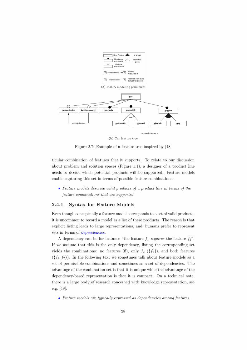
Figure 2.7: Example of a feature tree inspired by [48]
ticular combination of features that it supports. To relate to our discussion
about problem and solution spaces (Figure 1.1), a designer of a product line
needs to decide which potential products will be supported. Feature models
enable capturing this set in terms of possible feature combinations.
Feature models describe valid products of a product line in terms of the
feature combinations that are supported.
2.4.1 Syntax for Feature Models
Even though conceptually a feature model corresponds to a set of valid products,
it is uncommon to record a model as a list of these products. The reason is that
explicit listing leads to large representations, and, humans prefer to represent
sets in terms of dependencies.
A dependency can be for instance “the feature f1 requires the feature f2”.
If we assume that this is the only dependency, listing the corresponding set
yields the combinations: no features (∅), only f2 ({f2}), and both features
({f1, f2}). In the following text we sometimes talk about feature models as a
set of permissible combinations and sometimes as a set of dependencies. The
advantage of the combination-set is that it is unique while the advantage of the
dependency-based representation is that it is compact. On a technical note,
there is a large body of research concerned with knowledge representation, see
e.g. [49].
Feature models are typically expressed as dependencies among features.
28
2.4.2 FODA Notation
Kang et al. noticed that humans not only like to record sets of possibilities in
terms of dependencies but also like to organize things hierarchically. Kang et al.
introduced a user-friendly diagrammatic notation for recording features, com-
monly known as the FODA notation. As the notation is diagrammatic, it is
best explained in figures.
Figure 2.7a shows the modeling primitives of the notation. Figure 2.7b, is an
example of a feature tree representing possible configurations of a car. Each node
in the tree represents a feature, the children of a node are called sub-features
of the node. Some sub-features are grouped in order to express dependencies
between siblings. The node at the very top is called the root feature.
In this example, the diagram expresses that a car must have a body, a
gearshift, and an engine; an engine is electric or gas (selecting both corresponds
to a hybrid engine); a gearshift is either automatic or manual. Additionally, a
car may have power-locks or enable key-less entry. The two edges not part of
the hierarchy are called cross-cutting constraints. In this example they express
that a key-less entry cannot be realized without power-locks and the electric
engine cannot be used together with manual gearshift.
In general, this notation might not suffice to nicely express some dependen-
cies and then the designer can add dependencies in the form of an arbitrary logic
formula; such formulas are called left-over constraints or cross-tree constraints.
Remark 2.6. Technically, left-over constraints are not needed
as the FODA notation enables expressing any propositional for-
mula [179]. In practice, however, left-over constraints are indispens-
able when the designer of the model needs to capture a dependency
between features in different branches of the hierarchy. This is likely
to occur as the hierarchy is not so much driven by the propositional
semantics that the feature model is to capture but by the hierarchi-
cal organization of the features as seen in the real world by humans.
For instance, gear-shift is a sub-feature of a car because gear-shift is
a component of a car in the real world.
Feature trees suggest a nice way of selecting a particular feature-combination
(a product). The user selects or eliminates features starting from the root and
continues toward the leaves. The user must follow a simple set of rules in order
to stay within valid products. If the user has selected a feature, then he or she
must select a sub-feature if that is a mandatory feature; that is not required if
it is an optional sub-feature. If the user selects a feature then one and only one
sub-feature must be selected from an alternative-group1 and at least one must
1Sometimes alternative-groups are called xor-groups, which is misleading for groups with
29
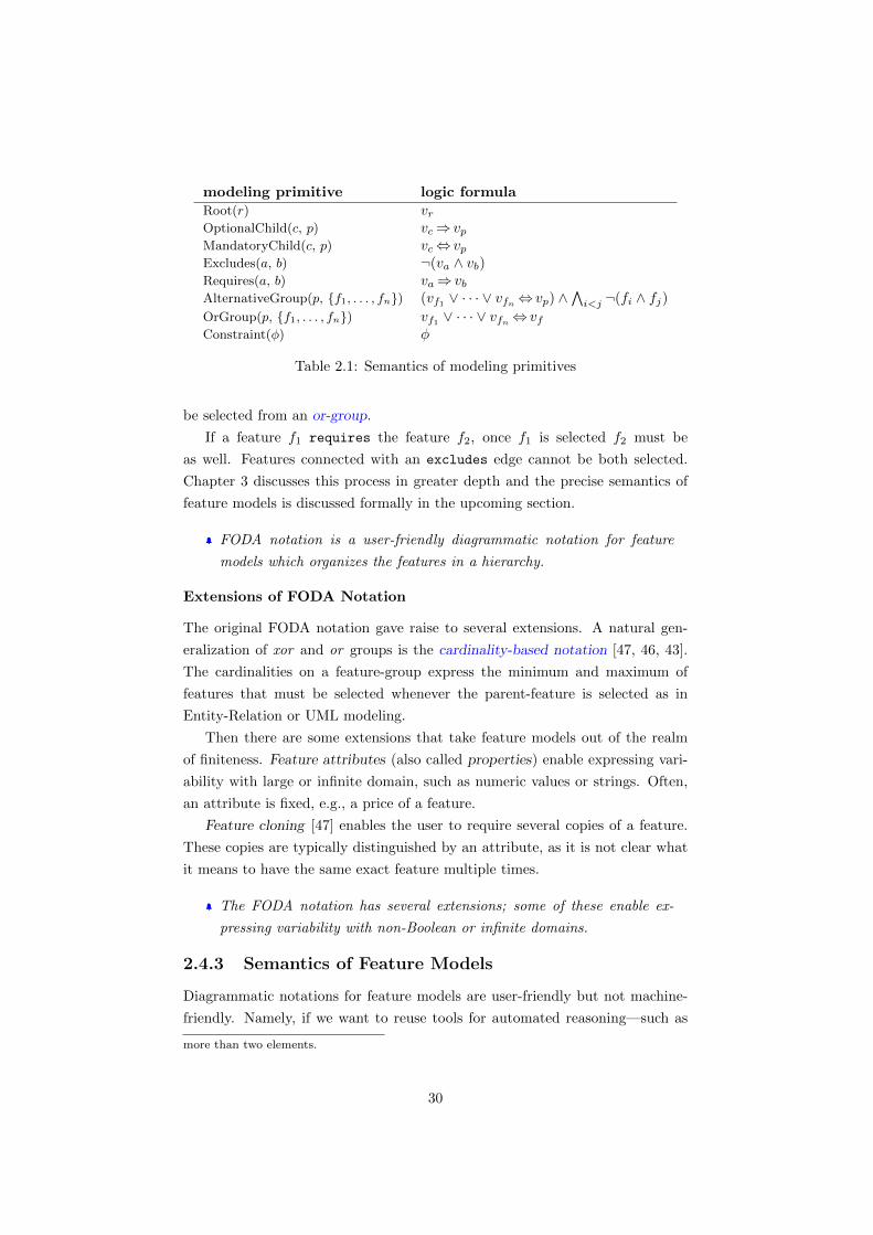
modeling primitive logic formulaRoot(r) vrOptionalChild(c, p) vc⇒ vpMandatoryChild(c, p) vc⇔ vpExcludes(a, b) ¬(va ∧ vb)Requires(a, b) va⇒ vbAlternativeGroup(p, {f1, . . . , fn}) (vf1 ∨ · · · ∨ vfn⇔ vp) ∧
∧i<j ¬(fi ∧ fj)
OrGroup(p, {f1, . . . , fn}) vf1 ∨ · · · ∨ vfn⇔ vfConstraint(φ) φ
Table 2.1: Semantics of modeling primitives
be selected from an or-group.
If a feature f1 requires the feature f2, once f1 is selected f2 must be
as well. Features connected with an excludes edge cannot be both selected.
Chapter 3 discusses this process in greater depth and the precise semantics of
feature models is discussed formally in the upcoming section.
FODA notation is a user-friendly diagrammatic notation for feature
models which organizes the features in a hierarchy.
Extensions of FODA Notation
The original FODA notation gave raise to several extensions. A natural gen-
eralization of xor and or groups is the cardinality-based notation [47, 46, 43].
The cardinalities on a feature-group express the minimum and maximum of
features that must be selected whenever the parent-feature is selected as in
Entity-Relation or UML modeling.
Then there are some extensions that take feature models out of the realm
of finiteness. Feature attributes (also called properties) enable expressing vari-
ability with large or infinite domain, such as numeric values or strings. Often,
an attribute is fixed, e.g., a price of a feature.
Feature cloning [47] enables the user to require several copies of a feature.
These copies are typically distinguished by an attribute, as it is not clear what
it means to have the same exact feature multiple times.
The FODA notation has several extensions; some of these enable ex-
pressing variability with non-Boolean or infinite domains.
2.4.3 Semantics of Feature Models
Diagrammatic notations for feature models are user-friendly but not machine-
friendly. Namely, if we want to reuse tools for automated reasoning—such as
more than two elements.
30

SAT solvers—we have to provide a semantics in terms of mathematical logic.
Additionally, a mathematical semantics increases the confidence that everybody
understands the syntax in the same way.
Propositional logic has proven to be a good candidate for FODA seman-
tics [179]. The semantics consists of a set of variables and a formula on these
variables. For each feature f , the variable vf is introduced representing whether
the pertaining feature is selected or not. The formula is constructed such that
there is a one-to-one correspondence between satisfying assignments of the for-
mula and the permissible feature combinations of the feature model.
Table 2.1 presents the semantics of the individual modeling primitives of
the FODA notation; the semantics of a feature model is a conjunction of the
individual semantics. Note that there is always an implication from a sub-feature
to its parent, i.e., a sub-feature cannot be selected without its parent.
x
y
a b c d
⇔⇐ ⇐
xor
(a) Feature model example
vx ∧vy⇔ vx ∧vc⇒ vx ∧ vd⇒ vx ∧va⇒ vy ∧ vb⇒ vy ∧vy⇒(va ∨ vb) ∧vy⇒¬(va ∧ vb)
(b) Its semantics
Figure 2.8: FODA notation and its semantics
Figure 2.8 illustrates the semantics on a concrete toy-example. The left-hand
side of the figure is a small feature tree in the FODA notation2. The right-hand
side captures its semantics in term of a propositional formula obtained by using
the rules from Table 2.1.
Semantics of Extensions of FODA
As most of this thesis is dealing with the actual logic semantics of feature models
rather than the syntax, we are not going into great detail of semantics of FODA
extensions and the reader is referred to relevant publications. Propositional
logic semantics have been extensively studied by Schobbens et al. [179].
Jonge and Visser [51] propose the use of context-free grammars for capturing
the semantics of feature models. Feature configurations conforming to a feature
model are defined as the sentences generated by the pertaining grammar. This
idea is extended by Batory [15] by combining grammars and propositional logic.
Czarnecki et al. [47] also use context-free grammars to capture the semantics
of feature models. Their meta-model is more expressive than the feature models
2The labels on the edges are not part of the notation and are meant to represent thesemantics.
31
covered by the aforementioned articles, as their meta-model enables cardinalities
and feature cloning. The main limitation of grammars is that they do not enable
cross-tree dependencies.
Hofner et al. take an algebraic approach to feature modeling. In this ap-
proach, a product family is a set of sets of features, and the language of algebra
is used to abstract from the sets. Dependencies, such as exclusion, are expressed
as additional equalities. What makes this approach interesting is that it enables
to use multisets (sets with repetitions of an element, also known as bags) instead
of sets. This extension permits the modeling of feature models with cloning.
Even though this approach seems interesting, no other publications along this
line of research are known [97].
Benavides et al. user Constraint Satisfaction Problems to capture semantics
of feature models with attributes [21].
The author of this dissertation developed an approach to formalizing fea-
ture models in higher-order logic using the proof assistant PVS. Thanks to the
expressive power of the PVS language and higher order logic, this approach
enables reasoning about the full range of feature models—with cloning or at-
tributes [101].
32
Chapter 3
Configuring Variability
Models
We established that variability models represent a set of configurations that a
particular product line is set out to be able to implement. If users are config-
uring such model, they are looking for a particular configuration that respects
the model and also fulfills their requirements. In this chapter we establish a
connection between configuration and propositional logic.
In the case of feature models, the set of configurations is not recorded as a
catalog of configurations but as a set of constraints imposed on these configura-
tions since constraints enable more compact representation. However, it is hard
for a user to keep track of all the constraints for large and complex systems.
Hence, it is practical for the users to specify their requirements on the desired
configuration in a series of steps and reflect on the result of each step.
Section 2.4.1 suggests that for the FODA notation it is intuitive to start
making decisions about features from the root towards the leaves. In the follow-
ing, however, we do not assume any particular order of selecting or eliminating
features as that would be an unnecessary assumption about the user.
In fact, in general there is little that we assume about the decisions that users
might make. We do assume, however, that they wish to respect the constraints
of the product line specified by the feature model. This assumption is justified
by the fact that breaking the constraints given by the feature model would likely
require a change in the whole product line and thus incur higher development
cost, or, it might be the case that the constraint represents an actual physical
impossibility.
Conceptually, the configuration process can be thought of as a series of sets of
configurations (see Figure 3.1). The first set comprises the set of configurations
33
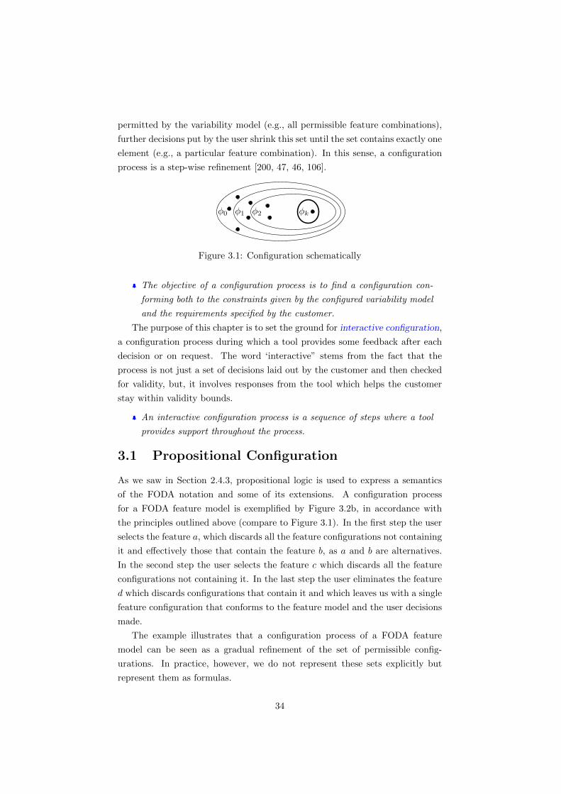
permitted by the variability model (e.g., all permissible feature combinations),
further decisions put by the user shrink this set until the set contains exactly one
element (e.g., a particular feature combination). In this sense, a configuration
process is a step-wise refinement [200, 47, 46, 106].
φ0 φ2φ1 φk
Figure 3.1: Configuration schematically
The objective of a configuration process is to find a configuration con-
forming both to the constraints given by the configured variability model
and the requirements specified by the customer.
The purpose of this chapter is to set the ground for interactive configuration,
a configuration process during which a tool provides some feedback after each
decision or on request. The word ‘interactive” stems from the fact that the
process is not just a set of decisions laid out by the customer and then checked
for validity, but, it involves responses from the tool which helps the customer
stay within validity bounds.
An interactive configuration process is a sequence of steps where a tool
provides support throughout the process.
3.1 Propositional Configuration
As we saw in Section 2.4.3, propositional logic is used to express a semantics
of the FODA notation and some of its extensions. A configuration process
for a FODA feature model is exemplified by Figure 3.2b, in accordance with
the principles outlined above (compare to Figure 3.1). In the first step the user
selects the feature a, which discards all the feature configurations not containing
it and effectively those that contain the feature b, as a and b are alternatives.
In the second step the user selects the feature c which discards all the feature
configurations not containing it. In the last step the user eliminates the feature
d which discards configurations that contain it and which leaves us with a single
feature configuration that conforms to the feature model and the user decisions
made.
The example illustrates that a configuration process of a FODA feature
model can be seen as a gradual refinement of the set of permissible config-
urations. In practice, however, we do not represent these sets explicitly but
represent them as formulas.
34
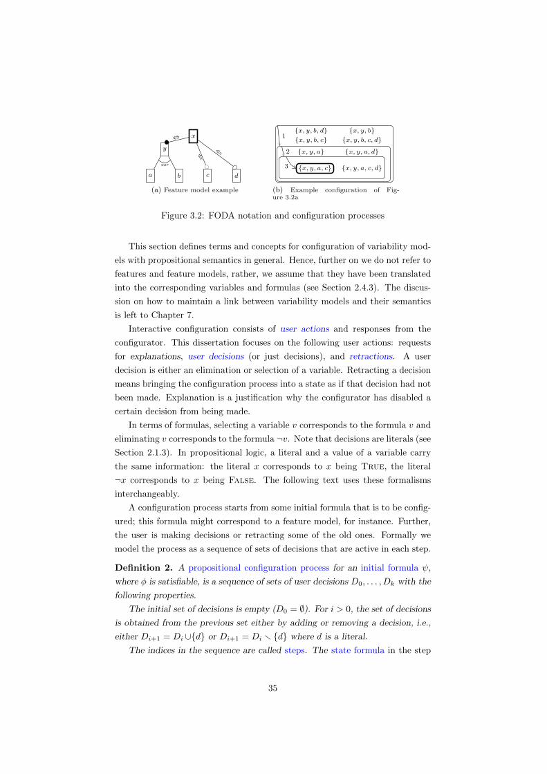
x
y
a b c d
⇔
⇐ ⇐
xor
(a) Feature model example
{x, y, a, c}
1
2
3
{x, y, b}{x, y, b, d}{x, y, b, c, d}{x, y, b, c}
{x, y, a} {x, y, a, d}
{x, y, a, c, d}
(b) Example configuration of Fig-ure 3.2a
Figure 3.2: FODA notation and configuration processes
This section defines terms and concepts for configuration of variability mod-
els with propositional semantics in general. Hence, further on we do not refer to
features and feature models, rather, we assume that they have been translated
into the corresponding variables and formulas (see Section 2.4.3). The discus-
sion on how to maintain a link between variability models and their semantics
is left to Chapter 7.
Interactive configuration consists of user actions and responses from the
configurator. This dissertation focuses on the following user actions: requests
for explanations, user decisions (or just decisions), and retractions. A user
decision is either an elimination or selection of a variable. Retracting a decision
means bringing the configuration process into a state as if that decision had not
been made. Explanation is a justification why the configurator has disabled a
certain decision from being made.
In terms of formulas, selecting a variable v corresponds to the formula v and
eliminating v corresponds to the formula ¬v. Note that decisions are literals (see
Section 2.1.3). In propositional logic, a literal and a value of a variable carry
the same information: the literal x corresponds to x being True, the literal
¬x corresponds to x being False. The following text uses these formalisms
interchangeably.
A configuration process starts from some initial formula that is to be config-
ured; this formula might correspond to a feature model, for instance. Further,
the user is making decisions or retracting some of the old ones. Formally we
model the process as a sequence of sets of decisions that are active in each step.
Definition 2. A propositional configuration process for an initial formula ψ,
where φ is satisfiable, is a sequence of sets of user decisions D0, . . . , Dk with the
following properties.
The initial set of decisions is empty (D0 = ∅). For i > 0, the set of decisions
is obtained from the previous set either by adding or removing a decision, i.e.,
either Di+1 = Di ∪{d} or Di+1 = Di r {d} where d is a literal.
The indices in the sequence are called steps. The state formula in the step
35

i ∈ 0 . . . k is the formula ψ0 ∧∧d∈Di
d.
Recall that the goal of a configuration process is to find a particular solution
of the initial formula. Hence, we consider a configuration process to be complete
if it determines one particular solution. In the context of propositional logic,
solutions correspond to satisfying variable assignments (models of the formula).
These concepts are captured in the following definition.
Definition 3. We say that a configuration process is complete iff the state
formula in the last step has one and only one satisfying assignment.
A configurator is a tool that assists the user during a configuration process.
The main role of a configurator is to prevent the user from making “wrong” de-
cisions. Informally, a decision is wrong if the configuration cannot be completed
without changing this decision. On the other hand, it should not prevent the
user from finding permissible solutions. The following definition captures these
two requirements.
Definition 4. We say that a configurator is backtrack-free iff does not allow
configuration processes with unsatisfiable state formulas.
A configurator is complete iff for any satisfying assignment of the initial
formula there exists a complete process where the state formula in the last step
is satisfied by this assignment.
Remark 3.7. There does not seem to be any motivation on behalf
of the user for a configurator to be not complete. If a configurator
is not complete, it means that the designer of the instance being
configured included some possibilities that the user cannot reach.
However, Freuder shows that the problem of backtrack-free interac-
tive configuration can become computationally easier if completeness
is sacrificed [77].
In some approaches, the user is enabled to temporally choose
non-backtrack-free options. This might happen if some external
conditions change or if there are multiple users on figuring the
same instance. In these cases interactive reconfiguration or correc-
tive explanations can be used to get back within the overall con-
straints [91, 159, 199]. However, the configurator needs to be aware
of the fact that backtrack-freeness was violated in order to invoke
such mechanism.
In the remainder of this section we make several observations about the
properties of the definitions above. These properties are closely tied to the
concept of bound variables and literals, which are defined as follows.
36

Definition 5. We say that a variable v is bound to the value True in a formula
φ iff it has the value True in all satisfying assignments of φ. Analogously, we
say that a variable v is bound to the value False in a formula φ iff it has
the value False in all satisfying assignments of φ. We say that a variable v is
bound if it is bound to some value. In a mathematical notation, for v bound to
True it holds φ |= v and it holds φ |= ¬v for v bound to False.
We extend the terminology for literals as well, we say that a literal l is bound
in φ iff it evaluates to True in all satisfying assignments of φ, i.e., it holds φ |= l.
Note that a variable v is bound in a formula iff one of the literals v, ¬v is
bound in the formula. If both of these literals are bound, the formula is unsatis-
fiable. To determine whether a literal is bound, it is possible to ask the question
whether the complementary literal can ever be satisfied; this is formalized by
the following proposition. (Recall that l denotes the literal complementary to
the literal l, Section 2.1.3.)
Proposition 1. A literal l is bound in ψ iff the formula ψ ∧ l is unsatisfiable.
Proof. First we observe that ψ ∧ l has those satisfying assignments that satisfy
both ψ and l. Additionally, for any assignment either l or l holds (but not both).
If ψ |= l, then all satisfying assignments of ψ satisfy l and therefore there
are no assignments satisfying l. If there are no satisfying assignments of ψ ∧ l,then l must be satisfied by all satisfying assignments of ψ.
The following observation relates bound variables and complete processes.
Observation 1. A configuration process is complete iff all variables are bound
in the state formula of the last step.
Example 14. Let φi denote state formulas of a process starting from φ0def=
(¬u ∨ ¬v) ∧ (x⇒ y). The user selects u (φ1def= φ0 ∧ u); v is bound to False
as u and v are mutually exclusive. The user sets y to False (φ2def= φ1 ∧ ¬y);
the variable x is bound to False. The process is complete as all variables are
bound.
The following propositions show that a backtrack-free and complete con-
figurator enforces decisions that are bound. Conversely, it disallows decisions
whose complement is bound. This observation is used in Chapter 4 to construct
a configurator.
Proposition 2. A configurator is backtrack-free iff it does not permit decisions
d such that d is bound in the current state formula.
Proof. In the following, φi and φi+1 denote two consequent state formulas. First,
if a configurator is backtrack-free, then it must not allow to make a decision d if
37

d is bound. Since if it did allow such decision, it holds φi |= d and φi+1 ≡ φi ∧dwhere φi+1 is unsatisfiable due to Proposition 1.
Now we show, by contradiction, that if it does not allow to make decisions
d whose complement is not bound, then the configurator is backtrack-free. Let
us assume that the configurator is not backtrack-free and therefore there exists
an unsatisfiable state formula φi in some process. Since the initial formula is
satisfiable by definition, the first state formula cannot be the unsatisfiable one. If
a state formula φi ≡ φi−1∧ l is unsatisfiable, then φi−1 |= l due to Proposition 1
and that is a contradiction because the decision l is not allowed.
Proposition 3 (Completeness). If a configurator allows any decision whose
complement is not bound, then it is complete.
Proof. Let l0, . . . , ln be literals representing a satisfying assignment of φ0, in
some (arbitrary) order. Since φ0 ∧ l0 ∧ · · · ∧ li ∧ li+1 is satisfiable for any
i ∈ 0..n− 1, the literal li+1 is not bound due to Proposition 1. Hence, the
configurator allows the decision li+1 in the step i. The desired assignment is
obtained by the decisions l0, . . . , ln in this order.
3.2 Summary
A configuration process can be seen as a gradual refinement of the set of config-
urations. In SPLE we represent the set of configurations using feature models.
Feature models captured in the FODA notation have semantics expressible in
propositional logic. We translate the given feature model into its semantics and
similarly represent user decisions as logic formulas. Conjoining the semantics of
a feature model with user decisions gives us the state formula (Definition 2).
A configurator is a tool that provides a user with feedback throughout the
configuration process (hence making the process interactive). A configurator is
backtrack-free iff it does not allow such sequences of user decisions that cannot
be extended into a valid configuration. A configurator is complete iff it allows
all sequences of user decisions that lead into a valid configuration (Definition 4).
We define the term bound literal (Definition 5) as a literal that is true in all
valid configurations, and, we show that whether a literal is bound or not, can
be phrased as a satisfiability question (Proposition 1). Finally, we show that a
completeness and backtrack-freeness of a configurator is achieved by identifying
bound literals throughout the process. This is particularly important in the
following chapter as it makes a connection between backtrack-free and complete
configurators, and, satisfiability.
38

Chapter 4
Interactive Configuration
with a SAT Solver
This chapter describes how to use a SAT solver to implement a complete and
backtrack-free configurator. The implementation relies on propositions 2 and 3
which tell us that completeness and backtrack-freeness is achieved by identifying
bound literals.
The presentation is carried out in the following steps. Section 4.1 describes
the context in which the algorithms operate. Section 4.2 presents the main
ideas of an algorithm for finding bound literals and a naive version of this
algorithm. This naive version is improved in Section 4.3; this improvement
has the property of being easy to implement while it significantly improves
the performance. Section 4.5 focuses on an aspect neglected by the previous
sections—the explanations for the feedback given to the user by the configurator.
4.1 Setup
All the presented algorithms expect the initial formula to be given in the con-
junctive normal form (CNF); how the CNF is obtained is discussed in Chapter 7.
The presentation of the algorithms is done in the context depicted in Figure 4.1.
The centerpiece is the configurator which communicates with two components:
the user interface and a SAT solver.
The communication is carried out through a set of messages. The user
interface initializes the configurator with an initial CNF formula by sending the
message Init(ψ : CNF ); all the inference from then on assumes that this formula
holds and therefore the message requires that the formula is satisfiable. The user
interface communicates a new user decision by the message Assert(l : Literal).
39

User Interface Configuration SAT Solving
Init(φ)
Assert(l)
Retract(l)
Explain(x)
Lock(x, v)
Unlock(x)
IsSAT(ψ)
Refute(ψ)
Figure 4.1: Configuration process
The user interface requests to retract a previously made decision by sending
Retract(l : Literal). Asserting a previously asserted literal without retracting
it has no effect. Analogously, retracting a literal not asserted has no effect.
Asserting the literal v corresponds to selecting the variable v and asserting
the literal ¬v corresponds to eliminating the variable. The user interface may
send Assert and Retract messages only with literals that contain a variable
that appears in the initial formula ψ sent in the initialization message. More
specifically, this means that the set of variables whose values are to be configured
remains the same throughout the configuration process.
Remark 4.8. The actual implementation enables configuring vari-
ables not appearing in ψ0 by letting the user interface specify explic-
itly the set of variables that should be considered. However, these
variables are trivially unbound independently of the other variables
and can become bound only if the user interface sends the corre-
sponding Assert message.
The configurator uses the message Lock(x : Variable, v : Boolean) to lock
a variable in a certain value and it uses Unlock(x : Variable) to unlock a
variable. Note that the pair (x : Variable, v : Boolean) passed to the message
Lock corresponds to a literal: if v is True, the corresponding literal is x; if v
is False, the corresponding literal is ¬x.
The user interface guarantees that it does not send Assert messages
concerning a locked variable. In other words, the user interface pre-
vents its users from changing values of locked variables. The message
Lock(x : Variable, v : Boolean) is sent when the variable x is bound to the
value v.
Note that the mechanism of locking ensures completeness and backtrack-
freeness of the configurator due to propositions 3 and 2. If one of the literals
v, ¬v is bound, the configurator locks the variable v and therefore the user can
never make a decision whose complement is bound.
40
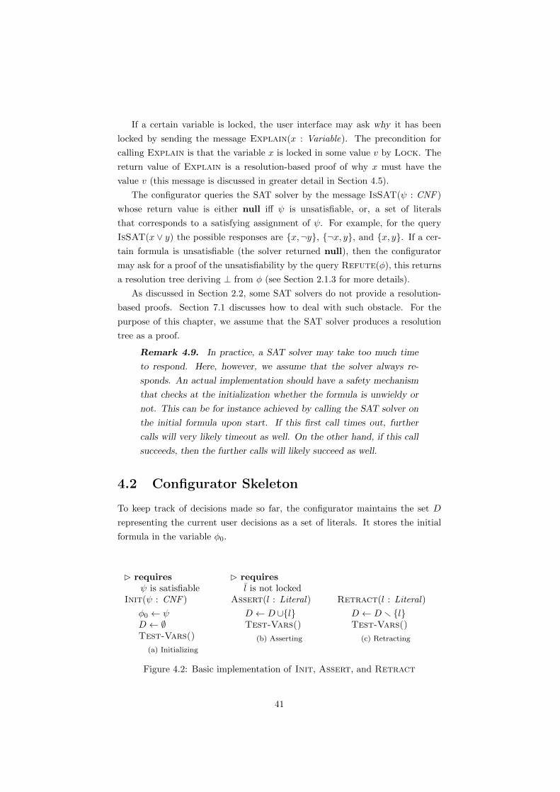
If a certain variable is locked, the user interface may ask why it has been
locked by sending the message Explain(x : Variable). The precondition for
calling Explain is that the variable x is locked in some value v by Lock. The
return value of Explain is a resolution-based proof of why x must have the
value v (this message is discussed in greater detail in Section 4.5).
The configurator queries the SAT solver by the message IsSAT(ψ : CNF )
whose return value is either null iff ψ is unsatisfiable, or, a set of literals
that corresponds to a satisfying assignment of ψ. For example, for the query
IsSAT(x ∨ y) the possible responses are {x,¬y}, {¬x, y}, and {x, y}. If a cer-
tain formula is unsatisfiable (the solver returned null), then the configurator
may ask for a proof of the unsatisfiability by the query Refute(φ), this returns
a resolution tree deriving ⊥ from φ (see Section 2.1.3 for more details).
As discussed in Section 2.2, some SAT solvers do not provide a resolution-
based proofs. Section 7.1 discusses how to deal with such obstacle. For the
purpose of this chapter, we assume that the SAT solver produces a resolution
tree as a proof.
Remark 4.9. In practice, a SAT solver may take too much time
to respond. Here, however, we assume that the solver always re-
sponds. An actual implementation should have a safety mechanism
that checks at the initialization whether the formula is unwieldy or
not. This can be for instance achieved by calling the SAT solver on
the initial formula upon start. If this first call times out, further
calls will very likely timeout as well. On the other hand, if this call
succeeds, then the further calls will likely succeed as well.
4.2 Configurator Skeleton
To keep track of decisions made so far, the configurator maintains the set D
representing the current user decisions as a set of literals. It stores the initial
formula in the variable φ0.
� requiresψ is satisfiable
Init(ψ : CNF )
φ0 ← ψD ← ∅Test-Vars()
(a) Initializing
� requiresl is not locked
Assert(l : Literal)
D ← D∪{l}Test-Vars()
(b) Asserting
Retract(l : Literal)
D ← D r {l}Test-Vars()
(c) Retracting
Figure 4.2: Basic implementation of Init, Assert, and Retract
41

Test-Vars()
1 φ← φ0 ∧∧l∈D l
2 foreach x : vars-of(φ0)3 do CanBeTrue ← TEST-SAT(φ, x)4 CanBeFalse ← TEST-SAT(φ,¬x)5 if ¬CanBeTrue ∧¬CanBeFalse6 then error “Unsatisfiable”7 if ¬CanBeTrue then Lock(x, False)8 if ¬CanBeFalse then Lock(x, True)9 if CanBeTrue ∧CanBeFalse then Unlock(x)
Figure 4.3: Skeleton of the algorithm for testing bound variables
Figure 4.2 shows an implementation of the procedures Init, Assert, and
Retract. All of these procedures rely on the procedure Test-Vars, whose job
is to analyze the newly established state and compute the appropriate binding
for the variables.
Figure 4.3 presents a pseudo-code for Test-Vars which computes, for each
literal, if it is bound in the current state formula. To do that, it relies on
Proposition 1, which tells us that a literal l is bound in the formula φ iff φ ∧ lis unsatisfiable. In order to test this, the procedure Test-Vars uses a function
Test-SAT(ψ : CNF , l : literal), which tests the satisfiability of ψ ∧ l and is
discussed later on.
The two calls to Test-SAT have four possible outcomes and these are in-
vestigated in the lines 5–9. If the variable x can be neither True nor False,
then φ itself is unsatisfiable (line 5), which breaks the assumptions that φ is sat-
isfiable at all times as the configurator is backtrack-free (this possibility occurs
only when some of the contracts of the procedures are broken). If the variable
can be either True or False, but not both, then the variable is locked in the
complementary value (lines 7 and 8). If the variable can be both True and
False, the algorithm makes sure that the variable is unlocked (line 9).
Test-SAT(ψ: Formula, l: Literal) : Boolean
return IsSAT(ψ ∧ l) 6= null
Figure 4.4: Naive version of Test-SAT
Now, let us look at the implementation of Test-SAT. Since the algorithm
has a SAT solver at its disposal, it can simply query the solver for the satisfiabil-
ity of φ∧ l as shown in Figure 4.4. This yields an algorithm that calls the solver
42

twice on each variable after each assertion and retraction. (Test-SAT always
invokes the solver and Test-Vars invokes Test-SAT twice for each variable.)
Remark 4.10. Note that the order of iterating through the set of
variables in Test-Vars does not influence which variables will be
locked and which not. The reason for that is that whether a variable
v is locked or not solely depends on the satisfiability of φ ∧ v and
φ ∧ ¬v and the formula φ does not change during the iteration.
4.3 Computation Reuse
As pointed out, the version of Test-SAT above calls the SAT solver consid-
erably many times—twice for each variable after each user action. This is im-
proved if we realize that the iterations of the loop in Test-Vars do not in any
way reuse information gained in the previous iterations. Let us look how that
can be done.
First, consider the situation when the algorithm tests the satisfiability of
φ ∧ l and the solver returns a satisfying assignment. If that assignment gives the
value True to some variable x, then φ ∧ x must be satisfiable as this assignment
is a witness for the fact that φ ∧ l ∧ x is satisfiable. Therefore, there is no need
to call the solver on φ ∧ x after that. Analogously, if the assignment gives False
to x, then φ∧¬x is satisfiable and there is no need to call the solver on φ ∧ ¬x.
Example 15. Let ψdef= x ∨ y ∨ z and assume that IsSAT(ψ ∧ x) responds
{x, y,¬z}. From the response of the solver we know that ψ∧x is satisfiable but
also that ψ ∧ y and ψ ∧ ¬z are satisfiable.
Based on this observation, the first improvement to the algorithm is to avoid
satisfiability tests of values that appear in some of the satisfying assignments
encountered so far. This optimization does not exploit, however, the negative re-
sponses of the solver (null). Consider the situation when the constraint contains
the formula ¬x1 ∨ x2. If the solver knows that x2 must be False, it can quickly
deduce that x1 must be False by using unit propagation (see Section 2.1). In
general, conjoining the bound literal gives to the solver more information about
the formula and the solver is expected to perform better. This motivates the
second improvement: storing the values that are disallowed and conjoining their
complements to the whole formula in subsequent queries. We refer to this op-
timization as catalyst optimization as the literals being conjoined should speed
43

up the solving process (serve as catalysts).
Remark 4.11. The optimization just introduced is analogous to the
way lemmas are used in mathematical proofs. If φ∧ l is unsatisfiable,
then φ |= l and this knowledge is used in further inference just as
lemmas are used to prove other theorems.
Based on these two ideas, we devise a new version of Test-SAT. This version
is again called from Test-Vars (see Figure 4.3).
Test-SAT(ψ: CNF , l: Literal) : Boolean
1 if l ∈ KnownValues then return True2 if l ∈ DisabledValues then return False3 L← IsSAT(ψ ∧ l ∧
∧k∈DisabledValues k)
4 if L 6= null5 then KnownValues ← KnownValues ∪L6 else DisabledValues ← DisabledValues ∪{l}7 return L 6= null
Figure 4.5: Improved Test-SAT
This new version (see Figure 4.5) relies on two sets DisabledValues and
KnownValues. The set DisabledValues comprises literals l for which the algo-
rithm knows that φ∧ l is unsatisfiable, and the set KnownValues comprises the
literals l for which the algorithm knows that φ ∧ l is satisfiable for the current
state formula φ. For instance, if DisabledValues contains the literal ¬x, then
x must not be False in the current state formula—it is bound to True; if
KnownValues contains the literal ¬y, then y can be True in the current state
formula so it is certainly not bound to False.
How the sets DisabledValues and KnownValues are updated between differ-
ent calls to Test-Vars is discussed after the description of Test-SAT—recall
that Test-SAT is invoked from Test-Vars on the current state formula.
Test-SAT first consults the two sets and does not invoke the solver if the
queried literal is in any of them (lines 1 and 2). If it does call the solver and
ψ ∧ l is satisfiable, it adds into KnownValues all the literals that are in the
returned satisfying assignment (line 7). If ψ ∧ l is unsatisfiable, then it adds the
literal l into the set DisabledValues (line 8).
Note that if a variable x is not bound to any value, then eventually both
literals x and ¬x will be in the set KnownValues. In contrast, the literals x and
¬x will never both end up in the set DisabledValues as that would mean that x
can be neither True nor False. Hence, if a literal l is in DisabledValues, then
the literal l will end up in KnownValues as the literal l is bound in the current
44

Init(ψ : CNF )
φ← ψD ← ∅KnownValues ← ∅DisabledValues ← ∅Test-Vars()
Assert(l : Literal)
D ← D∪{l}KnownValues ← ∅Test-Vars()
Retract(l : Literal)
D ← D r {l}DisabledValues ← ∅Test-Vars()
Figure 4.6: Change of state and KnownValues and DisabledValues.
state formula.
Observation 2. If ψ ∧ l is satisfiable, then the literal l itself must be among
the returned literals. Therefore Test-SAT never invokes the solver twice on
the same query.
So far it has not been specified how to initialize the sets KnownValues and
DisabledValues neither it was said how asserting and retracting affects them.
A rather coarse approach would be to empty both sets whenever φ changes,
i.e., in Init, Assert, and Retract. However, any assertion strengthens φ
and therefore it is safe to keep DisabledValues. Conversely, decision retracting
weakens φ and it is safe to keep KnownValues. This is captured by the two
following observations.
Observation 3. After a retraction, the literals in the set KnownValues are still
possible assertions for the new state-formula.
Proof. Let φ ≡ φ′ ∧ l be the state-formula before the retraction and φ′ be the
state-formula after retraction. The formula φ′ “constrains less” (it is weaker).
In other words, all the satisfying assignments of φ are also satisfying assignments
of φ′. Hence, if φ′ ∧ l ∧ k is satisfiable for some literal k ∈ KnownValues, then
φ′ ∧ k is also satisfiable.
Observation 4. After an assertion, the literals in the set DisabledValues are
still impossible to be asserted for the new state-formula.
Proof. Let φ be the state-formula before the assertion and φ′ ≡ φ ∧ l the state-
formula after the assertion. The formula φ′ “constrains more” (it is stronger).
Hence, if φ∧k is unsatisfiable for some literal k ∈ DisabledValues, then φ∧ l∧kmust be unsatisfiable as well.
4.3.1 Example Execution
The following text describes a sample configuration process using the described
algorithm. The notation φi is used to represent the state formula in step i. The
45

user interface initializes the process with the formula to be configured defined
as follows.
ψ0def= p⇒(q⇒ r) ∧
p⇒(¬q ∨ ¬r)
Initialization The procedure Init stores the initializing formula ψ into φ0
and sets each of the D, DisabledValues, and KnownValues to the empty set and
calls Test-Vars.
Initial Test The procedure Test-Vars begins by testing the variable p. Since
φ0∧p is satisfiable, the SAT solver finds a satisfying assignment {p,¬q, r}, whose
literals are added to KnownValues. Similarly, the query φ0∧¬p yields the literals
{¬p, q,¬r}, which also are added to KnownValues.
Thanks to the luck we had in finding satisfying assignments, the tests for
the variables r and q do not need to use the SAT solver since all four pertaining
literals are already in KnownValues.
Assert Now the user makes the decision that the variable p should be True,
this yields the invocation Assert(p). Assert adds the literal p to the set D
and clears the set KnownValues. This gives us the state formula φ1def= φ0 ∧ p.
For better intuition, the formula φ1 can be rewritten as follows.
φ1def= (q⇒ r) ∧
(¬q ∨ ¬r)
Test after decision The procedure Assert invokes Test-Vars. The SAT
solver responds {p, r,¬q} and {p,¬r,¬q} to the queries φ1 ∧ r and φ1 ∧ ¬r,respectively. Hence, both True and False are possible for the variable r, while
for q we only know that it can be False under this state formula.
The SAT solver tells us that φ1 ∧ q is unsatisfiable and the algorithm locks
the variable q in the value False. The configuration process is complete as all
variables are bound.
Remark 4.12. Even this small example shows that unit prop-
agation (see Section 2.1.3) is an insufficient inference mechanism
for configuration (as in [15]). Applying unit propagation to p ∧(p⇒(q⇒ r)) ∧ (p⇒(¬q ∨ ¬r)) yields p ∧ (q⇒ r) ∧ (¬q ∨ ¬r), from
which it is not obvious that q must be False.
46

4.3.2 Discussion about Complexity
This section makes several observations regarding the computational complexity
of the approach. A first thing that should be justified is the use of a SAT solver.
Satisfiability in general is an NP-complete problem. Couldn’t determining the
satisfiability of φ ∧ l be easier? The following claim shows that it is just as
difficult.
Claim 1. Let φ be a CNF formula and let l be a literal. Then the satisfiability
of φ ∧ l (which is also CNF) is NP-complete.
Proof. Let ψ be a formula and x a variable not appearing in ψ. Let ψ′ be a
CNF of the formula x⇒ψ. The formula ψ′ is obtained from ψ by adding the
literal ¬x to each clause (hence, the size of ψ′ is linear in the size of ψ). Since
ψ′ ∧ x and ψ are equisatisfiable, answering the query of satisfiability of ψ′ ∧ xanswers satisfiability of ψ, which means solving an NP-complete problem and
thus the satisfiability of φ ∧ l is NP-hard. The satisfiability of φ ∧ l is in NP
because it can be checked in polynomial time that an assignment satisfies the
formula φ ∧ l, i.e., the problem is NP-complete.
Claim 2. To determine whether a literal l is bound in a formula φ is co-NP
complete.
Proof. An immediate consequence of previous claim and Proposition 1.
As the above claims show, the procedure Test-Vars (Figure 4.3) solves
two NP-complete problems for each variable: the satisfiability of φ ∧ x and the
satisfiability of φ∧¬x. As the SAT solver is the place where this happens, it is
interesting to look at how many times the solver is called in that procedure.
Claim 3. If n is the number of variables of the problem being configured, then
the SAT solver is called no more than n+ 1 times.
Proof. For each variable y there are the two complementary literals y and
¬y. Therefore there are 2n different literals whose satisfiability the procedure
Test-Vars must answer.
Let x be the first variable being tested in Test-Vars. At least one of the two
calls to the solver for satisfiability of φ ∧ x and φ ∧ ¬x must return a satisfying
assignment otherwise φ would be unsatisfiable. Therefore, after the first test of
the first variable, the set KnownValues contains at least n − 1 literals that do
not contain the variable x. In other words, we know that at least one of the
literals corresponding to any of the variables succeeding x is satisfiable.
47

Remark 4.13. Here I would like to make a highly intuitive remark
concerning the case when the solver is called many times (close to
n + 1). One scenario when the SAT solver is called n + 1 times is
when there is exactly one satisfying assignment of the formula. In
that case the solver will respond negatively for all the literals that
have not been tested yet after the test of the first variable. If that is
the case, then it is likely that the variables are strongly constrained
and the solver will return quickly from these queries.
Another extremal case is when the solver returns satisfying assign-
ments but the set KnownValues is being filled slowly, which means
that the different satisfying assignments returned by the solver are
very similar even though the queries are different. In such case the
dependencies between variables must be loose and again, the solver
is likely to find the solution quickly. In summary, these two intuitive
observations suggest that if the solver is called many times, then the
individual calls will be fast.
The number of calls to the SAT solver decreases if testing satisfiability
of a variable reuses information obtained from previous tests.
4.4 Modifying the Solver
Kuchlin and Kaiser study how to compute the set of bound variables using a
SAT solver in a non-interactive setting [113]. Their algorithm is based on similar
principles as the algorithm Test-Vars, however, the state of the configuration
process is not maintained. The optimization they use is based on modifying
how the solver looks for solutions. This section shows how to implement this
optimization in our setting.
Recall that the set KnownValues stores the literals that have occurred in the
satisfying assignments found in the previous iterations of the loop in the function
Test-Vars. And, if a literal is already in this set, it is not necessary to test if
it is satisfiable in the current state formula because we know that it is. Hence,
it is desirable to maximize the number of literals in the satisfying assignments
that are not in the set KnownValues, in order to speed up its growth.
Example 16. Let the state formula be equivalent to True, then it is possible
to determine all the bound variables in two calls to the solver. In the first
call the solver returns all negative literals and in the second call it returns all
positive literals. Hence, the procedure Test-SAT never calls the solver again
since all the literals are in the set KnownValues.
In order to discover satisfying assignments that differ from the set of
48
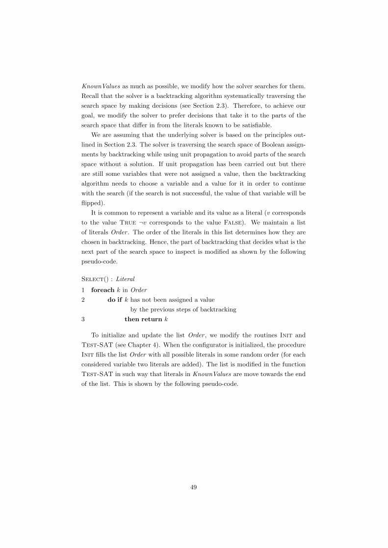
KnownValues as much as possible, we modify how the solver searches for them.
Recall that the solver is a backtracking algorithm systematically traversing the
search space by making decisions (see Section 2.3). Therefore, to achieve our
goal, we modify the solver to prefer decisions that take it to the parts of the
search space that differ in from the literals known to be satisfiable.
We are assuming that the underlying solver is based on the principles out-
lined in Section 2.3. The solver is traversing the search space of Boolean assign-
ments by backtracking while using unit propagation to avoid parts of the search
space without a solution. If unit propagation has been carried out but there
are still some variables that were not assigned a value, then the backtracking
algorithm needs to choose a variable and a value for it in order to continue
with the search (if the search is not successful, the value of that variable will be
flipped).
It is common to represent a variable and its value as a literal (v corresponds
to the value True ¬v corresponds to the value False). We maintain a list
of literals Order . The order of the literals in this list determines how they are
chosen in backtracking. Hence, the part of backtracking that decides what is the
next part of the search space to inspect is modified as shown by the following
pseudo-code.
Select() : Literal
1 foreach k in Order
2 do if k has not been assigned a value
by the previous steps of backtracking
3 then return k
To initialize and update the list Order , we modify the routines Init and
Test-SAT (see Chapter 4). When the configurator is initialized, the procedure
Init fills the list Order with all possible literals in some random order (for each
considered variable two literals are added). The list is modified in the function
Test-SAT in such way that literals in KnownValues are move towards the end
of the list. This is shown by the following pseudo-code.
49
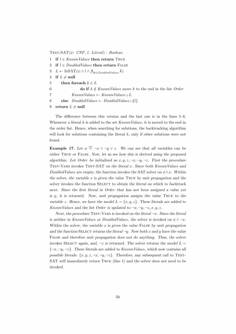
Test-SAT(ψ: CNF , l: Literal) : Boolean
1 if l ∈ KnownValues then return True
2 if l ∈ DisabledValues then return False
3 L← IsSAT(ψ ∧ l ∧∧k∈DisabledValues k)
4 if L 6= null
5 then foreach k ∈ L6 do if k /∈ KnownValues move k to the end in the list Order
7 KnownValues ← KnownValues ∪L8 else DisabledValues ← DisabledValues ∪{l}9 return L 6= null
The difference between this version and the last one is in the lines 5–6.
Whenever a literal k is added to the set KnownValues, it is moved to the end in
the order list. Hence, when searching for solutions, the backtracking algorithm
will look for solutions containing the literal k, only if other solutions were not
found.
Example 17. Let φdef= ¬x ∨ ¬y ∨ z. We can see that all variables can be
either True or False. Now, let us see how this is derived using the proposed
algorithm. Let Order be initialized as x, y, z,¬x,¬y,¬z. First the procedure
Test-Vars invokes Test-SAT on the literal x. Since both KnownValues and
DisabledValues are empty, the function invokes the SAT solver on φ∧x. Within
the solver, the variable x is given the value True by unit propagation and the
solver invokes the function Select to obtain the literal on which to backtrack
next. Since the first literal in Order that has not been assigned a value yet
is y, it is returned. Now, unit propagation assigns the value True to the
variable z. Hence, we have the model L = {x, y, z}. These literals are added to
KnownValues and the list Order is updated to ¬x,¬y,¬z, x, y, z.Next, the procedure Test-Vars is invoked on the literal ¬x. Since the literal
is neither in KnownValues or DisabledValues, the solver is invoked on φ ∧ ¬x.
Within the solver, the variable x is given the value False by unit propagation
and the function Select returns the literal ¬y. Now both x and y have the value
False and therefore unit propagation does not do anything. Thus, the solver
invokes Select again, and, ¬z is returned. The solver returns the model L =
{¬x,¬y,¬z}. These literals are added to KnownValues, which now contains all
possible literals: {x, y, z,¬x,¬y,¬z}. Therefore, any subsequent call to Test-
SAT will immediately return True (line 1) and the solver does not need to be
invoked.
50

4.5 Producing Explanations
There are different types of explanations that a configurator can provide. The
most basic type is the set of user decisions that necessitated a certain variable to
be locked. This can be made more informative by also including the explanation
parts of the initial formula responsible for the lock. Using a SAT solver enables
even more than these two types: the explanation is a tree of resolutions (see
Section 2.1.3) with the leaves forming a subset of the user decisions and parts
of the initial formula. Note that the tree contains both the decisions and parts
of the initial formula that are responsible for a certain variable to be locked,
but also, logical dependencies between them. Hence, we treat explanations as
trees of resolutions. Note that the two, less informative, types of explanations
can easily be obtained from such tree.
As the main objective of this dissertation is to develop configurators for fea-
ture models, it is assumed that the initial formula is a conjunct of formulas
corresponding to the individual modeling primitives (see Section 2.4.3), which
have been further translated into sets of clauses. Therefore, once the tool iden-
tifies the clauses in the explanation, it can track them back to the primitives
and display those to the user; this translation is discussed in greater detail in
Chapter 7. In this chapter, explanations are constructed from user decisions
and clauses coming from the initial formula.
Recall that a tree of resolutions is a tree representing a repeated application
of the resolution rule and that the root is a consequence of the leaves of that
tree (Section 2.1.3). Hence, explanations are defined as resolution trees.
Definition 6. Let φ0 be a CNF formula and D be a set of literals corresponding
to user decisions such that φ0 ∧∧d∈D d |= l for some literal l. An explanation
for φ0 ∧∧d∈D d |= l is a tree of resolutions with the root being l and each leaf
being a clause from φ or a literal from D.
An explanation is a resolution tree certifying that a certain variable
must be locked. The leaves of this tree are user decisions and parts of
the initial formula.
4.5.1 From Refutation to Explanation
An explanation for l can be requested only if φ∧ l has been shown to be unsatis-
fiable, where φ is the current state formula (Section 4.1). If that is the case, the
configurator can send a request for a refutation of φ∧ l by sending the message
Refute to the SAT solver. The refutation is a resolution tree where each of
the leaves is a clause from the state formula φ or the unit clause l; the tree’s
root is the empty clause ⊥.
51
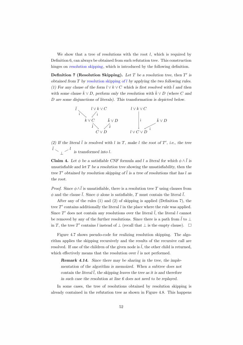
We show that a tree of resolutions with the root l, which is required by
Definition 6, can always be obtained from such refutation tree. This construction
hinges on resolution skipping , which is introduced by the following definition.
Definition 7 (Resolution Skipping). Let T be a resolution tree, then T ′ is
obtained from T by resolution skipping of l by applying the two following rules.
(1) For any clause of the form l ∨ k ∨ C which is first resolved with l and then
with some clause k ∨D, perform only the resolution with k ∨D (where C and
D are some disjunctions of literals). This transformation is depicted below.
l l ∨ k ∨ C
k ∨ C k ∨D
C ∨D
i i
j j
l ∨ k ∨ C
l ∨ C ∨D
k ∨Di
i
(2) If the literal l is resolved with l in T , make l the root of T ′, i.e., the tree
⊥l l
is transformed into l.
Claim 4. Let φ be a satisfiable CNF formula and l a literal for which φ ∧ l is
unsatisfiable and let T be a resolution tree showing the unsatisfiability, then the
tree T ′ obtained by resolution skipping of l is a tree of resolutions that has l as
the root.
Proof. Since φ∧ l is unsatisfiable, there is a resolution tree T using clauses from
φ and the clause l. Since φ alone is satisfiable, T must contain the literal l.
After any of the rules (1) and (2) of skipping is applied (Definition 7), the
tree T ′ contains additionally the literal l in the place where the rule was applied.
Since T ′ does not contain any resolutions over the literal l, the literal l cannot
be removed by any of the further resolutions. Since there is a path from l to ⊥in T , the tree T ′ contains l instead of ⊥ (recall that ⊥ is the empty clause).
Figure 4.7 shows pseudo-code for realizing resolution skipping. The algo-
rithm applies the skipping recursively and the results of the recursive call are
resolved. If one of the children of the given node is l, the other child is returned,
which effectively means that the resolution over l is not performed.
Remark 4.14. Since there may be sharing in the tree, the imple-
mentation of the algorithm is memoized. When a subtree does not
contain the literal l, the skipping leaves the tree as it is and therefore
in such case the resolution at line 6 does not need to be replayed.
In some cases, the tree of resolutions obtained by resolution skipping is
already contained in the refutation tree as shown in Figure 4.8. This happens
52

� ensures if tree contains a resolution over l,then result .resolvent = result .resolvent ∨l
� ensures if tree does not contain a resolution over l,then result = tree
Skip(tree : Tree; l : Literal) : Tree
1 if tree is a leaf then return tree2 child l ← Skip(tree.left , l)3 childr ← Skip(tree.right , l)4 if childr . resolvent = l then return child l5 if child l . resolvent = l then return childr6 return Resolve(childr, child l)
Figure 4.7: Realizing resolution skipping
x ¬x ∨ y ¬y ∨ z ¬z
y
z
⊥
11
2
2
3
3
A refutation of φ∧¬z, which shows that
φ |= z. The dashed rectangle marks the
part of the tree of resolutions obtained
by resolution skipping of z.
Figure 4.8: A resolution tree used to explain a locked variable
whenever the resolution over l is the last one in the resolution tree, i.e., it is the
resolution yielding the resolvent ⊥. The following example shows that resolution
skipping may lead to more complex transformations.
Example 18. Let us consider the following state formula φ
¬p ∨ ¬r ∨ ¬q¬p ∨ r ∨ ¬qp
It holds that φ |= ¬q. The tree on the left below refutes φ ∧ q and the tree on
the right is the corresponding explanation obtained by resolution skipping.
⊥
¬p¬p ∨ ¬r
¬p ∨ ¬r ∨ ¬q q
¬p ∨ r¬p ∨ r ∨ ¬q
p¬q
¬p ∨ ¬q
¬p ∨ ¬r ∨ ¬q ¬p ∨ r ∨ ¬q
p
53

Remark 4.15. If T ′ is obtained from T by resolution skipping, it
may be that T ′ contains clauses containing both the literal l and l,
which semantically corresponds to True. For illustration look at
the trees below; the one on the left is before resolution skipping and
the one on the right after:
l l ∨ y ∨ x
y ∨ x x ∨ l
y ∨ l y
l l
⊥
1 1
2 2
3 3
4 4
l ∨ y ∨ x
x ∨ l
l ∨ y ∨ l l ∨ y
l ∨ l l
l
1
1
2 2
3 3
Logically, the inference is correct but there are some redundant steps.
The proof obtained from the solver derives l from l in a complicated
fashion. The tree obtained by skipping infers l from True and l,
hence that part of the subtree can be dropped—in this case we obtain
a single-node tree as l was part of the formula. In general we drop the
trees that derive True as well all the resolution steps that become
invalid because of that.
An explanation in the form of a tree of resolutions can be obtained from
a refutation tree by resolution skipping.
4.5.2 Reconstructing Resolution Trees and The Catalyst
Optimization
If the catalyst optimization is used, the algorithm Test-Vars conjoins to the
state formula previously inferred literals (see line 4 in Figure 4.5). Therefore,
the proof returned by the solver may rely on these literals—meaning that they
appear in the leaves. This poses a problem for producing explanations as these
literals might not be part of the state formula, which comprises the initial for-
mula and user decisions. Recall that we require the explanation to have in the
leaves only clauses from the state formula (see Definition 6).
Hence, we need to reconstruct the resolution tree so that the catalyst literals
are no longer in the leaves. This is illustrated by the following example.
Example 19. Let φdef= (x⇒ y) ∧ (y⇒ z) ∧ x where x is the only user decision.
The procedure Test-Vars calls the solver with the query φ ∧ ¬y, which is
unsatisfiable and therefore φ |= y. In the next iteration the procedure calls
54

the solver with φ ∧ y ∧ ¬z to determine whether z can be False, to which the
solver responds negatively. As the solver has the previously inferred literal y
at its disposal, the proof it returns relies only on y, y⇒ z, and ¬z. Since y is
inferred and not given by the user, the configurator must add the explanation
for y. The resolution trees obtained from the refutations are depicted below in
the first row. The tree on the left shows that φ ∧ ¬y is unsatisfiable and the
tree on the right shows that φ ∧ y ∧ ¬z is unsatisfiable.
⊥x ¬x¬y x⇒ y
⊥¬z z
y y⇒ z
y
x x⇒ y
⊥¬z z
y
x x⇒ y
y⇒ z
At this point the tree refuting φ∧y∧¬z does not satisfy the requirements on
the leaves stated earlier (see Definition 6) as the leaf y is neither a user decision
nor part of the initial formula. It is necessary to merge the two trees in order
to justify y in the explanation of z.
To construct the tree required in the example above, we perform the two
following steps. (1) We perform resolution skipping for φ∧¬y so that y becomes
the root (instead of ⊥). (2) We attach this transformed tree to the resolution
tree for φ∧y∧¬z in order to justify y. The tree obtained in step (1) is depicted
the second row above on the left and how it is attached in step (2) is on the
right.
� requires φ ∧ l1 ∧ · · · ∧ lk ∧ l is unsatisfiable� requires φ ∧ l1 ∧ · · · ∧ li is unsatisfiable for i ∈ 1..kReconstruct(l1, . . . , lk : Literal ; l : Literal) : Tree
1 T ← Refute(φ ∧ l1 ∧ · · · ∧ lk ∧ l)2 L← {li | i ∈ 1..k and li is a leaf in T}3 foreach li ∈ L4 do Ti ← Reconstruct(l1, . . . , li−1; li)5 T ′i ← Skip(Ti, li)6 Replace the leaf li in T with T ′i7 return T
Figure 4.9: Justifying previous inferences in an explanation
To conclude, let us show how a refutation tree for φ ∧ l is reconstructed in
general. The situation we consider is that φ∧l1∧· · ·∧lk∧ l is unsatisfiable, where
55
l1, . . . , lk are previously inferred catalyst literals in this order. The pseudo-code
in Figure 4.9 shows how to compute the resolution tree for l that has none of
the l1, . . . , lk in the leaves. The function Reconstruct first asks the solver for
a resolution tree, which might contain the undesired leaves (line 1). For each
such leaf it constructs a refutation with a recursive call (line 4) and performs
resolution skipping (line 5) so it contains the literal li as the root by calling
the function Skip (see Figure 4.7). The transformed tree is then used as a
justification of the leaf (line 6).
Remark 4.16. Since any literal li can appear in the explanation of
li+1..lk multiple times, the implementation of Reconstruct should
be memoized.
If the catalyst optimization is used, the catalyst literals in the leaves of
the resolution tree need to be replaced with their explanations.
4.5.3 Notes on Explanation Size and Complexity
The explanations are constructed using resolution trees obtained from a SAT
solver. One issue with such a tree is that it might not be minimal. That is,
minimal in its size or even in the sense that removing certain clauses or user-
decisions still yields an unsatisfiable formula. Naturally, for the user-friendliness
sake, it is desirable for the explanation to be small. There is a significant amount
of research on obtaining small proofs and the reader is referred to the chapter on
related work for further references (Section 10.1.2). Any of these techniques can
be applied to make the explanations smaller. The implementation pertaining to
this dissertation uses for proof minimization the QuickXplain algorithm [111],
which is built in the solver SAT4J, and the tool MUSER [140] (see Section 7.1
for more details).
Another related question is whether it is not possible to provide explanations
with a simpler mechanism than resolution trees. Unit propagation provides ways
how to implement a non-backtrackfree configurator. In such configurator the
explanation mechanism can be implemented in an elegant way [15] (see also
Section 10.1).
This might suggest that explanations could be provided by reusing this tech-
nique. However, since unit propagation in general does not infer all bound
literals, such approach would require adding to the formula some information
obtained from the SAT solver. One possibility is to add the bound literals
obtained by using a SAT solver. The issue with this approach is that an expla-
nation for a certain bound literal obtained from unit propagation will comprise
that literal and nothing else. Hence, we would be getting explanations that are
not useful.
56
A more general issue relates to a result by Cook and Reckhow according
to which proofs are super-polynomial in size of the original formula unless
co-NP 6=NP [42]. Since unit propagation always performs a polynomial number
of steps, it means that for unit propagation to be able to infer any possible
bound literal, a super-polynomial information must be added.
From the theoretical perspective, proofs, and therefore explanations,
must be in general super-polynomially large. However, proof-
minimization techniques can be applied to mitigate this problem.
4.6 Summary
This chapter shows how to utilize a SAT solver to implement a complete and
backtrack-free configurator. The state of the configuration is maintained in
the state formula, which is a conjunct of the semantics of the instance being
configured and current user decisions. The algorithm hinges on propositions
established in Chapter 3; namely, that a literal is bound if and only if conjoining
the complementary literal with the state formula yields an unsatisfiable formula.
A simple algorithm is constructed from this proposition that invokes a SAT
solver on each considered literal (Section 4.2). This algorithm is made more
efficient by availing of the fact that a SAT solver returns a satisfying assignment
for satisfiable queries (Section 4.3).
Section 4.4 shows how to integrate in the algorithm an optimization that
by Kuchlin and Kaiser used in the context of non-interactive computation of
bound literals. This optimization modifies the order in which the underlying
SAT solver traverses the search space of variable assignments and it is aimed at
reducing the number of calls to the solver.
Section 4.5 how to provide explanations to the user why a certain variable
was locked in a certain value. Explanations are defined as trees of resolutions
that are rooted in the literal to be explained. The leafs of such tree comprise the
clauses from the state formula responsible for the lock and the internal nodes
are chains of reasoning for the locked literal from these leaves. It is shown
that such tree can always be obtained from a resolution tree returned by the
underlying solver (Figure 4.7). Since not all SAT solvers provide resolution trees,
an alternate solution for obtaining them is described in the chapter concerned
with implementation (Section 7.1).
In summary, this chapter makes the two following contributions: algorithms
that enable us to construct a backtrack-free and complete configurator using a
SAT solver and algorithms that enable us to construct explanations for why a
certain decision is disabled from resolution trees.
57

Chapter 5
Bi-Implied Set
Optimization
This chapter describes a syntactic-based optimization aimed at reducing the
number of satisfiability tests in the procedure Test-Vars (Figure 4.3). This
optimization is a variation of another optimization known in the feature model-
ing community as atomic sets [207, 180]. Atomic sets are equivalence classes of
features formed by the rule that a mandatory subfeature is in the same atomic
set as its parent. The features in an atomic set always all appear in a permissible
configuration or not at all, since a mandatory feature must be selected whenever
its parent is. Thus, it is sufficient to consider only one of the features from each
atomic set when analyzing the model, effectively collapsing the atomic sets. Ac-
cording to experimental research of Segura, collapsing atomic sets significantly
reduces computation time of analyses [180].
We observe that the FODA semantics (Section 2.4.3) prescribes that vc⇔ vf
if c is a mandatory child of f where vc, vf are the corresponding variables.
Hence, the variables corresponding to the features in an atomic set all have
the same value in any satisfying assignment of the formula representing the
semantics of the feature model. This motivates us to generalize atomic sets into
the context of CNF by focusing on equivalent literals, which are established by
the following definition.
Definition 8 (Equivalent literals). Given a formula φ, we say that the lit-
erals l and l′ are equivalent in φ if and only if under every satisfying assignment
of φ the literals l and l′ evaluate to the same value (both are either True or
both False). In mathematical vernacular φ |= l⇔ l′.
58

Remark 5.17. If a formula is unsatisfiable, i.e., has no satisfying
assignments, all pairs of literals are equivalent. However, as we are
interested in configuring satisfiable formulas, this is not practically
important.
Recall that the configurator described in the previous chapter determines
which literals are bound in the current state formula by using satisfiability tests
(see Test-Vars in Figure 4.3). The optimization developed in this section
collapses equivalent literals in order to decrease the number of these satisfiability
tests. The following observation shows that this is possible.
Observation 5. Let φ be a formula and l, l′ be literals equivalent in φ, and
let φ′ be φ with the literal l′ substituted by l. Then the formulas φ and φ′ are
equisatisfiable.
Proof. If there is satisfying assignment for φ, then this assignment is also satis-
fying for φ′ because l and l′ evaluate to the same value under this assignment.
If there is a satisfying assignment for φ′, this can be extended into a satisfying
assignment of φ by assigning such value to the variable in l′ that l and l′ evaluate
to the same value.
The observation above tells us that to compute the satisfiability of φ ∧ lifor some set of equivalent literals l1, . . . , ln, it is sufficient to consider only one
of the literals since all the other literals yield the same result. Clearly, it is
beneficial to identify sets of equivalent literals that are as large as possible. In
general, however, identifying equivalent literals is expensive complexity-wise as
shown by the following claim.
Claim 5. Determining whether two literals are equivalent in a given formula
is co-NP hard.
Proof. Let φ be a formula. We show that the test for whether φ is a tautology
can be converted to a literal equivalence test. Let x and y be variables not
appearing in φ and let φ′def= (φ⇔x) ∧ y. If φ is a tautology, then any variable
assignment of the variables in φ can be extended to a satisfying assignment of
φ′ where both x and y are True, and, these are the only satisfying assignments
of φ′. Note that if x and y appeared in φ, it would not be guaranteed that
any satisfying assignment of φ can be extended to φ′, e.g., for φ ≡ ¬x ∨ x or
φ ≡ ¬y ∨ y.
Conversely, if x is True in every model of φ′ then φ must be a tautology.
Consequently, φ is a tautology iff x is True in all models of φ′. And, since y is
True in all models of φ′, the literals x and y are equivalent iff φ is a tautology.
59
In summary, deciding the equivalence of x and y solves a co-NP-complete
problem and the reduction took polynomial time and thus the problem of literal
equivalence is co-NP hard.
Discouraged by the above claim, we look only for some pairs of equivalent
literals—for which it is easier to tell that they are equivalent. For inspiration we
look again at atomic sets. The semantics for mandatory subfeature yields the
bi-implication vf⇔ vc, which is equivalent to (vf⇒ vc) ∧ (vc⇒ vf ). Another
way of seeing this last formula is that these are two literals implying each other.
Hence, instead of just exploiting the mandatory relation, we consider literals
and implications between them. If literals imply each other, then they are
equivalent. Moreover, literals in a cycle of implications are equivalent due to
transitivity of implication.
To obtain implications from a CNF formula, we observe that every two-literal
clause corresponds to two implications.
Observation 6. Any clause comprising two literals corresponds to two impli-
cations, which are contrapositives of each other.
Example 20. The formula (x∨ y)∧¬z contains two clauses. The clause x∨ ycorresponds to the implications ¬x⇒ y and ¬y⇒x.
The set of implications obtained from two-literal clauses give rise to a graph
on the literals. This graph is defined as follows.
Definition 9 (Implication graph). The implication graph [7] of a CNF for-
mula ψ is obtained by introducing the vertices x and ¬x for each variable x
appearing in ψ and adding the edges⟨l1, l2
⟩and
⟨l2, l
⟩for all clauses of the
form l1 ∨ l2 in ψ.
Remark 5.18. Recall that l denotes the complementary
(“negated”) literal of l (see Section 2.1.3). The implication graph
construction ignores clauses with less or more than two literals.
In the following discussion we utilize the graph theory concept strongly con-
nected components. Recall that a strongly connected component (SCC) in a
directed graph is a maximal subgraph in which there is a path between each
two nodes of that subgraph.
Definition 10 (Bi-Implied Sets). In the context of a formula φ, bi-implied
literals are literals that appear in the same SCC of the implication graph of φ.
We call the SCCs of an implication graph bi-implied sets (BISs)
The following examples illustrate the defined terms. Note that the examples
in this section treat CNF formulas as a set of implicitly conjoined clauses in
60

order to avoid cluttering the text.
Example 21. The following set of clauses determines an implication graph
comprising two BISs depicted on the right.
¬a ∨ ¬b e ∨ d¬a ∨ ¬d ¬e ∨ ae ∨ b ¬b a ¬d
e
b ¬a d
¬e
Example 22. Consider the formula q ∧ x ∧ x⇒(y⇒ z) ∧ x⇒(y⇒ z) corre-
sponding to the set of clauses {q, x,¬x ∨ ¬y ∨ z,¬x ∨ ¬z ∨ y}. The literals q
and x are equivalent. In fact, they are both bound in the formula—they are
always True due to the unit clauses q and x. The literals y and z are equiva-
lent because they imply each other under the condition that x is True, which
is always fulfilled. However, none of the equivalent literals are in the same BIS.
The following observation summarizes the message of the examples above.
Observation 7. The literals in the same BIS of the formula φ are equivalent
in φ. However, there may be literals that are equivalent and are not in the same
BIS.
Example 23. Consider the fragment of a feature diagram depicted below
(adorned with the connectives corresponding to the semantics). There are two
atomic sets: {x, y} and {w}. However, we can detect that x, y, and w are
equivalent by looking at the implication graph (they are all in the same BIS).
x
y w
⇔⇐
requires (⇒)
Observation 8. The literals corresponding to variables in an atomic set always
belong to the same BIS. However, there may be other literals in such BIS.
Note that the two BISs in Example 21 are dual to one another: edges are
reversed and literals complemented. That is not a coincidence, the reason for
that is that each two-literal clause corresponds to two dual implications (con-
trapositives).
Observation 9. For any satisfiable formula and for each variable v there is a
BIS containing the literal v and a dual BIS containing the literal ¬v, where a
dual BIS is obtained by reversing all the edges and replacing the literals with
their complements.
61

Remark 5.19. If for a formula φ the literals v and ¬v are in the
same BIS, φ must be unsatisfiable since v and ¬v have the same
value in all models of φ, which is possible only if φ has no models.
See also Remark 5.17.
Observation 10. Computing BISs can be done in linear time of the size of the
formula since collecting the implications is a simple traversal of the formula and
computing the SCCs of the implication graph can be done in linear time [190].
Identifying Bi-Implied Sets (BIS) is a computationally cheap way of
identifying some, but not all, equivalent literals.
5.1 Performing BIS-Optimization
The BIS-optimization picks one literal from each BIS to represent the rest. This
literal is called the representative and in the rest of this section l 7→ r denotes
that the literal l is represented by the literal r. Since the literals in any BIS
are equivalent, replacing a literal with its representative yields an equisatisfiable
formula.
Example 24. Let φdef= {x⇒ y, y⇒ z, z⇒x, x ∨ y ∨ z}. Let x represent the
literals x, y, and z (which are in the same BIS of φ). In the context of φ,
instead of x ∨ y ∨ z, the BIS optimization performs computations on x.
As the goal is to minimize the number or variables, the optimization chooses
the representatives in such a way that:
1. All literals in the same BIS have the same representative.
2. Complementary literals are used to represent dual BISs.
Hence, for Example 21, the literal a will represent the BIS on the left if and
only if the literal ¬a represents the BIS on the right.
Remark 5.20. Collapsing literals sometimes causes clauses to col-
lapse as well. For instance, substituting y for x and ¬y for ¬x in the
CNF formula {x ∨ y,¬x ∨ y, y} yields the CNF formula {y}.
The following example in following illustrates how the BIS-optimization is
used in a configurator.
Example 25. Consider the CNF formula φdef= {f1⇒ f2, f2⇒ f1,¬f1∨¬f3, f3}.
As f1 and f2 imply one another, they fall into the same BIS. We choose f1 to
represent f2, i.e., f2 7→ f1, and perform the pertaining substitution, which yields
the formula {f1⇒ f1, f1⇒ f1,¬f1 ∨ ¬f3, f3}. The first two implications do not
affect the set of bound literals since both of the clauses are trivially True.
62

Hence, these implications are automatically discarded yielding the optimized
formula: φ′def= {¬f1 ∨ ¬f3, f3}.
Now we want to determine the satisfiability of φ ∧ f2. From the mapping
f2 7→ f1 we know that we need to ask the solver for the satisfiability of φ′ ∧ f1.
The SAT solver replies that φ′ ∧ f1 is unsatisfiable (¬f1 is bound in φ′). Hence,
φ ∧ f2 is unsatisfiable as well due to Observation 5 (¬f2 is bound in φ).
What if we want to know why ¬f2 is bound? Again, relying on the mapping,
we ask why ¬f1 is bound φ′. This can be explained using the clauses {¬f1 ∨¬f3, f3}. To relate the explanation to ¬f2, we also add the implication f2⇒ f1.
When initialized with the initial formula, the BIS-optimization computes the
BISs and records the choice of representatives. Then, whenever the satisfiability
of ψ needs to be determined, the satisfiability of ψ′ is computed instead, where
ψ′ is ψ with all literals substituted with their representatives (see also Obser-
vation 5). This is captured by the function Test-SAT-BIS (Figure 5.1) which
replaces the function Test-SAT in Test-Vars (Figure 4.3). The function first
performs the substitution of literals and then uses the original function Test-
SAT. Recall that Test-SAT never invokes the SAT solver more than once for
the given literal (Observation 2) and that the solver is not called more than
n + 1 times, where n is the number of variables (Claim 3). Hence, the BIS-
optimization does not call the solver more than n+ 1 where n is the number of
variables in the optimized formula.
Test-SAT-BIS(ψ: Formula, l: Literal) : Boolean
ψ′ ← substitute each literal with its representative in ψr ← representative of lreturn Test-SAT(ψ′ ∧ r)
Figure 5.1: Satisfiability testing with BIS-optimization
63

Remark 5.21. It is possible to integrate the BIS-optimization into
a SAT solver (see Section 10.2 for further references). However, if
that is the case, the effect is not the same as applying the optimiza-
tion upon initialization of the configurator. In the way we use the
optimization, not only the size of the formula is reduced, but also,
the solver is invoked fewer times—once we know whether a literal is
bound or not, we know that the same holds for all the literals in the
same BIS. Hence, if the solver implements the BIS-optimization in-
ternally, it is not as helpful. Firstly, in such case our algorithm calls
the solver the same number of times as if the optimization is not im-
plemented. Secondly, the solver needs to perform the optimization
each time it is invoked, while in our case it is performed just once.
As computing explanations in the BIS-optimization is more subtle, this is
discussed separately in the following section.
The BIS-optimization collapses literals occurring in the same Strongly
Connected Component of the implication graph.
5.2 Computing Explanations
To explain why a certain variable is bound, the configurator uses a resolution
tree (see Section 4.5). If the BIS optimization is used, the solver operates on the
optimized formula and knows nothing about the original, non-optimized version.
In particular, any resolution tree obtained from the solver is on the optimized
version. Therefore, in order to provide explanations on the non-optimized for-
mula, we need to reconstruct the resolution tree for the non-optimized formula
from the resolution tree for the optimized version.
φ ∧ l φ′ ∧ r
T T ′
optimize
refute refute
reconstruct
Figure 5.2: Depiction of reconstruction of a proof in the context of the BIS-optimization where T and T ′ are resolution trees refuting the respective formula
Let us look more closely at what happens (see Figure 5.2). Let φ be the non-
optimized formula and l be a literal such that φ∧ l is unsatisfiable (equivalently
φ |= l). If φ′ is the optimized version of φ and r is the representative of l, then
φ′ ∧ r is unsatisfiable as well (Observation 5). Therefore we can ask the solver
to give us a resolution tree for φ′ ∧ r and use it to build a tree for φ ∧ l.The basic idea for the tree reconstruction is that we keep the refutation of the
64

T ′
⊥
· · ·
T
A schematic depiction of the re-
construction of a tree from the
optimized formula. The resolu-
tion tree T ′ comes from reason-
ing on the optimized formula. The
smaller, filled trees come from the
BISs.
Figure 5.3: Proof reconstruction
optimized formula and enhance it with implications taken from the implication
graph as these relate the non-optimized to the optimized. What makes the
problem interesting is that it is not necessary to add all the implications as
illustrated by the following example.
Example 26. Let φdef= {¬x, x⇒ y, y⇒ z, z⇒x} and let x represent the literals
y and z, then the optimized version φ′ is {¬x}. Since φ′ ∧x is unsatisfiable and
x is the representative of z, then φ ∧ z is unsatisfiable. The refutation of φ′ ∧ x
is ⊥x ¬x
. To obtain a refutation of φ∧ z, it is sufficient to resolve z with
the implication z⇒x, to derive that the representative x holds while the rest
of the steps remain the same. This yields the following tree.
⊥x
z z⇒x¬x
In general, the tree reconstruction takes the tree refuting the optimized form
and prepends it with chains of implications for representatives appearing in the
optimized refutation (see Figure 5.3).
The following text explains the proof reconstruction in a top–down style.
The top-level function is BIS-Proof which produces a resolution tree for a
given formula and literal.
� requires φ ∧ l is unsatisfiable
BIS-Proof(φ : CNF ; l : Literal) : ResolutionTree
1 let φ′ be the optimized version of φ
2 let r be the representative of l
3 let T ′ be resolution tree for φ′ ∧ r4 T ← T ′
5 for each clause c that is a leaf in T ′ call SwapAll(c)
6 return T
The parameters of the function BIS-Proof are a CNF formula and a literal
such that the conjunction of the literal and the formula is unsatisfiable. The
function computes a resolution tree on the optimized version (line 3) and then it
65

calls the function SwapAll to prepend the leaves of that tree with appropriate
implications (line 5).
The function SwapAll used in BIS-Proof calls the function Swap multiple
times in order to derive a clause comprising the representatives of the literals in
the clause given to the function.
SwapAll(c : Clause) : Clause
c′ ← c
foreach l in c
do c′ ← Swap(c′, l)
return c′
The function Swap called on each literal of a clause in SwapAll constructs
a tree of resolutions that replaces a literal in the given clause with its represen-
tative. The pseudo-code assumes there is a function Resolve that performs a
resolution step on two given clauses and records it in the resolution tree T that
is being built by BIS-Proof (see above).
� requires l occurs in c� returns {r}∪ cr {l}, where l 7→ rSwap(c : Clause; l : Literal) : Clause
1 let r be a representative of l2 let P be a sequence of implications forming
some path from l to r in the implication graph3 c′ ← c4 k ← l5 � invariant: c′ ≡ {k}∪ cr {l}6 � invariant: the implications of P form a path from k to r7 while P 6= ∅8 do let ki ∨ ki+1 be the first element of P9 c′ ← Resolve(c′, ki ∨ ki+1)
10 let k ← ki+1
11 remove (ki ∨ ki+1) from P12 return c′
Since the functions above hinge on the function Swap we conclude with a
proposition proving correctness of Swap.
Proposition 4 (Literal Swap). The function Swap returns {l}∪ c r {r} as
expected.
Proof. The invariants are established before the loop is entered because c′ is
equal to c, the literal k is equal to l, and P forms a path from l to the literal r.
66

If P ≡ ki ∨ ki+1, ki+1 ∨ ki+2, . . . then the literal ki must be in the clause
c′ according to the invariant. Resolving c′ with ki ∨ ki+1 yields the clause
{ki+1}∪ c′ r {ki}. The resolution preserves the invariant because now P forms
a path from ki+1 to r and the literal ki+1 replaced ki in c′.
Since the invariant on the loop of Swap is correct and the loop terminates
when P is empty, the clause c′ must contain the literal r, which is the only
literal by which it differs.
To get the explanations for the original, non-optimized formula, some
implications from the implication graph are added to the explanation of
the optimized formula.
Computing Explanations with a SAT Solver
An alternative way of computing the explanation is to use the SAT solver again
on the unoptimized formula. This approach is less efficient and less predictable
but easier to implement than the one described above.
If the optimized formula φ′ ∧ r is unsatisfiable, then the original formula
φ ∧ l, where l 7→ r, is also unsatisfiable (Observation 5). Therefore calling the
solver on φ ∧ l will also yield a proof.
This approach is useful only when the explanations are needed significantly
less often than the other SAT queries otherwise that would defeat the purpose
of the optimization.
5.2.1 Choice of The Representative and Explanation Sizes
The BIS-optimization as described up to now, does not specify two important
things: (1) How to choose a representative of a BIS. (2) How to choose a path
from the literal to its representative in the proof reconstruction (Swap). This
section shows that both (1) and (2) affect the size of the explanations (resolution
trees), and suggests a strategy for them. The following example shows how
explanations vary depending on the choice of representative.
Example 27. Let φdef= {¬w ∨ ¬x ∨ ¬y ∨ ¬z, w}∪{x⇒ y, y⇒x, y⇒ z, z⇒ y},
which tells us that at least one of w, x, y, or z must be False. But also
that w is always True and that x, y, and z are equivalent. Therefore φ ∧ l is
unsatisfiable for l being any of the x, y, and z. Let us see what happens when
BIS-optimizations is applied. The BISs in the formula are the following.
w ¬w x y z ¬x ¬y ¬z
Let us assume that we want to show that z must be False, i.e., we need
a resolution tree using z and φ. We investigate two scenarios: one when the
67

representative for the literals {x, y, z} is the literal y and the other when the
representative is the literal x.
If y is chosen as the representative, φ is optimized into φ′ydef= {w,¬w ∨ ¬y}.
The following is the resolution tree for φ ∧ z where the dashed region marks
the resolution tree of φ′y ∧ y and the dotted regions are the added trees that
reconstruct the tree for φ∧z, i.e., the dotted sub-trees are obtained by invoking
SwapAll on the clause in the root of the sub-tree.
z z⇒ y
y
⊥
¬y
w ¬w ∨ ¬y
y⇒ z
y⇒x ¬w ∨ ¬x ∨ ¬y
¬w ∨ ¬x ∨ ¬y ∨ ¬z
T ′
In contrast, if x is chosen as the representative, φ is optimized into
φ′xdef= {w,¬w ∨ ¬x}. The following is also a resolution tree for φ ∧ z but re-
constructed from a tree for φ′x ∧ x.
z z⇒ y
y⇒xy
x
⊥
¬x
w ¬w ∨ ¬x
x⇒ z
x⇒ y
¬w ∨ ¬x ∨ ¬z
¬w ∨ ¬x ∨ ¬y ∨ ¬z
Note that the second tree requires one more resolution step to derive the
representative compared to the first tree (the first tree has 11 nodes and the
second 13). The reason is that to reach the representative x from z in the BIS
x y z requires two steps, whereas the representative y can be reached
from z in one step. The following table summarizes how the different choices
of representatives affect the size of the resolution tree. The rows correspond to
different choices of representatives; the columns correspond to different satisfi-
ability tests.
68
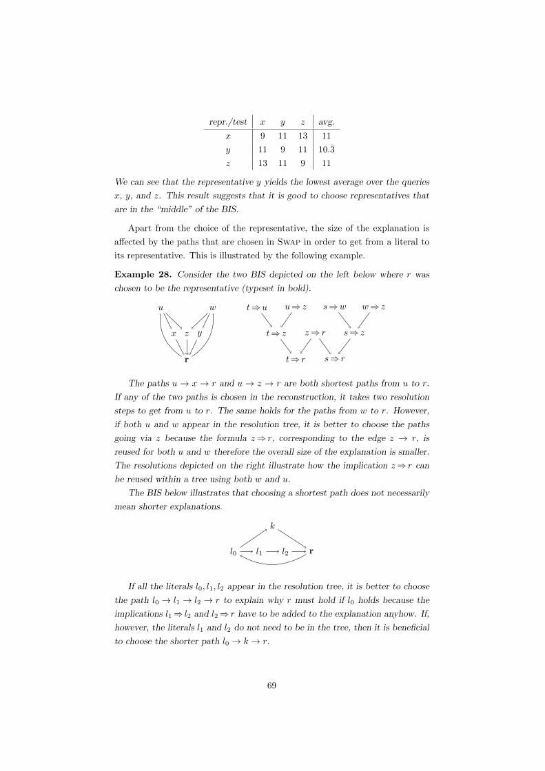
repr./test x y z avg.
x 9 11 13 11
y 11 9 11 10.3
z 13 11 9 11
We can see that the representative y yields the lowest average over the queries
x, y, and z. This result suggests that it is good to choose representatives that
are in the “middle” of the BIS.
Apart from the choice of the representative, the size of the explanation is
affected by the paths that are chosen in Swap in order to get from a literal to
its representative. This is illustrated by the following example.
Example 28. Consider the two BIS depicted on the left below where r was
chosen to be the representative (typeset in bold).
x
u
y
w
r
z
t⇒u u⇒ z s⇒w w⇒ z
t⇒ z z⇒ r s⇒ z
t⇒ r s⇒ r
The paths u → x → r and u → z → r are both shortest paths from u to r.
If any of the two paths is chosen in the reconstruction, it takes two resolution
steps to get from u to r. The same holds for the paths from w to r. However,
if both u and w appear in the resolution tree, it is better to choose the paths
going via z because the formula z⇒ r, corresponding to the edge z → r, is
reused for both u and w therefore the overall size of the explanation is smaller.
The resolutions depicted on the right illustrate how the implication z⇒ r can
be reused within a tree using both w and u.
The BIS below illustrates that choosing a shortest path does not necessarily
mean shorter explanations.
l0 l1 l2 r
k
If all the literals l0, l1, l2 appear in the resolution tree, it is better to choose
the path l0 → l1 → l2 → r to explain why r must hold if l0 holds because the
implications l1⇒ l2 and l2⇒ r have to be added to the explanation anyhow. If,
however, the literals l1 and l2 do not need to be in the tree, then it is beneficial
to choose the shorter path l0 → k → r.
69

From the examples above we know that both the choice of the represen-
tatives and the choice of paths from literals to their representatives affect the
size of explanations. The goal of this subsection is to find such strategies for
these choices that they yield, or are expected to yield, small resolution trees
on average. First let us focus on the problem of finding the paths with the
representatives fixed. The following proposition makes the problem easier by
revealing that it is sufficient to focus on each BIS separately.
Proposition 5. Let l be a literal represented by r in the BIS S and let S′ be a
BIS different from S, then there is no path connecting l to r going through S′.
In other words, a path from a l to r never leaves the BIS.
Proof. (by contradiction) Let l′ ∈ S′ such that the path from l to r goes
through l′. Then there are paths from l to l′ and from l′ to r. Since r and l
are in the same strongly connected component, there is also a path from r to
l. Therefore there is a path from l′ to r and a path from r to l′ via l, which
is a contradiction because that means that l′ and r are in the same strongly
connected component.
For the reconstruction of a resolution tree we need paths of implications
going from the literals in the non-optimized formula to their representatives
that appear in the optimized version. Therefore, the problem of minimizing the
resolution tree is to select such paths that use the fewest number of implications
in total. The above lemma tells us that paths going to different representatives
are disjunct. Therefore, if we can solve the problem for one BIS, then we can
solve it for the whole set of literals. The following problem restates the task in
graph-theoretical terms for one BIS.
Problem 1. Let G ≡ 〈V, E〉 be a directed graph, let r ∈ V and S ⊆ V . Find
a set E′ ⊆ E such that E′ contains a path for each n ∈ S to r.
This problem is the directed Steiner Tree Problem [38, Definition 1] and
is known to be NP-hard [38]. Therefore, we use a simple heuristic based on
shortest paths.
Definition 11 (Shortest Path Heuristic). Given an instance of Problem 1,
the Shortest Paths Heuristic chooses E′ as the union of some shortest paths
from the literals in S to their representatives. This is in mathematical notation
the following.
E′def= {P | P is some shortest path from l to r, where l ∈ S and l 7→ r} (5.1)
To implement the Shortest Paths Heuristic, we just need to refine Swap so it
identifies a shortest path from the given literal to its representative and it does
70

so that the same path is always used for the same literal (see line 2 in Swap).
Remark 5.22. Since the representatives are chosen at the begin-
ning of the configuration process, the shortest paths for all the literals
can be computed once at the beginning and stored.
The Shortest Paths Heuristic motivates the heuristic we use to choose the
representatives. Since the size of the union of the shortest paths is bounded
by the sum of the sizes of the individual paths (Equation 5.1), we pick the
representative so that the expected distance to other nodes in the BIS is minimal.
(A distance between two nodes in a graph is the length of a shortest path.)
For a literal l in the BIS S, let dl denote the sum of distances from all k ∈ Sto l. Note that since any literal is reachable from all the literals in the same
BIS, the average path length is dl|S| .
Recall that each BIS S has a dual BIS S′ with reversed edges and negated
literals. One of the decisions made earlier about representatives was that l
represents S iff l represent S′. Therefore, to minimize the average distance to
the representative, we look for a literal whose complement performs well too.
Definition 12. The Shortest Average Path Heuristics (SAP Heuristics) is that
for each BIS S pick as the representative a literal l ∈ S with the minimal dl+dl.
Remark 5.23. In graph theory, a node minimizing the sum of
distances to all other nodes is called a median of the graph [150].
Observation 11. If the BIS S contains i implications, finding the numbers dl
can be done in O(|S| (|S|+ i)) time and O(|S|) space by repeated breadth first
traversals. As a side-effect, this produces shortest path trees that are used later
by the optimizer to quickly find the implications that need to be added to the
explanation.
Choosing the best representative in general is difficult but it is reasonable
to pick such representatives so the average distance to it from a random
node in the BIS is short.
5.3 Summary
The BIS-optimization is based on the fact that the literals in the same strongly
connected component of an implication graph are equivalent. This chapter
shows how to integrate the BIS-optimization in a configurator that is con-
structed as described in Chapter 4. The basic idea is to collapse literals in
the same strongly connected component of the implication graph, which is con-
structed upon initialization, and then query the solver for only one literal out of
the component; this literal is called the representative. The second half of this
71

chapter investigates how to reconstruct resolution proofs that where obtained
from a solver operating on the optimized formula. We show that the choice
of representatives may influence the size of the reconstructed resolution tree.
Finally, we propose a heuristics for choosing a representative that is aimed at
reducing the size of the reconstructed trees.
In summary, the contributions of this chapter are showing how to use the
BIS-optimization in interactive configuration and showing how to reconstruct
proofs for a non-optimized formula from the pertaining optimized formula. It
should be noted that while the BIS-optimization is well known in the SAT
community, the proof reconstruction appears to be neglected by the existing
research (see Section 10.2).
72

Chapter 6
Completing a Configuration
Process
The text in the previous chapter is concerned the user-support during the con-
figuration process. This chapter focuses on its completion. The motivational
question is: “Is it necessary for the user to give a value to each and every variable
to complete the configuration?”
The chapter starts by a general discussion on configuration completion and
considers several different categories of automated support for completion. A
concept of the shopping principle is introduced (Section 6.1).
The bulk of the chapter is formed by Section 6.2 which studies the implemen-
tation of the shopping principle in the context of propositional configuration. It
also shows links to concepts known from Artificial Intelligence (Section 6.2.4).
Section 6.4.2 generalizes the shopping principle in the context of general
constraints; this will however require a notion of preference. It is shown that
the shopping principle is indeed a special case of this general approach. Finally,
Section 6.5 summarizes the chapter.
6.1 Completion Scenarios and the Shopping
Principle
Recall that a configuration process is complete if all features are bound (Defi-
nition 3 and Observation 1). Let us investigate some scenarios of how this can
be achieved. We assume that the configuration is carried out with the aid of a
backtrack-free configurator (see Chapter 3) and therefore, any bound features
are automatically computed after each user decision.
Consider that the user is configuring the feature tree in Figure 6.1 using a
73

root
opt alt
alt1 alt2 alt3
Figure 6.1: Example feature model
backtrack-free configurator. The hatched area represents the features that are
already bound, and thus, the only features that are not bound are those that
explicitly appear in the figure. Let us assume that the configurator enables the
user to indicate that the features in the hatched area are actually those that are
interesting for the user and the rest should go away. Upon this indication, the
configurator automatically sets all the unbound features to False (eliminates
them). Such behavior of the tool would be in accord with the way that people
shop at a fruit stall: customers tell a stall-keeper the items they want. They do
not specify the items they do not want nor do they need to go over every item
in specify for it whether they want it or not.
At a fruit stall this is always possible because there are no dependencies
between the items. As we know, in feature models there are dependencies and
this mechanism cannot be always applied. Consider, for example, that the user
selects the feature alt and then indicates that he or she is done. The feature
opt can still be eliminated but one of the alt1, alt2, or alt3, must be selected
because alt requires so. Therefore, if some automated method is to assign
values to the unbound features, it must choose between these three features. It
might not be desirable for the tool to make such choices as it means making a
choice for the user—it would be overly smart.
Remark 6.24. The issues discussed in the two paragraphs above
were already noted by Batory in [15, Section 4.2]. Therefore, this
chapter is actually a response to the problem hinted therein.
The informal discussion above enables us to classify the ways how the user
can complete the process.
M (Manual completion). The user continues makes decisions up to the
point when all considered variables are bound, i.e., each variable has been as-
signed a value by the user or by a decision inferred by the configurator. The
disadvantage of this approach is that the user needs to fill in every single detail
and that is cumbersome especially if there are some parts of the problem that
74

are not of a high relevance to the user. The only assistance the tool provides
is the mechanism that infers new decisions or disables some decisions. We will
not discuss this case further.
A (Full blind automation). The users make decisions up to a point where
they believe they made the decisions important for them and invoke a function
that automatically computes some appropriate values for all the variables that
have not been bound yet. The disadvantage of this function is that it takes all
the control from the user, in other words, it is making choices for them.
A+ (Smart automation). As in A, the users make decisions up to a point
where they believe they decided what they needed and invoke a function that
is supposed to bind the rest. The function in this scenario, bounds only those
variables for which it would not mean making a choice for the user. If there are
some variables that cannot be bound like that, the tool highlights them and it
is the user who makes that choice.
In some sense, the scenario A+ is a more careful version of scenario A. In
both scenarios, the tool helps the user to complete the configuration process.
However, scenario A binds all variables, whereas A+ binds based on the rule:
the variables that are not bound are eliminated unless that would mean making
a choice for the user. In the remainder of this text it is referred to this rule as
the shopping principle.
Hence, if A is applied to Figure 6.1 after alt has been selected, one of the
alt1, alt2, and alt3 is selected. In contrast to that, if shopping principle is
applied in the same situation, the feature opt is eliminated, whereas the features
alt1, alt2, and alt3 are left for the user to choose from.
Remark 6.25. Scenario A can be investigated more finely as the
binding function can be directed by some cost functions such as min-
imization of the number of selected features.
In summary, there are two types of functions that the user may invoke at
any step of the process in order to signal that the process should be completed:
(A) a function that binds all the remaining variables; (A+) a function that
binds only variables for which this would not mean making a choice for the
user; we call this function a shopping principle function.
The shopping principle function eliminates unbound variables but tries
not to be overly smart when doing so.
75

6.2 Completing a Propositional Configuration
Process
Following the motivation above, this section focuses on the completion of a
configuration process in terms of propositional logic. The case A is straightfor-
ward, binding all the remaining unbound variables means finding a solution to
the state formula φi in step i. This is a classical satisfiability problem, which
can be solved by a call to a SAT solver or by a traversal of a BDD corresponding
to φi.
The scenario A+, however, is more intriguing. The shopping principle tells
us that what has not been bound should be eliminated, which means setting to
False, in terms of propositional logic. However, it is not always possible to set
all unbound variables to False. For instance, in u ∨ v we cannot set both u
and v to False—in this case the user must choose which one should be True.
If we consider the formula x⇒(y ∨ z), however, all the variables can be set to
False at once and no further input from the user is necessary.
Hence, translating the shopping principle into the language of propositional
logic, the objective is to maximize the set of variables set to False without
making any choices for the user, i.e., variables that can be eliminated safely.
Upon a request, the configurator will set the safely-eliminable variables to False
and highlight the rest as they need attention from the user. Still, however, we
have not established what it formally means to “make a choice for the user”;
this is done in the following section.
6.2.1 Eliminating Safely
We begin by a couple of auxiliary definitions that establish what it means for
a variable or set of variables to be eliminable. The reference formula, denoted
as φ, in the following definitions is assumed to be the state formula of the state
when the shopping principle function is invoked. We write V to do note the set
of considered variables.
Definition 13 (Eliminable Variable). For a formula φ and a variable v ∈ Vwe write E(φ, v) and say that v is eliminable in the formula φ iff there is a model
of φ in which the variable v has the value False.
In plain English, a variable is eliminable if it can be set to False. The
following definition generalizes this concept for a set of variables.
Definition 14 (Eliminable Set). For a formula φ and a set of variablesX ⊆ Vwe write E(φ,X) and say that X is eliminable in φ, iff there is a model of φ
where all the variables in X have the value False.
76

The following observations show a connection between satisfiability and elim-
inable variables.
Observation 12. A variable v is eliminable in φ iff Sat(φ ∧ ¬v).
Proof. Any model of φ assigning False to v is also a model of φ ∧ ¬v. Hence,
if v is eliminable in φ, then φ ∧ ¬v is satisfiable. Conversely, any model M of
φ ∧ ¬v is also a model of φ and v has the value False in M . Hence, if φ ∧ ¬vhas at least one model (it is satisfiable), then φ has a model with v having the
value False.
Observation 13. A set X is eliminable in φ iff SAT(φ ∧
∧v∈X ¬v
).
Proof. Analogous to the proof for previous observation.
Example 29. Let φdef= (u∨ v)∧ (x⇒ y), then the set {x, y} is eliminable in φ,
while the sets {u, v} and {u, v, x} are not.
In the example above we see that {u, v} is not eliminable but also that
{u, v, x} is not eliminable. Clearly, if a set is not eliminable, it cannot be
made eliminable by adding more variables; this property is summarized by the
following observation.
Observation 14. If a set X is not eliminable in φ then any superset of X is
not eliminable either.
The following definition utilizes the concept of eliminable sets to identify
variables between which the user must choose.
Definition 15 (choice set). The set of variables X ⊆ V is a choice set in φ
iff the two following conditions hold.
1. X is not eliminable in φ, i.e., ¬E(φ,X).
2. All of the proper subsets of X are eliminable, i.e., (∀Y ( X)(E(φ, Y )).
Note that the condition 1. in the above definition ensures that at least one
variable in a choice set must be True while the condition 2. ensures that the set
is as “tight” as possible—removing any variable yields a set where all variables
can be set to False at once.
Remark 6.26. The requirement for tightness of a choice set comes
from Observation 14: if it was only required that it is not possible
to eliminate the set X, any of its supersets would have the same
property and thus taking on unrelated variables.
Variables between which the user must choose form minimal sets of vari-
ables where at least one variable must be True.
77

The concept of choice enables us to define those variables that can be elim-
inated without making a choice for the user; these variables are called dispens-
able.
Definition 16 (Dispensable variables). A variable v ∈ V is dispensable in
a formula φ iff it does not belong to any choice set in φ. We write Υφ to denote
the set of all dispensable variables in φ.
Example 30. Let φdef= (u ∨ v) ∧ (x⇒ y). All the variables u, v, x, and y are
eliminable. The set {u, v} is a choice set because it cannot be eliminated while
each of its subsets is eliminable.
The only sets that are not eliminable and contain x or y must also contain u
and v, i.e., they are {u, v, x}, {u, v, y}, and {u, v, x, y}. However, none of these
sets is a choice set because it does not fulfill the tightness requirement as {u, v}is not eliminable.
Hence Υφ = {x, y}, i.e., the variables x and y are dispensable while the
variables u and v are not (though they are eliminable).
Remark 6.27. Dispensability treats True and False asymmetri-
cally. In the formula x⇒ y, it is not possible to eliminate y without
eliminating x, i.e., eliminating y forces x to False. This, however,
does not collide with dispensability because both x and y can be
eliminated at the same time.
In contrast, eliminating u in u ∨ v forces v to True and therefore
the set {u, v} is not eliminable and the variables u and v are not
dispensable.
Remark 6.28. In any formula of the form x1 ∨ · · · ∨ xn the set
{x1, . . . , xn} is a choice set because it is not eliminable but any of its
proper subsets is because it is sufficient for only one of the x1, . . . , xn
to be True. Therefore, none of the variables x1, . . . , xn are dispens-
able.
The following example illustrates how dispensable variables are applied in
the context of a configurator process.
Example 31. Let φ0 be defined as in the previous example: φ0def= (u ∨ v) ∧
(x⇒ y). The user invokes the shopping principle function. Since x and y are
dispensable, both are eliminated (set to False). The variables u and v are
highlighted as they need user’s attention. The user selects u, which results in
the formula φ1def= φ∧ u = u∧ (x⇒ y). The variable v becomes dispensable and
can be eliminated automatically. The configuration process is complete as all
variables are bound: x, y, and v are bound to False, u to True.
78

x X
y X
u X w ×
z ×
o × p ×
⇒ ⇐or
⇒
⇐
or⇒
⇐
or
(a) x, y, and u selected; the rest are dis-pensable
x X
y X
u X w ×
z X
o ? p ?
⇒ ⇐or
⇒
⇐or⇒
⇐
or
(b) x, y, u, and z selected; only w dis-pensable
Figure 6.2: Examples of situations with selected and dispensable variables. Se-lected variables are marked with X; dispensable variables are marked with ×;other variables are marked with ? .
Example 32. Figure 6.2 shows two incomplete configurations of a feature di-
agram. The examples are to show that the definition of dispensable variables is
in accord with the intuition behind feature diagrams. In Figure 6.2a, w is dis-
pensable because u is selected. Similarly, z is dispensable because y is selected.
More generally, if one variable from an or-group is selected, then all the other
variables in that group are dispensable.
Since z is dispensable, the variables o and p are dispensable. More generally,
if a variable is dispensable, then the subtree rooted in that variable becomes
dispensable, provided there are no constraints cross-cutting the tree hierarchy.
The situation is slightly different in Figure 6.2b where z is selected. Now
the semantics tells us that z ∧ (z⇒(o ∨ p)) and therefore o and p cannot be
eliminated, while each one separately is eliminable. Hence, {o, p} forms a choice
set, and, o and p are not dispensable. More generally, whenever a variable is
selected, the or-groups belonging to it become choice sets.
6.2.2 Eliminating Dispensable Variables
The shopping principle function is supposed to eliminate all dispensable vari-
ables. The definition of dispensability, however, does not directly say that this
is actually possible. Here we show that the set of dispensable variables is indeed
eliminable. The proof of such will require the following lemma.
Lemma 1. Let φ be a formula and X be a finite set of variables not eliminable
in φ, then there is a subset of X that is a choice set.
Proof. If all proper subsets of X are eliminable, then we are done because X is
a choice set as it is not eliminable while each of its subset is eliminable. If X
contains a proper subset X ′ ( X that is not eliminable then we repeat with X ′.
This process must eventually terminate because X is finite.
79

Now it is straightforward to show that dispensable variables can be elimi-
nated all at once.
Proposition 6. For a satisfiable φ, the set of dispensable variables is eliminable
in φ, i.e., E(φ,Υφ).
Proof. (by contradiction) Let us assume that Υφ is not eliminable then it must
contain a set X that must be decided due to Lemma 1. Since Υφ consists only
of dispensable variables, which cannot be members of any choice set, the set
X must be empty. But if the empty set is a choice set, then it must not be
eliminable. This is a contradiction to the fact that φ is satisfiable because the
empty set is eliminable iff φ is satisfiable due to Observation 13.
All the dispensable variables can be eliminated all at once.
6.2.3 Dispensable Variables and Minimal Models
Remark 6.29. This part of the dissertation relies mostly on the
concepts and notation introduced in Section 2.1.2. In particular that
M(φ) denotes the set of minimal models of φ and models of formulas
are treated as sets of variables with the value True.
This section shows a relation of dispensable variables to minimal models
(Section 2.1.2). This relation is used later on to compute dispensable variables.
We start with a lemma relating minimal models and eliminable sets.
Lemma 2. If a set of variables is eliminable, then there is a minimal model
with all these variables assigned to False. Equivalently, using the notation
introduced so far: if E(φ,X) then there is a minimal model M of φ such that
M ∩X = ∅.
Proof. Let M be a model of φ such that it assigns False to all x ∈ X, i.e.,
M ∩X = ∅; such model exists because E(φ,X) holds. If M is minimal, then we
are done. If M is not minimal, then there is a model M1 of φ smaller than M ,
i.e., M1 ( M . Because M1 was obtained from M by removing some variables,
it still holds that M1 ∩X = ∅. Therefore, the process can be repeated with M1.
Since the initial model M is finite then we must eventually find a minimal model
by repeating the process.
Claim 6. A variable v is dispensable iff it is False in all minimal models. In
notation: φ |=min ¬v.
Proof. To show that if v is dispensable then it is False in all minimal models
we prove the contrapositive: if there is a minimal model M assigning True to
v, then v is not dispensable. Let Y be the set of variables that are False in M
80
and let Xdef= Y ∪{v}. The set X is not eliminable because any model assigning
False to all variables in X would be smaller than M but M is minimal. Since
X is not eliminable, from Lemma 1, there must be a set X ′ ⊆ X that is a choice
set. Since the set X ′ ⊆ Y ∪{v} and Y is eliminable and X ′ is not, the set X ′
must contain the variable v. Hence, v is not dispensable as it belongs to a choice
set.
To prove the inverse implication, we prove by contradiction that if v is False
in all minimal models, then it must be dispensable. Let v be not dispensable
in φ and φ |=min ¬v. Because v is not dispensable there must be a set X such
that v ∈ X, ¬E(φ,X), and E(φ,Z) for any Z ( X (see definitions 15, 16). Let
Ydef= X r {v}, since Y is a proper subset of X, then E(φ, Y ). From Lemma 2,
there is a minimal model M that assigns False to all variables in Y . Because
v is False in all minimal models of φ, it must be False in M as well. This
contradicts the assumption that X is not eliminable because the model M shows
that the set X = (X r {v})∪{v} is eliminable.
Example 33. Let φ0def= (u∨v)∧(x⇒ y). The minimal models of the formula φ0
are {u}, {v}, hence φ0 |=min ¬x and φ0 |=min ¬y. Then, if the user invokes the
shopping principle function, x and y are eliminated, i.e., φ1def= φ0∧¬x∧¬y. And,
the user is asked to resolve the competition between u ∨ v, selects u, resulting
in the formula φ2def= φ1 ∧ u with the models {u} and {u, v} where only the
model {u} is minimal hence v is set to False as dispensable. The configuration
process ends because u has the value True and the rest are dispensable.
6.2.4 Dispensable Variables and Non-monotonic Reason-
ing
This section investigates the relation between dispensable variables and a sub-
domain of Artificial Intelligence known as non-monotonic reasoning. This rela-
tionship is not only of a theoretical significance but also of a practical one as it
opens other ways of computing dispensable variables (other than those that are
shown in this dissertation).
The first thing to be clarified is the term non-monotonic reasoning appearing
in the title of this section. Unlike in classic logic inference, in non-monotonic
reasoning an increase in knowledge does not necessarily mean an increase in
inferred facts. Non-monotonicity is observed on the set of dispensable variables
as well: adding more constraints neither implies that the set of dispensable
variables expands nor does it imply that it shrinks. The following example
illustrates this property.
Example 34. Consider φ0def= x⇒(y ∨ z). The only minimal model of φ is ∅,
81

which assigns False to all the three variables and therefore, all of them are
dispensable due to Claim 6. Using the |=min notation, we write φ0 |=min ¬x,
φ0 |=min ¬y, and φ0 |=min ¬z.Conjoining φ0 with x yields φ1
def= (x⇒(y ∨ z))∧x with the minimal models
{x, y} and {x, z}. Neither of the variables is dispensable now, which means that
the set of dispensable variables has shrunk when going from φ to φ1. In terms of
the relation |=min, it is no longer possible to infer what was possible before, i.e.,
φ1 2min ¬y, φ1 2min ¬z, and φ1 2min ¬x. Moreover, in the case of variable x we
obtain a fact contradictory to the previous one, i.e., φ1 |=min x.
Conjoining φ1 with the formula y yields φ2def= (x⇒(y ∨ z))∧x∧y, which has
the only minimal model {x, y} and the variable z becomes dispensable. Hence,
the set of dispensable variables has expanded when going from φ1 to φ2.
The relation · |=min · is closely tied to the concept of circumscription in-
troduced by McCarthy in the 60’s as a form of non-monotonic reasoning [143].
While McCarthy originally operated on first-order logic, there is also the concept
of propositional circumscription, which is closer to the topic of this dissertation
(see for example [36]).
A circumscription of a propositional formula φ is the set of all minimal mod-
els of φ and reasoning with circumscription means determining which state-
ments hold in all minimal models of a formula, i.e., determining the validity of
φ |=min ψ. Hence, to determine whether a variable is dispensable is in fact a
special case of a circumscription reasoning due to Claim 6.
Remark 6.30. Observe that the set of all models does shrink when
the formula is constrained while the set of minimal models may
shrink or expand. Since the classic relation φ |= ψ means that ψ is
True on all models while φ |=min ψ means that ψ is True in all min-
imal models of φ, the relation · |=min ψ behaves non-monotonically
and · |= ψ monotonically.
Another term related to circumscription is the Closed World Assump-
tion (CWA) coming from the field of logic programming and knowledge rep-
resentation. Roughly speaking, CWA is based on the idea that a fact should
not be inferred unless there is a justification for it.
The literature offers several definitions of CWA [36, 63]. The definition
most relevant to this dissertation is the one of the Generalized Closed World
Assumption (GCWA) introduced by Minker [152] (also see [36, Definition 1]).
The following two definitions introduce GCWA using the notation of this dis-
sertation.
Definition 17 (free of negation). A variable v is free of negation in the
82

formula φ iff for any positive clause B for which φ 2 B, it holds that φ 2 v ∨B.
A clause is positive if it contains only positive literals, i.e., it is in the form
x1 ∨ · · · ∨ xn where x1, . . . , xn are variables.
Definition 18 (GCWA). The closure C(φ) of φ w.r.t. GCWA is defined as
C(φ)def= φ∪{¬v | v is free for negation in φ}
The formula ψ holds in the formula φ under GCWA iff C(φ) |= ψ.
The following lemma rephrases the condition for free of negation in terms of
eliminable sets.
Lemma 3. A variable v is free of negation in φ iff it satisfies the condition: if
E(φ,XB) then E(φ,XB ∪{x}) for any set of variables XB .
Proof. First observe that φ 2 ψ iff φ∧¬ψ is satisfiable. This lets us rewrite the
definition “v is free of negation” as follows. If φ ∧∧x∈VB
¬x is satisfiable, then
φ∧¬v∧∧x∈VB
¬x is satisfiable. This can be further rewritten using the concept
of eliminable sets as: if E(φ,XB) then E(φ,XB ∪{x}) (see Observation 13).
The following claim relates dispensable variables to those that are free of
negation.
Claim 7. A variable v is dispensable in φ iff it is free of negation in φ.
Proof. Using Lemma 3 we show that v is dispensable iff it holds that if E(φ,X)
then E(φ,X ∪{x}).To show that if v is free of negation then it must be dispensable, we prove
the contrapositive, i.e., if v is not dispensable then it is not free of negation.
If the variable v is not dispensable, then it belongs to some choice set Y , in
particular it holds ¬E(φ, Y ) and E(φ, Y r {v}) and therefore v is not free of
negation because the condition is violated for the set Xdef= Y r {v}.
Conversely, if v is not free of negation, then there is a set X for which E(φ,X)
but not E(φ,X ∪{v}). Since X ∪{v} is not eliminable, then there is a set X ′
that is a subset of X ∪{v} and it is a choice set (Lemma 1). Because X itself
is eliminable in φ, the set X ′ must contain the variable v and therefore v is not
dispensable.
The following claim relies on research on circumscription done by Eiter and
Gottlob in order to show the complexity classification of computation of dis-
pensable variables.
Claim 8. To determine whether a variable is dispensable in the formula φ is
ΠP2 . This holds even if φ in CNF.
83

Proof. From Claim 6, v is dispensable iff φ |=min ¬v. See [63, Lemma 3.1] for
ΠP2 completeness of φ |=min ¬v.
6.3 Computing Dispensable Variables
Claim 6 gives us a way to compute dispensable variables from minimal models.
The claim tells us that a dispensable variable must be False in all minimal
models. If we have the set of all minimal models at our disposal, we can go
through all of them and mark all the variables having the value True in any of
them as non-dispensable. The function Dispensable in Figure 6.3 realizes this
idea.
Dispensable(φ : Formula, V: Set of Variable) : Set of Variable
1 M←MinModels(φ)2 R← V3 foreach M ∈M4 do R← RrM5 return R
Figure 6.3: Computing dispensable variables from minimal models
The procedure Dispensable initially assumes that all variables are dispens-
able (line 2) and then it iterates over all minimal models. If a minimal model
contains a variable x, i.e., it assigns True to x, then x is not dispensable (line 4).
Once the loop terminates, the set R contains only the dispensable variables.
What is missing at this point is an implementation of the function
MinModels that computes the set of all minimal models.
The algorithm used in this section to collect all minimal models is based on
the following loop: (1) Find some minimal model of the formula. (2) Disable
from the formula all models greater or equal to that minimal model. (3) If the
formula is still satisfiable then goto (1).
The step (2) shrinks the set of models of the formula in such way that the
model found in step (1) is the only minimal model taken out. Since every formula
has a finite number of minimal models eventually all of them are taken out, the
formula becomes unsatisfiable and the loop terminates. Figure 6.4 presents
pseudo-code for an implementation of the function MinModels realizing this
idea.
The heart of MinModels is the loop on lines 7–9. At the beginning of each
iteration it first records the minimal model found last (line 7), then it finds a
minimal model M (line 8) and strengthens the formula such that all models
84

MinModels(φ0 : Formula) : Set of Model
1 R← ∅2 φ← φ0
3 M ←MinModel(φ)4 � invariant: R∪M(φ) =M(φ0)5 � invariant: R∩M(φ) = ∅6 while M 6= null7 do R← R∪{M}8 M ←MinModel(φ)9 φ← φ ∧
∨v∈M ¬v
10 return R
Figure 6.4: Computing the set of minimal models
greater or equal to M are no longer models of φ (line 9).
M
The little circles at the bottom repre-
sent minimal models. The hatched area
represents the models removed from
the formula along with the minimal
model M .
Figure 6.5: Removal of models
The effect of line 9 is illustrated by Figure 6.5. The hatched area represents
the models removed by the strengthening. The models in this area must assign
True to all the variables that have the value True in M . Therefore the hatched
area corresponds to the formula∧v∈M v. Since this area is to be excluded, φ is
conjoined with the negation of this formula which is∨v∈M ¬v.
Example 35. Let φ0def= x∨ (y ∧ z) (the subscript in φi represents the different
iterations of the loop in MinModels). Let {x} be the first minimal model
found, then φ1def= φ0 ∧¬x according to line 9. The formula φ1 can be rewritten
equivalently as y ∧ z ∧ ¬x, which has a single minimal model {y, z}. Finally,
executing line 9 yields (y ∧ z ∧¬x)∧ (¬y ∧¬z), which has no (minimal) models
and the algorithm terminates.
Line line 9 of MinModels requires a function MinModel that computes
some minimal model of φ. To compute a minimal model we utilize a SAT solver,
which is described by Section 6.3.1. First, however, let us look more closely at
the properties of the procedure MinModels driving the process. The first
observation is concerned with the form of the formula guaranteeing that a SAT
solver can always be invoked.
85

Observation 15. If the input formula φ0 is in CNF, then φ is in CNF at all
times.
Proof. The initial formula φ0 is in CNF, and φ is conjoined with∨v∈M ¬v which
is a clause.
Observation 16. Line 9 removes from φ only models greater or equal to M .
Formally, let φ and φ′ denote the formulas before and after performing line 9,
respectively. Let M be the model found in line 8 and M ′ be some model of φ.
Then M ′ is not a model of φ′ iff M ⊆M ′.
Proof. If M ′ is a model of φ but is not a model of φ′, it must violate the newly-
added clause∨v∈M ¬v. That means that all the v ∈M are True in M ′, which
is equivalent to M ⊆ M ′. Conversely, if M ⊆ M ′ then M ′ is violating the
newly-added clause∨v∈M ¬v and therefore it is not a model of φ′.
Lemma 4. Line 9 removes one minimal model, which is M . Formally, let φ and
φ′ denote the formulas before and after performing line 9, respectively. Then,
M(φ′) =M(φ) r {M}.
Proof. We start by proving (M(φ)r {M}) ⊆M(φ′) by showing that any min-
imal model N of φ that is not equal to M , is a minimal model of φ′. Firstly, N
must not be a superset of M because it is a minimal model in φ. From which
it follows that N is a model of φ′ due to Observation 16. To show that N is
minimal model of φ′ by contradiction we assume there is a model N ′ of φ′ such
that N ′ ⊆ N . Since N is minimal in φ, the set N ′ must not be a model of φ
but that contradicts Observation 16 as models of φ′ are a subset of the models
of φ according to that observation.
Conversely we prove M(φ′) ⊆ M(φ) r {M} by showing that any minimal
model of φ′ is a minimal model of φ. Let N ∈ M(φ′), then N is a model of φ
as φ′ was obtained by strengthening φ. For contradiction, let us assume that N
is not a minimal model of φ. Then there is model N ′ of φ such that N ′(N and
N ′ is not a model of φ′. Since N ′ is not a model of φ′ but is a model of φ, it
must be M ⊆ N ′ due to Observation 16. Hence, we have M ⊆ N ′ and N ′ ⊆ N .
From transitivity of ⊆ we obtain M ⊆ N but that is a contradiction because
N is a model of φ′, which does not have models that are supersets of M due to
Observation 16.
Lemma 5. The loop invariants in MinModels on lines 4 and 5 hold.
Proof. The invariants R∪M(φ) = M(φ0) and R∩M(φ) = ∅ are trivially es-
tablished upon the entry of the loop as R is empty and φ is equal to φ0.
86

Let φ and R denote the values at the beginning of an arbitrary iteration of
the loop and φ′ and R′ at the end of the iteration. Due to Lemma 4, M(φ′) =
M(φ)r{M}, which gives us the following equalities that prove the first invariant
(M(φ0) = R′ ∪M(φ′)).
M(φ0) =induction hypothesis
R∪M(φ) =equivalence
(R∪{M})∪(M(φ) r {M}) =Lemma 4 and equivalence
R′ ∪M(φ′)
The second invariant is clearly preserved by the loop sinceM(φ) and R are
disjoint and therefore M(φ′) and R′ are disjoint as well.
Claim 9. When the algorithm MinModels terminates, it returns all minimal
models of the input formula φ0.
Proof. Since the invariant M(φ)∪R =M(φ0) holds and when the loop termi-
nates M(φ) is empty, R =M(φ0)
Claim 10. The algorithm MinModels is terminating. In particular it iterates
as many times as many minimal models there are in the input formula φ0.
Proof. From Lemma 4 we know that the loop decreases the number of minimal
models of φ by one. As the loops stops when φ has no minimal models, the loop
iterates as many times as many minimal models φ0 has.
6.3.1 Computing a Minimal Model with a SAT Solver
As shown in the previous section, we can enumerate the set of all minimal models
if we have the means to compute one minimal model. This section shows that a
SAT solver that is based on the principles outlined in Section 2.3 can be easily
modified to find a minimal model. Intuitively, the modification is to enforce the
preference of False over True as specified by the following definition.
Note that the term decision in this section refers to the decisions that the
solver makes to traverse the search space not the decisions that the user makes
to reach the current state formula.
Definition 19. We say that a SAT solver is biased to False iff the solver
always makes the decision ¬v before the decision v for each variable v.
Example 36. Let φdef= x∨y∨z be a formula given to a solver biased to False.
The solver makes the decision ¬x followed by the decision ¬y. At this point unit
propagation assigns True to z, resulting in the satisfying assignment ¬x,¬y, z.
87
Note that for any ordering of decisions a solver biased to False assigns False
to two of the variables and True to the remaining one.
The example above illustrates that solvers biased to False tend to find
solutions with as many False values as possible, roughly speaking. In fact, we
will see that they always return minimal models. To show that, we first make
an observation that if a biased solver ever assigns True to a variable, it must
do so unless some of the previous assignments are changed.
Lemma 6. Let φ be a satisfiable CNF formula to which a solution was found
by a SAT solver biased to False. Let l1, . . . , ln be literals corresponding to the
assignments made by the solver (l1 is the first decision and ln is the last), then
for any assignment for which li ≡ vi it holds φ |= (l1 ∧ · · · ∧ li−1)⇒ li.
Proof. There are two ways how the solver can assign a value to a variable: either
in unit propagation or by a decision.
If the assignment li ≡ vi was made by unit propagation then there exists a
clause k1 ∨ · · · ∨ kl ∨ vi such that the literals k1, . . . , kl evaluate to False under
the assignment l1, . . . , li−1. Hence, vi must have the value True.
If the solver made the decision li ≡ vi, then the formula must be unsatisfiable
under the assignment l1, . . . , li−1,¬vi due to Property 11 and due to the fact that
the solver must have tried the decision ¬vi before as it is biased to False.
Proposition 7. Let φ be a satisfiable CNF formula to which a solution was
found by a SAT solver biased to False. Let M be a satisfying assignment
returned by the solver represented by the literals l1, . . . , ln sequenced in the
order as the assignments were made by the solver, then M assignment is a
minimal model of φ.
Proof (by contradiction). Let M ′ be an assignment assigning False to some
variables to which M assigns the value True thus showing that the model M is
not minimal. Let vk be the variable from these variables assigned the first, i.e.,
M assigns True to vk and M ′ assigns False and there is no such other variable
assigned earlier. Since M ′ agrees with M on the assignments l1, . . . , lk−1, due
to Lemma 6 the assignment M ′ cannot be a model of φ.
Using a SAT solver it is possible to enumerate all minimal models and
thus identify the dispensable variables.
1The property tells us that once the solver assigned values to some variables, and, this as-signment is possible to complete into a satisfying assignment, such assignment will be returnedby the solver (see Section 2.3).
88

6.4 Completing Configuration Processes for
General Constraints
The previous section investigates how to help a user with the completion of a
configuration of propositional constraints, motivated by the shopping principle.
This section investigates how to generalize the principle for non-propositional
constraints.
The shopping principle function attempts to eliminate as many variables as
possible. This can be alternatively seen as that the user prefers the unbound
variables to be False (see also Remark 6.27). This perspective helps us to
generalize the approach to the case of non-propositional constraints under the
assumption that there is some notion of preference between the solutions.
First, let us establish the principles for preference that are assumed for this
section. (1) It is a partial order on the set in question. (2) It is static in the
sense that all users of the system agree on it, e.g., it is better to be healthy
and rich than sick and poor. (3) If two elements are incomparable according
to the ordering, the automated support shall not decide between them, instead
the user shall be prompted to resolve it.
6.4.1 Concepts for Non-propositional Configuration
The following definitions enable us to discuss the general case formally. We
start by a general definition of the instance to be configured, i.e., the initial
input to the configurator, corresponding to the set of possibilities that the user
can potentially reach. As in the propositional case, the user can make decision
about variables and the configuration is complete when all variables’ values are
determined. The difference is, however, that a variable can have a value from
a larger domain than just True and False. The following definition realizes
this intuition in mathematical terms (this definition is inspired by [101] and by
constraint satisfaction problem, see Section 2.1.4).
Definition 20 (Solution Domain). A Solution Domain is a triple 〈V, D, φ〉where V is a set of variables V = {v1, . . . , vn}, D is a set of respective domains
D = {D1, . . . , Dn}, and the constraint φ ⊆ D1 × · · · ×Dn is an n-ary relation
on the domains.
A variable assignment is an n-tuple 〈c1, . . . , cn〉 from the Cartesian product
D1 × · · · × Dn, where the constant ci determines the value of the variable vi
for i ∈ 1 . . . n. For a constraint ψ, a variable assignment α is a solution iff it
satisfies the constraint, i.e., α ∈ ψ.
Example 37. Let us have two hardware components with the respective con-
89
stant prices p1, p2 and a configurable maximum price. This can be modeled as
the following solution domain.
Let V def= {c1, c2, p}, D
def= {{0, 1}, {0, 1},N}, and the relation
φdef= {〈s1, s2, k〉 | (p1 · s1 + p2 · s2) ≤ k}
The solution domain expresses that the two components can be either in-
cluded or not and that the price of the included component(s) must be less than
the maximum price, which is a natural number.
It is easy to see that a propositional formula is expressible as a solution
domain by representing satisfying assignments of the formula by the solutions
of the solution domain.
Observation 17. Let φ be a propositional formula on a finite set of variables
V ≡ {v1, . . . , vn}. Let Didef= {False,True} for i ∈ 1 . . . n. Let ψ be relation on
D1 × · · · ×Dn defined as follows.
ψdef= {〈b1, . . . , bn〉 | the assignment assigning bi to vi
for i ∈ 1..n is a satisfying assignment of φ}
Then 〈V, {D1 . . . Dn}, ψ〉 is a solution domain such that there is a bijection
between its solutions and the satisfying assignments of φ.
A configuration process of a solution domain 〈V, D, φ〉 is defined in a fashion
analogous to the propositional case. The user actions are making a decision or
retracting one. A decision is an arbitrary constraint on the solution domain
being configured. In particular, if a decision ξj is of the form vi = c for a
variable vi and a constant c ∈ Di, we say that the variable vi has been assigned
the value c in step j.
The configuration process is represented as a sequence of sets of decisions
such that the first set is empty and subsequent ones are obtained by adding or
removing a decision. If Γi is the set of decisions in step i, the state constraint
is the set of solutions determined by the decisions, i.e., φ∩⋂ξ∈Γi
ξ. A variable
v is bound to the constant c in the state constraint φi iff all the solutions of φi
assign the value c to v. A configuration process is complete iff all the variables
in V are bound.
Note that the propositional configuration process is a special case of the
general one. In particular, selecting a variable means adding the constraint
x = True and eliminating a variable means adding x = False.
A backtrack-free configurator in this process disallows assigning values that
do not appear in any of the solutions of the current state constraint. More specif-
ically, in step l the configurator disallows all values c ∈ Di of the variable vi for
90
which there is no solution of the state constraint φl of the form 〈c1, . . . , c, . . . cn〉.For convenience, if the variable vi is bound to some value c (all values but c are
disallowed for the domain Di), then the configurator automatically assigns c to
the variable vi.
6.4.2 Configuration with Preference
Since this section requires the notion of preference, the definition of a solution
domain is extended to accommodate for such.
Definition 21 (Ordered Solution Domain). An Ordered Solution Do-
main (OSD) is a quadruple 〈V, D, φ, ≺〉 where 〈V, D, φ〉 is a solution domain
and ≺ is a partial order on the Cartesian product D1 × · · · ×Dn. For a con-
straint φ, a solution α is optimal iff there is no solution α′ of φ such that α′ 6= α
and α′ ≺ α.
Since an ordered solution domain is an extension of a solution domain, the
configuration concepts apply here as well. However, the extra information can
be exploited in order to help the user with completing the configuration process.
Let us assume that a user is configuring an ordered solution domain and we wish
to provide assistance with configuring variables that have lesser importance for
the user, similarly as we did with the shopping principle. Just as before, the
configuration proceeds as normal up to the point where the user configured
all those variables the user wanted to configure and then invokes a function
that tries to automatically configure the unbound variables using the given
preference.
The assumption we make here is that the variables that were not given a
value yet should be configured such that the result is optimal while preserving
the constraints given by the user so far. Since the preference relation is a partial
order, there may be multiple optimal solutions. As we do not want to make a
choice for the users, we let them focus only on optimal solutions.
If non-optimal solutions are ignored, the configurator can identify such values
that never appear in any optimal solution. Dually, the configurator identifies
values that appear in all optimal solutions, the following definitions establish
these concepts.
Definition 22 (Non-Optimal Values). For a constraint φ and a variable vi,
a value c ∈ Di is non-optimal iff the variable vi has the value c only in non-
optimal solutions of φ. Equivalently, the variable vi has a value different from
c in all optimal solutions of φ.
Definition 23 (Settled Values and Variables). For a constraint φ and a
variable vi, a value c ∈ Di is settled iff vi has the value c in all optimal solutions
91

of φ. A variable vi is settled iff there is some settled value of vi.
Non-optimal and settled values are related by the following observation.
Observation 18. For a constraint φ and a variable vi, a value c ∈ Di is settled
in φ iff all values c′ ∈ Di different from c are non-optimal in φ.
Example 38. Let x, y, z ∈ {0, 1}. Consider a constraint requiring that at least
one of x,y,z is set to 1 (is selected). And the preference relation will express
that we prefer lighter and cheaper solutions where x, y, and z contribute to
the total weight by 1, 2, 3 and to the total price by 10, 5, and 20, respectively.
Hence, the solutions satisfy (x + y + z > 0), and 〈x1, y1, z1〉 ≺ 〈x2, y2, z2〉 iff
(10x1 +5y1 +20z1 ≤ 10x2 +5y2 +20z2)∧(1x1 +2y1 +3z1 ≤ 1x2 +2y2 +3z2). Any
solution setting z to 1 is non-optimal as z is more expensive and heavier than
both x and y, and hence the configurator sets z to 0 (it is settled). Choosing
between x and y, however, needs to be left up to the user because x is lighter
than y but more expensive than y.
As noted in Observation 17, propositional configuration, can be seen as a
special case of a configuration of a solution domain with the variable domains
{True,False}. The following observation relates settled and dispensable vari-
ables (definition 23 and 16).
Observation 19. Let φ be a propositional formula and 〈ψ, V, D〉 be a
corresponding solution domain (see Observation 17), and let 〈b1, . . . , bn〉 ≺〈b′1, . . . , b′n〉
def=∧i∈1..n bi⇒ b′i. Then, a variable is dispensable in φ iff the value
False is settled in the ordered solution domain 〈ψ, V, D, ≺〉.
Proof. We note that when α ≺ β then if α assigns True to any variable, β
must do so as well. Hence, the ordering · ≺ · corresponds to the subset ordering
on the models of the formula φ. From Claim 6, a variable is dispensable iff it
is False in all minimal models. In terms of the ordered solution domain, the
variable has the value False in all the optimal solutions, i.e., False is settled
in φ.
6.5 Summary
This chapter shows how to extend a configurator with a function that helps the
user to complete the configuration process whenever invoked. In the case of
propositional configuration, this completion function is designed according to
the shopping principle (Section 6.2). The motivation comes from an analogy
with the shopping at a fruit stall: the customer is enumerating items he or she
wants. This process terminates when the customer decides he or she has all
92

that was needed. Hence, the person who is shopping never needs to go through
all the items in the stall and say for each item whether he or she wants it or
not. In the case of dependencies between the items, this is not that easy and
only certain items can be skipped and be not bought. The term dispensable
variables (Definition 16) is introduced to formally identify the variables that
can be eliminated (skipped) when the shopping principle function is invoked.
The chapter shows how to calculate these variables using a SAT solver in Sec-
tion 6.3. However, other ways for the calculation are opened by relating to
propositional circumscription and Closed World Assumption in Section 6.2.4;
for more information see Section 10.3 in the chapter on related work.
This chapter further generalizes the shopping principle to the case of non-
propositional configuration relying on the notion of preference (Section 6.4.2).
This generalization shows that the shopping principle can be seen as a preference
for not-buying even though such presentation might appear counter-intuitive at
first.
In summary, the contributions of this chapter are the following
• discussion and classification of possible scenarios of completion of config-
uration,
• formal definitions of the concept “making a choice between a set of user
decisions”,
• an algorithm that enables us to compute variables that can be eliminated
without making a choice for the user, and
• a formal connection between the concept of choice and the concept of
preference.
93
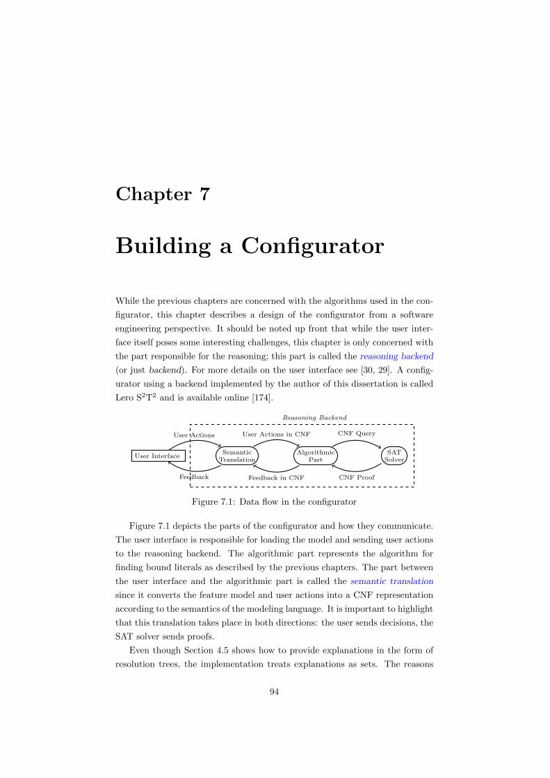
Chapter 7
Building a Configurator
While the previous chapters are concerned with the algorithms used in the con-
figurator, this chapter describes a design of the configurator from a software
engineering perspective. It should be noted up front that while the user inter-
face itself poses some interesting challenges, this chapter is only concerned with
the part responsible for the reasoning; this part is called the reasoning backend
(or just backend). For more details on the user interface see [30, 29]. A config-
urator using a backend implemented by the author of this dissertation is called
Lero S2T2 and is available online [174].
User Interface
Reasoning Backend
SemanticTranslation
AlgorithmicPart
SATSolver
User Actions
Feedback
User Actions in CNF
Feedback in CNF
CNF Query
CNF Proof
Figure 7.1: Data flow in the configurator
Figure 7.1 depicts the parts of the configurator and how they communicate.
The user interface is responsible for loading the model and sending user actions
to the reasoning backend. The algorithmic part represents the algorithm for
finding bound literals as described by the previous chapters. The part between
the user interface and the algorithmic part is called the semantic translation
since it converts the feature model and user actions into a CNF representation
according to the semantics of the modeling language. It is important to highlight
that this translation takes place in both directions: the user sends decisions, the
SAT solver sends proofs.
Even though Section 4.5 shows how to provide explanations in the form of
resolution trees, the implementation treats explanations as sets. The reasons
94

for this are rather technical, the SAT solver used (SAT4J) supports proofs only
in the form of sets of CNF formulas and the user interface does not support
visualization of explanations as trees.
An important design decision in the implementation of the backend is its
modularization. The modularization is guided by two main criteria: separation
of concerns and extensibility. Separation of concerns led to the decision that
the semantic translation is done in multiple steps, each step dealing with a
conceptually different type of translation. Each of these steps is implemented as
a separate component and thus can be easily replaced. Extensibility means that
it should be easy to add optimizations such as the BIS-optimization described
in Chapter 5.
The architecture of the backend is described in the following section (Sec-
tion 7.2). Section 7.3 describes the implementation of the backend, which follows
the architecture described in the upcoming section. Section 7.4 discusses the
advantages and disadvantages of the presented design.
7.1 Implementing Explanations
The implementation uses two different engines to compute explanations. One
is built into the solver SAT4J, which is used as the underlying solver for the
inference in the configurator. The second uses an external tool MUSER [140].
SAT4J uses the algorithm QuickXplain [111] to produce unsatisfiable cores
of the given formula. Such core comprises leaves of some resolution tree that
we need in order to provide explanations (see Section 4.5). To obtain such
resolution tree, another SAT solver (called PidiSAT) is called on the core of
clauses obtained from SAT4J. PidiSAT was developed by the author of this
dissertation and has the ability to produce resolution trees for unsatisfiable
inputs (unlike SAT4J). The reason why PidiSAT is not used in the inference
algorithms is that it is far less efficient than SAT4J. However, the efficiency
is not critical for constructing resolution trees because the solver is invoked
on a significantly smaller set of clauses than the original problem. PidiSAT is
available for download at Kind Software website [102]. The following example
shows a typical scenario of how the tools are used.
Example 39. Let the state formula be φdef= (x ∨ u) ∧ (z⇒ y) ∧ z. In this
case φ |= y, therefore φ ∧ ¬y is unsatisfiable. Invoking QuickXplain on φ ∧ ¬yyields (z⇒ y)∧z∧y as the clause x∨u is not necessary to show unsatisfiability.
Subsequently, invoking PidiSAT on φ∧¬z yields (z⇒ y)∧ z ∧¬y the following
resolution tree.
95
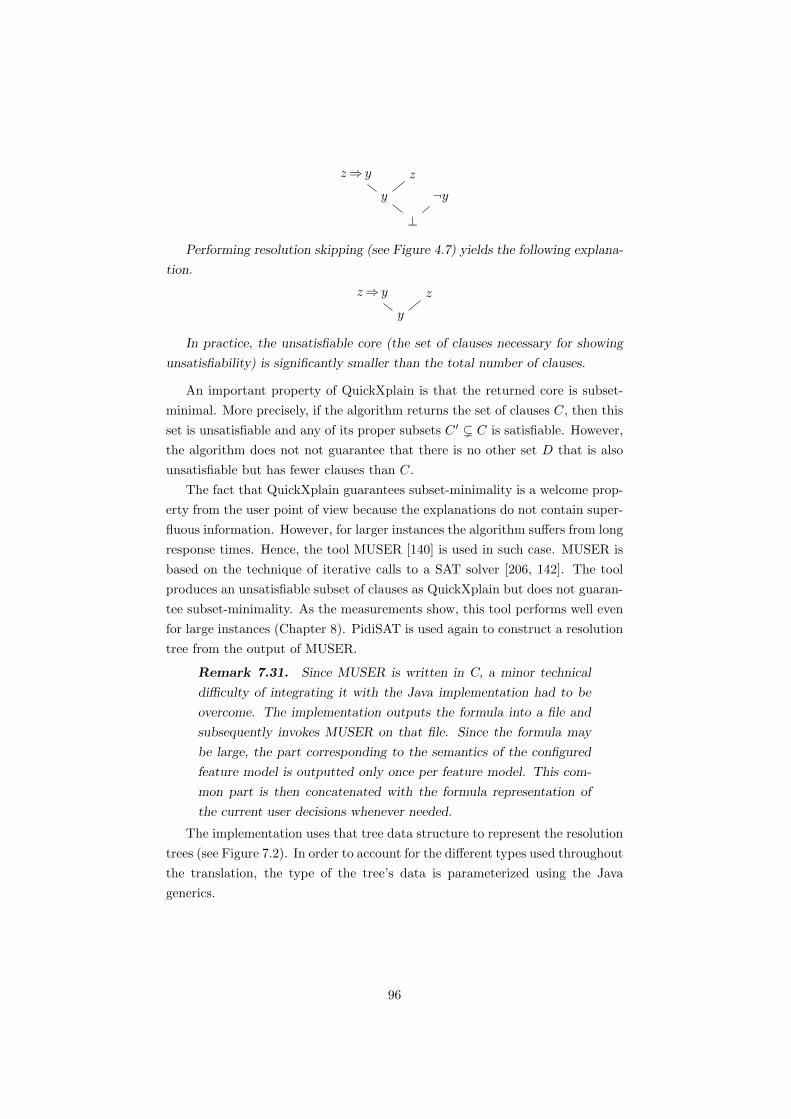
⊥
y
z⇒ y z
¬y
Performing resolution skipping (see Figure 4.7) yields the following explana-
tion.
y
z⇒ y z
In practice, the unsatisfiable core (the set of clauses necessary for showing
unsatisfiability) is significantly smaller than the total number of clauses.
An important property of QuickXplain is that the returned core is subset-
minimal. More precisely, if the algorithm returns the set of clauses C, then this
set is unsatisfiable and any of its proper subsets C ′ ( C is satisfiable. However,
the algorithm does not not guarantee that there is no other set D that is also
unsatisfiable but has fewer clauses than C.
The fact that QuickXplain guarantees subset-minimality is a welcome prop-
erty from the user point of view because the explanations do not contain super-
fluous information. However, for larger instances the algorithm suffers from long
response times. Hence, the tool MUSER [140] is used in such case. MUSER is
based on the technique of iterative calls to a SAT solver [206, 142]. The tool
produces an unsatisfiable subset of clauses as QuickXplain but does not guaran-
tee subset-minimality. As the measurements show, this tool performs well even
for large instances (Chapter 8). PidiSAT is used again to construct a resolution
tree from the output of MUSER.
Remark 7.31. Since MUSER is written in C, a minor technical
difficulty of integrating it with the Java implementation had to be
overcome. The implementation outputs the formula into a file and
subsequently invokes MUSER on that file. Since the formula may
be large, the part corresponding to the semantics of the configured
feature model is outputted only once per feature model. This com-
mon part is then concatenated with the formula representation of
the current user decisions whenever needed.
The implementation uses that tree data structure to represent the resolution
trees (see Figure 7.2). In order to account for the different types used throughout
the translation, the type of the tree’s data is parameterized using the Java
generics.
96
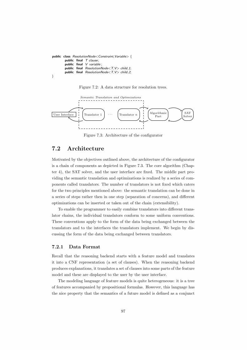
public class ResolutionNode<Constraint,Variable> {public final T clause ;public final V variable ;public final ResolutionNode<T,V> child 1;public final ResolutionNode<T,V> child 2;
}
Figure 7.2: A data structure for resolution trees.
User Interface Translator 1 . . . Translator nAlgorithmic
PartSAT
Solver
Semantic Translation and Optimizations
Figure 7.3: Architecture of the configurator
7.2 Architecture
Motivated by the objectives outlined above, the architecture of the configurator
is a chain of components as depicted in Figure 7.3. The core algorithm (Chap-
ter 4), the SAT solver, and the user interface are fixed. The middle part pro-
viding the semantic translation and optimizations is realized by a series of com-
ponents called translators. The number of translators is not fixed which caters
for the two principles mentioned above: the semantic translation can be done in
a series of steps rather then in one step (separation of concerns), and different
optimizations can be inserted or taken out of the chain (extensibility).
To enable the programmer to easily combine translators into different trans-
lator chains, the individual translators conform to some uniform conventions.
These conventions apply to the form of the data being exchanged between the
translators and to the interfaces the translators implement. We begin by dis-
cussing the form of the data being exchanged between translators.
7.2.1 Data Format
Recall that the reasoning backend starts with a feature model and translates
it into a CNF representation (a set of clauses). When the reasoning backend
produces explanations, it translates a set of clauses into some parts of the feature
model and these are displayed to the user by the user interface.
The modeling language of feature models is quite heterogeneous: it is a tree
of features accompanied by propositional formulas. However, this language has
the nice property that the semantics of a future model is defined as a conjunct
97

of the semantics of well defined parts of the model (Section 2.4.1). We call these
parts modeling primitives.
To achieve uniformity across formulas and feature models, we treat the mod-
els as flat structures—a set of modeling primitives. Table 7.1 lists the primitives
that are used in Lero S2T2 to describe feature models along with logic formula
corresponding to the semantics.
modeling primitive logic formulaRoot(r) vrOptionalChild(c, p) vc⇒ vpMandatoryChild(c, p) vc⇔ vpExcludes(a, b) ¬(va ∧ vb)Requires(a, b) va⇒ vbAlternativeGroup(p, {f1, . . . , fn}) (vf1 ∨ · · · ∨ vfn⇔ vp) ∧
∧i<j ¬(fi ∧ fj)
OrGroup(p, {f1, . . . , fn}) vf1 ∨ · · · ∨ vfn⇔ vfConstraint(φ) φSelectedFeature(f) vfEliminatedFeature(f) ¬vf
Table 7.1: Modeling primitives and their semantics
The names of the constructs closely follow the terminology used in the FODA
notation (Section 2.4.2). The primitive Root(r) determines that the feature r is
the root feature. The primitive OptionalChild(c, p) specifies that the feature c is
an optional child of the feature p. Analogously, MandatoryChild(c, p) is used for
mandatory children. The first argument to AlternativeGroup(p, {f1, . . . , fn})is a feature and the second is a set of features that form an alternative group of
the parent feature. The primitive OrGroup is used analogously. The primitive
Excludes(a, b) specifies that the features a and b are mutually exclusive and the
primitive Requires(a, b) specifies that the feature a requires the feature b. The
primitive Constraint(φ) is used for arbitrary propositional constraints.
The primitives SelectedFeature and EliminatedFeature stand out because
they are not part of the original FODA notation. The main purpose of these
primitives is to enable the user interface to specify user decisions by sending
these primitives to the backend. Making user decisions a part of the modeling
language has the following benefits. (1) It increases the homogeneity of the
communication: there is only one language of communication for specifying
both the initial feature model and for specifying user decisions. (2) It enables
storing intermediate stages of the configuration process as a set of primitives,
which is the same format as the format in which feature models are stored.
Decomposing the feature model into a set of primitives enables the reasoning
backend to focus on one primitive at a time. More importantly, the choice of
modeling primitives determines the granularity of explanations. Consider, for
98
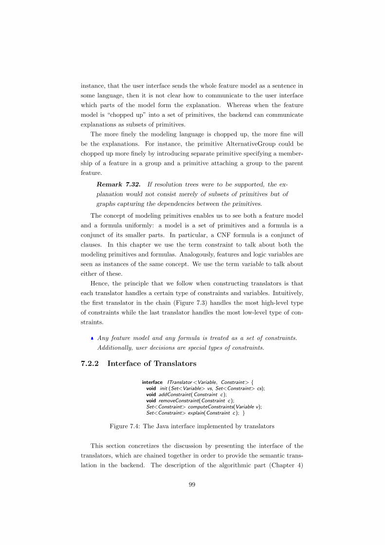
instance, that the user interface sends the whole feature model as a sentence in
some language, then it is not clear how to communicate to the user interface
which parts of the model form the explanation. Whereas when the feature
model is “chopped up” into a set of primitives, the backend can communicate
explanations as subsets of primitives.
The more finely the modeling language is chopped up, the more fine will
be the explanations. For instance, the primitive AlternativeGroup could be
chopped up more finely by introducing separate primitive specifying a member-
ship of a feature in a group and a primitive attaching a group to the parent
feature.
Remark 7.32. If resolution trees were to be supported, the ex-
planation would not consist merely of subsets of primitives but of
graphs capturing the dependencies between the primitives.
The concept of modeling primitives enables us to see both a feature model
and a formula uniformly: a model is a set of primitives and a formula is a
conjunct of its smaller parts. In particular, a CNF formula is a conjunct of
clauses. In this chapter we use the term constraint to talk about both the
modeling primitives and formulas. Analogously, features and logic variables are
seen as instances of the same concept. We use the term variable to talk about
either of these.
Hence, the principle that we follow when constructing translators is that
each translator handles a certain type of constraints and variables. Intuitively,
the first translator in the chain (Figure 7.3) handles the most high-level type
of constraints while the last translator handles the most low-level type of con-
straints.
Any feature model and any formula is treated as a set of constraints.
Additionally, user decisions are special types of constraints.
7.2.2 Interface of Translators
interface ITranslator<Variable, Constraint> {void init (Set<Variable> vs, Set<Constraint> cs);void addConstraint(Constraint c );void removeConstraint(Constraint c );Set<Constraint> computeConstraints(Variable v);Set<Constraint> explain(Constraint c ); }
Figure 7.4: The Java interface implemented by translators
This section concretizes the discussion by presenting the interface of the
translators, which are chained together in order to provide the semantic trans-
lation in the backend. The description of the algorithmic part (Chapter 4)
99

already specifies the set of messages exchanged between the configurator and
the user interface. This section discusses the same set of messages but at a more
technical level and accommodates for the fact that the feature model must be
translated into a CNF representation. Even though the current implementation
operates on feature models with propositional semantics, the interface of the
translators is designed in such way that the same interface can be used for more
complicated semantics in the future.
All the translators implement the same generic interface in order to maximize
uniformity over the translators. Additionally, the algorithmic part implements
this interface as well. Hence, the last translator does not need to be treated
specially since it connects to the algorithmic part as if it was another translator.
The motivation for this uniformity is that it enables each translator to rely
on the interface of the following translator (or the algorithmic part), rather than
on its concrete implementation. Consequently, this facilitates the a translator
can be removed or inserted into the chain as long as it fulfills the interface.
Each translator is parametrized by the type of constraints and variables that
it handles, e.g., the first translator handles feature modeling primitives and fea-
tures. For better intuition, one may think of each translator as of a configurator
for the pertaining type of constraints. Figure 7.4 presents a Java representation
of the interface where Java generics are used to capture the parametrization.
Let us discuss the individual methods.
The method init initializes a translator with a set of variables and constraints;
all constraints must constrain only the variables given here. The method init is
invoked just once—when the feature model is loaded. This method corresponds
to the message Init in Chapter 4.
Remark 7.33. The initialization phase fixes the set of considered
variables. Nevertheless, it might be useful to have means for manip-
ulating the set of variables on the fly.
The purpose of the methods addConstraint and removeConstraint is to add
and retract user decisions, respectively. The method removeConstraint must not
be invoked on a constraint given via the init method. These methods generalize
the messages assert and retract in Chapter 4. When the user selects or
eliminates a feature, the user interface sends the appropriate primitive as a
parameter of the method addConstraint of the first translator. However, the
signature of the methods enables a translator to support more general decisions
such as “feature x or y must be selected”.
The function computeConstraints(Variable v) infers constraints for the given
variable. This method generalizes the messages Lock and Unlock in Chap-
ter 4. If this method returns the empty set, the variable is not constrained,
100

i.e., the variable is unlocked. To signal that a variable is locked, the translator
returns a set containing the appropriate constraint. For instance, in the case
of feature models, to signal that a feature is locked is signaled by sending a set
containing either the primitive SelectFeature or EliminateFeature. In the case
of CNF, locking is achieved by sending the corresponding literal.
Clearly, this mechanism is more flexible than just the two messages Lock
and Unlock. If one would want to express, for example, that a certain number
must be within a certain range, then it would suffice to extend the type of
constraints with such constraint.
Note that in Chapter 4, the configurator infers constraints for all the vari-
ables after each user action. In this respect, the function computeConstraints
corresponds to the body of the loop in Test-Vars (Figure 4.3). Each of these
iterations determines whether the inspected variable is bound or not. The rea-
son why the interface provides the function computeConstraints separately is
that it enables the user interface to inspect only certain variables. This can be
used to improve the efficiency—if some portions of the model are not displayed,
it is not necessary to query them.
The function explain(Constraint c) provides an explanation for a given
constraint c. The constraint c must have been previously returned by
computeConstraints. The method must guarantee that the returned explana-
tion contains only such constraints that were added via init or addConstraint
and not removed in the meantime. This method corresponds to the message
Explain in Chapter 4.
Because the translators are directly implemented in Java, it is hard to cap-
ture in the interface that the translator is expected to be connected to the
translator that follows in the translator-chain (Figure 7.3). The convention
used in the implementation is that the following translator is specified in the
constructor of each translator. Hence, each translator has a constructor of the
form Translator(ITranslator<CT,VT> followingTranslator).
A specific chain of translators is then constructed by nested constructor
calls where the algorithmic part is constructed first, i.e., the chain of translators
T1,. . . ,TN followed by the algorithmic part A is constructed by the Java code:
new T1(new T2(... new TN(new A())...)).
Remark 7.34. The convention just outlined could be resolved more
elegantly if the configurator was implemented in the context of some
middleware that would enable modeling the conventions explicitly
by a software architecture description language [146].
101
All translators implement an instantiation of the same generic interface.
This enables constructing different translator chains which are checked
by the Java type system.
7.3 Implementation
This section describes the implementation of the backend in Lero S2T2. It is not
the objective of this section to describe the actual Java code but to highlight
the main characteristics of the implementation. The description begins with the
different types of constraints used in the backend.
7.3.1 Constraint Types
Each translator implements the interface discussed above (see Figure 7.4) and
translates between two types of constraints: certain type of constraints are
sent to the translator through the methods of the interface and certain type of
constraints is obtained from the translator that follows in the chain.
Constraint types are represented as is common in object oriented program-
ming. Each constraint type corresponds to a Java class whose member fields
determine the pertaining variables. To represent a family of constraint types,
the classes inherit from a class representing that particular family. For instance,
the primitive SelectFeature is represented as a class with a member field speci-
fying the selected feature. Since SelectFeature belongs into the family of feature
model primitives, it inherits from a class representing the family of feature model
primitives (in the following text this class is denoted as FMP).
The implemented families of constraints are listed in Table 7.2. The table
contains a brief description of each of these families and a description of the
constraint and the variable type that are used to instantiate the ITranslator
interface (Figure 7.4).
Name Description ConstraintType
VariableType
FMP feature models feature modelprimitive
feature
EPL extended propositionallogic
extended for-mula
variable
PL propositional logic formula variableCNF conjunctive normal
formclause variable
Table 7.2: Constraint families
The family FMP contains the feature primitives presented above (see Ta-
ble 7.1). The family EPL contains standard logic connectives but additionally
102

User Interface FMP2EPL EPL2PL PL2CNF BISAlgorithmic
Part
Figure 7.5: Concrete architecture of the configurator
contains the construct select(p, v1, ..., vN) specifying that exactly one of
the v1, ..., vN must be True iff p is True. This construct is used in the
translation of the semantics of alternative groups. The reason to have a special
construct for this is that translating it into standard logic connectives can be
done in multiple ways[11, 184, 62, 137]. The family PL is a standard proposi-
tional logic without the construct select. Finally, the family CNF is used to
capture a formula in the conjunctive normal form.
The task of the translators is to provide a gradual translation from the family
FMP to the family CNF. This is discussed in the following section.
7.3.2 Implementation of Translators
Figure 7.5 shows the translators that provide the semantic translation in
Lero S2T2. The translator FMP2EPL translates from feature primitives to propo-
sitional logic while using the construct select. The translator EPL2PL desugars
this construct leaving only the standard connectives. The translator PL2CNF
translates propositional logic into the conjunctive normal form; the current im-
plementation is using de Morgan’s laws and therefore does not add any new
variables (see Section 2.1.3).
These translators enable us to construct a chain from feature model prim-
itives to conjunctive normal form. Additionally, there is the translator BIS
implementing the BIS-optimization (see Chapter 5). Recall that the optimiza-
tion expects conjunctive normal form and produces conjunctive normal form.
Therefore, this translator handles the constraint family CNF and is connected
just after the translator PL2CNF. Thanks to the modularization principles used
in the design, the translator BIS can be taken out of the chain so that the
translator PL2CNF is connected directly to the algorithmic part.
Remark 7.35. Observe that the translator BIS expects the same
type of constraint from the translator on its left and from the trans-
lator on its right. This is in fact a necessary condition for a translator
to be freely removable from the chain.
All of the translators work in a similar fashion. Each of the translators
maintains a mapping between the two pertaining constraint types and a mapping
between the two types of variables. These mappings are initialized in the method
init and are updated in the method addConstraint. The other methods of the
103
interface use these mappings to convert between the two types.
As an example, let us look on the implementation of the translator
FMP2EPL— from feature model primitives to extended propositional logic. This
translator implements the interface ITranslator with the family FMP. The con-
structor of the translator expects a reference to the translator that follows in
the chain and implements the interface ITranslator instantiated with the con-
straint family EPL. The translator FMP2EPL maintains a one-to-many mapping
from feature model primitives to formulas and a one-to-one mapping from fea-
tures to variables.
The method init populates these mappings with the initial set of primitives
and the corresponding semantics expressed as the extended propositional logic
formulas.
The method addConstraint(FeatureModelPrimitive p) expects one of the prim-
itives SelectFeature and EliminateFeature; it translates the primitive into the
corresponding literal l and adds the correspondence between the primitive and
the literal into the mapping. Finally, it calls the method addConstraint of the
following translator with l as the argument.
The method removeConstraint(FeatureModelPrimitive p) removes the
primitive p from the mapping and calls the method removeConstraint in the
following translator for all those extended propositional logic formulas that are
not mapped to. The reason why the method cannot simply remove all the
formulas that correspond to the semantics of the primitive p is that the mapping
is not necessarily injective.
The method computeConstraints(Feature f) looks up in the variable
mapping the variable corresponding to the feature f and calls the method
computeConstraints(Variable v) of the following translator. This method
either returns the empty set (if the variable is unbound) or a set containing
the bound literal. If the following translator returns the empty set, then the
methods returns the empty set since the feature is not bound. If the follow-
ing translator returns a bound literal, the method converts the literal to the
appropriate primitive and returns a singleton set containing that primitive.
The implementation of the method explain(FeatureModelPrimitive p) first
calls the method explain of the following translator for each formula correspond-
ing to the semantics of the primitive p. Then it computes the union of these
formulas and converts them back to a set of primitives using the inverse of the
mapping between primitives and formulas.
The other translators are implemented analogously. However, there are some
differences in terms of the cardinalities of the mappings. For instance, the trans-
lator BIS maintains a many-to-one mapping between variables since variables
in the same BIS are represented by a single variable (see Chapter 5) while the
104

other translators maintain a one-to-one mapping between variables. For more
details see the source code1.
7.4 Summary of the Design
This chapter has presented the design of the reasoning backend used in the con-
figurator Lero S2T2. The architecture of the backend resembles the well-known
architecture pipe-and-filter. However, compared to the traditional setting, the
components in the chain communicate in both directions since the backend needs
to provide explanations.
All the information exchanged between the components is represented as
sets of constraints. The type of these constraints depends on the phase of the
semantic translation. As is common, the translation starts from the most high-
level type of constraints and proceeds to the most low-level type of constraints.
In some sense, this follows the well-known pattern of step-wise refinement [200,
57, 18, 17].
If the feature model is to be treated as a set of constraints, it needs to be
chopped up into a set of primitives. Even that is not all that novel. Indeed,
the primitives used to describe feature models correspond to relations in the
entity-relation modeling, such as UML. Hence, it is possible to assume that this
approach to capturing feature models could be generalized to other models as
well.
The components comprising the implementation are components in the ob-
ject oriented sense, i.e., the implementation of the translators are separate
classes that communicate with each other through an interface. This interface
is prescribed by a generic interface which is instantiated by the specific type
of constraints that the given translator handles. An alternative to this setup
would be cross-cutting components used in feature oriented or aspect oriented
programming. In such setup there would be a single class providing the seman-
tic translation. This class would be modified by different features (or aspects)
providing the functionality of different translation phases.
The disadvantage of components organized in the object oriented sense is
efficiency. Each of the translators needs to maintain a mapping between the
two pertaining types of constraints. Whenever a translator responds to some
user action, it needs to perform a look-up in these mappings. The advantage
of this approach is that the programmer that is adding new translators, or is
composing some existing ones, can treat the translators as black-boxes. If the
translation where organized in cross-cutting components, this additional book-
1http://kind.ucd.ie/products/opensource/Config/releases/
105

keeping could be eliminated. Nevertheless, at the price of making the code more
entangled and hampering extensibility. However, the look-up routines did not
come up as problematic during the profiling of the implementation.
This particular design has proven to be useful throughout the development
of Lero S2T2. According to our experience, the activities that benefit the most
from this design are experimentation and evolution as a new type of functionality
can be implemented as a separate translator and this translator is inserted into
the chain only by the programmer who is testing it.
In summary, the contributions of this chapter are: a description how to
implement a configurator in an object oriented language and a technological
solution for providing explanations when using a SAT solver that does not return
resolution trees.
106

Chapter 8
Empirical Evaluation
This chapter presents a number of measurements performed using the described
implementation of the configurator run on third party instances. The motiva-
tion for these measurements is twofold. Firstly, the measurements should show
whether the described algorithms are suitable for the interactive setting or not.
In particular, whether the response time is acceptable for a human. Secondly,
the measurements should show the impact of the proposed optimizations.
Section 8.1 describes the testing environment and process. Section 8.2 de-
scribes the test data and their main characteristics. Section 8.3 presents mea-
surements that were done for the response time of the algorithm computing
bound variables during an interactive configuration process. This response time
determines how long the user has to wait before getting a response from the
configurator after he or she made a decision. The effect of the BIS-optimization
(Chapter 5) is also studied. Section 8.4 studies how many times the SAT solver
was invoked when computing bound variables. Section 8.5 studies the explana-
tion sizes and Section 8.6 studies the explanation response times. Section 8.7
presents measurements that were done for the technique of computing dispens-
able variables. Two aspects of this technique are studied: the response time and
the effectiveness. Section 8.8 evaluates whether the number of measurements
gives us a good estimate of the overall behavior of the configurator using the
method of confidence intervals. Section 8.9 compares different types of expla-
nations and argues that explanations based on resolution trees (Section 4.5) are
more informative than explanations highlighting only pertaining user decisions.
Finally, Section 8.10 draws conclusions from the measurement and summarizes
the results.
The measurements in this chapter are presented in the form of histograms,
i.e., the horizontal axis corresponds to the value being observed and the ver-
tical axis is the number of times that particular value occurred in the set of
107
observations in questions (frequency).
8.1 Testing Environment and Process
The measurements were performed on nine machines where each has Quad-
Core AMD Opterontm 64-bit processors with 512 kB cache. Eight out of these
nine machines have 8 processors while one of these machines has 16 processors.
However, since no multithreading was used this does not affect the performance.
The installation of the Java virtual machine (Java HotSpottm 64-Bit Server VM)
was identical on all the machines and its heap size was limited to 2 GB for each
measurement.
All the measurements were performed in the following three phases.
• Test generation—in this phase testing data were generated and recorded in
a dedicated format. In particular, the testing data were sequences of user
decisions recorded as a file whose each line recorded which user decision
was made (selection or elimination of a variable).
• Test execution—in this phase the data generated in the previous phase
were read in and executed while recording the data to be collected (re-
sponse times, etc.). It should be noted that all the times are stopwatch
times, i.e., obtained by subtracting the time observed before the measured
operation from the time observed after the operation.
• Data aggregation—using custom scripts and small Java programs the
times were aggregated to obtain average values and data for the plots.
The plots were rendered using the program gnuplot [82].
8.2 Test Data
Seven instances were chosen to perform the evaluation. Three of these instances
are large feature models with up to hundreds of features, available at the feature
model repository [66]: E-shop, Violet, and Berkeley. A toy example representing
a feature model of a T-shirt was added as this example commonly occurs in
articles on configuration. The largest instance evaluated is the Linux kernel
variability model [22].
Two instances are not feature models but randomly-chosen DIMACS format
(Center for Discrete Mathematics and Theoretical Computer Science format)
examples used in SAT competitions and benchmarking: 3blocks and rocket. In
the following text we refer to the feature models and the Linux kernel instance
108
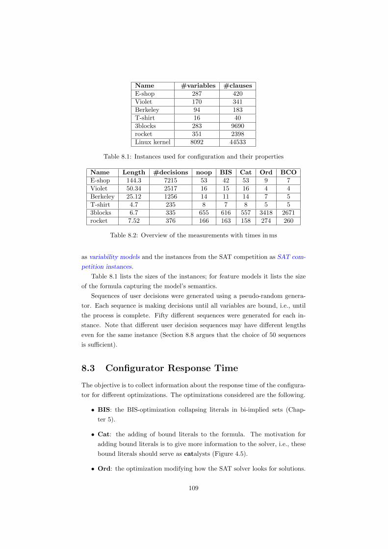
Name #variables #clausesE-shop 287 420Violet 170 341Berkeley 94 183T-shirt 16 403blocks 283 9690rocket 351 2398Linux kernel 8092 44533
Table 8.1: Instances used for configuration and their properties
Name Length #decisions noop BIS Cat Ord BCOE-shop 144.3 7215 53 42 53 9 7Violet 50.34 2517 16 15 16 4 4Berkeley 25.12 1256 14 11 14 7 5T-shirt 4.7 235 8 7 8 5 53blocks 6.7 335 655 616 557 3418 2671rocket 7.52 376 166 163 158 274 260
Table 8.2: Overview of the measurements with times in ms
as variability models and the instances from the SAT competition as SAT com-
petition instances.
Table 8.1 lists the sizes of the instances; for feature models it lists the size
of the formula capturing the model’s semantics.
Sequences of user decisions were generated using a pseudo-random genera-
tor. Each sequence is making decisions until all variables are bound, i.e., until
the process is complete. Fifty different sequences were generated for each in-
stance. Note that different user decision sequences may have different lengths
even for the same instance (Section 8.8 argues that the choice of 50 sequences
is sufficient).
8.3 Configurator Response Time
The objective is to collect information about the response time of the configura-
tor for different optimizations. The optimizations considered are the following.
• BIS: the BIS-optimization collapsing literals in bi-implied sets (Chap-
ter 5).
• Cat: the adding of bound literals to the formula. The motivation for
adding bound literals is to give more information to the solver, i.e., these
bound literals should serve as catalysts (Figure 4.5).
• Ord: the optimization modifying how the SAT solver looks for solutions.
109

Frequ
ency
0
1000
2000
3000
4000
5000
6000
7000
8000
0 30 60 90 120 150 180 210 240 270 300 330
response time for Eshop-fm.xml
nooptBISCatOrd
BCO
Time (ms)
Figure 8.1: Distribution of response times for E-shop
In particular this optimization changes the ordering of the search space
traversal (Section 4.4).
The measurements were carried out with five different combinations of the
optimizations. One version, denoted as noopt, does not use any of these opti-
mizations. Another three versions use one of these optimizations. And, the last
version, denoted as BCO, uses all of them.
For each optimization combination, instance, and user decision sequence the
measurement was repeated ten times and averaged to filter out noise caused by
the operating system and the machine1.
Table 8.2 summarizes the results of the measurements. The first column is
the name of the investigated instance. The second column is the average length
of a user decision sequence; observe that this is in fact 50 times the first column
since 50 sequences were evaluated for each instance. The third column is the
total number of user decisions over all sequences. Each of the last five columns
shows the average over all user decisions and sequences for one of the version of
optimizations in milliseconds.
Figures 8.1–8.6 present the different time distributions for different instances
and optimization combinations, except for the Linux kernel instance. The hor-
izontal axis is the response time and vertical corresponds to the number of
1The solver has a random component but this is initialized by a constant seed and thereforeis not observable in repeated measurements.
110

Frequ
ency
0
500
1000
1500
2000
2500
0 20 40 60 80 100 120 140
response time for violet_model.m
nooptBISCatOrd
BCO
Time (ms)
Figure 8.2: Distribution of response times for Violet
Frequ
ency
0
200
400
600
800
1000
1200
0 15 30 45 60 75 90 105 120 135
response time for berkeley.m
nooptBISCatOrd
BCO
Time (ms)
Figure 8.3: Distribution of response times for Berkeley
111
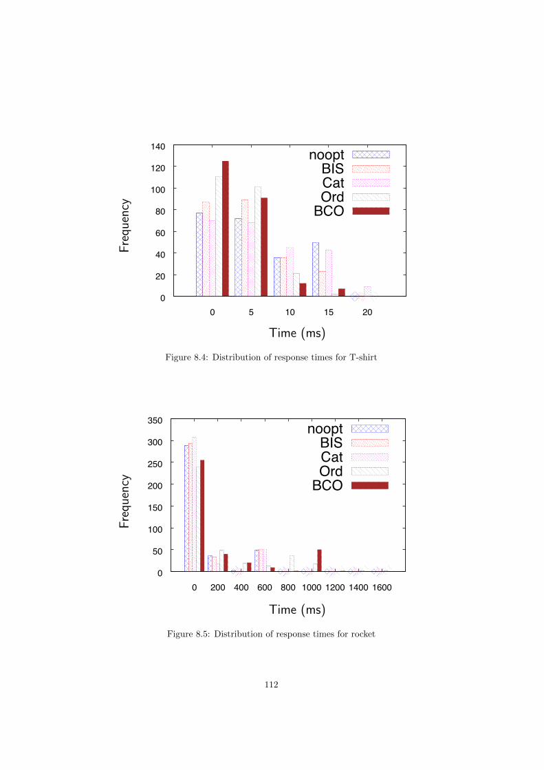
Frequ
ency
0
20
40
60
80
100
120
140
0 5 10 15 20
response time for TShirt.m
nooptBISCatOrd
BCO
Time (ms)
Figure 8.4: Distribution of response times for T-shirt
Frequ
ency
0
50
100
150
200
250
300
350
0 200 400 600 800 1000 1200 1400 1600
response time for sat_rocket_ext.b.cnf
nooptBISCatOrd
BCO
Time (ms)
Figure 8.5: Distribution of response times for rocket
112

Frequ
ency
0
50
100
150
200
250
300
0 1s 2s 3s 4s 5s 6s 7s 8s 9s 10s 11s 12s 13s 14s 15s 16s
response time for 3blocks.cnf
nooptBISCatOrd
BCO
Time (s)
Figure 8.6: Distribution of response times for 3blocks
occurrences of the response time. All the times are in milliseconds except for
the diagram concerning the instances 3blocks. The response times are clustered
to obtain a histogram. For instance, in the E-shop distribution there are over
7000 occurrences of response times below 30 ms for the BCO optimization com-
bination. Since 7215 cases were evaluated for the E-shop instance, over 97% of
these cases were below 30 ms using the BCO optimization combination.
Linux Kernel Instance Since the Linux kernel instance is substantially
larger than the other instances, only one iteration for each user decision se-
quence was performed as otherwise the measurements would require a couple
of months. However, Section 8.8 shows that the variations over different itera-
tions and sequences are small, which suggests that the performed measurements
provide a good estimate of the overall behavior.
Another issue was with evaluating the instance without the ord heuristic.
The response times were significantly worse without the heuristic—around 1
minute per user decision. Hence performing a precise evaluation without the
heuristic is not possible within a practical time frame.
The Linux kernel instance yielded the following observations. The average
length of a user decision sequence was 4195.28, i.e., the total number of observed
cases was 209764.
The evaluated optimization combinations are the following O—ord op-
timization, BO—ord optimization coupled with the BIS-optimization, and
BrO—ord optimization coupled with the BIS-optimization that is not using
113
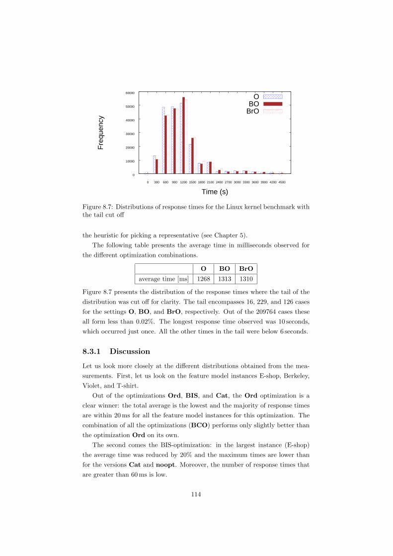
0
10000
20000
30000
40000
50000
60000
0 300 600 900 1200 1500 1800 2100 2400 2700 3000 3300 3600 3900 4200 4500
Fre
quen
cy
Time (s)
OBO
BrO
Figure 8.7: Distributions of response times for the Linux kernel benchmark withthe tail cut off
the heuristic for picking a representative (see Chapter 5).
The following table presents the average time in milliseconds observed for
the different optimization combinations.
O BO BrO
average time [ms] 1268 1313 1310
Figure 8.7 presents the distribution of the response times where the tail of the
distribution was cut off for clarity. The tail encompasses 16, 229, and 126 cases
for the settings O, BO, and BrO, respectively. Out of the 209764 cases these
all form less than 0.02%. The longest response time observed was 10 seconds,
which occurred just once. All the other times in the tail were below 6 seconds.
8.3.1 Discussion
Let us look more closely at the different distributions obtained from the mea-
surements. First, let us look on the feature model instances E-shop, Berkeley,
Violet, and T-shirt.
Out of the optimizations Ord, BIS, and Cat, the Ord optimization is a
clear winner: the total average is the lowest and the majority of response times
are within 20 ms for all the feature model instances for this optimization. The
combination of all the optimizations (BCO) performs only slightly better than
the optimization Ord on its own.
The second comes the BIS-optimization: in the largest instance (E-shop)
the average time was reduced by 20% and the maximum times are lower than
for the versions Cat and noopt. Moreover, the number of response times that
are greater than 60 ms is low.
114

The optimization Cat does not seem to be very helpful. For some instances
it even adds a tail to the distribution.
Now let us look at the Linux kernel instance. Clearly, the Ord was greatly
important since it wasn’t possible to evaluate the instance without it. The BIS-
optimization did not prove to be useful for the instance. In fact, the optimization
slightly worsens the response times. However, this worsening changes the av-
erage response time by only a few milliseconds. This is most likely due to the
fact that there are few BISs (strongly connected components in the implication
graph) in the instance.
Most of the response times are around 1 second (see Figure 8.7). The times
around 2 seconds appear in ca. thousand cases, which is 0.5% of the total number
of cases. The distribution has a very long tail, meaning that the user will have
to wait up to 10 seconds in some instances. However, these cases are very rare.
In particular, the response time of 10 seconds occurred just once.
The numbers are very different for the instances coming from SAT compe-
titions (3blocks and rocket). The configurator performs much worse with the
optimization Ord than without it. That is already obvious from the averages
(the average increased six times for 3blocks). The explanation for this phe-
nomenon is that these instances are more difficult for the SAT solver and the
Ord heuristics takes away some smartness from the solver. In the case of the
feature model instances taking away the smartness makes up for the fact that
the satisfiability tests find more quickly the literals that are not bound.
The BIS optimization is only moderately successful on these instances. How-
ever, the combination of the optimizations mitigates the worsening in times
caused by the Ord optimization.
A difference between the feature model instances and the SAT instances can
also be seen in Table 8.2. Both of the SAT instances have more variables than
the feature model instances but a configuration process on the SAT instances is
shorter. This indicates tighter dependencies between the variables: a small set
of decisions determines values for all the other variables.
An interesting phenomenon is that all the distributions have long tails, i.e.,
there are many short times. This is explained by the fact that as a configuration
process progresses, the instance is getting more constrained by the user decisions
made so far. Effectively, the satisfiability tests are becoming easier. The fact
that there are so many short times, signifies that these tests become fast only
after a few decisions.
Remark 8.36. To analyzed in more detail the bad times, one could
analyze only some prefixes of the user decision sequences. However,
it is not clear how this cut off point should be chosen.
115
The optimization Ord is highly efficient for loosely constraint instances.
the optimization BIS yields only moderate speedups but does so for all
the instances.
8.4 Number of Calls to The Solver
In Chapter 4 we show that the solver is called at most n+1 times after each user
decision, where n is the number of variables (Claim 3). However, we hypothesize
that the number of calls is in practice significantly lower (see also Remark 4.13).
This section presents the number of calls to the solver observed in the evaluated
benchmarks. Even though n+1 is the maximal number off calls, for the purpose
of the following calculations we assume it is n since the SAT solver is called
once when the configurator is initialized in order to test that the given instance
has at least one valid configuration (the theoretical part considers this to be a
precondition).
Even though the number of variables is constant throughout the configura-
tion process, the instance becomes easier throughout the process as the user
is making decisions. Hence, the number of calls the solver is interesting with
respect to the number of variables whose values are not determined by a user
decision.
Figures 8.8–8.13 show distributions of percentages calculated as 100 ∗ c/f ,
where f is the number of variables whose values are not determined by user
decisions and c is the number of calls the solver. These measurements were
performed over the same set of sequences of user decisions as the measurements
for response times.
The Linux kernel benchmark is not plotted as the numbers of calls to the
solver are predominantly smaller than the number of variables not decided by
the user. This is due to the fact that the instance was evaluated only with the
optimizations containing the ord heuristic. Out of the 209764 cases, the solver
was called less than 10 times in 90% cases. The maximum number of calls the
solver observed was 725, which occurred only once.
8.4.1 Discussion
As expected, the optimization Ord dramatically decreases the number of calls
to the solver. With this optimization, most of the times the solver needs to be
called only 10%-times with respect to the number of variables not decided by
the user. In the Linux kernel instance the number of calls to the solver was
almost constant ranging between 0–10 calls the solver in 90% of the cases. A
few cases occurred where the solver needed to be called a few hundred times.
help these cases, however, where extremely rare.
116

Frequ
ency
0
1000
2000
3000
4000
5000
6000
7000
8000
0 10 20 30 40 50 60
nooptBISCatOrd
BCO
Percentege of SAT calls
Figure 8.8: Percentages of number of calls to the solver for E-shop
Frequ
ency
0
500
1000
1500
2000
2500
0 10 20 30 40 50 60 70 80 90
nooptBISCatOrd
BCO
Percentege of SAT calls
Figure 8.9: Percentages of number of calls to the solver for Violet
117

Frequ
ency
0
200
400
600
800
1000
1200
0 10 20 30 40 50 60 70 80 90
nooptBISCatOrd
BCO
Percentege of SAT calls
Figure 8.10: Percentages of number of calls to the solver for Berkeley
Frequ
ency
0
10
20
30
40
50
60
70
80
0 5 10 15 20 25 30 35 40 45 50 55 60 65 70 75 80 85 90
nooptBISCatOrd
BCO
Percentege of SAT calls
Figure 8.11: Percentages of number of calls to the solver for T-shirt
118

Frequ
ency
0
20
40
60
80
100
120
140
160
180
0 10 20 30 40 50 60
nooptBISCatOrd
BCO
Percentege of SAT calls
Figure 8.12: Percentages of number of calls to the solver for 3blocks
Frequ
ency
0
50
100
150
200
250
0 10 20 30 40 50
nooptBISCatOrd
BCO
Percentege of SAT calls
Figure 8.13: Percentages of number of calls to the solver for rocket
119

The distributions for the other optimizations (noop, BIS, and Cat) ex-
hibit only minor differences from one another, with the exception of the T-shirt
instance. Interestingly, the structure of these distributions varies significantly
across the benchmarks. In the E-shop instance the distributions peak at 40%
and quickly drops to 0 at 60%. In the Violet instance, the distributions slowly
ascend to the peak at 40% and drop to 0 at 70%. In the Berkeley instance,
the distributions peak at 20% and drop to 0 at 50%. The distributions of the
T-shirt instance are somewhat erratic, which most likely is due to the small size
of the instance.
Both of the SAT competition instances yield similar distributions. Each
peaks 10% and descends quickly to 0. An interesting phenomenon appears in
the 3blocks instance, where ca. 50 cases needed 60% invocations of the solver for
all the optimizations. This is most likely due to situations where many variables
are bound and therefore the Ord heuristic does not have a great effect.
In summary, the Ord heuristic decreases the number of calls the solver
significantly. If the heuristic is not used, the expected number of calls to the
solver is in the range of 20%–40% of the number of variables not decided by the
user.
8.5 Explanation Sizes
In this section we overview of the evaluation of the explanation sizes. Two
different mechanisms were used to produce explanations. One mechanism was
QuickXplain [111], which guarantees subset-minimality but does not scale well.
The second mechanism was the tool MUSER [140]. Both of these mechanisms
were used with the combination of an additional SAT solver for constructing
resolution trees from unsatisfiable cores (for details on how these tools are inte-
grated into the explanation mechanism see Section 7.1).
MUSER was used for larger instances (SAT competition and Linux kernel).
The rest of the instances were evaluated with QuickXplain. It was not possible
to evaluate the 3blocks benchmark because the observed proofs were too large
(over 231), which caused unwieldy response times.
Figure 8.14 summarizes which techniques were used for the individual in-
stances.
What is in particular interest for us is the effect of the BIS-optimization
on explanations’ size. Recall that the BIS-optimization partitions the set of
literals into sets of equivalent literals in order to reduce the number of queries
to the solver. Each set of equivalent literals is represented by one literal—the
representative.
120

Name Explanation mechanismE-shop QuickXplainViolet QuickXplain
Berkeley QuickXplainT-shirt QuickXplain
Linux-kernel MUSERrocket MUSER3blocks not evaluated
Figure 8.14: Techniques used for explanations (see Section 7.1 for implementa-tion details)
We show how to reconstruct resolution trees obtained on the optimized for-
mula and we show that the choice of representatives influences the size of the
reconstructed proof. Further, we devise a heuristic that picks such representa-
tives that are likely to yield smaller reconstructed proofs (Section 5.2).
To evaluate the effectiveness of this heuristic, the reconstruction was once
done with a randomly picked representatives and once with representatives
picked according to this heuristic.
Hence, the following settings were evaluated: no optimization (noop), BIS-
optimization (BIS), and BIS-optimization with random representative (BIS-
RR). The following table presents the average sizes of the observed explanations.
Name noop BIS BIS-RR
E-shop 8 7 15
Violet 4 4 4
Berkeley 8 10 15
T-shirt 5 6 10
Linux-kernel 15 16 16
rocket 6,001,001 3,519,066 6,153,248
3blocks n/a n/a n/a
Figures 8.15—8.19 depict the distributions of explanation sizes for the indi-
vidual instances. The distribution for the rocket instance is not plotted due to
its unusual structure. Out of the 349 measured cases 124 cases yield explana-
tions of size smaller than 100. The rest of the cases are evenly split up to the
maximum size, where the maximum size was 4.6 ∗ 108 for noop, 1.6 ∗ 108 for
BIS, and 1.7 ∗ 109 for BIS-RR.
8.5.1 Discussion
The explanation sizes for the variability models are small. Even for the Linux
kernel instance the average size is 16, which is well-manageable for a user. How-
121
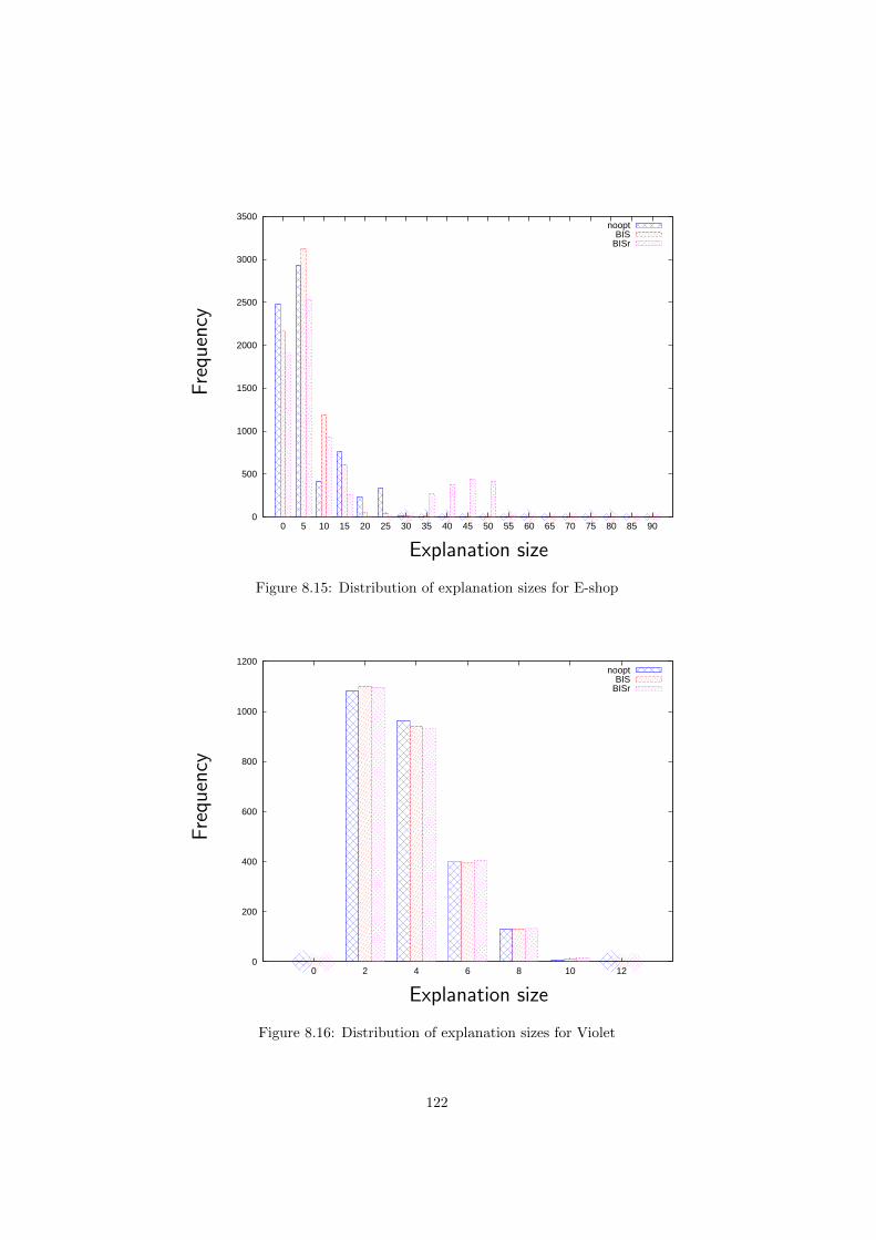
Frequ
ency
0
500
1000
1500
2000
2500
3000
3500
0 5 10 15 20 25 30 35 40 45 50 55 60 65 70 75 80 85 90
nooptBIS
BISr
Explanation size
Figure 8.15: Distribution of explanation sizes for E-shop
Frequ
ency
0
200
400
600
800
1000
1200
0 2 4 6 8 10 12
nooptBIS
BISr
Explanation size
Figure 8.16: Distribution of explanation sizes for Violet
122

Frequ
ency
0
200
400
600
800
1000
1200
0 5 10 15 20 25 30 35 40 45
nooptBIS
BISr
Explanation size
Figure 8.17: Distribution of explanation sizes for Berkeley
Frequ
ency
0
50
100
150
200
250
300
350
400
450
0 4 8 12 16 20 24 28 32 36 40
nooptBIS
BISr
Explanation size
Figure 8.18: Distribution of explanation sizes for T-shirt
123

Frequ
ency
0
10000
20000
30000
40000
50000
60000
0 5 10 15 20 25 30 35 40 45 50 55 60 65 70 75 80 85 90 95 100
nooptBIS
BIS-RR
Explanation size
Figure 8.19: Distribution of explanation sizes for Linux kernel
ever, for the instances from the SAT competition the obtained explanations
turned out to be unwieldy.
The heuristic used in BIS-optimization for choosing representatives proven
to be important. For instance, in the E-shop instance not using the heuristic
doubles the average explanation size and significantly prolongs the tail of the
distribution.
Now let us look at the comparison of sizes of explanations constructed with-
out the BIS-optimization and the sizes constructed in the presence of the heuris-
tic. As expected, in most cases the reconstruction of the proof yields bigger
proofs than those obtained without the optimization. However, this increase in
size is relatively small. The explanation average grew by 1 in Linux kernel and
T-shirt, it grew by 2 for Berkeley, and it didn’t change for Violet.
Interestingly, the reconstructed explanations’ sizes are smaller for the E-
shop and rocket instances. Most likely, the reason for that is that the algorithm
computing the unsatisfiable core (QuickXplain or MUSER) is operating on a
smaller formula and therefore is capable of finding smaller cores.
In summary, the explanation sizes are small for variability models but tend
to grow rapidly for complex formulas. The proposed heuristic for choosing a
representative in the BIS-optimization is important for the explanations’ size,
and, in some cases the reconstructed proof can be smaller than a proof obtained
from the unoptimized formula (E-shop and rocket).
124

Name noop BIS Cat Ord BCOE-shop 94 53 94 99 36Violet 20 21 22 28 23Berkeley 15 9 14 19 12T-shirt 20 11 19 14 11rocket 327 157 139 144 143
Name O BO BrOLinux kernel 465 469 555
Table 8.3: Average explanation response times in ms
Frequ
ency
0
20
40
60
80
100
120
0 100 200 300 400 500
nooptBISCatOrd
BCO
Explanation time (s)
Figure 8.20: Distribution of explanation times for E-shop
8.6 Explanation Times
This section provides an overview of the observed response times for computing
explanations. Table 8.3 presents the average response time for the individual
instances and optimization combinations. Figures 8.20—8.25 depict the distri-
butions of the times needed to compute explanations.
8.6.1 Discussion
The explanation response times are overall satisfactory. Even for the Linux
kernel instance the average response times are predominantly around 0.5 ms.
Somewhat surprising is the fact that the response times for the rocket instance
125

Frequ
ency
0
5
10
15
20
25
0 20 40 60 80 100 120 140 160
nooptBISCatOrd
BCO
Explanation time (s)
Figure 8.21: Distribution of explanation times for Violet
Frequ
ency
0
5
10
15
20
25
30
35
40
0 10 20 30 40 50 60 70 80 90 100 110 120 130 140 150 160 170
nooptBISCatOrd
BCO
Explanation time (s)
Figure 8.22: Distribution of explanation times for Berkeley
126

Frequ
ency
0
1
2
3
4
5
6
7
0 10 20 30 40
nooptBISCatOrd
BCO
Explanation time (s)
Figure 8.23: Distribution of explanation times for T-shirt
Frequ
ency
0
50
100
150
200
250
300
350
0 200 400 600 800 1000 1200 1400 1600 1800 2000 2200 2400
nooptBISCatOrd
BCO
Explanation time (s)
Figure 8.24: Distribution of explanation times for rocket
127
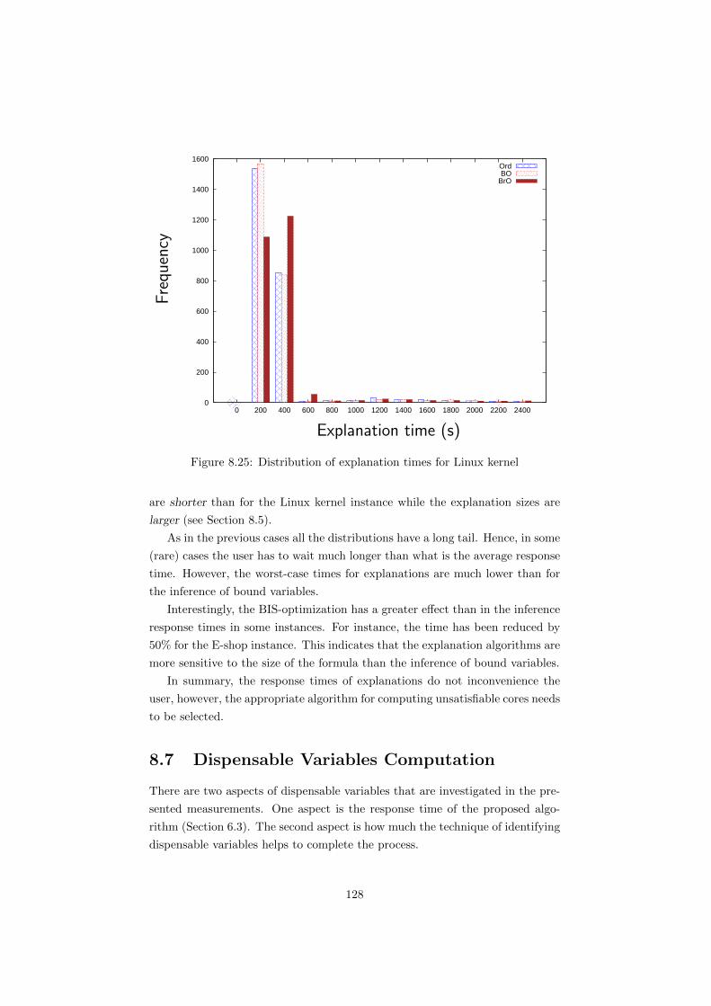
Frequ
ency
0
200
400
600
800
1000
1200
1400
1600
0 200 400 600 800 1000 1200 1400 1600 1800 2000 2200 2400
OrdBO
BrO
Explanation time (s)
Figure 8.25: Distribution of explanation times for Linux kernel
are shorter than for the Linux kernel instance while the explanation sizes are
larger (see Section 8.5).
As in the previous cases all the distributions have a long tail. Hence, in some
(rare) cases the user has to wait much longer than what is the average response
time. However, the worst-case times for explanations are much lower than for
the inference of bound variables.
Interestingly, the BIS-optimization has a greater effect than in the inference
response times in some instances. For instance, the time has been reduced by
50% for the E-shop instance. This indicates that the explanation algorithms are
more sensitive to the size of the formula than the inference of bound variables.
In summary, the response times of explanations do not inconvenience the
user, however, the appropriate algorithm for computing unsatisfiable cores needs
to be selected.
8.7 Dispensable Variables Computation
There are two aspects of dispensable variables that are investigated in the pre-
sented measurements. One aspect is the response time of the proposed algo-
rithm (Section 6.3). The second aspect is how much the technique of identifying
dispensable variables helps to complete the process.
128

As in the case of measurements of the response times for inference of bound
variables, the Linux kernel instance was measured separately. First, let us look
at the small instances (E-shop, Violet, Berkeley, T-shirt, rocket, and 3blocks).
The time aspect is measured as for the response time all the inference of
bound variables with the difference that only one version of optimizations is
investigated; in particular the version BCO. The helpfulness of the technique
is measured by recording the percentages of dispensable variables out of the
variables that are not bound. In particular, if 100% of the unbound variables
are dispensable, then invoking the shopping principle function binds all the
unbound variables and consequently completes the configuration process.
Unlike in the case of computation of bound literals, the computation of
dispensable variables sometimes does not succeed, it times out. For the purpose
of the measurement, the timeout of 1 second was used. The motivation for
choosing this particular timeout was twofold. Firstly, long waiting time for a
technique that is supposed to speed up the configuration process defeats the
purpose of the technique. Secondly, according to previous experience if the
computation does not terminate quickly, then it takes unbearably long.
Interestingly enough, the only instance where some of the cases timed out
was the E-shop feature model. A time out occurred in 1577 cases, which forms
approximately 22% out of the 7215 cases investigated (Table 8.2).
The results of the measurements are again captured as distributions. For
each instance there is an distribution of the percentages of dispensable variables.
And, for each instance there is a distribution of computation times. However,
here we present only the time distributions for the SAT instances, E-shop, and
Berkeley since for all the other instances all cases were computed within 5 ms.
Computing Dispensable Variables for Linux Kernel Since the Linux
kernel instance is significantly larger than the other evaluated instances, the
timeout was increased to 3 seconds. However, despite of this increase the tech-
nique times out in most of the observed cases. Figure 8.28 depicts the distri-
bution of response times and percentages of dispensable variables for the Linux
kernel instance.
8.7.1 Discussion
The percentages of dispensable variables are somewhat surprising (Figure 8.26).
All of the feature model instances have many dispensable variables in many
cases. In the case of Berkeley the dispensable variables form 100% of the un-
bound variables most of the time and in the case of Violet it is even all the
time. All features in this model are optional so such behavior is expected (see
129

Frequ
ency
(a) Distribution for E-shop
0
500
1000
1500
2000
2500
0 10 20 30 40 50 60 70 80 90 100 N/A
dispensables for Eshop-fm.xml (b) Distribution for Violet
0
500
1000
1500
2000
2500
3000
0 10 20 30 40 50 60 70 80 90 100 N/A
dispensables for violet_model.m
Percentage of dispensable variables
Frequ
ency
(c) Distribution for Berkeley
0
100
200
300
400
500
600
700
800
900
0 10 20 30 40 50 60 70 80 90 100 N/A
dispensables for berkeley.m (d) Distribution for T-shirt
0
20
40
60
80
100
120
140
0 10 20 30 40 50 60 70 80 90 100 N/A
dispensables for TShirt.m
Percentage of dispensable variables
Frequ
ency
(e) Distribution for rocket
0
50
100
150
200
250
300
350
0 10 20 30 40 50 60 70 80 90 100 N/A
dispensables for sat_rocket_ext.b.cnf (f) Distribution for 3blocks
0
50
100
150
200
250
300
0 10 20 30 40 50 60 70 80 90 100 N/A
dispensables for 3blocks.cnf
Percentage of dispensable variables
Figure 8.26: Distributions of percentages of dispensable variables
130
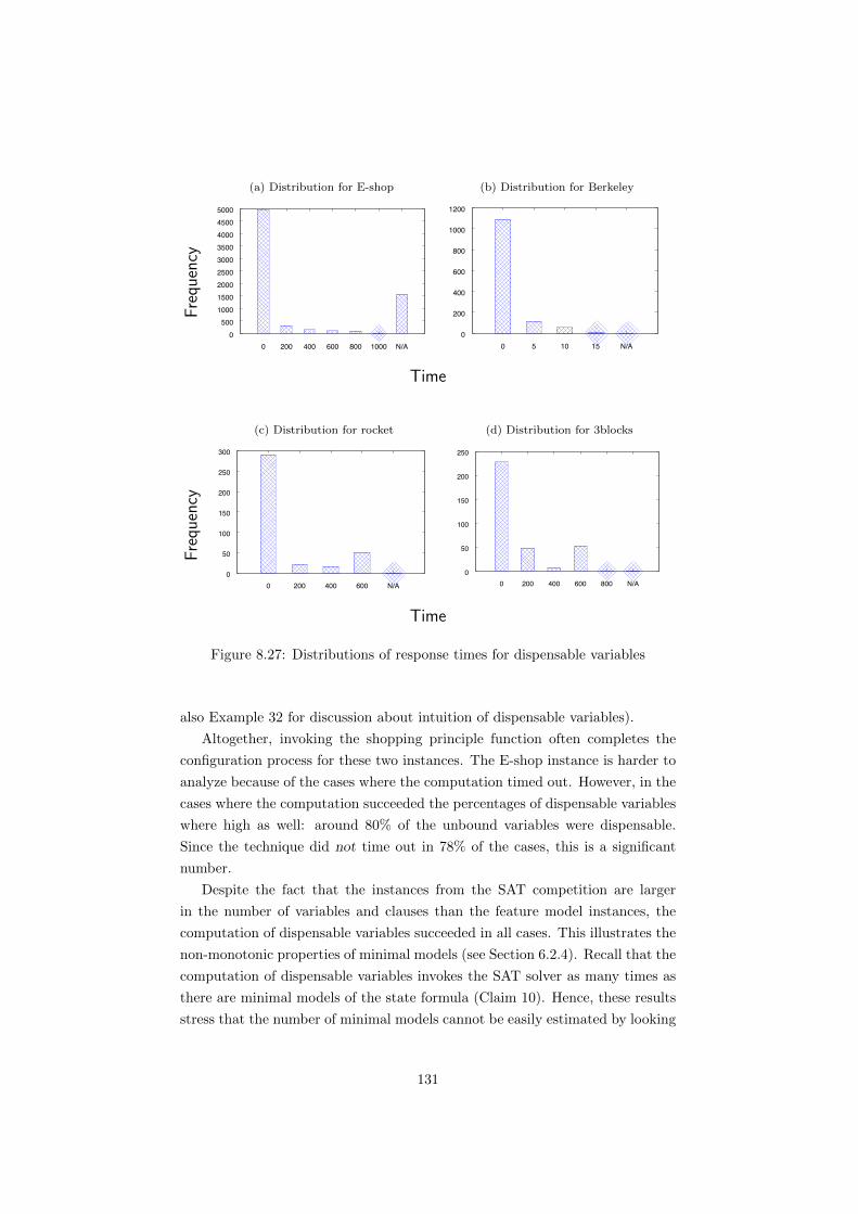
Frequ
ency
(a) Distribution for E-shop
0 500
1000 1500 2000 2500 3000 3500 4000 4500 5000
0 200 400 600 800 1000 N/A
time for Eshop-fm.xml (b) Distribution for Berkeley
0
200
400
600
800
1000
1200
0 5 10 15 N/A
time for berkeley.m
Time
Frequ
ency
(c) Distribution for rocket
0
50
100
150
200
250
300
0 200 400 600 N/A
time for sat_rocket_ext.b.cnf (d) Distribution for 3blocks
0
50
100
150
200
250
0 200 400 600 800 N/A
time for 3blocks.cnf
Time
Figure 8.27: Distributions of response times for dispensable variables
also Example 32 for discussion about intuition of dispensable variables).
Altogether, invoking the shopping principle function often completes the
configuration process for these two instances. The E-shop instance is harder to
analyze because of the cases where the computation timed out. However, in the
cases where the computation succeeded the percentages of dispensable variables
where high as well: around 80% of the unbound variables were dispensable.
Since the technique did not time out in 78% of the cases, this is a significant
number.
Despite the fact that the instances from the SAT competition are larger
in the number of variables and clauses than the feature model instances, the
computation of dispensable variables succeeded in all cases. This illustrates the
non-monotonic properties of minimal models (see Section 6.2.4). Recall that the
computation of dispensable variables invokes the SAT solver as many times as
there are minimal models of the state formula (Claim 10). Hence, these results
stress that the number of minimal models cannot be easily estimated by looking
131
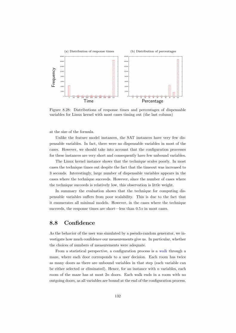
Frequ
ency
(a) Distribution of response times
0
20000
40000
60000
80000
100000
120000
140000
160000
0 400 800 1200 1600 2000 2400 2800 3200 3600 N/A
Time
(b) Distribution of percentages
0
20000
40000
60000
80000
100000
120000
140000
160000
0 10 20 30 40 50 60 70 80 90 100 N/A
Percentage
Figure 8.28: Distributions of response times and percentages of dispensablevariables for Linux kernel with most cases timing out (the last column)
at the size of the formula.
Unlike the feature model instances, the SAT instances have very few dis-
pensable variables. In fact, there were no dispensable variables in most of the
cases. However, we should take into account that the configuration processes
for these instances are very short and consequently have few unbound variables.
The Linux kernel instance shows that the technique scales poorly. In most
cases the technique times out despite the fact that the timeout was increased to
3 seconds. Interestingly, large number of dispensable variables appears in the
cases where the technique succeeds. However, since the number of cases where
the technique succeeds is relatively low, this observation is little weight.
In summary the evaluation shows that the technique for computing dis-
pensable variables suffers from poor scalability. This is due to the fact that
it enumerates all minimal models. However, in the cases where the technique
succeeds, the response times are short—less than 0.5 s in most cases.
8.8 Confidence
As the behavior of the user was simulated by a pseudo-random generator, we in-
vestigate how much confidence our measurements give us. In particular, whether
the choices of numbers of measurements were adequate.
From a statistical perspective, a configuration process is a walk through a
maze, where each door corresponds to a user decision. Each room has twice
as many doors as there are unbound variables in that step (each variable can
be either selected or eliminated). Hence, for an instance with n variables, each
room of the maze has at most 2n doors. Each walk ends in a room with no
outgoing doors, as all variables are bound at the end of the configuration process.
132

Name noop BIS CatE-shop 53.76± 1.08 42.59± 0.78 53.96± 1.07Violet 17.73± 3 16.74± 2.44 17.64± 2.73Berkeley N/A 16.46± 4.87 N/AT-shirt 9.01± 0.65 7.97± 0.62 9.7± 0.823blocks 706.86± 63.39 663.88± 59.25 599.1± 50.97rocket 185.42± 21.33 182.9± 21.17 176.05± 19.84
Name Ord BCOE-shop 9.45± 0.07 7.98± 0.07Violet N/A N/ABerkeley 11.53± 5 8.41± 3.17T-shirt 6.49± 0.55 N/A3blocks 3649.35± 345.5 2847.86± 268.77rocket 298.62± 39.51 285.08± 35.37
Name O BO BrOLinux kernel 1266.87± 56.66 1311.18± 62.23 1308.38± 68.86
Table 8.4: 99% confidence intervals for average response time in a walk in mil-liseconds. “N/A” marks cases that do not pass the Anderson-Darling normalitytest.
In our measurements we simulated 50 random walks.
To determine whether the chosen number is adequate, we investigate how
the average response time differs from one walk to another. Intuitively, if the
observed average times of evaluated walks were dramatically different, our confi-
dence in the measurements would be low since a new walk would be more likely
to be different from those that we evaluated. On the other hand, if the average
times of the evaluated walks are close to each other, a new walk is likely to have
similar characteristics to the ones that were evaluated.
To back this intuition with theory, we assume that the average response time
of a walk is normally distributed over all possible walks and compute confidence
intervals. In order to verify that that the averages are normally distributed
Anderson-Darling test of normality [2] at 5% level2 was used.
Since the test is recommended to be performed on a sample of less than 25
elements, 20 averages out of the 50 observed were sampled at random. A major-
ity of the samples passed the normality test with a few exceptions (Table 8.4).
However, the distributions breaking normality are all of short response times
(less than 100 ms), where more erratic behavior is to be expected and precision
is less of importance (for the time distributions and averages see Section 8.3).
2As is common in statistics, Anderson-Darling test tries to reject the hypothesis that thedistribution is normal. The test produces a numerical value which indicates a deviation fromthe normal distribution. If this value exceeds a certain constant cp, normality is rejected withthe probability 1− p.
133
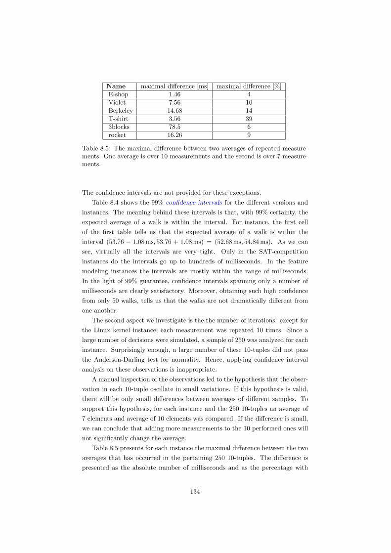
Name maximal difference [ms] maximal difference [%]E-shop 1.46 4Violet 7.56 10Berkeley 14.68 14T-shirt 3.56 393blocks 78.5 6rocket 16.26 9
Table 8.5: The maximal difference between two averages of repeated measure-ments. One average is over 10 measurements and the second is over 7 measure-ments.
The confidence intervals are not provided for these exceptions.
Table 8.4 shows the 99% confidence intervals for the different versions and
instances. The meaning behind these intervals is that, with 99% certainty, the
expected average of a walk is within the interval. For instance, the first cell
of the first table tells us that the expected average of a walk is within the
interval (53.76 − 1.08 ms, 53.76 + 1.08 ms) = (52.68 ms, 54.84 ms). As we can
see, virtually all the intervals are very tight. Only in the SAT-competition
instances do the intervals go up to hundreds of milliseconds. In the feature
modeling instances the intervals are mostly within the range of milliseconds.
In the light of 99% guarantee, confidence intervals spanning only a number of
milliseconds are clearly satisfactory. Moreover, obtaining such high confidence
from only 50 walks, tells us that the walks are not dramatically different from
one another.
The second aspect we investigate is the the number of iterations: except for
the Linux kernel instance, each measurement was repeated 10 times. Since a
large number of decisions were simulated, a sample of 250 was analyzed for each
instance. Surprisingly enough, a large number of these 10-tuples did not pass
the Anderson-Darling test for normality. Hence, applying confidence interval
analysis on these observations is inappropriate.
A manual inspection of the observations led to the hypothesis that the obser-
vation in each 10-tuple oscillate in small variations. If this hypothesis is valid,
there will be only small differences between averages of different samples. To
support this hypothesis, for each instance and the 250 10-tuples an average of
7 elements and average of 10 elements was compared. If the difference is small,
we can conclude that adding more measurements to the 10 performed ones will
not significantly change the average.
Table 8.5 presents for each instance the maximal difference between the two
averages that has occurred in the pertaining 250 10-tuples. The difference is
presented as the absolute number of milliseconds and as the percentage with
134

respect to the average over 10 measurements.
We can see that in most of the instances the difference is less than 10%
and less than 20 ms. The only instance with an excessive difference is the toy
example T-shirt. That is not surprising because the response times for this
instance are in units of milliseconds.
Hence, we can conclude that repeating each measurement 10 times is suf-
ficient because adding more measurements does not significantly influence the
value of the average.
8.9 Presenting Explanations
By automatically selecting or eliminating features the configurator provides
comfort to the user and makes the configuration process less error-prone. How-
ever, there are cases where a user does not find a particular automatic choice
satisfactory [159, 163, 199]. In such situations, the user may want to change
some of the previous decisions in order to reverse the automatic choice. If the
user is also the designer of the feature model, he or she may decide to modify
the model. In either case, the user must understand why the configurator made
the automatic choice in question.
This section compares different types of explanations and argues that expla-
nations based on resolution trees (Section 4.5) provide greater level of informa-
tion to the user.
Figure 8.29 presents a simplified feature model of a car where the user may
pick between manual and automatic gearshift and between electric and gas
engine. The feature model tells us that an engine must be either electric or
gas and analogously the gearshift must be either manual or automatic. An
additional cross-tree constraint tells us that an electric engine excludes manual
gearshift (mutual exclusion).
The figure depicts a situation where the user selected the manual gearshift.
The selection of this feature together with the semantics of the feature model
determines the values for all the other features. Let us focus on the following
question asked by the user:
Why is Gas automatically selected?
Humans typically reason from the consequence in question towards the root
causes. In the case of feature models, this means starting from the feature in
question and by applying the semantics of feature models going toward user
decisions. Using this reasoning, the explanation for automatic selection of Gas
takes the following form.
135
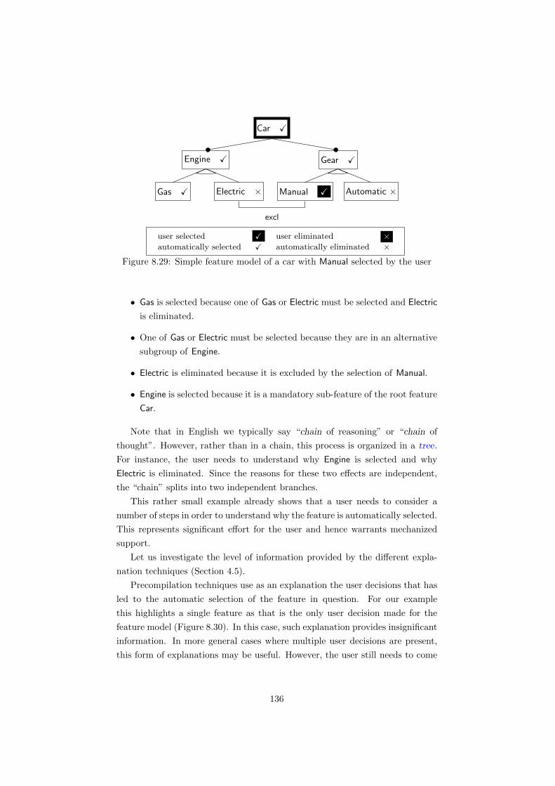
Car X
Engine X
Gas X Electric ×
Gear X
Manual X Automatic ×
excl
user selected X user eliminated ×automatically selected X automatically eliminated ×
Figure 8.29: Simple feature model of a car with Manual selected by the user
• Gas is selected because one of Gas or Electric must be selected and Electric
is eliminated.
• One of Gas or Electric must be selected because they are in an alternative
subgroup of Engine.
• Electric is eliminated because it is excluded by the selection of Manual.
• Engine is selected because it is a mandatory sub-feature of the root feature
Car.
Note that in English we typically say “chain of reasoning” or “chain of
thought”. However, rather than in a chain, this process is organized in a tree.
For instance, the user needs to understand why Engine is selected and why
Electric is eliminated. Since the reasons for these two effects are independent,
the “chain” splits into two independent branches.
This rather small example already shows that a user needs to consider a
number of steps in order to understand why the feature is automatically selected.
This represents significant effort for the user and hence warrants mechanized
support.
Let us investigate the level of information provided by the different expla-
nation techniques (Section 4.5).
Precompilation techniques use as an explanation the user decisions that has
led to the automatic selection of the feature in question. For our example
this highlights a single feature as that is the only user decision made for the
feature model (Figure 8.30). In this case, such explanation provides insignificant
information. In more general cases where multiple user decisions are present,
this form of explanations may be useful. However, the user still needs to come
136

Car X
Engine X
Gas X Electric ×
Gear X
Manual X Automatic ×
excl
Manual X
user selected X user eliminated ×automatically selected X automatically eliminated ×
Figure 8.30: Simple feature model of a car with Manual selected by the userwhere elements responsible for the automatic selection of Gas highlighted. Theexplanation is in the form of pertaining user decisions. In this case it is thesingle Manual that is highlighted as an explanation.
Gas
¬Electric Electric ∨ Gas
Manual ¬Manual ∨ ¬Electric Engine⇒(Electric ∨ Gas)Engine
Car Car⇒Engine
Figure 8.31: Resolution-based explanation for Gas being selected automaticallyin the form of the semantics of the feature model
up with the pertaining relations between the modeling primitives of the feature
model in order to fully understand why the automatic choice has been made.
8.9.1 Resolution Trees
Section 4.5 proposes the use of resolution trees as forms of explanations. First,
let us look at the resolution tree for our question: Why is Gas selected (Fig-
ure 8.31)? The resolution tree is close to the “tree” of thought outlined above.
The clause Gas is obtained by resolving ¬Electric and Electric∨Gas. The clause
¬Electric corresponds to elimination of Electric and Electric∨Gas corresponds to
the fact that at least one of Electric, Gas must be selected. Following the reso-
lution steps towards the leaves in an analogous fashion, all nodes are gradually
explained.
The resolution tree itself is already a helpful information for the user but
137

sel(Gas)
elim(Electric) constraint(Electric ∨ Gas)
sel(Manual) excl(Manual,Electric) alt(Engine, {Electric,Gas})sel(Engine)
root(Car) mandatory(Car,Engine)
Figure 8.32: Resolution-based explanation for Gas being selected automaticallyin the form of modeling primitives
the user interface has a number of options how to present it in that more user-
friendly fashion.
To bring the user closer to the original feature model, the resolution tree,
which is in the form of the semantics of the model (Figure 8.31), can be trans-
lated into a tree of corresponding feature modeling primitives (Figure 8.32).
Such tree is obtained by replacing each clause with the modeling primitive that
generated the clause (see Chapter 7 for the realization of the mapping). The
tree conveys the same information as the original resolution tree but does not
require the user to understand logic notation.
8.9.2 Presenting Resolution Trees
The disadvantage of resolution trees presented so far (Figure 8.31 and Fig-
ure 8.32) is that they are detached from the original feature model. Highlight-
ing in the feature model those primitives that appear in the resolution tree
addresses this disadvantage (Figure 8.33). In order to understand why Gas is
automatically selected, a user follows the primitives marked red and recalls their
respective semantics. The disadvantage of this representation is that the order
of consequences is lost.
Projecting the resolution tree on the feature model addresses this disadvan-
tage (Figure 8.34). This representation combines all the information in one
diagram. Note that an additional node Gas ∨ Electric was added to represent
an intermediate stage of the reasoning3. Such explanation is straightforward to
interpret. Each non-leaf node that is part of the explanation is a consequence
of two reasons. These reasons are those nodes that point to the consequence
via red arrows. For instance, one can immediately see that Electric is selected
because Manual is selected and there is an exclusion edge between Electric and
Manual.
3Such nodes can be removed for less advanced users.
138
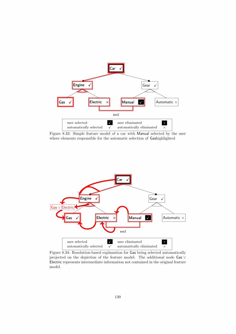
Car X
Engine X
Gas X Electric ×
Gear X
Manual X Automatic ×
excl
Engine X
Electric × Manual X
Car X
Gas X
user selected X user eliminated ×automatically selected X automatically eliminated ×
Figure 8.33: Simple feature model of a car with Manual selected by the userwhere elements responsible for the automatic selection of Gashighlighted
Car X
Engine X
Gas X Electric ×
Gear X
Manual X Automatic ×
excl
Gas ∨ Electric
Engine X
Electric × Manual X
Car X
Gas X
user selected X user eliminated ×automatically selected X automatically eliminated ×
Figure 8.34: Resolution-based explanation for Gas being selected automaticallyprojected on the depiction of the feature model. The additional node Gas ∨Electric represents intermediate information not contained in the original featuremodel.
139

8.9.3 Summary of Explanation Presentation
This section presents the advantages of using resolution trees to provide expla-
nations to the user over just highlighting pertaining user decisions, a technique
used in precompilation methods.
Highlighting the pertaining user decisions that are responsible may represent
a small part of the information that is needed to understand why a certain
feature is automatically selected or eliminated (Figure 8.30).
Presenting explanations as resolution trees enables reasoning akin to the
reasoning that humans use when looking for a root-cause. A user starts from
the feature to be explained and gradually proceeds toward the pertaining user-
decisions.
The user interface has a number of options how to present resolution trees
to the user. The actual resolution tree at the semantic level provides the most
detailed information but requires the user to be familiar with logic (Figure 8.31).
Transforming such resolution tree into a tree of the pertaining modeling prim-
itives conveys the same information but requires only the knowledge of the
modeling primitives (Figure 8.32).
The explanation can be shown on the feature model diagram by highlighting
modeling primitives that appear in the resolution tree (Figure 8.33). Projecting
the resolution tree on the feature model diagram additionally shows reasons
and consequences in the explanation (Figure 8.34). We argue that this last
representation is the most informative one because it shows all the information
in a single diagram.
8.10 Conclusions and Summary
This section discusses the observed behavior from the perspective of the follow-
ing standards coming from the research on acceptable response times [98]:
• 0.1 seconds is classified as instantaneous,
• 1.0 seconds as uninterrupted user action that is noticed by the user but
does not hinder the work, and
• 10 seconds is a limit for keeping user’s attention.
Bound Variables Response Times
For instances with hundreds of variables, we have seen that when computing
bound variables, the configurator responds in 0.1 seconds in many cases and
140
takes over 1 second only in a few cases for hard instances. However, long times—
over 10 seconds—may appear if a wrong heuristic is applied. In particular, the
Ord heuristic does not perform well for the instances from the SAT competition,
which are far more constrained than the variability models.
The evaluation of computation of bound variables for the Linux kernel shows
that the presented approach is applicable in instances with thousands of vari-
ables. The response times for this instance are predominantly around 1 second.
Longer response times appear—up to 10 seconds in several cases. However, such
times are extremely rare—response time exceeded 5 seconds in less than 0.02%
of the inspected cases.
Explanations
The evaluation of explanations for variability models is also satisfactory. The
response times are less than 0.5 second for most of the cases with some rare
exceptions of 2 seconds, which occurred in the Linux kernel instance. The ex-
planation sizes are relatively small. In the largest variability model instance
(Linux kernel) the average explanation size is 16, with some rare exceptions
of the size 100 clauses. However, the evaluation shows that the QuickXplain
algorithm implemented in the solver SAT4J does not scale well and the above
results for the Linux kernel instance were obtained with the tool MUSER (see
Section 7.1).
The evaluation of explanations for the instances from SAT competition show
that the sizes are unwieldy for such types of instances, i.e., instances that are
tightly constrained (the number of clauses is much higher compared to the
number of variables). The sizes of explanations for these instances exceed 232,
which is clearly incomprehensible for a human. In general, such large expla-
nations are most likely inevitable due to the result by Cook and Reckhow ac-
cording to which proofs are super-polynomial in size of the original formula
unless co-NP 6=NP [42]. Nevertheless, the variability models do not exhibit such
excessive explanation sizes.
Section 8.9 demonstrates the usefulness of resolution trees in explanations
already on small examples. The evaluation of the explanation sizes shows that in
real-world instances we can expect explanations counting up to 30 elements and
average around 15 elements. Together these observations show that resolution-
based explanations help the user in many cases.
BIS-optimization
The BIS-optimization shows promising improvements of response times in sev-
eral instances. Unfortunately, the response times for these instances are already
141
short without the optimization. In the large instances (Linux kernel) where
improvement of the response times would be useful, the optimization does not
help.
However, the optimization is interesting from the perspective of explanation
sizes. In some cases reconstructing the explanation from an explanation on the
optimized formula yields a smaller explanation than when the optimization is
not used. This indicates that in some cases the explanation algorithms work
significantly better on smaller formulas.
Dispensable Variables
The analysis of the dispensable variables technique proved the technique to
be fast for instances with hundreds of variables—the response time was below
200 ms in most cases. However, there are some cases where the proposed com-
putation approach fails to deliver results. The technique helps the user to bind
many variables in many cases. In fact, there were many cases where all of the
unbound variables were dispensable, i.e., cases where the shopping principle
function completes the configuration process.
The Linux kernel instance shows that the technique for computing dispens-
able variables does not scale well as it times out in most of the cases. Hence, a
different technique needs to be developed for variability models with thousands
of variables.
Confidence
The analysis of the response times using the methods of confidence intervals
shows that the evaluated sequences differ little from one another. This is impor-
tant from practical perspective because it means that it is possible to accurately
estimate the response times from a small number of observations.
All of the observed distributions have the common property of long tails,
i.e., extreme values occur very rarely. This is a price for the lazy approach
(computation is performed only when needed). However, these tails encompass
small number of cases.
142

Chapter 9
Thesis Evaluation
The statement to be investigated by this dissertation is the following:
SAT solvers are better for implementing a Boolean interactive con-
figurator than precompiled approaches.
In this chapter we argue that the thesis statement is validated by the pre-
sented material. Since we are in the domain of propositional constraints, the
precompiled approaches are represented by BDDs and we show that the advan-
tages of SAT solvers over BDDs are the following:
• SAT solvers scale better,
• SAT solvers are better for providing explanations,
• the response times of the configurator do not make a significant difference,
and
• there is more potential for further research in SAT-based configuration.
These arguments are detailed, in turn, in the following sections.
9.1 Scalability
Examples in Literature
BDDs enabled significant progress in model checking in the early 90s [35, 144].
However, the issue of scalability of BDDs motivated research in the applica-
tion of SAT solvers in model checking. For instance, Abdulla et al. recognize
that BDDs are typically unusable for systems with more than hundreds of vari-
ables [1]. Biere et al. provide an empirical case study where the SAT-based
checker consistently outperforms the BDD-based one [23].
143

Similar trends are appearing in analyses of feature models. Mendonca et al.
study heuristics for compiling feature models into BDDs. The need for such
heuristics is motivated by the poor scalability of BDDs [148]. However, in a
later publication, Mendonca et al. show that SAT solving in feature models is
easy1 [147]. Hence, the motivation for studying heuristics for construction of
BDDs is diminished, since a SAT solver can be used instead. It should be noted,
however, that for some types of analyses, BDDs give better results; an example
of one such analysis is the counting of all possible solutions of an instance [20].
Theoretical Evidence
As mentioned in the background section, the size of a BDD depends on the
ordering of variables in the tree’s branches (Section 2.2.2). It is well-known
that deciding whether a variable ordering is optimal or not is NP-complete [26].
Also, exponential lower bounds are known for the size of BDDs [33]. This further
discourages the use of BDDs, since large amount of data needs to be included
with the instance to be configured.
Despite the empirical evidence that SAT solvers are applicable in more cases
in practice than BDDs, theoretical understanding of such is limited. Neverthe-
less, there are some theoretical results that indicate that constructing a BDD is,
in general, significantly more difficult than deciding satisfiability. The argument
stems from the fact that having a BDD enables us to calculate in linear time
the number of models of the pertaining formula, and, calculating the number of
models is a #P-complete problem2 [194, 162]. The difficulty of solving a #P-
complete problem is illustrated by Toda’s theorem, whose direct consequence
is that a Turing machine with a #P oracle can solve any problem in polyno-
mial hierarchy in polynomial time [191]. Hence, a BDD oracle enables us to
answer any problem in polynomial hierarchy in polynomial time. In contrast
to that, problems already in the second level of polynomial hierarchy require
super-polynomial (in practice exponential) queries to a SAT oracle. While this
is not a formal proof of the fact that constructing a BDD is harder than SAT,
it lends credence to such hypothesis, as there is a significant difference in the
power of the corresponding oracles.
1The notion of easy and hard SAT instances is based on a well-known phenomena thatthe hardness of an instance depends on the ratio of the number of variables to the number ofclauses [155].
2#P is a class of problems that are defined as computing the number of accepting pathsof a nondeterministic Turing machine that is running in polynomial time.
144

Evaluated Instances
The conducted experiments show that the SAT-based approach successfully
copes with all the evaluated instances. In contrast to that, construction of a
BDD from the Linux kernel instance did not succeed even after 24 hours of
computation time using a tool provided by Grigore [170]. As mentioned in the
introduction, the fact that the particular tool did not succeed building the BDD
does not mean that it is impossible. It might be that some heuristics specific to
that instance will succeed in precompiling it. However, the SAT-based approach
scales uniformly , as no heuristics specific to the instances were applied. Thus,
the SAT-based approach is more practical as it imposes fewer requirements on
the user.
Another argument for scalability of the SAT-based approach is the growth of
configurator’s response times that is observed in the evaluated instances. In fea-
ture models with hundreds of variables the times were in the range of 0–200 ms,
while they are predominantly in the range of 0.5–2 s for the large example with
over eight thousand variables. This means that the times grew linearly with
the size of the problem, rather than exponentially as the complexity class of
the problem suggests. This further corroborates the above-mentioned findings
of Mendonca et al. that the SAT problem is easy for variability models [147].
9.2 Providing Explanations
We have shown how explanations are produced from resolution-based proofs
(Section 4.5). Compared to existing work, the provided explanations are more
informative since they comprise parts of the configured instance and depen-
dencies between them. The following paragraphs summarize the capabilities of
SAT-based solutions and the issues with BDDs from the perspective of resolu-
tion proofs.
To produce resolution-based proofs for state-of-the-art SAT solvers is natu-
ral [206]. In fact, a number of popular solvers produce such proofs [167, 151, 107].
Some solvers do not produce a resolution tree, but instead produce an unsatis-
fiable core (unsatisfiable subsets of the given clauses) [111, 140, 142]. In order
to enable constructing a tree from such unsatisfiable core, we provide a SAT
solver that constructs a tree once invoked on the core [102].
Existing research shows that it possible to produce proofs of unsatisfiability
from BDDs [186, 112]. However, there are several issues with this technique.
• The resulting proof is not a standard resolution tree, but instead it is an ex-
tended resolution tree (using the operations of extended resolution) [192].
It is not clear how to compute explanations from such proofs.
145
• The extended-resolution-based proof is obtained from a BDD certifying
unsatisfiability. Such a tree comprises a single node labeled with False.
However, the algorithms for interactive configuration based on BDDs do
not explicitly construct such BDD [92, 189, 88, 187, 188]. The complex-
ity requirements for constructing such tree are unclear, especially in the
presence of proof construction.
• The commonly-used BDD libraries do not support such proof generation.
Hence, when using BDDs in interactive configuration, the explanations can
only be given in the form of user decisions responsible for the queried locked
variable. This gives little information to the user as it is necessary to also
consider the configured instance in order to understand the reason for the lock
(see section on explanations for further details Section 4.5).
9.3 Response Times
The research on applying BDDs to interactive configuration is often motivated
by guaranteed response time, i.e., once a BDD is built, the response time is
known, since the algorithms providing feedback in interactive configuration re-
quire time linear to the size of the BDD. We argue that this motivation is of
little importance as the times obtained in our measurements for the SAT-based
approach were predominantly within the range of hundreds of milliseconds for
the models for which BDDs compile. According to research on human inter-
faces, such response times do not pose any inconvenience upon the user [98].
Moreover, even though the SAT-based approach does not provide a theoretical
guarantee for the response time, the empirical evaluation shows that the re-
sponse times for user decision sequences differ very little from one sequence to
another (Section 8.8). Hence, it is possible to estimate the response time for a
particular instance with high accuracy.
The Linux kernel variability model is currently the largest variability model
available in the research community. Even in the case of this large instance,
the response times were predominantly in the range of 0.5–2 s. According to
research on human interfaces, such times are acceptable for the user—Hoover
classifies such times as “uninterrupted user actions, they will notice a delay but
can continue to work” [98]. Finally, we believe that these times can be improved
by reengineering—for instance, by using a more efficient programming language
than Java for the implementation.
146
9.4 Potential for Further Research
While it is difficult to provide hard evidence that there is more potential for
further research in the SAT-based approach than in the BDD-based approach,
we argue that it is indeed the case.
SAT solvers are used as basis for numerous solvers for non-propositional
logic. Such solvers either by translate the given problem into propositional logic
or extend a SAT solver (see Section 10.5 for further details). We conjecture that
the techniques used in such solvers can be used to extend our approach to inter-
active configuration of instances with non-propositional semantics. A prominent
example are pseudo-Boolean constraints, which are constraints that enable us
to express dependencies such as maximal price or weight (see Chapter 11 for
further discussion).
There are numerous opportunities for response time improvements via syn-
tactic optimizations that are commonly used in SAT solving (see Section 10.2
for further references). We have shown how to integrate the BIS-optimization
into a configurator. We have shown that the optimization in some cases leads to
improvements in response times of up to 20%. We conjecture that it is possible
to achieve further improvements by integrating other syntactic optimizations.
9.5 Summary
We argue that the presented work validates the conjecture that using a SAT
solver is better for implementing a Boolean interactive configurator than using
a precompilation approach. In particular, the SAT-based approach scales better
and enables more informative explanations. The presented measurements show
that the motivation for the precompilation approach, i.e., guaranteed response
time, is of little importance due to the following facts:
• The response times observed in the SAT solution are satisfactory.
• Different inputs from the user produce highly similar response times.
Hence, while the SAT-based approach does not provide a theoretical guarantee
for response times, in practice it is possible to estimate the response times with
high accuracy, and, the response times observed on the evaluated instances do
not inconvenience the user.
Consequently, from the perspective of a programmer that is implementing
a configurator, the SAT approach is more practical. To obtain good response
times for instances counting hundreds of variables, it is sufficient to use a simple
algorithm that requires no heuristics and uses the SAT solver as a black-box. To
obtain good response times for instances counting thousands of variables, it is
147

sufficient to slightly modify the underlying SAT solver. In contrast to that, using
precompilation with large instances requires specific heuristics or modifications
of the underlying data structure. Finally, in both types of instances large and
small, SAT solvers enable more informative explanations.
148

Chapter 10
Related Work
The related work is organized according to the order of the chapters in this
dissertation. Section 10.1 overviews the research done in configuration with
the emphasis on interactive configuration. Section 10.2 overviews research in
formula optimizations akin to the BIS-optimization (Chapter 5). Section 10.3
discusses research related to the chapter on the completion of a configuration
process (Chapter 6) and in particular to research on the computation of dis-
pensable variables (Section 6.3). Section 10.4 points to research related to the
chapter on the construction of the configurator (Chapter 7).
10.1 Configuration
There is a close relation between configuration and backtracking. In the case
of backtracking, an algorithm is exploring the state-space in order to find a
solution to the given problem. Backtracking algorithms often employ heuristics
to determine where to look first [173] and propagation techniques to avoid parts
of the state-space that certainly do not contain a solution [122]. In configuration,
it is the user who determines the order of search and the configurator’s task is
to warn the user about decisions leading to parts with no solution.
From this perspective, configurators are similar to Assumption-Based Truth
Maintenance Systems (ATMSs) introduced by de Kleer [52]. An ATMS is a
generic data structure to be used with a backtracking algorithm. An ATMS is
used by the algorithm to store information obtained during the search so it can
be reused later to avoid duplicate calculation and to avoid sub-spaces without
solutions.
Another correspondence between configuration and backtracking is the con-
cept of backtrack-freeness, which originally comes from research on backtracking
by Freuder [75]. A CSP problem is backtrack-free if there exists an ordering
149

of the variables such that any algorithm assigning values in this order while
preserving consistency of what has been assigned so far, always finds a solution.
The notion of backtrack-freeness in the context of configuration (see Section 3.1)
is stronger because a backtrack-free configurator must ensure this property for
any ordering that the user might choose.
The concept of configuration or interactive configuration appears in multiple
domains. Probably the oldest flavor of configuration is product configuration. In
product configuration the task is to assemble a product from a set of components
which can be connected through their ports while some constraints must be
respected. The bulk of research on product configuration deals with cataloging
the components but such issues are not considered in this dissertation. See
an extensive survey on product configuration by Sabin and Weigel for further
reference [175].
Lottaz et al. focus on configuration of non-discrete domains in civil engi-
neering [131]. They have applied Fourier-Motzkin elimination to support a civil
engineer in the design of an apartment. Such design must conform to certain
constraints, e.g., minimal sizes or distances. These constraints are captured as
linear inequalities. Additionally, non-linear constraints are supported through
approximation.
Another research on interactive configuration of non-discrete domains was
done by Hadzic and Andersen [90]. Compared to Lottaz et al., they take into
account optimization constraints and apply the simplex method [169]. The mo-
tivational example they use is the diet problem—a problem of finding a diet plan
for soldiers with minimal cost and which satisfies certain dietary constraints.
Despite of the promising results of the two promising works referenced above,
it seems that configuration of non-discrete domains is rarely needed. This es-
pecially true in configuration of software where domains are typically not only
discrete but also finite (some exceptions to this are mentioned below).
Finiteness and discreteness of make the search space amenable to precom-
pilation. The motivation for precompilation is that if a constraint is compiled
into a specialized data structure, some computationally hard problems become
easier [49]. In particular, Vempaty showed that a CSP can be compiled into a
finite automaton, often referred to as the Vempaty automaton [197].
Building on Vempaty’s research, Amilhastre et al. show how to perform
interactive configuration on a CSP by first compiling it into a Vempaty au-
tomaton [3]. Other authors take similar approach. Fargier and Vilarem use
tree-driven automata instead of general finite automata to reduce the size of the
automaton [65]; Madsen uses uniform acyclic networks [136]. Pargamin studies
precompilation into cluster tree scheme in the presence of objective function
maximization or optimization in order to configure a CSP [164].
150

One of the most popular data structures for precompilation are Binary De-
cision Diagrams (BDDs) [34]. In general, the size of a BDD may be intractable.
Moreover, finding the smallest BDD is NP-hard [26]. However, both theoret-
ical [86] and experimental [193] research shows that on some problems BDDs
perform better than resolution-based provers but also the other way around.
Remark 10.37. BDDs are a special case of Vempaty automata
because Boolean formulas can be seen as CSPs where all the vari-
ables have the domain {True,False}. However, BDDs are more
attractive for practitioners for their support in the form of libraries
(for instance [109, 108]).
Hadzic et al. show that once a propositional constraint is represented as a
BDD, interactive configuration can be done in time polynomial with respect to
the size of the BDD [92, 189, 88]. In order to cope with the sizes of BDDs,
Subbarayan et al. use trees of BDDs [187] and Join Matched CSPs [188].
Hadzic and Andersen also study global constraints, such as total price, in
the context of propositional configuration and BDDs. The problem they tackle
is to perform configuration while respecting an upper limit on the total cost [89].
Andersen et al. extend the approach to deal with multiple cost functions at the
same time [5].
Van der Meer et al. show that BDDs can be used to implement backtrack-
free and complete configurators even for a certain type of unbounded spaces.
The motivational example they use is a support for constructing component
architectures with arbitrary number of components but that must conform to
some overall constraints [196].
Another example of configuration of unbounded spaces is the configuration
of strings. Hansen et al. show that regular string constraints can be configured
using finite automata [93, 94].
Ensuring backtrack-freeness is in general computationally expensive. In re-
sponse to that, some configurators are not backtrack-free, i.e., the user may run
into a conflict with the original constraint (see Chapter 3). Batory uses unit
propagation (see Section 2.1.3) to provide feedback to the user [15].
Freuder uses arc consistency (AC) (see Section 2.1.4) in the context of
CSP [79]. It is worth noting that AC leads to backtrack-free configuration
for certain types of constraints as shown by Freuder [75]. Freuder et al. also
show that backtrack-freeness can be ensured in the context of AC by removing
certain solutions, i.e., sacrificing completeness of the configurator [77].
Both of these techniques, unit propagation and AC, are not backtrack-free
but are computationally cheap and enable providing nice explanations to the
user. These explanations can be trees similarly as done in this dissertation (see
151
Section 4.5). The approach of Batory and the approach of Freuder are rather
similar due to the relation between unit propagation and arc consistency (see
Section 2.1.5).
If a configurator is not backtrack-free, then the user may run into a conflict—
a situation where the user decisions violate the configured problem. If that is
the case, it is desirable for the configurator to provide support for amending
the conflict. This can be done by constraint relaxation (see for instance [163])
or by corrective explanations (see [159, 199]). Constraint relaxation tries to
remove constraints to restore consistency, while corrective explanations try to
change user decisions, as little as possible, to obtain a consistent set of deci-
sions; corrective explanations are related to the MostClose problem defined
by Herbrard et al. [95].
The research discussed so far is concerned with configuration that yields
one configuration from a space known beforehand. However, there is also re-
search on the synthesis of the outcome. For instance, O’Sullivan uses interactive
constraints propagation in conceptual design [161].
Interactive configuration has also been applied in the context of transfor-
mation. Janota et al. show how interactive support can be used to transform
a propositional logic semantics into a feature model (using BDDs) [106]. The
difficulty in this transformation is that one semantics may correspond to mul-
tiple feature models [48]. The presented solution enables the user to gradually
specify the particular feature model he or she wants.
It should be noted that the research on configuration listed above is in-
evitably incomplete. The problem of configuration seems to be fundamental
as it may be found even in areas rather distant from software engineering, for
example in language parsing [64].
10.1.1 Bound Literals
For a configurator to be complete and backtrack-free, it must identify bound
literals, i.e., literals that evaluate to True under all satisfying assignments of
a formula (see propositions 3 and 2). Bound literals are not only important
in interactive configuration. In the research on the complexity of the SAT
problem, bound literals are known under the name backbones [156, 27, 118].
The correspondence between satisfiability and backbones (see Proposition 1)
has been exploited by Fox et al. [85].
Bound literals are also important in non-interactive configuration. Kaiser
and Kuchlin use the terms inadmissible and necessary variables. A variable v
is inadmissible iff the literal ¬v is bound. Conversely, a variable v is necessary
iff the literal v is bound. Kaiser and Kuchlin use an algorithm similar to Test-
152

Vars to detect bound literals [113].
10.1.2 Proof Size Reduction
As mentioned in Section 4.5, it is desirable to provide explanations as small
as possible since it makes them easier to understand. The explanations are
constructed from the proofs of unsatisfiability, and, these proofs are in the form
of a resolution tree.
As a side note, we mention that the sizes of proofs have a theoretical rele-
vance in particular to the relation co-NP 6=NP shown by Cook and Reckhow [42].
However, since this dissertation is predominantly practical, we refer to practical
proof reduction techniques here.
Ben-Sasson and Wigderson define the width of a resolution tree as the num-
ber of literals in the largest clause appearing in the tree and they show the
relation between tree’s width and its size. Further they propose an algorithm,
based on exhaustive resolution, to derive a resolution tree with the smallest
width [19]. This approach, however, is not directly applicable in modern SAT
solvers as the algorithms behind them are derived from the Davis-Putnam-
Longeman-Loveland Procedure [50].
From an engineering perspective, it is elegant to reduce the size of the resolu-
tion tree returned by the solver since the reduction can be easily integrated into
the configurator as an independent module. Surprisingly, there is little work on
such reduction techniques. Greshman et al. propose to reduce the resolution
tree by repeated calls to the SAT solver [80]. Amjad proposes a compression
technique for resolution proofs [4]. The same is addressed by Sinz but with the
assumption that the proof is obtained from a SAT solver [185]. Bar-Ilan et al.
propose a linear algorithm for reduction of a resolution tree [12].
Another concept related to this discussion are the Minimal Unsatisfiable
Cores (MUS), defined as the subsets of clauses of an unsatisfiable CNF formula
that are unsatisfiable but any of its supersets are satisfiable. Clearly, a proof
that an MUS is unsatisfiable, is also a proof of unsatisfiability of the whole
formula. If the MUS is small, then the proof is likely to be small as well.
A popular technique for approximating an MUS was proposed by Zhang and
Malik [205], which calls the solver again on the proof that it has just produced.
As the proof is an unsatisfiable formula, the solver will find it unsatisfiable and
produce a new proof (possibly smaller than the original one). This process is
iterated until a call to the solver does not affect the size of the proof. The
algorithm QuickXplain proposed by Junker is another popular algorithm to
obtain an MUS or an approximation thereof [111]. Both algorithms, Zhang and
Malik’s and QuickXplain, are practically interesting because they can be added
153

on top of a solver, i.e., the solver serves as a black-box.
There is a large body of research on finding MUSs and the interested reader
is referred to an overview of these techniques by Gregoire et al. [84].
10.2 Related Work for Logic Optimizations
Formula preprocessing techniques are well known in the SAT solver community
(e.g., Several authors focus on binary clauses, i.e., implications, in the context
of satisfiability. Aspvall et al. show that the satisfiability of a CNF formula that
contains only binary clauses can be decided in polynomial time [7]. Both del
Val and Brafman show that satisfiability testing can be sped up if BISs, i.e.,
strongly connected components in the implication graph (see Definition 10), are
collapsed [54, 32]. Bacchus incorporates support for binary clauses into Davis
Putnam procedure by generalizing the notion of resolution [10]
Freuder introduces the concept of interchangeable values in the context of
CSP [76]. Values are interchangeable if changing one to the other in a solution
always yields a solution. This concept is dual to BIS: interchangeable values let
us treat a set of values as one value, BISs let us treat a set of variables as one
variable.
Several authors focus on techniques that preprocess a formula before it is
given to a SAT solver with the goal of making the solver more efficient on the
preprocessed formula. Een and Biere design a technique based on resolution and
it is implemented in the tool SatElite [60]. Fourdrinoy et al. design a technique
that eliminates redundant clauses in polynomial time [71]. For an overview of
simplification techniques for SAT see [133, 134].
To the best knowledge of the author, there has been no research concerned
with reconstructing the proofs from the proof obtained from the optimized for-
mula as is done in Section 5.2.
10.3 Completing a Configuration Process
The work on automated completion of a configuration process is quite limited.
Some authors propose to apply a solver in order to complete the configuration
in some way, i.e., the scenario A as in Section 6.1 [21].
Krebs et al. study the problem of how to help the user to finish the configu-
ration process with the means of machine learning [120]. The learning algorithm
tries to identify a certain plan in the decisions of the user made so far. Once
identified, this plan is used to automatically suggest to them steps in the con-
figuration process.
154

Section 6.4.2 shows that a configuration process may be facilitated if there is
some notion of preference on the possible configurations. Preference as such has
been studied by many researchers and a full discussion on this topic is beyond
the scope of this dissertation. For an overview of formalization of preference in
logic see [55], in CSP see [172], and in human interaction see [166].
Amilhastre et al. enable the user to assign preferences to the decisions. These
preferences then affect the form of explanations [3]. Freuder et al. propose a
preference-based configurator in which different constraints may have different
preferences and the configurator recomputes these preferences after a user de-
cision has been made [78]. The preferences are numbers between 0 and 1 and
are combined using the minimum operator. The proposed configurator does not
find an optimum as it considers soft arc consistency (only pairs of variables are
taken into account).
Junker studies the application of preference in the context of non-interactive
configuration of a CSP [110]. The problem he tackles is that the user is interested
in some solutions of the CSP and the approach Junker suggests is that the user
may specify preferences of how these solutions are searched for using a dedicated
language.
10.3.1 Computing Dispensable Variables
As shown in Chapter 6, dispensable variables are closely related to propositional
circumscription. Originally, circumscription was devised by McCarthy as a form
of reasoning in the ’80s [143]. Minker showed the relation between propositional
circumscription and GCWA in ’82 (a relation shown in Section 6.2.4) [152].
From computational perspective, an important complexity result is that
propositional circumscription is ΠP2 -complete [63]. Moreover, even the query
corresponding to determine whether a variable is dispensable is ΠP2 -complete [63,
Lemma 3.1].
Recall that the algorithm MinModels used in Section 6.3 to compute dis-
pensable variables invokes the SAT solver as many times as there are minimal
models (see Claim 10). Lonc and Truszczynski estimate that the number of
minimal models of a CNF formula is exponential [130].
Giunchiglia and Maratea modify DPLL procedure in an analogous way to
obtain an algorithm similar to the one presented in Section 6.3.1 in order to
solve problems with preference [81]. The problem of finding one minimal model
is a specific instance of the problem solved by these authors. Indeed, Giunchiglia
and Maratea refer to the problem of finding one minimal model as Min-One⊆.
Extending this work, Di Rosa et al. focus on enumerating the most preferred
solutions [171]. The approach is analogous to the one used in Section 6.3, i.e.,
155
finding one minimal model and adding a clause that blocks all models than
the one just found. In fact, this approach has been used as early as 1996 by
Castell et al. in similar context [37].
The main difference between the work on minimal model enumeration refer-
enced in the above paragraph (Castell et al. and Di Rosa et al. ) and Section 6.3
is that these authors modify the DPLL (in the form of a SAT solver) to return
multiple solutions while the approach of Section 6.3 is to invoke the procedure
multiple times. The advantage of modifying the procedure is that some infor-
mation is reused for finding further solutions (such as learned clauses). The
advantage of invoking the procedure is that the algorithm can be used with
different instances of the procedure. Namely, the algorithm can be used with
different SAT solvers or with any procedure that finds a single minimal model
of a formula.
Avin and Zohary solve the problem of propositional circumscription by enu-
merating minimal models [8]. This enumeration is done by exploring possible
models of the formula and testing whether they are indeed minimal; an ordering
of the models is exploited in order to avoid testing all possible models.
Kavvadias et al. show a correspondence between the enumeration of all min-
imal models and traversals of a hyper-graph. Further they devise an output-
polynomial algorithm for enumerating all minimal models of a formula in a
conjunctive normal form that contains only binary clauses [115].
Lee and Lin [124] and show that a propositional circumscription can be
translated into disjunctive logic programs with the stable model semantics
(see [127]). Oikarinen and Janhunen evolve this idea and provide an imple-
mentation connected to an existing implementations of disjunctive logic pro-
gramming [100, 160].
For an overview of calculi and approaches to computation for circumscrip-
tion see at chapter of the Handbook of Automated Reasoning dedicated to this
topic [58]. In a broader perspective, both GCWA and circumscription belong
to the domain of non-monotonic reasoning, see an overview of research in this
area compiled by Minker [153] for more details.
10.4 Building a Configurator
The communication within the reasoning backend starts at the user interface
and ends at the SAT solver. Whenever the user requests an explanation, the
information flows in the opposite direction as well. A similar patterns of data
flow appear in round-trip engineering. In round-trip engineering two forms of
the same information are edited and are kept synchronized. Whenever one of
the forms changes, the other form needs to be automatically updated. This is
156
common in model driven engineering where models and source code need to be
synchronized when the system evolves. For an overview, see a survey by Czar-
necki et al. [45]. In some approaches, the transition from models to source code
is done in multiple steps [145, 119] similarly to the way the semantic translation
is carried out in the reasoning backend. Foster et al. use a technique called lenses
to keep different representations of the same information synchronized [70].
In the semantic translation, however, the translation needs to take into ac-
count the semantic characteristic of the translated elements, whereas the round-
tripping approaches are typically syntactic.
In terms of architecture and workings the reasoning backend is similar to the
verification condition generators. Such generators take a program annotated
with specifications and produce a formula that is valid if the program meets the
specifications; this formula is called the verification condition. This formula is
send to a prover, typically a first-order logic or a higher-order logic prover [67,
13, 40, 68, 73].
When the verification condition is proven not to hold, the generator displays
to the user locations in the program where the specification is violated. A
technique commonly used for providing this kind of feedback is based on labeling
parts of the verification condition. The prover provides a counter-example that
contains the relevant labels and the generator tracks of these labels back to the
source code [126].
10.5 SAT Solvers and their Applications
This section provides pointers to other areas of research where SAT solving
plays an important role. Since it is out of scope of this dissertation to provide
a detailed overview of all these areas, only several exemplars were chosen. An
overview of SAT applications can be found in a recent article by Silva [141] and
an overview of SAT techniques is found in a study by Gu et al. [87].
The potential of SAT solvers started to be apparent in the late 90’s, demon-
strated by such solvers as GRASP [138, 139], SATO [204], or Chaff [158]. Since
then the list of solvers and their power has been growing as can be seen from
the history of the SAT competition [176]. A numerous techniques contributed
to the improvements of efficiency in SAT solvers and the interested reader is
referred to the Handbook of satisfiability for further details [182].
One of the significant domains for application of SAT solvers is the verifica-
tion and testing of electrical circuits. Biere et al. used a SAT solver to model
check properties of a microprocessor [23]. Similarly, Bjesse et al. search for
bugs in an Alpha microprocessor [25]. The application of SAT solvers to model
checking was further studied by Abdulla et al. [1]. Silva and Sakallah show the
157

application of SAT solvers in electronic design automation [183]. Sheeran et al.
verify safety properties using induction [181]. More recently, Dolby et al. applied
SAT solvers in the context of software verification [59].
Another important type of application of SAT solvers is as underlying en-
gines in provers for non-propositional logics. Barrett et al. show that certain
first-order formulas can be proven by a SAT solver by incremental transla-
tion [14]. Satisfiability Modulo Theories (SMT) solvers, such as Z3 or fx7, hinge
on a built-in SAT solver [53, 157]. Lin and Zhao show that answer set program-
ming can be realized using a SAT solver [128]. Wang et al. show that description
logic can be decided using a SAT solver [198].
Recently, SAT solvers were used for problems that are not naturally ex-
pressed in logic; such as cryptography [154], context-free grammars [9], or evo-
lutionary biology [28].
158

Chapter 11
Conclusions and Future
Work
The main motivation of this dissertation is to build a case for using satisfiability
(SAT) solvers to implement interactive configurators. Within a configurator, a
SAT solver is utilized in a lazy fashion, i.e., all computation is carried out during
the configuration process. This contrasts with the precompilation techniques
that do most of the computation before the configuration process starts. While
the precompilation techniques have the advantage of guaranteed response time,
we argue that the lazy approach is more practical.
To support our argument, we show that the lazy approach scales uniformly
without the need of heuristics specific to a particular instance and it is possible
to accurately estimate the response time (Chapter 8). Our approach is also
practical from the implementation point of view. The core algorithms needed
for implementing a configurator based on our principles are lightweight. The
reason why that is the case stems from the fact that most of the computation
takes place in the SAT solver. Hence, by using a SAT solver as the underlying
technology, we are taking advantage of the outstanding progress that took place
in the research on satisfiability in the past two decades. This research not only
resulted in significant improvements in the runtimes of solvers but also in a
number of solvers that are freely available and easy to integrate as third-party
components.
Another benefit that comes from the use of SAT solvers is their ability to
provide resolution-based proofs of unsatisfiability. We demonstrate that such
proofs enable us to produce more informative explanations than those that
are produced by precompilation approaches. In particular, the explanations
contain parts of the instance being configured and dependencies between them
159

as opposed to just user decisions (Chapter 4).
While the concept of interactive configuration is well-known, the study of
completion of a configuration process is neglected in the existing literature. The
dissertation addresses this gap by identifying different scenarios of completion of
a process and formally establishes the notion of “making a choice between num-
ber of options”. Further, we show how a SAT solver is used to identify variables
that can be eliminated without making a choice for the user (Chapter 6).
In conclusion, the dissertation validates the thesis that SAT solvers are better
for implementing Boolean interactive configurators than precompilation-based
approaches by demonstrating scalability and overall practicality of the SAT-
based approach.
In the following sections we point out the potential for future research. Sec-
tions 11.1, 11.3, and 11.4 discuss opportunities for further research from the
technical perspective while Section 11.5 makes more general suggestions for the
research in interactive configuration as a whole.
11.1 Types of Constraints
This dissertation is concerned with interactive configuration of instances that
are captured in propositional logic. A natural direction of future work is to ex-
tend this work with support for non-propositional constraints. An exemplar of
non-propositional constraints are pseudo-Boolean constraints. Pseudo-Boolean
constraints are linear inequalities where variables have the values 0 or 1 (corre-
sponding to False and True, respectively). The following example illustrates
the usefulness of such constraints.
Example 40. Let us have three components. Whether a component is selected
or not is represented by a variable ci, for i ∈ 1..3. Any Boolean constraint can be
expressed as a linear equation. For instance, to express that the first component
requires the second component we write c1 < c2. Let us have a constant price
for each component p1, p2, and p3, respectively. The requirement that the total
price must be at most K is expressed by the equation p1c1 + p2c2 + p3c2 ≤ K.
Any set of pseudo-Boolean constraints can be translated into a Boolean
formula. In principle, such translation may blow up in size. However, there are
numerous successful encoding techniques that enable performing this translation
efficiently [11, 184, 62, 137].
These encoding techniques give us the means to support pseudo-Boolean
constraints in interactive configuration while relying on the techniques described
in this dissertation: applying any of the encodings gives us a Boolean formula to
which all the described algorithms apply. This suggests the following research
160

question: What other types of constraints can be configured using a SAT solver?
11.2 Syntactic Optimizations
The BIS-optimization (Chapter 5) did show some promising results but not
of large significance (Chapter 8). This is an encouragement to study other
optimizations techniques that are known the SAT community (see Section 10.2).
While the effect of such optimizations in SAT solving has been evaluated, the
effect in interactive configuration is expected to be different because the cost of
the optimization is amortized over multiple calls to a SAT solver.
Another topic important in the context of syntactic optimizations is the proof
reconstruction. In the BIS-optimization we provided a way how to reconstruct a
proof for a formula from a proof of its optimized counterpart. We have observed
that the size of the reconstructed proof may vary greatly depending on how the
optimization is carried out. This observation leads to the following research
question: How to provide proofs in the presence of syntactic optimizations,
and, what methods can be employed to reduce the size of the reconstructed
proof?
An interesting phenomenon occurred in some of the instances’ explanation
sizes. When the BIS-optimization was used, in some cases the reconstructed
explanation was smaller than when the optimization was not used (Section 8.5).
This indicates that the algorithms used for computing explanations are sensitive
to the size of the input formula and sometimes perform significantly better when
the formula is smaller. This yields the following research question: What effect
do syntactic optimizations have on proof sizes?
11.3 Dispensable Variables
In Chapter 6, dispensable variables are defined as those variables that can be
eliminated without making a choice for the user (Definition 16). The empir-
ical evaluation shows that the technique for computing dispensable variables
shown in Section 6.3 works well on smaller instances, but scales poorly on the
larger ones (Section 8.7). This encourages further investigation of methods for
computing dispensable variables. Due to the relation of dispensable variables
to propositional circumscription (Section 6.2.4), there are a number of options
to consider [58]. Hence, we propose the following research question: How to
efficiently compute the set of dispensable variables?
161
11.4 Implementation
The separation of concerns provided by the architecture of the configurator
proved to be useful during the development. In particular, it enabled experi-
menting with the implementation by adding or replacing one of the translators
forming the chain of translation. However, at this moment it is the program-
mer who assembles the configurator by modifying the source code. One way of
making this more elegant would be to provide a configuration interface for the
configurator and use some model-driven approach to assemble the configurator.
There is a number of technologies enabling such infrastructure. For instance,
the AHEAD Tool Suite [17] or aspect-oriented programming [125].
11.5 Hindsight and Future
In hindsight, the dissertation is more theory-driven than application-driven.
Namely, the empirical evaluation was carried out at the end of the work. The
disadvantage of this approach is demonstrated by the BIS-optimization. The
optimization proved to be useful in several instances, however, in these instances
the response time is already good from the user perspective without the opti-
mization. Consequently, the dissertation demonstrates the usefulness of the
technique only weakly. Rather, the optimization serves as a proof-of-concept
that shows how to integrate a syntactic optimization into a configurator. If
some preliminary empirical evaluation were performed at the beginning of the
work, the choice of the syntactic optimization would be different.
In a similar regard, little attention was paid to what users of configurators
really need in practice. In fact, there appears to be a large gap between the
research on variability modeling and on application thereof in practice, i.e., a
gap between state-of-the-art and state-of-the-practice.
One such issue comes from models of large sizes. If the configured model con-
tains thousands of variables or more, the model becomes hard to comprehend.
We conjecture that it is possible to use automated reasoning to help users in
such cases. For instance, the most important variables could be automatically
identified according to some criteria.
Another important topic is explanations. The dissertation describes how
to build explanations from resolution trees, and clearly, these explanations are
more informative than explanations comprising only user decisions. However,
we do not understand to what extent such explanations help users in practice.
Moreover, there may exist multiple resolution trees that are semantically equiv-
alent. If that is the case, which of these trees are more intuitive for the user
than the others? More generally speaking, the research questions are: How are
162

explanations useful in practice? and How to present mechanical proofs to a
human?
In conclusion, the research on interactive configuration of variability models
needs to get closer to what is needed in practice. The facets most painfully miss-
ing in this context are benchmarks and user-oriented experiments evaluating the
existing techniques.
163
Bibliography
[1] Parosh Aziz Abdulla, Per Bjesse, and Niklas Een. Symbolic reacha-
bility analysis based on SAT-Solvers. In Susanne Graf and Michael I.
Schwartzbach, editors, TACAS, volume 1785 of Lecture Notes in Com-
puter Science, pages 411–425. Springer, 2000.
[2] NIST/SEMATECH e-handbook of statistical method. http://www.itl.
nist.gov/div898/handbook/.
[3] Jerome Amilhastre, Helene Fargier, and Pierre Marquis. Consistency
restoration and explanations in dynamic CSPs application to configura-
tion. Artificial Intelligence, 135(1-2):199–234, 2002.
[4] Hasan Amjad. Compressing propositional refutations. Electronic Notes
in Theoretical Computer Science, 185:3–15, 2007.
[5] Henrik Reif Andersen, Tarik Hadzic, and David Pisinger. Interactive cost
configuration over decision diagrams. Journal of Artificial Intelligence
Research, 2010.
[6] First Workshop on Analyses of Software Product Lines (ASPL ’08), 2008.
Available at http://www.isa.us.es/aspl08.
[7] Bengt Aspvall, Michael F. Plass, and Robert Endre Tarjan. A linear-time
algorithm for testing the truth of certain quantified boolean formulas. Inf.
Process. Lett., 8(3):121–123, 1979.
[8] Chen Avin and Rachel Ben-Eliyahu-Zohary. Algorithms for computing
X-minimal models. In Logic Programming and Nonmonotonic Reasoning
(LPNMR). Springer, 2001.
[9] Roland Axelsson, Keijo Heljanko, and Martin Lange. Analyzing context-
free grammars using an incremental SAT solver. In ICALP ’08: Proceed-
ings of the 35th international colloquium on Automata, Languages and
Programming, Part II, pages 410–422, Berlin, Heidelberg, 2008. Springer-
Verlag.
164
[10] Fahiem Bacchus. Enhancing davis putnam with extended binary clause
reasoning. In AAAI/IAAI, pages 613–619, 2002.
[11] Olivier Bailleux and Yacine Boufkhad. Efficient CNF encoding of Boolean
cardinality constraints. In Francesca Rossi, editor, CP, volume 2833 of
Lecture Notes in Computer Science, pages 108–122. Springer, 2003.
[12] Omer Bar-Ilan, Oded Fuhrmann, Shlomo Hoory, Ohad Shacham, and Ofer
Strichman. Linear-time reductions of resolution proofs. In Hana Chockler
and Alan J. Hu, editors, Haifa Verification Conference, volume 5394 of
Lecture Notes in Computer Science, pages 114–128. Springer, 2008.
[13] Michael Barnett, Bor-Yuh Evan Chang, Robert DeLine, Bart Jacobs, and
K. Rustan M. Leino. Boogie: A modular reusable verifier for object-
oriented programs. In Frank S. de Boer, Marcello M. Bonsangue, Susanne
Graf, and Willem P. de Roever, editors, FMCO, volume 4111 of Lecture
Notes in Computer Science, pages 364–387. Springer, 2005.
[14] Clark W. Barrett, David L. Dill, and Aaron Stump. Checking satisfiability
of first-order formulas by incremental translation to SAT. In Ed Brinksma
and Kim Guldstrand Larsen, editors, CAV, volume 2404 of Lecture Notes
in Computer Science, pages 236–249. Springer, 2002.
[15] Don Batory. Feature models, grammars, and propositional formulas. In
H. Obbink and K. Pohl, editors, Proceedings of the 9th International
Software Product Line Conference (SPLC ’05), volume 3714 of Lecture
Notes in Computer Science. Springer-Verlag, September 2005.
[16] Don Batory and Sean O’Malley. The design and implementation of hier-
archical software systems with reusable components. ACM Transactions
on Software Engineering and Methodology, 1992.
[17] Don Batory, Jacob Neal Sarvela, and Axel Rauschmayer. Scaling step-wise
refinement. IEEE Transactions on Software Engineering, 30(6), 2004.
[18] Don S. Batory, Vivek Singhal, Jeff Thomas, Sankar Dasari, Bart J. Geraci,
and Marty Sirkin. The GenVoca model of software-system generators.
IEEE Software, 11(5):89–94, 1994.
[19] Eli Ben-Sasson and Avi Wigderson. Short proofs are narrow—resolution
made simple. Journal of the ACM, 48(2):149–169, 2001.
[20] David Benavides, Sergio Segura, and Antonio Ruiz-Cortes. Automated
analysis of feature models 20 years later: A literature review. Inf. Syst.,
35(6):615–636, 2010.
165

[21] David Benavides, Pablo Trinidad, and Antonio Ruiz-Cortes. Automated
reasoning on feature models. In Pastor Oscar and Joao Falcao e Cunha,
editors, Proceedings of 17th International Conference on Advanced Infor-
mation Systems Engineering (CAiSE 05), volume 3520 of Lecture Notes
in Computer Science. Springer-Verlag, 2005.
[22] Thorsten Berger, Steven She, Rafael Lotufo, Andrzej Wasowski, and
Krzysztof Czarnecki. Variability modeling in the real: A perspective from
the operating systems domain. In 25th IEEE/ACM International Confer-
ence on Automated Software Engineering (ASE’10), September 2010.
[23] Armin Biere, Edmund M. Clarke, Richard Raimi, and Yunshan Zhu. Ver-
ifiying safety properties of a Power PC microprocessor using symbolic
model checking without BDDs. In Nicolas Halbwachs and Doron Peled,
editors, CAV, volume 1633 of Lecture Notes in Computer Science, pages
60–71. Springer, 1999.
[24] Armin Biere and Carla P. Gomes, editors. Theory and Applications of
Satisfiability Testing - SAT 2006, 9th International Conference, Seattle,
WA, USA, August 12-15, 2006, Proceedings, volume 4121 of Lecture Notes
in Computer Science. Springer, 2006.
[25] Per Bjesse, Tim Leonard, and Abdel Mokkedem. Finding bugs in an alpha
microprocessor using satisfiability solvers. In CAV ’01: Proceedings of
the 13th International Conference on Computer Aided Verification, pages
454–464, London, UK, 2001. Springer-Verlag.
[26] Beate Bollig and Ingo Wegener. Improving the variable ordering of OBDDs
is NP-complete. IEEE Transactions on Computers, 45(9):993–1002, 1996.
[27] Bela Bollobas, Christian Borgs, Jennifer T. Chayes, Jeong Han Kim, and
David Bruce Wilson. The scaling window of the 2-SAT transition. Random
Structures and Algorithms, 18(3):201–256, 2001.
[28] Maria Luisa Bonet and Katherine St. John. Efficiently calculating evo-
lutionary tree measures using SAT. In Oliver Kullmann, editor, SAT,
volume 5584 of Lecture Notes in Computer Science, pages 4–17. Springer,
2009.
[29] Goetz Botterweck, Denny Schneeweiss, and Andreas Pleuss. Interactive
techniques to support the configuration of complex feature models. In
1st International Workshop on Model Driven Product Line Engineering
(MDPLE), 2009.
166
[30] Goetz Botterweck, Steffen Thiel, Daren Nestor, Saad bin Abid, and Ciaran
Cawley. Visual tool support for configuring and understanding Software
Product Lines. In The 12th International Software Product Line Confer-
ence (SPLC), 2008.
[31] Aaron R. Bradley and Zohar Manna. The Calculus of Computation: Deci-
sion Procedures with Applications to Verification. Springer-Verlag, 2008.
[32] Ronen I. Brafman. A simplifier for propositional formulas with many
binary clauses. IEEE Transactions on Systems, Man, and Cybernetics,
Part B, 34(1):52–59, 2004.
[33] Yuri Breitbart, Harry B. Hunt III, and Daniel J. Rosenkrantz. On the
size of binary decision diagrams representing Boolean functions. Theor.
Comput. Sci., 145(1&2):45–69, 1995.
[34] Randal E. Bryant. Graph-based algorithms for Boolean function manip-
ulation. IEEE Transactions on Computers, 35(8), 1986.
[35] Jerry R. Burch, Edmund M. Clarke, Kenneth L. McMillan, David L. Dill,
and L. J. Hwang. Symbolic model checking: 1020 states and beyond. In
LICS, pages 428–439. IEEE Computer Society, 1990.
[36] Marco Cadoli and Maurizio Lenzerini. The complexity of closed world
reasoning and circumscription. In The Eighth National Conference on
Artificial Intelligence (AAAI), 1990.
[37] Thierry Castell, Claudette Cayrol, Michel Cayrol, and Daniel Le Berre.
Using the Davis and Putnam procedure for an efficient computation of
preferred models. In In ECAI ’96, 1996.
[38] Moses Charikar, Chandra Chekuri, To-Yat Cheung, Zuo Dai, Ashish Goel,
Sudipto Guha, and Ming Li. Approximation algorithms for directed
Steiner problems. In Proceedings of the 9th annual ACM-SIAM sym-
posium on Discrete algorithms, pages 192–200. Society for Industrial and
Applied Mathematics Philadelphia, PA, USA, 1998.
[39] Paul Clements and Linda Northrop. Software Product Lines: Practices
and Patterns. Addison–Wesley Publishing Company, 2002.
[40] Ernie Cohen, Markus Dahlweid, Mark A. Hillebrand, Dirk Leinenbach,
Micha l Moskal, Thomas Santen, Wolfram Schulte, and Stephan Tobies.
VCC: A practical system for verifying concurrent C. In Stefan Berghofer,
Tobias Nipkow, Christian Urban, and Makarius Wenzel, editors, TPHOLs,
167
volume 5674 of Lecture Notes in Computer Science, pages 23–42. Springer,
2009.
[41] Stephen A. Cook. The complexity of theorem-proving procedures. In
STOC ’71: Proceedings of the third annual ACM symposium on Theory
of computing, pages 151–158, New York, NY, USA, 1971. ACM.
[42] Stephen A. Cook and Robert A. Reckhow. The relative efficiency of propo-
sitional proof systems. Journal of Symbolic Logic, 44(1):36–50, 1979.
[43] Krzysztof Czarnecki, Thomas Bednasch, Peter Unger, and Ulrich Eise-
necker. Generative programming for embedded software: An industrial
experience report. In Don Batory, Charles Consel, and Walid Taha, edi-
tors, Proceedings of the ACM SIGPLAN/SIGSOFT Conference on Gen-
erative Programming and Component Engineering (GPCE ’02), volume
2487 of Lecture Notes in Computer Science. Springer Berlin/Heidelberg,
October 2002.
[44] Krzysztof Czarnecki and Ulrich W. Eisenecker. Generative Programming –
Methods, Tools, and Applications. Addison–Wesley Publishing Company,
2000.
[45] Krzysztof Czarnecki, J. Nathan Foster, Zhenjiang Hu, Ralf Lammel, Andy
Schurr, and James F. Terwilliger. Bidirectional transformations: A cross-
discipline perspective. In Richard F. Paige, editor, ICMT, volume 5563 of
Lecture Notes in Computer Science, pages 260–283. Springer, 2009.
[46] Krzysztof Czarnecki, Simon Helsen, and Ulrich Eisenecker. Formalizing
cardinality-based feature models and their staged configuration. Techni-
cal Report 04-11, Department of Electrical and Computer Engineering,
University of Waterloo, Canada, April 2004.
[47] Krzysztof Czarnecki, Simon Helsen, and Ulrich Eisenecker. Staged config-
uration using feature models. In R. L. Nord, editor, Proceedings of Third
International Conference on Software Product Lines (SPLC ’04), volume
3154 of Lecture Notes in Computer Science. Springer-Verlag, August 2004.
[48] Krzysztof Czarnecki and Andrzej Wasowski. Feature diagrams and logics:
There and back again. In Kellenberger [116].
[49] Adnan Darwiche and Pierre Marquis. A knowledge compilation map.
Journal of Artificial Intelligence Research, 2002.
[50] Martin Davis, George Logemann, and Donald Loveland. A machine pro-
gram for theorem-proving. Communication of the ACM, 5(7):394–397,
1962.
168

[51] Merijn de Jonge and Joost Visser. Grammars as feature diagrams. Pre-
sented at the Generative Programming Workshop 2002, Austin, Texas,
April 2002.
[52] Johan de Kleer. An Assumption-Based TMS. Artificial Intelligence,
28(2):127–162, 1986.
[53] Leonardo Mendonca de Moura and Nikolaj Bjørner. Z3: An efficient SMT
solver. In C. R. Ramakrishnan and Jakob Rehof, editors, TACAS, volume
4963 of Lecture Notes in Computer Science, pages 337–340. Springer, 2008.
[54] Alvaro del Val. Simplifying binary propositional theories into connected
components twice as fast. Lecture Notes in Computer Science, pages 392–
406, 2001.
[55] James Delgrande, Torsten Schaub, Hans Tompits, and Kewen Wang. A
classification and survey of preference handling approaches in nonmono-
tonic reasoning. Computational Intelligence, 20(2):308–334, 2004.
[56] Frank DeRemer and Hans Kron. Programming-in-the large versus
programming-in-the-small. In Proceedings of the international conference
on Reliable software, page 121. ACM, 1975.
[57] Edsger W. Dijkstra. A Discipline of Programming. Prentice–Hall, Inc.,
1976.
[58] Jurgen Dix, Ulrich Furbach, and Ilkka Niemela. Nonmonotonic reasoning:
Towards efficient calculi and implementations. In Andrei Voronkov and
Alan Robinson, editors, Handbook of Automated Reasoning, chapter 19,
pages 1241–1354. Elsevier Science, 2001.
[59] Julian Dolby, Mandana Vaziri, and Frank Tip. Finding bugs efficiently
with a SAT solver. In ESEC-FSE ’07: Proceedings of the the 6th joint
meeting of the European software engineering conference and the ACM
SIGSOFT symposium on The foundations of software engineering, pages
195–204, New York, NY, USA, 2007. ACM.
[60] Niklas Een and Armin Biere. Effective preprocessing in SAT through vari-
able and clause elimination. In Theory and Applications of Satisfiability
Testing (SAT ’05). Springer, 2005.
[61] Niklas Een and Niklas Sorensen. An extensible SAT-solver. In Theory and
Applications of Satisfiability Testing (SAT ’03). Springer-Verlag, 2003.
[62] Niklas Een and Niklas Sorensson. Translating Pseudo-Boolean constraints
into SAT. JSAT, 2(1-4):1–26, 2006.
169
[63] Thomas Eiter and Georg Gottlob. Propositional circumscription and ex-
tended closed world reasoning are ΠP2 -complete. Theoretical Computer
Science, 1993.
[64] Mathieu Estratat and Laurent Henocque. Parsing languages with a config-
urator. In Ramon Lopez de Mantaras and Lorenza Saitta, editors, ECAI,
pages 591–595. IOS Press, 2004.
[65] Helene Fargier and Marie-Catherine Vilarem. Compiling CSPs into tree-
driven automata for interactive solving. Constraints, 9(4):263–287, 2004.
[66] Feature model repository web page. http://fm.gsdlab.org.
[67] Jean-Christophe Filliatre and Claude Marche. The Why/Krakatoa/
Caduceus platform for deductive program verification. In Werner Damm
and Holger Hermanns, editors, CAV, volume 4590 of Lecture Notes in
Computer Science, pages 173–177. Springer, 2007.
http://why.lri.fr/.
[68] Cormac Flanagan, K. Rustan M. Leino, Mark Lillibridge, Greg Nelson,
James B. Saxe, and Raymie Stata. Extended static checking for Java. In
PLDI, pages 234–245, 2002.
[69] Kenneth D. Forbus and Johan de Kleer. Building Problem Solvers. MIT
Press, Cambridge, MA, USA, 1993.
[70] J. Nathan Foster, Michael B. Greenwald, Jonathan T. Moore, Benjamin C.
Pierce, and Alan Schmitt. Combinators for bi-directional tree transfor-
mations: a linguistic approach to the view update problem. In POPL ’05:
Proceedings of the 32nd ACM SIGPLAN-SIGACT symposium on Prin-
ciples of programming languages, pages 233–246, New York, NY, USA,
2005. ACM.
[71] Olivier Fourdrinoy, Eric Gregoire, Bertrand Mazure, and Lakhdar Sais.
Eliminating redundant clauses in sat instances. In CPAIOR, pages 71–83.
Springer, 2007.
[72] William B. Frakes and Kyo Kang. Software reuse research: Status and
future. IEEE Trans. Software Eng., 31(7):529–536, 2005.
[73] Frama-C homepage.
http://frama-c.cea.fr/.
[74] Eugene C. Freuder. Synthesizing constraint expressions. Communication
of the ACM, 21(11):958–966, 1978.
170

[75] Eugene C. Freuder. A sufficient condition for backtrack-free search. Jour-
nal of the ACM, 29(1):24–32, 1982.
[76] Eugene C. Freuder. Eliminating interchangeable values in constraint sat-
isfaction problems. In AAAI, pages 227–233, 1991.
[77] Eugene C. Freuder, Tom Carchrae, and J. Christopher Beck. Satisfaction
guaranteed. In Proceedings of the IJCAI-2003 Workshop on Configura-
tion, 2003.
[78] Eugene C. Freuder, Chavalit Likitvivatanavong, Manuela Moretti,
Francesca Rossi, and Richard J. Wallace. Computing explanations and
implications in preference-based configurators. In Barry O’Sullivan, edi-
tor, International Workshop on Constraint Solving and Constraint Logic
Programming, pages 76–92. Springer, 2002.
[79] Eugene C. Freuder, Chavalit Likitvivatanavong, and Richard J. Wallace.
Explanation and implication for configuration problems. In Proceedings of
the 17th Int. Joint Conf. on Artificial Intelligence (IJCAI ’01), Workshop
on Configuration, 2001.
[80] Roman Gershman, Maya Koifman, and Ofer Strichman. Deriving small
unsatisfiable cores with dominators. In Thomas Ball and Robert B. Jones,
editors, CAV, volume 4144 of Lecture Notes in Computer Science, pages
109–122. Springer, 2006.
[81] Enrico Giunchiglia and Marco Maratea. Solving optimization problems
with DLL. In Proceeding of the 2006 conference on ECAI ’06. IOS Press,
2006.
[82] gnuplot—a portable command-line driven graphing utility http://www.
gnuplot.info/.
[83] C.P. Gomes, B. Selman, and H. Kautz. Boosting combinatorial search
through randomization. In Proceedings of the National Conference on
Artificial Intelligence, 1998.
[84] Eric Gregoire, Bertrand Mazure, and Cedric Piette. On approaches to
explaining infeasibility of sets of boolean clauses. In The 20th IEEE In-
ternational Conference on Tools with Artificial Intelligence (ICTAI ’08),
November 2008.
[85] Peter Gregory, Maria Fox, and Derek Long. A new empirical study of
weak backdoors. In International Conference on Principles and Practice
of Constraint Programming, pages 618–623, 2008.
171

[86] Jan Frisco Groote and Hans Zantema. Resolution and binary decision di-
agrams cannot simulate each other polynomially. Discrete Applied Math-
ematics, 130(2):157–171, 2003. The Renesse Issue on Satisfiability.
[87] Jun Gu, Paul W. Purdom, John Franco, and Benjamin W. Wah. Algo-
rithms for the satisfiability (SAT) problem: A survey. DIMACS Series in
Discrete Mathematics and Theoretical Computer Science, 35, 1997.
[88] Tarik Hadzic. Constraint Processing Over Decision Diagrams. PhD thesis,
IT University of Copenhagen, 2007.
[89] Tarik Hadzic and Henrik R. Andersen. A BDD-based polytime algorithm
for cost-bounded interactive configuration. In Proceedings of the National
Conference on Artificial Intelligence. Menlo Park, CA; Cambridge, MA;
London; AAAI Press; MIT Press; 1999, 2006.
[90] Tarik Hadzic and Henrik Reif Andersen. Interactive configuration based
on linear programming. Technical report, IT University of Copenhagen,
2005.
[91] Tarik Hadzic and Henrik Reif Andersen. Interactive reconfiguration in
power supply restoration. In van Beek [195], pages 767–771.
[92] Tarik Hadzic, Sathiamoorthy Subbarayan, Rune M. Jensen, Henrik R.
Andersen, Jesper Møller, and Henrik Hulgaard. Fast backtrack-free prod-
uct configuration using a precompiled solution space representation. In
Proceedings of the International Conference on Economic, Technical and
Organizational aspects of Product Configuration Systems, DTU, pages
131–138, 2004.
[93] Esben Rune Hansen and Henrik R. Andersen. Interactive configuration
with regular string constraints. In AAAI ’07: Proceedings of the 22nd
national conference on Artificial intelligence, pages 217–223. AAAI Press,
2007.
[94] Esben Rune Hansen and Peter Tiedemann. Improving the performance of
interactive configuration with regular string constraints. In Proceedings
of the 2008 20th IEEE International Conference on Tools with Artificial
Intelligence-Volume 01, pages 3–10. IEEE Computer Society, 2008.
[95] Emmanuel Hebrard, Brahim Hnich, Barry O’Sullivan, and Toby Walsh.
Finding diverse and similar solutions in constraint programming. In
Manuela M. Veloso and Subbarao Kambhampati, editors, AAAI, pages
372–377. AAAI Press / The MIT Press, 2005.
172

[96] C.A.R. Hoare. An axiomatic basis for computer programming. Commu-
nications of the ACM, 12:576–580, 1969.
[97] Peter Hofner, Ridha Khedri, and Bernhard Moller. Feature algebra.
In Proceedings of the 14th International Symposium on Formal Meth-
ods (FM), volume 4085 of Lecture Notes in Computer Science. Springer-
Verlag, 2006.
[98] Charles Hoover. A methodology for determining response time baselines.
In Int. CMG Conference, pages 85–94. Computer Measurement Group,
2006.
[99] Katsuro Inoue, Reishi Yokomori, Hikaru Fujiwara, Tetsuo Yamamoto,
Makoto Matsushita, and Shinji Kusumoto. Component rank: relative
significance rank for software component search. In ICSE ’03: Proceed-
ings of the 25th International Conference on Software Engineering, pages
14–24, Washington, DC, USA, 2003. IEEE Computer Society.
[100] Tomi Janhunen and Emilia Oikarinen. Capturing parallel circumscription
with disjunctive logic programs. In Jose Julio Alferes and Joao Alexandre
Leite, editors, JELIA, volume 3229 of Lecture Notes in Computer Science,
pages 134–146. Springer, 2004.
[101] Mikolas Janota and Joseph Kiniry. Reasoning about feature models in
higher-order logic. In Kellenberger [116].
[102] Mikolas Janota. PidiSAT. Available at http://kind.ucd.ie/products/
opensource/Config/releases/.
[103] Mikolas Janota. Do SAT solvers make good configurators? In ASPL08
[6]. Available at http://www.isa.us.es/aspl08.
[104] Mikolas Janota and Goetz Botterweck. Formal approach to integrat-
ing feature and architecture models. In Proceeding of Fundamental Ap-
proaches to Software Engineering (FASE), Lecture Notes in Computer
Science. Springer-Verlag, 2008.
[105] Mikolas Janota, Goetz Botterweck, Radu Grigore, and Joao Marques-
Silva. How to complete an interactive configuration process? In Proceed-
ing of 36th International Conference on Current Trends in Theory and
Practice of Computer Science (SOFSEM). Springer-Verlag, 2010.
[106] Mikolas Janota, Victoria Kuzina, and Andrzej Wasowski. Model construc-
tion with external constraints: An interactive journey from semantics to
syntax. In Krzysztof Czarnecki, Ileana Ober, Jean-Michel Bruel, Axel
173

Uhl, and Markus Volter, editors, MoDELS, volume 5301 of Lecture Notes
in Computer Science, pages 431–445. Springer, 2008.
[107] JatSAT http://www-verimag.imag.fr/~cotton/jat/.
[108] JavaBDD. http://javabdd.sourceforge.net/.
[109] Rune M. Jensen. CLab: A C++ library for fast backtrack-free interactive
product configuration. In Principles and Practice of Constraint Program-
ming (CP ’04). Springer, 2004.
[110] Ulrich Junker. Preference programming for configuration. In Workshop
on Configuration, 2001.
[111] Ulrich Junker. QuickXplain: Conflict detection for arbitrary constraint
propagation algorithms. In Workshop on Modelling and Solving problems
with constraints IJCAI ’01, 2001.
[112] Toni Jussila, Carsten Sinz, and Armin Biere. Extended resolution proofs
for symbolic SAT solving with quantification. In Biere and Gomes [24],
pages 54–60.
[113] Andreas Kaiser and Wolfgang Kuchlin. Detecting inadmissible and nec-
essary variables in large propositional formulae. In Proceedings of Inter-
national Joint Conference on Automated Reasoning: IJCAR 2001 (Short
Papers), 2001.
[114] Kyo C. Kang, Sholom G. Cohen, James A. Hess, William E. Novak, and
A. Spencer Peterson. Feature-oriented domain analysis (FODA), feasibil-
ity study. Technical Report CMU/SEI-90-TR-021, SEI, Carnegie Mellon
University, November 1990.
[115] Dimitris J. Kavvadias, Martha Sideri, and Elias C. Stavropoulos. Gener-
ating all maximal models of a Boolean expression. Information Processing
Letters, 74(3-4):157–162, 2000.
[116] Patrick Kellenberger, editor. Software Product Lines. IEEE Computer
Society, 2007.
[117] Gregor Kiczales, Erik Hilsdale, Jim Hugunin, Mik Kersten, Jeffrey Palm,
and William G. Griswold. An overview of AspectJ. In Proceedings of the
15th European Conference on Object-Oriented Programming (ECOOP),
volume 2072 of Lecture Notes in Computer Science, page 110. Springer-
Verlag, 2001.
174

[118] Philip Kilby, John K. Slaney, Sylvie Thiebaux, and Toby Walsh. Back-
bones and backdoors in satisfiability. In AAAI Conference on Artificial
Intelligence, pages 1368–1373, 2005.
[119] Joseph R. Kiniry and Fintan Fairmichael. Ensuring consistency between
designs, documentation, formal specifications, and implementations. In
The 12th International Symposium on Component Based Software Engi-
neering (CBSE ’09), 2009.
[120] Thorsten Krebs, Thomas Wagner, and Wolfgang Runte. Recognizing user
intentions in incremental configuration processes. In Workshop on Con-
figuration, 2003.
[121] Charles W. Krueger. Software reuse. Computing Surveys, 24(2):131–183,
1992.
[122] Vipin Kumar. Algorithms for constraint-satisfaction problems: A survey.
AI Magazine, 13(1):32–44, 1992.
[123] Gary T. Leavens, Albert L. Baker, and Clyde Ruby. Behavioral Specifi-
cations of Business and Systems, chapter JML: A Notation for Detailed
Design, pages 175–188. Kluwer Academic Publishing, 1999.
[124] Joohyung Lee and Fangzhen Lin. Loop formulas for circumscription. In
Deborah L. McGuinness and George Ferguson, editors, AAAI, pages 281–
286, 2004.
[125] Kwanwoo Lee, Goetz Botterweck, and Steffen Thiel. Feature-modeling
and aspect-oriented programming: Integration and automation. In Haeng-
Kon Kim and Roger Y. Lee, editors, SNPD, pages 186–191. IEEE Com-
puter Society, 2009.
[126] K. Rustan M. Leino, Todd Millstein, and James B. Saxe. Generating error
traces from verification-condition counterexamples. Science of Computer
Programming, 2004.
[127] Vladimir Lifschitz. Foundations of logic programming. Principles of
Knowledge Representation, pages 69–127, 1996.
[128] Fangzhen Lin and Yuting Zhao. ASSAT: computing answer sets of a logic
program by SAT solvers. Artif. Intell., 157(1-2):115–137, 2004.
[129] Jia Liu, Don Batory, and Srinivas Nedunuri. Modeling interactions in
feature oriented software designs. In Proceedings of ICFI, 2005.
175

[130] Zbigniew Lonc and Miros law Truszczynski. Computing minimal models,
stable models, and answer sets. In Catuscia Palamidessi, editor, ICLP, vol-
ume 2916 of Lecture Notes in Computer Science, pages 209–223. Springer-
Verlag, 2003.
[131] Claudio Lottaz, Ruth Stalker, and Ian Smith. Constraint solving and
preference activation for interactive design. Artificial Intelligence for En-
gineering Design, Analysis and Manufacturing (AI EDAM), 12(01):13–27,
1998.
[132] Donald W. Loveland. Automated Theorem Proving: A Logical Basis.
North-Holland Publishing Co., 1978.
[133] Ines Lynce and Joao P. Marques Silva. The puzzling role of simplification
in propositional satisfiability. In Proceedings of the EPIA Workshop on
Constraint Satisfaction and Operational Research Techniques for Problem
Solving, pages 73–86, 2001.
[134] Ines Lynce and Joao P. Marques Silva. Probing-based preprocessing tech-
niques for propositional satisfiability. In ICTAI, pages 105–. IEEE Com-
puter Society, 2003.
[135] Alan K. Mackworth. Consistency in networks of relations. Artificial in-
telligence, 8(1):99–118, 1977.
[136] Jeppe Nejsum Madsen. Methods for interactive constraint satisfaction.
Master’s thesis, University of Copenhagen, 2003.
[137] Joao P. Marques and Silva Ines Lynce. Towards robust CNF encod-
ings of cardinality constraints. In Principles and practice of constraint
programming–CP ’07. Springer, 2007.
[138] Joao P. Marques-Silva and Karem A. Sakallah. GRASP—a new search
algorithm for satisfiability. In ICCAD ’96: Proceedings of the 1996
IEEE/ACM international conference on Computer-aided design, pages
220–227, Washington, DC, USA, 1996. IEEE Computer Society.
[139] Joao P. Marques-Silva and Karem A. Sakallah. GRASP: A search algo-
rithm for propositional satisfiability. IEEE Transactions on Computers,
48(5):506–521, 1999.
[140] Joao P. Marques-Silva. MUSER. Available upon request from the author
176

[141] Joao P. Marques-Silva. Practical applications of Boolean satisfiability. In
Proceedings of the 9th International Workshop on Discrete Event Systems.
WODES 08, 2008.
[142] Joao P. Marques-Silva. Minimal unsatisfiability: Models, algorithms and
applications (invited paper). In ISMVL, pages 9–14. IEEE Computer
Society, 2010.
[143] John McCarthy. Circumscription—a form of non-monotonic reasoning.
Artificial Intelligence, 13:27–39, 1980.
[144] Kenneth L. McMillan. Symbolic Model Checking. Kluwer Academic Pub-
lishing, 1993.
[145] Nenad Medvidovic, Alexander Egyed, and David S. Rosenblum. Round-
trip software engineering using UML: From architecture to design and
back. In Proceedings of the Second International Workshop on Object-
Oriented Reengineering (WOOR 99), Toulouse, France, 1999.
[146] Nenad Medvidovic and Richard N. Taylor. A classification and comparison
framework for software architecture description languages. IEEE transac-
tions on Software Engineering, 2000.
[147] Marcılio Mendonca, Andrzej Wasowski, and Krzysztof Czarnecki. SAT-
based analysis of feature models is easy. In Dirk Muthig and John D.
McGregor, editors, SPLC, volume 446 of ACM International Conference
Proceeding Series, pages 231–240. ACM, 2009.
[148] Marcılio Mendonca, Andrzej Wasowski, Krzysztof Czarnecki, and Don-
ald D. Cowan. Efficient compilation techniques for large scale feature
models. In Yannis Smaragdakis and Jeremy G. Siek, editors, GPCE,
pages 13–22. ACM, 2008.
[149] Bertrand Meyer. Applying “design by contract”. Computer, 25(10):40–51,
1992.
[150] Edward Minieka. The centers and medians of a graph. Operations Re-
search, 25(4):641–650, 1977.
[151] MiniSAT. http://minisat.se/.
[152] Jack Minker. On indefinite databases and the Closed World Assumption.
In Proceedings of the 6th Conference on Automated Deduction. Springer-
Verlag, 1982.
177

[153] Jack Minker. An overview of nonmonotonic reasoning and logic program-
ming. J. Log. Program., 17(2/3&4):95–126, 1993.
[154] Ilya Mironov and Lintao Zhang. Applications of SAT solvers to crypt-
analysis of hash functions. In Biere and Gomes [24], pages 102–115.
[155] David G. Mitchell, Bart Selman, and Hector J. Levesque. Hard and easy
distributions of SAT problems. In AAAI, pages 459–465, 1992.
[156] Remi Monasson, Riccardo Zecchina, Scott Kirkpatrick, Bart Selman, and
Lidror Troyansk. Determining computational complexity from character-
istic ’phase transitions’. Nature, 400:133–137, July 1999.
[157] Micha l Moskal. Satisfiability Modulo Software. PhD thesis, Institute of
Computer Science, University of Wroc law, 2009.
[158] Matthew W. Moskewicz, Conor F. Madigan, Ying Zhao, Lintao Zhang,
and Sharad Malik. Chaff: Engineering an efficient SAT solver. In The
39th Design Automation Conference (DAC ’01), 2001.
[159] Barry O’Callaghan, Barry O’Sullivan, and Eugene C. Freuder. Generating
corrective explanations for interactive constraint satisfaction. In Peter
van Beek, editor, CP, volume 3709 of Lecture Notes in Computer Science,
pages 445–459. Springer, 2005.
[160] Emilia Oikarinen and Tomi Janhunen. circ2dlp - translating circumscrip-
tion into disjunctive logic programming. In Chitta Baral, Gianluigi Greco,
Nicola Leone, and Giorgio Terracina, editors, LPNMR, volume 3662 of
Lecture Notes in Computer Science, pages 405–409. Springer, 2005.
[161] Barry O’Sullivan. Interactive constraint-aided conceptual design. AI
EDAM, 16(4):303–328, 2002.
[162] Christos H. Papadimitriou. Computational Complexity. John Wiley and
Sons Ltd., 1994.
[163] Alexandre Papadopoulos and Barry O’Sullivan. Relaxations for compiled
over-constrained problems. In Peter J. Stuckey, editor, CP, volume 5202
of Lecture Notes in Computer Science, pages 433–447. Springer, 2008.
[164] Bernard Pargamin. Extending cluster tree compilation with non-boolean
variables in product configuration: A tractable approach to preference-
based configuration. In Proceedings of the IJCAI-03 Workshop on Con-
figuration, Acapulco, Mexico, 2003.
178

[165] David L. Parnas. On the design and development of program families.
IEEE Transactions on Software Engineering, 1976.
[166] Bart Peintner, Paolo Viappiani, and Neil Yorke-Smith. Preferences in
interactive systems: Technical challenges and case studies. AI Magazine,
29(4):13, 2009.
[167] PicoSAT http://fmv.jku.at/picosat.
[168] Christian Prehofer. Feature-oriented programming: A fresh look at ob-
jects. In ECOOP. Springer-Verlag, 1997.
[169] Spyros Reveliotis. An Introduction to Linear Programming and the Sim-
plex Algorithm. School of Industrial and Systems Engineering, Georgia
Institute of Technology, 1997. Availabe at http://www2.isye.gatech.
edu/~spyros/LP/LP.html.
[170] cnf2bdd—available upon request from the author radugrigore@gmail.
com.
[171] Emanuele Di Rosa, Enrico Giunchiglia, and Marco Maratea. Solving sat-
isfiability problems with preferences.
[172] Francesca Rossi, K. Brent Venable, and Toby Walsh. Preferences in con-
straint satisfaction and optimization. AI Magazine, 29(4):58–68, 2008.
[173] Stuart Russell and Peter Norvig. Artificial Intelligence: A Modern Ap-
proach. Prentice Hall, second edition, 2003.
[174] S2T2 Configurator. http://download.lero.ie/spl/s2t2/.
[175] Daniel Sabin and Rainer Weigel. Product configuration frameworks—a
survey. IEEE Intelligent Systems, 13(4):42–49, 1998.
[176] SAT competition. http://www.satcompetition.org/.
[177] SAT Race. http://baldur.iti.uka.de/sat-race-2010/.
[178] SAT4J. http://www.sat4j.org/.
[179] Pierre-Yves Schobbens, Patrick Heymans, and Jean-Christophe Trigaux.
Feature diagrams: A survey and a formal semantics. In Proceeding of
14th IEEE International Requirements Engineering Conference (RE ’06).
IEEE Computer Society, 2006.
[180] Sergio Segura. Automated analysis of feature models using Atomic Sets.
In ASPL08 [6]. Available at http://www.isa.us.es/aspl08.
179

[181] Mary Sheeran, Satnam Singh, and Gunnar Stalmarck. Checking safety
properties using induction and a SAT-Solver. In Warren A. Hunt Jr. and
Steven D. Johnson, editors, FMCAD, volume 1954 of Lecture Notes in
Computer Science, pages 108–125. Springer, 2000.
[182] Joao P. Marques Silva, Ines Lynce, and Sharad Malik. Conflict-driven
clause learning sat solvers. In Armin Biere, Marijn Heule, Hans van
Maaren, and Toby Walsh, editors, Handbook of Satisfiability, volume 185
of Frontiers in Artificial Intelligence and Applications, pages 131–153. IOS
Press, 2009.
[183] Joao P. Marques Silva and Karem A. Sakallah. Boolean satisfiability in
electronic design automation. In DAC, pages 675–680, 2000.
[184] Carsten Sinz. Towards an optimal CNF encoding of Boolean cardinality
constraints. In van Beek [195], pages 827–831.
[185] Carsten Sinz. Compressing propositional proofs by common subproof ex-
traction. In Roberto Moreno-Dıaz, Franz Pichler, and Alexis Quesada-
Arencibia, editors, EUROCAST, volume 4739 of Lecture Notes in Com-
puter Science, pages 547–555. Springer, 2007.
[186] Carsten Sinz and Armin Biere. Extended resolution proofs for conjoining
BDDs. Computer Science–Theory and Applications, pages 600–611, 2006.
[187] Sathiamoorthy Subbarayan. Integrating CSP decomposition techniques
and BDDs for compiling configuration problems. In Proceedings of the
CP-AI-OR. Springer-Verlag, 2005.
[188] Sathiamoorthy Subbarayan and Henrik R. Andersen. Linear functions for
interactive configuration using join matching and CSP tree decomposition.
In Papers from the Configuration Workshop at IJCAI’05, 2005.
[189] Sathiamoorthy Subbarayan, Rune M. Jensen, Tarik Hadzic, Henrik R.
Andersen, Henrik Hulgaard, and Jesper Møller. Comparing two imple-
mentations of a complete and backtrack-free interactive configurator. In
Proceedings of the CP-04 Workshop on CSP Techniques with Immediate
Application, pages 97–111, 2004.
[190] Robert E. Tarjan. Depth-first search and linear graph algorithms. SIAM
Journal on Computing, 1:146, 1972.
[191] Seinosuke Toda. PP is as hard as the polynomial-time hierarchy. SIAM
J. Comput., 20(5):865–877, 1991.
180
[192] G. S. Tseitin. On the complexity of derivation in propositional calcu-
lus. Studies in constructive mathematics and mathematical logic, 2(115-
125):10–13, 1968.
[193] Tomas E. Uribe and Mark E. Stickel. Ordered binary decision diagrams
and the Davis-Putnam procedure. In Jean-Pierre Jouannaud, editor, CCL,
volume 845 of Lecture Notes in Computer Science, pages 34–49. Springer,
1994.
[194] Leslie G. Valiant. The complexity of computing the permanent. Theoret-
ical Computer Science, 8(2):189 – 201, 1979.
[195] Peter van Beek, editor. Principles and Practice of Constraint Program-
ming - CP 2005, 11th International Conference, CP 2005, Sitges, Spain,
October 1-5, 2005, Proceedings, volume 3709 of Lecture Notes in Com-
puter Science. Springer, 2005.
[196] Erik Roland van der Meer, Andrzej Wasowski, and Henrik Reif Ander-
sen. Efficient interactive configuration of unbounded modular systems. In
Hisham Haddad, editor, SAC, pages 409–414. ACM, 2006.
[197] Nageshwara Rao Vempaty. Solving Constraint Satisfaction Problems using
Finite State Automata. In AAAI, pages 453–458, 1992.
[198] C. Wang, F. Ivancic, M. Ganai, and A. Gupta. Deciding separation logic
formulae by sat and incremental negative cycle elimination. In Logic
for Programming, Artificial Intelligence, and Reasoning, pages 322–336.
Springer, 2005.
[199] Jules White, Douglas C. Schmidt, David Benavides, Pablo Trinidad, and
Antonio Ruiz Cortes. Automated diagnosis of product-line configuration
errors in feature models. In SPLC, pages 225–234. IEEE Computer Soci-
ety, 2008.
[200] Niklaus Wirth. Program development by stepwise refinement. Communi-
cation of the ACM, 14(4):221–227, 1971.
[201] Bwolen Yang, Randal E. Bryant, David R. O’Hallaron, Armin Biere,
Olivier Coudert, Geert Janssen, Rajeev K. Ranjan, and Fabio Somenzi. A
performance study of BDD-Based model checking. In Ganesh Gopalakr-
ishnan and Phillip J. Windley, editors, FMCAD, volume 1522 of Lecture
Notes in Computer Science, pages 255–289. Springer, 1998.
[202] Haining Yao and Letha Etzkorn. Towards a semantic-based approach
for software reusable component classification and retrieval. In ACM-SE
181

42: Proceedings of the 42nd annual Southeast regional conference, pages
110–115, New York, NY, USA, 2004. ACM.
[203] Yunwen Ye and Gerhard Fischer. Information delivery in support of learn-
ing reusable software components on demand. In Proceedings of the 7th
international conference on Intelligent user interfaces, page 166. ACM,
2002.
[204] Hantao Zhang. SATO: An efficient propositional prover. In CADE-14:
Proceedings of the 14th International Conference on Automated Deduc-
tion, pages 272–275, London, UK, 1997. Springer-Verlag.
[205] Lintao Zhang and Sharad Malik. Extracting small unsatisfiable cores from
unsatisfiable boolean formulas. In Proceedings of SAT, 2003.
[206] Lintao Zhang and Sharad Malik. Validating SAT solvers using an inde-
pendent resolution-based checker: practical implementations and other
applications. In Design, Automation and Test in Europe Conference and
Exhibition (DATE), 2003.
[207] Wei Zhang, Haiyan Zhao, and Hong Mei. A propositional logic-based
method for verification of feature models. In Formal Methods and Software
Engineering. Springer, 2004.
182

Index
a median of the graph, 71
abstraction, 3
alternative-group, 29
arc consistency, 21
artifact, 3
atomic sets, 58
backbones, 152
backtrack-free, 8
backtrack-free configurator, 36
bi-implied literals, 60
biased to False, 87
binary decision diagram, BDD, 24
BIS, 60
bound, 37
cardinality-based notation, 30
catalyst optimization, 43
choice set, 77
clause, 17
Closed World Assumption (CWA), 82
cluster tree, 150
commonality, 5
complementary literal, 17
complete, 8
complete configuration process, 36
complete configurator, 36
conceptual design, 152
conjunctive normal form, CNF, 17
constraint relaxation, 152
contrapositive, 15
corrective explanations, 36, 152
cross-cutting constraints, 29
cross-tree constraints, 29
CSP, 21
decision, 25
dependencies, 28
design by contract, 3
disjunctive logic programs, 156
dispensable variable, 78
DSL, 3
eliminable, 76
eliminate, 7
empty clause, 17
equisatisfiable, 16
explanation, 8, 51
extended resolution tree, 145
feature, 27
feature attributes, 30
feature cloning, 30
feature model, 27
feature tree, 29
FODA notation, 29
free of negation, 82
Full blind automation, 75
Generalized Closed World Assumption
(GCWA), 82
implication graph, 60
inadmissible and necessary variables,
152
initial formula, 35
interactive configuration, 34
interactive reconfiguration, 36
183

interchangeable values, 154
lazy approach, 9
left-over constraints, 29
Lego, 5
lenses, 157
literal, 17
logic truth maintenance systems, 11
LTMS, 11
mandatory feature, 29
Manual completion, 74
minimal model, 16
Minimal Unsatisfiable Cores, MUS,
153
model of a formula, 15
node consistency, 22
NP-complete, 20
OBDD, 25
optional sub-feature, 29
or-group, 30
ordered BDD, 25
precompilation, 150
preference-based configurator, 155
problem space, 5
product configuration, 150
propositional configuration process, 35
propositional logic, 15
pseudo-Boolean constraints, 160
RBDD, 24
reasoning backend, 94
reduced BDD, 24
refutation, 18
resolution, 17
resolution skipping, 52
resolution tree, 18
resolvent, 17
retractions, 35
Reuse, 3
ROBDD, 25
root feature, 29
round-trip engineering, 156
SAT, 23
SAT solver, 23
satisfiability, 16
satisfiability problem, 23
select, 7
semantic translation, 94
shopping principle, 75
shopping principle function, 75
Smart automation, 75
Software Product Line Engineer-
ing (SPLE), 4
Solution Domain, 89
solution space, 5
state constraint, 90
state formula, 35
steps, 35
Strongly Connected Component, SCC,
60
sub-feature, 29
subsumption, 17
tautology, 16
tree of resolutions, 19
tree-driven automata, 150
truth maintenance systems, 11
Tseitin transformation, 20
uniform acyclic networks, 150
unit clause, 17
unit propagation, 18
unit resolution, 18
unsatisfiable, 16
user actions, 35
user decisions, 7, 35
valid products, 6
184

variability models, 5
variable assignment, 15
Vempaty automaton, 150
verification condition, 157
width of a resolution tree, 153
xor-groups, 29
185