satellite and radiosonde measurements of … and radiosonde measurements of atmospheric humidity ......

Licentiate thesis

Satellite and Radiosonde Measurements

of Atmospheric Humidity

Ajil Kottayil

13 December 2011

Dept. of Computer Science, Electrical and Space EngineeringDivision of Space Technology

Graduate School of Space TechnologyLulea University of Technology

Rymdcampus 1

98128, Kiruna, Sweden

Abstract

This licentiate thesis is based on two papers which are related to the study ofatmospheric humidity. The first paper mainly focuses on a non linear method forretrieving atmospheric humidity from infrared sounder satellite measurements basedon fuzzy clustering which could potentially improve the retrieval accuracy. The mainaim of this study was to provide a better first guess humidity profile for physicalretrieval algorithms which can further improve retrieval accuracy. This method hasbeen compared against linear and non linear regression retrievals which are the gen-erally used methods to get the first guess profile. The results reveal that the retrievalaccuracy is better for the new method as compared to the conventional methods.

Generally, the accuracy of the humidity measurements of radiosonde is poor in theupper troposphere (UT) and is worse for day time measurements due to solar heatingof the humidity sensor. Several methods have been developed to correct the humiditymeasurements of radiosondes in the UT. The second paper presents a detailed analysisof the implications of these corrections and depicts how important they are for satellitevalidation. The corrections have been applied separately for daytime and nighttimeradiosonde measurements and their effects have been quantified by comparing againstthe coinciding satellite measurements in the infrared and microwave spectral rangeused for humidity measurements.

iii

Appended papers

Paper I A. Kottayil, P. K. Thapliyal, M. V. Shukla, P. K. Pal, P. C. Joshi, and R. R.Navalgund. A new technique for temperature and humidity profile retrievalfrom infrared sounder observations using adaptive neuro-fuzzy inference system.IEEE Geosci. R. S., 48:1650 –1659, 2010. doi: 10.1109/TGRS.2009.2037314

Paper II A. Kottayil, S. A. Buehler, V. O. John, L. M. Miloshevich, M. Milz, andG. Holl. On the importance of Vaisala RS92 radiosonde humidity correctionsfor a better agreement between measured and modeled satellite radiances. J.Atmos. Oceanic Technol., 2011. doi: 10.1175/JTECH-D-11-00080.1. in press

v

Related papers

• S. A. Buehler, V. O. John, A. Kottayil, M. Milz, and P. Eriksson. Efficientradiative transfer simulations for a broadband infrared radiometer — combininga weighted mean of representative frequencies approach with frequency selectionby simulated annealing. J. Quant. Spectrosc. Radiat. Transfer, 111(4):602–615,Mar. 2010. doi: 10.1016/j.jqsrt.2009.10.018

• P. K. Thapliyal, M. V. Shukla, S. Shah, P. K. Pal, P. C. Joshi, and A. Kottayil.An algorithm for the estimation of upper tropospheric humidity from kalpanaobservations: Methodology and validation. J. Geophys. Res., 116:1–16, 2011.doi: 10.1029/2010JD014291

• G. Holl, S. A. Buehler, J. Mendrok, and A. Kottayil. Simulating cloudy thermalinfrared radiances with an optimised frequency grid in the radiative transfermodel ARTS. J. Quant. Spectrosc. Radiat. Transfer, to be submitted

vii

Contents

Abstract iii

Appended papers v

Related papers vii

Table of contents ix

Acknowledgements xi

Chapter 1 – Introduction 11.1 Motivation . . . . . . . . . . . . . . . . . . . . . . . . . . . . . . . . . 11.2 Observations of Humidity . . . . . . . . . . . . . . . . . . . . . . . . 21.3 Layout of the Thesis . . . . . . . . . . . . . . . . . . . . . . . . . . . 2

Chapter 2 – Radiative Transfer 52.1 Clear Sky Radiative Transfer Equation . . . . . . . . . . . . . . . . . 52.2 ARTS . . . . . . . . . . . . . . . . . . . . . . . . . . . . . . . . . . . 7

Chapter 3 – Humidity Retrieval Method 93.1 Fuzzy Logic . . . . . . . . . . . . . . . . . . . . . . . . . . . . . . . . 93.2 Data Clustering Methods . . . . . . . . . . . . . . . . . . . . . . . . . 123.3 ANFIS . . . . . . . . . . . . . . . . . . . . . . . . . . . . . . . . . . . 13

Chapter 4 – Radiosonde Corrections 174.1 Radiosonde Correction Methods . . . . . . . . . . . . . . . . . . . . . 17

4.1.1 Mean Calibration Bias Correction . . . . . . . . . . . . . . . . 184.1.2 Solar Radiation Error Correction . . . . . . . . . . . . . . . . 184.1.3 Time Lag Correction . . . . . . . . . . . . . . . . . . . . . . . 19

Chapter 5 – Diurnal cycle of humidity 235.1 Data . . . . . . . . . . . . . . . . . . . . . . . . . . . . . . . . . . . . 235.2 Construction of Diurnal cycle . . . . . . . . . . . . . . . . . . . . . . 245.3 Results . . . . . . . . . . . . . . . . . . . . . . . . . . . . . . . . . . . 255.4 Future Work . . . . . . . . . . . . . . . . . . . . . . . . . . . . . . . . 26

ix

Chapter 6 – Summary of Papers 316.1 Paper I . . . . . . . . . . . . . . . . . . . . . . . . . . . . . . . . . . . 316.2 Paper II . . . . . . . . . . . . . . . . . . . . . . . . . . . . . . . . . . 32

References 33

Paper I 39

Paper II 51

x

Acknowledgements

I would like to extend my gratitude to my supervisor Stefan Buehler for giving mean opportunity to work in his group. Your valuable scientific inputs and suggestionshave helped me in making better interpretations and careful introspection of myresults. The scientific help and discussions that I have had with assistant supervisorViju John were fruitful in carrying forward my work with more ease, thanks to you,Viju. Working with Larry Miloshevich was a good experience and I am gratefulfor your openness and productive discussions. I am grateful to all my present andformer fellow members of the SAT group for their help. Thank you, Oliver Lemke,Gerrit Holl, Salomon Eliasson, Jana Mendrok, Thomas Kuhn, Mathias Milz and IsaacMoradi. I would also like to thank the Graduate School of Space Technology for theiracademic support.

xi

Chapter 1

Introduction

1.1 Motivation

The greater awareness of a changing climate and the role played in it by water vapourhas elevated the interest of water vapour related studies in atmospheric science. Watervapour is the most important contributor to the natural greenhouse effect. Thesaturation vapour pressure is a strong function of temperature which is governed bythe well known Clausius-Claypeyron relationship. As the Earth’s atmosphere getswarmer due to enhanced emission of CO2, its water vapour concentration increasesexponentially with temperature. Since water vapour is a strong infrared absorber,an increased amount of water vapour therefore absorbs more radiation resulting inan even warmer atmosphere. This positive feedback of water vapour is estimated toamplify the initial radiative forcing by about a factor of two as revealed from modelsimulations [Manabe and Wetherald, 1967, Held and Soden, 2000].

The global warming is now a phenomenon existing beyond any doubt and theincreasing observed temperatures are an added proof. Parallel to this observation isthe knowledge of an increasing trend in the tropospheric water vapour over the yearsas established by many studies [Trenberth et al., 2005, Wentz et al., 2007, Durreet al., 2009, Soden et al., 2005]. The monitoring of upper tropospheric water vapourin a scenario of changing climate plays a central role in the prediction of futureclimate. This is largely because of its sensitivity to outgoing long wave radiationwhich has a nearly logarithmic relation to specific humidity [Pierrehumbert et al.,2006]. Therefore, relatively small fluctuations in amount of water vapour in the uppertroposphere will have a great influence on the radiation budget [Kiehl and Briegleb,1992, Held and Soden, 2000]. However, a better picture of water vapour distribution,its trends over time and how various atmospheric processes are affected by it, are yetto be gained from scientific studies [Sherwood et al., 2010]. A direct step towardsthis would be to make available the water vapour concentration from all parts of theatmosphere and from all regions.

1

2 Introduction

1.2 Observations of Humidity

Although observations of humidity can be obtained from radiosondes, their data qual-ity in upper troposphere is known to be poor [Elliott and Gaffen, 1991, Miloshevichet al., 2001, 2009]. In addition, their lack of global coverage, sparse data and util-ity confined to over land areas alone have posed a serious limitation in obtaining awholesome picture on water vapour coverage. The limitations of the radiosondes arebeing overcome to a large extent with the use of satellite data which have a globalcoverage and a better quality.

Satellite measurements of humidity trace their history to the very first meteorolog-ical satellites, the Television Infrared Observation Satellite (TIROS) series launchedin the early 1960s. The wide use of remotely sensed water vapour measurementshowever was from High Resolution Infrared Sounder (HIRS) sensor onboard NationalOceanic and Atmospheric Administration (NOAA) polar orbiting satellites launchedin 1979. Data measuring capability has greatly been improved upon since then withthe very recent version of HIRS/4 deployed in NOAA-19. The original HIRS hadbeen ideal for tracking global changes in upper tropospheric humidity (UTH) thoughcloud cover tended to introduce a dry bias in observation [Soden and Bretherton,1993, Lanzante and Gahrs, 2000, John et al., 2011a]. Cloud cover continued to limitthe performance of Atmospheric Infrared Sounder (AIRS) and Infrared AtmosphericSounding Interferometer (IASI), though these instruments had hundreds of channelswith water vapour absorption bands and vertical resolving power of a few kilometers[Fetzer et al., 2008]. Geostationary satellites like European Space Agency’s (ESA)METEOSAT and India’s Kalpana Very High Resolution Radiometer (VHRR) alsoprovides water vapour as one of their observations [Schmetz et al., 2002, Thapliyalet al., 2011].

Microwave based imagers are another preferred alternative on account of theirlower sensitivity to clouds and notable among these are SSMI (Special Sensor Mi-crowave Imager) operating since 1988 and AMSU-B (Advanced Microwave SoundingUnit) sensor on NOAA satellites and these like HIRS have proven to be useful inproviding water vapour climatology [Buehler et al., 2008]. The UTH retrieval meth-dology from microwave measurements and the advantage of microwave measurementsover infared measurements have been demonstrated in various studies [Buehler andJohn, 2005, Buehler et al., 2008, John et al., 2011a].

The satellite data used in the present research belongs to microwave measurementsfrom AMSU-B and Microwave Humidity Sounder (MHS) sensor onboard NOAAsatellites. They are both five channel radiometers (Channels 16-20) which sensesradiation from different levels of atmosphere to aid in getting humidity profiles onglobal scale. The channels 18-20 are placed proximal to strong water vapour ab-sorption line at 183 GHz. Channels 16 and 17, at 89 GHz and 150 GHz, respec-tively sees the surface. More details on instrument scanning can be found at http:

//www.ncdc.noaa.gov/oa/pod-guide/ncdc/docs/klm/index.htm.

http://www.ncdc.noaa.gov/oa/pod-guide/ncdc/docs/klm/index.htm

http://www.ncdc.noaa.gov/oa/pod-guide/ncdc/docs/klm/index.htm

1.3. Layout of the Thesis 3

1.3 Layout of the Thesis

The present thesis is a compilation of water vapour based studies which employmethods capable of improving the humidity measurements from radiosondes especiallyin the upper troposphere. It also includes a non linear method which can improvethe accuracy of humidity retrieval from satellite infrared sounder measurments. Anoutline of the thesis is as follows.

Chapter 2 briefly discusses the clear sky radiative transfer equation and the ra-diative transfer model used in the study. One of the two papers (Paper I) presentedin this thesis deals with the introduction of a retrieval method which is based onclustering and fuzzy logic for the retrieval of humidity from satellite observations.The background knowledge for a better understanding of the retrieval method is pre-sented in Chapter 3. The second paper introduces various correction methods whichcan improve the quality of humidity measurements from radiosondes the details ofwhich are presented in Chapter 4. A glimpse of an ongoing work which focuses on thediurnal cycle of humidity and cloud can be obtained in Chapter 5 along with someinitial results.

4 Introduction

Chapter 2

Radiative Transfer

Radiative transfer modeling has become an indispensable tool in various scientificdomains as it can simulate the interaction of electromagnetic radiation with objects ina medium. Radiative transfer models use the radiative transfer equations to simulatethe radiative processes of medium for a given wavelength and for a known set ofatmospheric and surface parameters. The present chapter is motivated by the factthat the radiative transfer simulations in the thesis have been performed for clear skyconditions and the most used radiative transfer model for such studies is ARTS. Inthis chapter, the physical approximations of the clear sky radiative transfer equationare laid out and a brief description of the radiative transfer model ARTS is presented.

2.1 Clear Sky Radiative Transfer Equation

For a clear sky radiative transfer calculation, only absorption and emission of themedium are considered, avoiding the scattering term which usually occurs in thepresence of clouds for infrared and microwave wavelengths. Consider radiation ofintensity Iλ at wavelength λ travelling through an absorbing and emitting atmosphere.The change in its intensity due to absorption after travelling through a small layerdz is −kλIλρdz, where ρ is the density (mass per unit volume) of the medium, kλ isthe mass absorption coefficient (area per unit mass). According to Kirchoff’s law, aselective absorber at any wavelength λ is also a selective emitter of radiation at thesame wavelength, therefore the intensity emitted in the direction of propagation iskλBλ(T)ρdz. The net change in the intensity of radiation after travelling through alayer dz is given [Peixoto and Oort, 1992, Rees, 2001],

dIλ = −kλIλρdz + kλBλ(T)ρdz (2.1)

5

6 Radiative Transfer

where Bλ(T) is the black body monochromatic radiance (Wm−2m−1sr−1) specifiedby Planck’s law which is given by

Bλ(T) =2hc2

λ5(ehcλkT − 1

) (2.2)

where h = 6.63 × 10−34 Js, the Planck constant, c = 2.99 × 108ms−1, the speedof light, and k = 1.38 × 1023 J K−1, the Boltzmann’s constant. Equation 2.1 iscalled Schwarzchild’s equation and is the basic equation for the clear sky radiativetransfer. It shows that intensity of the radiation at any point in the atmosphere can bedetermined provided the distribution of absorbing mass and absorption coefficientsare known. Suppose the radiation emitted from the layer dz has to reach anotherlevel z1, but the radiation emitted from this layer will be partially absorbed beforeit reaches the level z1, so that the transmitted radiation is Tλ(z)Bλ(T)kλρdz (Figure2.1). The quantity Tλ(z) is the transmittivity between the levels z and z1 defined as[Peixoto and Oort, 1992],

Tλ(z) = exp(−∫ z1

z

kλρdz′) (2.3)

The term∫ z1zkλρdz is called optical depth or optical thickness. Since,

dTλ(z)

dz= Tλ(z)kλρ (2.4)

Therefore Equation 2.1 can be written as,

Tλ(z)dIλ = −(Iλ − Bλ(T))dTλ(z) (2.5)

d(IλTλ(z)) = Bλ(T)dTλ (2.6)

Integrating Equation 2.6 from 0 to ∞

Iλ(∞) = Iλ(0)Tλ(0) +

∫ ∞

0

Bλ(T)

[dTλ (z)

dz

]dz (2.7)

Zero can be considered as the position of the Earth’s surface from where the radiationoriginates and infinity (∞) indicates the atmospheric level where the intensity of theradiation is to be determined. Equation 2.7 is the expression for clear sky radiativetransfer in the atmosphere. The first term in Equation 2.7 is the spectral radianceemitted by the surface and attenuated by the atmosphere and the second term is thespectral radiance emitted by the atmosphere. The term dTλ(z)

dzis called the weighting

function and it gives an indication of where in the atmosphere the majority of theradiation for a given spectral band comes from. The atmospheric contribution is theweighted sum of Planck radiance from each layer in the atmosphere where the weightsare provided by the weighting function.

2.2. ARTS 7

The first step towards solving the radiative transfer equation is the calculation ofthe mass absorption coefficient kλ. If there are n absorbing molecules in the mediumthen the transmittance can be written as [Rodgers, 2000],

T (λ, z′) = exp

[−∫ z

z′

∑

i

ki (λ, z′′) ρi (λ, z

′′) dz

](2.8)

where i refers to the ith absorber and ρi is its density. In the case of modellingradiances in the infrared spectrum, where the molecular vibrational rotational bandsare important, the absorption coefficients should be summed over large number ofspectral lines.

ki (λ, z′′) =

∑

j

kij [T (z′′)] fij [λ, p(z′′), T (z′′)] (2.9)

where kij is the strength of jth line of the ith absorber and fij is its normalised shape.Any radiative transfer model which models radiances using the above procedure iscalled line by line radiative transfer model.

2.2 ARTS

Atmospheric Radiative Transfer Simulator (ARTS) is a line by line radiative transfermodel which can simulate radiances for the spectral region spanning from infrared tomicrowave [Buehler et al., 2005a, Eriksson et al., 2011]. ARTS solves the radiativetransfer equation for ID, 2D or 3D atmospheric geometries. The current simulationshave been performed with ARTS for one-dimensional geometry where the atmosphericvariables (temperature and gaseous concentrations) are allowed to vary only in thevertical direction. ARTS contains an inbuilt set up to simulate radiances as detectedby radiometers such as HIRS and AMSU onboard NOAA satellite for different view-ing angles of the instrument. For modelling the radiances in the infrared, ARTSemploys a line by line calculation for computing the absorption coefficient. However,modelling the radiances using this method is computationally expensive; therefore, anabsorption look-up-table is provided within ARTS to expedite the calculation [Buehleret al., 2011]. Further, for microwave simulations, PWR98 [Rosenkranz, 1998] a com-plete water vapour absorption model is provided within the ARTS.

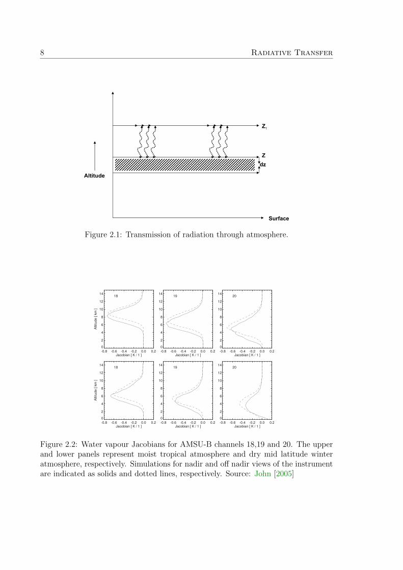
ARTS can also simulate the Jacobians for temperature and trace gas concentra-tions, which is generally defined as the partial derivative of radiance with respectto atmospheric parameters influencing it. The straight forward way to evaluate thisquantity is the use of perturbation method where radiances are simulated for a refer-ence state vector and re-determined successively through small perturbations in eachelement of the state vector. This procedure is time consuming due to which ARTScalculates this analytically [Buehler et al., 2005a]. For example, the humidity Jaco-bians simulated by ARTS for three different channels of AMSU-B is shown in Figure2.2

8 Radiative Transfer

dz

Z1

Surface

Altitude

Z

Figure 2.1: Transmission of radiation through atmosphere.

-0.8 -0.6 -0.4 -0.2 0.0 0.2Jacobian [ K / 1 ]

0

2

4

6

8

10

12

14

Altitude [ k

m ]

18

-0.8 -0.6 -0.4 -0.2 0.0 0.2Jacobian [ K / 1 ]

0

2

4

6

8

10

12

1419

-0.8 -0.6 -0.4 -0.2 0.0 0.2Jacobian [ K / 1 ]

0

2

4

6

8

10

12

1420

-0.8 -0.6 -0.4 -0.2 0.0 0.2Jacobian [ K / 1 ]

0

2

4

6

8

10

12

14

Altitude [ k

m ]

18

-0.8 -0.6 -0.4 -0.2 0.0 0.2Jacobian [ K / 1 ]

0

2

4

6

8

10

12

1419

-0.8 -0.6 -0.4 -0.2 0.0 0.2Jacobian [ K / 1 ]

0

2

4

6

8

10

12

1420

Figure 2.2: Water vapour Jacobians for AMSU-B channels 18,19 and 20. The upperand lower panels represent moist tropical atmosphere and dry mid latitude winteratmosphere, respectively. Simulations for nadir and off nadir views of the instrumentare indicated as solids and dotted lines, respectively. Source: John [2005]

Chapter 3

Humidity Retrieval Method

The measurements from space platforms are ideal in gaining a better understanding ofglobal distribution of atmospheric humidity. The meteorological satellites capable ofmeasuring atmospheric humidity do so by sensing the radiation emitted from differentparts of the Earth’s atmosphere. Satellite measurements, therefore do not providedirect measurements of humidity. Rather, they provide a radiance intensity which isa function of atmospheric constituents. Retrieval methods aid in getting the requiredinformation from the radiance measured by satellites. This chapter discusses a non-linear method for retrieval of humidity which forms the basis of the paper I enclosedin the thesis. This method is based on data clustering and fuzzy logic. Althoughthe paper demonstrates in detail the merits of the retrieval method over conventionalmethods in terms of accuracy, the very basic fundamental information have not beencovered. The present chapter aims to furnish certain background information on re-trieval methods which could help in better comprehension of the perspective of thepaper. The detailed mathematical formulations however have been exempted.

3.1 Fuzzy Logic

Fuzzy logic is a problem-solving enabled mathematical concept, inspired from real lifesituations [Zadeh, 1965]. The real situations in human interactions are not centredwholly on an all or nothing alternative but somewhere between the both. While acomputer is programmed to solve a problem through a binary approach of zeroes andones where it has to take a yes or no decision, the fuzzy logic technique employs fuzzylogic variables that can be assigned a value between 0 and 1. The added advantage isthat it can deal with non mathematical, linguistic variables such as which dominatehuman thought processes and communications. These linguistic variables are definedthrough IF-THEN statements and a host of other operators.

A fuzzy set is defined as a set without a crisp, clearly defined boundary and is anextension of classical sets. If X is a universal set and its elements are denoted by x,

9

10 Humidity Retrieval Method

then fuzzy set A in X is defined as the set of ordered pair

A = {x, µA (x) |x ⊂ X} (3.1)

where µA (x) is called membership function which maps universal set X to the realinterval [0 1]. The closer µA (x) is to 1 the more is the chance of x belonging to A.µA (x) gives the degree of membership to x in A. The set-theoretic operations of union,intersection and complement for fuzzy sets are defined through membership functions.Let A and B denote the pair of fuzzy set in X with membership functions µA (x) andµB (x) respectively. The membership function of union and the membership functionof intersection are defined as [Kaufmann, 1975]:

µA∪B = max (µA (x) , µB (x)) (3.2)

µA∩B = min (µA (x) , µB (x)) (3.3)

Complement of fuzzy set A is defined as µA (x) = 1− µA (x)The retrieval using fuzzy logic is enabled by formulating conditional statements

using IF and THEN statements. Linguistic rules that describe a system consists of twoparts; a premise part (between the IF and THEN) and a consequent block (followingTHEN). The approach to a problem using fuzzy logic is facilitated through fuzzyinference systems (FIS). The fuzzy reasoning mechanisms adopted in fuzzy inferencesystems are as follows: The first step is the fuzzification of the input which is aprocess of assigning membership value to each input using an appropriate membershipfunction. In the present context input refers to the satellite sounder measurements.Fuzzification is the process of classifying the input into different value ranges, or moreprecisely, it is a process of assigning a linguistic label (small, medium and large) tothe input as shown in Figure 3.1. Linguist variables, as the name implies are non-numerical variables that are used to define the rules in fuzzy logic. For example,the height of a person is a linguistic variable which can assume the values such as’tall’ or ’short’. The ’tall’ or ’short’ attribute is referred to as linguistic label. Thesecond step is to combine different rules generated by fuzzy rule base to get thefiring strength of each rule. The concept of firing strength is explained here withthe help of Figure 3.2. The Figure 3.2 shows A1, A2, B1 and B2 as linguistic labelsassigned to the inputs which when combined using appropriate fuzzy operators (ANDor OR) produces weights (w1 or w2) or firing strength. The third step is to make theconsequent of each rule depending on the firing strength.

The different steps of fuzzy reasoning are shown in Figure 3.2. The FIS usesdifferent types of fuzzy reasonings and the one used in the paper has been proposedby Takagi and Sugeno [1985] where the output of each rule is a linear combinationof input variables plus a constant term, and the final output is the weighted averageof each rule’s output. This is depicted in the type 3 of the consequent part of theFigure 3.2. Hereafter this FIS architecture will be referred to as TS model. Forexample, a fuzzy rule using TS model can be written as, IF x is A1 and y is B1

THEN f1 = p1x1 + q1x1 + r1, where A1 and B1 are linguistic labels.

3.1. Fuzzy Logic 11

Figure 3.1: Classification of input into different value ranges and assigning of mem-bership values.

C2

C1

C2

C1

(or min)

consequent partpremise part

type 3type 2type 1

averageweighted

averageweighted

w1*z1+w2*z2

w1+w2=z

w1

z2=px+qy+r

z1=ax+by+c

z (centroid of area)

max

w2

Z

Z

w1

w2

X

X

Y

Y

z1

z2

A1 B1

A2 B2

multiplication

w1*z1+w2*z2

w1+w2=z

Z

Z

x y

Figure 2: Commonly used fuzzy if-then rules and fuzzy reasoning mechanisms.

Figure 3.2: Various steps of Fuzzy reasoning mechanism adopted in FIS. Source:Shing and Jang [1993]


3.2 Data Clustering Methods

Data clustering technique is essentially a numerical method of classification, and as itsname indicates, seeks application where a large group of data needs to be partitionedinto certain nearly homogeneous classes. It is a common statistical tool finding usein almost all branches of science. Therefore, though the ultimate task is to have aclassified data, the methods employed to attain it could be different depending onthe nature of the dataset. There are different types of clusterings and depending onthe application, clusters can vary. Cluster analysis includes a wide range of statisticaltechniques with the most common approaches to finding clusters being distance based,centroid based,or density based [S.Aldenderfer and Blashfield].

The main idea behind clustering methods is to find out a cluster center, which isan indicator of where the heart of each cluster is located. Most popular algorithmsin use determine clusters in the dataset by minimizing a cost function of Euclideandistance. Among these, one of the widely used algorithms is hard-c means algorithm(HCM) [Mcqueen, 1967, Hartigan and Wong, 1979]. The HCM algorithm tries tominimize the cost function of the form:

J =c∑

i=1

(n∑

k=1

||Xk − ci||2)

(3.4)

where c is the total number of clusters and the cost function is based on Euclideandistance between a vector Xk and the corresponding cluster centre ci. The clustersformed as a result of classification are defined by a binary characteristic matrix, Malso called the membership matrix Mik where Mik is 1 if kth data point Xk belongsto cluster i and 0 otherwise.

The fuzzified c-means (FCM) is another popular clustering algorithm which clas-sifies data into clusters in such a way that each data point is not bound exclusivelyto any particular cluster but can associate to all the clusters specified by a mem-bership grade [Jang et al., 1997]. This characteristic of assigning membership valuesdistinguishes FCM from HCM. Fuzzy partitioning is achieved in FCM by allowingthe membership to take all values between 0 and 1. The objective function which isto be minimized is the generalization of Equation 3.4.

J =c∑

i=1

(n∑

k=1

Mik||Xk − ci||2)

(3.5)

where Mik is the membership matrix which can take the values between 0 and 1.The FCM and HCM algorithms start by randomly assigning a guess for the initialcluster centre. The cluster centres and membership grades are updated in successiveiterations.

Since the number of clusters is specified initially for both FCM and HCM, theycome under the category of supervised algorithms. Conversely, if the number ofclusters are not known, then unsupervised algorithms are employed. Subtractive

3.3. ANFIS 13

clustering belongs to the category of unsupervised algorithm and is based on thedensity of data points in the feature space [Chiu, 1994]. In subtractive clusteringeach data point is the possible candidate for the cluster centre. A density measure ateach data point is defined as

Di =n∑

j=1

exp

(||xi − xj||2(

ra2

)2

)(3.6)

where ra is a positive constant representing neighbourhood radius. A data point willhave a high density value if it has many neighboring data points. The first clustercentre Xc1 is chosen as the point having maximum density value Dc1 . In the nextstep, the density value of each data point will be revised as follows:

Di = Di −Dc1 exp

(||xi − xc1||2(

rb2

)2

)(3.7)

This process will exclude the selected cluster centre as the candidate for the nextcluster, as the first cluster centre, Xc1 will have significantly reduced density measure.After revising the density function, the next cluster centre is selected as the pointhaving the greatest density. Sufficient number of clusters can be obtained by contin-uing this process. The clustering method which is used in the paper is subtractiveclustering and using this method the dataset is clustered prior to application of fuzzyrules as explained in the previous section.

3.3 ANFIS

ANFIS stands for adaptive neuron-fuzzy inference systems. In ANFIS an adaptivenetwork has been included to fine tune the fuzzy rule base generated by TS modelShing and Jang [1993]. An adaptive network, like a neural network has nodes andconnecting links through which nodes are connected. The nodes are called adaptive,which means that the output of these nodes depend on the parameter pertaining tothis node, and the rules are learned by changing these parameters.

ANFIS has five layers and each has its own dedicated function. In ANFIS theparameters associated with first and last node have been changed during its trainingphase. The first layer has a node function which is either bell shaped,

µAi (x) =1

1 +[(

x−ciai

)]bi (3.8)

or Gaussian shaped

µAi (x) = exp

[−(x− ciai

)2]

(3.9)


where x is the input to the node i, and Ai is the linguistic label (small, large, mediumetc) associated with this node function. The parameter set {ai, bi, ci} ({ci, ai}) con-tains the premise parameters and as the values of these parameters change, it changesthe shape of the membership function. The output node has the parameter set{pi, qi, ri} and the output can be written as the linear combination of these parame-ters. These parameters are called consequent parameters.

In ANFIS a hybrid algorithm is used to change the consequent and premise pa-rameters using a set of training dataset. The premise parameters are changed usinggradient descent method which tries to minimize an error function of the form:

E =∑

p

Ep (3.10)

where Ep is the error in the pth training datset which is the difference in original andANFIS output and is a function of premise and consequent parameters. For exampleif α is the parameter of the input node (premise parameter) then the update formulafor α is

∆α = −η∂E∂α

(3.11)

where η is the learning rate. This method can also be applied to update the con-sequent parameters but the method is generally slow and likely to be trapped inlocal minima. Therefore in ANFIS a least square method is applied to change theconsequent parameters. As mentioned earlier the output of the ANFIS is a linearcombination of premise parameters which makes it possible to make an equation ofthe form AX=B using N training dataset for given values of premise parameters. Xis the unknown vector whose elements are consequent parameters. A least squaremethod can be used to find X by minimizing the squared error ||AX −B||2.

3.3. ANFIS 15

y

y

2

1

2

1

2

1

2

1

layer 5

layer 4

layer 3layer 2

layer 1

yx

yxB

B

A

A

f2w2

1w 1f

w2

1w

w2

1wx

f

X

X

Y

Y

A B

A B

x

1w

w2

1f

f2

= p x +q y +r

= p x +q y +r =

w2w1

2w 2ff1w1 +

2w 2ff1w1f = +

+

(a)

(b)

2

1

2

1

2

1

Figure 4: (a) Type-3 fuzzy reasoning; (b) equivalent ANFIS (type-3 ANFIS).i Oi "Ai !x"$x i AiOi Aix Ai "Ai!x""Ai !x" # $!x ciai " %bi $"Ai!x" exp$ !x ciai " %$fai bi cig fai cigAi wi "Ai!x" # "Bi!y"$ i $ -i iwi wiw # w $ i $ -

Figure 3.3: TS model fuzzy reasoning having two fuzzy rules (a) and the equivalentANFIS architecture (b). Source: Shing and Jang [1993]

Chapter 4

Radiosonde Corrections

This chapter presents an overview of various types of correction applied on VaisalaRS92 radiosonde humidity measurements. Vaisala radiosondes are the most widelyused radiosondes in the world. Though radiosondes are the vital sources of informa-tion on atmospheric humidity distribution, its data quality in the upper troposphereis known to be poor [Elliott and Gaffen, 1991, Moradi et al., 2010, Miloshevich et al.,2009, Soden and Lanzante, 1996]. These data quality issues may arise from sev-eral factors. Incorrect calibration of the humidity sensors, error caused due to solarheating of the humidity sensors and a slow sensor response at low temperatures aresome of the most plausible reasons. Several studies have highlighted these errors andhave introduced various correction methods [Vomel et al., 2007, Turner et al., 2003,Miloshevich et al., 2001], but none of the studies so far have actually depicted theimportance of correction through comparison with satellite measurements which isthe main topic of the second paper. The corrections applied on the radiosondes arebased on the work by Miloshevich et al. [2009]. This chapter has been written with anaim of furnishing the reader with a general idea of the radiosonde correction methodswhich could not be covered in detail in the article.

4.1 Radiosonde Correction Methods

The basis of the correction is the removal of bias in the Vaisala RS92 radiosondehumidity measurements through a comparison with three reference instruments ofknown accuracy. These instruments are cryogenic frost-point hygrometer which isintended for correction above 700 hPa, a microwave radiometer for lower troposphere,and a system of 6 calibrated RH probes for the surface. Mean calibration biases inRS92 humidity measurements were determined by comparing the RS92 measurementswith simultaneous measurements from these instruments and thereafter these biaseswere removed. The correction is a function of pressure (P) and relative humidity(RH) and is given by

17

18 Radiosonde Corrections

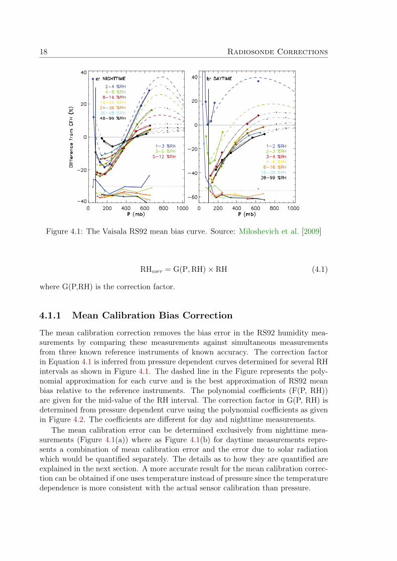
Figure 4.1: The Vaisala RS92 mean bias curve. Source: Miloshevich et al. [2009]

RHcorr = G(P,RH)× RH (4.1)

where G(P,RH) is the correction factor.

4.1.1 Mean Calibration Bias Correction

The mean calibration correction removes the bias error in the RS92 humidity mea-surements by comparing these measurements against simultaneous measurementsfrom three known reference instruments of known accuracy. The correction factorin Equation 4.1 is inferred from pressure dependent curves determined for several RHintervals as shown in Figure 4.1. The dashed line in the Figure represents the poly-nomial approximation for each curve and is the best approximation of RS92 meanbias relative to the reference instruments. The polynomial coefficients (F(P, RH))are given for the mid-value of the RH interval. The correction factor in G(P, RH) isdetermined from pressure dependent curve using the polynomial coefficients as givenin Figure 4.2. The coefficients are different for day and nighttime measurements.

The mean calibration error can be determined exclusively from nighttime mea-surements (Figure 4.1(a)) where as Figure 4.1(b) for daytime measurements repre-sents a combination of mean calibration error and the error due to solar radiationwhich would be quantified separately. The details as to how they are quantified areexplained in the next section. A more accurate result for the mean calibration correc-tion can be obtained if one uses temperature instead of pressure since the temperaturedependence is more consistent with the actual sensor calibration than pressure.

4.1. Radiosonde Correction Methods 19

RH or Fit

Coefficients

a0 a1 a2 a3 a4 a5 a6

Nightb

�1.5 5.1993e+1 ÿ7.9576eÿ1 3.9051eÿ3 ÿ8.9666eÿ6 1.1825eÿ8 ÿ8.4134eÿ12 2.4210eÿ152.5 4.3729e+1 ÿ7.8757eÿ1 3.8100eÿ3 ÿ8.4919eÿ6 1.0830eÿ8 ÿ7.5247eÿ12 2.1433eÿ153 1.0102e+1 ÿ3.5020eÿ1 1.3771eÿ3 ÿ1.8918eÿ6 1.5448eÿ9 ÿ1.0460eÿ12 3.7543eÿ164 ÿ1.2053e+1 ÿ1.3963eÿ1 5.0608eÿ4 8.7142eÿ8 ÿ1.1580eÿ9 9.6029eÿ13 ÿ2.2738eÿ166 ÿ1.9292e+1 ÿ5.3081eÿ2 1.1776eÿ5 1.5888eÿ6 ÿ3.7721eÿ9 3.2351eÿ12 ÿ9.7876eÿ168.5 ÿ1.4220e+1 ÿ1.5629eÿ1 7.3102eÿ4 ÿ5.7830eÿ7 ÿ6.9512eÿ10 1.1583eÿ12 ÿ4.3573eÿ1612 ÿ8.6609e+0 ÿ2.3153eÿ1 1.1601eÿ3 ÿ1.6559eÿ6 4.7114eÿ10 6.4842eÿ13 ÿ3.7600eÿ1620 ÿ1.2075e+1 ÿ9.0493eÿ2 4.5730eÿ4 ÿ4.4334eÿ7 ÿ2.5251eÿ10 5.6512eÿ13 ÿ2.1830eÿ1630 ÿ8.4463e+0 ÿ6.7739eÿ2 2.1850eÿ4 2.4128eÿ7 ÿ1.1680eÿ9 1.1593eÿ12 ÿ3.6948eÿ1642 ÿ7.5226e+0 ÿ9.4287eÿ2 5.6012eÿ4 ÿ1.0285eÿ6 8.1621eÿ10 ÿ2.4513eÿ13 3.3189eÿ18�50 3.7854e+1 ÿ4.9026eÿ1 2.0313eÿ3 ÿ3.9299eÿ6 3.9439eÿ9 ÿ1.9776eÿ12 3.8808eÿ16for P < P2 4.3867e+3 ÿ3.7335e+2 1.2676e+1 ÿ1.9717eÿ1 1.1628eÿ3

Dayc

0 6.8793e+0 1.6275eÿ1 ÿ3.2097eÿ5 ÿ4.1883eÿ7 5.0829eÿ10 ÿ1.9028eÿ131.9 ÿ1.3058e+1 1.5405eÿ1 3.0599eÿ5 ÿ4.9033eÿ7 5.4030eÿ10 ÿ1.9315eÿ132.4 ÿ4.7161e+1 1.3916eÿ1 1.3784eÿ4 ÿ6.1264eÿ7 5.9504eÿ10 ÿ1.9805eÿ133.5 ÿ6.0069e+1 1.3320eÿ1 1.8078eÿ4 ÿ6.6256eÿ7 6.1467eÿ10 ÿ1.9661eÿ135 ÿ6.6681e+1 1.4741eÿ1 1.6426eÿ5 ÿ1.4146eÿ7 8.9222eÿ12 4.0390eÿ1411 ÿ6.7112e+1 1.1009eÿ1 3.7366eÿ4 ÿ1.2284eÿ6 1.2520eÿ9 ÿ4.3857eÿ1322 ÿ6.6938e+1 1.1812eÿ1 2.8349eÿ4 ÿ1.0166eÿ6 1.0377eÿ9 ÿ3.5797eÿ13�34 ÿ6.0024e+1 1.4726eÿ1 ÿ6.9462eÿ5 ÿ2.0216eÿ7 3.1579eÿ10 ÿ1.3450eÿ13for P < P2 5.4021e+3 ÿ3.5312e+2 8.1766e+0 ÿ6.4838eÿ2SF(a) 9.6886eÿ1 3.3717eÿ3 ÿ4.2343eÿ5 1.7882eÿ7frac SRE(a) ÿ1.6061eÿ3 3.7746eÿ2 ÿ4.7402eÿ4 2.0018eÿ6

a

Figure 4.2: Polynomial coefficients provided for mean bias correction for day andnighttime RS 92 radiosonde profiles. Source: Miloshevich et al. [2009]

4.1.2 Solar Radiation Error Correction

In addition to the correction for mean calibration error, the daytime radiosonde mea-surements need to be corrected for solar radiation error which is caused due to solarheating of RH sensors [Vomel et al., 2007]. The solar radiation error (SRE) is pri-marily a function of incident solar flux which in turn is a function of solar altitudeangle. If the solar altitude angle is high then SRE in the radiosonde will be higherdue to enhanced heating of the RH sensor. The Figure 4.1(b) shows the mean calibra-tion bias curve of RS92 sensor determined during daytime sounding. The polynomialcoefficients (F(P, RH, 66 ◦)) for daytime soundings are also given in Figure 4.2 andare provided for a higher solar altitude angle (66◦). These coefficients represent acombination of mean calibration error and the SRE.

The SRE component of the daytime mean bias is the difference between daytimeand nighttime mean biases (SRE(66◦) =F(P, RH, 66◦)-F(P, RH, night)). The SREcomponent in daytime dataset for other solar altitude angles can be obtained bymultiplying SRE(66◦) with the necessary SRE fraction which can be determined fromFigure 4.3 by using the polynomial fit given in Figure 4.2 (frac SRE(α)). Thus, SREfor any solar altitude angle α is given by

SRE(α) = SRE(66◦)× fraction(α) (4.2)

Once the SRE for a particular solar angle is obtained, the coefficients for daytimemeasurements can be obtained by adding the SRE(α) to F (P, RH, night).

F (P,RH, day) = SRE(α) + F (P,RH, night) (4.3)

In brief, the daytime correction for Vaisala RS92 radiosonde consists of correctionfor mean calibartion error (SRE=0) and the correction for SRE.


Figure 4.3: Solar fraction error as the function of solar altitude angle. Source: Milo-shevich et al. [2009]

4.1.3 Time Lag Correction

The time lag error is the result of a slow sensor response to changes in the ambienthumidity at low temperatures (<-45 °C) prevalent usually in the upper troposphereand the lower stratosphere. The time lag error affects the sensor’s ability to discern thedetailed vertical structure of humidity profile, thus yielding a smooth and incorrectRH profile. The time lag error can be corrected, provided that the sensor timeconstant and the vertical humidity gradient information are known [Miloshevich et al.,2004]. The time constant (τ) refers to the time required for the sensor to respondto 63% of an instantaneous change in the ambient humidity and is a function oftemperature. This value is usually determined in the laboratory. The time constantfor RS92 sensor as a function of temperature is shown in Figure 4.4.

The ambient humidity can be obtained from the measured humidity using theformula

Ua = U + τ(T )× dU

dt(4.4)

4.1. Radiosonde Correction Methods 21

Figure 4.4: RS92 time constant as a function of temperature. Source: http://

milo-scientific.com/prof/radiosonde.php.

where dUdt

is the local humidity gradient, Ua is the ambient humidity and U is themeasured humidity. The time constant τ is given by

τ(T ) = 0.8× exp(−0.7399 +−0.07718× T ) (4.5)

The time lag correction is based on the assumption that the ambient humidity re-mains almost constant for a short interval of the measurement time. This necessitatesthe requirement of a very good temporal resolution for the profiles. It is also neces-sary that the relative humidity values in the profiles must have precision to certaindecimal values in order that the correction may be effective.

http://milo-scientific.com/prof/radiosonde.php

http://milo-scientific.com/prof/radiosonde.php

Chapter 5

Diurnal cycle of humidity

Microwave observations of humidity from NOAA satellites were made possiblewith the deployment of Advanced Microwave Sounding Unit (AMSU-B) sensor inthe year 1998. In the present context of climate studies, the requirement of longterm homogeneous data is largely a necessity. The AMSU data obtained from thedifferent NOAA satellites are usually composited to get a long term dataset. However,these data are not homogeneous due to factors like changes in spectral characteristics,sensor degradation and drift in the satellite orbit.

Orbital parameters of polar orbiting, sun-synchronous satellites are designed insuch way that they measure the radiation emitted from any point on the Earth andits atmosphere at similar local times, thus sampling the same part of the diurnal cycleof the geophysical parameters measured. However, in reality, factors like atmosphericdrag, the Earth’s non-spherical shape, the gravitational pull from celestial bodies andsolar activity causes the orbit to drift towards the centre of the Earth [John et al.,2011b]. Such a drift in orbital height obviously would lead to changes in the orbitingperiod and hence a change in the local sampling time of the satellites leading toundesirable aliasing of diurnal cycle into the time series data from polar orbiters.

The drift in the satellite dataset can be corrected provided we have knowledge ofthe diurnal behaviour of the measurements. In this study, our aim is to constructa diurnal behaviour of brightness temperatures obtained from microwave humiditysounder measurements by combining data from different NOAA satellite platforms.Microwave data have the advantage of having an all-sky sampling as compared toonly clear-sky sampling for infrared measurements [John et al., 2011a]. The diurnalcycle has been constructed following the approach of Anders et al. [2011] for HIRSmeasurements which is described in the following sections.

5.1 Data

The data used in the study is from AMSU-B and microwave humidity sounder (MHS)sensors on-board NOAA satellites. AMSU-B is flown on NOAA satellite-15, 16 and 17

23

24 Diurnal cycle of humidity

Equator Crossing Time for NOAA/MetOp POES

1999 2000 2001 2002 2003 2004 2005 2006 2007 2008 2009 2010 2011Time [ years ]

14

16

18

20

22Local T

ime [ h

our

]

NOAA-15

NOAA-16

NOAA-17

NOAA-18

MetOpA

NOAA-19

Figure 5.1: Temporal span and equator crossing time of NOAA satellites for ascendingorbit. Source: John et al. [2011b]

and MHS is on NOAA-18. They are both 5 channel microwave radiometers dedicatedto measuring atmospheric humidity, an important climate variable [Held and Soden,2000], but not very well simulated by current climate models [John and Soden, 2007].Out of the five channels, three (18, 19, 20) are placed near a strong water absorptionline at 183 GHz. The channels 16 and 17, at 89 GHZ and 150 GHz respectively lookdeeper through the atmosphere on to the Earth’s surface. All the five channels are notidentical for MHS and AMSU-B and the differences are in channels 17 and 20 [Johnet al., 2011b]. Both AMSU-B and MHS sensors are cross track scanning instrumentshaving 90 Earth field-of-views per scan line.

We have used the data spanning the years 2000-2010 taken from 4 different satel-lites, the NOAA-15, 16, 17 and 18 satellites. With the exception of NOAA 15, datafrom the other satellites do not have the full temporal coverage from 2000-2010 asshown in Table 5.1. The measurements from each satellite for ascending and descend-ing orbits for each day were gridded as 2.5◦ X 2.5◦ latitude-longitude grid points. Thusa single grid point would have multiple data from different satellites for different lo-cal times. Each grid point was then composited on a monthly basis over the periodfrom 2000–2010. The near nadir observations alone have been used to avoid anyuncertainty due to limb correction and scan asymmetry [Buehler et al., 2005b].

5.2 Construction of Diurnal cycle

As can be seen from the Figure 5.1 the equatorial crossing times for the satellitesespecially NOAA-15 and 16, have drifted over time. For example, the equatorialoverpass time of NOAA 16 has drifted approximately by around 5 hours over a periodof 10 years. Drifts of varying magnitudes are observed in other satellites too. Thisdrift can cause false trends in the time series [Jacobowitz et al., 2003]. On the otherhand, this drift has an obvious advantage in that it facilitates a better means ofextracting the diurnal behaviour of brightness temperature. A diurnal cycle has beenfitted for each grid point separately for each month using a second order Fourierseries.

5.3. Results 25

Table 5.1: Data time period of different NOAA satellites.

Satellite Time periodNOAA-15 2000-2010NOAA-16 2001-2010NOAA-17 2003-2010NOAA-18 2006-2010

Tb = a0 + a1cosπ(t− t1)

12+ a2cos

2π(t− t2)

12(5.1)

where Tb is the brightness temperature, t is the observational local time in hours,a0 is the mean value of Tb, a1 is the half peak to peak amplitude of the 24 hourlyoscillation, a2 is the half peak to peak amplitude of the 12 hourly oscillation and t1and t2 are phase. After expanding Equation 5.1 can be written as

Tb = b0 + b1cos

(πt

12

)+ b2sin

(πt

12

)+ b3cos

(2πt

12

)+ b4sin

(2πt

12

)(5.2)

The coeffcients b0, b1, b2 b3 and b4 are determined using linear regression. Using thesecoefficients amplitudes a0 to a2 and the phase t1 and t2 are determined.

A Monte Carlo error analysis has been performed to determine the uncertainty ofthe derived fit parameters (amplitudes a1 and a2 ) from the Fourier series. Measure-ments in each grid point would comprise of data from the different satellites with eachsatellite having different number of observations for their ascending and descendingpasses. Within a grid point, the data from each satellite for a particular pass con-taining say, ’n’ observations would then be replaced by a randomly generated datasethaving a similar mean and standard deviation as that of the ’n’ observations. Therandom numbers are generated using a normal distribution. Each grid point wouldthus have randomly generated data for each satellite for their ascending and descend-ing passes respectively. The fit parameters a1 and a2 were determined using Equation5.1. The process of randomizing the grid point data is repeated 300 times, thus gen-erating an equal numbers of fit parameters (a1 and a2). The standard deviation ofa1 and a2 thus generated is the uncertainty of the amplitudes. If this uncertaintyexceeds the original amplitude then the fit can not be accepted as real. In order thatthe fit be a valid one, we set the ratio of amplitude to standard deviation (signal tonoise ratio) to greater than 1.

5.3 Results

The results presented in this section mainly focus on the analysis of brightness tem-perature diurnal variations of channel 16. The channel 16 is a window channel located


in the microwave region and it senses mostly the Earth’s surface, so under clear skyconditions, the variations in this channel are expected to reflect the variations in thesurface temperature.

The amplitudes a1 and a2 of the diurnal variation of Channel 16 brightness tem-perature determined using the method described in section 5.2 are represented on amap for the months January and July (Figure 5.3). The amplitude a2 is significantlylower than that of a1 over most of the regions. The amplitude of diurnal variation islargest over land and lower over oceanic regions which is consistent with Anders et al.[2011]. Dry land regions exhibit maximum diurnal variation in amplitude a1 whichreaches over 10 K. Seasonal variation of the diurnal amplitude is clearly visible inthe map wherein the regions of Central America, Sahara desert, the Middle East andIndo-Pak regions exhibit a notable seasonal variation. Over most of the regions inAfrica, a strong diurnal variation in a1 is visible often exeeding 6 K. A strong diurnalvariation is observed over some parts of Antarctic region in the January map and asimilar variation in amplitude can be seen over the Arctic in July map. This may bedue to the large emissivity variation occurring due to the solar heating of the surfacewhich causes larger diurnal variation in channel 16 brightness temperature.

As explained in section 5.2 a Monte Carlo error analysis has been performed tofind the uncertainties in amplitude a1 and a2. The result is shown in Figure 5.4which maps the signal to noise ratio, therefore a larger magnitude of the ratio impliesa robust fit for the diurnal cycle. The map shows that the diurnal variations aresignificant over most of the land regions and is insignificant over most of the oceanicregions. The diurnal peak time of channel 16 brightness temperature for the monthsJanuary and July is shown in Figure 5.5. It is shown over those regions where thediurnal fit has been found to be significant from the Monte Carlo error analysis (signalto noise ratio > 1). Since the diurnal amplitude of these regions is dominated by thatof 24 hour oscillation (a1), the peak time shown here represents the peak time of 24hour oscillation. Over most of the land regions, the diurnal peak occurs after noon(12 pm) local time. This result is consistent considering that the maximum landtemperature due to solar heating occurs 2-3 hours before sunset. Exceptions howeverare seen over some of the oceanic regions and some regions of Arctic and Antarcticwhere the peak time is in the early morning.

5.4 Future Work

The main aim of constructing a diurnal cycle is to correct the drift in satellite mea-surements so as to generate a homogeneous long term climate dataset. The resultsshown in the previous section are preliminary. Prior to compositing the satellite mea-surements for creating the diurnal cycle, it is necessary to correct for inter-satellitebiases. Inter-satellite bias calculation has not been implemented in this study. There-fore, the immediate step would be to correct the inter-satellite biases based on themethod developed by John et al. [2011b]. Subsequent to construction of diurnal cy-cle from inter-satellite bias corrected dataset, the measurements will be corrected for

5.4. Future Work 27

0 6 12 18 24250

260

270

280

Local Time (hr)

Tb

16 [K

]

0 6 12 18 24250

260

270

280

290

Local Time (hr)

Tb

17 [K

]

0 6 12 18 24240

250

260

270

Local Time (hr)

Tb

18 [K

] 0 6 12 18 24

250

260

270

280

Local Time (hr)

Tb

19 [K

]

0 6 12 18 24250

260

270

280

290

Local Time (hr)

Tb

20 [K

]

NOAA15NOAA16NOAA17NOAA18

Figure 5.2: The diurnal variation in brightness temperature of channels 16–20 of aparticular grid point (31.25◦N, 1.25◦E) over Sahara desert. Black curve representsthe diurnal fit.

the drift and its impact would be studied by analysing the time-series against theuncorrected dataset.


Figure 5.3: The diurnal amplitudes a1 (left panel) and a2 (right panel) for the monthsJanuary (upper panels) and July (lower panels) for AMSU-B channel 16 . Unit ofamplitude is in Kelvin.

Figure 5.4: The uncertainty of the amplitudes a1 (left panel) and a2 (right panel)for the months January (upper panels) and July (lower panels). The uncertainty isdefined as the ratio of amplitude to its standard deviation. Unit is dimensionless.The white regions in the map indicate areas with misssing data.

5.4. Future Work 29

Figure 5.5: The diurnal local peak times in hours for the months January (left) andJuly (right). The white regions in the map indicate areas with misssing areas.

Chapter 6

Summary of Papers

This thesis encloses two papers related to study of atmospheric humidity. Themeasurements of atmospheric humidity are made available from two main sources,the radiosondes and the satellites. Though an accurate representation of humiditycan be obtained from radiosondes, its upper tropospheric humidity measurements areunreliable. On the other hand, measurements from satellites aid in getting globalinformation on atmospheric humidity. However, the accuracy of humidity retrievalfrom satellite measurements largely depends on how well an algorithm takes intoaccount the nonlinearity between satellite measurements and the atmospheric state.The paper I enclosed in the thesis deals with a retrieval method which could improvethe humidity retrieval accuracy from satellite measurements and paper II investigatesthe impact of various radiosonde humidity corrections in the upper troposphere bycomparing them with satellite measurements.

6.1 Paper I

This paper introduces a non linear retrieval method based on data clustering andfuzzy logic for the retrieval of humidity from satellite infrared sounder measurements.Simulated Geostationary Operational Environmental (GOES) infrared sounder mea-surements have been used in this study. The advantage of the present method over theconventional retrieval methods such as linear or nonlinear regression retrieval meth-ods has been demonstrated. The data clustering prior to the application of fuzzy rulefor the retrieval is proved to be very effective in improving the retrieval accuracy. Ithas been shown that the present method reduces the root mean square by 20% inhumidity retrieval as compared to non linear regression method. For improving theretrieval accuracy using linear (or non linear) regression methods, the regression co-efficient has to be determined separately for each latitude zone. Since, in the presentstudy, the data clustering has already been applied prior to application of fuzzy rules,the regional classification is already taken into account in the retrieval method. Thisprovides an advantage for this method to yield a better retrieval accuracy even if the

31

32 Summary of Papers

algorithm is trained with a global training dataset.

6.2 Paper II

This paper mainly demonstrates the importance of radiosonde humidity correctionsfor satellite validation. In this paper various correction methods have been applied tothe radiosonde humidity measurements which were then compared with satellite mea-surements both in infrared and microwave spectral range. This correction has beenapplied to daytime and nighttime datasets separately. The major correction whichis required for the nighttime dataset is the bias removal associated with calibrationerror in the measurement where as for daytime soundings, major source of correctionis due to solar radiation error. The application of this correction is shown to bevery important for improving the accuracy of satellite estimate of upper troposherichumidity. After application of this correction, the agreement between the radiosondeand the satellite measurements for daytime and nighttime could be brought down to acomparable level. This study also cautions against the use of uncorrected radiosondemeasurements for satellite validation.

References

V. L. Anders, I. A. Mackenzie, S. F. B. Tett, and L. Shi. Climatological diurnal cyclesin clear-sky brightness temperatures from the high-resolution infrared radiationsounder (hirs). J. Atmos. Oceanic Technol., 28:1199–1205, 2011. doi: 10.1175/JTECH-D-11-00093.1.

S. A. Buehler and V. O. John. A simple method to relate microwave radiances toupper tropospheric humidity. J. Geophys. Res., 110:D02110, 2005. doi: 10.1029/2004JD005111.

S. A. Buehler, P. Eriksson, T. Kuhn, A. von Engeln, and C. Verdes. ARTS, theatmospheric radiative transfer simulator. J. Quant. Spectrosc. Radiat. Transfer, 91(1):65–93, Feb. 2005a. doi: 10.1016/j.jqsrt.2004.05.051.

S. A. Buehler, M. Kuvatov, and V. O. John. Scan asymmetries in AMSU-B data.Geophys. Res. Lett., 32:L24810, 2005b. doi: 10.1029/2005GL024747.

S. A. Buehler, M. Kuvatov, V. O. John, M. Milz, B. J. Soden, D. L. Jackson, andJ. Notholt. An upper tropospheric humidity data set from operational satellitemicrowave data. J. Geophys. Res., 113:D14110, 2008. doi: 10.1029/2007JD009314.

S. A. Buehler, V. O. John, A. Kottayil, M. Milz, and P. Eriksson. Efficient radiativetransfer simulations for a broadband infrared radiometer — combining a weightedmean of representative frequencies approach with frequency selection by simulatedannealing. J. Quant. Spectrosc. Radiat. Transfer, 111(4):602–615, Mar. 2010. doi:10.1016/j.jqsrt.2009.10.018.

S. A. Buehler, P. Eriksson, and O. Lemke. Absorption lookup tables in the radiativetransfer model arts. J. Quant. Spectrosc. Radiat. Transfer, 112(10):1559–1567,2011. doi: 10.1016/j.jqsrt.2011.03.008.

S. Chiu. Fuzzy model identification based on cluster estimation. J. of Intelligent andFuzzy Systems, 2:267–278, 1994.

33

34 References

I. Durre, C. N. Williams, X. Yin, and R. S. Vose. Radiosonde-based trends in pre-cipitable water over the Northern Hemisphere: An update. Journal of GeophysicalResearch (Atmospheres), 114:D05112, Mar. 2009. doi: 10.1029/2008JD010989.

W. P. Elliott and D. J. Gaffen. On the utility of radiosonde humidity archives forclimate studies. Bull. Amer. Met. Soc., 72(10):1507–1520, 1991.

P. Eriksson, S. A. Buehler, C. P. Davis, C. Emde, and O. Lemke. ARTS, the at-mospheric radiative transfer simulator, version 2. J. Quant. Spectrosc. Radiat.Transfer, 112(10):1551–1558, 2011. doi: 10.1016/j.jqsrt.2011.03.001.

E. J. Fetzer, W. G. Read, D. Waliser, B. H. Kahn, B. Tian, H. Vomel, F. W. Irion,H. Su, A. Eldering, M. T. Juarez, J. Jiang, and V. Dang. Comparison of uppertropospheric water vapor observations from the microwave limb sounder and atmo-spheric infrared sounder. J. Geophys. Res., 113, 2008. doi: 10.1029/2008JD010000.

J. A. Hartigan and M. A. Wong. A k-means clustering algorithm. Applied Statistics,28:100–108, 1979.

I. M. Held and B. J. Soden. Water vapor feedback and global warming. Annu. Rev.Energy Environ., 25:441–475, 2000.

G. Holl, S. A. Buehler, J. Mendrok, and A. Kottayil. Simulating cloudy thermalinfrared radiances with an optimised frequency grid in the radiative transfer modelARTS. J. Quant. Spectrosc. Radiat. Transfer, to be submitted.

H. Jacobowitz, L. L. Stowe, G. Ohring, A. Heidinger, K. Knapp, and N. R. Nalli. TheAdvanced Very High Resolution Radiometer Pathfinder Atmosphere (PATMOS)Climate Dataset: A Resource for Climate Research. Bulletin of the AmericanMeteorological Society, 84:785–793, June 2003. doi: 10.1175/BAMS-84-6-785.

J. S. R. Jang, C. T. Sun, and E. Mizutani, editors. Neuro-fuzzy and soft computing: acomputational approach to learning and machine intelligence. Prentice Hall, 1997.

V. O. John. Analysis of upper tropospheric humidity measurements by microwavesounders and radiosondes. Berichte aus dem Institut fuer Umweltphysik. LogosVerlag Berlin, Apr. 2005. Ph. D. Thesis, University of Bremen, ISBN 3-8325-1010-9.

V. O. John and B. J. Soden. Temperature and humidity biases in global climatemodels and their impact on climate feedbacks. Geophys. Res. Lett., 34:L18704,2007. doi: 10.1029/2007GL030429.

V. O. John, G. Holl, R. P. Allan, S. A. Buehler, D. E. Parker, and B. J. Soden.Clear-sky biases in satellite infra-red estimates of upper tropospheric humidity andits trends. J. Geophys. Res., 116:D14108, 2011a. doi: 10.1029/2010JD015355.

References 35

V. O. John, G. Holl, S. A. Buehler, B. Candy, R. W. Saunders, and D. E. Parker.Understanding inter-satellite biases of microwave humidity sounders using globalSNOs. J. Geophys. Res., 2011b. in press.

A. Kaufmann, editor. Introduction to the theory of fuzzy sets. Academic Press,Newyork, 1975.

J. T. Kiehl and B. P. Briegleb. Comparison of the observed and calculated clear skygreenhouse effect: Implications for climate studies. J. Geophys. Res., 97(D9), 1992.doi: 10.1029/92JD00729.

A. Kottayil, P. K. Thapliyal, M. V. Shukla, P. K. Pal, P. C. Joshi, and R. R. Naval-gund. A new technique for temperature and humidity profile retrieval from infraredsounder observations using adaptive neuro-fuzzy inference system. IEEE Geosci.R. S., 48:1650 –1659, 2010. doi: 10.1109/TGRS.2009.2037314.

A. Kottayil, S. A. Buehler, V. O. John, L. M. Miloshevich, M. Milz, and G. Holl.On the importance of Vaisala RS92 radiosonde humidity corrections for a betteragreement between measured and modeled satellite radiances. J. Atmos. OceanicTechnol., 2011. doi: 10.1175/JTECH-D-11-00080.1. in press.

J. R. Lanzante and G. E. Gahrs. The ”clear-sky bias” of TOVS upper-tropospherichumidity. J. Climate, 13:4034–4041, 2000.

S. Manabe and R. T. Wetherald. Thermal Equilibrium of the Atmosphere with aGiven Distribution of Relative Humidity. Journal of Atmospheric Sciences, 24:241–259, May 1967. doi: 10.1175/1520-0469(1967)024〈0241:TEOTAW〉2.0.CO;2.

J. Mcqueen. Some methods for classification and analysis of multivariate observations.In Fifth Berkeley Symposium on Mathematical Statistics and Probability, pages 281–297, 1967.

L. M. Miloshevich, H. Vomel, A. Paukkunen, A. J. Heymsfield, and S. J. Oltmans.Characterization and correction of relative humidity measurements from vaisalaRS80-A radiosondes at cold temperatures. J. Atmos. Oceanic Technol., 18(2):135–156, 2001. doi: 10.1175/1520-0426(2001)018〈0135:CACORH〉2.0.CO;2.

L. M. Miloshevich, A. Paukkunen, H. Vomel, and S. J. Oltmans. Development andvalidation of a time-lag correction for Vaisala radiosonde humidity measurement.J. Atmos. Oceanic Technol., 21:1305–1327, 2004. doi: 10.1175/1520-0426(2004)021〈1305:DAVOAT〉2.0.CO;2.

L. M. Miloshevich, H. Vomel, D. N. Whiteman, and T. Leblanc. Accuracy assessmentand correction of vaisala RS92 radiosonde water vapor measurements. J. Geophys.Res., 114:D11305, 2009. ISSN 0148-0227. doi: 10.1029/2008JD011565.

36 References

I. Moradi, S. A. Buehler, V. O. John, and S. Eliasson. Comparing upper tropospherichumidity data from microwave satellite instruments and tropical radiosondes. J.Geophys. Res., 115:D24310, 2010. doi: 10.1029/2010JD013962.

P. P. Peixoto and A. H. Oort, editors. PHYSICS OF CLIMATE. Springer-VerlagNewyork, Inc., 1992.

R. T. Pierrehumbert, H. Brogniez, and R. Roca, editors. The Global Circu lationof the Atmosphere, chap. On the Relative Humidity of the Atmosphere. Princeton,2006.

W. G. Rees. Physical Principles of Remote Sensing. Cambridge university press, 2edition, 2001. ISBN 978-0-521-66948-1.

C. D. Rodgers, editor. INVERSE METHODS FOR ATMOSPHERIC SOUNDING.World Scientific Publishing Co.Pte.Ltd, 2000.

P. W. Rosenkranz. Water vapor microwave continuum absorption: A comparisonof measurements and models. Radio Sci., 33(4):919–928, 1998. (correction in 34,1025, 1999), ftp://mesa.mit.edu/phil/lbl_rt.

M. S.Aldenderfer and R. K. Blashfield, editors. Cluster Analysis, volume 44. SAGAPublication, Inc.

J. Schmetz, P. Pili, S. Tjemkes, D. Just, J. Kerkmann, S. Rota, and A. Ratier. Anintroduction to meteosat second generation (MSG). Bull. Amer. Met. Soc., 83(7):977–992, 2002.

S. C. Sherwood, R. Roca, T. M. Weckwerth, and N. G. Andronova. Troposphericwater vapor, convection, and climate. Rev. Geophys., 48:RG2001, 2010. doi: 10.1029/2009RG000301.

J. Shing and R. Jang. Adaptive-network-based fuzzy inference system. IEEE Trans.Syst., Man, Cybern., 23:665–685, 1993.

B. J. Soden and F. P. Bretherton. Upper tropospheric relative humidity from theGOES 6.7 µm channel: Method and climatology for july 1987. J. Geophys. Res.,98(D9):16,669–16,688, 1993.

B. J. Soden and J. R. Lanzante. An assessment of satellite and radiosonde climatolo-gies of upper-tropospheric water vapor. J. Climate, 9:1235–1250, 1996.

B. J. Soden, D. J. Jackson, V. Ramaswamy, M. D. Schwarzkopf, and X. Huang. Theradiative signature of upper tropospheric moistening. Science, 310(5749):841–844,Nov. 2005. doi: 10.1126/science.1115602.

T. Takagi and M. Sugeno. Fuzzy identification of systems and its applications tomodeling and control. IEEE Trans. Syst., Man, Cybern., 15:116–132, 1985.

ftp://mesa.mit.edu/phil/lbl_rt

References 37

P. K. Thapliyal, M. V. Shukla, S. Shah, P. K. Pal, P. C. Joshi, and A. Kottayil.An algorithm for the estimation of upper tropospheric humidity from kalpana ob-servations: Methodology and validation. J. Geophys. Res., 116:1–16, 2011. doi:10.1029/2010JD014291.

K. E. Trenberth, J. Fasullo, and L. Smith. Trends and variability in column-integratedatmospheric water vapor. Climate Dynamics, 24:741–758, 2005.

D. D. Turner, B. M. Lesht, S. A. Clough, J. C. Liljegren, H. E. Revercomb, andD. C. Tobin. Dry bias and variability in vaisala RS80-H radiosondes: The ARMexperience. J. Atmos. Oceanic Technol., 20:117–132, 2003.

H. Vomel, H. Selkirk, L. Miloshevich, J. Valverde-Canossa, J. Valdes, E. Kyroe,R. Kivi, W. Stolz, G. Peng, and J. A. Diaz. Radiation dry bias of the VaisalaRS92 humidity sensor. J. Atmos. Oceanic Technol., 24(6):953–963, 2007. doi:10.1175/JTECH2019.1.

F. J. Wentz, L. Ricciardulli, K. Hilburn, and C. Mears. How much more rain willglobal warming bring? Science, 317:233–235, 2007. doi: 10.1126/science.1140746.

L. A. Zadeh. Fuzzy sets. Inf. Control, 8:338–353, 1965.

38 References

Paper I

A new technique for temperatureand humidity profile retrieval from

infrared sounder observations usingAdaptive Neuro-Fuzzy Inference

System

Authors:A. Kottayil, P. K. Thapliyal, M. V. Shukla, P. K. Pal, P. C. Joshi and R. R. Naval-gund

Bibliography:A. Kottayil, P. K. Thapliyal, M. V. Shukla, P. K. Pal, P. C. Joshi, and R. R. Naval-gund. A new technique for temperature and humidity profile retrieval from infraredsounder observations using adaptive neuro-fuzzy inference system. IEEE Geosci. R.S., 48:1650 –1659, 2010. doi: 10.1109/TGRS.2009.2037314

39

1650 IEEE TRANSACTIONS ON GEOSCIENCE AND REMOTE SENSING, VOL. 48, NO. 4, APRIL 2010

A New Technique for Temperature and HumidityProfile Retrieval From Infrared-Sounder

Observations Using the Adaptive Neuro-FuzzyInference System

Kottayil S. Ajil, Pradeep Kumar Thapliyal, Munn V. Shukla, Pradip K. Pal,Prakash C. Joshi, and Ranganath R. Navalgund

Abstract—The accuracy of the atmospheric profiles of tempera-ture and humidity, retrieved from infrared-sounder observationsusing physical retrieval algorithms, depends directly on the qualityof the first-guess profiles. In the past, forecasts from the numerical-weather-prediction models were extensively used as the first guess.During the past few years, the first guess for physical retrieval isbeing estimated using regression techniques from sounder observ-ations. In this study, a new nonlinear technique has been describedto improve the first guess using simulated infrared brightness tem-peratures for GOES-12 Sounder channels. The present techniqueuses fuzzy logic and data clustering to establish a relationshipbetween simulated sounder observations and atmospheric pro-files. This relationship is further strengthened using the Adap-tive Neuro-Fuzzy Inference System (ANFIS) by fine-tuning theexisting fuzzy-rule base. The results of ANFIS retrieval have beencompared with those from the nonlinear (polynomial) regressionretrieval. It has been found that ANFIS is more robust and reducesroot mean squared error by 20% in humidity profile retrievalcompared with the nonlinear regression technique. In addition, ithas been shown that the ANFIS technique has an added advantageof its global application without any need for classification of thetraining data that is required in the regression techniques.

Index Terms—Atmospheric profiles, fuzzy inference system(FIS), fuzzy neural networks, infrared sounder.

I. INTRODUCTION

SATELLITE-DERIVED atmospheric parameters play amajor role in the improvement of numerical weather pre-

diction (NWP) at various timescales. Infrared-sounder obser-vations from polar and geostationary platforms have provideda wealth of 3-D atmospheric data of temperature and hu-midity, particularly over oceanic regions, which is otherwisevery difficult to obtain using limited radiosonde observations.Various sounding instruments have been developed so far,e.g., the High-resolution InfraRed Sounder (HIRS) onboard theNational Oceanic and Atmospheric Administration (NOAA)

Manuscript received December 2, 2008; revised April 27, 2009 andAugust 24, 2009. First published January 22, 2010; current version publishedMarch 24, 2010.

K. S. Ajil is with the Department of Space Science, Lulea TechnicalUniversity, 971 87 Lulea, Sweden (e-mail: [email protected]).

P. K. Thapliyal, M. V. Shukla, P. K. Pal, P. C. Joshi, and R. R. Navalgundare with the Space Applications Center, Indian Space Research Organisation,Ahmedabad 380 015, India (e-mail: [email protected]; [email protected]; [email protected]; [email protected];[email protected]; [email protected]).

Digital Object Identifier 10.1109/TGRS.2009.2037314

polar-orbiting satellite, the Atmospheric InfraRed Sounder(AIRS) onboard the Earth Observing System Aqua satellite, theInfrared Atmospheric Sounding Interferometer (IASI) onboardthe METOP satellite, the Sounder onboard the GeostationaryOperational Environmental Satellite (GOES), and the ModerateResolution Imaging Spectroradiometer (MODIS) onboard theTerra and Aqua satellites. India is planning to launch INSAT-3D in a geostationary orbit with an 18-channel infrared sounder(plus a visible channel for the daytime cloud detection) on-board, for continuous coverage of the Indian ocean region,which is, so far, available only from GOES over the U.S. region.

The retrieval of atmospheric temperature and humidity pro-files from a finite number of sounder observations is an ill-posed as well as an ill-conditioned problem. Various algorithmshave been developed to invert the sounding observations to ob-tain atmospheric profiles. Linear-regression-based algorithmshave been developed by Smith and Woolf [1] for Nimbus-6HIRS, Goldberg et al. [2] and Weisz et al. [3] for AIRS,and Seemann et al. [4] for MODIS. Physical retrieval algo-rithms have been developed by Smith and Woolf [5], Smith[6], Hayden [7], Ma et al. [8], Li et al. [9], Susskind et al.[10], etc., for various satellite sounders. Physical retrieval usesforecast atmospheric profiles from NWP models as the firstguess. However, the state-of-the-art physical retrieval algo-rithms use atmospheric profiles from regression retrieval asthe first guess [4], [9], [11], [12]. An advantage of using firstguess from regression retrieval is that these atmospheric profilesare physically consistent with the sounder observations. Manynonlinear statistical algorithms have also been developed forprofile retrieval using artificial neural networks (ANNs) fordifferent types of infrared and microwave sounding instruments[13]–[16]. An ANN is a derivative-based approach, which triesto minimize a cost function by adjusting the weights inter-connecting the neurons. The problem with the ANN approachis that it can be very easily trapped in local minima, givingthe false impression of network training. Fuzzy logic, used inthis paper, on the other hand, uses basic human perception forsolving the problem by formulating linguistic rules which canbe very easily interpreted.

Linearization of sounder observations with respect to theatmospheric states is very important in regression retrieval, par-ticularly for humidity retrieval, because satellite brightness tem-perature observations have highly nonlinear dependence on theatmospheric water vapor content. Contrary to this, atmospheric

0196-2892/$26.00 © 2010 IEEE

Authorized licensed use limited to: LULEA TEKNISKA UNIVERSITET. Downloaded on March 29,2010 at 05:01:36 EDT from IEEE Xplore. Restrictions apply.

AJIL et al.: NEW TECHNIQUE FOR TEMPERATURE AND HUMIDITY PROFILE RETRIEVAL 1651

temperature profiles have a linear relationship with the sounder-observed brightness temperatures. Due to this reason, althoughthe retrieval of atmospheric profiles from infrared-soundermeasurements can give better temperature retrieval accuracy,humidity retrieval accuracy is not up to the appreciable level. Inthis paper, an attempt has been made to develop a new nonlineartechnique to retrieve temperature and humidity profiles that willbest serve the purpose of providing an improved first guessto the physical retrieval algorithms. The nonlinear algorithmdeveloped in this paper is primarily based on the integrationof fuzzy logic and the data clustering techniques.

The retrieval using the present method consists of two parts.In the first part, the technique of data clustering (CLUST) hasbeen applied to classify the output (temperature and humidityprofiles at different atmospheric levels) depending on its homo-geneity. Following data classification, fuzzy rules are applied toestablish a relationship between inputs (sounder measurements)and the clustered data set. Details are included in Section III-A.In the second part, the input (membership functions) and theoutput parameters are fine-tuned using an adaptive network, andthis is realized through the Adaptive Neuro-Fuzzy InferenceSystem (ANFIS). In other words, the network fine-tunes theexisting fuzzy-rule base determined in the first part. The ANFIStraining is equivalent to that of an ordinary neural network, butmorphologically, it is different. A hybrid algorithm is employedto fine-tune the fuzzy-rule base through linear least square andgradient descent method and is described in Section III-A2.Algorithms have been developed separately for both parts toenable the profile retrieval, and the details of the same aredescribed in Section IV.

II. DATA SET AND RADIATIVE TRANSFER MODEL

To demonstrate the performance of the nonlinear techniquedeveloped in this paper, we have used the simulated data set ofthe GOES-12 Sounder channels using the fast radiative transfermodel RTTOV-7 [17]–[19] developed at the European Centerfor Medium Range Weather Forecasting (ECMWF). RTTOV-7 uses the Pressure Layer Optical Depth algorithm [20] forradiative transfer calculation. Radiance calculations are doneat 43 pressure levels ranging from 1013 to 0.1 hPa, takinginto account the observational zenith angle and the absorptionby well-mixed gases, water vapor, and ozone. The GOES-12Sounder consists of 18 infrared spectral bands ranging from 3.7to 14.7 μm. These channels are sensitive to atmospheric gases,primarily CO2, O3, and H2O (Table I), that detect radiationemanating from different levels of atmosphere. This enablesthe measurement of the vertical distribution of temperature,moisture, and ozone. Out of the 18 infrared channels, only15 were used in this paper, excluding the ozone absorptionchannel (Channel#9) and the shortwave infrared channels, asthey are contaminated by reflected solar radiation (Channel#17and 18). The radiative transfer calculations for the GOES-12sounder have been performed using RTTOV-7, generating anensemble of simulated brightness temperatures along with theactual atmospheric states. Clear-sky radiances, simulated fornadir looking observations (zenith angle = 0◦), have been usedin this paper. In order to account for the measurement noise,a Gaussian-distributed random number with zero mean andstandard deviation σ has been added to the simulated radi-ances. σ includes instrument noise and forward model error:

TABLE IGOES-12 SOUNDER CHANNEL SPECIFICATIONS

σ =√

e2j + f2

j , where ej is the instrument noise (Table I) and

fj is the forward model error of channel “j.” The constant valueof fj = 0.2 K has been used in this paper.

Sounder channel brightness temperatures are simulated forthe SeeBor data set (version 4, University of Wisconsin [21])comprising of ∼15 000 diverse global profiles of temperature,humidity, and ozone from the Thermodynamic Initial GuessRetrieval data set (TIGR3), NOAA data set (NOAA88), andECMWF analysis data sets. TIGR3 and NOAA88 data setsare diverse profiles of atmosphere collected from various ra-diosonde observations. The retrieval algorithms are trainedwith two different data sets: regional data set covering thearea 30S–30N, 0–180E and global data set covering the area80S–80N, 180W–180E. The numbers of training profiles usedfor the regional and global retrievals are 2026 and 9167, respec-tively, which comprise profiles from the SeeBor data set ex-cluding NOAA88 profiles. Simulated brightness temperaturesfor the NOAA88 data set (∼1200 profiles) covering the region(30S–30N, 0–180E) have been used for testing the algorithm.The effect of the regional and global training data sets inretrieving the profiles using nonlinear regression and ANFISis discussed in Section IV.

III. RETRIEVAL METHODOLOGY

This section describes the methodology of data clustering(CLUST) and ANFIS for the retrieval of temperature and hu-midity profiles using simulated infrared-sounder observations.The results of retrieval using CLUST and ANFIS have beencompared with the nonlinear regression technique (REGRE)



that is widely used as the first guess to the physical retrieval.These techniques are described in the following sections.

A. Fuzzy Logic

Fuzzy-set theory [22] was born out of the realization that theworld that surrounds us is defined by a nondistinct boundary.It is a mathematical tool to deal with the linguistic variables,i.e., the concept described in natural language. Fuzzy sets andfuzzy operators are the basic building blocks of fuzzy logic.Linguistic rules that describe a system consist of two blocks:an antecedent (premise) block and a consequent block. The ap-proach to a problem using fuzzy logic is facilitated through FIS.Fuzzy inference is a process, which helps in the formulation ofa mapping from a given input to an output using fuzzy logic.The process of fuzzy inference involves membership functions,a fuzzy logic operator, and IF–THEN rules. The fuzzificationlayer in FIS generates membership values for all the inputsthrough membership functions which lie in the premise part.This process is often known as fuzzification. A fuzzy logiccontroller in FIS combines all the membership values on thepremise part to get the firing strength (weight). The next step isthe generation of qualified consequents for each rule dependingon the firing strength that is aggregated to produce a crispoutput. This step is called defuzzification.

1) Data Clustering (CLUST): Data clustering, by definition,is the grouping of the data into similar categories andidentifying natural groupings of data from a large data set. Dataclustering can be performed using supervised or unsupervisedlearning. The fuzzified c-means algorithm [23] is a supervisedalgorithm because a priori knowledge of a number of clusters isrequired. If the number of clusters is not known beforehand, itis necessary to apply unsupervised algorithms. In unsupervisedlearning, algorithms are provided with just data points and nolabels; the task is to find out a suitable representation of theunderlying distribution of data. In this paper, we have used sub-tractive clustering that belongs to the category of unsupervisedalgorithms and is based on the density of data points in thefeature space [23]. Here, brightness temperatures from sounderchannels have been used as data points for clustering. The aimis to find a region in the feature space with a high density ofdata points. Consider a collection of K data points (size oftraining data set) specified by n-dimensional vectors (numberof sounder channels) uk, k = 1, 2, . . . , n, which are assumed tobe normalized. Since each data point is a candidate for a clustercenter, a density measure at the data point uk is defined as

Dk =

K∑

j=1

exp

(−‖uk − uj‖

(ra/2)2

)(1)

where ra is a positive constant. A data point will have a highdensity value if it has many neighboring data points. Only thefuzzy neighborhood within the radius ra contributes to thedensity measure.

After calculating the density measure for each data point, thepoint with the highest density is selected as the first cluster cen-ter. Let ucl be the point selected and Dcl be its density measure.Next, the density measure for each data point ucl is revised by

Dk = Dk − Dcl

K∑

j=1

exp

(−‖uk − uj‖

(rb/2)2

)(2)

where rb is a positive constant. Therefore, the data pointsnear the first cluster center ucl will have significantly reduceddensity measures, making the points unlikely to be selected asthe next cluster center. The constant rb defines a neighborhoodto be reduced in density measure. It is normally larger than ra

to prevent closely spaced cluster centers; typically, rb = 1.5ra.The data points within the selected cluster are removed(subtracted) to ensure their absence in the next cluster. Thealgorithm looks for a new point with the highest numberof neighbors. This is continued until all the data points areevaluated.

The first part of the retrieval algorithm is realized by formu-lating a FIS through data clustering. In the first step, subtractiveclustering algorithm is applied to the brightness temperaturesas input and the humidity and temperature at each atmosphericlevel as output. The subtractive clustering algorithm dividesthe data points at each atmospheric level into a number ofclusters, which, in turn, gives the same number of rules fordesired parameters (temperature and humidity) at that particularatmospheric level. More precisely, it is categorizing the entiredata set into different clusters depending on the characteristicvariability of the atmospheric states, which are observed indifferent regions of the globe. For example, there is a widedifference in the range of humidity values found in the tropicsand in the polar region. The clustering algorithm takes intoaccount this variability while doing the clustering. The numberof clusters generated using subtractive clustering depends onthe search radius, which is the Euclidean distance between thecluster center and the data point. A small search radius willhave more number of clusters and vice versa. In the presentalgorithm, the search radius of 0.4 is found to be sufficient forall the levels. It should be noted that there must be a tradeoffbetween the search radius and the desired retrieval accuracy.One can choose this depending on how the variability of thedata set under consideration fluctuates. The premise part of thefuzzy rule has brightness temperatures whereas the consequentpart has a clustered data set. The advantage of data clusteringprior to the application of fuzzy rules is that rules can be devisedseparately for different regions. The input values are gradedbetween 0 and 1 and are coded in the form of fuzzy membershipfunctions. In the present algorithm, we have used a Gaussian-shaped membership function to represent the input. Takagi andSugeno’s fuzzy rules are used [28], in which the output of eachrule is a linear combination of the input variables in additionto a constant term. The final output is the weighted average ofeach rule’s output. The weight is the firing strength which isobtained by combining the membership values on the premisepart of each rule through a specific T-norm operator, usuallymultiplication or minimum.

Fuzzy rules were generated using the training data set. Usingthe regional training data set with a search radius of 0.4, wehave four data clusters for humidity in the lower levels andfive in a few of the upper levels. The same numbers of clustershave been generated using the global training data set with asearch radius of 0.4. Similarly, for temperature, we have fourclusters for all the retrieved levels. The numbers of fuzzy rulesvary depending on the total number of clusters. Separate FISswere devised for each atmospheric level. This part of the FIShas been generated using the standard MATLAB routine genfis2available in the fuzzy logic toolbox.



Fig. 1. Schematic diagram of ANFIS for two inputs (x1 and x2) and oneoutput with the two fuzzy rules (A1 and A2 for input x1, and B1 and B2 forinput x2) of Takagi and Sugeno type (α1 and α2 are firing strengths, and f1

and f2 are outputs from different rules).

2) ANFIS: System identification is the process of determin-ing a mathematical model of an unknown system by observingits input–output data. Some of the commonly used techniquesfor nonlinear system identification include fuzzy logic [28],[29], neural network [30], genetic algorithm, etc. A neuro-fuzzysystem [23], [24] combines the fuzzy logic and an adaptivenetwork so as to integrate human expert knowledge and thelearning capability. The generated FIS through the subtractiveclustering algorithm has been trained using ANFIS [32]. AN-FIS is a method of tuning the existing fuzzy-rule base with alearning algorithm using a collection of training data sets. Thisallows the rule base to adapt. The ANFIS architecture is func-tionally equivalent to a fuzzy-rule base similar to Takagi andSugeno’s [25] which has five layers. Fig. 1 shows a schematicdiagram of ANFIS for a simple case having two inputs, twofuzzy IF–THEN rules, and one output. Here, A1, A2, B1, andB2 are the linguistic labels, e.g., small, medium, large, etc., as-sociated with the inputs coded in the form of fuzzy membershipfunctions. This procedure facilitates the classification of theinput values.

The output membership function of the node i of layer 1,which is generally a Gaussian function, is given by

μAi(xi) = exp

[−

(xi − ci

ai

)2]

(3)

where xi is the input (sounder channels’ Tb) to node i andAi is the linguistic label associated with this node function.The values of the parameter set {ai, ci} determine the shape ofthe Gaussian function. The parameters in this layer are calledpremise parameters. Generally, continuous and piecewise dif-ferentiable functions (trapezoidal/triangular membership func-tions) are the possible candidates for the node function in thislayer. The inputs are mapped into the membership functionsthrough (3). The task of the second layer in the ANFIS is tocombine the output values from node 1 so as to get the firingstrength for each rule. Each node output represents the firingstrength αi of the ith rule. The function that can perform ageneralized AND operation can be used as the node functionin this layer. Every node in layer 3 is a fixed node which is thenormalized firing strength (αi), given by

αi =αi∑i

αi. (4)

Layer 4 is an adaptive node in which the network calculates thenode output as a linear combination of inputs

αi · fi = αi · (pi · x1 + qi · x2 + · · · + ri) (5)

where fi is the output of the ith rule and {pi, qi, . . . , ri}is the parameter set of this node. The parameters in thislayer are called consequent parameters. A hybrid algorithm inANFIS updates the consequent and premise parameters througha learning procedure having two parts. In the first part, the entiretraining patterns are propagated, and the optimal consequentparameters are estimated by an iterative least mean squareprocedure, while the premise parameters are assumed to befixed. In the second part, patterns are propagated again, andin this epoch, backpropagation gradient descent method [26]is used to modify the premise parameters, while the consequentparameters remain fixed. These techniques provide a methodto learn information about a data set, by computing the mem-bership function parameters that best allow the associated FISto track the given input/output data. The parameters associ-ated with the membership functions will change through thelearning process. The computation of these parameters (or theiradjustment) is facilitated by a gradient vector, which providesa measure of how well the FIS is modeling the input/outputdata for a given set of parameters. This learning method workssimilarly to that of neural networks [31]. The readers may referto [32] for a comprehensive understanding of the mathematicaldetails of ANFIS.

In this paper, the utility “anfis” available in the MATLABfuzzy logic toolbox has been used for the fine-tuning of thefuzzy-rule base generated by subtractive clustering.

B. Nonlinear Regression (REGRE)

Ill-posed and ill-conditioned problems, arising in the retrievalof the atmospheric profiles of temperature and humidity fromsounder observations, are usually solved by the least squarelinear regression method [1], [4], [27]. If the atmospheric statevector is represented by X and measurements by Y , thenthe linear relation between these may be expressed by thefollowing:

X = CY T (6)

where C is the matrix of regression coefficients. If the di-mension of X is “m” (number of outputs) and that of Y is“n” (number of inputs), then the dimension of C is “m × n.”Superscript “T” denotes the transpose of the matrix. In thepresent regression procedure, the primary inputs are the bright-ness temperatures of 15 GOES Sounder channels and thesurface pressure. The quadratic terms of the sounder brightnesstemperatures are also used as additional inputs to make itnonlinear (or polynomial) regression to account for the non-linearity of atmospheric humidity in relation to the Sounderobservations. The least square solution of (6) to compute C isgiven by the following:

C = XY (Y TY )−1. (7)

Regression methods use a statistical relationship between thecollocated data set of sounder-measured radiances and simul-taneously observed atmospheric profiles of temperature andhumidity from radiosonde. Perfectly collocated matchup data



Fig. 2. Block diagrams summarize the retrieval procedure. The letter T stands for temperature, and q is for humidity.

sets are very difficult to obtain due to various constraints, suchas the spatial resolution difference, observation time difference,presence of clouds, errors in radiosonde measurements, etc. Inthis paper, the matchup data set to compute regression coef-ficients is generated from the simulated GOES-12 brightnesstemperatures and the corresponding atmospheric profiles.

The detailed methodology of retrieval using the aforemen-tioned three methods: CLUST, ANFIS, and REGRE have beenshown schematically in Fig. 2 for better understanding. Twosets of coefficients have been generated for each of these meth-ods: 1) CLUST_GLO, ANFIS_GLO, and REGRE_GLO usingthe global training data set and 2) CLUST_REG, ANFIS_REG,and REGRE_REG using the regional training data set.

These coefficients have been applied on the brightness tem-peratures in the independent regional testing data set to retrievethe atmospheric profiles of temperature and humidity. Retrievalstatistics has been computed in terms of the root mean squarederror (rmse), the mean bias (BIAS), and the coefficient ofcorrelation (R).

IV. RESULTS AND DISCUSSIONS

Fig. 3 shows the rmse of the retrieved humidity profiles usingregional and global coefficients for all the three retrieval tech-niques, namely, REGRE, CLUST, and ANFIS. In general, rmsedecreases from the surface level to upper atmospheric levels.



Fig. 3. RMSEs of the humidity retrieval using (solid line) regional and(dashed line) global coefficients for three different retrieval techniques:REGRE, CLUST, and ANFIS.

Fig. 4. Mean bias of the humidity retrieval using (solid line) regionaland (dashed line) global coefficients for three different retrieval techniques:REGRE, CLUST, and ANFIS.

This is due to the fact that the absolute humidity values are largeat surface levels that decrease with the height. It is observedthat fuzzy-based methods (CLUST and ANFIS) provide muchbetter retrieval accuracy compared with the nonlinear regres-sion (REGRE), using both global and regional coefficients. Forregression retrieval, there is a large improvement in humidityretrieval when regional coefficients (REGRE_REG) are usedinstead of global coefficients (REGRE_GLO). RMSE in near-surface humidity retrieval in REGRE_REG is nearly 15%smaller compared with REGRE_GLO. Due to this reason, sepa-rate sets of coefficients are generated in regression retrieval fordifferent latitude zones. However, using CLUST and ANFIS,the results remain almost the same while using regional orglobal coefficients. There is more than 25% reduction in thermse of the humidity profile using the fuzzy-logic-based re-trieval technique compared with those from REGRE. It is in-teresting to note that, contrary to REGRE retrievals, the rmse inCLUST and ANFIS is slightly lower with global coefficientscompared with that with regional coefficients. This showsthe advantage of using fuzzy-logic- and data-clustering-basedalgorithms, as the data set is automatically categorized within

Fig. 5. Coefficient of correlation of the humidity retrieval using (solid line)regional and (dashed line) global coefficients for three different retrievaltechniques: REGRE, CLUST, and ANFIS.

Fig. 6. RMSE in the temperature profile retrieval with REGRE, CLUST, andANFIS retrieval techniques using regional coefficients.

the retrieval procedure based on fuzzy rules. Fig. 4 shows themean bias in humidity retrieval. It is clear from this figurethat the bias observed from CLUST and ANFIS are very smalland ranges between −0.3 and +0.2 g/kg, whereas it is morethan 1.0 g/kg at the lower atmospheric levels for REGRE thatdecreases in the upper atmospheric levels. In REGRE, the biasusing global coefficients is higher (∼1.5 g/kg) compared withthat using regional coefficients (∼1.0 g/kg), whereas above the800-hPa level, REGRE with regional coefficients has higherbias compared with the global coefficients. This large biasin REGRE may be attributed to the limited ability of thenonlinear regression method to pick up the nonlinearity in the“humidity–brightness-temperature relationship” as comparedwith the ANFIS. In nonlinear regression, we have includedonly a quadratic term (T 2

b ) to represent the nonlinearity inthe relationship, whereas in ANFIS, the nonlinearity is verywell represented by fuzzy rules. Fig. 5 shows the coefficientof correlation (R) between the actual and the retrieved humidi-ties at different atmospheric levels. It may be seen that R inREGRE_GLO is lowest at all levels ranging from 0.7 at thesurface to 0.85 at 400 hPa. Improvement in terms of R is largest(∼10%) at lower levels and smaller (∼2%) at higher levels. The



Fig. 7. Histogram of absolute error in humidity retrieval (in grams per kilogram) in REGRE and ANFIS for global and regional coefficients at differentatmospheric levels: (a) 1000, (b) 850, (c) 750, and (d) 600 hPa.

ANFIS_GLO-retrieved humidity has the highest R (> 0.80)followed closely by CLUST_GLO with the actual humidity atall atmospheric levels. This high degree of correlation of re-trieved and actual humidities using fuzzy techniques withglobal coefficients may be due to the fact that the global coeffi-cients use a larger data set than the regional coefficients, thushaving better resources for the data clustering. However, thesedifferences in the statistics using global and regional coeffi-cients are very small compared with those in the regressiontechnique.

It may be noted from Fig. 6 that there is a very smallimprovement in the temperature profile retrieval using ANFISand CLUST compared with REGRE. The highest improvementin temperature profile using ANFIS in the range of 0.3–0.5 K is noted around the tropopause region (100–200 hPa)which is less than 0.2 K at other levels. This may be due tothe linear relationship between the brightness temperature andthe temperature profile, thereby leaving very little scope ofimprovement in temperature profile retrieval using a nonlineartechnique. Contrary to this, large nonlinearity exists betweenatmospheric humidity and brightness temperature observations,hence providing enough scope of improvement in the humidityprofile retrieval using a suitable nonlinear technique. Thisnonlinearity is taken care of in the ANFIS retrieval for humidityin a better way compared with REGRE. It may also be notedfrom Figs. 3–5 that, out of the two fuzzy-based techniques,ANFIS shows improvement over CLUST. Therefore, ANFIS ischosen for further analysis and comparison with REGRE.

Fig. 7 shows the histogram of the absolute humidity errorin REGRE and ANFIS for different atmospheric levels 1000,850, 750, and 600 hPa. The total numbers of profiles for thesepressure levels are 712, 1206, 1227, and 1227, respectively.It is evident that the frequency of smaller absolute humidityerrors in ANFIS is considerably higher compared with REGRE,whereas the frequency of higher absolute humidity errors inANFIS is very small compared with the REGRE retrieval.For higher atmospheric levels, these differences in the fre-

quency become smaller. This shows that the improvement inthe humidity retrieval using ANFIS is very high in the loweratmosphere, whereas there is small improvement in the humid-ity profiles above 600 hPa as compared with REGRE. Fig. 7(a)shows that, for REGRE retrieval, there are only 20%–25% datapoints showing an absolute humidity retrieval error of less than1.0 g/kg, which is considerably high (33%) in the ANFIShumidity retrieval. Similarly, for absolute humidity errors(> 4 g/kg), there are 10% points in each category for REGRE,which is less than 5% for ANFIS retrieval. Similar features areobserved at other levels also, confirming the importance of theANFIS technique in reducing the magnitude of retrieval errors.

Figs. 8 and 9 show scatter plots of actual humidity withretrieved humidity using REGRE_REG and REGRE_GLO,respectively, at 1000-, 850-, 750-, and 600-hPa atmosphericlevels. It is observed that the scatter is small at lower humidityvalues and large toward higher humidity values. Scatter issmaller in the REGRE_REG compared with REGRE_GLO,particularly at higher humidity values, thus indicating the im-portance of regional classification in the nonlinear regressiontechnique. RMSE values for REGRE_REG are 2.97, 2.26,1.84, and 0.98 g/kg for 1000-, 850-, 750-, and 600-hPa lev-els, respectively, which are significantly on the higher sidein the case of global regression REGRE_GLO, i.e., 3.64,2.57, 2.04, and 1.21 g/kg, respectively. Similarly, Figs. 10and 11 show scatter plots of actual with retrieved humidityusing ANFIS_REG and ANFIS_GLO, respectively, at 1000-,850-, 750-, and 600-hPa atmospheric levels. It is encour-aging to see that the scatter between the actual and theretrieved humidities at all levels has reduced significantly,particularly for the higher values of humidity. RMSE valuesfor ANFIS_REG are 2.67, 1.94, 1.46, and 0.80 g/kg at 1000-,850-, 750-, and 600-hPa levels, respectively, which are sig-nificantly smaller than those from the regression retrieval. Ithas been observed that the rmse in ANFIS_GLO is slightlylower (2.59, 1.87, 1.40, and 0.76 g/kg, respectively) than thatfrom ANFIS_REG. This indicates that the use of more data in



Fig. 8. Scatter diagram of retrieved humidity (in grams per kilogram) versusactual humidity (in grams per kilogram) using REGRE_REG at differentatmospheric levels: (a) 1000, (b) 850, (c) 750, and (d) 600 hPa.

Fig. 9. Scatter diagram of retrieved humidity (in grams per kilogram) versusactual humidity (in grams per kilogram) using REGRE_GLO at differentatmospheric levels: (a) 1000, (b) 850, (c) 750, and (d) 600 hPa.

training using fuzzy method will aid to the data clustering andhence improve the fuzzy retrieval technique using global train-ing data.

Results from these analyses indicate the possibility of pro-viding better estimates of humidity profiles using the ANFISretrieval technique that can be used as the improved first guessfor nonlinear physical retrieval as compared with the first guessfrom the conventional regression (linear or nonlinear) retrieval.Apart from the accuracy, the time taken in generating the firstguess is very crucial. We found ANFIS to be fast enough inproviding the first guess to the physical retrieval procedure.

Fig. 10. Scatter diagram of retrieved humidity (in grams per kilogram)versus actual humidity (in grams per kilogram) using ANFIS_REG at differentatmospheric levels: (a) 1000, (b) 850, (c) 750, and (d) 600 hPa.

Fig. 11. Scatter diagram of retrieved humidity (in grams per kilogram)versus actual humidity (in grams per kilogram) using ANFIS_GLO at differentatmospheric levels: (a) 1000, (b) 850, (c) 750, and (d) 600 hPa.

The training time of ANFIS depends on the complexity of thenetwork, the total number of epochs, and the search radius.In this paper, the training time for 100 epochs with a searchradius of 0.4 is approximately 3 s for each parameter at eachatmospheric level. However, this being a one-time exercise, thetime taken in the training is not a constraint. For the retrieval,ANFIS works very fast and takes only 1.2 s for retrievingthe temperature and the humidity profile at 40 atmosphericlevels for ∼1200 testing data points on Intel computer having aPentium 4 processor (2.66 MHz) compared with ∼50 ms usingthe nonlinear regression technique.



V. CONCLUSION

In this paper, a new technique based on fuzzy logic hasbeen developed for the retrieval of atmospheric temperatureand humidity profiles using simulated infrared-sounder bright-ness temperatures, and its advantages have been demonstratedby comparison with a nonlinear regression technique. Twotechniques based on fuzzy logic, i.e., data clustering andANFIS, have been used to train the simulated training data fortemperature and humidity retrieval from the sounder-observedbrightness temperatures. Separate coefficients have been gen-erated for the global and regional training data sets. Statisticshas been generated by applying these coefficients on the in-dependent regional simulated data set. It has been observedthat the fuzzy-logic-based techniques significantly improvedthe humidity retrieval compared with the nonlinear regression.The improvement in humidity profile retrieval using a fuzzy-logic-based technique is more than 25% reduction in the rmsecompared with that with the nonlinear regression retrieval. Thepresent study also demonstrates that, while there is a need toclassify the training data in different latitude zones to improvethe retrieval accuracy in nonlinear regression retrieval, there isno such need in the case of fuzzy-logic-based techniques. It isalso observed that, out of the two fuzzy-logic-based techniques,ANFIS provides slightly better accuracy compared to that withCLUST. ANFIS retrieval using the global training data setprovides better humidity retrieval accuracies compared withthose obtained from the regional training data set.

Improvement in the humidity retrieval is required to makethis information suitable for assimilation in NWP and climatemodels. World Meteorological Organization requirements oftemperature and humidity accuracies for NWP are 1 K in thetroposphere for temperature and 15%–25% in the humiditymixing ratio. The present ANFIS retrieval algorithm is anattempt to provide improved estimates of humidity as an inputfirst guess to the nonlinear physical retrieval compared withthat provided by conventional linear or nonlinear regressiontechniques.

The application of the present technique to real satelliteobservations needs to be investigated in detail. This includesthe investigation of the sensitivity of different sensor noisespecifications on retrieval using satellite observations. The ex-tension of the present ANFIS technique to the hyperspectralsounder measurements, such as IASI and AIRS, needs spe-cial investigation. This may require the application of data-compression techniques, like the principal component analysis,for reducing the dimensionality of the input measurements. Thelarge number of inputs (2378 channels in AIRS and ∼8500channels in IASI) will require more fuzzy rules and will makethe ANFIS architecture more complicated, leading to increasedmemory space and retrieval time.

ACKNOWLEDGMENT

The authors would like to thank Dr. J. S. Parihar, the DeputyDirector of the Remote Sensing Applications Area, for theconstant encouragement and Dr. A. Huang and Dr. J. Li ofthe University of Wisconsin, for their useful discussions andguidance in the sounding retrieval. The authors would liketo thank three anonymous reviewers and the Associate Editorfor the valuable comments and suggestions that greatly helped

in improving the contents and the quality of this paper andDr. N. K. Vyas of SAC, ISRO, for critically going through themanuscript.

REFERENCES

[1] W. L. Smith and H. M. Woolf, “The use of eigenvectors of statisticalcovariance matrices for interpreting satellite sounding radiometer obser-vations,” J. Atmos. Sci., vol. 33, no. 7, pp. 1127–1140, Jul. 1976.

[2] M. D. Goldberg, Y. Qu, L. M. McMillin, W. Wolf, L. Zhou, andM. Divakarla, “AIRS near-real-time products and algorithms in support ofoperational numerical weather prediction,” IEEE Trans. Geosci. RemoteSens., vol. 41, no. 2, pp. 379–389, Feb. 2003.

[3] E. Weisz, H.-L. Huang, J. Li, E. Borbas, K. Baggett, P. K. Thapliyal,and L. Guan, “International MODIS and AIRS processing package: AIRSproducts and applications,” J. Appl. Remote Sens., vol. 1, no. 1, p. 013519,Jul. 2008, DOI: 10.1117/1.2766867.

[4] S. W. Seeman, J. Li, W. P. Menzel, and L. E. Gumley, “Operationalretrieval of atmospheric temperature, moisture, and ozone from MODISinfrared radiances,” J. Appl. Meteorol., vol. 42, no. 8, pp. 1072–1091,Aug. 2003.

[5] W. L. Smith and H. M. Woolf, “A linear simultaneous solution for temper-ature and absorbing constituent profiles from radiance spectra,” in Proc.4th Int. TOVS Study Conf. Tech., Igls, Austria, 1988, pp. 330–344.

[6] W. L. Smith, “The retrieval of atmospheric profiles from VAS geostation-ary radiance observations,” J. Atmos. Sci., vol. 40, no. 8, pp. 2025–2035,Aug. 1983.

[7] C. M. Hayden, “GOES-VAS simultaneous temperature–moisture retrievalalgorithm,” J. Appl. Meteorol., vol. 27, no. 6, pp. 705–733, Jun. 1988.

[8] X. L. Ma, T. Schmit, and W. Smith, “A non-linear physical retrievalalgorithm—Its application to the GOES-8/9 sounder,” J. Appl. Meteorol.,vol. 38, no. 5, pp. 501–503, May 1999.

[9] J. Li, W. W. Wolf, W. P. Menzel, W. Zhang, H. L. Huang, and T. H. Achtor,“Global sounding of the atmosphere from ATOVS measurements: Thealgorithm and validation,” J. Appl. Meteorol., vol. 39, no. 8, pp. 1248–1268, Aug. 2000.

[10] J. Susskind, C. D. Barnet, and J. M. Blaisdell, “Retrieval of atmosphericand surface parameters from AIRS/AMSU/HSB data in the presence ofclouds,” IEEE Trans. Geosci. Remote Sens., vol. 41, no. 2, pp. 390–409,Feb. 2003.

[11] X. L. Ma, Z. Wan, C. C. Moeller, W. P. Menzel, L. E. Gumely, andY. Zhang, “Retrieval of geophysical parameters from Moderate ResolutionImaging Spectroradiometer thermal infrared data: Evaluation of a two-step physical algorithm,” Appl. Opt., vol. 39, no. 20, pp. 3537–3550,Jul. 2000.

[12] X. Wu, J. Li, W. Zhang, and F. Wang, “Atmospheric profile retrieval withAIRS data and validation at the ARM CART site,” Adv. Atmos. Sci.,vol. 22, no. 5, pp. 647–654, Sep. 2005.

[13] R. J. Kuligowski and A. P. Barros, “Combined IR–microwave satel-lite retrieval of temperature and dewpoint profiles using artificialneural networks,” J. Appl. Meteorol., vol. 40, no. 11, pp. 2051–2067,Nov. 2001.

[14] F. Aires, A. Chedin, N. A. Scott, and W. B. Rossow, “A regularized neuralnet approach for retrieval of atmospheric and surface temperature withthe IASI instrument,” J. Appl. Meteorol., vol. 41, no. 2, pp. 144–159,Feb. 2002.

[15] Y. Zhigang, C. Hongbin, and L. Longfu, “Retrieving atmospheric tem-perature profiles from AMSU-A data with neural networks,” Adv. Atmos.Sci., vol. 22, no. 4, pp. 606–616, Jul. 2005.

[16] C. T. Butler, R. V. Z. Meredith, and A. P. Stogryn, “Retrieving atmospherictemperature parameters from DMSP SSM/T-1 data with a neural net-work,” J. Geophys. Res., vol. 101, no. D3, pp. 7075–7083, 1996.

[17] J. R. Eyre, “A fast radiative transfer model for satellite sounding system,”Eur. Centre Medium-Range Weather Forecast., Reading, U.K., Tech.Memo. 176, 1991.

[18] R. W. Saunders, M. Matricardi, and P. Brunel, “An improved fast radiativetransfer model for assimilation of satellite radiance observations,” Q. J. R.Meteorol. Soc., vol. 125, no. 556, pp. 1407–1425, Apr. 1999.

[19] S. Hannon, L. L. Strow, and W. W. McMillan, “Atmospheric infraredfast transmittance models: A comparison of two approaches,” in Proc.SPIE Conf. Opt. Spectroscopic Tech. Instrum. Atmos. Space Res. II, 1996,vol. 2830, pp. 94–105.

[20] M. Matricardi, F. Chevallier, and S. Tjemkes, “An improved general fastradiative transfer model for the assimilation of radiance observations,”ECMWF, ECMWF Res. Dept., Tech. Memo. 345, 2001.



[21] E. Borbas, S. Seemann, H.-L. Huang, J. Li, and W. P. Menzel, “Globalprofile training database for satellite regression retrievals with estimatesof skin temperature and emissivity,” in Proc. 14th Int. ATOVS Study Conf.,Beijing, China, 2005.

[22] L. A. Zadeh, “Fuzzy sets,” Inf. Control, vol. 8, pp. 338–353, 1965.[23] J.-S. R. Jang, C. T. Sun, and E. Mizutani, Neuro–Fuzzy and

Soft Computing. Upper Saddle River, NJ: Prentice-Hall, 1997,ser. MATLAB Curriculum Series.

[24] J.-S. R. Jang and C.-T. Sun, “Neuro–fuzzy modeling and control,” Proc.IEEE, vol. 83, no. 3, pp. 378–406, Mar. 1995.

[25] T. Takagi and M. Sugeno, “Fuzzy identification of systems and its ap-plications to modeling and control,” IEEE Trans. Syst., Man, Cybern.,vol. SMC-15, no. 1, pp. 116–132, Feb. 1985.

[26] D. E. Rumelhart, G. E. Hinton, and R. J. Williams, Learning InternalRepresentations by Error Propagation, Parallel Distributed Processing:Explorations in the Microstructure of Cognition: Foundations, vol. I,D. E. Rummelhart and J. L. McClelland, Eds. Cambridge, MA: MITPress, 1986, pp. 318–362.

[27] W. L. Smith, H. M. Woolf, and W. J. Jacob, “A regression method forobtaining real time temperature and geopotential height profiles fromsatellite spectrometer measurements and its application to NIMBUS3

‘SIRS’ observations,” Mon. Weather Rev., vol. 98, no. 8, pp. 582–603,Aug. 1970.

[28] J. Chanussot, G. Mauris, and P. Lambert, “Fuzzy fusion techniques forlinear features detection in multitemporal SAR images,” IEEE Trans.Geosci. Remote Sens., vol. 37, no. 3, pp. 1292–1305, May 1999.

[29] J. Chanussot, J. A. Benediktsson, and M. Fauvel, “Classification of remotesensing images from urban areas using a fuzzy possibilistic model,” IEEETrans. Geosci. Remote Sens., vol. 3, no. 1, pp. 40–44, Jan. 2006.

[30] C. Surussavadee and D. H. Staelin, “Global millimeter-wave precipitationretrievals trained with a cloud-resolving numerical weather predictionmodel: Part I: Retrieval design,” IEEE Trans. Geosci. Remote Sens.,vol. 46, no. 1, pp. 99–108, Jan. 2008.

[31] M. Bishop, Neural Networks for Pattern Recognition. New York: OxfordUniv. Press, 1995.

[32] J.-S. R. Jang, “ANFIS: Adaptive-network-based fuzzy inference sys-tem,” IEEE Trans. Syst., Man, Cybern., vol. 23, no. 3, pp. 665–685,May/Jun. 1993.

Kottayil S. Ajil was born in Kerala, India, in1981. He received the M.Sc. degree in physics fromMahatma Gandhi University, Kottayam, Kerala,India, in 2004. He is currently working toward thePh.D. degree in the Department of Space Science,Lulea Technical University, Kiruna, Sweden.

He was a Research Fellow in the Space Applica-tions Center, Indian Space Research Organisation, in2006–2008. He is currently involved in the develop-ment of a retrieval algorithm for ice cloud micro-physical parameters from submillimeter-wavelength

observations. His research interests include the development of radiative trans-fer models and retrieval of geophysical parameters from satellite observations.

Pradeep Kumar Thapliyal was born inRudraprayag, India, in 1970. He received theM.Sc. degree in physics from H.N.B. GarhwalUniversity, Srinagar, India, in 1990, the P.G.Diploma in space science from Gujarat University,Ahmedabad, India, in 1992, and the Ph.D. degreein mechanical sciences from the Indian Institute ofScience, Bangalore, India, in 2004.

He has been a Scientist with the Meteorology andOceanography Group, Space Applications Center,Indian Space Research Organisation, Ahmedabad,

since 1995. Between 1995 and 2004, he worked on climate modeling, monsoonprediction, and microwave remote sensing of soil moisture. Currently, he isthe Principal Investigator for the development of an algorithm for the retrievalof atmospheric profiles from the infrared sounder onboard the future Indiangeostationary satellite INSAT-3-D. He has developed algorithms for the esti-mation of outgoing longwave radiation and upper tropospheric humidity fromIndian geostationary satellites. From March 2005 to March 2006, he was aVisiting Scientist with the Space Science and Engineering Center, Universityof Wisconsin, where he worked on hyperspectral infrared sounding of theatmosphere.

Munn V. Shukla was born in Uttar Pradesh, India,in 1981. He received the B.Sc. (Honors) degree inphysics from the University of Delhi, Delhi, India, in2000 and the M.Sc. degree in physics from the IndianInstitute of Technology, Delhi, in 2003.

He taught in the Hans Raj College, Universityof Delhi, for a brief period. He joined the SpaceApplications Center, Indian Space Research Organi-sation, Ahmedabad, India, in 2006. He is working ongeophysical parameter retrieval, cloud detection, andcloud clearing from infrared sounders, mainly for the

future Indian geostationary satellite INSAT-3-D.

Pradip K. Pal received the M.Sc. and Ph.D. degreesin applied mathematics from the People’s Friend-ship University, Moscow, Russia, in 1981 and 1984,respectively.

He is currently the Group Director of the Mete-orology and Oceanography Group, Space Applica-tions Center, Indian Space Research Organisation,Ahmedabad, India. He is involved in the retrievalof geophysical parameters from satellite data andtheir assimilation in numerical weather and climateprediction models. He has developed mathematical

methods for retrieval and assimilation problems.

Prakash C. Joshi received the M.Sc. degree inphysics and the Ph.D. degree in theoretical physicsfrom Banaras Hindu University, Varanasi, India, in1970 and 1974, respectively.

He had a stint of four years in postgraduate teach-ing in the Banaras Hindu University after acquiringthe Ph.D. degree. In 1979, he joined the Indian Insti-tute of Tropical Meteorology, Pune, India, as a SeniorScientific Officer and worked on stochastic dynamicprediction and tropical cyclone studies. Since 1983,he has been with the Space Applications Center,

Indian Space Research Organisation, Ahmedabad, India, where he is headingthe Satellite Meteorology Group. His interests include the retrieval of geophys-ical parameters from satellite data and assimilation in numerical models. Hismain area of research is the application of satellite data in tropical weatherstudies. He has also taken a leading role in capacity building in satellitemeteorology in the Asia Pacific region and popularizing the science of weatherthrough active participation in the Indian Meteorological Society.

Ranganath R. Navalgund received the M.Sc. de-gree in physics from the Indian Institute of Technol-ogy, Mumbai, India, in 1970 and the Ph.D. degreein physics from the Tata Institute of FundamentalResearch, Mumbai, in 1977.

He joined the Space Applications Center (SAC),Indian Space Research Organisation, Ahmedabad,India, in 1977. From 2001 to 2005, he was theDirector of the National Remote Sensing Agency,Hyderabad, India. He is currently a DistinguishedScientist and the Director of SAC, where he oversees

the design and development of state-of-the-art communication, navigation,meteorological, and remote sensing payloads flown on the INSAT and IRSseries of satellites and the development of space application programs in thefield of telemedicine, tele-education, survey of natural resources, etc.

Dr. Navalgund is the recipient of many awards: 1) Maharana UdaisinghAward for Environment in 2008–2009 instituted by the Maharana of MewarFoundation, Udaipur; 2) Bhaskara Award in 2006 from the Indian Society ofRemote Sensing (ISRS) for his lifetime contributions in the area of remotesensing; 3) Vasvik Award in 2003; 4) ASI Award in 1996 by the AstronauticalSociety of India; 5) Indian National Remote Sensing Award in 1992 institutedby ISRS; 6) Prof. K. R. Ramanathan Memorial Lecture Gold Medal in 2002instituted by the Indian Geophysical Union; and 7) Outstanding LeadershipAward from the International Society for Photogrammetry and Remote Sensing.He was the President of the Technical Commission II of the InternationalSociety for Photogrammetry and Remote Sensing from 2000 to 2004. Herepresents India on the Group on Earth Observations, an international initiative.


Paper II

On the importance of Vaisala RS92radiosonde humidity corrections for

a better agreement betweenmeasured and modeled satellite

radiances

Authors:A. Kottayil, S. A. Buehler, V. O. John, L. M. Miloshevich, M. Milz and G. Holl

Bibliography:A. Kottayil, S. A. Buehler, V. O. John, L. M. Miloshevich, M. Milz, and G. Holl.On the importance of Vaisala RS92 radiosonde humidity corrections for a betteragreement between measured and modeled satellite radiances. J. Atmos. OceanicTechnol., 2011. doi: 10.1175/JTECH-D-11-00080.1. in press

51

Generated using V3.1.2 of the official AMS LATEX template–journal page layout FOR AUTHOR USE ONLY, NOT FOR SUBMISSION!

On the importance of Vaisala RS92 radiosonde humidity corrections for a better

agreement between measured and modeled satellite radiances

Ajil Kottayil ∗

SRT–RY, Lulea University of Technology, Space Campus 1, SE-98128 Kiruna, Sweden

Stefan. A. BuehlerSRT–RY, Lulea University of Technology, Space Campus 1, SE-98128 Kiruna, Sweden

Viju. O. JohnMet Office Hadley Centre, Exeter, UK

Larry M. MiloshevichMilo Scientific LLC, Lafayette, Colorado, USA

M. MilzSRT–RY, Lulea University of Technology, Space Campus 1, SE-98128 Kiruna, Sweden

G. HollSRT–RY, Lulea University of Technology, Space Campus 1, SE-98128 Kiruna, Sweden

ABSTRACT

A study has been carried out to assess the importance of radiosonde corrections in improving theagreement between satellite and radiosonde measurements of upper tropospheric humidity. Infrared(HIRS 12) and microwave (AMSU 18) measurements from the NOAA-17 satellite were used for thispurpose. The agreement was assessed by comparing the satellite measurements against simulatedmeasurements using collocated radiosonde profiles of the Atmospheric Radiation Measurementprogram (ARM) undertaken at tropical and mid-latitude sites. The radiative transfer model ARTSwas used to simulate the satellite radiances. The comparisons have been done under clear skyconditions, separately for daytime and nighttime soundings. Only Vaisala RS92 radiosonde sensorswere used and an empirical correction (EC) was applied to the radiosonde measurements. TheEC includes correction for mean calibration bias and for solar radiation error, and it removesradiosonde bias relative to three instruments of known accuracy. For the night time dataset,the EC significantly reduces the bias from 0.63 K to -0.10 K in AMSU 18 and from 1.26 K to0.35 K in HIRS 12. The EC has an even greater impact on the daytime dataset with a biasreduction from 2.38 K to 0.28 K in AMSU 18 and from 2.51 K to 0.59 K in HIRS 12. The presentstudy promises a more accurate approach in future radiosonde based studies in the upper troposphere.

1. Introduction

The vertical distribution of water vapour in the tropo-sphere is quite inhomogeneous ranging from concentrationsof few percent near the surface to only a few parts per mil-lion near the tropopause. Despite the fact that the uppertropospheric water vapour constitutes only a small frac-tion of the total water vapour, it still has a large effect onthe outgoing longwave radiation (Kiehl and Briegleb 1992).Model studies suggest that nearly two thirds of the totalradiative feedback from water vapour occurs in the uppertroposphere (Held and Soden 2000). These studies confirm

the need for an accurate monitoring of the upper tropo-spheric humidity (UTH) which is not very well simulatedin current climate models (John and Soden 2007). Oneof the sources of UTH measurements is radiosonde datasince the mid 20th century. These observations however,are limited mainly to land areas and are known to havedata quality issues (Elliott and Gaffen 1991; Miloshevichet al. 2009; Soden and Lanzante 1996).

The satellite era has offered us the advantage of mea-suring UTH globally along with a wealth of other informa-tion to understand the earth’s atmospheric system better.In the microwave and infrared spectral range, certain fre-

1

qency ranges are dominated by water vapour emission froma broad range of pressure levels approximately between 200and 500 hPa. These frequency ranges are suitable for deriv-ing UTH. The typical frequencies used for this applicationare 6.7 µm for infrared and 183±1 GHz for microwave. Theterm UTH was first used by Soden and Bretherton in early1990s, to describe relative humidity regressed from satelliteobserved brightness temperatures obtained by broadbandinfrared instruments. A similar approach was followed byBuehler and John (2005) to derive UTH from microwavemeasurements near the 183 GHz water vapour emissionline.

Though there have been studies on both infrared andmicrowave measurements (Buehler et al. 2004; Soden andLanzante 1996), none of the studies so far have lookedinto both instrument types simultaneously to judge theirconsistency. For this purpose, the satellite infrared andmicrowave measurements have been collocated with ra-diosonde profiles of the Atmospheric Radiation Measure-ments (ARM) program undertaken at mid-latitude andtropical locations. The comparisons were performed inradiance space by simulating the infrared and microwavechannel radiance from the radiosonde data using the radia-tive transfer model, ARTS (Atmospheric Radiative Trans-fer Simulator) (Eriksson et al. 2011).

The relative humidity (RH) measurements from Vaisalaradiosondes are known to have a dry bias in the upper tro-posphere (Vomel et al. 2007b; Moradi et al. 2010). Re-cently, Miloshevich et al. (2009) have implemented an em-pirical correction procedure to remove the mean bias errorin RS92 radiosonde sensors by characterizing their accu-racy relative to three reference instruments of known ac-curacy. We have applied this correction to the RS92 ra-diosonde profiles. The correction is applied for mean cali-bration bias as a function of RH and temperature. A cor-rection for solar radiation error caused due to solar heatingof the RH sensor is also applied for daytime soundings. Inaddition, a non-bias correction for sensor time lag errorcaused by slow response at low temperature is also exam-ined. The time lag correction recovers vertical structurein the RH profile that was ”smoothed” by slow sensor re-sponse (Miloshevich et al. 2004). Although the time lagcorrection is not directly a bias correction, it may removesome parts of a bias, in particular in regions with stronggradients. An important objective of this study is to assesswhether the various corrections improves the agreementbetween radiosonde and satellite data in both infrared andmicrowave band.

The paper is structured as follows.: Section 2 focuseson the details of measurements and the models and meth-ods used. Section 3 presents results and discussions onthe impact of radiosonde correction procedure in satellite–radiosonde comparison. Finally, Section 4 presents thesummary and conclusions.

2. Measurements, Models and Methods Used

a. Satellite Data

The NOAA-17 (National Oceanic and Atmospheric Ad-ministration) satellite carries the Advanced Microwave Sound-ing Unit (AMSU) and the High Resolution Infrared Sounder(HIRS)/3. AMSU consists of AMSU-A and AMSU-B sen-sors with a total of 20 channels. The primary function ofthe 15-channel AMSU-A (channels 1–15) is to provide tem-perature sounding of the atmosphere. The five channels ofAMSU-B (channels 16–20) mainly measure water vapourand liquid precipitation over land and sea. Three channels(18–20) are situated around the strong water vapour spec-tral line at 183.31 GHz with different offsets from the linecenter. AMSU-B is a cross track, continuous line scanning,total power radiometer with an instantaneous field of viewof 1.18o (at the half-power points), equivalent to a nominalspatial resolution of 16 km at nadir. The antenna providesa cross-track scan, scanning ±49.5o from nadir with a totalof 90 earth fields of view per scan line.

HIRS/3 on-board NOAA-17 is a 20 channel instrumentwith an instantaneous field of view of 1.38o providing anominal spatial resolution of 18.9 km at nadir. The an-tenna provides a cross-track stepped scan covering± 49.58o

from nadir with a total of 56 fields of view per scan. Thespectral characteristics of the HIRS/3 channels are avail-able at http://www.ncdc.noaa.gov/oa/pod-guide/ncdc/docs/klm/index.htm. The spectral characteristics differbetween different satellites. Hereafter, the two channelsused in inferring UTH measurements viz., HIRS Channel12 and AMSU Channel 18 will be referred to as HIRS 12(6.7 µm) and AMSU 18 (183 ±1 GHz) (Soden and Brether-ton 1993; Buehler and John 2005; Buehler et al. 2008). Wehave used measurements of HIRS 12 and AMSU 18 for theperiod 2005–2008 on NOAA-17.

b. Radiosonde Data and the Correction methods

The ARM programme operated by the United StatesDepartment of Energy launches radiosondes from severaldedicated sites. We have used radiosonde data from 2005–2008 of two stations: one in the Southern Great Plains(SGP) at 36.61◦N, 97.49◦W in the USA, and one in thetropical western Pacific, located at 12.42◦S, 130.88◦E nearDarwin, on the north-western coast of Australia. We havetaken day and nighttime radiosonde data measured usingVaisala RS92 sensors. The number of profiles used fornighttime analysis is 624 out of which 457 belongs to SGPand 167 belongs to Darwin. All the 419 profiles used fordaytime analysis belong to SGP. The profiles used to studythe impact of the time lag correction also belong to SGP.

The accuracy of radiosonde RH measurements in theupper troposphere is known to be poor. A number of stud-ies have shown that RS92 radiosonde sensors exhibit a drybias in the upper troposphere (Vomel et al. 2007b; Moradi

2

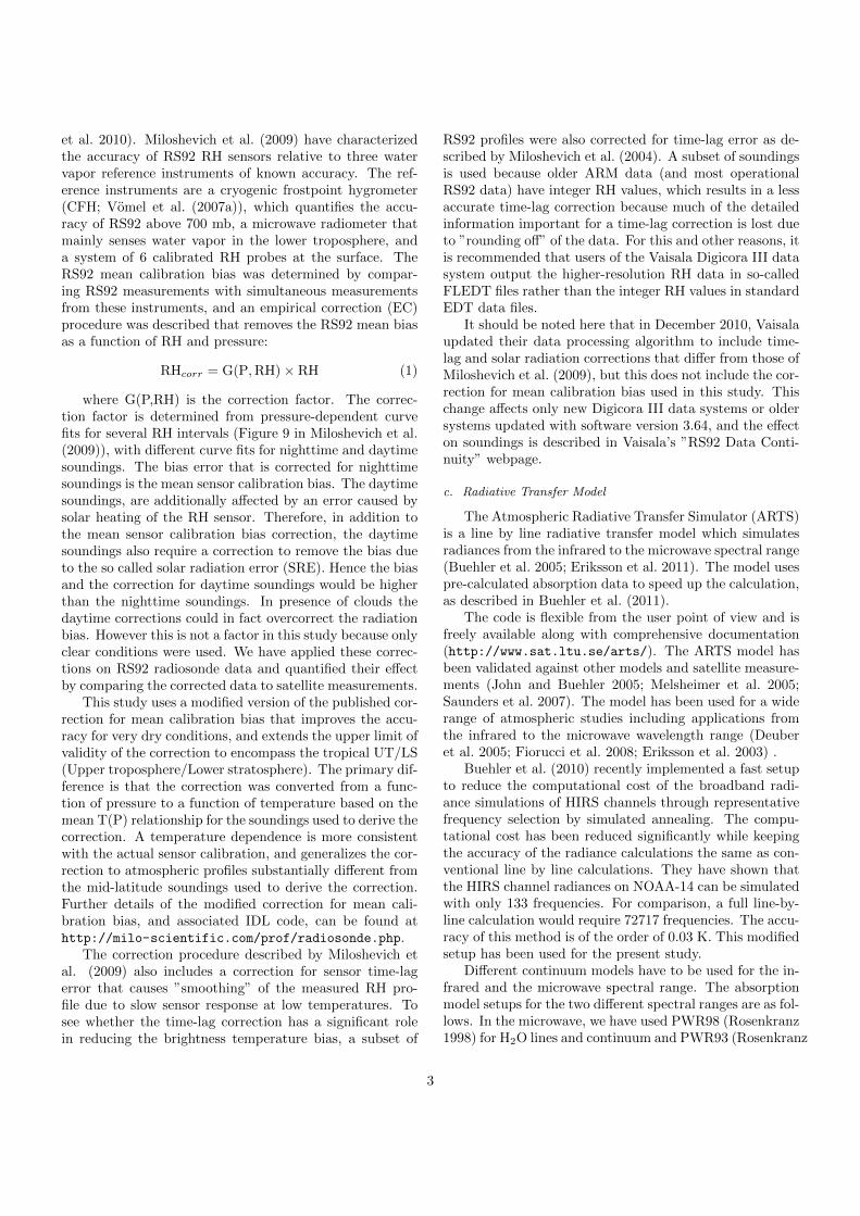
et al. 2010). Miloshevich et al. (2009) have characterizedthe accuracy of RS92 RH sensors relative to three watervapor reference instruments of known accuracy. The ref-erence instruments are a cryogenic frostpoint hygrometer(CFH; Vomel et al. (2007a)), which quantifies the accu-racy of RS92 above 700 mb, a microwave radiometer thatmainly senses water vapor in the lower troposphere, anda system of 6 calibrated RH probes at the surface. TheRS92 mean calibration bias was determined by compar-ing RS92 measurements with simultaneous measurementsfrom these instruments, and an empirical correction (EC)procedure was described that removes the RS92 mean biasas a function of RH and pressure:

RHcorr = G(P,RH)× RH (1)

where G(P,RH) is the correction factor. The correc-tion factor is determined from pressure-dependent curvefits for several RH intervals (Figure 9 in Miloshevich et al.(2009)), with different curve fits for nighttime and daytimesoundings. The bias error that is corrected for nighttimesoundings is the mean sensor calibration bias. The daytimesoundings, are additionally affected by an error caused bysolar heating of the RH sensor. Therefore, in addition tothe mean sensor calibration bias correction, the daytimesoundings also require a correction to remove the bias dueto the so called solar radiation error (SRE). Hence the biasand the correction for daytime soundings would be higherthan the nighttime soundings. In presence of clouds thedaytime corrections could in fact overcorrect the radiationbias. However this is not a factor in this study because onlyclear conditions were used. We have applied these correc-tions on RS92 radiosonde data and quantified their effectby comparing the corrected data to satellite measurements.

This study uses a modified version of the published cor-rection for mean calibration bias that improves the accu-racy for very dry conditions, and extends the upper limit ofvalidity of the correction to encompass the tropical UT/LS(Upper troposphere/Lower stratosphere). The primary dif-ference is that the correction was converted from a func-tion of pressure to a function of temperature based on themean T(P) relationship for the soundings used to derive thecorrection. A temperature dependence is more consistentwith the actual sensor calibration, and generalizes the cor-rection to atmospheric profiles substantially different fromthe mid-latitude soundings used to derive the correction.Further details of the modified correction for mean cali-bration bias, and associated IDL code, can be found athttp://milo-scientific.com/prof/radiosonde.php.

The correction procedure described by Miloshevich etal. (2009) also includes a correction for sensor time-lagerror that causes ”smoothing” of the measured RH pro-file due to slow sensor response at low temperatures. Tosee whether the time-lag correction has a significant rolein reducing the brightness temperature bias, a subset of

RS92 profiles were also corrected for time-lag error as de-scribed by Miloshevich et al. (2004). A subset of soundingsis used because older ARM data (and most operationalRS92 data) have integer RH values, which results in a lessaccurate time-lag correction because much of the detailedinformation important for a time-lag correction is lost dueto ”rounding off” of the data. For this and other reasons, itis recommended that users of the Vaisala Digicora III datasystem output the higher-resolution RH data in so-calledFLEDT files rather than the integer RH values in standardEDT data files.

It should be noted here that in December 2010, Vaisalaupdated their data processing algorithm to include time-lag and solar radiation corrections that differ from those ofMiloshevich et al. (2009), but this does not include the cor-rection for mean calibration bias used in this study. Thischange affects only new Digicora III data systems or oldersystems updated with software version 3.64, and the effecton soundings is described in Vaisala’s ”RS92 Data Conti-nuity” webpage.

c. Radiative Transfer Model

The Atmospheric Radiative Transfer Simulator (ARTS)is a line by line radiative transfer model which simulatesradiances from the infrared to the microwave spectral range(Buehler et al. 2005; Eriksson et al. 2011). The model usespre-calculated absorption data to speed up the calculation,as described in Buehler et al. (2011).

The code is flexible from the user point of view and isfreely available along with comprehensive documentation(http://www.sat.ltu.se/arts/). The ARTS model hasbeen validated against other models and satellite measure-ments (John and Buehler 2005; Melsheimer et al. 2005;Saunders et al. 2007). The model has been used for a widerange of atmospheric studies including applications fromthe infrared to the microwave wavelength range (Deuberet al. 2005; Fiorucci et al. 2008; Eriksson et al. 2003) .

Buehler et al. (2010) recently implemented a fast setupto reduce the computational cost of the broadband radi-ance simulations of HIRS channels through representativefrequency selection by simulated annealing. The compu-tational cost has been reduced significantly while keepingthe accuracy of the radiance calculations the same as con-ventional line by line calculations. They have shown thatthe HIRS channel radiances on NOAA-14 can be simulatedwith only 133 frequencies. For comparison, a full line-by-line calculation would require 72717 frequencies. The accu-racy of this method is of the order of 0.03 K. This modifiedsetup has been used for the present study.

Different continuum models have to be used for the in-frared and the microwave spectral range. The absorptionmodel setups for the two different spectral ranges are as fol-lows. In the microwave, we have used PWR98 (Rosenkranz1998) for H2O lines and continuum and PWR93 (Rosenkranz

3

1993) for N2 and O2 lines and their respective continuum.Furthermore, line data of O3 was taken from HITRAN 2004(Rothman et al. 2003). In the infrared, line data were takenfrom HITRAN 2004 while the continua of H2O, CH4, N2,O2 and CO2 were taken from MT CKD 1.0 (Mlawer et al.2003). A model inter-comparison study between ARTS andthe Line-Line Radiative Transfer model (LBLRTM), an es-tablished reference model for the infrared spectral rangewas carried out for HIRS 12 on NOAA satellites 14, 15 16and 17. The model comparison approach is described inAppendix A. The two radiative transfer (RT) models werefound to agree within a brightness temperature differenceof 0.22 K. ARTS includes various algorithms to simulatethe influence of clouds (Davis et al. 2005; Emde et al. 2004).However, for the present study only clear sky simulationswere performed.

d. Collocations and Cloud Detection Approach

The collocations between NOAA-17 measurements andARM radiosondes are based on spatial and temporal con-straints. The spatial constraint is implemented by a targetarea of radius 50 km around the radiosonde location asin Buehler et al. (2004). This approximately takes intoaccount the drift of the radiosonde as it ascends throughthe atmosphere. The number of collocated pixels in a tar-get area varies from 2–8 for HIRS 12 and from 10–30 forAMSU 18 respectively. The time constraint imposed onthe collocated dataset is ±2 hours. This should accommo-date the time taken for the radiosonde to reach the satellitemeasuring altitude peak (300 hPa) which is approximately25 minutes. Hence, the radiosonde time in the collocateddataset is the sum of the radiosonde launch time and 25minutes. Radiances are simulated from radiosonde profilesusing ARTS to match with the satellite viewing geometry.

A meaningful comparison between satellite measure-ments and clear sky RT model simulations is possible onlyif the measurements are free of cloud contamination. There-fore we use the cloud detection tests developed by McMillinand Dean (1982) to filter out contaminated HIRS pixelsfrom our analysis. Details of this procedure are as follows.

Each pixel from satellite measurements is subjected tothe following cloud detection tests. The first two tests arebased on the long-wave window channel (11 µm ) bright-ness temperature and is applicable to all the measurements.

i. A pixel is classified as cloudy if its window channelbrightness temperature is too cold ( < 210 K).

ii. A pixel is classified as cloudy, if the long-wave windowchannel brightness temperature is 4 K cooler thanthat of the warmest pixel from the target area.

iii. If any one of the followings conditions fail for nighttime measurements, then the pixel is classified ascloudy.

−4.0 K ≤ TB(18)-TB(8) ≤ 2.0 K

−4.0 K ≤ TB(19)-TB(18) ≤ 2.0 K

iv. During the day a pixel is clear if

|TB(18)− TB(8)| < 10 K

where TB(i) is the brightness temperature for a givenHIRS channel i. If there is more than one clear pixel in thetarget area, the average over all the clear pixels are usedotherwise it is classified as cloudy. This very stringent clearscene requirement condition satisfies 25 to 100 % of thetarget area for HIRS depending on the cloud cover. Weassume that the AMSU 18 pixels coincident to the clearHIRS 12 pixels are not cloud contaminated. This couldeven result in the removal of the AMSU 18 pixel which areunaffected by clouds due to the much higher sensitivity ofHIRS measurements to thin clouds.

e. Relation between UTH and Brightness temperature

The relationship between UTH and brightness temper-ature Tb is given by,

ln(UTH) = a + b× Tb (2)

where a and b can be determined by linear regression. Thederivative yields

∆UTH

UTH= b×∆T (3)

In other words, absolute changes in brightness temper-ature map to relative changes in UTH. To ensure completeconsistency here, we have re-determined the parametersbHIRS 12 and bAMSU 18 using linear regression on the simu-lated measurements for the Chevallier et al. (2006) data set.The values obtained for bHIRS 12 and bAMSU 18 are 0.110and 0.070 for the nadir viewing direction. For the extremeoff-nadir viewing direction the bHIRS 12 and bAMSU 18 val-ues are 0.118 and 0.076. These values are in good agree-ment with Soden and Bretherton (1993) and Buehler andJohn (2005). The regression coefficients a and b for dif-ferent viewing angles of HIRS 12 are summarised in Table1.

f. Ozone Impact on AMSU 18 Radiances

The impact of ozone lines on AMSU-B radiances wasinvestigated by John and Buehler (2004). They found thatthe ozone impact is largest for AMSU 18. This can re-duce its brightness temperature, with a reduction that canreach a maximum of 0.5 K. It was also reported that zonal,monthly mean climatological values of ozone profiles aresufficient to account for the ozone impact on AMSU 18 ra-diances. With the above work as a base, temperature andhumidity profiles from ARM radiosondes were taken up to100 hPa and the rest of the pressure levels up to 0.2 hPa

4

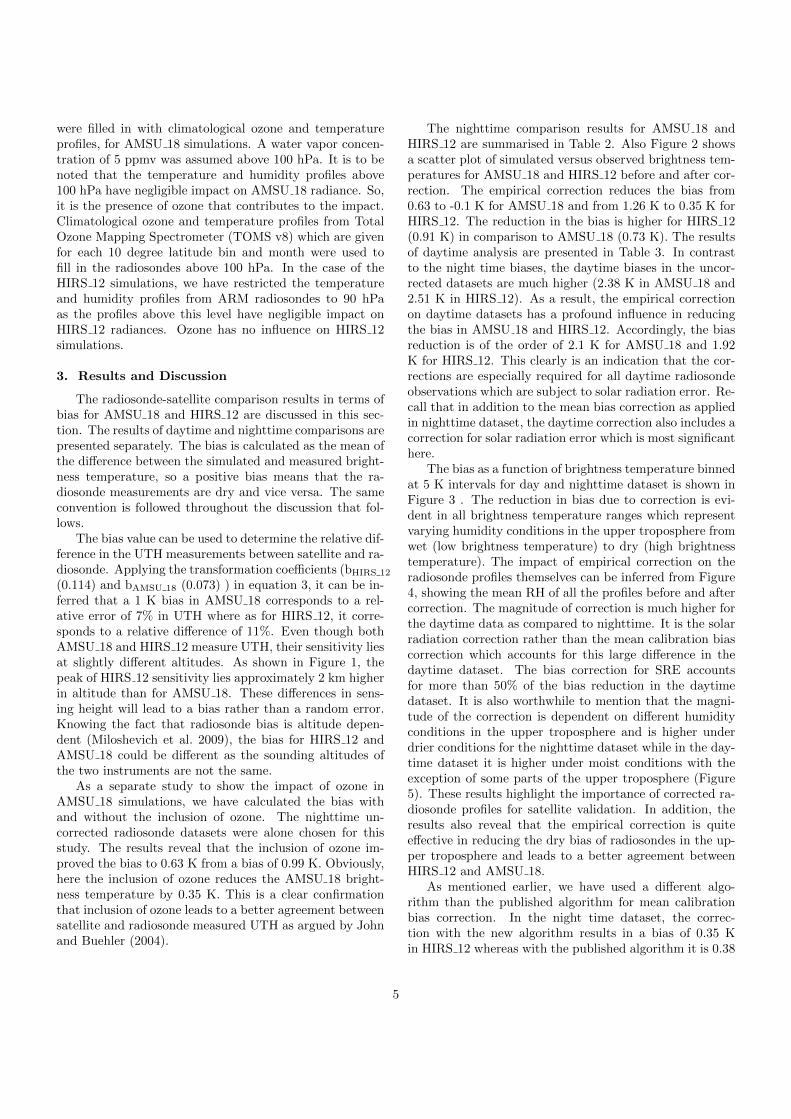
were filled in with climatological ozone and temperatureprofiles, for AMSU 18 simulations. A water vapor concen-tration of 5 ppmv was assumed above 100 hPa. It is to benoted that the temperature and humidity profiles above100 hPa have negligible impact on AMSU 18 radiance. So,it is the presence of ozone that contributes to the impact.Climatological ozone and temperature profiles from TotalOzone Mapping Spectrometer (TOMS v8) which are givenfor each 10 degree latitude bin and month were used tofill in the radiosondes above 100 hPa. In the case of theHIRS 12 simulations, we have restricted the temperatureand humidity profiles from ARM radiosondes to 90 hPaas the profiles above this level have negligible impact onHIRS 12 radiances. Ozone has no influence on HIRS 12simulations.

3. Results and Discussion

The radiosonde-satellite comparison results in terms ofbias for AMSU 18 and HIRS 12 are discussed in this sec-tion. The results of daytime and nighttime comparisons arepresented separately. The bias is calculated as the mean ofthe difference between the simulated and measured bright-ness temperature, so a positive bias means that the ra-diosonde measurements are dry and vice versa. The sameconvention is followed throughout the discussion that fol-lows.

The bias value can be used to determine the relative dif-ference in the UTH measurements between satellite and ra-diosonde. Applying the transformation coefficients (bHIRS 12

(0.114) and bAMSU 18 (0.073) ) in equation 3, it can be in-ferred that a 1 K bias in AMSU 18 corresponds to a rel-ative error of 7% in UTH where as for HIRS 12, it corre-sponds to a relative difference of 11%. Even though bothAMSU 18 and HIRS 12 measure UTH, their sensitivity liesat slightly different altitudes. As shown in Figure 1, thepeak of HIRS 12 sensitivity lies approximately 2 km higherin altitude than for AMSU 18. These differences in sens-ing height will lead to a bias rather than a random error.Knowing the fact that radiosonde bias is altitude depen-dent (Miloshevich et al. 2009), the bias for HIRS 12 andAMSU 18 could be different as the sounding altitudes ofthe two instruments are not the same.

As a separate study to show the impact of ozone inAMSU 18 simulations, we have calculated the bias withand without the inclusion of ozone. The nighttime un-corrected radiosonde datasets were alone chosen for thisstudy. The results reveal that the inclusion of ozone im-proved the bias to 0.63 K from a bias of 0.99 K. Obviously,here the inclusion of ozone reduces the AMSU 18 bright-ness temperature by 0.35 K. This is a clear confirmationthat inclusion of ozone leads to a better agreement betweensatellite and radiosonde measured UTH as argued by Johnand Buehler (2004).

The nighttime comparison results for AMSU 18 andHIRS 12 are summarised in Table 2. Also Figure 2 showsa scatter plot of simulated versus observed brightness tem-peratures for AMSU 18 and HIRS 12 before and after cor-rection. The empirical correction reduces the bias from0.63 to -0.1 K for AMSU 18 and from 1.26 K to 0.35 K forHIRS 12. The reduction in the bias is higher for HIRS 12(0.91 K) in comparison to AMSU 18 (0.73 K). The resultsof daytime analysis are presented in Table 3. In contrastto the night time biases, the daytime biases in the uncor-rected datasets are much higher (2.38 K in AMSU 18 and2.51 K in HIRS 12). As a result, the empirical correctionon daytime datasets has a profound influence in reducingthe bias in AMSU 18 and HIRS 12. Accordingly, the biasreduction is of the order of 2.1 K for AMSU 18 and 1.92K for HIRS 12. This clearly is an indication that the cor-rections are especially required for all daytime radiosondeobservations which are subject to solar radiation error. Re-call that in addition to the mean bias correction as appliedin nighttime dataset, the daytime correction also includes acorrection for solar radiation error which is most significanthere.

The bias as a function of brightness temperature binnedat 5 K intervals for day and nighttime dataset is shown inFigure 3 . The reduction in bias due to correction is evi-dent in all brightness temperature ranges which representvarying humidity conditions in the upper troposphere fromwet (low brightness temperature) to dry (high brightnesstemperature). The impact of empirical correction on theradiosonde profiles themselves can be inferred from Figure4, showing the mean RH of all the profiles before and aftercorrection. The magnitude of correction is much higher forthe daytime data as compared to nighttime. It is the solarradiation correction rather than the mean calibration biascorrection which accounts for this large difference in thedaytime dataset. The bias correction for SRE accountsfor more than 50% of the bias reduction in the daytimedataset. It is also worthwhile to mention that the magni-tude of the correction is dependent on different humidityconditions in the upper troposphere and is higher underdrier conditions for the nighttime dataset while in the day-time dataset it is higher under moist conditions with theexception of some parts of the upper troposphere (Figure5). These results highlight the importance of corrected ra-diosonde profiles for satellite validation. In addition, theresults also reveal that the empirical correction is quiteeffective in reducing the dry bias of radiosondes in the up-per troposphere and leads to a better agreement betweenHIRS 12 and AMSU 18.

As mentioned earlier, we have used a different algo-rithm than the published algorithm for mean calibrationbias correction. In the night time dataset, the correc-tion with the new algorithm results in a bias of 0.35 Kin HIRS 12 whereas with the published algorithm it is 0.38

5

K, but for AMSU 18 these values are -0.07 K and -0.10K respectively. For the daytime dataset, correction withthe new algorithm yields a bias of 1.71 K in HIRS 12 anda bias of 1.75 K with the published algorithm, while inAMSU 18 these values are 1.76 K and 1.78 K respectively.Though these differences are small the use of the new al-gorithm is recommended for mean calibration correctionsince the temperature dependence is more consistent withactual sensor calibration than the pressure dependence asused in the published algorithm.

The impact of the time lag (TL) correction is shownin Table 4. This result reveals that the TL correction hasa negligible impact in reducing the bias in AMSU 18 andHIRS 12 because the bias reduction is of the order of only0.03 K. Since TL correction needs profiles of higher res-olution, it is applied here only to a subset of RS92 pro-files. A noteworthy observation is that the bias reductionin AMSU 18 and HIRS 12 due to empirical correction onthis subset is the same as that for all the RS92 profiles (notshown).

Though the agreement between HIRS 12 and AMSU 18has been improved due to correction, a small discrepancyof the order of 0.45 K for nighttime and 0.31 K for day-time data still remains. One of the major reasons for thediscrepancy can be attributed to the uncertainty in thecorrected RS92 measurements. Miloshevich et al. (2009)have shown that the bias uncertainty is ±(4% + 0.5 %RH),which implies 4% of the measured value plus a 0.5 %RHoffset component that is increasingly important for drierconditions. For example, the relative uncertainty in thecorrected RS92 data is ±5% for conditions of 50 %RH,±6.5% at 20 %RH, ±9% at 10 %RH, and ±20% at 3 %RH.Therefore, there could be a larger uncertainty in the cor-rection occurring at the HIRS 12 sensing altitude than atthe AMSU 18 sensing altitude as it senses a drier atmo-sphere. A part of the difference could also be attributed toerror in the radiative transfer modeling. However, basedon the comparison to LBLRTM described in Appendix A,we expect this error to be smaller than 0.3 K. Systematicerror in the satellite measurements which is of the orderof 0.5 K in AMSU 18 and HIRS 12 on NOAA-17 couldalso play a role (Shi and Bates 2011; John et al. submitted2011). It is difficult to attribute the remaining discrep-ancy between AMSU 18 and HIRS 12 to any single causeas it a very small bias. Therefore, it is only fair to saythat the radiosonde, radiative transfer modelling and sys-tematic error in AMSU/HIRS measurements are equallyplausible contributors to the bias.

Coming back to the subject of radiosonde correction,one can state that in addition to significantly reducing thebias between satellite and radiosonde measurements, em-pirical correction also brings forth a better agreement be-tween AMSU 18 and HIRS 12. The discrepancy in theapparent radiosonde bias between HIRS 12 and AMSU 18

before correction in nighttime dataset was around 10% andit was lowered to approximately 5% after correction. Sim-ilarly, the discrepancy in the uncorrected daytime datasetwas 12% which reduces to 4.7% after correction. These re-sults show that the radiosonde correction is very importantin bringing about a better agreement between satellite andradiosonde measurements of UTH.

There have been a number of earlier correction meth-ods for improving the accuracy of RS80 radiosonde sensors(Turner et al. 2003; Miloshevich et al. 2001). However, So-den et al. (2004) showed that these correction proceduresoffer only a small improvement in the upper troposphere,though they are effective in the lower troposphere. In con-trast to this, our work for the RS92 sensors and Miloshe-vich et al. (2009) correction method, shows a significantimprovement, particularly, in the upper troposphere. Thepresent study therefore may open up the possibility of ap-plying a similar correction approach to other radiosondesensors.

4. Summary and Conclusions

The present study evaluates the importance of radiosondecorrection in improving the agreement between satelliteand radiosonde measured UTH. The satellite measurementsfrom infrared (HIRS 12) and microwave (AMSU 18) in-struments were used for this purpose. The satellite mea-surements were collocated with ARM radiosonde profiles.The satellite-radiosonde comparison was performed by sim-ulating the radiances from collocated radiosonde profilesusing the radiative transfer model ARTS. The compar-isons were performed only for clear sky conditions. Theempirical correction procedure applied to RS92 radiosondesensors was found to have a significant impact in reducingthe bias in AMSU 18 and HIRS 12. The nighttime bias inAMSU 18 (from 0.63 K to -0.10 K) was reduced by 0.73 Kand by 0.91 K in HIRS 12 (from 1.26 K to 0.35 K). Duringdaytime, the decrease in bias is significantly higher with areduction of 2.1 K (from 2.38 K to 0.28 K) in AMSU 18and 1.92 K (from 2.51 K to 0.59 K) in HIRS 12. This is onaccount of the bias removal associated with the solar radi-ation error. The correction also improved the consistencybetween AMSU 18 and HIRS 12 and reduced the differencebetween them by 5% in nighttime and by 7% in daytimedatasets.

Besides showing the importance of radiosonde correc-tion for satellite validation, this study also cautions againstthe use of uncorrected radiosonde profiles for various watervapour related studies in the upper troposphere. The needfor such corrections is especially due to the imperfect char-acterization and calibration of the sensor output by themanufacturer. The occurrence of a similar or worse typeof imperfection as addressed here for Vaisala radiosondescannot be ruled out for many other operational radioson-

6

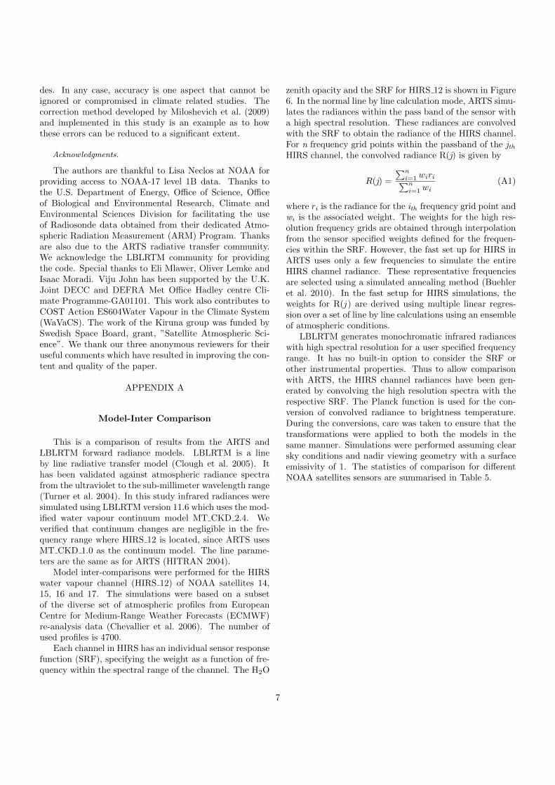
des. In any case, accuracy is one aspect that cannot beignored or compromised in climate related studies. Thecorrection method developed by Miloshevich et al. (2009)and implemented in this study is an example as to howthese errors can be reduced to a significant extent.

Acknowledgments.

The authors are thankful to Lisa Neclos at NOAA forproviding access to NOAA-17 level 1B data. Thanks tothe U.S. Department of Energy, Office of Science, Officeof Biological and Environmental Research, Climate andEnvironmental Sciences Division for facilitating the useof Radiosonde data obtained from their dedicated Atmo-spheric Radiation Measurement (ARM) Program. Thanksare also due to the ARTS radiative transfer community.We acknowledge the LBLRTM community for providingthe code. Special thanks to Eli Mlawer, Oliver Lemke andIsaac Moradi. Viju John has been supported by the U.K.Joint DECC and DEFRA Met Office Hadley centre Cli-mate Programme-GA01101. This work also contributes toCOST Action ES604Water Vapour in the Climate System(WaVaCS). The work of the Kiruna group was funded bySwedish Space Board, grant, ”Satellite Atmospheric Sci-ence”. We thank our three anonymous reviewers for theiruseful comments which have resulted in improving the con-tent and quality of the paper.

APPENDIX A

Model-Inter Comparison

This is a comparison of results from the ARTS andLBLRTM forward radiance models. LBLRTM is a lineby line radiative transfer model (Clough et al. 2005). Ithas been validated against atmospheric radiance spectrafrom the ultraviolet to the sub-millimeter wavelength range(Turner et al. 2004). In this study infrared radiances weresimulated using LBLRTM version 11.6 which uses the mod-ified water vapour continuum model MT CKD 2.4. Weverified that continuum changes are negligible in the fre-quency range where HIRS 12 is located, since ARTS usesMT CKD 1.0 as the continuum model. The line parame-ters are the same as for ARTS (HITRAN 2004).

Model inter-comparisons were performed for the HIRSwater vapour channel (HIRS 12) of NOAA satellites 14,15, 16 and 17. The simulations were based on a subsetof the diverse set of atmospheric profiles from EuropeanCentre for Medium-Range Weather Forecasts (ECMWF)re-analysis data (Chevallier et al. 2006). The number ofused profiles is 4700.

Each channel in HIRS has an individual sensor responsefunction (SRF), specifying the weight as a function of fre-quency within the spectral range of the channel. The H2O

zenith opacity and the SRF for HIRS 12 is shown in Figure6. In the normal line by line calculation mode, ARTS simu-lates the radiances within the pass band of the sensor witha high spectral resolution. These radiances are convolvedwith the SRF to obtain the radiance of the HIRS channel.For n frequency grid points within the passband of the jthHIRS channel, the convolved radiance R(j) is given by

R(j) =

∑ni=1 wiri∑ni=1 wi

(A1)

where ri is the radiance for the ith frequency grid point andwi is the associated weight. The weights for the high res-olution frequency grids are obtained through interpolationfrom the sensor specified weights defined for the frequen-cies within the SRF. However, the fast set up for HIRS inARTS uses only a few frequencies to simulate the entireHIRS channel radiance. These representative frequenciesare selected using a simulated annealing method (Buehleret al. 2010). In the fast setup for HIRS simulations, theweights for R(j ) are derived using multiple linear regres-sion over a set of line by line calculations using an ensembleof atmospheric conditions.

LBLRTM generates monochromatic infrared radianceswith high spectral resolution for a user specified frequencyrange. It has no built-in option to consider the SRF orother instrumental properties. Thus to allow comparisonwith ARTS, the HIRS channel radiances have been gen-erated by convolving the high resolution spectra with therespective SRF. The Planck function is used for the con-version of convolved radiance to brightness temperature.During the conversions, care was taken to ensure that thetransformations were applied to both the models in thesame manner. Simulations were performed assuming clearsky conditions and nadir viewing geometry with a surfaceemissivity of 1. The statistics of comparison for differentNOAA satellites sensors are summarised in Table 5.

7

−0.05 0 0.05 0.1 0.15 0.2

101

102

103

Jacobian [K/1]

Pre

ssur

e [h

Pa]

AMSU_18HIRS_12

Fig. 1. Jacobian of AMSU 18 and HIRS 12 UTH channels for the standard tropical atmosphere (Garand et al. 2001)with a nadir viewing geometry. Jacobian values are divided by their sum.

8

Table 1. The regression coefficients a and b used to derive UTH from HIRS 12 for its different viewing angles. TheUTH is defined with respect to liquid water. The angle θ is in degrees, a is dimensionless, and b is in K−1.

θ a b0.900 29.554 -0.1102.700 29.556 -0.1104.500 29.560 -0.1106.300 29.566 -0.1108.100 29.574 -0.1109.900 29.584 -0.11011.700 29.596 -0.11013.500 29.610 -0.11015.300 29.626 -0.11117.100 29.645 -0.11118.900 29.667 -0.11120.700 29.691 -0.11122.500 29.718 -0.11124.300 29.748 -0.11126.100 29.781 -0.11227.900 29.818 -0.11229.700 29.859 -0.11231.500 29.904 -0.11233.300 29.955 -0.11335.100 30.011 -0.11336.900 30.073 -0.11338.700 30.143 -0.11440.500 30.222 -0.11442.300 30.311 -0.11544.100 30.412 -0.11645.900 30.529 -0.11647.700 30.666 -0.11749.500 30.828 -0.118

9

220 240 260 280220

230

240

250

260

270

280

Satellite AMSU_18 [K]

Sim

ulat

ed A

MS

U_1

8 [K

]

Mean Bias = 0.63 KSlope = 1.029cc= 0.97

220 240 260 280220

230

240

250

260

270

280

Satellite HIRS_12 [K]

Sim

ulat

ed H

IRS

_12

[K]


220 240 260 280220

230

240

250

260

270

280

Satellite AMSU_18 [K]

Sim

ulat

ed A

MS

U_1

8 [K

]

Mean Bias = −0.10 KSlope = 1.045cc= 0.97

220 240 260 280220

230

240

250

260

270

280

Satellite HIRS_12 [K]S

imul

ated

HIR

S_1

2 [K

]


Fig. 2. Scatter plots of simulated versus observed brightness temperature for AMSU 18 and HIRS 12 before (upperpanels) and after empirical correction (lower panels, corrected RS92) for the nighttime data. The black and red lines arediagonal and regression lines respectively. The number of datapoints is 624 for each plot.

230 240 250 260 270−1

−0.5

0

0.5

1

1.5

AMSU_18 [K]

Bia

s [K

]

CorrectedOriginal

220 230 240 250 260−0.5

0

0.5

1

1.5

2

2.5

HIRS_12 [K]

Bia

s [K

]

230 240 250 260 270−1

0

1

2

3

AMSU_18 [K]

Bia

s [K

]

220 230 240 250 2600

0.5

1

1.5

2

2.5

3

HIRS_12 [K]

Bia

s [K

]

Fig. 3. Bias as a function of brightness temperature binned at 5 K intervals before (red) and after (blue) Empiricalcorrection for AMSU 18 (left) and HIRS 12 (right). The vertical bars represent the standard error. Upper panels are fornighttime data, lower panels are for daytime data.

10

0 20 40 60

102

103

Relative Humidity (%RH)

Pre

ssur

e [h

Pa]

OriginalCorrected

−20 0 20 40

102

103

Difference (%)

Pre

ssur

e [h

Pa]

0 20 40 60

102

103

Relative Humidity (%RH)

Pre

ssur

e [h

Pa]

−50 0 50 100

102

103

Difference (%)

Pre

ssur

e [h

Pa]

Fig. 4. Left: The mean RH of RS92 radiosonde sensors before (black) and after Empirical correction. Right: The thickline represents mean of the percentage difference between the corrected and the original profiles. The horizontal barsrepresent the standard deviation. For the figure RH profiles from ARM radiosondes before and after the correctionswere interpolated to specific pressure levels (53) ranging from 980 to 100 hPa. The Percentage difference is defined as(

corrected−originaloriginal

)× 100%. Upper panels are for nighttime data, lower panels are for daytime data.

−10 0 10 20 30

102

103

Difference (%)

Pre

ssur

e [h

Pa]

DryMoistModerate

0 20 40 60

102

103

Difference (%)

Pre

ssur

e [h

Pa]

Fig. 5. The percentage difference between the corrected and original profiles classified in terms of different humidityconditions in the upper troposphere (dry, moist and moderate). Classification is based on the percentiles of the observedbrightness temperature in HIRS 12 such that values ≥ 75 percentile are considerd as dry, ≤ 25 percentile moist and valuesranging between these as moderate. Left plot is for nighttime data and the right plot is for daytime data.

11

1480 1490 1500 1510 1520 1530 1540 1550 1560 1570 1580

101

102

103

104

105

Opa

city

Wavenumber [cm −1]

1480 1490 1500 1510 1520 1530 1540 1550 1560 1570 15800

0.04

0.08

0.12

0.16

0.2

Cha

nnel

Res

pons

e

Fig. 6. The H2O zenith opacity spectrum (blue) and the SRF for HIRS 12 (black) on NOAA-17.

12

Table 2. Statistics comparing satellite radiance and simulated radiance in brightness temperature units for the nighttimedatset. The bias is defined as the mean of simulated minus measured data. SD refers to the standard deviation. Thenumber of profiles used is 624. Suffix bc and ac refers to before and after empirical correction.

Channel Bias (K) Bias in UTH (%) SD (K) SD UTH (%)AMSU 18bc 0.63 -4.5 1.66 11.62AMSU 18ac -0.10 0.7 1.68 11.76HIRS 12bc 1.26 -14.3 1.40 16HIRS 12ac 0.35 -3.9 1.42 16.18

Table 3. Statistics comparing satellite radiance and simulated radiance in brightness temperature units for the daytimedataset. The bias is defined as the mean of simulated minus measured data. SD refers to the standard deviation. Thenumber of profiles used is 419. Suffix bc and ac refers to before and after empirical correction.

Channel Bias (K) Bias in UTH (%) SD (K) SD UTH (%)AMSU 18bc 2.38 -16.6 1.31 9.17AMSU 18ac 0.28 -1.96 1.39 9.73HIRS 12bc 2.51 -28.61 1.19 13.57HIRS 12ac 0.59 - 6.73 1.27 14.48

Table 4. Statistics comparing satellite radiance and simulated radiance in brightness temperature units for RS92 sensors.The bias is defined as the mean of simulated minus measured data. SD refers to the standard deviation. The number ofprofiles used is 85. Suffix btl and atl refers to before and after time lag correction.

Channel Bias (K) Bias in UTH (%) SD (K) SD UTH (%)AMSU 18btl 0.14 -0.9 1.52 10.64AMSU 18atl 0.17 -1.2 1.51 10.57HIRS 12btl 0.94 -10.7 1.21 13.80HIRS 12atl 0.91 -10.4 1.19 13.56

Table 5. Statistics comparing ARTS and LBLRTM simulations. The bias is defined as the mean of the difference ARTSminus LBLRTM. SD refers to the standard deviation.

Satellite Channel Bias (K) SD (K)NOAA-14 HIRS 12 -0.07 0.15NOAA-15 HIRS 12 -0.21 0.23NOAA-16 HIRS 12 -0.17 0.22NOAA-17 HIRS 12 -0.21 0.22

13

REFERENCES

Buehler, S. A., P. Eriksson, T. Kuhn, A. von Engeln,and C. Verdes, 2005: ARTS, the atmospheric radiativetransfer simulator. J. Quant. Spectrosc. Radiat. Trans-fer, 91 (1), 65–93, doi:10.1016/j.jqsrt.2004.05.051.

Buehler, S. A., P. Eriksson, and O. Lemke, 2011: Absorp-tion lookup tables in the radiative transfer model arts.J. Quant. Spectrosc. Radiat. Transfer, 112 (10), 1559–1567, doi:10.1016/j.jqsrt.2011.03.008.

Buehler, S. A. and V. O. John, 2005: A simple methodto relate microwave radiances to upper tropospheric hu-midity. J. Geophys. Res., 110, D02110, doi:10.1029/2004JD005111.

Buehler, S. A., V. O. John, A. Kottayil, M. Milz, andP. Eriksson, 2010: Efficient radiative transfer simula-tions for a broadband infrared radiometer — combin-ing a weighted mean of representative frequencies ap-proach with frequency selection by simulated annealing.J. Quant. Spectrosc. Radiat. Transfer, 111 (4), 602–615,doi:10.1016/j.jqsrt.2009.10.018.

Buehler, S. A., M. Kuvatov, V. O. John, U. Leiterer, andH. Dier, 2004: Comparison of microwave satellite humid-ity data and radiosonde profiles: A case study. J. Geo-phys. Res., 109, D13103, doi:10.1029/2004JD004605.

Buehler, S. A., M. Kuvatov, V. O. John, M. Milz, B. J.Soden, D. L. Jackson, and J. Notholt, 2008: An uppertropospheric humidity data set from operational satellitemicrowave data. J. Geophys. Res., 113, D14110, doi:10.1029/2007JD009314.

Chevallier, F., S. Di Michele, and A. P. McNally, 2006: Di-verse profile datasets from the ECMWF 91-level short-range forecasts. Tech. rep., NWP SAF Satellite Appli-cation Facility for Numerical Weather Prediction. Doc-ument No. NWPSAF-EC-TR-010, Version 1.0.

Clough, S. A., M. W. Shephard, E. J. Mlawer, J. S. De-lamere, M. J. Iacono, K. Cady-Pereira, S. Boukabara,and P. D. Brown, 2005: Atmospheric radiative trans-fer modeling: a summary of the AER codes. Journal ofQuantitative Spectroscopy and Radiative Transfer, 91,233–244, doi:10.1016/j.jqsrt.2004.05.058.

Davis, C., C. Emde, and R. Harwood, 2005: A 3D po-larized reversed monte carlo radiative transfer model formm and sub-mm passive remote sensing in cloudy atmo-spheres. IEEE T. Geosci. Remote, 43 (5), 1096–1101,doi:10.1109/TGRS.2004.837505.

Deuber, B., J. Morland, L. Martin, and N. Kampfer, 2005:Deriving the tropospheric integrated water vapor fromtipping curve-derived opacity near 22 GHz. Radio Sci.,40, RS5011, doi:10.1029/2007RG000233.

Elliott, W. P. and D. J. Gaffen, 1991: On the Utility ofRadiosonde Humidity Archives for Climate Studies. Bul-letin of the American Meteorological Society, 72, 1507–1520, doi:10.1175/1520-0477(1991)072〈1507:OTUORH〉2.0.CO;2.

Emde, C., S. Buehler, C. Davis, P. Eriksson, T. Sreerekha,and C. Teichmann, 2004: A polarized discrete or-dinate scattering model for simulations of limb andnadir long-wave measurements in 1-D/3-D spher-ical atmospheres. JOURNAL OF GEOPHYSICALRESEARCH-ATMOSPHERES, 109 (D24), doi:{10.1029/2004JD005140}.

Eriksson, P., S. A. Buehler, C. P. Davis, C. Emde, andO. Lemke, 2011: ARTS, the atmospheric radiative trans-fer simulator, version 2. J. Quant. Spectrosc. Radiat.Transfer, 112 (10), 1551–1558, doi:10.1016/j.jqsrt.2011.03.001.

Eriksson, P., C. Jimenez, D. Murtagh, G. Elgered,T. Kuhn, and S. Buehler, 2003: Measurement of tro-pospheric/stratospheric transmission at 10–35 GHz forH2O retrieval in low earth orbiting satellite links. RadioSci., 38 (4), 8069, doi:10.1029/2002RS002638.

Fiorucci, I., et al., 2008: Measurements of low amountsof precipitable water vapor by millimeter wave spec-troscopy: An intercomparison with radiosonde, ramanlidar, and fourier transform infrared data. J. Geophys.Res., 113, D14314, doi:10.1029/2008JD009831.

Garand, L. et al., 2001: Radiance and jacobian intercom-parison of radiative transfer models applied to HIRS andAMSU channels. J. Geophys. Res., 106 (D20), 24,017–24,031.

Held, I. M. and B. J. Soden, 2000: Water vapor feedbackand global warming. Annu. Rev. Energy Environ., 25,441–475.

John, V. O. and S. A. Buehler, 2004: The impact of ozonelines on AMSU-B radiances. Geophys. Res. Lett., 31,L21108, doi:10.1029/2004GL021214.

John, V. O. and S. A. Buehler, 2005: Comparison of mi-crowave satellite humidity data and radiosonde profiles:A survey of European stations. Atmos. Chem. Phys., 5,1843–1853, doi:10.5194/acp-5-1843-2005, sRef-ID:1680-7324/acp/2005-5-1843.

John, V. O., G. Holl, S. A. Buehler, B. Candy, R. W. Saun-ders, and D. E. Parker, submitted 2011: Understanding

14

inter-satellite biases of microwave humidity sounders us-ing global SNOs. J. Geophys. Res.

John, V. O. and B. J. Soden, 2007: Temperature and hu-midity biases in global climate models and their impacton climate feedbacks. Geophys. Res. Lett., 34, L18704,doi:10.1029/2007GL030429.

Kiehl, J. T. and B. P. Briegleb, 1992: Comparison of theobserved and calculated clear sky greenhouse implica-tions for climate studies. J. Geophys. Res., 97, 10 037–10 049.

McMillin, L. M. and C. Dean, 1982: Evaluation of a newoperational technique for producing clear radiances. J.Appl. Meteorol., 21, 1005–1014.

Melsheimer, C., et al., 2005: Intercomparison of generalpurpose clear sky atmospheric radiative transfer modelsfor the millimeter/submillimeter spectral range. RadioSci., RS1007, doi:10.1029/2004RS003110.

Miloshevich, L. M., A. Paukkunen, H. Vomel, and S. J.Oltmans, 2004: Development and validation of a time-lag correction for Vaisala radiosonde humidity measure-ment. J. Atmos. Oceanic Technol., 21, 1305–1327, doi:10.1175/1520-0426(2004)021〈1305:DAVOAT〉2.0.CO;2.

Miloshevich, L. M., H. Vomel, A. Paukkunen, A. J.Heymsfield, and S. J. Oltmans, 2001: Characterizationand correction of relative humidity measurements fromvaisala RS80-A radiosondes at cold temperatures. J. At-mos. Oceanic Technol., 18 (2), 135–156, doi:10.1175/1520-0426(2001)018〈0135:CACORH〉2.0.CO;2.

Miloshevich, L. M., H. Vomel, D. N. Whiteman, andT. Leblanc, 2009: Accuracy assessment and correc-tion of vaisala RS92 radiosonde water vapor measure-ments. J. Geophys. Res., 114, D11 305, doi:10.1029/2008JD011565.

Mlawer, E. J., S. A. Clough, and D. C. Tobin, 2003: A newwater vapor continuum model: MT CKD 1.0. Tech. rep.,University of Winsconsin.

Moradi, I., S. A. Buehler, V. O. John, and S. Elias-son, 2010: Comparing upper tropospheric humiditydata from microwave satellite instruments and tropi-cal radiosondes. J. Geophys. Res., 115, D24310, doi:10.1029/2010JD013962.

Rosenkranz, P. W., 1993: Absorption of microwaves byatmospheric gases. Atmospheric remote sensing by mi-crowave radiometry, M. A. Janssen, Ed., John Wi-ley and Sons, Inc., 37–90, ISBN: 0-471-62891-3, ftp:

//mesa.mit.edu/phil/lbl_rt.

Rosenkranz, P. W., 1998: Water vapor microwave con-tinuum absorption: A comparison of measurements andmodels. Radio Sci., 33 (4), 919–928, (correction in 34,1025, 1999), ftp://mesa.mit.edu/phil/lbl_rt.

Rothman, L. S. et al., 2003: The HITRAN molecular spec-troscopic database: edition of 2000 including updatesthrough 2001. J. Quant. Spectrosc. Radiat. Transfer, 82,5–44.

Saunders, R., et al., 2007: A comparison of radiative trans-fer models for simulating atmospheric infrared sounder(airs) radiances. J. Geophys. Res., 112, D01S90, doi:10.1029/2006JD007088.

Shi, L. and J. J. Bates, 2011: Three decades ofintersatellite-calibrated High-Resolution Infrared Radi-ation Sounder upper tropospheric water vapor. J. Geo-phys. Res., 116, D04108, doi:10.1029/2010JD014847.

Soden, B. J. and F. P. Bretherton, 1993: Upper tropo-spheric relative humidity from the GOES 6.7 µm chan-nel: Method and climatology for july 1987. J. Geophys.Res., 98 (D9), 16,669–16,688.

Soden, B. J. and J. R. Lanzante, 1996: An assess-ment of satellite and radiosonde climatologies of upper-tropospheric water vapor. J. Climate, 9, 1235–1250.

Soden, B. J., D. D. Turner, B. M. Lesht, and L. M. Miloshe-vich, 2004: An analysis of satellite, radiosonde, and lidarobservations of upper tropospheric water vapor from theatmospheric radiation measurement program. J. Geo-phys. Res., 109, D04105, doi:10.1029/2003JD003828.

Turner, D. D., B. M. Lesht, S. A. Clough, J. C. Liljegren,H. E. Revercomb, and D. C. Tobin, 2003: Dry bias andvariability in vaisala RS80-H radiosondes: The ARM ex-perience. J. Atmos. Oceanic Technol., 20, 117–132.

Turner, D. D., et al., 2004: The QME AERI LBLRTM:A Closure Experiment for Downwelling High SpectralResolution Infrared Radiance. Journal of AtmosphericSciences, 61, 2657–2675, doi:10.1175/JAS3300.1.

Vomel, H., D. E. David, and K. Smith, 2007a: Accuracyof tropospheric and stratospheric water vapor measure-ments by the cryogenic frost point hygrometer: Instru-mental details and observations. J. Geophys. Res., 112,1–14.

Vomel, H., et al., 2007b: Radiation dry bias of theVaisala RS92 humidity sensor. J. Atmos. Oceanic Tech-nol., 24 (6), 953–963, doi:10.1175/JTECH2019.1.

15

The end.

satellite and radiosonde measurements of … and radiosonde measurements of atmospheric humidity ......

Documents