savings and tile terms of trade under borrowing constraints
TRANSCRIPT
NBER WORKING PAPER SERIES
SAVINGS AND TIlE TERMS OF TRADEUNDER BORROWING CONSTRAINTS
Pierre-Richard AgenorJoshua Aizenman
Working Paper 7743http://www.nber.org/papers/w7743
NATIONAL BUREAU OF ECONOMIC RESEARCH1050 Massachusetts Avenue
Cambridge, MA 02138June 2000
Some of the ideas developed in this paper originate from background work on the 1999 Global EconomicProspects Report of the World Bank. We would like to thank, without implication, Mustapha Nabli, WilliamShaw, and Robert Keyfitz for useful discussions and Nihal Bayaktar for excellent research assistance. Theviews expressed here do not necessarily represent those of the Bank. The views expressed herein are thoseof the authors and not necessarily those of the National Bureau of Economic Research or the World Bank.
2000 by Pierre-Richard Agenor and Joshua Aizenman. All rights reserved. Short sections of text, not toexceed two paragraphs, may be quoted without explicit permission provided that full credit, includingnotice, is given to the source.

Savings and the Terms of Trade Under Borrowing ConstraintsPierre-Richard Agenor and Joshua AizenmanNBER Working Paper No. 7743June 2000JELNo. D91, F41, 055
ABSTRACT
This paper examines the extent to which permanent terms-of-trade shocks have an
asymmetric effect on private savings. The first part uses a simple three-period model to show that,
if households expect to face binding borrowing constraints in bad states of nature, savings rates will
respond asymmetrically to favorable movements in the permanent component of the terms of
trade—in contrast to what conventional consumption-smoothing models would predict. The second
part tests for the existence of asymmetric effects of terms-of-trade disturbances using an econometric
model that controls for various standard determinants of private savings. The results, based on panel
data
for non-oil commodity exporters of sub-Saharan Africa for the period 19 80-96, indicate that
increases in the permanent component of the terms of trade (measured using three alternative
filtering techniques) tend indeed be associated with higher rates of private savings.
Pierre-Richard Agenor Joshua AizenmanThe World Bank Department of EconomicsWashington, DC 20433 Dartmouth College
Hanover, NT-I 03755and NBERj [email protected]
1 IntroductionIt is well recognized that the macroeconomic effects of terms-of-trade shockscan be very significant in developing countries. As documented, for instance,by Agenor, McDermott and Prasad (1998), terms-of-trade disturbances arehighly correlated with output fluctuations and can be a major source ofaggregate economic instability. They also tend to have a large impact onsavings (both private and public) in developing economies, in part becausethey tend to be associated with large income effects.
Terms-of-trade shocks are often induced by sharp changes in world com-modity prices. It is well recognized that such changes tend to be asymmetric:positive shocks are more common than negative ones in the sense that thetypical pattern is often one of long troughs and sharp peaks (Collier and Gun-rung (1994)). One reason for this, as formally analyzed in a stock-holdingmodel with intertemporal arbitrage by Deaton and Laroque (1992), is theasymmetry involved in storage: stocks cannot be negative and a stock-outwill give rise to sharp movements in prices. As a result, movements in theterms of trade of individual countries have also tended to be asymmetric.
The macroeconomic implications of asymmetric terms-of-trade shockshave received limited attention in open-economy macroeconomics, despitethe fact that many economists would agree with the view that the welfare lossfrom a slump may be different (possibly larger) than the gain from a boom.A key channel through which asymmetric effects can operate is through theexistence of borrowing constraints on world financial markets. Specifically,consumers from poor countries may be able to deposit their windfall savingson the international capital market in good times, but they may be unable toborrow in bad times because of collateral problems or a high risk of default.As emphasized by Deaton (1992), this asyrmnetry can create an incentive forprecautionary saving, because in the case of a negative shock consumptioncan be smoothed only by running down previously accumulated assets. Atthe same time, however, there is relative scant empirical evidence on potentialasymmetric effects of terms-of-trade shocks on private savings. This paperattempts to ifil this void by using cross-section econometric regressions for agroup of countries for which movements in the terms of trade have tradition-ally represented a key source of macroeconomic shocks, non-oil exporters ofsub-Saharan Africa. This group of countries provides indeed an interestingsample for assessing the possibility that terms-of-trade shocks may exert anasymmetric effect on private savings. Many of these countries derive a large
2
share of their export earnings from primary commodities. More specifically,primary commodities account on average for about three-fourths of totalexports in most of them, and the share of conmindities in some countries' ex-ports exceeds 90 percent (see World Bank (2000, Chapter 4)). Fluctuationsin the terms of trade have also represented a major source of macroeconomicvolatility; Figure 1 for instance shows the correlation between the volatilityof real GDP and the volatility of the terms of trade (both weighted and Un-weighted, as defined in Appendix B) for all the countries in the sample overthe estimation period. The figure does suggest a positive association betweenthese variables. In addition, there is also some anecdotal evidence that ac-cess to world capital markets by many of these countries (which, to beginwith, are relatively closed financially) tends to be asymmetric; it is often in"good times" (periods characterized in particular by high commodity pricesand improvements in the terms of trade that private capital tends to flow tolow-income countries (see World Bank (1999, Chapter 2)).
The remainder of the paper is organized as follows. Section II discussesanalytical issues. It reviews briefly the conventional, consumption-smoothingapproach to assessing the effects of terms-of-trade shocks on savings, andconsiders the role of borrowing constraints in explaining an asymmetric con-sumption and saving response by private agents to this type of shocks. Itelaborates, in particular, on the role of expected borrowing constraints in badstates of nature. Section III discusses the specification of the econometricmodel used to assess the existence of an asymmetric effect of terms-of-trademovements and describes the estimation technique. Section IV presents theempirical results, based on cross-sectional data covering the period 1980-96for non-oil exporters of sub-Saharan Africa. The last section summarizesthe results, identifies some other factors that may explain an asymmetricresponse to terms-of-trade shocks, and discusses some possible extensions ofthe analysis.
2 Analytical IssuesEarly contributions to the analysis of the effect of terms-of-trade shocks onsaving include those of Harberger (1950) and Laursen and Meltzer (1950).The Harberger-Laursen-Meltzer (ITLM) effect predicts a positive relationshipbetween (transitory) changes in the terms of trade and saving, as a result
3
of consumption smoothing) An adverse transitory movement in the termsof trade, for instance, leads to a decrease in a country's current level of in-come that is larger than the decrease in its permanent income. Consumptionsmoothing behavior leads therefore to a fall in domestic saving. On the con-trary, a permanent deterioration in the terms of trade, to the extent that itleads to a concomitant reduction in both current and permanent income, willhave no effect on saving. Evidence supporting this view has been providedin a variety of studies. Bevan, Collier and Gunning (1993), for instance, ana-lyzed the impact of the 1976-77 coffee boom (caused by a frost in Brazil) onrural saving in Kenya. They found that proceeds from this boom were fullypassed on to farmers, and that about 60 percent of the income windfall wassaved.2
The possibility of asymmetric effects of terms-of-trade shocks has impor-tant implications for the consumption smoothing approach and the behaviorof savings rates in the presence of borrowing constraints. To explore someof these implications, we consider a three-period model in which consumers(or households) are identical and live for three periods. Utility is taken tobe quadratic, and both the rate of time preference and the real interest rateare set to zero.3 Specifically, total utility over the lifespan of the typical
'The initial formulation by Harberger (1950) and Laursen and Meltzer (1950) reliedon a Keneysian-type open economy framework. It was later extended to an intertemporalsetting, notably by Obstfeld (1982), and Svensson and Razin (1983), and snbsequentlyEdwards (1989) and Gavin (1990); see also Obstfeld and Rogoff (1997). These contribu-tions also highlighted the distinction between permanent and transitory shocks, and theimportance of an endogenous rate of time preference for movements in the terms of tradeto generate transitory movements in savings.
2As discussed for instance by Ostry and Reinhart (1992) and McDermott and Cashin(1998), if households consume both tradables and nontradables, there will be both in-tratemporal and inter-temporal substitution effects associated with a terms-of-trade shock;these effects may be large enough to offset the conventional effect associated with consump-tion smoothing considerations. However, Ogaki, Ostry and Reinhart (1996) found that inlow-income countries (where levels of income are near the subsistence level) both intratem-poral and intertemporal substitution effects have a relatively limited impact on savings;overall, their empirical results supported the view that transitory adverse movements inthe terms of trade in these countries tend to lead to a reduction in private saving—aspredicted by the Harberger-Laursen-Metlzer effect.
3Life-cycle models with borrowing constraints include Hubbard and Judd (1986) andZeldes (1989). In both of these models, liquidity constraints are imposed exogenously inthe form of simple non-negative wealth constraints.
4

household, V, is given by
V = u(c0, c1) + u(ci, c2) + u(c2, c3), (1)
where
u(Ch_1,Ch) = ch — O.5ç5c — O.5r(ch —Ch_1)2, (2)
where Ch is consumption in period h and , r � 0. We assume that issmall enough to ensure that in the relevant region, the marginal utility ofconsumption is positive. Equation (2) allows for the presence of habit for-mation — changes in the current level of consumption relative to the previouslevel entails disutility, proportional to r. We assume that prior to period 1,both income and consumption are stable, and were expected to remain such.Hence, the initial level of assets at period 1 is zero, and consumption is equalto income, y:
Yo = c0 = 1.
Suppose now that, at the beginning of period 1, there is a change in theunderlying stochastic process of income. First, a permanent shock increasesincome by E. Second, an adverse transitory shock (induced, for instance, byan adverse movement in the terms of trade) may occur in the second periodwith probability q, reducing second-period income by 6. Hence, the revisedincome path is anticipated to be
I y=1+ h=1,2,3 withprob. 1—q(3)
I. m=ya=l+E, y2=1+e—6 withprob. q
A convenient feature of the model described by equations (1) and (2) isthat, in the absence of habit formation (r = 0), and with a well-functioningcapital market, the consumer would behave according to the permanent in-come hypothesis. That is, if indeed consumers face an adverse transitoryshock in period 2, they will borrow in the second period in order to smooththeir consumption path. A key issue, however, is whether borrowing is at allfeasible. In what follow we evaluate the impact of credit constraints on sav-ings by contrasting two scenarios: the first assumes that consumers have fullaccess to the international capital market, whereas the second considers thecase where consumers are unable to borrow, due for instance to perceptionsof country sovereign risk.
5
With full access to the capital market, consumers borrow in period 2 inbad states of nature and repay fully in period 3. The representative con-sumer's problem is thus, with x = 1 + e:
I u(1;x — s)max q[u(xsi;x_6+si—4)+u(x_S+s1_4;x+4)]. (4)
I H H H22
where 4 (respectively 4') denotes second-period savings if the adverse in-come shock is indeed positive (zero).
The first-order conditions of the above problem provide three linear equa-tions in s1, 44k, from which we can infer that
— Sq(1 + 30)(1 + 0) + E8(2 + 50)
3+140(1+8) (5)
where 0 = measures the relative importance of habit formation versusthe diminishing marginal utility of consumption. Note that
= , (6)
3c5q + SE=14 ' (7)
Equation (6) corresponds to the case where habit formation is absent= 0). In these circumstances, savings in period 1 is determined simply
by the difference between endowment, given by x = 1 + e, and permanentincome, given by
x+(x—qö)+xyP= 3 =x—-iin line with the prediction of the permanent income hypothesis. Consumptionin the first period will increase by the permanent increase in income, minusthe expected value of the transitory shock, smoothed over the 3 periods oflife. Equation (7) corresponds to the other extreme, where adjustment ofconsumption is extremely costly (or the marginal utility is constant). Notethat habit formation implies that a fraction of the permanent shock is savedin the first period, in order to smooth the cost of adjustment across time.
6
Applying the first-order conditions we infer that, in the absence of habitformation, second-period savings is4
L — ö(3—q)2o_c 6 (8)
Equation (8) indicates that if an adverse transitory shock does indeed re-duce second-period income, agents will borrow to smooth their consumption.
In what follows, we assume that the habit formation parameter andthe permanent shock are not large enough relative to the transitory shockso that 4 < 0. Suppose, however, that borrowing is not feasible, due (asargued earlier) to country risk considerations. In these circumstances, themaximization problem of the representative household becomes
u(1;x — s)inaxj q[u(x—s1;x—8--si)--uç—5+six)] H H
(9)(1—q)[u(xsi;x+sj —s2 )+u(x+s1 ;x+s2)]
Solving this problem, we can infer that the presence of borrowing con-straints modifies first-period savings to
- — Sq(1+38)+eO 2S1—(2+69)(2+50)_(l_q)(l+40)2 +5). (10)
Hence, in the absence of habit formation,
- öq
2—0.5(1—q (11)
Comparing (6) and (11), we find that first-periods saving are higher underborrowing constraints, as the consumer is accumulating assets to reduce the
41f there is no habit formation, and if the adverse shock does hit consumers in thesecond period, the revised permanent income would be
_______ (Sq/3)—62 2
Hence, savings would be
z—--6— [+ (Sq/3)—5]S(3—q)
7

expected hardship in the second period. It. follows from these equations that
Sq(3—q) 3(ñi—si)— =3(3 + q) 00
Hence, the higher the probability of an adverse shock to second-periodincome, and the larger the magnitude of the shock, the greater will be thegap between the savings rates with and without borrowing constraints. Inaddition, greater habit formation (as measured by a higher 0) reduces thegap between the two saving rates.
For the issue at hand, and as noted earlier, the shock to second-period in-come can be interpreted as a terms-of-trade shock. What the model predicts,therefore, is that as inferred by the Harberger-Laursen-Meltzer consumptionsmoothing framework, positive (negative) transitory income shocks are en-tirely saved (dissaved). In addition, however, a fraction of permanent incomeshould also be set aside during "good" times. Thus, the possibility of bind-ing borrowing constraints in "bad" states of nature implies an asymmetricresponse of savings to permanent income shocks.
It is worth noting that, in the foregoing discussion, we focused only onthe case of an adverse transitory shock in the second period to simplify theanalysis. If the transitory second-period shock is positive, the borrowing con-straint will not bind. Hence, even if the transitory shock follows a symmetricdistribution, the qualitative features of our analysis will continue to hold. Wecan illustrate this point with a simple example where the transitory shockfollow a symmetric distribution. Suppose that the second-period transitoryshock is 6 with a probability equal to one-half, and —6 with a probabilityone-half; suppose also that there is no habit formation (i- = 0). All the otherassumptions continue to hold. It is easy to verify that in these conditions
= 0, si= =Hence, first-period saving is zero in the absence of borrowing constraints,
whereas it is positive in the presence of these constraints (in fact, proportionalto the standard deviation of the transitory shock).
Finally, we show in Appendix A that loss aversion magnifies the increasein saving induced by the anticipation of future binding borrowing constraintsinduced by terms-of-trade shocks. The intuition underlying this result is thatunder loss aversion (a particular form of asymmetric utility preferences), in-dividuals exhibit a larger degree of risk aversion to adverse shocks to income.
8
As a result, they tend to save more in good times, increasing their con-sumption by less than the increase in income. Specifically, we follow thespecification of this type of preferences explored by Aizenman (1998). Inthis setting, loss-averse agents tend to treat the future asymmetrically, as-signing a greater probability weight to bad states of nature (compared to theprobability weights that they would assign in the conventional case) in mea-suring expected utility. As a result, saving responds asymmetrically underloss aversion, in contrast to the conventional expected utility framework.
3 Econometric MethodologyThe econometric approach used in this paper to assess the extent to whichterms-of-trade shocks affect asymmetrically private savings dwells on time-series, cross-country regression techniques. A key step in the estimationis to distinguish between the transitory and permanent components of theterms of trade. The permanent component of the terms of trade is mea-sired by the trend series obtained with three different filters: the standardHodrick-Prescott (HP) filter, an "optimal" version of the HP filter, and anonparametric method. In each case, the filtered series is used to capturethe transitory component of terms-of-trade shocks.
The filtering techniques used here can be briefly presented as follows.Consider a seasonally-adjusted variable Xt that can be written as the sum ofan unobserved trend component, x7, and a residual cyclical component, x:
= x + x. (12)
The standard HP filter (see Hodrick and Prescott (1997)) employs anadjustment rule whereby the trend component moves continuously and ad-justs gradually. Formally, the unobserved trend component x is extractedby solving the following minimization problem:
Miii - *)2 + A[(x1 - x) - (x - f)]2 (13)
Thus, the objective is to select the trend component that minimizes thesum of the squared deviations from the observed series, subject to the con-straint that changes in x vary gradualiy over time. The Lagrange multiplier(or smoothing parameter) A is a positive number that penalizes changes in
9
the trend component. The larger the value of A, the smoother is the resultingtrend series.
The HP filter has been subject to various criticisms. In particular, it hasbeen argued that it removes potentially valuable information from time series(King and Rebelo (1993)), and that it may impart spurious cyclical patternsto the data (Cogley and Nason (1995)). Another important limitation is thechoice of the value of A. The usual practice in the literature is to set A toa specific value (for instance, 100 for annual time series) derived from anexamination of the properties of U.S. output data by Hodrick and Prescott.However, imposing this specific value in a multi-country study can be viewedas arbitrary, and may reflect an overly stringent implicit assumption aboutthe degree of persistence in Xt.
As a consequence, two alternative approaches are also used. The first, asdiscussed by Agenor, McDermott and Prasad (1998) consists in choosing avalue of A for each individual series, using a data-dependent method. Specif-ically, a method of generalized cross-validation is used. The basic principleof cross-validation is to leave the data points out one at a time and to choosethe value of the smoothing parameter under which the missing data pointsare best predicted by the remainder of the data. A priori assumptions aboutthe appropriate value of the smoothing parameter are not required and thesmoothing parameter does not have to be held constant across all countries.
Another approach, also discussed by Agénor, McDermott and Prasad(1998), is to use a nonparametric method. This technique uses a univariatenonparametric regression estimation technique to estimate the trend andcyclical components of a series without having to specify the functional formof the trend component of the underlying series or the degree of smoothingapplied to the actual data. Specifically, it permits the modeling of trends thatinvolve higher-order polynomials without imposing a particular functionalform on the trend component.5
The specification of the regression model uses private saving (calculatedas the difference between gross domestic saving arid government saving) inproportion to GDP as the dependent variable. Despite the relatively limitednumber of degrees of freedom available (as discussed below), the list of ex-planatory variables involves a fairly large group of control variables that have
5The method can also be extended to control for discontinuities or isolated changepoints in the series that may be interpreted, for instance, as level shifts in the underlyingseries.
10
been found to matter in recent studies of the determinants of saving in devel-oping countries.6 A brief description of the variables used in the regressionsis as follows (see Appendix B for more detailed definitions):
• The lagged dependent variable, which aims to capture habit formationeffects (Alessie and Lusardi (1997)) or more generally partial adjust-ment of the desired propensity to save to its actual value.7
• The permanent component of the log of the terms of trade, weighted ornot by the ratio of real exports to real GDP, calculated using the threedifferent filters described above. A weighted measure is used to capturethe fact that the higher the share of exports in output, the higher theimpact of fluctuations in the terms of trade. This is expected to havea negative effect on saving.
• The transitory component of the log of the terms of trade, weighted ornot by the ratio of real exports to real GDP, which is expected to havealso a positive effect on saving.
• An index of volatility of the terms of trade (defined as the standarddeviation of the log-difference of the terms of trade over the currentperiod and two or three lagged periods), which may represent a proxyfor income uncertainty. This is expected to have a negative effect onsaving.
• The log of real gross national product (GNP) per capita, which capturesthe impact of the level of income (and indirectly subsistence considera-tions) on consumption and saving decisions, or more generally the levelof development. This is expected to have a positive effect on privatesaving.
• The growth rate of real GNP per capita, which captures improvementsin standards of living. This is expected to have also a positive effecton private saving.
"See Agenor and Montiel (1999, Chapter 3) and Agenor (2000 Chapter 1) for a detailedreview of the recent evidence on the determinants of savings in developing countries.
7Loayza, Schmidt-Hebbel, and Servén (1999) also attempt to distinguish between short-and long-term determinants of saving rates—a distinction that appeared highly significantin their empirical results.
11
• Inflation (as measured by the rate of change of the GDP deflator), whichexerts a negative impact on the rate of return on saving (with sluggishnominal interest rates) and represents proxy for income variability andmacroeconomic instability, it may capture a precautionary motive forthe private sector. Through both channels inflation is expected toreduce the propensity to save.8
• The ratio of broad money to GDP, which is used to capture the processof financial liberalization. The variable may have either a positive ornegative effect on private savings, depending on whether financial lib-eralization increases the rate of return on, say, bank deposits (therebyincreasing financial savings), or on the contrary takes the form of a re-laxation of domestic liquidity constraints (which would tend to increaseconsumption and thus reduce savings).
• Foreign saving, as given by the current account surplus. This variableis expected to have a negative effect on the propensity to save.
• The age dependency ratio, defined as the ratio of the population youngerthan 15 years and older than 64 years old to the population between15 and 64 years old. This variable is also expected to have a negativeeffect on the incentives to save.
• Government saving, as given by the fiscal surplus. As predicted by theRicardian Equivalence proposition (see, for instance, Seater (1993)), ifagents fully internalize the effects of current budget deficits on futuretax liabilities (and thus on future consumption), government savingshould have a coefficient of minus unity in a regression where the de-
• pendent variable is the private savings rate.
In addition to these variables, a dummy variable is added to capture theexistence of an asymmetric effect of terms of trade on saving. Specifically, thevariable used is an interactive dummy defined in two different ways. In thefirst, the dummy takes the value of 1 times the logarithm of the permanentcomponent of the terms of trade (weighted or not by the ratio of exports
8Note that real interest rates are omitted from the regression model in light of theresults obtained by Ogaki, Ostry and Reinhart (1996) and Elbadawi and Mwenga (1999),which suggest a limited impact of this variable in the countries considered here, given theiriow levels of income (see also Appendix A).
12

to output, as indicated earlier) when that component increases above itsprevious value, and zero otherwise. In the second, the dummy takes thevalue of 1 times the logarithm of the permanent component of the terms oftrade when that variable increases above its within-sample mean value by atleast one standard deviation, and zero otherwise. A detailed explanation ofthe construction of these dummy variables is provided in Appendix B.
The estimation method used is instrumental variables with fixed effectsto correct for possible endogeneity of some of the regressors with respectto movements in the terms of trade—namely, foreign saving, governmentsaving, the growth rate of per capita real GDP, and inflation. For instance,movements in the terms of trade may have a substantial indirect impact onthe rate of economic growth, as a result of their impact on the relative priceof nontraded goods, the relative price of capital goods, and thus investment.In the first stage of the estimation procedure, all the above variables wereregressed on the log of the terms of trade (weighted or not by the ratioof exports to output), the index of terms-of-trade volatility, the log of percapita real GNP, and the rate of change in the ratio of broad money toGDP. In the second stage, the residuals from the first-stage regressions wereused as instruments, rather than the actual series themselves. Finally, fixedeffects are aimed at capturing differences across countries by introducingdifferences in the constant terms of the regressions. In standard fashion (see,for instance, Greene (1997)) they are computed by subtracting the within-sample mean from each variable and performing the estimation using thetransformed data.
4 Evidence for sub-Saharan AfricaThe regression framework described in the previous section was estimated forthe group of non-oil sub-Saharan African countries using time-series, cross-country data covering the period 1980-96; because data were not availablefor all the countries in the sample for the whole period, an unbalanced paneldata set is used.
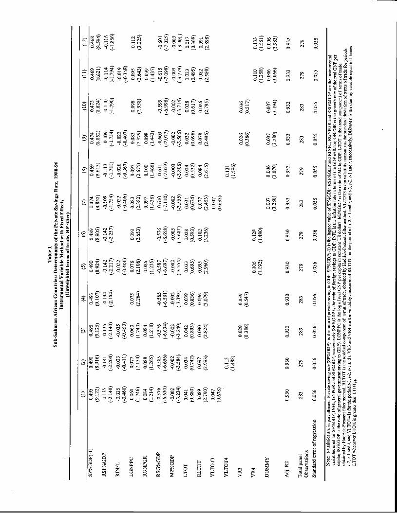
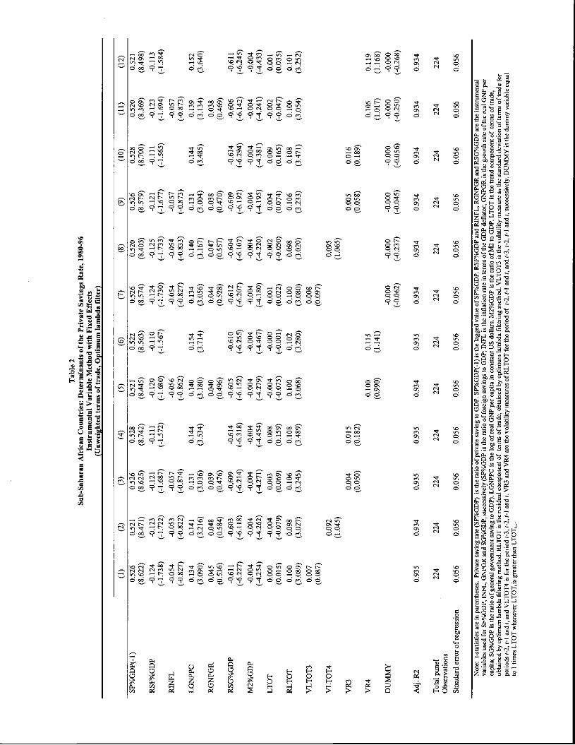
The regression results obtained for each of the filtering techniques de-scribed above, using two measures of the terms of trade (weighted and un-weighted) are summarized in Tables 1 to 12. Each table presents a series ofregressions with various sets of explanatory variables.9 Tables 1 to 6 use the
9The age dependency ratio turned out to have systematically the wrong sign in most
13

dummy variable for asymmetric shocks defined as one times the permanentcomponent of the terms of trade if there is a positive increase in that compo-nent between two years and zero otherwise; Tables 7 to 12 define the dummyvariable as one times the permanent component of the terms of trade if thereis a positive increase in that variable above the mean by at least one within-sample standard deviation and zero otherwise. In addition, Tables 1 to 3 usean unweighted terms-of-trade index and use the three alternative methods(standard HP, optimal HP, and nonparametric techniques) to calculate thepermanent and transitory components of the terms of trade, whereas Tables4 to 6 use a weighted index of the terms of trade, with weights given bythe ratio of exports over output for each country. Similarly, Tables 7 to 9(respectively 10 to 12) deal with unweighted (respectively weighted) data onthe terms of trade.
Consider first Tables 1 to 6. Overall, the adjusted R-squared is quitehigh, indicating that the regression model explains fairly well movements inthe private savings rate across countries and over time. The lagged depen-dent variable is highly significant, indicating (as noted earlier) either gradualadjustment to the desired level of saving or persistence effects associatedwith habit formation. Per capita income is also significant and positive (asexpected), whereas the growth rate of output, while having the correct sign,does not appear to have a discernible effect on private savings. The coef-ficient of the inflation rate is not well determined (its sign changes acrossregressions) and is never significant. This may reflect the importance oflow-inflation, CFA Franc countries in the sample. Foreign savings has a sig-nificant and negative impact on private savings, although the results appearto be weaker when the nonparametric filter and unweighted terms of trade areused. Government savings has a highly significant negative effect on privatesavings, as found in many recent studies on developing countries; govern-ment dissavings and their future tax implications tend to be internalized byprivate agents. The short-term coefficient of that variable is around 0.6; thecoefficient of the lagged variable is about 0.5, which gives a long-term coeffi-cient of 1.2 that is not significantly different from unity. This suggests thatRicardian Equivalence does hold in the long run, in contrast to the resultsfound by some recent studies. The index of financial development (the ratioof the broad money stock to GDP) has a highly significant and negative effect
regressions and often tended not to be significant. It was thus omitted from the resultsreported here.
14
on private savings; as noted earlier, this result is consistent with the viewthat financial liberalization may be accompanied by a relaxation of domesticliquidity constraints (increased access to bank credit, for instance), whichmay stimulate consumption and reduce the propensity to save.
The index of volatility of the terms of trade measured by the standarddeviation of the actual itself performs poorly in most regressions regardlessof whether three or four lagged values are used. The index based on thetransitory component of the terms of trade only does not perform muchbetter, except when the standard HP ifiter and weighted terms of tradeare used (regressions (9) to (12), Table 4). In these regressions, volatilityhas a positive effect on saving, as found for instance by Ohosh and Ostry(1994). As predicted by the consumption-smoothing view, the permanentcomponent of the terms of trade is nowhere significant. By contrast, thetransitory (cyclical) component is everywhere significant and has the rightsign, also as predicted by consumption smoothing considerations. However,the short-term coefficient of that variable is around 0.1 whereas the long-term value is around 0.2; both of these values are significantly different fromunity, suggesting that the "pass-through" is less than complete—perhapsbecause households are unable (even in the long run) to assess fully thedegree of persistence of terms-of-trade shocks at the moment they occur. Thedurmny variable that captures the asymmetric effect of terms-of-trade shocksis significant at a 1 percent level when the standard HP filter is used, withboth weighted and unweighted measures of the terms of trade. By contrast,with the optimal HP filter, the variable is not significant with unweightedterms of trade and is significant at only a 10 percent level when weightedterms of trade are used. With the nonparametric filter, the variable is alsosignificant at a 10 percent level and has the correct sign, regardless of whetherthe terms of trade are weighted or not.
Consider now Tables 7 to 12, in which regressions are based on the sec-ond measure of asymmetric shocks discussed earlier. The sign of the controlvariables are very similar to those obtained previously and to save space in-terpretations are not repeated here. Regarding the terms of trade variables,similar results also emerge: the index of volatility has a discernible effecton private savings only when the standard HP filter and the weighted termsof trade are used, and the coefficient of the permanent component of theterms of trade is not significantly different from zero. The dummy variablecapturing the asymmetric impact of improvements in the permanent compo-nent of the terms of trade is highly significant when the HP filter iä used,
15
with both weighted and unweighted measures. That is also the case with theoptimal HP filter—albeit significance levels are lower with weighted terms oftrade. With the nonparametric filter, the dummy variable is significant (at a5 percent level) with unweighted terms of trade and not significant (althoughwith the correct sign) when the terms of trade weighted by the share of ex-ports in output are used. Thus, the overall conclusion from the regressionresults presented here is that favorable movements in the permanent compo-nent of the terms of trade tend to have the asymmetric effect hypothesizedearlier on private savings. The use of a series of control variables, weightedand imweighted terms of trade, three different detrending techniques, andtwo different ways of measuring "favorable" disturbances give some degreeof robustness to the results.
5 Concluding RemarksThe purpose of this paper has been to examine whether terms-of-trade shockshave an asymmetric effect on private savings. The first part used a simplethree-period framework to argue that, in the presence of binding borrowingconstraints in bad states of nature, savings rates can be sensitive to favorablemovements in the permanent component of the terms of trade—in contrastto what the conventional consumption-smoothing framework would predict.Households in developing countries (particularly those that have limited cred-itworthiness to begin with) may indeed be unable to smooth consumption inthe face of adverse shocks to world commodity prices and the terms of trade,because they are subject to credit constraints that become more binding insuch situations. As a result, to maintain a smooth consumption path, do-mestic agents may be forced to dissave by a larger amount than they wouldotherwise when faced with a significant deterioration in their terms of trade.This argument also suggests that, to the extent that domestic agents in-ternalize the possibility of facing tighter credit constraints in bad states ofnature, they may also consume less and save more in good times.
The second part described the econometric methodology and the em-pirical specification of the model, which controls for various standard de-terminants of private savings. The third part presented and discussed theregression results, based on panel data for non-oil commodity exporters ofsub-Saharan Africa covering the period 1980-96. Overall, they suggest thattransitory movements in the terms of trade have a positive effect (albeit less
16
than one to one) on the propensity to save and that increases in the per-manent component of the terms of trade (measured using three alternativedetrending techniques and with both weighted and unweighted measures ofthe terms of trade) tend indeed to lead to higher rates of private savthgs.
Our interpretation focused on the adjustment of saving to a permanentshock, in circumstances where borrowing constraints are anticipated to bindin the future. It should be noted, however, that the empirical results maybe consistent with another interpretation. For example, if the permanentshock is associated with an anticipated increase in future volatility, it wouldraise the demand for assets needed to be used as an effective buffer stock inthe future, increasing thereby saving today. Nevertheless, it can be verifiedthat the logic of our analysis continues to apply in this case—the increasein the demand for the buffer stock is magnified by the anticipation of futureborrowing credit constraints and by greater loss aversion.
The analysis developed in this paper can be extended to study the asyrn-metric effects of terms-of-trade shocks on saving to oil-exporting countriesand analyze the response of public savings as well.10 This is important be—cause of the policy concerns that the high degree of commodity price volatilityhas generated in recent years. The 1998 slump in commodity prices, for in-stance, generated large terms-of-trade effects. Although the real income effecton primary commodity exporters was moderate (of the order of-0.5 percent ofGDP), and net importers of oil and primary commodities actually registereda gain overall, oil exporters registered a negative real income effect of theorder of -6.3 percent of GDP (World Bank (2000, Chapter 4)). Because oilexports account for almost all of government revenues in oil-exporting coun-tries, the public sector bore the brunt of adjustment. The ability of eachcountry to smooth public consumption in response to the revenue shortfallwas, however, limited by their ability to draw down their official reservesand to borrow, both domestically and abroad. In many cases, constraintson domestic finance and lack of access to international capital markets ac-tually prevented governments from successfully smoothing the impact of theoil price cycle, and economic performance deteriorated." The same study by
'°An early study that attempted to test for an asymmetric effect of terms-of-trademovements on savings in oil-exporting countries is by Spatafora and Warner (1995). How-ever, the test poerformed by the authors was essentially a standard stability test of thecoefficient of the terms-of-trade variable across two sub-periods (1965-80 and 1981-89).
1'The World Bank report estimated that the effect of the drop in oil prices on theexternal earnings of oil-exporting countries in sub-Saharan Africa led to a deterioration in
17
the World Bank also noted that although adjustment to the oil price swingsin the past few years differed significantly across oil exporters, most countriesincreased their aggregate saving rates during the rise in oil prices in 1996-97 (compared to 1993-95) and reduced them during the 1998 slump. Thispattern is consistent with consumption smoothing behavior in the presenceof perceived transitory shocks, In addition, the savings response was foundto be asymmetric: on average, savings rates rose by less than half of thereal income gain during the 1996-97 boom, but fell by the full amount ofthe decline in real incomes during the 1998 collapse in prices. Extending theanalytical framework presented in this paper to account for an asynunetricresponse of public savings along these lines would provide a fruitful exercise.
the fiscal balance of these countries of about 7 percent of GDP in 1998.
18
Appendix ALoss Aversion, Savings, and Borrowing Constraints
The purpose of this Appendix is to show that, following Aizenman (1998),loss aversion magnifies the increase th saving induced by the anticipation offuture binding borrowing constraints induced by adverse shocks to income.
For expositional simplicity, we will assume the absence of habit formation,that is, the case in which = U = 0 in equation (2). Loss aversion modifiesthe maximization problem with full access to the capital market given in (4)as follows:
f n(x — si) + (w + q)[u(x —8 + si — 4) + u(x + 4)] Al+(l - q - w)[u(x + s - s') + u(x + $)J
where to simplify notations, u(ci; c±) is written as u(ct) and 1— q � w � 0.The term w is the extra utility weight attached to the bad state of naturedue to loss aversion (see Aizenman (1998) for further details). The expectedutility case corresponds to w = 0. With no access to the capital market, themaximization problem (9) becomes
I u(x —81) + (w + q)[u(x —8 + Si) + u(x)]maxs H H 2
(l—q—w)[u(x+si—s2)+u(x+s2)
Applying (Al) if follows that with access to the world capital market,first-period savillg is
8(q+w)(A3)
whereas without access to borrowing and with no habit formation, saving is
— 8(q+w) A42— 0.5[l — (q + w)j
Ftom (A3) and (A4), we have
8(q+w)(3—q—w)Si — Si —
3(3+q+)Consequently, loss aversion magnifies the increase in saving associated
with future borrowing constraints.
19

Appendix BCountries, Variables, and Data Sources
This Appendix presents the list of countries included in the text andprovides a more precise definition of the variables used in the regressions(including the dummy variables) shown in Tables 1 to 12.
The sample used in this study includes all sub-Saharan African coun-tries except oil exporters. Specifically, the list of the countries consists ofBenin, Botswana, Burkina Fa.so, Burundi, Cameroon, Cape Verde, CentralAfrican Republic, Chad, Comoros, Democratic Congo, Cote d'Ivoire, Dji-bouti, Eritrea, Ethiopia, Gambia, Ghana, Guinea, Guinea-Bissau, Kenya,Lesotho, Liberia, Madagascar, Malawi, Mali, Mauritania, Mauritius, May-otte, Mozambique, Namibia, Niger, Rwanda, Sao Tome and Principe, Sene-gal, Seychelles, Sierra Leona, Somalia, South Africa, Sudan, Swaziland, Tan-zania, Togo, Uganda, Zambia, and Zimbabwe.
The variables used in the regressions reported in Tables 1 to 12 are definedas follows.
• Private saving, SP%GDP: The ratio of private saving to GDP. It isobtained as the difference between Gross Domestic Saving and Gov-ernment Saving. The gross domestic saving is defined as the differencebetween gross domestic product and total consumption. Source: theWorld Bank's Statistical Information Management and Analysis Sys-tem (SIMA).
• Foreign saving, SF9oCDP: Ratio of foreign saving to GDP. Foreignsaving is equal to the current account surplus, which is defined as mi-nus the sum of net exports of goods and services, income and currenttransfers. Source: SIMA.
• Residual foreign saving, RSF%CDP: obtained by regressing foreignsaving on the log of the terms of trade weighted by the ratio of realexports to real GDP, an index of terms-of-trade volatility, the log ofreal GNP per capita, and the rate of change in the ratio of broad moneyto GDP.
• Inflation, INFL: growth rate of GDP Deflator. It is calculated byusing GDP in current and constant 1987 local currency prices. Source:World Development Indicators (WDI).
20

• Residual inflation, RINFL: Obtained by regressing inflation on thelog of the terms of trade weighted by the ratio of real exports to realGDP, an index of terms-of-trade volatility, the log of real GNP percapita, and the rate of change in the ratio of broad money to GDP.
• Log of real GNP per capita, LGNPPC: gross national product (inconstant 1995 U.S. dollars) divided by midyear population. Source:WDT.
• Real GNP per capita growth rate, GNPGR: growth rate of real GNPper capita. Source: WDI.
• Residual Real GNP per capita Growth Rate, RGNPGR: obtainedby regressing real GNP per capita on the log of the terms of tradeweighted by the ratio of real exports to real GDP, an index of terms-of-trade volatility (as defined above), the log of real GNP per capita,and the rate of change in the ratio of broad money to GDP.
• Government Saving, SG%GDP: ratio of government saving to GDP.Government saving is defined as the difference between tax revenue andgeneral government consumption. General government consumptionincludes all current expenditures for purchases of goods and servicesby all levels of government, excluding most government enterprises. Italso includes capital expenditure on national defense and security. Taxrevenue comprises compulsory, unrequited, nonrepayable receipts forpublic purposes collected by central governments. Source: SIMA.
• Residual government saving, RSG%GDP: obtained by regressing gov-ernment saving on the logarithm (log) of the terms of trade weightedby the ratio of real exports to real GDP, an index of volatility of theterms of trade (as defined below), the log of real GNP per capita, andthe rate of change in the ratio of broad money to GDP.
• Trend component of terms of trade weighted by ratio of real exportsto real GDP, RLTOT: obtained through the three filtering methodsdescribed in the text. The terms of trade used in this study are definedas the log of the terms of trade unweighted and weighted by the ratioof real exports of goods and services to real GDP. The terms of tradefor goods and services are the ratio of the export price index to the cor-responding import price index (with base 1995=100). Real exports of
21

goods and services and real GDP are defined in constant local currencyunits. Source: SIMA.
• Residual (temporary) component of terms of trade weighted by ratioof real exports to real GDP, RLTOT: The residual component of theterms of trade is calculated as the difference between the (weighted orunweighted) terms of trade and LTOT.
• Index of terms-of-trade volatility, VLTOT3: equal to the standarddeviation of the log-difference of the terms of trade for periods t, t —1
and t — 2.
• Index of terms-of-trade volatility, VLTOT4: equal to the standarddeviation of the log-difference of the terms of trade for periods t, t —1,t — 2 and t —3.
• Index of terms-of-trade volatility. VR3: equal to the standard deviationof the log-difference of the residual component of weighted terms oftrade for periods t, t — 1 and t — 2, using each alternative filter.
• Index of terms-of-trade volatility, VR4: equal to the standard deviationof the log-difference of the residual component of weighted terms oftrade for periods t, t — 1, t — 2 and t — 3, using each filter alternativefilter.
• DUMMY: dummy variable equal to 1 times LTOT for period t when-ever LTOT is greater than LTOT1 and 0 otherwise.
• DUMMY2: dummy variable equal to 1 times LTOT for period t when-ever LTOT is greater than the mean value of LTOT plus at least onestandard deviation of LTOT, and 0 otherwise.
22
References
Agenor, Pierre-Richard, The Economics of Adjustment and Growth, AcademicPress (San Diego, CA: 2000).
Agenor, Pierre-Richard, C. John McDermott, and Eswar Prasad, "Macroeco-nomic Fluctuations in Developing Countries: Some Stylized Facts," unpub-lished, the World Bank (January 1998). Forthcoming, World Bank EconomicReview.
Agenor, Pierre-Richard, and Peter J. Montiel, Development Macroeconomics,Princeton University Press, 2nd ed. (Princeton, New Jersey: 1999).
Aizenman, Joshua, "Buffer Stocks and Precautionary Savings with Loss Aver-sion," Journal of international Money and Finance, 17 (December 1998),931-47.
Alessie, Rob, and Anna Maria Lusardi, "Consumption, Saving and Habit For-mation," Economics Letters, 55 (August 1997), 103-8.
Bevan, David, Paul Collier, and Jan W. Gunning, "Trade Shocks in Develop-ing Countries: Consequences and Policy Responses," European EconomicReview, 37 (April 1993), 557-65.
Cashin, Paul, and C. John McDermott, "Terms of Trade Shocks and the Cur-rent Account," Working Paper No. 98/177, International Monetary Fund(December 1998).
Cogley, Timothy, and James M. Nason, "Effects of the Hodrick-Prescott Filteron Trend and Difference Stationary Time Series: Implications for BusinessCycle Research," Journal of Economic Dynamics and Control, 19 (January1995), 253-78.
Collier, Paul, and Jan W. Gunning, "Trade and Development: Protection,Shocks and Liberalization," in Surveys in International Trade, ed. by DavidGreenaway and L. Alan Winters, Basil Blackwell (Oxford: 1994).
Deaton, Angus S., Understanding Consumption, Oxford University Press (Ox-ford: 1992).
Deaton, Angus S., and Guy Laroque, "On the Behaviour of Commodity Prices,"Review of Economic Studies, 59 (January 1992), 1-23.
Devereux, John, and Michael Connolly, "Commercial Policy, the Terms of Tradeand the Real Exchange Rate Revisited," Journal of Development Economics,50 (June 1996), 81-99.
Edwards, Sebastian, "Temporary Terms-of-Trade Disturbances, the Real Ex-change Rate and the Current Account," Economica, - (- 1989), 343-57.
23
Elbadawi, Ibrahim, and Francis Mwega, "Can Africa's Saving Collapse be Re-verted?," in The Economics of Saving and Growth, ed. by Klaus Schmidt-Hebbel and Luis Serven, Cambridge University Press (Cambridge: 1999).
Gavin, Michael, "Structural Adjustment to a Terms of Trade Disturbance: TheRole of Relative Prices," Journal of International Economics, 28 (May 1990),.217-43.
Ghura, Dhaneshwar, and Michael Hadjimichael, "Growth in sub-Saharan Africa,"IMF Staff Papers, 43 (September 1996), 605—34.
Greene, William H., Econometric Analysis, 3rd. edition, Prentice Hall (UpperSaddle River, New Jersey: 1997).
Harberger, Arnold C., "Currency Depreciation, Income and the Balance of'liade," Journal of Political Economy, 53 (February 1950), 47-60.
Hubbaid, R. Glenn, and Kenneth L. Judd, "Liquidity Constraints, Fiscal Policy,and Consumption," Brookings Papers on Economic Activity, 1 (June 1986),1-50.
King, Robert G., and Sergio Rebelo, "Low Frequency Filtering and Real BusinessCycles," Journal of Economic Dynamics and Control, 17 (January 1993),207—31.
Laursen, Svend, and Lloyd A. Metzler, "Flexible Exchange Rates and the Theoryof Employment," Review of Economics and Statistics, 32 (November 1950),281-99.
Loayza, Norman V., Luis Serven, and Klaus Schmidt- Hebbel, "What DrivesSaving across the World?," in The Economics of Saving and Growth, ed. byKlaus Schmidt-Hebbel and Luis ServOn, Cambridge University Press (Cam-bridge: 1999).
Obstfeld, Maurice, "Aggregate Spending and the Terms of Trade: Is there aLaiirsen-Metlzer Effect?," Quarterly Journal of Economics, 47 (May 1982),251-70.
Obstfeld, Maurice, and Kenneth A. Rogoff, Foundations of International Macro-economics, MIT Press (Cambridge, Mass.: 1997).
Ogaki, Masao, Jonathan Ostry, and Carmen M. Reinhart, "Saving Behavior inLow- and Middle-Income Developing Countries: A Comparison," IMP StaffPapers, 43 (March 1996), 38-71.
Ostry, Jonathan D., and Carmen M. Reinhart, "Private Saving and Terms-of-Trade Shocks," IMP Staff Papers, 39 (September 1992), 495-517.
Seater, John, "Ricardian Equivalence," Journal of Economic Literature, 31 (March1993), 142-90.
24
Spatafora, Nikola, and Andrew Warner, "Macroeconomic Effects of Terms ofTrade Shocks," PRE Working Paper No. 1410, the World Bank (January1995).
Svensson, Lars, and Assaf Razin, "The Terms of Trade and the Current Account:The Harberger-Laursen-Metizer Effect," Journal of Political Economy, 91(February 1983), 97-125.
World Bank, Global Development Finance 1999, the World Bank (WashingtonDC: 1999).
Global Economic Prospects and the Developing Countries 2000, the WorldBank (Washington DC: 2000).
Zeldes, Stephen, "Consumption and Liquidity Constraints: An Empirical Tnsves-tigation," Journal of Political Economy, 97 (April 1989), 305-46.
25

Figure 1Non-Oil Sub-Saharan Africa:
Volatility of Output and the Terms of Trade(Averages for 1980-96)
0.35 -
.03 •
0o 025 -o(Ua) S:: 0.2- So S2' • a
0.15- •• • V .> ••
0.1- S
—a S0.05- • C SS
00.00 0.05 0.10 0.15 0.20
Volatility of the terms of trade (weighted)
0.35 -
S0.3- 55
0O 0.25 -
0m, 0.2- 5
S S0.15- • •••. • Si
> - Si •S.0.1 — S
SS S0.05- .% ..
0 I I
0.00 0.01 0.02 0.03 0.04 0.05 0.06 0.07 0.08
Volatility of the terms of trade (unweighted)
Source: World Bank.
Note: Volatility is measured by the coefficient of variation over the whole sample period.1/List of the countries: Berm, Bostwana, Burkina Faso. BurLindi, Cameroon, Cape Verde, Central African Republic,Chad, Comoros, Congo Democratic Republic, Ethopia, Gambia, Ghana, Guinea. GuineaBissau, Kenya, Lesotho,Madagascar, Malawi, Mali, Mauritania, Mauritius, Mozambique, Namibia, Niger, Rwanda, Sao Tome and Principe,Senegal, Seychelles, Sierra Leone, South Africa, Swaziland, Tanzania, Toga, Uganda, Zambia. Zimbabwe.
Tab
le I
S
tab-
Sah
aran
Afr
ican
Cou
ntrie
s: D
eter
min
ants
of th
e P
rivat
e S
avin
gs R
ate,
198
0-96
In
stru
men
tal
Var
iabl
e M
etho
d w
ith F
ixed
Effe
cts
(Unw
eigh
ted
term
s of t
rade
, III'
filte
r)
(1)
(2)
(3)
(4)
(5)
(6)
(7)
(8)
(9)
(10)
(i
i)
(12)
SP%GDP(-I)
0.495
0.490
0.495
0.493
0.490
0.489
0.474
0.469
0.474
0.473
0.469
0.468
(9.1
22)
(8.9
16)
(9.1
25)
(9.1
07)
(8.9
24)
(8.9
05)
(8.8
52)
(8.6
13)
(8.8
52)
(8.8
24)
(8.6
21)
(8.5
94)
RSF
%G
DP
-0.1
35
(-2.
140)
-0
.141
(-
2.20
4)
-0.1
35
(-2.
140)
-0
.134
(-
2.15
4)
-0.1
42
(-2.
217)
-0
.142
(-
2.25
7)
-0.1
09
(-1.
754)
-0
.113
(-
1.78
1)
-0.1
09
(-1.
754)
-0
.110
(-
1.79
0)
-0.1
14
(-1.
794)
-0.1
16
(-1.
856)
R
INFL
-0
.025
(-
0.46
1)
-0.0
23
(-0.
411)
-0
.025
(-
0.46
0)
-0.0
22
(-0.
401)
-0
.022
(-
0.40
6)
-0.0
20
(-0.
367)
-0
.022
(-
0.40
7)
-0.0
19
(-0.
358)
L
GN
PPC
0.
061
(1.7
46)
0.07
7 (2
.134
) 0.
060
(1.7
40)
0.07
5 (2
.264
) 0.
076
(2.1
06)
0,09
1 (2
.653
) 0.
083
(2.3
82)
0.09
7 (2
.675
) 0.
083
(2.3
79)
0.09
8 (2
.938
) 0.
095
(2.6
43)
0.11
2 (3
.225
) R
GN
PGR
0.
084
(1.2
14)
0.08
8 (1
.265
) 0.
084
(1.2
18)
0.08
6 (1
.235
) 0.
097
(1.4
36)
0.10
0 (1
.466
) 0.
098
(1.4
43)
0.09
9 (1
.437
) R
SG%
GD
P -0
.576
(-
6.63
0)
-0.5
83
(-6.
656)
-0
.576
(-
6.60
4)
-0.5
65
(-6.
561)
-0
.587
(-
6.69
7)
-0.5
76
(-6.
658)
-0
.610
(-
7.11
0)
-0.6
11
(-7.
059)
-0
.609
(-
7.07
7)
-0.5
95
(-6.
996)
-0
.615
(-
7.09
8)
-0.6
01
(-7.
025)
M
2%G
DP
-0.0
02
(-3.
234)
-0
.002
(-
3.58
4)
-0.0
02
(-3.
240)
-0
.002
(-
3.39
2)
-0.0
02
(-3.
554)
-0
.003
(-
3.68
2)
-0.0
02
(-3.
555)
-0
.003
(-
3.80
8)
-0.0
02
(-3.
566)
-0
.002
(-
3.71
4)
-0.0
03
(-3.
779)
-0
.003
(-
3.90
1)
LT
OT
0.
04!
(0.8
80)
0.03
4 (0
.742
) 0.
042
(0.8
93)
0.03
9 (0
.836
) 0.
033
(0.6
95)
0.02
8 (0
.593
) 0.
031
(0.6
74)
0.02
4 (0
.532
) 0.
032
(0.6
96)
0.02
8 (0
.617
) 0.
023
(0.4
95)
0.01
7 (0
.369
) R
LT
OT
0.
089
(2.7
90)
0.09
7 (2
.993
) 0.
090
(2.8
24)
0.09
6 (3
.079
) 0.
095
(2.9
60)
0.10
2 (3
.236
) 0.
077
(2.4
53)
0.08
4 (2
.615
) 0.
078
(2.4
95)
0.08
6 (2
795)
0.
082
(2.5
80)
0.09
1 (2
.898
) V
LT
OT
3 0.
047
(0.6
78)
0.04
7 (0
.693
) V
LT
OT
4 •
0.11
5 (1
.488
) 0.
321
(1.5
96)
VR
3 0.
029
(0.3
86)
0.03
9 (0
.547
) 0.
026
(0.3
66)
0.03
6 (0
.517
) V
R4
0.10
6 (1
.192
) 0.
428
(1.4
80)
0.11
0 (1
.258
) 0.
133
(1.5
61)
DU
MM
Y
0.00
7 (3
.280
) 0.
006
(3.0
70)
0.00
7 (3
.280
) 0.
007
(319
4)
0.00
6 (3
.066
) 0.
006
(2.9
83)
Adj
. R2
0.93
0 0.
930
0.93
0 0.
930
0.93
0 0.
930
0.93
3 0.
933
0.93
3 0.
932
0.93
3 0,
932
Tot
al pa
nel
283
279
283
283
279
279
283
279
283
283
279
279
Obs
erva
tions
Stan
dard
err
or o
f reg
ress
ion
0.05
6 0.
056
0.05
6 0.
056
0.05
6 0.
056
0.05
5 0.
055
0.05
5 0.
055
0.05
5 0.
055
RSF
%G
DP
and R
INE
L. R
GN
PGR
and
RSG
%G
DP
are
the
inst
rum
enta
l N
ote:
t-s
tatit
tics
are
in pa
rent
hese
s, P
riva
te sa
ving
rat
e (S
P%G
DP)
is
the
ratio
of p
riva
te s
avin
g to
GD
P. S
P"/o
OD
P(-I
) is th
e la
gged
val
ue o
fSP%
00P.
va
riab
les
used
for S
F'/G
GD
P,
fl'4
fL, G
NPG
R a
nd SG
%G
DP,
suc
cess
ivel
y (S
F%G
DI'
is th
e ra
tio o
f for
eign
sav
ings
to G
DP;
INFL
is
the
infl
atio
n ra
te in
tenn
a of
the
OD
P de
flat
or; G
NI'G
R i
s th
e gr
owth
rat
e of
the
real
GN
P per
ca
pita
; S0
%G
DP
is t
he ra
tio o
f gen
eral
gov
ernm
ent s
avin
g to
GD
P). L
GN
PPC
is
the
log
of re
al O
N? p
er ca
pita
in
cons
lant
US
dolla
rs.
M2%
GD
P is
the
ratio
of M
2 to
OD
P. L
TO
T a
the
tren
d co
mpo
nent
of
teem
s of
tTad
e,
obta
ined
by
Ilod
rick
-Pre
seot
t fi
fter
mel
hod.
RL
TO
T is
the
resi
dual
com
pone
nt o
f te
rms
oftr
ade,
ohta
ined
by
Hod
rick
-Pre
scot
t filt
er m
etho
d. V
LT
OT
3 is
the
vola
tility
mea
sure
as
Ihe
stan
dard
dev
iatio
n of
term
s oft
rade
forp
erio
da
1-2,
1-1
and
t, an
d VL
TO
T4
is f
orth
cper
iodi
-3, 1
-2, c
-I a
nd t.
VR
3 an
d VR
4 ar
ethe
vol
atili
tym
easu
reso
fkL
TO
T fort
hcpe
riod
of t-
2, i-
I an
d!, a
nd 1-
3, (
-2, I
-I a
nd t.s
ucce
ssiv
ely.
DU
MM
Y i
s th
e du
mm
yvar
iabl
e eq
ual t
o I tin
es
LT
OT
whe
neve
r L
TO
T, it
grea
ter
than
LT
OT
11.
-171011 ug41 aoinoa2 S! LO
Ll loA
ourn]M 1011
7 01
1rnbo 1qfluvA (w
Lnnp 041
Aw
i!nu &
IaMss000rIs ;puw
7-; 'i—; g-;puE
'7 puE
7-J 'i-; jopouodoqiio; jØj)JJ0 sainsE
Om
A
PI1IEIO
AO
MI
3m p)JA
puw cJ)Jp,
pu t-;'z- 's-; pouodoipaoj 7! 101lA puP ';p'm
7-; 'i-; spouod IO
J OpP11J0 1U
1J01J0 UO
ilflAO
P PiPPUPiS 04127
OJflSB
OL
U A
1!II1EI0 042 S
i £JOflA
p0410w 8U
U0111J opqw
j wnw
Sldo Aq pO
UiE
IqO O
pRJlJo SU
u3 JO luouodw
oo IEnP!101 0455! .L
0L1M
P0423W
2U7l31(IJ E
P4WSI w
nui!ldo £4 paurnqo apSJ1Jo 511001 Jo luouodw
oo P0351 0415! LO
ll dUO
01 ZN
J0 07171 34177 dUO
%Z
N
SmII0P Sf1107151100 117 1!3 10d dM
0 j0J0 2Oj 0415! D
ddMO
l (auo 01 SUIA
?S 1U
DIU
UJO
AO
S jeirnso8jo 01121 45 71 dUO
%O
S 7l!d50 nd dN
O 7501 041 JO
3571 4w012 341 SV
0dN0 JO
I5UO
PdQO
O4IJO
SUU
OSU
! 0751 U
0!ICIJU
! 3455! 1JN1 JQ
O 05 52U
!A5S U
!3JOJJO
0515104157 dUO
%dS)X
IOA
!55300fl5 'dU
O%
0S PU
? 10dNO
14M 'dU
O%
4SJOJ pO
Sfl SO
74SUSA
I7IUO
SUT
UISU
! 041 015dU0%
OSPu5aO
dNO
H 1JN
N P115 dU
0%JS1I dU
O%
d8J03n15t 055 0(11 ! (l-)aao%as dU
O o12uiA
ss olsAudjo osIcioqIss
(duo%ds)31512u!A
ss O
N41d
sasoqiuomdus 3m
5311si1715-1 :oloN
(89t1) (L
ToT
) 6110
coto (6810)
(scot) 9100
cooo (c9o1) c600
9c00 uoissai2oijo 10110 pnpuo
SUO
!1PAJO
sqo I'll
1-11 1-11
I'll loundlelol
(i-ii) (0660)
ci to auja
(zsto) (ocoo)
ciot t-ooo
ccoo ni Ipv
9cc-u
1-li 1-11
t'll 1-11
1-11 1-11
t'E60
1-E60
1-EG
O
1-E60
PE6O
(89ro-) (octo-)
(9coo-) (ct'oo-)
(Lao-)
(1900-) 000•0-
000-0- 000•0-
0000- 0000-
0000-
900 9c00
900 9c0O
9c00
9c00 900
9ç0O
9c00 9c0a
cE60
t'E60
c€6o cE
6o
(L6oo) 8000
(lczE)
(t'co€) ([L
YE
) (€at)
(aloE)
(osoi) 1010
0010 SO
lO
9070 8600
0010 (cE
o-c) (L
P0-o-) (c91-o)
(no-u) 1000
1000- 6000
1-000 (€ttr)
(11-tv—)
(78Ev—
) (c61p—
) 1-000'
1-00'O
t'OO
O-
1-000-
'-€6.0
(ct-oi) 1600
(Lso'o)
L00.0
(o8rE)
(890€) (681€)
(ct-CE
) (aoU
(680€)
1010 0070
SOlO
9010
8600 0070
(tuou-) (cL
oo-) (6c1u)
(6900) 000,0
t00'O
8000 £000
(L91-'t--)
(6L1's—
) (t-ct-'i-—
) (itrr)
toot- toot-
too'o- *000-
(cvz9-) (zvt9-)
1190- 9090- (691-0) S £00
(ocuo-) 1000'
(oat—)
t-000- (L
a 1'9) t'09'0
(tcc'o) L
t'OO
(v6r9-) (1619-)
1-190- 6090- (ott-a) 8 £00
(1100) 1000
(osit--) 1-00'O
-
(ton-) 1190-
(szc'o) "pa-c
(EL 80-)
tco'o- (s-sc'i-)
(1-691-) £110-
Ella-
(ccl'9-) (lcl'9-)
0190 c090-
(961-u) 01-00
(o*9c) (t-E
I'E)
(cst-'E)
(tau'€) (L
91'E)
(9coE)
(s-rt'€) (osr'€)
(tEcE
) (9E
aE)
(911€) (060€)
zcio 600
flI'O
[€10 onu
1-Etc
tcIa 01-to
1-Plo lE
LO
11-10
1-E1O
(oLao-)
1-0 O'O
-
(19Cr-)
1-0 00- (8 11-9-) £090- (t-sco) 81-0_c
(81E9-)
(*119-) 1-190-
6090- (9L
1u) 6 £00
(cia-u) 000'O
(1-cry-) 1-000-
(L1r9-)
1790-
(9Eco)
ctoo
AN
INflO
EU
A
I-lofl&
£lOrL
&
1OlD
!
L01l
dUO
%Z
F'J
dcIO%
OS)1
1OdN
tTh
3ddME
fl
dUD
%r1S
(asu-) (c€so-)
(aso-) (1980-)
(nsa-) (asa-)
Lcuo-
i-coo- i-coo-
cao- L
coa- €cco-
(c9cl-) (L
L9l-)
(cai-) (ccci-)
(L9c1-)
(0891-) (act-)
(L89i-)
(zai-) 1110-
1110- lU
0- 1-110-
0110- 0110-
1110 1110-
£110- (861-8)
(69(5) (oots)
(6tcs) (cops)
(ncs) (c9cs)
(ct-is) (rt-cs)
(c19S) (itvs)
(1198) 1co
ozc-c szca
91ca 0l0
91cc aco
lco szco
91cc IlcO
91cu
(i -)duo%ds
(zi) (it)
(ot) (6)
(s) (t)
(9) (c)
(t-) (c)
(z) (I)
(Jallu vpqmuj m
nmgdo 'apuiI Jo S
Wfl4 paiq7aM
ufl)
(aso-) vcou-
(scci-) 1-110-
S;O
aJJ paX!J IfliM
poq;aj ajqrnJ7 isiuamnijsui
96-086! 'a3flj s2U!A
ss aJvA71J aq;jo sutujm
iaiau :sau3uno3 us3!iJy uvnqsg-qn5

1-11011 UC
4I loiniS Si 1011 10AtU
4M 1011 sam
i 01
Itnba 0jqsIJs &uim
np 043 SI Apw
no XlaA
Issossns 7 put i-s 'z-; c-, put; put i-s z-; jo pouad
0131.103 10rm40 SO
InSIsaw A
iqi;rjo.& 045 am
fliA put £T
A
7 pus r-;'z-rc-; pouad aqi 104 si t'IoIjA. put; put 1-; -s spouad
104 OpR
lljO 511110340 uoijrnap prnpuniw
045 St O
lflStOU
l X1i1i3t1o
0533 Si £LO
J.]A pO
qpm 8u1.lslpJ zsupuiiusd-uou A
q pauiSlqo 'apIS
Iljo SuIJI3 JO
3uOuodm
OO
tupiS
al Oi3) S
i .L01Th poqlom
8tiuajij OLIllIrnutd-uou q pauitiqo
apluIjo suL
la3 Jo3unuodmon U
013 04) S Loll 1000) ZY
'IJ° 01351 053 Si duO%
ZIN
5J5110P SfllutltuoD
U!tl!dtO
ThddN
o 1t1140 80 0418! DddN
Ol (duo 038U
1/t583110111U10408
I"J° 01tfll31 ! dU05/oO
S tt,dto iad dM
0 I'm-' 04)jO
0351 q3MO
1 0133 Si ?103N
0 !lOltIjtp duo 31340 50003
Ui 351 U
OiJtIJIIi 43 Si 14N
1 d0 03 ISUT
AE
S ulioojjo 01351 3435! duO%
dS) A1O
AT
SSOX
,ns 'duo%0S pU
t )A0JZ
0 1dM dU
O%
dS 104 posn sa)4SUSA
pquam
lulSut 3533 3.15 dGO
t/0OSN
llt MO
dNO
H '1dN
IHPU
O dU
O%
dSH
dGO
%dSJO
I5P0ZI 0431! (1-)dao%
ds dUO
03 5uiAss 33rA
udJo oqu aqi S (duo%
ds) D
3EI8U
1ASSO
3EA
1Id sataq3uaitd
U! 015 SD
!3S!IBIS-3
OIO
N
9c00 0015S01201J0 50110 PJE
PUP3S
SUoi1tA
10Sq vzz
jougdjuoj
ni - Ipv
9co-o 9c00
9coo 9c0o
9100 9100
9100 9100
9100
t'(60
(cooo) 1800
(19t0) tL0O
9100 9100
I-U
PU
P
U
PU
P
U
PU
1c60 1160
9160 1160
1160 1(60
160 1(60
1160 P
160 1(60
(ton) (89Ll)
(68L1) (T
nT)
(OIL-I)
(ocwi)
P000
P000
P000
P000
P000
P000
(1980) (tw
o) 0800
1900
(1110-) (zuo-)
(1100-) (P
600-) 000-
IWO
- 1000-
1000-
(8160) (110)
9800 1600
(noo-) (nto)
£000- 6000
(6101) (a9z)
(ssit) C
ast) (u.cz)
(tv9z) (nz)
(uoz) (zcv)
(Lzi) (988t)
(zcoz) lI0
(010 1110
6010 8600
010 R
IO
P110
LZI0
OZ
I0 600
tITO
(6600)
(ozo) P
000 0100
(9z9P-)
(tzv-) P
000 P
000
(o8v9-) (LLc.9-)
9190-
(89Lo) 1900
(1991) (tsoc)
9P10
1110
(I-plo-)
(olc t-) (n9 I-)
0110- 9110-
(oro) (6sro)
(o 10) (9zro)
(1100) (1910)
(oIl-c) (lI-to)
(ooio) 6000
P100
1000 1100
(000 8000
8000 Z
T00
1000
(p99p) (z9ptr-)
(t'6c-P-)
(86n'-) (nc-s—
) (sir—
) (IvcP-)
(6Prr-) C
oors-) P
000 t000
P000-
P000
tOO
0 P
000- P
000 P
000- P
000
(cPl-9)
(Lzt'9-) (ppy_)
(6zr9-) (clz9-)
(8€9-) (9cz-9-)
(1119-) 0P90
9190 0190-
6(90- U
90- 690-
1Z90-
0Z90-
1190-
(9890) (icso)
(911-0) (8P
9o) (9Lco)
(aco) 1100
6900 £900
zco_0 9P
00 6100
(ctc) (0101)
(ai€) (P
io€) (zz9)
(1801) (gocE
) (1101)
(zci€) IPIO
L
ZI0
1(10 8Z
10 9P10
ZO
O
UI-T
O
8Z10
L(t0 (96co-)
(solo-) (1110-)
(1110-) (stco-)
(coco-) 1(00-
1100- ((00-
£(00 9(00-
1(00- (9811-)
(1191-) (usj-)
(9691-) (0091-)
(P191-)
(1191-) (9191-)
(toci-) 0110-
8110- 6110-
OZ
I0- Z
110- 6110-
£1I0 0Z
I0 U
I0
AW
WflU
Pm'
Itt P
JLOflA
£.L0.L1A
iorni
IOn
dUO
%Z
W
dclO%
0Sa
80dND
I
DddN
Ol
ldNIU
dUO
%dSll
(soos) C
o 161) (I-Los)
(1161) (s'tst)
£010 zoco
soco oco
loco
(oslo) 6000
(zozP-) P000- (19r9) £Z
90-
(9990) P
100
(010-U
0(10 (izco-) £100-
(6111-) £1 10-
(ctot) (1598)
(6918) (9815)
(uv9s) (tocs)
(9c9s) £010
0(10 0(10
ZE
cO
zao szco
(EcO
(T
-)duo%as
(ti) (it)
(01) (6)
(s) C
t) (9)
Cc)
Cs)
(1) ()
(1)
(ia;jij a!l3amuJsd-U
0N 'apF
J; JO S
W1 pa;qT
haAtufl)
SJD
Ojfl p3X
11 IflM poipajç ajqE
1 W1uuIfl1*Sil1
960861 'ama S
iIAt5 O
3nA.Id 43JO
sIuuulwlam
aa :sa.luno UV
OIJJV
usicuv5-qn5 (aqB
I

Tab
le 4
Sub
-Sah
aran
Afr
ican
Cou
ntri
es: D
eter
min
ants
of th
e Pri
vate
Sav
ings
kale
, 19
80-9
6 In
stru
men
tal V
aria
ble
Met
hod
with
Eix
ed E
ffec
ts
(1)
(2)
(3)
(4)
(5)
(6)
(7)
(8)
(9)
(10)
(I
I)
(12)
SP
%G
DP(
-l)
0.45
9 0.
454
0.45
8 0.
461
0.45
3 0.
456
0.45
1 0.
446
0.45
1 0.
449
0.44
5 0.
444
(8.5
91)
(8.3
61)
(8.5
45)
(8.5
83)
(8.2
83)
(8.3
72)
(8.5
11)
(8.2
77)
(8,4
72)
(8.4
41)
(8.2
02)
(8.1
78)
RSF
%G
DP
-0.1
27
(-2.
066)
-0
.135
(-
2.16
3)
-0.1
27
(-2.
070)
-0
,135
(-
2.21
3)
-0.1
33
(-2.
147)
-0
.145
(-
2.36
0)
-0.1
27
(-2.
089)
-0
.133
-0
.127
(-
2.14
7)
(-2.
091)
-0
.128
(-
2.12
8)
-0.1
32
(-2.
138)
-0
.134
(-
2.19
2)
RIN
FL
-0.0
06
(-0.
107)
-0
.002
(-
0.04
1)
-0.0
11
(-0.
191)
-0
.006
(-
0.11
6)
-0,0
04
(-0.
085)
-0
.003
-0
.009
(-
0.05
0)
(-0.
165)
-0
.006
(-
0.10
6)
LG
NPP
C
0.08
0 (2
.352
) 0.
086
(2.4
70)
0.07
8 (2
.287
) 0.
102
(3.1
01)
0.08
5 (2
.437
) 0,
113
(3.3
21)
0.09
4 (2
.741
) 0.
099
0.09
2 (2
.812
) (2
.681
) 0.
104
(3.2
31)
0.09
8 (2
.789
) 0.
111
(3.3
42)
RO
NPO
R
0.08
0 (1
.173
) 0.
090
(1.2
99)
0.08
2 (1
.198
) 0.
092
(1.3
36)
0.07
3 (1
.070
) 0.
084
0.07
4 (1
.219
) (1
.094
) 0.
085
(1.2
47)
RSG
%G
DP
-0.5
86
(-6.
904)
-0
.594
(-
6.92
2)
-0.5
85
(-6.
882)
-0
.543
(-
6.67
5)
-0.5
93
(-6.
909)
-0
.558
(-
6.82
7)
-0.6
13
(-7.
214)
-0
.619
-0
.612
(-
7.21
7)
(-7.
192)
-0
.600
(-
7.20
4)
-0.6
19
(-7.
207)
-0
.604
(-
7.20
4)
M2%
GD
P -0
.002
-0
.003
(-
3,69
9)
-0.0
02
(-3.
391)
-0
.002
(-
3.63
3)
-0.0
03
(-3.
673)
-0
.003
(-
3.84
3)
-0.0
02
(-3.
675)
-0
.003
-0
.002
(-
3.92
3)
(-3.
631)
-0
,003
(-
3.80
0)
-0.0
03
(-3.
903)
-0
.003
(-
4.04
5)
LT
OT
0.
030
(0.9
37)
0.03
7 (1
.139
) 0.
030
(0.9
39)
0.01
8 (0
.592
) 0.
036
(1.1
10)
0.01
9 (0
.627
) 0.
020
(0.6
27)
0.02
7 0.
020
(0.8
37)
(0.6
23)
0.01
7 (0
.585
) 0.
026
(0.8
08)
0.02
2 (0
.730
) R
LT
OT
0.
110
(4.4
63)
0.10
7 (4
.347
) 0.
108
(4.3
58)
0.11
7 (4
.911
) 0,
106
(4.2
73)
0.11
6 (4
.886
) 0.
107
(4.3
72)
0.10
3 0.
105
(4.2
32)
(4.2
74)
0.10
8 (4
.594
) 0.
102
(4.1
6!)
0.10
7 (4
.527
) V
LT
OT
3 0.
063
(1.2
59)
0.07
0 (1
.392
) V
LT
OT
4 0.
082
(1.4
92)
0.09
3 (1
.700
) V
R3
0.09
8 (1
.654
) 0.
066
(0.9
47)
0,10
2 (1
.740
) 0.
100
(1.8
43)
VR
4 0.
117
(1.6
72)
0.13
8 (1
.671
) 0.
126
(1.8
02)
0.12
1 (1
.820
) D
UM
MY
0.
006
(2.2
85)
0.00
6 0.
006
(2.2
63)
(2.2
87)
0.00
7 (2
.363
) 0.
006
(2.2
77)
0.00
7 (2
.344
)
Adj
. R2
0.93
3 0.
933
0.93
3 0.
933
0.93
3 0.
933
0.93
5 0.
934
0.93
4 0,
935
0.93
4 0.
935
Total panel
283
279
283
283
279
279
283
279
283
283
279
279
Observations
Stan
dard
err
or o
f reg
ress
ion
0.05
4 0.
055
0.05
4 0.
055
0.05
5 0.
055
0.05
4 0.
054
0.05
4 0.
054
0.05
4 0.
054
is th
e ra
tio o
fpriv
ate
savi
ng so
N
ote:
s-s
tatis
tics
arei
npar
enth
eses
. P
rivat
e sa
ving
rate
(SP
%G
DP
) G
OP
. S
P%
GD
P(-
I) is
the
lagg
ed v
alue
ofS
P%
GD
P. R
SF
%G
DP
and
I&IN
FL,
RG
NPG
ltand
R
SG%
GD
P ar
e th
e in
stru
men
tal
vari
able
suse
d for
SF
%G
DP
, rN
FL,
GN
PG
Ran
d SG
%G
DP
, su
cces
sive
ly (
SF
%G
DP
is
ther
stio
of'f
orei
gu s
avin
gsto
GD
P; N
FL
isth
e in
tlatio
ss r
ate
in te
rms
of th
e G
DP
def
lato
r; G
NP
GR
1s
the
grow
thra
teof
the
real
(iN
P pe
r ca
pita
; S
G%
GD
P
is th
e ra
tio o
f gen
era!
gov
ernm
ent
savi
ng to
GD
!').
LGN
PP
C i
s th
e lo
g of
real
GN
P p
er ca
pita
in
cons
tant
US
dol
lars
. M2%
GD
P is
the
ratio
of M
2 so
GD
P,
LTO
T is
she
tre
nd c
ompo
nent
of t
erm
s of
tmde
wei
ghte
d by
the
ratio
of r
eal e
xpor
ts t
o re
al G
DP
, ob
tain
ed b
y l{o
dric
k-P
resc
ott fi
lter
met
hod.
RLT
OT
is th
e re
sidu
al co
mpo
nent
of
tcns
ss o
f tns
de w
eigh
ted
by th
e m
tio o
f rea
l exp
orts
to
real
GD
P, o
btai
ned
by H
odric
k-P
resc
oct
filte
r m
etho
d.
VLT
OT
3 is
the
vola
tility
mea
sure
as
the
stan
dard
dev
iatio
n ofw
eigh
ted
term
s of
lrade
for
the
perio
ds o
ft-2,
c-I
ass
dl, a
nd V
LTO
T4
is fo
r th
e pe
riod
1-3,
1-2
, 1-I
and
I. V
P) a
nd V
R4
are
the
vola
tility
mea
sure
s of
RLT
OT
for
the
perio
d of
i-2,
1-I
and
t,an
d i-3
,t-2t
-I an
d', s
ucce
ssiv
ely.
DU
MM
Y i
s th
e du
mm
y va
riabl
e equ
al to
I tim
es L
TO
T w
hene
ver
I—T
OT
, is g
reat
er th
an L
TO
T,,.
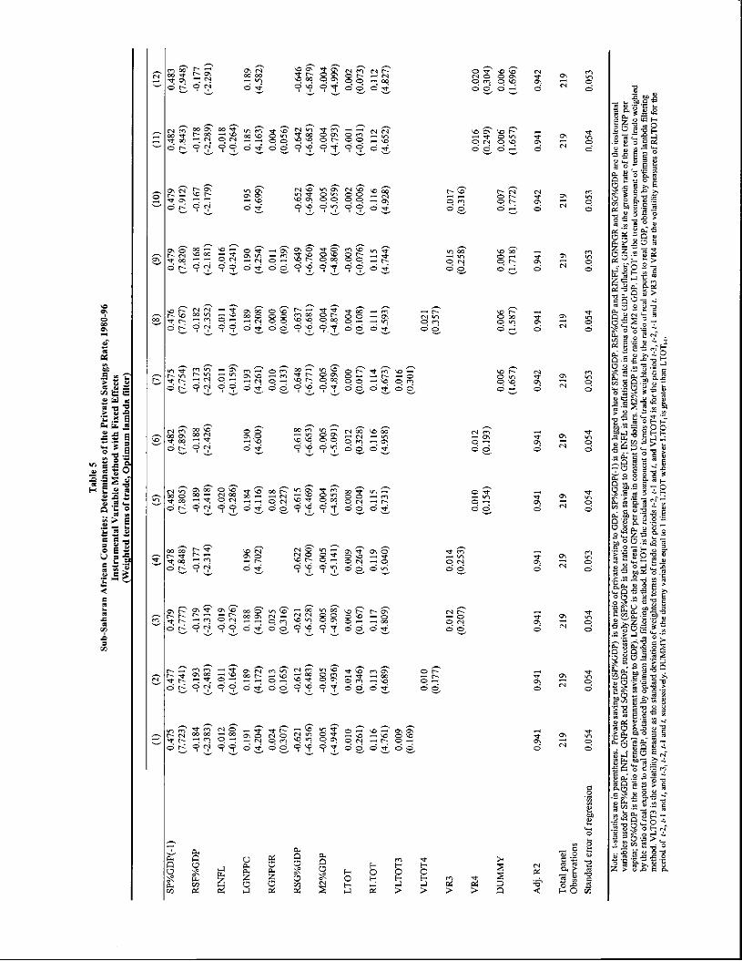
Tab
le 5
Su
b-Sa
hara
n A
fric
an C
ount
ries:
Det
erm
inan
ts o
f the
Priv
ate
Sav
ings
Rat
e, 1
980-
96
Inst
rum
enta
l V
aria
ble
Met
hod w
ith F
ixed
Effe
cts
(Wei
ghte
d te
rms of
trade
, O
ptim
um l
ambd
a fit
ter)
(1)
(2)
(3)
(4)
(5)
(6)
(7)
(8)
(9)
(10)
(11)
(12)
SP%GDP(-1)
0475
(7.723)
0.477
(7.741)
0.479
(7.777)
0.478
(7.848)
0.482
(7.805)
0.482
(7.893)
0.475
(7.754)
0476
(7
.767
) 0.
479
(7.8
20)
0.47
9 (7
.912
) 0,
482
(7.8
43)
0.48
3 (7
.948
) R
SF%
GD
P -0
.184
(-
2.38
3)
-0.1
93
(-2.
483)
-0
.179
(-
2,31
4)
-0.1
77
(-2,
314)
-0
.189
(-
2.41
8)
-0.1
88
(-2.
426)
-0
.173
(-
2.25
5)
-0.1
82
(-2.
352)
-0
.168
(-
2.18
1)
-0.1
67
(-2.
179)
-0
.178
(-
2.28
9)
-0.1
77
(-22
91)
RIN
FL
-0.0
12
(-0.
180)
-0
.011
(-
0.16
4)
-0.0
19
(-0.
276)
-0
.020
(-
0.28
6)
-0.0
11
(-0.
159)
-0
.011
(-
0.16
4)
-0,0
16
(-0.
241)
-0
018
(-0.
264)
L
GN
PPC
0.
19!
(4.2
04)
0.18
9 (4
.172
) 0.
188
(4.1
90)
0.19
6 (4
.702
) 0.
184
(4.1
16)
0.19
0 (4
.600
) 0.
193
(4.2
61)
0.18
9 (4
.208
) 0.
190
(4.2
54)
0.19
5 (4
.699
) 0.
185
(4.1
63)
0.18
9 (4
.582
) R
GN
PGR
0.
024
(0.3
07)
0.01
3 (0
.165
) 0.
025
(0,3
16)
0.01
8 (0
.227
) 0.
010
(0.1
33)
0.00
0 (0
.006
) 0.
011
(0.I
39)
0.00
4 (0
.056
) R
SG%
GD
P -0
.621
(-
6.55
6)
-0.6
12
(-6.
483)
-0
.621
(-
6.52
8)
-0.6
22
(-6.
700)
-0
,615
(-
6.46
9)
-0.6
18
(-6.
653)
-0
.648
(-
6.77
1)
-0.6
37
(-6.
681)
-0
.649
(-
6.76
0)
-0.6
52
(-6.
946)
-0
.642
(-
6.68
5)
-0.6
46
(-6.
879)
M
2%G
DP
-0,0
05
(-4.
944)
-0
.005
(-
4.93
6)
-0.0
05
(-4.
908)
-0
.005
(-
5.14
1)
-0.0
04
(-4.
853)
-0
.005
(-
5.09
!)
-0.0
05
(-4.
896)
-0
.004
(-
4.87
4)
-0.0
04
(-4.
860)
-0
.005
(-
5,05
9)
-0.0
04
(-4.
793)
-0
.004
(-
4.99
9)
LT
OT
0,
010
(0.2
61)
0.01
4 (0
.346
) 0.
006
(0.1
67)
0,00
9 (0
.264
) 0.
008
(0.2
04)
0,01
2 (0
.328
) 0.
000
(0.0
17)
0.00
4 (0
.108
) -0
.003
(-
0,07
6)
-0.0
02
(-0.
006)
-0
.001
(-
0.03
1)
0.00
2 (0
.073
) R
LT
OT
0,
116
(4.7
61)
0,11
3 (4
.689
) 0,
117
(4.8
09)
0,11
9 (5
.040
) 0.
115
(4.7
31)
0.11
6 (4
.958
) 0.
114
(4.6
73)
0.11
1 (4
.593
) 0.
115
(4.7
44)
0.11
6 (4
.928
) 0.
112
(4.6
52)
0.11
2 (4
.827
) V
LT
OT
3 0.
009
(0.1
69)
0.0 1
6 (0
.30!
) V
LT
OT
4 0.
0 10
(0.1
77)
0.02
1 (0
.357
) V
R3
0.01
2 (0
.207
) 0.
014
(0.2
53)
0.01
5 (0
.258
) 0.
017
(0.3
16)
VR
4 0.
010
(0.1
54)
0.01
2 (0
.193
) 0.
016
(0.2
49)
0.02
0 (0
.304
) D
UM
MY
0.
006
(1.6
57)
0,00
6 (1
.587
) 0.
006
(1,7
18)
0.00
7 (1
.772
) 0.
006
(1.6
57)
0.00
6 (1
.696
)
Adj
. R2
0.94
1 0.
941
0.94
1 0.
941
0.94
1 0.
941
0,94
2 0.
941
0.94
1 0.
942
0.94
1 0.
942
Tot
alpa
nel
219
219
219
219
219
219
219
219
219
219
219
219
Obs
erva
tions
Stan
dard
err
or o
f reg
ress
ion
0.05
4 0.
054
0.05
4 0.
053
0.05
4 0.
054
0.05
3 0.
054
0.05
3 0.
053
0,05
4 0.
053
RSF
%G
DP
and
RIN
FL, R
GN
PGR
and
RSG
%G
DP
are
the
inst
rum
enta
l N
ote:
t-s
tatis
lics
are
in p
aren
thes
es.
Priv
ate
savi
ng ra
te (S
l'°/Q
DP
) is
the
rat
io o
f pri
vate
savi
ng to
GD
P. S
P%G
DP(
- I) i
s th
e la
gged
val
ue o
f SP%
GD
P.
vari
able
s us
ed f
orSF
%G
DP,
IN
FL, O
NPU
Ran
d SG
%G
DP,
suc
eess
ivel
y(SF
%G
DP
isth
erat
io o
ffor
eign
savi
ngs
to G
DP;
IN
FL i
sthe
infl
atio
nrat
e int
erns
a of
the
GD
P de
flat
or;
GN
PGR
is [h
e gr
owth
rat
e of
ther
eal G
NPp
er
capi
ta; S
G%
GD
P is
the
ratio
of g
ener
al g
over
nmen
t sav
ing
to G
DP)
. LG
NPP
C i
s th
e lo
g of
real
GN
P pe
r cap
ita i
n co
nsta
nt U
S do
llars
. M
2%G
DP
is t
he ra
tio o
f M2
to G
OP.
LT
O'l'
is
the
tren
d co
mpo
nent
of
term
s of
trade
wei
ghte
d by
the
ratio
ofr
eal e
xpor
ts t
o re
al G
OP,
obt
aine
d by
opt
imum
lam
bda
filte
ring
met
hod.
RL
TO
T i
s th
e re
aidu
al c
ompo
nent
of
tenn
a of
trad
e w
eigh
ted
by th
e ra
tio o
f rea
l exp
orts
to
real
GO
P, o
btai
ned
by o
ptim
um la
mbd
a fi
lteri
ng
met
hod.
VL
TO
T3
isth
evol
atili
tym
easu
re as
the
stan
dard
devi
atin
n of
wei
ghte
dtem
,s of
trad
e fnr
peri
ods z
-2, i
-I a
nd!,
and
VL
TO
T4
is fo
rthe
peri
od :-
3, 1
-2,
I-I
ande
, V
R3
and
VR
4are
the
vol
atili
tym
easu
res
of R
LT
OT
fort
he
peri
odof
1-2
, I-I
and
I, a
nd 5
-3, 1
-2, 1
-I a
nd!,
suc
cess
ivel
y. D
UM
MY
is t
he d
umm
yvar
iabl
e eq
ual t
o I
times
LT
OT
whe
neve
rLl'O
T,is
grea
tert
han L
TO
T.5
.

-L-1101-j uo 1
o4o41 S
!Jflfl IOA
OU
24M Jfl sO
mu
04 imbo O
qoun Auiw
np oqi Si }vJ41JJ -ApA
issioons 7 PUS j-I '-l (-7 PU
B 'I pus i-i -s Jo pouad
oqlJoJLoL
paJo SO
JEIB
Um
U A
p1I4S1OA
045 PN
AP"0 (M
A ;pu -i '-J'(-;popodoqiJoJ
('IOL
lA pue
UB
I-i 'z-; spopadaoj aps1Jo UU
1 0l4MJ0 U
0qB!A
Op pJB
puBhsoL
fl SB alnsooulM
iuleoAoqs Si O
I-1A poqiim
2uuojij ouiom
iusd-uou £q pouioiqo 'juo W0J l spodxo IB
OJJ0 0401 041 A
q p0142mM
Open
JO SW
IO1 JO
iuouodmo, ienpsa O
qI Si JOIN
p04)0W 8uu01j!J oulouium
d-uou Aq pO
USB
lq0 dU
O 180.101
SIIOdX
D
BO
IJ0 0(150 011 X4
p0148iaMapu1oJo SU
LIO
1 Joluouodw
oopuol4 4li LO
JJ1 dUO 05 }JJ0O
51SJ 041 ! dUO
%t1'
0"-II°P 211 lur-ISLIO
n UI gjido,iod
jS0jjOiO
01415! DddN
Ol (duo 012U
!AB
S 1U0W
u10A08 elouo2Jo 01150014 i duO
%O
s gpdoo iod dN
O S
aloqIjO 1 44M
O1 091 S')(fldt4O
JO
ISIJO
p dUO
041J0 SLIUO)UI 0421 U
Oi)I3IJU
! 0541 0qJfl dU
O 0] S8U
IASS U
i!OJO
JJO 011v04 ! dU
O%
dS)X!0A
!SS000nS 'dU
O%
OS
PUS
MO
JNO
1dM
dUD
%1S'°J pO
ST] SoqousA
____________
541 dU
O"/0O
SU UB M
OdN
OM
_idNT
h PUTT dU
O%
dSM dU
O%
dSJ° OflirA
5)0220 41 ! (-)duo%ds ST
UD
0) 2u!A
BS oiotudjo 0!tflI 044 Si (auov5as) 0401 2u1tes O
WA
PST
oosaq100rndu! 0.10 soi1siwlw
-l :olof.
ccoo noo
pcoo tcoo
noo t'coo
vco'o no-c
not uoissoi2ojo 10110 p10p11015
suoqg,uosqçJ 611
6!?
61?
6TZ
61?
61?
61?
61?
61?
6!?
61?
61?
ausd 5101
Zt'60
160 lt'60
H'60
tt'6'0 1P6t
1f'60 060
lt'6'0 O
60 0t'60
spajj pax!j 14UM
PO
IIPIA
J OqtJt IS]IIO
IIIIIJISUI
96-0861 'alB! suiA
E5 flB
A!JJ alfljo s)ucuuualaq :sapjuno3 ucoajy uE
flqo5-qn5 9 aqcf
Ot-60
vu
(810-) 0f'o.o-
ot,0.o-
(1L9l)
(9191) (E
19i) (cL
cl) (ssc1)
(vuT)
coot coo-U
cooo
P00U
P00-U
cooo (8L1o-)
(t'Lco-) (occo-)
(too-) 0000-
(LOG
O)
0000 ((910-) !lO
0 (6010-) L
OO
t-
8t70-0-
(6cvo) 9100
(81cc) (L
ccc) (61st)
(o9c) (occc)
VIT
O
110 6110
9110 (H
O
91'OO
-
(voc-) coo-c-
(stc9-) 6190 (cvvo) 1(00
(19 co) 1100
(oco) (cco)
8100 8100
(ct9E)
(vosc) (69cc)
(lot) (oL
9c) (99cE
) (t'occ)
8110 L
110 P110
1110 8(10
@110
OttO
(p9cc)
(9oPo) (czvo)
(osro) (69(0)
(trio) (L
Vco)
(Ec@
o) (L
o@o)
(szco) (srvo)
(ocro) 1900
1900 scot
scot 900
6c0U
1900 (900
scoo 6coo
1900 0900
(cocc-) (L
zvc-) (arc-)
(tcic-) (oozc-)
(6Lcc-)
(cicc-) (G
EIc-)
(c9oc-) (990-c-)
coca- cooo-
cooo- coot-
coot- cooo-
coot- coot-
coot- cooo-
(8899-) (c!99-)
(1819-) (?Lv9-)
(o9c9-) (0819-)
(LLp9-) (9Ic9-)
(Ioc9-) (t9r9-)
Lt90-
6190- 1190
1190- 1E
90- £090-
96�0 t'090
1090- 6090
(taco) (L
sEo)
(9oco) 8(00
0(00 6(00
(66cc-) cooo-
(L9c9-)
0190 (cco) @
4'00
(8 LU
-U-)
coo 0-
(EL
cz-) (V
Pc-z-)
8610 8610-
(csL'L
) (oE
LL
) 9L1'O
8L
t'O
(c19P) (or't')
(L9cp)
(LLov) (900f)
(PLoP)
(ccct') (PL
o-f) (cocP)
(9?ot) (6c6E
) (9sot)
1610 9810
610 (810
1810 9810
0610 (810
6810 1810
0810 1810
AY
il411U
flIA
(MA
l'tOflA
£IOJT
IA
LO
L'T
U
tori
dUO
%Z
}N
dQO
%D
SM
MD
dMO
M
DddN
Oq
'MN
IM
dUD
%1JSM
(6c9o) (((c-a)
(8c90) ocoo
ovoo Icoo
(pojo-) (czIo)
(Lno) (oio)
(oLoo) (9T
ro) 9000-
8000 6000
9000 cooc
1100 (coc-z-)
(oLd-)
(Lzcz-)
(it'vz-) (v9c1-)
(dc-?-) (L8E
z-) (o(cz-)
(661?-) t-810-
P810- L
610- 6810-
6610- L
61O-
@810-
1810- coo-
(paL) (889L)
(8c9L) (L19L)
(6c8L) (I'E
8L) (01st)
(l6LL) (Z
PLL)
(aLL) E
LPO
9LV
0 ?LP
0 ILV
O
1810 9810
6L10 £810
6L10 6L10
(soco) 0100
(to 9810-
(tO
U 0
(01) (6)
(s) (L
) (9)
(c) (v)
(c) (1)
(1)
(nu 3!a!amcacd-uoN
'apc13 JO
smiaj pa)qM
aJ
(1-)duo%ds
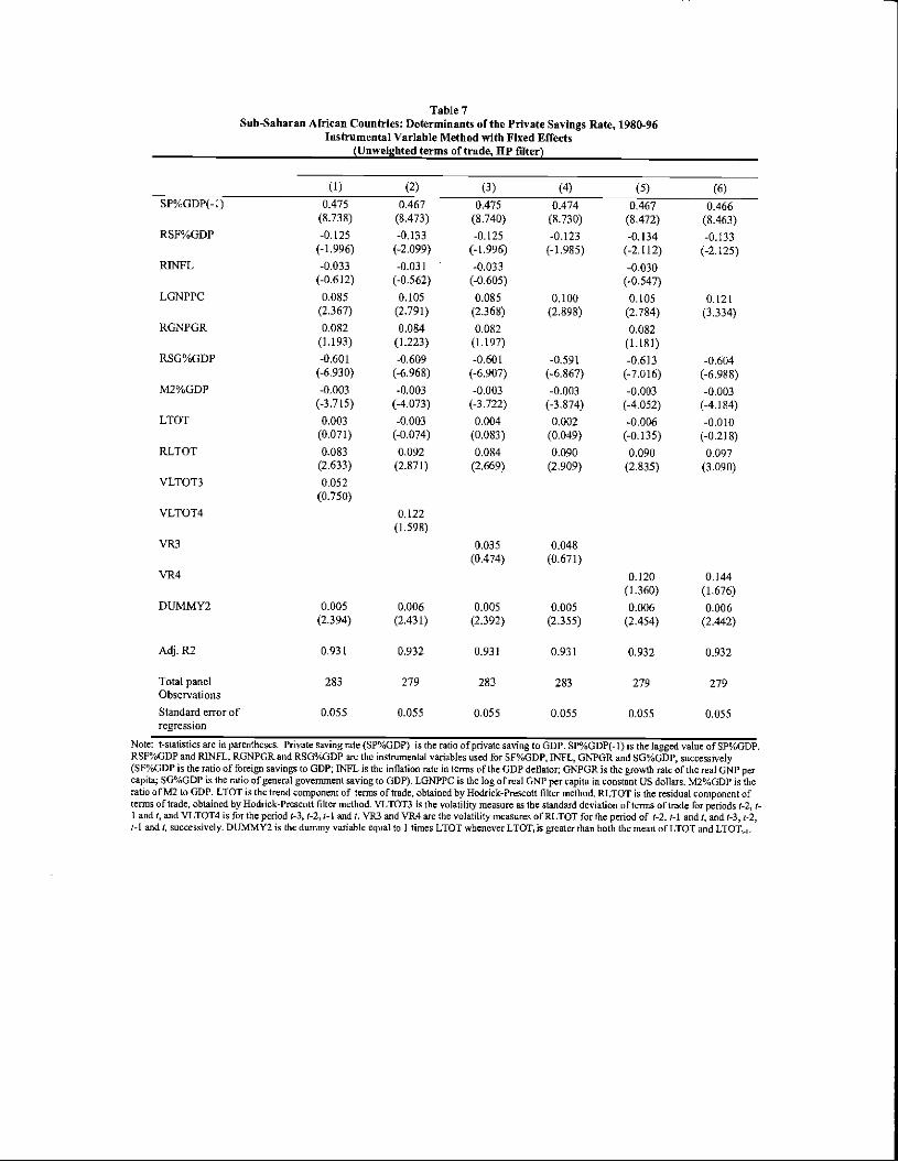
Table 7Sub-Saharan African Countries: Determinants of the Private Savings Rate, 1980-96
Instrumental Variable Method with Fixed Effects(Unweighted terms of trade, lIP filter)
(1) (2) (3) (4) (5) (6)SP%GDP(-l) 0.475 0.467 0.475 0.474 0467 0.466
(8.738) (8.473) (8.740) (8.730) (8.472) (8.463)RSF%GDP -0.125
(-1.996)-0.133
(-2.099)-0.125
(-1.996)-0.123
(-1.985)-0.134
(-2.112)-0.133(-2.125)
RINFL -0.033
(-0.612)-0.031
(-0.562)-0.033(-0.605)
-0.030(-0.547)
LGNPPC 0,085(2.367)
0.105
(2.791)0.085
(2.368)0.100
(2.898)0.105
(2.784)0.i21
(3.334)RGNPGR 0.082
(1.193)0.084
(1.223)0.082
(1.197)0.082
(1.181)RSG%GDP -0.601
(-6.930)-0.609(-6.968)
-0.601(-6.907)
-0.591
(-6.867)-0.613
(-7.016)-0.604(-6.988)
M2%GDP -0.003(-3.715)
-0.003(-4.073)
-0.003(-3.722)
-0.003
(-3.874)-0.003
(-4.052)-0.003(-4.184)
LTOT 0.003(0.071)
-0.003(-0.074)
0.004(0.083)
0.002(0.049)
-0.006
(-0.135)-0.010
(-0.218)RLTOT 0.083
(2.633)0.092
(2.871)0.084
(2.669)0.090
(2.909)0.090
(2.835)0.097
(3.090)VLTOT3 0.052
(0.750)VLTOT4 0.122
(1.59 8)VR3 0.035
(0.474)0.048
(0.67 1)VR4 0.120
(1.360)0.144
(1.676)DUMMY2 0.005
(2.394)0.006
(2.431)0.005
(2.392)0.005
(2.355)0.006
(2.454)0.006
(2.442)
Adj. Ri 0.931 0.932 0.931 0.931 0.932 0.932
Totai panel 283 279 283 283 279 279Observations
Standard error of 0.055 0.055 0.055 0.055 0.055 0.055regression
Note: t-stalistics are in parentheses. Private saving rate (SP%GDP) is the ratio of private saving to GDP. SP%GDP(-1) is the lagged value ofSP%GDP.RSF%GDP and RINFL, RONPOR and RSG%GDP are the instrumentai variables used for S%CDP, INEL, GNPGR and SG%ODP, successively(SF%GDP is the ratio of foreign savings to GDP; INFL is the inflation rate in terms of the GDP deflator; GNP0R is the growth rate of the eeal CiNP percapita; SG%ODP ia the ratio ofgeneral government saving to ODP). LGNPPC is the log ofecal GNP per capita in constant US dollars, M2%ODP is theratio of M2 to GDP. LTOT is the trend component of terms of trade, obtained by Hodrick-Prescott filter method. RLTOT is the residual component oftcnns oftrade, obtained by l-lodsick-Prescott filter snethod. VLTOT3 ia the volatility measure as the standard deviation ofterms oftrade for periods t-2, I'-I ande, and VLTOT4 is for the period t-3, t-2, I-I andL VR3 and VR4 are the volatility measures ofRLTOT for the period of 1-2, i-i and I, and (-3, t-2,1-I and t, successively. DUMMY2 is the dunmay variable equal to I times LTOT whenever LTQTI is greater than both the mean ot'LTOT and LTOTw.

TableSSub-Saharan African Countries: Determinants of the Private Savings Rate, 1980-96
Instrumental Variable Method with Fixed Effects(Unweighted terms of trade, Optimum lambda filter)
(1) (2) (3) (4) (5) (6)
SP%GDP(-l) 0.518 0.515 0.518 0.520 ft516 0.517(8.537) (8.413) (8.546) (8.676) (8A08) (8.530)
RSF%GDP -0.110(-1.548)
-0.110
(-1.543)-0106
(-1.494)-0.097
(-1.386)-0.107
(-1.495)-0.098(-1.398)
RINEL -0.046(-0.719)
-0.045
(-0.695)-0.049(-0.762)
-0.047
(-0.730)LGNPPC 0.173
(3.673)0.175
(3.672)0.170
(3.641)0.182
(4.148)0.173
(3.640)0.186
(4.186)RGNPGR 0.029
(0.345)0.039
(0.468)0.024
(0.294)0.032
(0.400)RSG%GDP -0628
(-6.428)-0.619(-6.284)
-0.624(-6.407)
-0.630(-6.528)
-0.620
(-6.316)-0.625(-6.432)
M2%GDP -0.004(-4.428)
-0.004(-4.397)
-0.004(-4.445)
-0.004(-4.612)
-0.004
(-4.415)-0.004
(-4.595)LTOT -0.044
(-0.749)-0.044(-0.739)
-0.041(-0.700)
-0.039
(-0.677)-0.043
(-0.718)-0.041
(-0.718)RLTOT 0.108
(3.323)0.103
(3.192)0.115
(3.519)0.116
(3.762)0.107
(3.269)0.108
(3.496)VLTOT3 -0.027
(-0.33 8)VLTOT4 0.071
(0.799)VR3 -0.039
(-0.448)-0.031(-0.367)
VR4 0.069(0.673)
0.078(0,775)
DUMMY2 0.006(2.033)
0.005(1.776)
0.006
(2.085)0.007
(2.216)0.005
(1.790)0.006
(1.917)
Adj. It? 0.936 0.935 0.936 0.936 0.935 0.936
Total panel 224 224 224 224 224 224Observations
Standarderrorof 0.056 0.056 0.056 0.055 0.056 0.056regression
Note: t-statisties are in parentheses. Private saving rate (SP%GDP) is the ratio of private saving to GOP. SP%ODP(-1) is the lagged value ofSP%ODP.RSF%GDP and RINFL, RONFUR and RSG%GDP are the instrumental variables used for SF%GDP, INUL, GNPGR and SG%GDP, successively(SF%GDP is the ratio of foreign savings to ODP; INFL is the inflation rate in terms of the GDP deflator; ONPGR is the grotth rate of the real C}NP percapita; SG%GDP is the ratio ofgeneral government saving to GDP). LGNPPC is the log of real GNP per capita in constant US dollars. M2%GDP is theratio ofM2 to ODE LTOT is the tread component of terms oflrade, obtained by optimum lambda filtering method. RLTOT is the residual component ofterms of trade, obtained by optimum lambda filtering method. VLTOT3 is the volatility measure as the standard deviation of temss of trade for periods2, i-i and and VLTOT4 is for the period 1-3, !-2,t- I and 1, VR3 and VR4 are the volatility measures of RLTOT for the period of t-2, s-I and I, and t-3,(-2, 1-1 and , successively. DUMMY2 it the dummy variable equal to I times LTOT whenever LTOT, is greater than both The mean of LTOT andLTOT,1.

Table 9Sub-Saharan African Countries: Determinants of the Private Savings Rate, 1980-96
Instrumental Variable Method with Fixed Effects(Unweighted terms of trade, Non-parametric filter)
(1) (2) (3) (4) (5) (6)
SP%GDP(- I)
RSF%GDP
RINFL
LGNPPC
RGNPGR
RSG%GDP
M2%GDP
LTOT
RLTOT
VLTOT3
VLTOT4
VR3
VR4
DUMMY2
AdJ. 1(2
Total panelObservations
Standard error ofregression
0.505 0.502 0.504 0.506 0.503 0.505(8.051) (7.949) (8.041) (8.221) (7.988) (8.143)-0.128 -0.126 -0.126 -0.116 -0.124 -0.115(-1.801) (-1.778) (-1.763) (-1.669) (-1.734) (-1.652)-0.042 -0.040 -0.045 -0.042
(-0,677) (-0.641) (-0724) (-0.670)0.144 0.150 0.142 0.153 0.146 0.158
(3.336) (3.430) (3.318) (3.806) (3.379) (3.911)0.041 0.048 0.035 0.042
(0.505) (0.593) (0.442) (0.528)-0.642 -0.634 -0.638 -0.645 -0.636 -0.642
(-6.473) (-6.335) (-6.456) (-6.598) (-6.411) (-6.540)-0.004 -0.004 -0.004 -0.004 -0.004 -0.004
(-4.665) (-4.646) (-4.716) (-4.900) (-4.672) (-4.861)-0.020 -0.023 -0.017 -0.020 -0.020 -0.024
(-0.401) (-0.453) (-0.331) (-0.392) (-0.395) (-0.471)0.107 0.104 0.115 0.121 0.109 0.115
(2.846) (2.769) (3.024) (3.303) (2.863) (3.137)-0.003
(-0.042)0.082
(0,93 7)
-0.014(-0.181)
-0.005
(-0.072)0.067
(0.705)0.080
(0.859)0.005 0.005 0.005 0.005 0.005 0.005
(1.972) (1.886) (1.964) (1.959) (1.918) (1.917)
0.936 0.935 0,936 0.936
224 224 224
0.935
0.056 0.056 0.056
0.93 6
224 224 224
0.05 5 0.056 0.056
Note: t-statisties are in parentheses. Private saving rate (SP%GDl') is the ratio of private saving to GD?. SP'/aGDP(-l) is the lagged value of SP%GDP.RSI1%GDP and RINFL, RGNPGR and ItSG%tl0P are the instrumental variables used for SF'/SGDP, INFL, GNPGR and SG%GDP, soecessively(SF%GDP is the ratio of foreigti savings to GDP; INFL is the inflation rate in terms of the GD? deflator; GNPGR is the growth rate of the real GNP percapila; SG%GDP is the ratio ofgeneral government saving to GD?). LGNIPPC is the log ofreal GNP per capita in constant US dollars. M2%GDt' is theratio of M2 to GDP. LTOT is the trend component of tenna of trade, obtained by non-parametric filtering method, RLTOT is the residual component oftcnna oftrade, obtained by non-parametric filtering method. VLTOT3 is the volatility measure as the standard deviation of terms of trade for periods /-2,I-I and C, and VLTOT4 is for the period 1.3, t-2, /-landt. VR3 and VR4 are the volatility measures of RI.TOT for the period of 1-2, 1-1 and /. and 1-3, t-2,I-I and', successively. Dl,fl\tM'Y2 is the dummy variable equal to 1 times LIOT whenever LTOrI is greater than both the mean ofLTOT and LTOT,.,.

Table 10Sub-Saharan African Countries: Determinants of the Private Savings Rate, 1980-96
Instrumental Variable Method with Fixed Effects
(1) (2) (3) (4) (5) (6)
SP%GDP(-1) 0.460 0.454 0.459 0.456 0.454 0.452(8.675) (8.434) (8.627) (8.577) (8.363) (8.324)
RSF%GDP -0.111
(-1.802)-0.116
(-1.861)-0.111
(-1.808)-0.113(-1.847)
-0.115(-L841)
-0.118
(-1.908)RINFL -0.010
(-0.176)-0.006
(-0.108)-0.015
(-0265)-0.010
(-0.179)LGNPPC 0.090
(2.644)0.095
(2.725)0.088
(2.574)0.102
(3.159)0.094
(2.693)0.109
(3.275)RGNPGR 0.088
(1.291)0098
(].431)0.090
(1.316)0.101
(1.469)RSG%GDP -0.595
(-7.060)-0.602
(-7.061)-0.595
(-7.034)-0.579
(-6.999)-0.60!
(-7.049)-0.584(-6.999)
M2%GDP -0.003
(-3.850)-0.003
(-4.093)-0.003(-3.799)
-0.003
(-3.949)-0.003
(-4.065)-0.003(-4.179)
LTOT -0.009(-0.261)
-0.002
(-0.063)-0.009(-0.251)
-0.009(-0.263)
-0.003
(-0.088)-0.005(-0.144)
RLTOT 0.110(4,511)
0.107(4.373)
0.108(4.401)
0.112(4.745)
0.106(4.303)
0.112(4.706)
VLTOT3 0,065(1.294)
VLTOT4 0.082(1.50 1)
VR3 0.100(1.711)
0.099(1.820)
VR4 0.115(1.657)
0.111
(1.665)DUMMY2 0.006
(2.127)0.006
(2.110)0.006
(2.111)0.006
(2.008)0.006
(2.101)0.006
(1.986)
Adj. R2 0.934 0.934 0,934 0.934 0.934 0.934
Total panel 283 279 283 283 279 279Observations
Standard error of 0.054 0.054 0.054 0.054 0.054 0.054regression
Note; s-statistics are in parentheses. Private saving rate (SP%60P) is the ratio ofprivate saving to GOP. SP%SJDP(-l) is the lagged value ofSP%GDP.RSF%GDP and RINEL, RGNPGR and RSG%GDP are the instrumental variables used for SF%GDP, INFL, GNPGR and SG%GDP, successively(SF%GDP is the ratio of foreign savings to GOP; INFL is the inflation rate in tersais ofthe GDP deflator; GNPGR is the growth rate ofthe real GNP percapita; SG%GDP is the ratio ofgeneral government saving to GOP). LGNPPC is Ihe log of real GNP per capita in constant US dollars. M2%GDP is theratio of M2 10 GDP. LTOT is the trend component of terms of trade weighted by the ratio of real exports to real GOP, obtained byHodrick-Prescott fillermethod. RLTOT is lhe residual component of Irons ofirade weighted by lhe ratio of real exports to real GDP, obtained by Uodrick-Preacott filtermethod. VLTOT3 ia the volatility measure as Ihe standard deviation of weighted tenns oftrade for the periods of 1-2, f-I and t, and VLTOT4 is for theperiod t-3, 1-2, f-I and 1. VR3 and VR4 are the volatility measures of RLTOT fortheperiod of h2, 1-1 and, and /-3, s-2, f-I and f. successively.DIJMMY2 is the dummy variable equal tot times LTOT wheaeevcrLToT,ia greater than both the mean of LTOT and LTOT,.1.
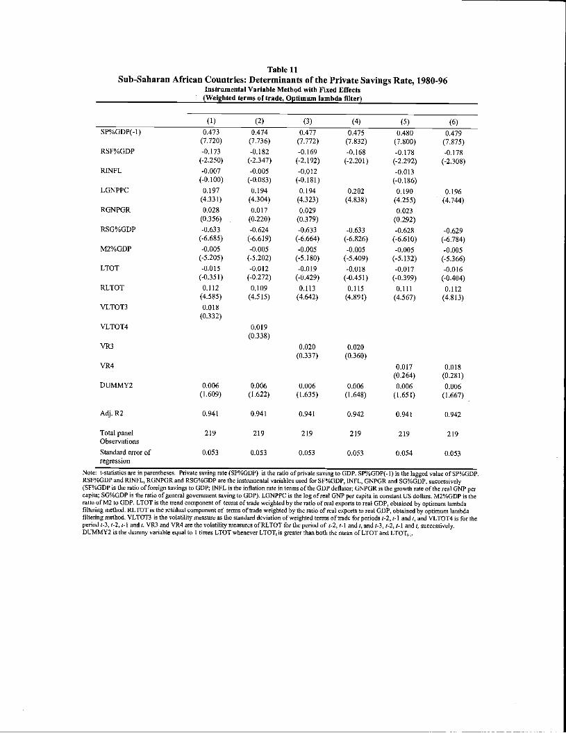
Table 11Sub-Saharan African Countries: Determinants of the Private Savings Rate, 1980-96
Instrumental Variable Method with Fixed Effects(Weighted terms of trade, Optimum lambda fitter)
(1) (2) (3) (4) (5) (6)
SP%GDP(-1) 0.473 0.474 0.477 0.475 0.480 0.479(7.720) (7.736) (7.772) (7.832) (7.800) (7.875)
RSF%GDP -0.173
(-2.250)
-0.182
(-2.347)
-0.169
(-2.192)
-0.168
(-2.201)
-0.178
(-2.292)
-0.178
(-2.308)
RINFL -0.007
(-0.100)
-0.005
(-0.083)
-0,012
(-0.181)
-0.013
(-0.186)
LUNPFC 0.197
(4.331)
0.194
(4.304)
0.194
(4.323)
0.202
(4.838)
0.t90
(4.255)
0.196
(4.744)
RGNPGR 0.028
(0.356)
0.017
(0.220)
0.029
(0.379)
0.023
(0.292)
RSG%GDP -0.633
(.6.685)
-0.624
(-6.619)
-0.633
(-6.664)
-0.633
(-6.826)
-0.628
(-6.610)
-0.629
(-6.784)
M2%GDP -0.005
(-5.205)
-0,005
(-5.202)
-0.005
(-5.180)
-0.005
(-5.409)
-0.005
(-5.132)
-0.005
(-5.366)
LTOT -0.015
(-0.35 I)-0.012
(-0.272)
-0.019
(-0.429)
-0.018
(-0.451)
-0.017
(-0.399)
-0.016
(-0.404)
RLTOT 0.112
(4.585)
0,109
(4.515)
0.113
(4.642)
0.115
(4.891)
0.111
(4.567)
0.112
(4.813)
VLTOT3 0.018
(0.332)
VLTOT4 0.0 19
(0.33 8)
VR3 0.020
(0.337)
0.020
(0.360)
VR4 0.017
(0.264)
0.018
(0.281)
DUMMY2 0.006
(1.609)
0.006
(1.622)
0.006
(1.635)
0.006
(1.648)
0.006
(1.651)
0.006
(1.667)
Adj. P.2 0.941 0.94 1 0.941 0.942 0.941 0.942
Total panel 219 219 219 219 219 219Observations
Standard error of 0.053 0.053 0.053 0.053 0.054 0.053regression
Note: S-statistics are inparcntheses. Private savingrate (SP%GD?) is the ratio of private saving to GOP. SP%UDI'(-l) is the lagged value ofS?VsGDP.RSF%GD? and RINFL, RGNPGR and RSG%GDP are the instnsmental variablea used for SF%GDP, NFL, GNPGR and SG%GDP, successively(SF%GDP is the ratio of foreign savings to (JO?; NFL is the inflation rate in semis of the GD? deflator; GNPGR is the growth rate of the real UN? percapita; SG%GDP is she ratio ofgeocral government saving to 00?). LGNPPG is the log of reat UN? per capita in constant US dollars, M2%GD? is theratio ofM2 to GDP. LTOT is the trend component of terms ofirade weighted by tbe ratio ofreal exporta to real GD?, obtained by optimum lambdafilteriag method. RLTOT is the residual component of terms ofirade weighted by the ratio ofreal exports to real GD?, obtained by optimum lamhdafilteeiag method. VLTOT3 is the volatility measure as the standard deviation of weighted terms oftaadc for periods 1-2, t- I andi, and VLTOT4 is for theperiod 5-3, 5-2, 2.1 and I. fl3 and VR4 am the volatilitynieasures ofRLTOT for the period of 5-2, r-l andt, and t-3, 5-2, 2-1 and I, successively.DUMMY2 is the dummy variable equal to I times LTOT whenever LTOT,ia greater than both the mean of LTOT and LTOTI.I.

Total pane] 219Observations
Standard error of 0.054regression
0.054 0.054 0.054
219 219 219
Note: t-statistics are in parentheses. Private saving rate (SP%GDP) is the ratio ofprivale saving to GOP. SP%GDP(- I) is the lagged value ofSP%GDP.RSF%GDP and RINFL, RGNPGR and RSG%GDP areThe inatrurnental variables used for SF%GDP, INH, GNPGR and SG%GDP, suceessivety(SF%GOP is the ratio of foreign savings to GOP; JNFL is the inflation rate in tenns ofThe GOP deflatog GNPGR is The growth rate ofthe real GNP percapita; SG%GDP lathe ratio of general government saving to GDP). LGNPPC is the log of real GNP per capita in constant ff8 dollars. M2%GDP is theratio of M2 to GOP. LTOT is Ihe trend component of terms of trade weighted by the ratio of real exports to rent GOP, obtained bynon-parasoetriefiltering method. RLTOT is the residual component of terms oftrade weighted by the ratio of mat exports to mat GOP, obtained by non-parametricfiltering method. VLTOT3 ia the volatitity measure as the standard deviation ofweiglited lernts of trade for periods 1-2,1-I andt, and VLTOT4 is for theperiod I-], 1-2, f-I andt. VIR3 and VR4 are the volatility measures of RLTOT fortheperiod of (-2, t-t and:, and 1-3, t-2, f-I and'. successively.OLJI\iIMY2 is the dummy variable equal to t times LTOT whenever LTOT1 is greater than both the mean of LTOT arid LTOT,i.
Table 12Sub-Saharan African Countries: Determinants of the Private Savings Rate, 1980-96
Instrumental Variable Method with Fixed Effects(Weighted terms of trade. Non-parametric filter)
(I) (2) (3) (4) (5) (6)SP%GDP(-1)
RSF%ODP
RINFL
LGNPPC
RGNPGR
RSG%GDP
M2%GDP
LTOT
RLTOT
VLTOT3
VILTOT4
VR3
VR4
DUMMY2
Adj. R2
0.478 0.479 0.483 0.478 0.485 0.481(7.740) (7.750) (7.788) (7.799) (7.840) (7.858)-0.180 -0.190 -0,178 -0.179 -0.191 -0.193
(-2.320) (-2.429) (-2.276) (-2.322) (-2.445) (-2.496)0.019 0.020 0.003 0.005(0.295) (0.307) (0.052) (0.091)0.185 0.183 0.183 0.192 0.186 0.193
(4.049) (4.025) (4.056) (4.552) (4.133) (4.612)0.055 0.044 0.054 0.049(0.709) (0,564) (0.710) (0.642)-0.610 -0.602 -0.603 -0.595 -0.610 -0.603
(-6.374) (-6.3 13) (-6.308) (-6.408) (-6.377) (-6.486)-0.005 -0.005 -0.005 -0.005 -0.005 -0.005
(-5.221) (-5.221) (-5.254) (-5.418) (-5.348) (-5.518)0.049 0.051 0.049 0.049 0.052 0.051
(0.818) (0.888) (0.836) (0.902) (0.932) (1.003)0.115 0.110 0.114 0.118 o.J 10 0.114
(3.561) (3.419) (3.524) (3.773) (3.424) (3.669)0.018
(0.337)0.02 0
(0.3 53)
-0.000
(-0.006)
-0.004
(-0.062)
-0.045
(-0.541)-0.047(-0.565)
0.003 0.004 0.003 0.003 0.003 0.003(1.240) (1.252) (1.080) (1.046) (1.227) (1.201)
0.940 0.940
219
0.940 0.941 0.941 0.941
219
0.054 0.054