savitribai phule pune university - mathskthm.me.pnmathskthm.me.pn/multivariable calculus.pdf ·...
TRANSCRIPT

Savitribai Phule Pune University
A Text Book for S.Y.B.Sc./S.Y.B.A. Mathematics (2013 Pattern)
PAPER II(A)-MT 222(A)
MULTIVARIABLE CALCULUS
Panel of Authors
S.S. Munot (Convenor)Dr.S.B.Gaikwad
S.A.Ghule
Editors
Dr.P.M. Avhad Dr.S.A.Katre
Conceptualized by Board of Studies (BOS) in Mathematics, Savitribai Phule Pune University, Pune.
i
Page ii
Preface
This text book is an initiative by the BOS Mathematics, Savitribai Phule Pune University. The
syllabus of Savitribai Phule Pune University is always considered commendable, with a list of re-
puted books in the subject recommended for reference. Many times teachers face difficulty in doing
justice to every aspect covered collectively by all these books. So, while preparing new syllabus for
S.Y.B.Sc./S.Y.B.A. it was thought the University should prepare textbooks for Mathematics with
the following objectives:
1. Uniformising notations, definitions and to focus on important aspects of revised syllabus which
need to be stressed and understood.
2. Collecting all relevant topics, problems, questions prescribed in syllabus.
3. Providing a ready reference to teachers and students.
The book is written in accordance with the new prescribed syllabus of S.Y.B.Sc., S.Y.B.A. Mathe-
matics (2013 Pattern), for the Paper II(A)- MT 222(A): Multivariable Calculus II (Second Term).
The syllabus deals with important topics in Mathematics, Vector Calculus.
This book consists of a detail introduction at the beginning of each chapter, several illustrative
examples and problems for practice with hints and solutions given at the end of each section. A
proper understanding of all the illustrative examples would go a long way in making the subject fully
comprehensible.
In case of queries/suggestions, send an email to: sumati.munot @ gmail.com
We hope our endeavor will benefit both students and teachers.
-Authors
ii

Page iii
Acknowledgment
We sincerely thank the following University authorities for their constant motivation, guidance
and valuable help in the preparation of this book.
• Dr. W. N. Gade, Hon. Vice Chancellor, Savitribai Phule Pune University, Pune.
• Dr. V. B. Gaikwad, Director BCUD, Savitribai Phule Pune University, Pune.
• Dr. K. C. Mohite, Dean, Faculty of Science, Savitribai Phule Pune University, Pune.
• Dr. B. N. Waphare, Professor, Department of Mathematics, Savitribai Phule Pune Univer-
sity, Pune.
• Dr. M. M. Shikare, Professor, Department of Mathematics, Savitribai Phule Pune University,
Pune.
• Dr. V. S. Kharat, Professor, Department of Mathematics, Savitribai Phule Pune University,
Pune.
• Dr. V. V. Joshi, Professor, Department of Mathematics, Savitribai Phule Pune University,
Pune.
• Mr. Dattatraya Kute, Senate Member, Savitribai Phule Pune University; Manager, Savit-
ribai Phule Pune University Press.
• All the staff of Savitribai Phule Pune University press.
iii

Page iv
Syllabus: Paper II(A) MT 222(A):Multivariable Calculus
(1) Vector Valued Functions: . . . [14]
1.1 Vector valued function .
1.2 Limit and continuity of vector function .
1.3 Derivative of vector function and motion .
1.4 Differentiations rules.
1.5 Constant vector function and its necessary and sufficient condition .
1.6 Integration of vector function of a scalar variable .
1.6 Arc length and unit tangent vector T .Curvature and unit normal vector N.
(2) Line Integrals: . . . [16]
2.1 Definition and evaluation of line integral.
2.2 Properties of line integrals .
2.3 Vector fields,work,circulation and flux across smooth curves.
2.4 Path independence,potential function,conservative field.
2.5 Green’s theorem in plane,evaluating integrals using Green’s theorem.
(3) Surface and Volume Integrals: . . . [18]
3.1 Surface area and surface integrals.
3.2 Surface integral for parametrized surfaces.
3.3 Stokes theorem(without proof).
3.4 The Gauss divergence theorem(proof for special regions).
Text book: Prepared by the BOS Mathematics, Savitribai Phule Pune University, Pune.
Recommended Book: Thomas’ Calculus’ 11th Edition, G.B. Thomas. Revised by Maurice D.
Weir, Joel Hass and Frank R. Giordano. Pearson Education 2012. Articles: 13.1, 13.3, 13.4, 16.1 to
16.8.
Reference Books:
(1) Basic Multivariable Calculus, J.E. Marsden, A.J. Tromba, A. Weinstein. Springer Verlag
(Indian Edition).
(2) A textbook Vector Calculus, Shanti Narayan, R.K. Mittal. S. Chand and Company.
(3) Advanced Calculus, John M., H. Olmsted. Eurasia Publishing House, New Delhi (1970).
(4) Calculus Vol.2 (2 nd Edition), T.M. Apostol. John Wiley, Newyork (1976).
iv

Contents
Chapter 1. Vector Valued Functions 1
1. Vector Valued Functions: 1
2. Limit and Continuity of Vector Function 2
3. Derivative of Vector Function and Motion 7
4. Differentiation Rules 9
5. Constant Vector Function 11
6. Integration of Vector Function 14
7. Arc Length 15
8. Exercise 20
9. Answers 21
Chapter 2. Line Integrals 23
1. Definition and Evaluation of Line Integral 23
2. Mass and Moment 26
3. Work,Circulation and Flux 30
4. Path Independence,Potential Functions 34
5. Green’s Theorem in Plane 40
6. Illustrative Examples 45
7. Exercise 56
8. Answers 59
Chapter 3. Surface and Volume Integrals 61
1. Surface Area and Surface integrals 61
2. Surface Integral for parametrized surface 70
3. Stokes’s Theorem 76
4. The Divergence Theorem 79
5. Exercise 88
6. Answers 90
v

CHAPTER 1
Vector Valued Functions
Introduction: In this chapter we shall introduce the concepts of vector valued functions of a
single scalar variable and those of their limits, continuity and derivability. In addition to these the
notion of Indefinite Integral of a vector valued functions of a single variable will be introduced.
In this chapter we use similar results from scalar valued functions to prove the corresponding number
of theorems in vector calculus.
1. Vector Valued Functions:
Consider a particle or an object P moves in space; let us consider the motion in some time interval
say I = [a, b] let r denote the displacement of a particle P from fixed point O to P at time t. Let W
be the set of all values assumed by r as t assumes from a to b.
The relation {(t, r)|t ∈ I} defines a function from I to W. We write r = r(t), t ∈ I. Here r is a vector
of a scalar variable t
If the coordinates of particle defined on I as x = f(t), y = g(t), z = h(t), t ∈ I. The point
(x, y, z) = (f(t), g(t), h(t)) describes curve in space that we call the particles path.
A curve in space in vector form can be represented by
r(t) = OP = f(t)i+ g(t)j + h(t)k . . . (1)
1

Limit and Continuity of Vector Function Page 2 Vector Valued Functions
from the origin to the particles position P (f(t), g(t), h(t)) at time t.
The scalar functions f, g, h are the components of r(t).
Equation (1) gives r as a vector function of the real variable t on I.
Definition 1.1. (Vector valued function): Let A be a non-empty subset of set of real numbers
R and W be a non-empty subset of R3.
A vector function or vector valued function r on a domain set A is a rule that assigns a unique vector
in space W to each element in A.
We write it as r = r(t).
A vector function r, can be expressed interms of its components as
r(t) = f(t)i+ g(t)j + h(t)k.
Examples :
1. If r = r(t) is a position vector or displacement of a particle from origin to a point P at a
time t, then r is a vector function of a scalar variable t.
The velocity and acceleration of a moving particle are also vector function of a scalar variable
t.
2. r = a cos ti+ b sin tj + ok and r = at2i+ 2atj + ok are the vector equations of an ellipse and
a parabola resp.
3. r = (t2 + t)i+ 5t3j + 3tk defines any curve where t is a parameter.
2. Limit and Continuity of Vector Function
We define limit of a vector function,similar to as we define limit of a scalar function.
Definition 1.2. (Limit of a function): Let f = f(t) be a vector function of a scalar variable
t, defined on a domain A and L a constant vector function.If for given each ε > 0, there is a scalar
δ > 0, such that whenever 0 < |t− t0| < δ, we have |f(t)− L| < ε, then we say that f(t) tends to the
limit L as t tends to t0 and we write limt→t0
f(t) = L. We read this as the limit as t→ t0 of f(t) is L.
Theorem 1.1. Let f(t) = f1(t)i + f2(t)j + f3(t)k be a vector function of a scalar variable t and
L = l1i+ l2j + l3k be a constant vector function.
Then limt→t0
f(t) = L if and only if limt→t0
f1(t) = l1, limt→t0
f2(t) = l2 and limt→t0
f3(t) = l3.
Proof. Suppose limt→t0
f(t) = L. By the definition of limit, for a given ε > 0 there is a δ > 0 such
that whenever 0 < |t− t0| < δ, we have |f(t)− L| < ε . . . (1)
2

Vector Valued Functions Page 3 Limit and Continuity of Vector Function
We have
|f(t)− L| = |(f1(t)i+ f2(t)j + f3(t)k)− (l1i+ l2j + l3k)|
= |(f1(t)− l1)i+ (f2(t)− l2)j + (f3(t)− l3)k|
From this equation we get, |f1(t)− l1| ≤ |f(t)− L| < ε, |f2(t)− l2| < ε and |f3(t)− l3| < ε, whenever
0 < |t− t0| < δ
∴ limt→t0
f1(t) = l1, limt→t0
f2(t) = l2, limt→t0
f3(t) = l3.
Thus if limt→t0
f(t) = L then limt→t0
f1(t) = l1, limt→t0
f2(t) = l2 and limt→t0
f3(t) = l3.
Conversely, suppose limt→t0
f1(t) = l1, limt→t0
f2(t) = l2 and limt→t0
f3(t) = l3.
For any ε > 0, there exist positive numbers δ1, δ2 and δ3 such that
|f1(t) = l1| <ε
3, when 0 < |t− t0| < δ1
|f2(t) = l2| <ε
3, when 0 < |t− t0| < δ2
|f3(t) = l2| <ε
3, when 0 < |t− t0| < δ3
Take δ = min{δ1, δ2, δ3}. Then above three inequalities hold for 0 < |t− t0| < δ.
Thus for 0 < |t− t0| < δ, we have
|f(t)− L| =|(f1(t)− l1)i+ (f2(t)− l2)j + (f3(t)− l3)k|
≤|f1(t)− l1|+ |f2(t)− l2|+ |f3(t)− l3|
<ε
3+ε
3+ε
3= ε
∴ |f(t)− L| < ε, when 0 < |t− t0| < δ
∴ limt→t0
f(t) = L.
Left and Right Limit :
Let f = f(t) be a vector function of a scalar variable t. If for each ε > 0 there is a δ > 0 such that
whenever t0 < t < t0 + δ, |f(t)− L| < ε, we say that f(t) tends to L as t→ t0 from the right and we
write limt→t+0
f(t) = L.
If for each ε > 0 there is a δ > 0 such that whenever t0 − δ < t < t0, and |f(t)− L| < ε, we say that
f(t) tends to L as t→ t0 from the left and we write limt→t−0
f(t) = L
3

Limit and Continuity of Vector Function Page 4 Vector Valued Functions
Remark : limt→t0
f(t) = L if and only if limt→t+0
f(t) = L = limt→t−0
f(t). Examples :
1. If f(t) = (t2 + 1)i+ (4t− 3)j + (2t2 − 1
2t)k.
Find limt→2
f(t).
⇒ Let f(t) = (t2 + 1)i+ (4t− 3)j + (2t2 − 1
2t)k.
Here f1(t) = t2 + 1, f2(t) = 4t− 3, f3(t) = 2t2 − 1
2t.
∴ limt→2
f1(t) = limt→2
(t2 + 1) = 4 + 1 = 5
limt→2
f2(t) = limt→2
(4t− 3) = 5
limt→2
f3(t) = limt→2
(2t2 − 1
2t) = 8− 1 = 7.
By Theorem 1.1 limt→2
f(t) = limt→2
f1(t)i+ limt→2
f2(t2)j + limt→2
f3(t) = 5i+ 5j + 7k.
2. If f(t) =tan 3t
ti+
log(1 + t)j
t+
2t − 1
tk. Find lim
t→0f(t)
⇒
limt→0
f(t) = limt→0
(tan 3t
ti+
log(1 + t)j
t+
2t − 1
tk
)= lim
t→0
3× tan 3t
3ti+ lim
t→0
log(1 + t)j
t+ lim
t→0
2t − 1
tk
=3i+ j + log 2k.
3. If f(t) = cos ti+ sin tj + tk, find lim
t→π
4
f(t).
⇒ Let f(t) = cos ti+ sin tj + tk.
∴ lim
t→π
4
f(t) = lim
t→π
4
(cos ti+ sin tj + tk)
= lim
t→π
4
cos ti+ lim
t→π
4
sin tj + lim
t→π
4
tk
=1√2i+
1√2j +
π
4k.
The following theorem can be easily proved.
Theorem 1.2. If f(t) and g(t) are vector functions of a scalar variable t and φ(t) is a scalar
function of a scalar variable t and if limt→t0
f(t), limt→t0
g(t) and limt→t0
φ(t) exist then
i) limt→t0
[f(t)± g(t)] = limt→t0
f(t)± limt→t0
g(t)
ii) limt→t0
f(t) · g(t) = limt→t0
f(t) · limt→t0
g(t).
iii) limt→t0
[f(t)× g(t)] = limt→t0
f(t)× limt→t0
g(t).
4

Vector Valued Functions Page 5 Limit and Continuity of Vector Function
iv) limt→t0
φ(t) · f(t) = limt→t0
φ(t) · limt→t0
f(t).
Continuity of a Vector Function :
A vector function f(t) of a scalar variable t is said to be continuous at t = t0 in its domain if
limt→t0
f(t) = f(t0).
A vector function f(t) of a scalar variable t is said to be continuous in an open interval (a, b) if f
is continuous at every point in (a, b).
A vector function f(t) is said to be continuous in [a, b] if
i) f is continuous at every point in (a, b) and
ii) limt→a+
f(t) = f(a), limt→b−
f(t) = f(b).
The vector function is continuous if it is continuous at every point in its domain.
The following theorem can be easily proved.
Theorem 1.3. If vector function f(t) = f1(t)i+ f2(t)j+ f3(t)k of a scalar variable is continuous
at t = t0 if and only if component scalar functions f1(t), f2(t) and f3(t) are continuous at t = t0.
Examples:
1. Suppose
f(t) =sin(t− 2)2
t− 2i+
t2 − 4
t− 2j, if t 6= 2
=4j, if t = 2.
Show that f(t) is continuous at t = 2.
Solution : Given that f(2) = 4j.
Consider
limt→2
f(t) = limt→2
[sin(t− 2)2
t− 2i+
t2 − 4
t− 2j
]= lim
t→2(t− 2) · lim
t→2
sin(t− 2)2
(t− 2)2i+ lim
t→2
(t− 2)(t+ 2)
t− 2j
=0i+ 4j = 4j = f(2)
∴ f(t) is continuous at t = 2.
2. Let
f(t) =e−t cos ti+ e−t sin tj + e−tk, if t 6= 0
=i+ j + k, if t = 0.
Discuss the continuity of f(t) at t = 0.
5

Limit and Continuity of Vector Function Page 6 Vector Valued Functions
Solution: Given f(0) = i+ j + k.
Consider
limt→0
f(t) = limt→0
[e−t cos ti+ e−t sin tj + e−tk
]=i+ 0j + k = i+ k 6= f(0)
∴ f is not continuous at t = 0.
3. Let f(t) =tan 3t
ti+
log(1 + t)
tj +
2t − 1
tk, if t 6= 0
Find f(0) so that f is continuous at t = 0.
Solution : As given that f(t) is continuous at t = 0, therefore f(0) = limt→0
f(t).
∴ f(0) = limt→0
[tan 3t
ti+
log(1 + t)
tj +
2t − 1
tk
]=3i+ j + log 2k.
4. Find the values of t for which f(t) is not defined, where f(t) =t2 + 1
t2 − 1i+ tan tj.
Solution : Let f(t) =t2 + 1
t2 − 1i+ tan tj.
Heret2 + 1
t2 − 1is not define if t = ±1 and tan t is not defined if t = nπ +
π
2, n ∈ N.
Thus for t = ±1 and t = nπ +π
2, n ∈ N, f(t) is not defined.
5. Let f(t) = cos ti+ sin tj + [t]k, where [t] is the greatest integer function.
Solution: Here cos t, sin t are continuous for every value of t, but the greatest integer
function is discontinuous for every integer.
Therefore f(t) is discontinuous at every integer.
Problem Set I
1. If f(t) = (t2 + 1)i+ (4t− 3)j + (2t2 − 1
2t)k, find lim
t→2f(t).
2. If f(t) = a(t− sin t)i+ a(1− cos t)j, find limt→0
f(t).
3. Discuss the continuity of the following function.
f(t) =(1 + 3t)
1
t i+sin 3t
tj, if t 6= 0
=e3i+ 3j, if t = 0.
4. Discuss the continuity of the following function.
f(t) =
(t2 − 1
t− 1
)i+ t3j, if t 6= 1
=2i+ j, if t = 1.
6

Vector Valued Functions Page 7 Derivative of Vector Function and Motion
3. Derivative of Vector Function and Motion
Derivatives:
Let f(t) be a vector function of a scalar variable t.
If the limit lim4t→0
f(t+4t)− f(t)
4t. exists and finite, then it is called the derivative of f w.r.t. t. and
it is denoted bydf
dtor f ′ (t).
Remark : i) By definition, we have
df
dt= f ′(t) = lim
4t→0
f(t+4t)− f(t)
4t
= limh→0
f(t+ h)− f(t)
h
(ii) The derivative of f(t) w.r.t. t at t0 is denoted by
(df
dt
)t=t0
or f ′(t0), by definition we have(df
dt
)t=t0
= f′(t0) = limh→0
f(t0 + h)− f(t0)
h
= limt→t0
f(t)− f(t0)
t− t0exists.
(iii) A vector function f is differentiable if it is differentiable at every point of its domain. The curve
traced by r(t) is smooth ifdr
dtis continuous and never zero.
A curve that is made up of a finite number of smooth curves pieced together in a continuous fashion
is called piecewise smooth as shown in following figure.
Theorem 1.4. f(t) = f1(t)i+f2(t)j+f3(t)k is a differentiable vector function of a scalar variable
t if and only if f1, f2, and f3 are differentiable scalar functions of a scalar variable t.
Proof.
As f(t) =f1(t)i+ f2(t)j + f3(t)k
∴ f(t+ h) =f1(t+ h)i+ f2(t+ h)j + f3(t+ h)k.
f(t+ h)− f(t)
h=
(f1(t+ h)− f1(t))
hi+
f2(t+ h)− f2(t)
hj +
f3(t+ h)− f3(f)
hk . . . (1)
7

Derivative of Vector Function and Motion Page 8 Vector Valued Functions
A vector function f(t) is derivable at t if limh→0
f(t+ h)− f(t)
hexists.
f′(t) = limh→0
f(t+ h)− f(t)
h
= limh→0
[f1(t+ h)− f1(t)
hi+
f2(t+ h)− f2(t)
hj +
f3(t+ h)− f3(t)
hk
]
Hence f ′(t) exists if and only if limh→0
f1(t+ h)− f1(t)
h, limh→0
f2(t+ h)− f2(t)
hand lim
h→0
f3(t+ h)− f3(t)
hexist. ∴ f′(t) exists if and only if f1, f2, f3 are differentiable scalar of a scalar variable t.
Velocity :
If r is the position vector of a particle moving along a smooth curve in space, then v(t) =dr
dtis the
particle’s velocity vector, tangent to the curve.At any time, the direction of velocity v is the direction
of motion. The magnitude of v is the particle’s speed. The derivativedv
dt, when it exists, is called
the particle’s acceleration and it is denoted by a
a =dv
dt=d2r
dt2
The unit vectorv
|v|is the direction of motion at time t.
Thus we have
Velocity = v =|v||v|· v =|v| · v
|v|= speed × ( direction of motion)
1. If r(t) = 3 cos ti + 3 sin tj + t2k, is the position of a particle in space at time t, find the
particles velocity and acceleration vectors.
Solution: Let r(t) = 3 cos ti+ 3 sin tj + t2k.
Velocity, v =dr
dt= −3 sin ti+ 3 cos tj + 2tk
and acceleration, a =dv
dt=d2r
dt2= −3 cos ti− 3 sin tj + 2k.
2. If r = (t+ 1)i+ (t2 − 1)j + 2tk, is the position of a particle at in space at time t, find
i) the particles velocity and acceleration vector at t = 1.
ii) speed and direction of motion at t = 1.
Solution : Let r(t) = (t+ 1)i+ (t2 − 1)j + 2tk.
i) Velocity, v =dr
dt= i+ 2tj + 2k.
∴ Velocity at t = 1,v = i+ 2j + 2k.
acceleration, a =dv
dt= 2j.
∴ acceleration at t = 1, a = 2j.
8
Vector Valued Functions Page 9 Differentiation Rules
(ii) speed = |v| = 3.
Direction of motion =v
|v|=i+ 2j + 2k
3.
4. Differentiation Rules
Theorem 1.5. If u and v are differentiable vector functions of t, then
d
dt(u + v) =
du
dt+dv
dt.
Proof. By definition of derivative,
d
dt(u + v) = lim
h→0
u(t+ h) + v(t+ h)− (u(t) + v(t))
h
= limh→0
[u(t+ h)− u(t)
h+
v(t+ h)− v(t)
h
]= lim
h→0
u(t+ h)− u(t)
h+ lim
h→0
v(t+ h)− v(t)
h
The limit of right hand side exists, because the limit of sum of two vector functions is the sum of
their limits and as u and v are differentiable vector functions of t,.Also limh→0
v(t+ h)− v(t)
h=dv
dt
and limh→0
u(t+ h)− u(t)
h=du
dt
∴d
dt(u + v) =
du
dt+dv
dt.
Theorem 1.6. Let u,v be differentiable vector functions of t and φ(t) is a differentiable scalar
function of t,then
(a)d
dt(u(t)− v(t)) =
du
dt− dv
dt
(b)d
dt(u(t) · v(t)) =
du
dt· v + u · dv
dt
(c)d
dt(c · u(t)) = c · du
dt, c is a scalar
(d)d
dt[φ(t) · u(t)] =
dφ
dt· u(t) + φ(t) · du
dt
(e)d
dt[u(t)× v(t)] =
du
dt× v + u× dv
dt.
Proof. Suppose u(t)= u1(t)i+ u2(t)j + u3(t)k ,v = v1(t)i+ v2(t)j + v3(t)k. A vector function is
differentiable if and only if its components scalar functions are differentiable
. Here we give proofs of (b) and (e).
9
Differentiation Rules Page 10 Vector Valued Functions
(b): u · v = u1v1 + u2v2 + u3v3 is a scalar function of t.
d
dt(u · v) =
d
dt[u1v1 + u2v2 + u3v3]
=d
dt(u1v1) +
d
dt(u2, v2) +
d
dt(u3v3)
= u′1v1 + u1v′1 + u′2v2 + u2v
′2 + u′3v3 + u3v
′3
= u′1v1 + u′2v2 + u′3v3 + u1v′1 + u2v
′2 + u3v
′3
= u′ · v + u · v′.
=du
dt· v + u · dv
dt
(e)d
dt(u× v) = lim
h→0
u(t+ h)× v(t+ h)− u(t) · v(t)
h
= limh→0
u(t+ h)× v(t+ h)− u(t)× v(t+ h) + u(t)× v(t+ h)− u(t)× v(t)
h
= limh→0
[u(t+ h)− u(t)]× v(t+ h) + u(t)× [v(t+ h)− v(t)]
h
= limh→0
u(t+ h)− u(t)
h× lim
h→0v(t+ h) + lim
h→0u(t)× lim
h→0
v(t+ h)− v(t)
h
As v is differentiable at t, is continuous at t, therefore limh→0
v(t+ h) = v(t).
Also u and v are differentiable functions, thereforedu
dt= lim
h→0
u(t+ h)− u(t)
hand
dv
dt= lim
h→0
v(t+ h)− v(t)
hAnd limit of cross product of two vector function is cross product of their limits. Therefore we haved
dt(u× v) =
du
dt× v + u(t)× dv
dt.
Theorem 1.7. (Chain Rule) If u is a differentiable vector function of a scalar variable s and
s is a differentiable scalar function of a scalar variable t then u is a differentiable vector function of
t and we have
du
dt=du
ds· dsdt
Proof. Suppose u(s) = a(s)i+ b(s)j + c(s)k is a differentiable vector function of s and s = f(t)
is a differentiable scalar function of t. Then a, b, c are differentiable function of t, and the chain rule
10

Vector Valued Functions Page 11 Constant Vector Function
for differentiable real valued function gives
d
dtu(s) =
da
dti+
db
dtj +
dc
dtk
=da
ds· dsdti+
db
ds· dsdtj +
dc
ds· dsdtk
=ds
dt·(da
dsi+
db
dsj +
dc
dsk
)=ds
dt· duds
=du
ds· dsdt.
Corollary 1.1. If u is a differentiable vector function of a scalar variable t and if |u| = u then
i)d
dtu2 = 2u · du
dt.
ii) u · dudt
= u · dudt.
Proof.d
dtu2 =
d
dtu · u = 2u
du
dt
As u2 = u · u = |u|2 = u2
∴d
dtu2 =
d
dtu2 = 2u
du
dt
Therefore, we get
2u · dudt
=2udu
dt
∴ u · dudt
=u · dudt.
Corollary 1.2. If u, v and w are differentiable vector functions of t, then
d
dt[u v w] =
[du
dtv w
]+
[udv
dtw
]+
[u v
dw
dt
].
Proof.
d
dt[u v w] =
d
dtu · (v×w)
=du
dt· (v×w) + u · d
dt(v×w)
=du
dt· (v×w) + u ·
[dv
dt×w + v× dw
dt
]=
[du
dtv w
]+
[udv
dtw
]+
[u v
dw
dt
]5. Constant Vector Function
Theorem 1.8. A differentiable vector function u of a scalar variable t to be of constant magnitude
if and only if u · dudt
= 0.
11

Constant Vector Function Page 12 Vector Valued Functions
Proof. Suppose a vector function u is of constant magnitude.
∴ |u| = u is a constant scalar function of t.
∴ u2 is a constant scalar function of t
∴ u · u is a constant scalar function of t.
∴d
dt(u · u) = 0.
∴ 2u · dudt
= 0
∴ u · dudt
= 0. It is easy to prove the converse part also.
Corollary 1.3. If a differentiable vector function u of a scalar variable is non constant then it
is of constant magnitude if and only if its derivativedu
dtis perpendicular to u.
Proof. u is non constant and u is of constant magnitude
⇔ du
dt6= 0 and u · du
dt= 0 (by above theorem)
⇔ du
dtis perpendicular to u.
Examples :
1. If u is a differentiable vector function of a scalar variable t, then
d
dt
(u× du
dt
)= u× d2u
dt2
Solution :
d
dt
(u× du
dt
)=du
dt× du
dt+ u× d2u
dt2
=u× d2u
dt2.
2. If r× r = 0, show that r× r is a constant vector, where r =dr
dt, r =
d2r
dt2.
Solution : A vector function u of a scalar variable is a constant vector ifdu
dt= 0, for all
scalar t.
Consider
d
dt(r× r) =r× r + r× r = 0 + r× r
=0 for all scalar variable t ( given that r× r = 0)
⇒ r× r is a constant vector.
3. Show that u(t) = cos ti+√
5j+sin tk has constant length and is orthogonal to its derivative.
Solution : Given u(t) = cos ti+√
5j + sin tk
∴ |u(t)| =√
cos2 t+ 5 + sin2 t =√
6(constant).
12

Vector Valued Functions Page 13 Constant Vector Function
du
dt= − sin ti+ 0j + cos tk
∴ u · dudt
= 0
∴ u is orthogonal todu
dt.
4. Show thatd
dt[r r r] + [r r r].
Solution :
d
dt[r r r] =[r r r] + [r r r] + [r r r]
=0 + 0 + [r r r] = [r r r].
5. Ifdu
dt= w× u and
dv
dt= w× v, show that
d
dt(u× v) = w× (u× v).
Solution :
d
dt(u× v) =u× dv
dt+du
dt× v
=(w× u)× v + u× (w× v)
=(w× u)× v− (w× v)× u
By definition of vector triple product.
= (w · v) · u− (u · v) ·w− [(w · u) · v− (v · u) ·w]
= (w · v)u− (u · v) ·w− (w · u) · v + (u · v) ·w
= (w · v) · u− (w · u) · v
= −[(w · u) · v− (w · v) · u]
= −[(u ·w) · v− (v ·w) · u]
= −(u× v)×w = w× (u× v).
6. If r is a vector function of a scalar t and a is a constant vector then findd
dt
(r× a
r · a
)Solution:
d
dt
[r× a
r · a
]=d
dt
[(r× a) · 1
r · a
]=(r× a) · 1
r · a− (r× a)
1
(r · a)2− (r · a)
=(r× a) · (r · a)− (r× a)(r · a
(r · a)2.
7. If r denotes a unit vector prove that r× dr = (r× dr)/r2 where r = r · r, |r| = r.
Solution : Let r =r
|r|=
r
r.
13

Integration of Vector Function Page 14 Vector Valued Functions
∴ dr = d(r
r
)= d
(r · 1
r
)=
1
r· dr− r · 1
r2dr
∴ r× dr =r
r×(dr
r− r · 1
r2dt
)=
r× drr2
(∵ r× r = 0).
Problem Set II
1. If r(t) = (1 + t)i+t2√
2j +
t3
3k, find
dr
dtat t = 1.
2. If r(t) = e−ti+ 2 cos 3t j + 2 sin 3t k, finddr
dtat t = 0.
3. If r(t) = cos t i+ sin t j + tan t k, finddr
dtand
∣∣∣∣drdt∣∣∣∣ at t =
π
4.
4. If r(t) = (1− cos t)i+ (t− sin t)j, finddr
dtand
d2r
dt2.
5. If r = aekt + be−kt, where a,b are constant vectors and k is a constant scalar, show thatd2r
dt2= k2r.
6. Show that r = aekt + belt is a solution of the differential equationd2r
dt2+ p
dr
dt+ qr = 0, where k, l are the roots of the equation m2 + pm + q = 0, a,b are
constant vectors and p, q are constant scalars.
7. Evaluated2
dt2
[rdr
dt
d2r
dt2
].
6. Integration of Vector Function
A differentiable vector function R(t) is an antiderivative of a vector function r(t) on an interval
I ifdR
dt= r at each point of I.
Definition 1.3. ( Indefinite Integral)The indefinite integral of r with respect to t is the set of
all antiderivatives of r, denoted by∫
r(t)dt.
If R is any antiderivative of r, then∫
r(t) dt = R(t) + C, where C is a constant vector.
Example: Find∫
(cos ti+ j − 2tk) dt.
Solution: ∫(cos ti+ j − 2tk) dt =
(∫cos t dt
)i+
(∫dt
)j −
(∫2tdt
)k
=(sin t+ c1)i+ (t+ c2)j − (t2 + c3)k
= sin ti+ tj − t2k + c,where c = c1i+ c2j + c3k
14

Vector Valued Functions Page 15 Arc Length
Definition 1.4. ( Definite Integral)If the components of r(t) = f(t)i+g(t)j+h(t)k are integrable
over [a, b] then so is r(t), and the definite integral of r(t) from a to b is∫ b
a
r(t)dt =
(∫ b
a
f(t)dt
)i+
(∫ b
a
g(t)dt
)j +
(∫ b
a
h(t)dt
)k
Example : Evaluate∫ π
0(cos ti+ j − 2tk) dt.
Solution : ∫ π
0
(cos ti+ j − 2tk) dt =
(∫ π
0
cos tdt
)i+
(∫ π
0
dt
)j −
(∫ π
0
2tdt
)k
=(sin t)π0 i+ (t)π0j − (t2)π0k = 0i+ πj − π2k
=πj − π2k.
Evaluate the following
(1)∫ 1
0(3t2i+ 2j + (t− 3)k) dt.
(2)
∫ π4
−π4
(sin ti+ (1 + cos t)j + sec2 tk
)dt.
7. Arc Length
Let r(t) = x(t)i + y(t)j + z(t)k, a ≤ t ≤ b be a smooth curve. Its length from t = a to t = b is
given by
L =
∫ b
a
√(dx
dt
)2
+
(dy
dt
)2
+
(dz
dt
)2
· dt
Suppose v =dr
dt. ∴ |v| =
∣∣∣∣drdt∣∣∣∣ =
√(dx
dt
)2
+
(dy
dt
)2
+
(dz
dt
)2
The arc length formula can be written as L =∫ ba|v| dt.
Example : A particle is moving along the curve r(t) = cos ti+ sin tj+ tk. How far does the particle
travel along its path from t = 0 to t = 2π?
Solution : As r(t) = cos ti+ sin tj + tk
∴ v =dr
dt= − sin ti+ cos tj + k
∴ |v| =√
2.
The length of the curve is L =∫ 2π
0|v| dt =
∫ 2π
0
√2 dt = 2π
√2.
Example : Show that if u = u1i + u2j + u3k is a unit vector, then the arc length parameter along
the line r(t) = (x0 + tu1)i+ (y0 + tu2)j + (z0 + tu3)k from the point (x0, y0, z0) where t = 0 is t.
Solution : r(t) = (x0 + tu1)i+ (y0 + tu2)j + (z0 + tu3)k
∴ v =dr
dt= u.Arc length is
s(t) =∫ tt=0|v| dt =
∫ t0|u| dt = t (∵ |u| = 1)
15
Arc Length Page 16 Vector Valued Functions
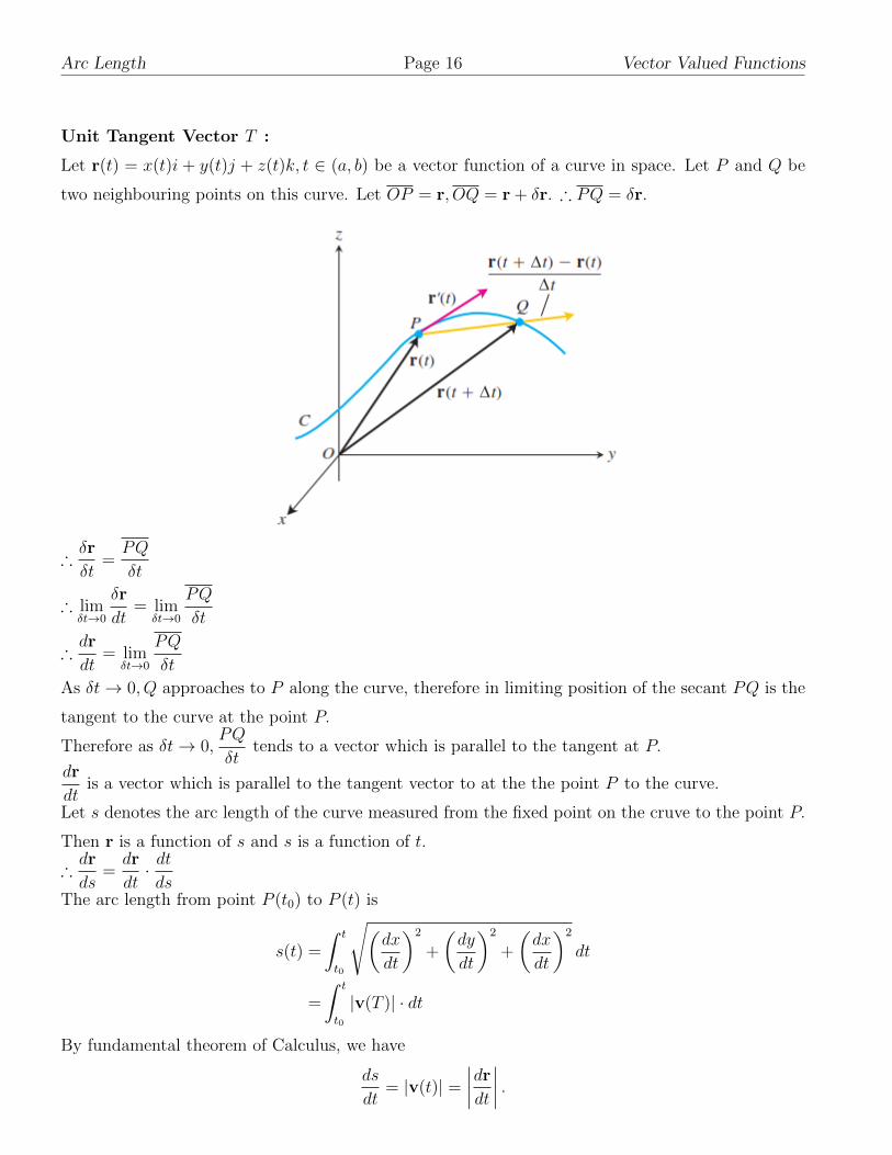
Unit Tangent Vector T :
Let r(t) = x(t)i + y(t)j + z(t)k, t ∈ (a, b) be a vector function of a curve in space. Let P and Q be
two neighbouring points on this curve. Let OP = r, OQ = r + δr. ∴ PQ = δr.
∴δr
δt=PQ
δt
∴ limδt→0
δr
dt= lim
δt→0
PQ
δt
∴dr
dt= lim
δt→0
PQ
δt
As δt→ 0, Q approaches to P along the curve, therefore in limiting position of the secant PQ is the
tangent to the curve at the point P.
Therefore as δt→ 0,PQ
δttends to a vector which is parallel to the tangent at P.
dr
dtis a vector which is parallel to the tangent vector to at the the point P to the curve.
Let s denotes the arc length of the curve measured from the fixed point on the cruve to the point P.
Then r is a function of s and s is a function of t.
∴dr
ds=dr
dt· dtds
The arc length from point P (t0) to P (t) is
s(t) =
∫ t
t0
√(dx
dt
)2
+
(dy
dt
)2
+
(dx
dt
)2
dt
=
∫ t
t0
|v(T )| · dt
By fundamental theorem of Calculus, we have
ds
dt= |v(t)| =
∣∣∣∣drdt∣∣∣∣ .
16

Vector Valued Functions Page 17 Arc Length
The velocity vector v =dr
dtis tangent to the curve and the vector
T =v
|v|=
dr
dt
|drdt|
is a unit vector tangent to the curve.
dr
ds=dr
dt· dtds
= v · 1
|v|= T
This equation says thatdr
dsis the unit tangent vector in the direction of the velocity v.
The unit tangent vector of a smooth curve r(t) is
T =dr
ds=
dr
dtds
dt
=v
|v|.
As particle moves along a smooth curve in the plane, T =dr
dsturns as the curve bends. Since T is
a unit vector, its length remains constant and only its direction changes as the particle moves along
the curve.
The rate at which T turns per unit of length along the curve is called the curvature. The curvature
of a curve is denoted by the Greek letter K (k’appa) and defined as if T is the unit vector of a curve,
the curvature function of the curve is
K =
∣∣∣∣dTds∣∣∣∣ .
If r(t) is a smooth curve then curvature can be calculated as:
K =
∣∣∣∣dTds∣∣∣∣ =
∣∣∣∣dTdt · dtds∣∣∣∣ =
1
|dsdt|·∣∣∣∣dTdt
∣∣∣∣=
1
|v|·∣∣∣∣dTdt
∣∣∣∣ , (∵ |v| = ds
dt
)where T =
v
|v|is the unit tangent vector.
Principal Unit Normal: As unit tangent vector T is of constant length, therefore T · dTds
= 0 i.e.
dT
dsis orthogonal to T. Hence the principal unit normal vector for a smooth curve in the plane is
N =
dT
ds∣∣∣∣dTds∣∣∣∣ We can calculate N as following:
17
Arc Length Page 18 Vector Valued Functions
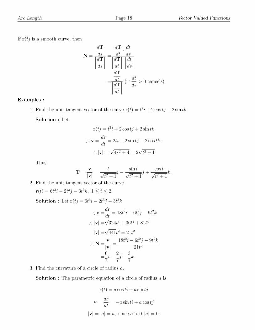
If r(t) is a smooth curve, then
N =
dT
ds∣∣∣∣dTds∣∣∣∣ =
dT
dt· dtds∣∣∣∣dTdt
∣∣∣∣ ∣∣∣∣ dtds∣∣∣∣
=
dT
dt∣∣∣∣dTdt∣∣∣∣ (∵
dt
ds> 0 cancels)
Examples :
1. Find the unit tangent vector of the curve r(t) = t2i+ 2 cos tj + 2 sin tk.
Solution : Let
r(t) = t2i+ 2 cos tj + 2 sin tk
∴ v =dr
dt= 2ti− 2 sin tj + 2 cos tk.
∴ |v| =√
4r2 + 4 = 2√t2 + 1
Thus,
T =v
|v|=
t√t2 + 1
i− sin t√t2 + 1
j +cos t√t2 + 1
k.
2. Find the unit tangent vector of the curve
r(t) = 6t3i− 2t3j − 3t3k, 1 ≤ t ≤ 2.
Solution : Let r(t) = 6t3i− 2t3j − 3t3k
∴ v =dr
dt= 18t2i− 6t2j − 9t2k
∴ |v| =√
324t4 + 36t4 + 81t4
|v| =√
441t2 = 21t2
∴ N =v
|v|=
18t2i− 6t2j − 9t2k
21t2
=6
7i− 2
7j − 3
7k.
3. Find the curvature of a circle of radius a.
Solution : The parametric equation of a circle of radius a is
r(t) = a cos ti+ a sin tj
v =dr
dt= −a sin ti+ a cos tj
|v| = |a| = a, since a > 0, |a| = 0.
18

Vector Valued Functions Page 19 Arc Length
The unit tangent vector of this curve is
T =v
|v|= − sin ti+ cos tj
dT
dt=− cos ti− sin tj∣∣∣∣dTdt∣∣∣∣ =√
cos2 t+ sin2 t = 1
Thus for any value of the parameter t, the curvature of a curve is
K =1
|v|·∣∣∣∣dTdt
∣∣∣∣ =1
a· 1 =
1
a.
4. Find T and N for the circular motion
r(t) = ti+ t2j.
Solution : Let
r(t) =ti+ t2j
v =dr
dt= i+ 2tj
|v| =√
1 + 4t2
∴ T =v
|v|=
i+ 2tj√1 + 4t2
dT
dt=
−4t
(1 + 4t2)3/2i+
2
(1 + 4t2)3/2j∣∣∣∣dTdt
∣∣∣∣ =
√16t2 + 4
(1 + 4t2)3=
2
1 + 4t2
N =
dT
dt∣∣∣∣dTdt∣∣∣∣ =
−2t√1 + 4t2
i+1√
1 + 4t2j.
Problem Set III
1. Find the arc length parameter along the curve
r(t) = cos ti+ sin tj + tk, from t = 0 to any point t.
2. Find the arc length parameter along the curve
r(t) = 4 cos ti+ 4 sin tj + 3tk, from t = 0 to t =π
2.
3. Find the curvature for the helix
r(t) = a cos ti+ a sin tj + btk, a, b ≥ 0 and a2 + b2 6= 0.
4. Find T and N for the plane curve
r(t) = (2t+ 3)i+ (5− t2)j, t > 0.
19

Exercise Page 20 Vector Valued Functions
5. Find T,N and curvature for the curve
r(t) = 2ti+ t2j +1
3tk, t > 0.
8. Exercise
1. If f(t) = t2i− tj + (2t+ 1)k, find limt→1
f(t).
2. Find limt→0
f(t) if exist, where
f(t) = ti− j, for t > 0= ti+ j, for t < 0.
3. Let
f(t) =
(sin 2t
3t+ a
)i+ (t2 + b)j, t > 0
= i+3
2j, t = 0
= (3 + c)i+ (2√t2 + 1 + d)j, t < 0.
Determine a, b, c, d so that f(t) is continuous at t = 0.
4. Discuss the continuity of the following function r(t) at t = 0, where
r(t) = e−t cos ti+ e−t sin tj + e−tk, if t 6= 0= i+ j + k, if t = 0.
5. A function f(t) is defined by
f(t) =
(t2 − 1
t− 1
)i+ t3j, t 6= 1
= 2i+ j, t = 1.
show that f(t) is continuous at t = 1.
6. Let r = r(t) and r = |r|, findd
dt
(r
r
).
7. If r(t) = a coswt + b sinwt, show that r × dr
dt= wa × b and
d2r
dt2= −w2r, where a,b and
w are constants.
8. Show that r = e−t(a cos 2t + b sin 2t), where a,b are constant vectors is a solution of the
differential equationd2r
dt2+ 2
dr
dt+ 5r = 0.
9. Find the unit tangent vector of the curve
r(t) = (2 + t)i− (t+ 1)j + tk, 0 ≤ t ≤ 3.
10. Find the arc length along the curve
r(t) = 6 sin 2ti+ 6 cos 2tj + 5tk, from t = 0 to t = π.
11. Find the unit tangent vector and the curvature at a point P (x, y, z) on the curve
x = 3 cos t, y = 3 sin t, z = 4t.
20

Vector Valued Functions Page 21 Answers
12. Evaluate∫ 2
1[(6− 6t)i+ 3
√tj +
4
t2k] dt.
13. Evaluate∫ 4
1
[1
ti+
1
5− tj +
1
2tk
]dt.
9. Answers
Problem Set I
1. 5i + 5j + 7k 2. 0 3. f is continuous 4. f is continuous
Problem Set II
1. i +√
2j + k 2. −i + 6k 3.
(dr
dt
)t=π
4
= − 1√2i + 1√
2j + 2k, |
(dr
dt
)|t=π
4=√
5
4.dr
dt= sin ti + (1− cos t)j,
d2r
dt2= cot ti + sin tj
7.
[rd2r
dt2d3r
dt3
]+
[rdr
dt
d4r
dt4
]Problem Set III
1.√
2t 2. 5t 3. κ =a
a2 + b24. T =
1√1 + t2
i− 1√1 + t2
j, N = − 1√1 + t2
i− 1√1 + t2
j, κ =1
2(1 + t2)3/2
5. T = − 4t
(t2 + 2)2i +
4− 2t2
(t2 + 2)2j− 4t
(t2 + 2)2k, N = − 2t
t2 + 2i +
2− t2
t2 + 2j− 2t
t2 + 2k, κ =
2
(t2 + 2)2
Exercise
1. i− j + 3k 2.limit exists and limt→0
f(t) = 0 3. a = 1/3, b = 3/2, c = −2, d = −7/6 4. not continuous
9. 1√3(i− j + k) 10. 13π
11. T = −3 sin t
5i +
3 cos t
5j +
4
5k, N = − cos ti− sin tj, κ =
3
2513. ln 2(2i− 2j + k)
21


CHAPTER 2
Line Integrals
Introduction
In the previous chapter we considered integration of vector function of scalar variable as antideriva-
tive.In this section we discuss the integrals along curves in 2 or 3 dimensional space.
Curves in space: We have seen that any equation of the form r(t) = x(t)i+y(t)j+z(t)k, a ≤ t ≤ b
represents a curve in space.The vectordr
dt=dx
dti +
dy
dtj +
dz
dtk is the tangent vector to this curve.
A curve C defined by r(t) = x(t)i + y(t)j + z(t)k, a ≤ t ≤ b is said to smooth if the function r has
continuous non-zero first derivative at every point in [a, b].
1. Definition and Evaluation of Line Integral
Suppose that f(x, y, z) is a function whose domain contains the curve
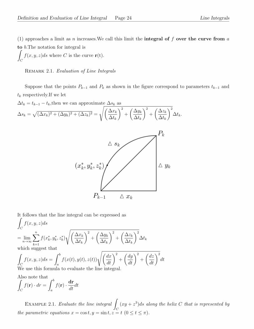
r(t) = x(t)i + y(t)j + z(t)k, a ≤ t ≤ b.We divide the curve into n sub
arcs by the points P0(t0), P1(t1), · · · , Pn(tn) as shown in the figure,where a = t0 < t1 < · · · < tn = b
Suppose the coordinates of Pk are (xk, yk, zk) .The typical sub arc has length ∆sk.In each sub arc we
choose a point (x∗k, y∗k, z∗k) as shown in the figure.Note the approximation ∆Ak = f(x∗k, y
∗k, z∗k)∆sk
Consider the sum
Sn =n∑k=1
f(x∗k, y∗k, z∗k)∆sk . . . (1)
If f is continuous and the functions x(t), y(t), z(t) have continuous first derivatives,then the sum in
23
Definition and Evaluation of Line Integral Page 24 Line Integrals
(1) approaches a limit as n increases.We call this limit the integral of f over the curve from a
to b.The notation for integral is∫C
f(x, y, z)ds where C is the curve r(t).
Remark 2.1. Evaluation of Line Integrals
Suppose that the points Pk−1 and Pk as shown in the figure correspond to parameters tk−1 and
tk respectively.If we let
∆tk = tk−1 − tk,then we can approximate ∆sk as
∆sk =√
(∆xk)2 + (∆yk)2 + (∆zk)2 =
√(∆xk∆tk
)2
+
(∆yk∆tk
)2
+
(∆zk∆tk
)2
∆tk.
It follows that the line integral can be expressed as∫C
f(x, y, z)ds
= limn→∞
n∑k=1
f(x∗k, y∗k, z∗k)
√(∆xk∆tk
)2
+
(∆yk∆tk
)2
+
(∆zk∆tk
)2
∆tk
which suggest that∫C
f(x, y, z)ds =
∫ b
a
f(x(t), y(t), z(t))
√(dx
dt
)2
+
(dy
dt
)2
+
(dz
dt
)2
dt
We use this formula to evaluate the line integral.
Also note that∫C
f(r) · dr =
∫ b
a
f(r) · dr
dtdt
Example 2.1. Evaluate the line integral
∫C
(xy + z3)ds along the helix C that is represented by
the parametric equations x = cos t, y = sin t, z = t (0 ≤ t ≤ π).
24

Line Integrals Page 25 Definition and Evaluation of Line Integral
Solution. By the definition of line integral,∫C
(xy + z3)ds
=
∫ π
0
(cos t sin t+ t3)
√(dx
dt
)2
+
(dy
dt
)2
+
(dz
dt
)2
dt
=
∫ π
0
(cos t sin t+ t3)√
(− sin t)2 + (cos t)2 + 1dt
=√
2
∫ π
0
(cos t sin t+ t3)dt
=√
2
[sin2 t
2+t4
4
]π0
=
√2π4
4
Example 2.2. Evaluate the line integral
∫C
(x− 3y2 + z)ds
from (0, 0, 0) to (1, 1, 1) along the line segment C.
Solution. The equations of a line passing through the points (0, 0, 0) and (1, 1, 1) are x = y =
z.Ifx = t,then y = t and z = t.Therefore the parametric equations of C are x = t, y = t, z = t
(0 ≤ t ≤ 1).By the definition of line integral∫C
(x− 3y2 + z)ds
=
∫ 1
0
(t− 3t2 + t)
√(dx
dt
)2
+
(dy
dt
)2
+
(dz
dt
)2
dt
=
∫ 1
0
(t− 3t2 + t)√
3dt
=√
3
∫ 1
0
(2t− 3t2)dt
=0
Example 2.3. If f = (2y + 3)i + (xz)j + (yz − x)k,then evaluate
∫C
f(r) · dr along the path
C : r(t) = 2t2i + tj + t3k from t = 0 to 1
Solution. By the Remark 2.1∫C
f(r) · dr =
∫ 1
0
f(r) · dr
dtdt Along C: x = 2t2, y = t, z = t3.
25

Mass and Moment Page 26 Line Integrals
Therefore along C: f = (2t+ 3)i + (2t2)t3j + (tt3 − 2t3)k∫C
f(r) · dr
=
∫ 1
0
[(2t+ 3)i + 2t5j + (t4 − 2t3)k] · ddt
(2t2i + tj + t3k)dt
=
∫ 1
0
(3t6 + 2t5 − 6t4 + 8t2 + 12t)dt
=288
7
Remark 2.2. Additivity
If a curve C is made by joining a finite number of smooth curves C1, C2, . . . , Cn end to end,then
the integral of a function f over C is the sum of the integrals over the curves that make it up:∫C
f(x, y, z)ds
=
∫C1
f(x, y, z)ds+
∫C2
f(x, y, z)ds+ · · ·+∫Cn
f(x, y, z)ds.
Example 2.4. Suppose C1 and C2 are the line segments from the origin to (1, 1, 0) and from
(1, 1, 0) to (1, 1, 1) respectively.If C = C1 ∪ C2,then integrate f(x, y, z) = x− 3y2 + z over C.
Solution. The parametrizations for C1 and C2:
C1:x = t, y = t, z = 0 (0 ≤ t ≤ 1).
C2:x = 1, y = 1, z = t (0 ≤ t ≤ 1).
By Remark 2.2 ∫C
f(x, y, z)ds =
∫C1
f(x, y, z)ds+
∫C2
f(x, y, z)ds.
=
∫ 1
0
(t− 3t2 + 0)√
2dt+
∫ 1
0
(1− 3 + t)(1)dt
=√
2
[t2
2− t3
]1
0
+
[t2
2− 2t
]1
0
=− 3 +√
2
2.
2. Mass and Moment
Mass of a Wire as a Line Integral
Consider a wire that is bent in the shape of a curve C.If the composition of a wire is uniform so
that its mass is distributed uniformly,then the wire is said to be homogeneous. We define the linear
mass density of the wire to be the total mass divided by the total length.However,if the mass of
a wire is not uniformly distributed,then the linear mass density is not a useful measure. Because
26

Line Integrals Page 27 Mass and Moment
it does account for variation in mass concentration.In such case we describe the mass concentration
at a point by a Mass density function δ.It can be viewed as a limit: δ = lim∆t→0
∆M
∆s.· · · (2) Here
∆M and ∆s denote the mass and length of a small section of wire centered at the point as shown in
the figure. Note that ∆M/∆s is the linear mass density of the small section of wire.Therefore the
mass density function at a point can be viewed as the limit of the linear mass densities of small wire
sections centered at the point. Suppose that δ = δ(x, y, z) is the density function for a smooth wire
C.Assume that the wire is subdivided in to n small sections.
Let (x∗k, y∗k, z∗k) be the centre of the kth section.Suppose ∆Mk and ∆sk are the mass and length of the
kth section respectively.Hence from (2) it follows that the mass of kth section can be approximated
as
∆Mk = δ(x∗k, y∗k, z∗k)∆sk
Therefore the mass M of the entire wire can be approximated as
M =n∑k=1
δ(x∗k, y∗k, z∗k)∆sk
If we increase n,then we get exact value of M .
M = limn→∞
n∑k=1
δ(x∗k, y∗k, z∗k)∆sk =
∫C
δ(x, y, z)ds
Example 2.5. A coil spring lies along the helix r(t) = cos 4ti + sin 4tj + tk, 0 ≤ t ≤ 2π.
The spring’s density is given by δ(x, y, z) = x2 + y2 + 2z.Find the spring’s mass.
27
Mass and Moment Page 28 Line Integrals
Solution. The spring’s mass is given by
M =
∫C
δ(x, y, z)ds
=
∫ 2π
0
(sin2 4t+ cos2 4t+ 2t)
√(dx
dt
)2
+
(dy
dt
)2
+
(dz
dt
)2
dt
=
∫ 2π
0
(1 + 2t)√
17dt
=√
17[t+ t2
]2π0
=2√
17π(1 + 2π)
Moment and The Centre of Mass
Children on a see-saw learn by experience that a lighter child can balance a heavier one by seating
farther from the fulcrum point. This is because tendency for an object to produce rotation is
proportional not only to its mass but also to the distance between the object and fulcrum. Consider
an x-axis,which we view as a weightless beam .If a point mass m is located on the axis at x,then the
tendency for that mass to produce a rotation of the beam about a point a on the axis is called the
moment of m about x = a. A weightless beam along the axis will rotate clockwise about a,rotate
counter-clockwise about a,or balance perfectly.If it balance perfectly,then the system is said to be in
equilibrium;and in this case a is called the centre of mass.
The Coordinates of the Centre of Mass
The coordinates of the centre of mass of a wire lying along a smooth curve C in space whose density
is δ(x, y, z) are given by:
x = Myz/M, y = Mxz/M, z = Mxy/M .
Here Myz =
∫C
xδ(x, y, z)ds,Mxz =
∫C
yδ(x, y, z)ds
Mxy =
∫C
zδ(x, y, z)ds and M =
∫C
δ(x, y, z)ds
Example 2.6. A metal wire lies along the semicircle y2 + z2 = 1, z ≥ 0 in the yz−plane.Find
the centre of wire’s mass if the density at the point (x, y, z) of the metal wire is δ(x, y, z) = 2− z
Solution. Suppose (x, y, z) are the coordinates of the centre of mass
.Here x = 0 and y = 0 because the metal wire lies in the yz-plane.
Parametric equations of the wire are
28

Line Integrals Page 29 Mass and Moment
x = 0, y = cos t, z = sin t (0 ≤ t ≤ π).We have z = Mxy/M .
M =
∫C
δ(x, y, z)ds
=
∫ π
0
(2− sin t)
√(dx
dt
)2
+
(dy
dt
)2
+
(dz
dt
)2
dt
=
∫ π
0
(2− sin t)dt
=2π − 2
Mxy =
∫C
zδ(x, y, z)ds
=
∫ π
0
sin t(2− sin t)
√(dx
dt
)2
+
(dy
dt
)2
+
(dz
dt
)2
dt
=
∫ π
0
(2 sin t− sin2 t)dt
=(8− π)/2
z = Mxy/M = (8− π)/(4π − 4).Therefore the centre of mass is
(0, 0, (8− π)/(4π − 4))
Problem Set I
(1) Evaluate
∫C
xds,where C is the parabolic curve x = t, y = t2 from (0, 0) to (2, 4)
(2) Find the line integral of f(x.y) = yex2
along the curve
r(t)= 4ti− 3tj,−1 ≤ t ≤ 2
(3) Find the mass of a thin wire shaped in the form of the circular arc y =√
9− x2, (0 ≤ x ≤ 3)
if the density function is δ(x, y) = x√y.
(4) Evaluate
∫C
(xy+y+z)ds along the curve
r(t)= 2ti + tj + (2− 2t)k, 0 ≤ t ≤ 1
(5) Find the line integral of f(x.y) = x3/y
along the curve C : y = x2/2, 0 ≤ x ≤ 2
(6) A wire of density δ(x, y, z) = 15√y + 2 lies along the curve r(t)= (t2 − 1)j + 2tk,−1 ≤ t ≤
1.Find its centre of mass.
(7)
∫C
x dx+y dy where C is the ellipse x2 + 4y2 = 4.
(8) Evaluate
∫C
F· dr for the vector field F = yi−xj counter clockwise along the circle x2+y2 = 1
from (1, 0) to (0, 1).
29

Work,Circulation and Flux Page 30 Line Integrals
3. Work,Circulation and Flux
In this section we will consider functions that associates vectors with points in two-space or
three-space.
Definition 2.1. (Vector Field) A vector field is a function that associates a unique vector
V (P ) with each point P in a region of 2-space or 3-space.
Remark 2.3. Note that in this definition there is no reference to a coordinate system. However,for
computational purposes we introduce a coordinate system so that vectors can be assigned components.
If V (P ) is a vector field in an xy−coordinate system,then the point P will have some coordinates
(x, y),and the associated vector will have components that are functions of x and y. Hence the vector
field can be expressed as
F (x, y) = f(x, y)i + g(x, y)j
Similarly,in 3-space with an xyz-coordinate system a vector field can be expressed as
F (x, y, z) = f(x, y, z)i + g(x, y, z)j + h(x, y, z)k
Some examples of vector fields
A vector field is continuous if the component functions f, g and h are continuous;and differen-
tiable if f, g and h are differentiable.
The Work Done by a Force
The work done by a constant force We know that the work W done by a constant force of
magnitude F acting on an object that moves along a line is given by W = Fd=force× distance.
Remark 2.4. If we let F a force vector of magnitude |F| = F acting in the direction of mo-
tion,then we can write W as W = |F| d.Also if we assume that object moves along a line from point
P to point Q,then d =∣∣PQ∣∣,and we can write W as W = |F|
∣∣PQ∣∣.
30

Line Integrals Page 31 Work,Circulation and Flux
Remark 2.5. The vector PQ is called the displacement vector for the object.If a constant force F
is not in the direction of motion,but makes an angle θ with the displacement,then the work W done
by F is given by W = |F| cos θ∣∣PQ∣∣ = |F| ·
∣∣PQ∣∣.Work done by a Variable Force along a Curved Path
Now we define a more general concept of the work performed by a variable force acting on a particle
that moves along a curved path. Suppose a particle moves along a smooth parametric curve C
through a continuous force field F.Assume that the particle moves along C from a point A to a
point B as the parameter increases.Divide C in to n arcs by inserting distinct points P1, P2, . . . , Pn−1
between A and B in the direction of increasing parameter.Denote the length of the kth arc by ∆sk.
Let (x∗k, y∗k, z∗k) be any point on the kth arc.Suppose T ∗k = T (x∗k, y
∗k, z∗k) is the unit tangent vector;and
F ∗k = F (x∗k, y∗k, z∗k) is the force vector at (x∗k, y
∗k, z∗k).
If the kth arc is small,then the force will not vary much.Therefore we can approximate the force by
the constant value F ∗k on this arc.Also the direction of motion will not vary much over the small
arc,so we can assume that the particle moves in the direction of T ∗k for a distance of ∆sk;that is,the
particle has a linear displacement ∆skT∗k .Hence by the definition of work,it follows that the work
∆Wk done by the vector field along the kth arc can be approximated as
∆Wk = F ∗k · (∆skT ∗k ) = F ∗k · T ∗k∆sk
The total work W done by the vector field as the particle moves along C from A to B can be
approximated as
W =n∑k=1
(F ∗k · T ∗k )∆sk
If we increase n,then the error in the approximation approaches to zero.Thus the exact work done
by the vector field is
31

Work,Circulation and Flux Page 32 Line Integrals
W = limn→∞
n∑k=1
(F ∗k · T ∗k )∆sk =
∫C
F(x, y, z) ·T(x, y, z)ds
We know that the tangent vector T is expressed as
T =dr
ds,where C is the curve r(t).
This suggest that W can be expressed as
W =
∫C
F(x, y, z) · drdsds =
∫C
F(x, y, z) · dr
Remark 2.6. If F is a continuous vector field and C = r(t) is a smooth curve,then the work
done by the vector field along C in the increasing direction of parameter is
W =
∫C
F · dr
Example 2.7. Find the work done by F= (y − x2)i + (z − y2)j + (x − z2)k along the curve
r(t) = ti + t2j + t3k, 0 ≤ t ≤ 1.
Solution. The work W done by F along C is given by
W =
∫C
F (x, y, z) · dr
=
∫ 1
0
F (x(t), y(t), z(t)) · drdtdt
=
∫ 1
0
((t2 − t2)i + (t3 − t4)j + (t− t6)k) · (i + 2tj + 3t2k)dt
=
∫ 1
0
(t3 − t4)(2t) + (t− t6)(3t2)dt
=
∫ 1
0
(2t4 − 2t5 + 3t3 − 3t8)dt
Work=29
60Flow Integrals and Circulations
If r(t), a ≤ t ≤ b is a smooth curve in the domain of a continuous velocity field F,then the flow along
the curve is given by
Flow=
∫ b
a
F ·Tds =
∫ b
a
F · drdtdt
The integral
∫ b
a
F ·Tds is called a flow integral.If the curve is a closed loop,then the flow is called
the circulation around the curve.
Example 2.8. A velocity field is F=xi + zj + yk.Find the flow along the curve r(t) = cos ti +
sin tj + tk, 0 ≤ t ≤ π/2.
32

Line Integrals Page 33 Work,Circulation and Flux
Solution. By the definition of flow
Flow =
∫ b
a
F · Tds
=
∫ π/2
0
F · drdtdt
=
∫ π/2
0
(cos ti + tj + sin tk)((− sin t)i + (cos t)j + k)dt
=
∫ π/2
0
(− sin t cos t+ t cos t+ sin t)dt
=π − 1
2
Flux Across a Plane Curve
If C is a smooth curve in the domain of a continuous vector field F(x, y) = M(x, y)i + N(x, y)j in
the plane,and if n is the outward pointing unit normal vector on C,the flux of F across C is given
by∫C
F · ndsIt is easy to see that
F · n = M(x, y)dy
ds−N(x, y)
dx
ds
Flux of F across C =
∫C
M dy-N dx
Example 2.9. Find the flux of F=(x-y)i+xj across the circle x2 + y2 = 1
Solution. Suppose is the circle x2 + y2 = 1 .The parametric form is C : x = cos t, y = sin t, 0 ≤t ≤ 2π.Here M = x− y = cos t− sin t, N = x = cos t
Flux of F across C is given by
Flux =
∫C
Mdy −Ndx
=
∫ 2π
0
{(cos t− sin t) cos t+ cos t sin t}dt
=
∫ 2π
0
cos2 tdt
=
∫ 2π
0
1 + cos 2t
2dt
=π
The flux of F across the circle is π.
33
Path Independence,Potential Functions Page 34 Line Integrals
Problem Set II
(1) Find the work done by the force field F(x,y)= xyi + x2j on a particle that moves along the
curve C : x = y2 from (0, 0) to (1, 1).
(2) Find the circulation and flux of the vector fields F1(x,y)= xi + yj and F2(x,y)= −yi + xj
around and across each of the following curves.
(a) The circle r(t)= cos ti + sin tj, (0 ≤ t ≤ 2π).
(b) The ellipse r(t)= cos ti + 4 sin tj, (0 ≤ t ≤ 2π).
(3) Find the work done by F over the curve in the direction of increasing t
(a) F = xyi + yj− yzk and r(t)= ti + t2j + tk, 0 ≤ t ≤ 1
(b) F = zi + xj + yk and r(t)= sin ti + cos tj + tk, 0 ≤ t ≤ 2π
4. Path Independence,Potential Functions
We will study properties of vector fields that relate to the work they perform on particles moving
along various curves.For certain kinds of vector fields work done on a moving particle along a curve
depends only on the endpoints of the curve and not on the curve itself.Such vector fields are of
special importance in physics and engineering. Let F be a field defined on an open region D in
space.Suppose that for any two points A and B in D the work
∫ B
A
F · dr done in moving from A to
B is the same over all paths from A to B. Then the integral
∫F · dr is path independent in D
and the field F is conservative on D.
Gradient Fields
The gradient field of a differentiable function f(x, y, z) is the field of vectors∂f
∂xi +
∂f
∂yj +
∂f
∂zk.
We denote it as ∇f .
∇f =∂f
∂xi +
∂f
∂yj +
∂f
∂zk
Example 2.10. Find the gradient field of f(x, y, z) = xyz.
Solution. The gradient field of f is
∇f =∂f
∂xi +
∂f
∂yj +
∂f
∂zk = yzi + xzj + xyk
34

Line Integrals Page 35 Path Independence,Potential Functions
Example 2.11. Sketch the gradient field of φ(x, y) = x+ y.
Solution. The gradient field of φ is
∇φ =∂φ
∂xi +
∂φ
∂yj = i + j
Potential Function:If F is a field defined on D and F= ∇f for some scalar function f on D, then
f is called a potential function for F.
Theorem 2.1. Let F be a vector field whose components are continuous throughout an open
connected region D in space.If there exists a differentiable function f such that F = ∇f ,then for all
points A and B in D the value of
∫ B
A
F · dr is independent of the path from A to B in D.
Proof. Suppose that A and B are two points in D.
C : r(t) = g(t)i + h(t)j + k(t)k, a ≤ t ≤ b is a smooth curve in D joining A and B. Along the curve
C,f is a differentiable function of t.By chain rule,we get
df
dt=∂f
∂x
dx
dti +
∂f
∂y
dy
dtj +
∂f
∂z
dz
dtk
=(∂f
∂xi +
∂f
∂yj +
∂f
∂zk) · (dx
dti +
dx
dtj +
dx
dtk)
=∇f · drdt
=F · drdt, becauseF = ∇f
Hence,
∫C
F · dr =
∫ b
a
F · drdtdt
=
∫ b
a
df
dtdt
= [f(g(t), h(t), k(t))]ba
=f(B)− f(A)
35

Path Independence,Potential Functions Page 36 Line Integrals
Therefore the value integral depends only on the values of f at A and B and not on the path in
between.
Remark 2.7. The converse of this theorem is true;i·e· if for all points A and B in D the value
of
∫ B
A
F · dr is independent of the path from A to B in D,then there exists a differentiable function
f such that F = ∇f .
Remark 2.8. If the integral is independent of the path from A to B,then its value is
∫ B
A
F ·dr =
f(B)− f(A).
Theorem 2.2. The following statements are equivalent:
1.∫
F · dr = 0 around every closed loop in D.
2. The field F is conservative on D.
Proof. (1)⇒ (2)
To show that the field F is conservative,for this it is sufficient to show that for any two points A and
B in D the integral of F · dr has the same value over any two paths C1 and C2 from A to B.
We reverse the direction on C2 to make a path −C2 from B to A.Observe that together C1 and −C2
make a closed loop C(see the fig). We have,
∫C1
F·dr−∫C2
F·dr =
∫C1
F·dr+
∫−C2
F·dr =
∫C
F·dr = 0
Therefore
∫C1
F · dr =
∫C2
F · dr
Hence the integrals over C1 and C2 give the same value.
(2)⇒(1)
Now assume that the field F is conservative.We want to show that the integral of F · dris zero over
any closed loop C.Choose any two different points A and B on C.We use these points to break C in
two pieces,C1 from A in to B followed by C2 from B back to A.
36

Line Integrals Page 37 Path Independence,Potential Functions
∫C
F · dr =
∫C1
F · dr +
∫C2
F · dr =
∫ B
A
F · dr−∫ B
A
F · dr = 0
Remark 2.9. Let F= M(x, y, z)i+N(x, y, z)j+P (x, y, z)k be a field whose component functions
have continuous first order partial derivatives. Then F is conservative if and only if∂P
∂y=∂N
∂z,∂M
∂z=∂P
∂xand
∂N
∂x=∂M
∂yWhen we know that F is conservative,we usually find a potential function for F.It requires solving
the equation
∇f = F or∂f
∂xi +
∂f
∂yj +
∂f
∂zk = Mi +Nj + Pk
Therefore f can be obtained by integrating the equations∂f
∂x= M,
∂f
∂y= N,
∂f
∂z= P .
Example 2.12. Show that F=(ex cos y + yz)i + (xz − ex sin y)j + (xy + z)k is conservative and
find a potential function for it.
Solution. Comparing F=(ex cos y + yz)i + (xz − ex sin y)j + (xy + z)k with F= M i +N j + Pk
we have
M = ex cos y + yz,N = xz − ex sin y, P = xy + z∂P
∂y= x =
∂N
∂z,∂M
∂z= y =
∂P
∂x,∂N
∂x= −ex sin y + z =
∂M
∂yBy Remark 2.9 F is conservative and we can find a potential function f by integrating the equations∂f
∂x= ex cos y + yz,
∂f
∂y= xz − ex sin y,
∂f
∂z= xy + z
We integrating the first equation with respect to x,keeping y and z constant.
f(x, y, z) = ex cos y + xyz + g(y, z)
We write the constant of integration as a function of y and z.Now we can find∂f
∂yfrom this equation
and equate it with the expression∂f
∂y.
−ex sin y + xz +∂g
∂y= xz − ex sin y
37

Path Independence,Potential Functions Page 38 Line Integrals
From the last equation we get,∂g
∂y= 0.Therefore g is a function of z alone,say h(z).
f(x, y, z) = ex cos y + xyz + h(z)
We now calculate∂f
∂zfrom this equation and
equate it to the expression∂f
∂z.
xy +dh
dz= xy + z.It gives
dh
dz= z.So h(z) = z2/2 + C
Hence f(x, y, z) = ex cos y + xyz + z2/2 + k.
Remark 2.10. Let F= M(x, y)i+N(x, y)j be a field whose component functions have continuous
first order partial derivatives. Then F is conservative if and only if∂M
∂y=∂N
∂xWhen we know that F is conservative,we usually find a potential function for F.It requires solving
the equation
∇f = F or∂f
∂xi +
∂f
∂yj = Mi +Nj
Therefore f can be obtained by integrating the equations∂f
∂x= M,
∂f
∂y= N .
Example 2.13. Show that F=2xy3i + (1 + 3x2y2)j is conservative and find a potential function
for it.
Solution. Comparing F=2xy3i + (1 + 3x2y2)j with F= M i +N j we have
M = 2xy3, N = 1 + 3x2y2.We get,∂M
∂y= 6xy2 =
∂N
∂xBy Remark 2.10 F is conservative and we can find a potential function f by integrating the equations∂f
∂x= 2xy3,
∂f
∂y= 1 + 3x2y2
We integrating the first equation with respect to x,keeping y constant.f(x, y) = x2y3 + g(y). We
write the constant of integration as a function of y.Now we can find∂f
∂yfrom this equation and
equate it with the expression∂f
∂y.Therefore 3x2y2 +
dg
dy= 1 + 3x2y2
From the last equation we get,dg
dy= 1.Therefore g(y) = y + k.Hence f(x, y) = x2y3 + y + k. We will
define two important operations on a vector field: the divergence and the curl
Definition 2.2. If F(x, y, z) = f(x, y, z)i + g(x, y, z)j + h(x, y, z)k,then the divergence of F
is denoted by divF and is defined by
divF =∂f
∂x+∂g
∂y+∂h
∂z
38

Line Integrals Page 39 Path Independence,Potential Functions
The del operator allows us to express the divergence of a vector field
F(x, y, z) = f(x, y, z)i + g(x, y, z)j + h(x, y, z)k
divF = ∆ · F =∂f
∂x+∂g
∂y+∂h
∂z
Definition 2.3. If F(x, y, z) = f(x, y, z)i+g(x, y, z)j+h(x, y, z)k,then the curl of F is denoted
by curlF and is defined by
curlF = (∂h
∂y− ∂g
∂z)i + (
∂f
∂z− ∂h
∂x)j + (
∂g
∂x− ∂f
∂y)k
We express the curlF as
curlF=∆× F=
∣∣∣∣∣∣∣i j k∂
∂x
∂
∂y
∂
∂zf g h
∣∣∣∣∣∣∣Example 2.14. Find the divergence and the curl of the vector field
F(x, y, z) = x2yi + 2y3zj + 3zk
Solution. By the definition of divergence
divF =∂
∂x(x2y) +
∂
∂y(2y3z) +
∂
∂z(3z)
divF = 2xy + 6y2z + 3
By the definition of curl
curlF=∆× F=
∣∣∣∣∣∣∣i j k∂
∂x
∂
∂y
∂
∂zx2y 2y3z 3z
∣∣∣∣∣∣∣curlF = −2y3i− x2k
Problem Set III
(1) Find the gradient fields of the following functions
(a) f(x, y, z) = ez − ln(x2 + y2)
(b) f(x, y, z) = ln√x2 + y2 + z2
(c) f(x, y, z) = xy + yz + xz
(2) In each of the following determine whether F is a conservative vector field.If so,find a po-
tential function for it.
(a) F(x, y) = xi + yj.
(b) F(x, y) = x2yi + 5xy2j.
(c) F(x, y) = (cos y + y cosx)i + (sinx− x sin y)j.
(3) Show that each of the following integral is independent of the path,and use Remark 2.8 to
find its value.
(a)
∫ (2,3,−6)
(0,0,0)
2xdx+ 2ydy + 2zdz.
39
Green’s Theorem in Plane Page 40 Line Integrals
(b)
∫ (1,2,3)
(0,0,0)
2xydx+ (x2 − z2)dy − 2yzdz.
(c)
∫ (0,1,1)
(1,0,0)
sin y cosxdx+ cos y sinxdy + dz.
5. Green’s Theorem in Plane
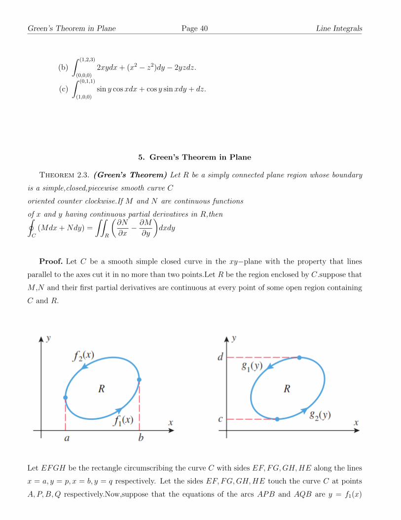
Theorem 2.3. (Green’s Theorem) Let R be a simply connected plane region whose boundary
is a simple,closed,piecewise smooth curve C
oriented counter clockwise.If M and N are continuous functions
of x and y having continuous partial derivatives in R,then∮C
(Mdx+Ndy) =
∫∫R
(∂N
∂x− ∂M
∂y
)dxdy
Proof. Let C be a smooth simple closed curve in the xy−plane with the property that lines
parallel to the axes cut it in no more than two points.Let R be the region enclosed by C.suppose that
M ,N and their first partial derivatives are continuous at every point of some open region containing
C and R.
Let EFGH be the rectangle circumscribing the curve C with sides EF, FG,GH,HE along the lines
x = a, y = p, x = b, y = q respectively. Let the sides EF, FG,GH,HE touch the curve C at points
A,P,B,Q respectively.Now,suppose that the equations of the arcs APB and AQB are y = f1(x)
40

Line Integrals Page 41 Green’s Theorem in Plane
and y = f2(x) respectively.Then we have∫∫R
∂M
∂ydxdy =
∫ b
a
[∫ f2(x)
f1(x)
∂M
∂ydy
]dx
=
∫ b
a
[M(x, y)]f1(x)f2(x)dx
=
∫ b
a
[M(x, f2(x))−M(x, f1(x))]dx
=
∫ b
a
M(x, f2(x))dx−∫ b
a
M(x, f1(x))dx
=−∫ a
b
M(x, f2(x))dx−∫ b
a
M(x, f1(x))dx
=−[∫
arcAPB
Mdx+
∫arcBQA
Mdx
]=−
∮C
Mdx
Therefore
∮C
Mdx = −∫∫
R
∂M
∂ydxdy · · · (1) Next suppose that the equations of the
arcs PAQ and PBQ are x = g1(y) and x = g2(y) respectively.Then we have∫∫R
∂N
∂xdxdy =
∫ q
p
[∫ g2(y)
g1(y)
∂N
∂xdx
]dy
=
∫ q
p
[N(x, y)]g1(y)g2(y)dy
=
∫ q
p
[N(f2(y), y)−N(g1(y), y)]dy
=
∫ q
p
N(g2(y), y)dy −∫ q
p
N(g1(y)), ydy
=
∫ q
p
N(g2(y), y)dy +
∫ p
q
N(g1(y), y)dy
=
[∫arcPBQ
Ndy +
∫arcQAP
Ndy
]=
∮C
Ndy
Therefore
∮C
Ndy =
∫∫R
∂N
∂xdxdy · · · (2)
Adding (1) and (2),we get∮C
(Mdx+Ndy) =
∫∫R
(∂N
∂x− ∂M
∂y
)dxdy
Remark 2.11. Green’s Theorem for Multiply Connected Region
41
Green’s Theorem in Plane Page 42 Line Integrals
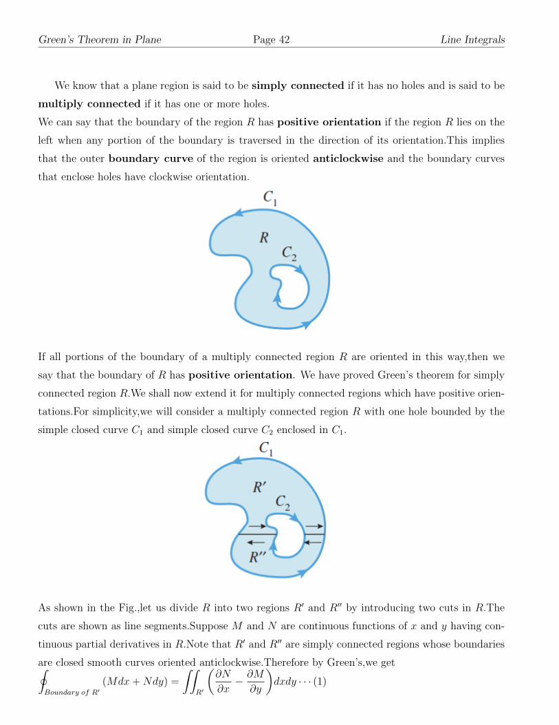
We know that a plane region is said to be simply connected if it has no holes and is said to be
multiply connected if it has one or more holes.
We can say that the boundary of the region R has positive orientation if the region R lies on the
left when any portion of the boundary is traversed in the direction of its orientation.This implies
that the outer boundary curve of the region is oriented anticlockwise and the boundary curves
that enclose holes have clockwise orientation.
If all portions of the boundary of a multiply connected region R are oriented in this way,then we
say that the boundary of R has positive orientation. We have proved Green’s theorem for simply
connected region R.We shall now extend it for multiply connected regions which have positive orien-
tations.For simplicity,we will consider a multiply connected region R with one hole bounded by the
simple closed curve C1 and simple closed curve C2 enclosed in C1.
As shown in the Fig.,let us divide R into two regions R′ and R′′ by introducing two cuts in R.The
cuts are shown as line segments.Suppose M and N are continuous functions of x and y having con-
tinuous partial derivatives in R.Note that R′ and R′′ are simply connected regions whose boundaries
are closed smooth curves oriented anticlockwise.Therefore by Green’s,we get∮Boundary of R′
(Mdx+Ndy) =
∫∫R′
(∂N
∂x− ∂M
∂y
)dxdy · · · (1)
42
Line Integrals Page 43 Green’s Theorem in Plane
∮Boundary of R′′
(Mdx+Ndy) =
∫∫R′′
(∂
∂x− ∂M
∂y
)dxdy · · · (2)
Adding (1) and (2),we get∮Boundary of R′
(Mdx+Ndy) +
∮Boundary of R′′
(Mdx+Ndy)
=
∫∫R′
(∂N
∂x− ∂M
∂y
)dxdy +
∫∫R′′
(∂N
∂x− ∂M
∂y
)dxdy
=
∫∫R
(∂N
∂x− ∂M
∂y
)dxdy
The two line integrals are taken in opposite directions along the cuts,
and hence cancel there,leaving only the contributions along C1 and C2.
Thus,we get∮C1
(Mdx+Ndy) +
∮C2
(Mdx+Ndy) =
∫∫R
(∂N
∂x− ∂M
∂y
)dxdy
This is an extension of Green’s theorem to a multiply connected region with one hole. More gener-
ally,if R is a multiply connected region with n holes,then along of (3) involves n + 1 integrals,one
taken anticlockwise around the outer boundary of R and the rest taken clockwise around the holes.
Example 2.15. Evaluate the following line integral using Green’s Theorem and check the answer
by evaluating it directly.
∮C
ydx+ xdy, where C is the unit circle oriented counter clockwise.
Solution. Here M = y, N = x. By Greens theorem∮C
(Mdx+Ndy) =
∫∫R
(∂N
∂x− ∂M
∂y
)dxdy , where R is the region bounded by the circle C.
∮C
(ydx+ xdy) =
∫∫R
(∂
∂x(x)− ∂
∂y(y)
)dxdy
=
∫∫R
0dxdy
= 0
Now we evaluate the line integral using the definition.
The parametric equations of C are x = cos t, y = sin t, (0 ≤ t ≤ 2π).∮C
(ydx+ xdy) =
∫ 2π
0
(− sin2 t+ cos2 t)d
= 0
Therefore Green’s theorem is verified.
43
Green’s Theorem in Plane Page 44 Line Integrals
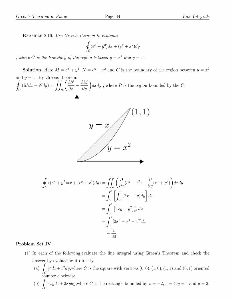
Example 2.16. Use Green’s theorem to evaluate∮C
(ex + y2)dx+ (ey + x2)dy
, where C is the boundary of the region between y = x2 and y = x.
Solution. Here M = ex + y2, N = ey + x2 and C is the boundary of the region between y = x2
and y = x. By Greens theorem:∮C
(Mdx+Ndy) =
∫∫R
(∂N
∂x− ∂M
∂y
)dxdy , where R is the region bounded by the C.
∮C
((ex + y2)dx+ (ey + x2)dy) =
∫∫R
(∂
∂x(ey + x2)− ∂
∂y(ex + y2)
)dxdy
=
∫ 1
0
[∫ x
x2(2x− 2y)dy
]dx
=
∫ 1
0
[2xy − y2
]xx2dx
=
∫ 1
0
[2x3 − x4 − x2]dx
=− 1
30
Problem Set IV
(1) In each of the following,evaluate the line integral using Green’s Theorem and check the
answer by evaluating it directly.
(a)
∫C
y2dx+x2dy,where C is the square with vertices (0, 0), (1, 0), (1, 1) and (0, 1) oriented
counter clockwise.
(b)
∫C
3xydx+2xydy,where C is the rectangle bounded by x = −2, x = 4, y = 1 and y = 2.
44

Line Integrals Page 45 Illustrative Examples
(c)
∫C
(x2 − y)dx+ xdy,where C is the circle x2 + y2 = 4.
(d)
∫C
ln(1 + y)dx− xy
1 + ydy,where C is the triangle with vertices (0, 0), (2, 0) and (0, 4).
(2) Apply Green’s Theorem to evaluate the integral.
∫C
(xy + y2)dx+ x2dy,where C is the
triangle bounded by x = 0.x+ y = 1, y = 0.
(3) Use Green’s Theorem to find the counter clockwise circulation and outward flux of the field
F = xyi + y2j around and over the boundary of the region enclosed by the curves y = x2
and y = x in the first quadrant.
(4) Use Green’s Theorem to find the work done by F = 2xy3i + 4x2y2j in moving a particle
once counter clockwise around the boundary of the triangular region in the first quadrant
enclosed by the x-axis,the line x = 1 and the curve y = x3..
6. Illustrative Examples
(1) Integrate f(x, y, z) = x+√y − z2 over the path from (0, 0, 0) to (1, 1, 1) given by
C1 : r(t) = tk, 0 ≤ t ≤ 1.
C2 : r(t) = tj, 0 ≤ t ≤ 1.
C3 : r(t) = ti, 0 ≤ t ≤ 1.
Solution. Suppose C is the curve joining C1, C2 and C3, as shown in the figure. By Remark
2.2 (Additivity)∫C
f(x, y, z)ds =
∫C1
f(x, y, z)ds+
∫C2
f(x, y, z)ds+
∫C3
f(x, y, z)ds
Along C1 : x = 0, y = 0, z = t, 0 ≤ t ≤ 1
∴∫C
(x, y, z)ds =
∫ 1
0
−t2dt = −1
3Along C2 : x = 0, y = t, z = 1, 0 ≤ t ≤ 1
∴∫C2
f(x, y, z)ds =
∫ 1
0
(√t− 1)dt = −1
3Along C3 : x = t, y = 1, z = 1, 0 ≤ t ≤ 1
∴∫C3
f(x, y, z)ds =
∫ 1
0
t dt =1
2
∴∫C
f(x, y, z)ds = −1
3− 1
3+
1
2= −1
6.
(2) In each part evaluate the integral∫ydx+ zdy − xdz along the stated curve
(a) The line segment from (0, 0, 0) to (1, 1, 1).
(b) The twisted cubic x = t, y − t2, z = t3 from (0, 0, 0) to (1, 1, 1).
(c) The helix x = cosπt, y = sinπt, z = t from (1, 0, 0) to (−1, 0, 1).
Solution.
45

Illustrative Examples Page 46 Line Integrals
(a) Suppose C1 : The line segment from (0, 0, 0) to (1, 1, 1). The equations of the line
passing through (0, 0, 0) to (1, 1, 1) arex
1=y
1=z
1.
∴ C1 : x = t, t = t, z = t, 0 ≤ t ≤ 1.
∴ dx = dt, dy = dt, dz = dt.
∴∫C1
(ydx+ zdy − xdz) =
∫ 1
0
(t+ t− t)dt =1
2.
(b) C2 : x = t, y = t2, z = t3 ∴ dx = dt, dy = 2tdt, dz = 3t2dt.
∴∫C2
(ydx+ zdy − xdz) =
∫ 1
0
(t2 + t3(2t)− t(3t2))dt
=
∫ 1
0
(t2 − 3t2 + 2t4)dt
=− 1
60
(c) C3 : x = cosπt, y = sinπt, z = t ∴ dx = −π sin πtdt, dy = π cos πtdt, dz = dt.
∴∫C3
(ydx+ zdy − xdz) =
∫ 1
0
[(sinπt)(−π sin πt) + t(π cosπt)− (cosπt)]dt
=
∫ 1
0
(−π sin2 πt+ tπ cosπt− cos πt)dt
=
∫ 1
0
(1− cos 2πt)dt
2+ π
[t sin πt
π
]1
0
−∫ 1
0
sin πt−∫ 1
0
cos πtdt
=− π2 + 4
2π.
(3) Find the mass of a thin wire shaped in the form of the curve x = et cos t, y = et sin t, (0 ≤t ≤ 1), if the density function δ is proportional to the distance from the origin.
Solution. Let (x, y) be a point on the thin wire.
Therefore δ ∝√x2 + y2 ∴ δ = k(
√x2 + y2), where k is the constant of the proportionality.
The mass of thin wire is given by
46
Line Integrals Page 47 Illustrative Examples
M =
∫C
δ(x, y)ds
=
∫ 1
0
k1
√(et cos t)2 + (et sin t)2
√(dx
dt
)2
+
(dy
dt
)2
dt
=
∫ 1
0
k√
2et√
2etdt
=
∫ 1
0
k√
2et√
2etdt
=2k
∫ 1
0
e2tdt
=k(e− 1)
(4) Find the centre of mass of a thin wire lying along the curve
r(t) = ti + 2tj +
(2
3
)t3/2k, 0 ≤ t ≤ 2, if the density is δ = 3
√5 + t.
Solution. Suppose C : r(t) = ti + 2tj +
(2
3
)t3/2k
The coordinates of the centre of mass of a thin wire along the curve C whose density is
δ = 3√
5 + t are given by
x =Myz
M,y =
Mxz
M, z =
Mxy
M.
∴M =
∫C
δ(x, y, z)ds
=
∫ 2
0
3√
5 + t√
(1)t2 + (2)t2 + (t2)2dt
=
∫ 2
0
3√
5 + t√
5 + tdt
=3
∫ 2
0
(5 + t)dt
=3[5t+ t2/2]
=36
47

Illustrative Examples Page 48 Line Integrals
Myz =
∫C
xδ(x, y, z)ds
=
∫ 2
0
3t√
5 + t√
1 + 4 + tdt
=
∫ 2
0
3t(5 + t)dt
=
[15
2t2 + t3
]2
0
Myz =38
Mxy =
∫C
yδ(x, y, z)ds
=
∫ 2
0
6t(5 + t)dt
=[15t2 + 2t3
]Mxy =76
Mxy =
∫C
zδ(x, y, z)ds
=
∫ 2
0
2t3/2(5 + t)dt
=
[4t
5/2 +4
7t7/2
]2
0
Mxy =154
7
√2
x =Myz
M,y =
Mxz
M, z =
Mxy
M
x =19
18,y =
19
9, z =
4√
2
7.
(5) Find the work done by the force field F(x, y, z) = (x + y)i + xyj − z2k on a particle that
moves along the line segment from (1, 3, 1) to (2,−1, 4).
Solution. Suppose A(1, 3, 1) and B(2,−1, 4).
d.r.s of AB are 1,−4, 3. Equations of AB arex− 1
1=y − 3
1=z − 1
1Let C : the line segment AB
∴ C : (1 + t)c + (3 + 4t)j + (1 + 3t)k, 0 ≤ t ≤ 1
48

Line Integrals Page 49 Illustrative Examples
The work done by F along C is given by
W =
∫C
F(x, y, z)dr
=
∫ 1
0
[(4− 3t)c + (3− t− 4t2)j− (1 + 3t2)k
]· [i− 4j + 3k] dt
=
∫ 1
0
[1(4− 3t)− 4(3− t− 4t2)− 3(1 + 3t2)
]dt
=
∫ 1
0
(−9t2 − 17t− 11)dt
=
[−3t3 − 17
2− 11t
]1
0
W =45
2
(6) Find the work done by the gradient of f(x, y) = (x+ y2) counter clockwise around the circle
x2 + y2 = 4 from (2, 0) to itself.
Solution. Suppose
F(x, y) = grad f(x, y) =∂f
∂xi +
∂f
∂yj
=2(x+ y)i + 2(x+ y)j
C : Circle x2 + y2 = 4 from (2, 0) to itself.
∴ C : r(t) = 2 cos ti + 2 sin tj, 0 ≤ t ≤ 2π
The work done by F along C is given by
W =
∫C
F(x, y, z)dr
=
∫ 2π
0
[4(cos t+ sin t)i + 4(cos t+ sin t)j] · (−2 sin i + 2 cos j)dt
=8
∫ 2π
0
(cos2 t− sin2 t)dt
=8
∫ 2π
0
cos 2tdt
=8× 0
W =0
(7) Find the flux of the vector field F = (x + y)i − (x2 + y2)j outward across the triangle with
the vertices (1, 0), (0, 1), (−1, 0).
Solution. Suppose P (1, 0), Q(0, 1) and R(−1, 0)
C : 4PQR
49

Illustrative Examples Page 50 Line Integrals
(Flux of F = M i +N j across C) =
∮C
Mdy −Ndx
∴ Flux of F =
∮C
(x+ y)dy + (x2 + y2)dx
=
∫PQ
(x+ y)dy + (x2 + y2)dx+
∫QR
(x+ y)dy + (x2 + y2)dx+∫RP
(x+ y)dy + (x2 + y2)dx.
Along PQ: The equation of PQ is x = 1− y, dx = −dy and 0 ≤ y ≤ 1.
∴∫PQ
(x+ y)dy + (x2 + y2)dx =
∫ 1
0
(2− 2y + 2y2)dy =5
3.
Similarly
∫QR
(x+ y)dy + (x2 + y2)dx = −2
3and
∫RP
= (x+ y)dy + (x2 + y2)dx =2
3.
Hence Flux of F =5
3− 2
3+
2
3=
5
3.
∂N
∂x= z =
∂M
∂y.
F = yzi + xzj + xyk is conservative.
(8) Show that the vector field F = y sin zi + x sin zj + xy cos zk is conservative.
Solution. Here M = y sin z,N = x sin z, P = xy cos z.∂P
∂y= x cos z =
∂N
∂z,∂M
∂z= y cos z =
∂P
∂x,∂N
∂x= sin z =
∂M
∂y.
Hence F is conservative.
(9) Show that the vector field F = yi + (x+ z)j− yk is not conservative.
Solution. Here M = y,N = x+ z, P = −y.∂P
∂y= −1 ,
∂N
∂z= 1,
∂M
∂z= 0
∂P
∂y6= ∂N
∂z.F is not conservative.
(10) Find a potential function f for the field F.
Solution. Comparing F=(y + z)i + (x+ z)j + (x+ y)k with F= M i +N j + Pk we have
M = y + z,N = x+ z, P = x+ y∂P
∂y= 1 =
∂N
∂z,∂M
∂z= 1 =
∂P
∂x,∂N
∂x= 1 =
∂M
∂yBy Remark 2.9 F is conservative and we can find a potential function f by integrating the
equations∂f
∂x= y + z,
∂f
∂y= x+ z,
∂f
∂z= x+ y
We integrating the first equation with respect to x,keeping y and z constant.
f(x, y, z) = x(y + z) + g(y, z)
We write the constant of integration as a function of y and z.Now we can find∂f
∂yfrom this
equation and equate it with the expression∂f
∂y.
50
Line Integrals Page 51 Illustrative Examples
x+∂g
∂y= x+ z
From the last equation we get,∂g
∂y= z.Therefore g = yz + h(z) .
f(x, y, z) = x(y + z) + yz + h(z)
We now calculate∂f
∂zfrom this equation and
equate it to the expression∂f
∂z.
x+ y +dh
dz= x+ y.It gives
dh
dz= 0.So h(z) = k
Hence f(x, y, z) = xy + xz + yz + k.
(11) Find the work done by
F = eyzi + (xzeyz + z cos y)j + (xyeyz + sin y)k over the following paths from (1, 0, 1) to
(1, π/2, 0)
a. The line segment:x = 1, y = πt/2, z = 1− t ,0 ≤ t ≤ 1.
b. The line segment from (1, 0, 1) to the origin followed by the line segment from the origin
to (1, π/2, 0).
c. The line segment from (1, 0, 1) to (1, 0, 0) followed by the x−axis from (1, 0, 0) to the
origin,followed by the parabola y =πx2
2, z = 2 from there to (1, π/2, 0).
Solution. Comparing F = eyzi+(xzeyz+z cos y)j+(xyeyz+sin y)k with F= M i+N j+Pk
we have
M = eyz, N = xzeyz + z cos y, P = xyeyz + sin y∂P
∂y= xeyz(yz + 1) + cos y =
∂N
∂z,∂M
∂z= yeyz =
∂P
∂x,∂N
∂x= zeyz =
∂M
∂yBy Remark 2.9 F is conservative.Hence the work done by
F =
∫C
F · dr is independent of the path.
Also
∫C
F · dr = f(1, π/2, 0)−f(1, 0, 1),where F = ∇f . Now we can find a potential function
f by integrating the equations∂f
∂x= eyz,
∂f
∂y= xzeyz + z cos y,
∂f
∂z= xyeyz + sin y
We integrating the first equation with respect to x,keeping y and z constant.
f(x, y, z) = xeyz + g(y, z)
We write the constant of integration as a function of y and z.Now we can find∂f
∂yfrom this
equation and equate it with the expression∂f
∂y.
xzeyz +∂g
∂y= xzeyz + z cos y
From the last equation we get,∂g
∂y= z cos y.Therefore g = z sin y + h(z) .
51

Illustrative Examples Page 52 Line Integrals
f(x, y, z) = xeyz + z sin y + h(z)
We now calculate∂f
∂zfrom this equation and
equate it to the expression∂f
∂z.
xyeyz + sin y +dh
dz= xyeyz + sin y.It gives
dh
dz= 0.So h(z) = k
Hence f(x, y, z) = xeyz + z sin y + k.f(1, π/2, 0) = 1 + k, f(1, 0, 1) = 1 + k∫C
F · dr = f(1, π/2, 0)− f(1, 0, 1) = 0
The work done by F along each path is 0.
(12) Show that the integral∫C
(yzdx+ xzdy + yx2)
is not independent of the path.
Solution. It is sufficient to show that F = yzi + xzj + yx2k is not conservative. Here
M = yz,N = xz, P = yx2.∂P
∂y= x2 ,
∂N
∂z= x,
∂M
∂z= y
∂P
∂y6= ∂N
∂z.F is not conservative.Hence the given integral is not independent of the path.
(13) Use Green’s theorem to evaluate the integral
∮C
y tan2 xdx+ tanxdy
,
where C is the circle x2 + (y + 1)2 = 1
Solution. Here M = y tan2 x, N = tanx and C is the boundary of the region between
y = x2 and y = x. By Greens theorem:∮C
(Mdx+Ndy) =
∫∫R
(∂N
∂x− ∂M
∂y
)dxdy , where R is the region bounded by the C.∮
C
(y tan2 xdx+ tanxdy) =
∫∫R
(∂
∂xtanx− ∂
∂yy tan2 x
)dxdy
=
∫∫R
(sec2 x− tan2 x)dxdy
=
∫∫R
1dxdy
=area of the circle
=π
(14) Use Green’s theorem to evaluate the integral∮C
cosx sin ydx+ sinx cos ydy,
where C is the triangle with vertices (0, 0), (3, 3), (0, 3)
52

Line Integrals Page 53 Illustrative Examples
Solution. Here M = cosx sin y, N = sinx cos y. By Greens theorem:∮C
(Mdx+Ndy) =
∫∫R
(∂N
∂x− ∂M
∂y
)dxdy , where R is the region bounded by the C.∮
C
(cosx sin ydx+ sinx cos ydy) =
∫∫R
(∂
∂xsinx cos y − ∂
∂ycosx sin y
)dxdy
=
∫∫R
cosx cos y − cosx cos ydxdy
=0
(15) Use Green’s theorem to find the work done by the force F = xyi + (x2
2+ xy)j, the particle
starts at (5, 0),transverse the upper semi circle x2 + y2 = 25 and returns to its starting point
along the x−axis.
Solution. The work done by the force F is∫C
F · dr =
∮C
Mdx+Ndy,
where M = xy, N = (x2
2+ xy). By Greens theorem:∮
C
(Mdx+Ndy) =
∫∫R
(∂N
∂x− ∂M
∂y
)dxdy , where R is the region bounded by the C.
∮C
(xydx+ (x2
2+ xy)dy) =
∫∫R
(∂
∂x(x2
2+ xy)− ∂
∂yxy
)dxdy
=
∫ 5
−5
(∫ √25−x2
0
ydy
)dx
=
∫ 5
−5
[y2/2
]√25−x2
0dx
=
∫ 5
0
(25− x2)dx
=250
3
(16) Using Green’s theorem,show that the area bounded by a simple closed curve Cis given by1
2
∮C
xdy − ydx.
Hence find the area of the ellipse x2/9 + y2/4 = 1
53

Illustrative Examples Page 54 Line Integrals
Solution. Suppose M = −y,N = x.If R is the region bounded by a simple closed curve
C,then by Green’s theorem we have∮C
(Mdx+Ndy) =
∫∫R
(∂N
∂x− ∂M
∂y
)dxdy
∮C
xdy − ydx =
∫∫R
(∂
∂xx− ∂
∂y(−y)
)dxdy
=
∫∫R
(1 + 1)dxdy
=
∫∫R
2dxdy
=2(area of the regionR)
Hence the area of the region R=1
2
∮C
xdy − ydx
Now we find the area of the ellipse C : x2/9+y2/4 = 1.C : x = 3 cos t, y = 2 sin t; 0 ≤ t ≤ 2π.
area of the ellipse =1
2
∮C
xdy − ydx
=1
2
∫ 2π
0
6 cos2 t+ 6 sin2 tdt
=1
2
∫ 2π
0
6dt
=3π
(17) Evaluate the integral∫C
(e−x + 3y)i + xj · dr
C is the boundary of the region R between the circles x2 + y2 = 16 and x2− 2x+ y2 = 3 and
C is oriented so that the region is on the left when the boundary transverse in the direction
of its orientation.
Solution. Here M = e−x + 3y and N = x.C is the simple closed curve.By Green’s theorem
54

Line Integrals Page 55 Illustrative Examples
∫C
(e−x + 3y)i + xj · dr =
∫∫R
(∂
∂xx− ∂
∂y(e−x + 3y)
)dxdy
=
∫∫R
(1− 3)dxdy
=
∫∫R
(−2)dxdy
=− 2[area of the circle (x2 + y2 = 16)− area of the circle (x2 − 2x+ y2 = 3)]
=− 2(16π − 4π)
=− 24π
55

Exercise Page 56 Line Integrals
7. Exercise
(1) In each part,evaluate the integral∫C
(3x+2y)dx+(2x-y)dy along the stated curves
(a) The line segment from (0, 0) to (1, 1).
(b) The parabolic arc y = x2 from (0, 0) to (1, 1).
(c) The curve y = sin(πx/2) from (0, 0) to (1, 1).
(d) The curve y = x3 from (0, 0) to (1, 1).
(2) Evaluate the line integral∫C
3x2yz ds where C : x = t, y = t2, z =2
3t3.
(3) Evaluate the line integral∫C
(x+y)ds where C is the line segment from (0, 1, 0) to (1, 0, 0).
(4) Integrate f(x, y, z) = (x+ y + z)/(x2 + y2 + z2) over the path
r(t)= ti + tj + tk, 0 ≤ t ≤ 1.
(5) Integrate f(x, y) = x+ y over the curve C : x2 + y2 = 4 in the first quadrant form (2, 0) to
(0, 2).
(6) Find the mass of a thin wire shaped in the form of the helix x = 3 cos t, y = 3 sin t, z = 4t
(0 ≤ t ≤ π/2) if the density function is δ = kx/(1 + y2) k > 0.
(7) Find the mass of a wire that lies along the curve r(t)= (t2 − 1)j + 2tk,
0 ≤ t ≤ 1,if the density is δ = (3/2)t.
(8) Find the centre of mass of a thin wire lying along the curve r(t)= ti+(2√
2/3)t3/2j+t2/2k, 0 ≤t ≤ 2 if the density is δ = 1/(t+ 1).
(9) Find the work done by the force field F(x,y,z)= xyi + yzj + xzk on a particle that moves
along the curve C:r(t)= ti + t2j + t3k, (0 ≤ t ≤ 1).
(10) Suppose that a particle moves through the force field F(x,y)= xyi + (x− y)j from the point
(0, 0) to the (1, 0) along the curve x = t, y = λt(1 − t).For what values of λ will the work
done by the force field be 1?
(11) Find the circulation and flux of the vector fields F(x,y)= −yi + xj around and the closed
semicircular path that consists of the semicircular arch r1(t)= a cos ti + a sin tj, (0 ≤ t ≤ π)
followed by the line segment r2(t)= ti,−a ≤ t ≤ a.
(12) Find the flow of the velocity field F=(x+ y)i− (x2 + y2)j along each of the following paths
from (1, 0) to (−1, 0).
(a) The upper half of the circle x2 + y2 = 1.
(b) The line segment from (1, 0) to (−1, 0).
56

Line Integrals Page 57 Exercise
(c) The line segment from (1, 0) to (0,−1) followed by the line segment from (0,−1) to
(−1, 0).
(13) The field F = xyi + yj − yzk is the velocity field of a flow in space. Find the flow from
(0, 0, 0) to (1, 1, 1) along the curve of intersection of the cylinder y = x2 and the plane z = x.
(14) Show that the line integral∫C
y2dx + 2xydy is independent of the path.Also evaluate the line integral along the line
segment from (−1, 2) to (1, 3).
(15) Show that each of the following integral is independent of the path,and use Remark 2.8 to
find its value.
(a)
∫ (4,0)
(1,2)
3ydx+ 3xdy.
(b)
∫ (3,2)
(0,0)
2xeydx+ x2eydy.
(c)
∫ (−1,0)
(2,−2)
2xy3dx+ 3y2x2dy.
(16) In each of the following find a potential function f for the vector field F
(a) F = 2xi + 3yj + 4zk.
(b) F = ey+2z(i + xj + 2xk).
(c) F = (lnx+ sec2(x+ y))i +
(sec2(x+ y) +
y
y2 + z2
)j +
z
y2 + z2k.
(17) Find a potential function for F =2x
yi +
(1− x2
y2
)j[x2 − 1
y]
(18) Find the work done by F = (x2 +y)i+(y2 +x)j+zezk over the following paths from (1, 0, 0)
to (1, 0, 1).
(a) The line segment x = 1, y = 0, 0 ≤ z ≤ 1.
(b) The helix r(t) = cos ti + sin tj +t
2πk, 0 ≤ t ≤ 2π
(c) The x-axis from (1, 0, 0) to (0, 0, 0) followed by the parabola z = x2, y = 0 from (0, 0, 0)
to (1, 0, 1).
(19) In each of the following,evaluate the line integral using Green’s Theorem and check the
answer by evaluating it directly.
(a)
∫C
x cos ydx − y sinxdy,where C is the square with vertices (0, 0), (π/2, 0), (π/2, π/2)
and (0, π/2).
(b)
∫C
tan−1 ydx− y2x
1 + y2dy,where C is the square with vertices (0, 0), (1, 0), (1, 1) and (0, 1).
(c)
∫C
x2ydx+ (y + xy2)dy,where C is the boundary of the region enclosed by y = x2 and
x = y2.
57

Exercise Page 58 Line Integrals
(20) Use Green’s Theorem to find the work done by the force field F(x, y) = xyi + (1
2x2 + xy)j;
the particle starts at (5, 0),transverse the upper semicircle x2 + y2 = 25 and returns to its
starting point along the x-axis.
(21) Find a simple closed curve C with counter clockwise orientation that maximizes the value
of∫C
1
3y3dx+ (x− 1
3x3)dy and explain your reasoning.
(22) (a) Let C be the line segment from a point (a, b) to a point (c, d).Show that∫C
−ydx+ xdy= ad− bc.
(b) Use the result in part (a) to show that the area A of a triangle with successive vertices
(x1, y1), (x2, y2) and (x3, y3) going counter clockwise is
A = [(x1y2 − x2y1) + (x2y3 − x3y2) + (x3y1 − x1y3)].
(23) Find a formula for the area of a polygon with successive vertices (x1, y1), (x2, y2) . . . (xn, yn)
going counter clockwise.
(24) Evaluate the integral
∫C
[(x2 + y)i + (4x − cos y)j] · dr; C is the boundary of the region R
that is inside the square with vertices (0, 0), (5, 0), (5, 5) and (0, 5) but outside the rectangle
with vertices (1, 1), (3, 1), (3, 2), (1, 2) and C is oriented so that the region is on the left when
the boundary is traversed in the direction of its orientation.
(25) In each of the following,use Green’s Theorem to find the counter clockwise circulation and
outward flux for the field F and curve C.
(a) F = (x− y)i + (y − x)j;C : the square bounded by x = 0, x = 1, y = 0, y = 1.
(b) F = (y2 − x2)i + (x2 + y2)j;C : the triangle bounded by x = 3, y = 0, y = x.
(26) Apply Green’s Theorem to evaluate the integral
∫C
(6y + x)dx+ (y + 2x)dy,where C is the
circle (x− 2)2 + (y − 3)2 = 4.
58

Line Integrals Page 59 Answers
8. Answers
8.1. Problem Set I. (1)1
12(17√
17− 1), (2) −15
32(e14− e16), (3) 6
√3, (4)
15
2, (5)
2
3(5√
5− 1),
(7) 0, (8) 0.
8.2. Problem Set II. (1)3
5, (2) (a) circ1 = 0 circ2 = 2π flux1 = 2π flux2 = 0 (b) circ1 = 0
circ2 = 8π flux1 = 7π flux2 = 0, (3) (a)1
2(b) −π.
8.3. Problem Set III. (1) (a)−2x
x2 + y2i− −2y
x2 + y2j+exk (b)
2x√x2 + y2 + z2
i+2y√
x2 + y2 + z2j+
2z√x2 + y2 + z2
k (c) (y + z)i + (x + z)j + (x + y)k, (2) (a) conservative,x2/2 + y2/2 + k (b) non
conservative (c) conservative x cos y + y sin z + k, (3) (a) 49 (b) -16 (c) 1
8.4. Exercise. (1) (a) 3 (b) 3 (c) 3, (2) 13/2, (3)√
2, (4)√
3 log b/a, (5) 8, (6) 5k tan−1 3, (7)
4√
2− 2, (9) 27/28,
(10) λ = −12, (11) circ = a2 π flux= 0, (12) (a) − π/2 (b) 0 (c) 1, (13) 1/2, (14) 13,
(15) (a) −6 (b) 9e2 (c) 32, (16) (a) f(x, y, z) = x2 + 3y2/2 (b) f(x, y, z) = xey+2z + k (c) f(x, y, z) =
x lnx − x + tan(x + y) + (1/2) ln(y2 + z2) + k, (17) x2 − 1/y, (18) (a) 1 (b) 1 (c) 1, (19) (a) 0 (b) -1
(0), (20) 250/3, (21) x2 + y2 = 1, (24) 69, (25) (a) circ= 0, flux= 2 (b) circ = 0 flux -9, (26) −16π
59


CHAPTER 3
Surface and Volume Integrals
Introduction
In the last Chapter, we have seen how to integrate a function over a flat region in a plane. Here
question arises that how to integrate, if the function is defined over a curved surface? That is given
by double integral over a region in a co-ordinate plane.
1. Surface Area and Surface integrals
Surface Area
The surface is defined by the equation f(x, y, z) = C If the surface is smooth, then we can define
and calculate its area as a double integral over region R.
Suppose S is a surface of area, we take the partition of region R into small rectangles ∆Ak. The upper
partition of ∆Ak is ∆σk which may be approximate tangent plane to the partition ∆Pk. We suppose
that ∆Pk is a portion of the plane that is tangent to the surface at that point Tk(xk, yk, zk), which is
upper portion of corner Ck of ∆Ak. If the tangent plane is parallel to R, then ∆Pk will be congruent
to ∆Ak. Let ∆f(xk, yk, zk)k be the gradient at Tk(xk, yk, zk) and a unit vector P that is normal to R.
The angle between ∆f and P is γk. Let uk and vk be the vectors along the edges of portion ∆Pk in
the tangent plane. Thus uk×vk and ∆f both are normal to the tangent plane. Therefore|uk × vk · P |gives the area of the projection of the parallelogram determine by uk and vk onto any plane whose
normal is P . ⇒ |uk × vk.P | = ∆Ak . . . (1) Now, |uk × vk| itself is the area ∆Pk [ by properties of
cross product] so the equation (1) becomes |uk × vk| |P | |cos(angle betweenuk × vkandP )| = ∆Ak (by
definition of dot product) . . . (2) or ∆Pk |cos γk| = ∆Ak.
or ∆Pk =∆Ak|cos γk|
provides cos γk 6= 0. We will have cos γk 6= 0 as long as ∇f is not parallel to the
ground plane and ∇f · P 6= 0 Since the portion ∆Pk approximate the surface portion ∆σk that fit
together to make S, the sum∑
∆Pk =∑ ∆Ak|cos γk|
. . . (3) The sums on the right-hand side of equation
(3) are approximating sums for the double integral
∫∫R
1
cos γdA . . . (4) which gives the area of S to
be the value of this integral whenever it exists that is, for any surface f(x, y, z) = c
We have |∇f · P | = |∇f | |P | |cos γ|,
61

Surface Area and Surface integrals Page 62 Surface and Volume Integrals
So1
cos γ=|∇f ||∇f · P |
Which is equivalent to equation (4)
Therefore the area of the surface f(x, y, z) = c over a closed and bounded plane region R is
surface area =
∫∫R
∇f∇f · P
dA . . . (5),
where P is a unit vector normal to R and ∇f · P 6= 0.
Thus, the area is the double integral over R of the magnitude of ∇f divided by the magnitude of
the scalar component of ∇f normal to R.
We reduced equation (5) under the assumption that ∇f ·P 6= 0 throughout R and ∇f is continuous.
Whenever the integral exists, however, we define its values to be the area of the portion of the surface
f(x, y, z) = c that lies over R.
Example 3.1. Find the area of the surface cut from the bottom of the paraboloid x2 + y2− z = 0
by the plane z = 4.
Solution. The surface S is part of the level surface f(x, y, z) = x2 + y2 − z = 0, and R is the
disk x2 + y2 ≤ 4 in the xy-plane. We take a unit vector normal to the plane of R, is P = k
We have f(x, y, z) = x2 + y2 − z∇f = 2xi+ 2yj − k∴ |∇f | =
√(2x)2 + (2y)2 + (−1)2
62
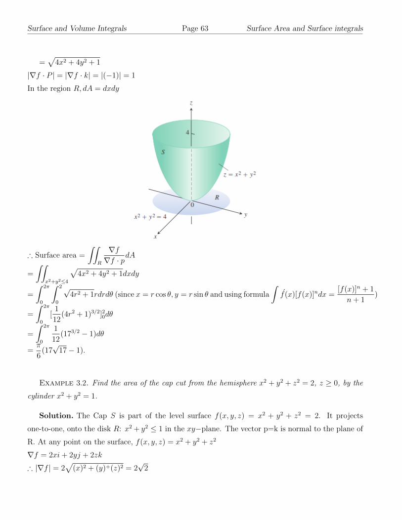
Surface and Volume Integrals Page 63 Surface Area and Surface integrals
=√
4x2 + 4y2 + 1
|∇f · P | = |∇f · k| = |(−1)| = 1
In the region R, dA = dxdy
∴ Surface area =
∫∫R
∇f∇f · p
dA
=
∫∫x2+y2≤4
√4x2 + 4y2 + 1dxdy
=
∫ 2π
0
∫ 2
0
√4r2 + 1rdrdθ (since x = r cos θ, y = r sin θ and using formula
∫f(x)[f(x)]ndx =
[f(x)]n + 1
n+ 1)
=
∫ 2π
0
[1
12(4r2 + 1)3/2]20dθ
=
∫ 2π
0
1
12(173/2 − 1)dθ
=π
6(17√
17− 1).
Example 3.2. Find the area of the cap cut from the hemisphere x2 + y2 + z2 = 2, z ≥ 0, by the
cylinder x2 + y2 = 1.
Solution. The Cap S is part of the level surface f(x, y, z) = x2 + y2 + z2 = 2. It projects
one-to-one, onto the disk R: x2 + y2 ≤ 1 in the xy−plane. The vector p=k is normal to the plane of
R. At any point on the surface, f(x, y, z) = x2 + y2 + z2
∇f = 2xi+ 2yj + 2zk
∴ |∇f | = 2√
(x)2 + (y)+(z)2 = 2√
2
63

Surface Area and Surface integrals Page 64 Surface and Volume Integrals
|∇f · p| = |∇f · k| = |(2z)| = 2z
∴ Surface area =
∫∫R
|∇f ||∇f · p|
dA
=
∫∫R
2√
2
2zdA =
√2
∫∫R
dA
zNow x2 + y2 + z2 = 2
∴ z =√
2− x2 − y2
∴ surface area =√
2
∫∫R
dA
z=√
2
∫∫x2+y2≤1
dA√2− x2 − y2
=√
2
∫ 2π
0
∫ 1
0
[rdrdθ√2− r2
=√
2
∫ 2π
0
[−(2− r2)1/2]r=1r=0dθ
=√
2
∫ 2π
0
(√
2− 1)dθ.
= 2π(2−√
2)
64

Surface and Volume Integrals Page 65 Surface Area and Surface integrals
Surface integrals
Now we see how to integrate a function over a surface,using the idea of surface area.
Definition 3.1. (Surface Integral):Let R be the shadow region on the ground plane of a surface
S defined by the equation f(x, y, z) = c. If g is a continuous function defined on S,then the integral
of g over S is the integral∫∫R
g(x, y, z)∇f|∇f · p|
dA,
where p is a unit normal to R and ∇f · p 6= 0.
This integral is called the surface integral.
Orientation:We say that a smooth surface S is orientable or two-sided if it is possible to define
a field n of unit normal vectors on S that varies continuously with position.
Spheres and other smooth closed surfaces in space are orientable.The Mobius band is not orientable.
Definition 3.2. (Surface Integral for Flux):The flux of a three-dimensional vector field F across
an oriented surface S in the direction of n is given by
Flux=
∫∫R
F · ndσ
If S is a part of a level surface g(x, y, z) = c,then n may be taken to be one of the two fields
n = ± ∇g|∇g|
Remark1:If we take the projection R of S on xy−plane then∣∣n · k∣∣ ds = dxdy
therefore
∫∫S
F · nds =
∫∫R
F · ndxdyn · k
Remark2 If we take the projection R of S on xz−plane then |n · j| ds = dxdz
therefore
∫∫S
F · nds =
∫∫R
F · ndxdzn · j
Remark3 If we take the projection R of S on yz−plane then |n−.i−| ds = dydz
therefore
∫∫S
F · nds =
∫∫R
F · ndydzn · i
Moments and Masses of Thin Shells:
Thin shells of material like bowls metal drums, and domes are modeled with surfaces. Their moments
and masses are calculated with the formulas, given below
M =
∫∫S
δ(x, y, z)dσ, where δ(x, y, z) = density at (x, y, z), mass per unit area.
First moments about the coordinate planes;
Myz =
∫∫S
xδdσ,Mxz =
∫∫S
yδdσ,Mxy =
∫∫S
zδdσ,.
Coordinates of center of mass:
x =Myz
M, y =
Mxz
M, z =
Mxy
M
65
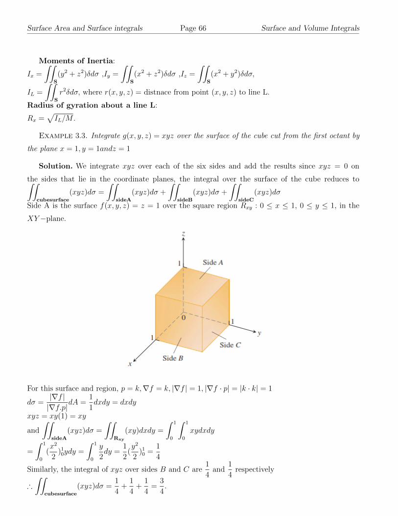
Surface Area and Surface integrals Page 66 Surface and Volume Integrals
Moments of Inertia:
Ix =
∫∫S
(y2 + z2)δdσ ,Iy =
∫∫S
(x2 + z2)δdσ ,Iz =
∫∫S
(x2 + y2)δdσ,
IL =
∫∫S
r2δdσ, where r(x, y, z) = distnace from point (x, y, z) to line L.
Radius of gyration about a line L:
Rx =√IL/M .
Example 3.3. Integrate g(x, y, z) = xyz over the surface of the cube cut from the first octant by
the plane x = 1, y = 1andz = 1
Solution. We integrate xyz over each of the six sides and add the results since xyz = 0 on
the sides that lie in the coordinate planes, the integral over the surface of the cube reduces to∫∫cubesurface
(xyz)dσ =
∫∫sideA
(xyz)dσ +
∫∫sideB
(xyz)dσ +
∫∫sideC
(xyz)dσ
Side A is the surface f(x, y, z) = z = 1 over the square region Rxy : 0 ≤ x ≤ 1, 0 ≤ y ≤ 1, in the
XY−plane.
For this surface and region, p = k,∇f = k, |∇f | = 1, |∇f · p| = |k · k| = 1
dσ =|∇f ||∇f.p|
dA =1
1dxdy = dxdy
xyz = xy(1) = xy
and
∫∫sideA
(xyz)dσ =
∫∫Rxy
(xy)dxdy =
∫ 1
0
∫ 1
0
xydxdy
=
∫ 1
0
(x2
2)10ydy =
∫ 1
0
y
2dy =
1
2(y2
2)10 =
1
4
Similarly, the integral of xyz over sides B and C are1
4and
1
4respectively
∴∫∫
cubesurface
(xyz)dσ =1
4+
1
4+
1
4=
3
4.
66
Surface and Volume Integrals Page 67 Surface Area and Surface integrals
Example 3.4. Evaluate
∫∫S
F·nds over the entire surface S of the region bounded by the cylinder
x2 + z2 = 9, x = 0, y = 0, z = 0 and y = 8, if F = 6zi+ (2x+ y)j − xk
Solution. Since we have to evaluate
∫∫over the entire surface hence we have divide it into
three parts lower and upper circular path and curved part of height clearly surface area of lower
circle is 9π and that of upper circle is 9π.
∴ Total area of circle is 18π . . . (1)
Let us take the projection R on xy−plane.
∴∫∫
S
F · nds =
∫∫F · n∣∣n · k∣∣dxdy . . . (2)
∴ n =∇s|∇s|
=2xi+ 2zk√4x2 + 4z2
=xi+ zk
3n · k =
z
3
F · n = [6zi+ (2x+ y)j − xk] · xi+ zk
3
=1
3(6xz − xz) =
5xz
3
∴F · n∣∣n · k∣∣ =
5xz
3× 1
z/3= 5x.∫∫
F · n∣∣n · k∣∣dxdy =
∫ x=3
x=−3
∫ y=8
y=0
5xdxdy
=
∫ x=3
x=−3
[5xy]80dx = 40
∫ 3
−3
xdx
= 40
(x2
2
)3
−3
= 40(9/2− 9/2) = 0
∴ Required double integral from (1) and (2)∫∫SF · nds = 18π.
Example 3.5. Evaluate
∫∫S
F · nds where F = zi+xj− 3y2zk and S the surface of the cylinder
x2 + y2 = 16 included in the first octant between z = 0 and z = 5.
Solution. Let us take the projection R of S on yz−plane
∴∫∫
S
F · nds =
∫∫R
F · n dydz|n · i|
n =∇s|∇s|
=2xi+ 2yj√4x2 + 4y2
=xi+ yj
4
67

Surface Area and Surface integrals Page 68 Surface and Volume Integrals
n · i =x
4
F · n = [zi+ xj − 3y2zk] · xi+ yj
4
=1
4(xz + xy) =
5xz
3
∴F · n|n · i|
=1
4× xz + xy
x/4= y + z.∫∫
R
F · n|n · i|
dydz =
∫ y=4
y=0
∫ z=5
z=0
(y + z)dzdy ( by putting x = 0 in x2 + y2 = 16 so y = ±4 )
=
∫ 4
0
[yz +z2
2]50dx =
∫ 4
0
(5y +25
2)dy
=
(5y2
2+
25y
2
)4
0
= 40 + 50 = 90
Example 3.6. Calculate flux of F where F = xi+ yj + 2zk over the surface x2 + y2 + z2 = a2.
Solution. Since we have calculate flux over the entire surface but entire surface is 8 time the
surface in first octant
∴∫∫
S
F · nds =
∫∫S
F · nds. . . (1)
where S is surface in first octant. Let us consider the projection of R of S on XY plane.
∴∫∫
S
F · nds =
∫∫R
F · n∣∣n · k∣∣dxdyNow n =
∇s|∇s|
=2xi+ 2yj + 2zk√
4x2 + 4y2 + 4z2
∴ n =xi+ yj + zk
an · k =
z
a
F · n =x2 + y2 + 2z2
a
∴F · n∣∣n · k∣∣ =
x2 + y2 + 2z2
z.∫∫
R
F · n∣∣n.k∣∣dxdy =
∫∫R
x2 + y2 + 2z2
zdxdy
=
∫∫R
x2 + y2 + 2(a2 − x2 − y2)√a2 − x2 − y2
dxdy
We have to find double integral over R, integrate over an elementary strip parallel over an elementary
srtip parallel to Y-axis from y = 0 to y =√a2 − x2
(Since plane is XY, so z = 0)
Again keeping x fixed and then move the strip from x = 0 to x = a (on X-axis, y = 0 and z = 0)∫ x=a
x=0
∫ y=√a2−x2
y=0
2a2 − x2 − y2√a2 − x2 − y2
dxdy
68

Surface and Volume Integrals Page 69 Surface Area and Surface integrals
=
∫ x=a
x=0
∫ y=√a2−x2
y=0
√a2 − x2 − y2dxdy +
∫ x=a
x=0
∫ y=√a2−x2
y=0
a2√a2 − x2 − y2
dxdy
=
∫ x=a
x=0
[y
2
√a2 − x2 − y2 +
a2 − x2
2sin−1 y√
a2 − x2
]dx+ a2
∫ a
0
[sin−1 y√
a2 − x2
]√a2−x20
dx
=
∫ a
0
π
2
(a2 − x2)
2dx+ a2
∫ a
0
π
2dx
=π
4
∫ a
0
[a2 − x2]dx+πa2
2
∫ a
0
dx
=π
4[a2x− x3
3]a0 +
πa2
2[x]a0
=π
4[a3 − a3
3] +
πa3
2
=π8
12a3 =
π2a3
3
∴∫∫
S
F.nds =π8
12a3 =
π2a3
3
∴ by (1)
∫∫S
F · nds =π16
3a3 .
Example 3.7. Find the center of mass of a thin hemispherical shell of radius a and constant
density δ.
Solution. We model the shell with the hemisphere f(x, y, z) = x2 + y2 + z2 = a2, z ≥ 0.
The symmetry of the surface abput the Z-axis tells us that x = y = 0. It remains only to find z from
the formula z = Mxy/M .
The mass of the shell is M =
∫∫S
δ(x, y, z)dσ
= δ
∫∫S
dσ = δ(areaofS)
= δ(2πa2)
69

Surface Integral for parametrized surface Page 70 Surface and Volume Integrals
= 2πa2δ.
To evaluate the integral for Mxy we take p=k and calculate
|∇f | = |2xi+ 2yj + 2zk| = 2√x2 + y2 + z2 = 2a
|∇f · p| = |∇f · k| = |2z| = 2z
dσ =|∇f | dA|∇f.k|
=2a
2zdA =
a
zdA
Then using the formula for Mxy =
∫∫S
zδdσ
= δ
∫∫S
z × a
zdA = δa
∫∫S
dA = δa(πa2) = πδa3
∴ Using z =Mxy
M=
πδa3
2πa2δ=a
2∴ The Shell’s center of mass is the point (0, 0, a/2).
Problem Set I
(1) Find the area of the band cut from the paraboloid x2 + y2 − z = 0 by the plane z = 6.
(2) Find the area of the region cut from the plane X + 2y + 2z = 5 by the cylinder where wells
are x = y2 and x = 2− y2.
(3) Integrate g(x, y, z) = (xyz) over the surface of the rectangular solid cut from the first octant
by the planes x = a, y = b and z = c.
(4) Integrate g(x, y, z) = x+ y + z over the surface of the cube cut from the first octant by the
planes x = a, y = a, z = a.
(5) Evaluate
∫∫S
F.nds where F = (x + y2)i + 2xj + 2yzk and S is the part of the plane
2x+ y + 2z = 6 in the first octant.
(6) If F = 4xzi− y2j + yzk, evaluate
∫∫S
F.nds where S is the surface of the cube bounded by
x = 0, x = 1, y = 0, y = 1, z = 0, z = 1.
(7) Calculate the Flux of F where F = −i + 2j + 3k and S is the part of rectangular surface
z = 0, 0 ≤ x ≤ 2, 0 ≤ y ≤ 3 by taking projection xy−plane.
(8) Calculate the Flux of F where F = xi + yj + 3k over the surface x2 + y2 + z2 = a2 in the
first octant.
2. Surface Integral for parametrized surface
Parametrization of Surface
We know that the equations of the form z = f(x, y)(explicit form) and F (x, y, z) = 0(implicit form)
represent surfaces in space.
There is also a parametric form of a surface,which can be expressed in terms of two parameters. Let
r(u, v) = f(u, v)i+ g(u, v)j + h(u, v)k. . . (1)
70

Surface and Volume Integrals Page 71 Surface Integral for parametrized surface
be the continuous vector function that is defined on a region R in the uv−plane and one-to-one
on the interior of R. We call the range of r the surface S.The equation (1) together with the
domain R represent a parametrization of the surface. The variables u and v are the parameters,
and R is parameter domain.The equation (1) is the vector equivalent of three parametric equations:
x = f(u, v), y = g(u, v), z = h(u, v)
A parametrized surface r(u, v) = f(u, v)i + g(u, v)j + h(u, v)k is smooth if ru =∂r
∂uand rv =
∂r
∂v
are continuous; and∂r
∂u× ∂r
∂vis never zero on the parameter domain.
The area of a smooth surface r(u, v) = f(u, v)i+ g(u, v)j+h(u, v)k;a ≤ u ≤ b, c ≤ v ≤ d is given by
A =
∫ d
c
∫ b
a
|ru × rv|dudvSurface Integral Using the Parametrized form
If S is a smooth surface defined parametrically as r(u, v) = f(u, v)i + g(u, v)j + h(u, v)k, a ≤ u ≤b, c ≤ v ≤ d and G(x, y, z) is a continuous function defined on S, then the integral of G over S is∫∫
S
G(x, y, z)dσ =
∫ d
c
∫ b
a
G (f(u, v), g(u, v), h(u, v)) |ru × rv| dudv.
Example 3.8. Find a parametrization of the cone z =√x2 + y2, 0 ≤ z ≤ 1.
Solution. Here cylindrical co-ordinates provide everything we need, a point (x, y, z) on the cone
has x = r cos θ, y = r sin θ and z =√x2 + y2 = r with 0 ≤ z ≤ 1 and 0 ≤ θ ≤ 2π.
Taking u = r, v = θ in the equation r(u, v) = f(u, v)i + g(u, v)j + h(u, v)k r(r, θ)=(r cos θ)i +
(r sin θ)j + rk
0 ≤ r ≤ 1, 0 ≤ θ ≤ 2π.
This is required parametrization.
Example 3.9. Find a parametrization of the paraboloid z = x2 + y2, z ≤ 4.
71

Surface Integral for parametrized surface Page 72 Surface and Volume Integrals
Solution. In cylindrical co-ordinates, a point (x, y, z) has x = r cos θ, y = r sin θ, z = z
For points on the paraboloid : z = x2 + y2, x = r cos θ, y = r sin θ, z = r2 0 ≤ r ≤ 2, 0 ≤ θ ≤ 2π
Taking u = r and v = θ.
r(r, θ)=(r cos θ)i+ (r sin θ)j + r2k
0 ≤ r ≤ 2, 0 ≤ θ ≤ 2π.
This is required parametrization.
Example 3.10. Find a parametization of the sphere x2 + y2 + z2 = a2.
Solution. In spherical co-ordinate, point (x, y, z) has x = a sinφ cos θ, y = a sinφ sin θ and
z = a cosφ with 0 ≤ φ ≤ π and 0 ≤ θ ≤ 2π.
Taking u = φ and v = θ in equation r(u, v) = f(u, v)i+ g(u, v)j + h(u, v)k r(φ, θ)=(a sinφ cos θ)i+
(a sinφ sin θ)j + a cosφk
Which gives the required parametrization.
Example 3.11. Find a parametization of the cylinder x2 + (y − 3)2 = 9, 0 ≤ z ≤ 5.
Solution. In cylindrical co-ordinate, point (x, y, z) has x = r cos θ, y = r sin θ and z = z .For
points on the cylinder x2 + (y − 3)2 = 9 with r = 6 sin θ and 0 ≤ θ ≤ π.
∴ x = r cos θ = 6sinθ cos θ = 3sin2θ, y = r sin θ = 6sin2θ, Taking u = θ and v = z in equation
r(u, v) = f(u, v)i+ g(u, v)j + h(u, v)k r(θ, z)=(3 sin 2θ)i+ (6 sin2 θ)j + zk
.0 ≤ θ ≤ π, 0 ≤ z ≤ 5.
Which gives the required parametrization.
Example 3.12. Find the surface area of the cone z =√x2 + y2, 0 ≤ z ≤ 1 by using a
parametrization.
Solution. In cylindrical co-ordinate, point (x, y, z) has x = r cos θ, y = r sin θ and z =√x2 + y2 =
r with 0 ≤ z ≤ 1 and 0 ≤ θ ≤ 2π.
Taking u = r, v = θ in the equation r(u, v) = f(u, v)i + g(u, v)j + h(u, v)k r(r, θ)=(r cos θ)i +
(r sin θ)j + rk,
0 ≤ r ≤ 1, 0 ≤ θ ≤ 2π.
We find rr × rθ =
∣∣∣∣∣∣i j kcos θ sin θ 1−r sin θ r cos θ 0
∣∣∣∣∣∣= −(r cos θ)i− (r sin θ)j + ((r cos2 θ) + (r sin2 θ))k
72
Surface and Volume Integrals Page 73 Surface Integral for parametrized surface
= −(r cos θ)i− (r sin θ)j + rk
Thus |rr × rθ| =√r2 cos2 θ + r2 sin2 θ + r2 =
√2r2 =
√2r.
∴ The parametric formula for the area of a surface is A =
∫ 2π
0
∫ 1
0
|rr × rθ| drdθ
=
∫ 2π
0
∫ 1
0
√2rdrdθ =
∫ 2π
0
dθ
=
√2
2(2π) = π
√2.
Example 3.13. By using parametrization find the surface area of a sphere of radius a.
Solution. We know that parametrization of sphere of radius a, r(φ, θ)=(a sinφ cos θ)i+(a sinφ sin θ)j+
a cosφk
with 0 ≤ φ ≤ π and 0 ≤ θ ≤ 2π.
rr × rθ =
∣∣∣∣∣∣i j ka cosφ cos θ a cosφ sin θ −a sinφ−a sinφ sin θ a sinφ cos θ 0
∣∣∣∣∣∣=(a2 sin2 φ cos θ
)i+ (a2 sin2 φ sin θ)j + (a2 sinφ cosφ)k
Thus |rr × rθ| =√a4 sin4 φ cos2 θ + a4 sin4 φ sin2 +a4 sin2 φ cos2 φ
=√a4 sin4 φ cosθ +a4 sin4 φ sin2 θ + a4 sin2 φ cos2 φ.
= a2 sinφ
Since sinφ ≥ 0 for 0 ≤ φ ≤ π
∴ The area of the sphere is A =
∫ 2π
0
∫ π
0
|rr × rθ| dφdθ
=
∫ 2π
0
∫ π
0
a2 sinφdφdθ =
∫ 2π
0
[−a2 cosφ]π0dθ
=
∫ 2π
0
2a2dθ.
= 2a2(θ)2π0 =4πa2.
Example 3.14. Integrate G(x, y, z) = x2 over the cone z =√x2 + y2, 0 ≤ z ≤ 1.
Solution. For z =√x2 + y2, 0 ≤ z ≤ 1, we know that x = r cos θ,
y = r sin θ, z = z also we have |rr × rθ| =√
2r
∴ Surface integral by parametrically is∫∫S
G(x, y, z)dσ =
∫ 2π
0
∫ 1
0
G(f(u, v), g(u, v), h(u, v)) |rr × rθ| drdθ
∴∫∫
S
dσ =
∫ 2π
0
∫ 1
0
(r2 cos2 θ)(√
2rdrdθ) ( since x = r cos θ )
=√
2
∫ 2π
0
∫ 1
0
(r3 cos2 θ)drdθ)
73

Surface Integral for parametrized surface Page 74 Surface and Volume Integrals
=
√2
4
∫ 2π
0
cos2 θdθ
=
√2
4
∫ 2π
0
1 + cos 2θ
2dθ
=
√2
4[θ
2+
sin 2θ
4]2π0
=π√
2
4.
Example 3.15. Use a parametrization to find the flux of F = yzi + xj − z2k outward through
the parabolic cylinder y = x2, 0 ≤ x ≤ 1, 0 ≤ z ≤ 4
Solution. On the surface we have x = x, y = x2 and z = z. Therefore we get parametrization
r(x, z) = xi+ x2j + zk, 0 ≤ x ≤ 1, 0 ≤ z ≤ 4.
∴ The cross product of tangent vectors is rx × rz =
∣∣∣∣∣∣i j k1 2x 00 0 1
∣∣∣∣∣∣= 2xi− j.The unit normal pointing outward form the surface is n =
rx × rz|rx × rz|
=2xi− j√4x2 + 1
On the surface y = x2, so the vector field is F = yzi+ xj − z2k = x2zi+ xj − z2k.
Thus F · n =1√
4x2 + 1[(x2z)(2x) + x(−1) + (−z2)(0)]
=2x3z − x√
4x2 + 1.
The flux of F outward through the surface is
∫∫bfS
(F · ndσ =
∫ 4
0
∫ 1
0
2x3z − x√4x2 + 1
|rx × rz| dxdz.
=
∫ 4
0
∫ 1
0
2x3z − x√4x2 + 1
√4x2 + 1dxdz.
=
∫ 4
0
∫ 1
0
2x3z − xdxdz.
=
∫ 4
0
[1
2x4z − 1
2x2]x=1
x=0dz.
=
∫ 4
0
1
2(z − 1)dz.
= [1
4(z − 1)2]40 .
1
4(9)− 1
4(1) = 2.
Example 3.16. Find the center of mass of a thin shell of constant desity δ cut from the cone
z =√x2 + y2 by the planes z = 1 and z = 2.
74

Surface and Volume Integrals Page 75 Surface Integral for parametrized surface
Solution. The symmetry of the surface about the Z-axis tells us that x = y = 0 we find z =
Mxy/M parametrization is r(r, θ) = r cos θi+ r sin θj + rk, 1 ≤ r ≤ 2, 0 ≤ θ ≤ 2π
and |rr × rθ| =√
2r
∴ M =
∫∫S
(F.ndσ =
∫ 2π
0
∫ 2
1
δ√
2rdrdθ
= δ√
2
∫ 2π
0
[r2
2]21dθ
= δ√
2
∫ 2π
0
[2− 1
2]dθ
= δ√
2× 3
2[θ]2π0 = 3πδ
√2
Mxy =
∫∫S
δzdσ =
∫ 2π
0
∫ 2
1
δr√
2rdrdθ
= δ√
2
∫ 2π
0
∫ 2
1
r2drdθ
= δ√
2
∫ 2π
0
[r3
2]21dθ
= δ√
2
∫ 2π
0
7
3]dθ
14
3πδ√
2 z =Mxy
M=
14πδ√
2
3(3πδ√
2)=
14
9.
The shell’s center of mass is the point (0, 014
9).
Problem Set II
(1) Find a parametrization of the cap cut from the sphere x2 + y2 + z2 = 9 by the cone z =√x2 + y2.
(2) Find a paramerization of the cylinder y2 + z2 = 9 between the planes x = 0 and x = 3.
(3) Find a paramerization of the cylinder (x− 2)2 + z2 = 4 between the planes y = 0 and y = 3.
(4) Use a parametrization to express the area of the surface as a double integral of the plane
y + 2z = 2 inside the cylinder x2 + y2 = 1.
(5) Use a parametrization to express the area of the surface as a double integral of the cone
z = 2√x2 + y2 between the planes z = 2 and z = 6.
(6) Use a parametrization to express the area of the surface as a double integral of the sphere
x2 + y2 + z2 = 2 by the cone z =√x2 + y2
(7) Integrate the given function over the given surface by parametrization if G(x, y, z) = x, over
the parabolic cylinder y = x2, 0 ≤ x ≤ 2, 0 ≤ z ≤ 3.
(8) Integrate the given function over the given surface by parametrization if G(x, y, z) = x2,
over the unit sphere x+2 +y2 + z2 = 1.
75

Stokes’s Theorem Page 76 Surface and Volume Integrals
3. Stokes’s Theorem
In this section,we will discuss a generalization of Green’s Theorem to three dimensions known as
Stokes’ Theorem.
Theorem 3.1. (Stokes’s Theorem) Let S be a piecewise smooth oriented surface that is bounded
by a simple,closed piecewise smooth curve C with positive orientation.If the components of a vector
field F(x, y, z) = M(x, y, z)i + N(x, y, z)j + P (x, y, z)k are continuous and have continuous first
partial derivatives on some open set containing S,then∮C
F · dr =
∫∫S
∇× F · ndσ
Example 3.17. Verify Stokes’ theorem for the field F = yi − xj over the hemisphere S : x2 +
y2 + z2 = 9, z ≥ 0
Solution. Here C : x2 + Y 2 = 9, z = 0 is the boundary of the hemisphere S. We have C : r(θ) =
(3 cos θ)i+ (3 sin θ)j, 0 ≤ θ ≤ 2π.
∴ dr = −3 sin θdθi− 3 cos θdθj and F = yi− xj = (3 sin θ)i− (3 cos θ)j
F.dr = −9 sin2 θdθ − 9 cos2 θdθ = −9dθ
∴∮C
F.dr =
∫ 2π
0
(−9dθ) = −18π . . . (1)
∴ curlF = ∇× F=
∣∣∣∣∣∣i j k∂/∂x ∂/∂y ∂/∂zy −x 0
∣∣∣∣∣∣= (0− 0)i+ (0− 0)j + (−1− 1)k = −2k.
Now n =rθ×rθ|rθ×tθ |
=xi+ yj + zk√x2 + y2 + z2
=xi+ yj + zk
3
dσ = |rθ×tθ | dxdy =3
zdxdy
∴ ∇× F · ndσ = −2z
3
3
zdxdy = −2dxdy
∴∫∫
S
∇× F · ndσ =
∫∫x2+y2≤9
−2dxdy = −18π
∴∮C
F · dr =
∫∫S
∇× F · ndσHence Stokes’ Theorem is verified.
76

Surface and Volume Integrals Page 77 Stokes’s Theorem
Example 3.18. Evaluate
∫∫S
(∇×F) ·ndσ for F = (2x−y+z)i+(x+y−z2)j+(3x−2y+4z)k
over the surface of the cylinder x2 + y2 = 4 bounded by the plane z = 9 and open end z = 0.
Solution. By Stokes’s theorem
∫∫S
(∇× F ).ndσ =
∫C
f · dr where C is the curve bounding S.
Clearly C is the curve x2 + y2 = 4, z = 9.
Now F · dr = [(2x− y + z)i+ (x+ y − z2)j + (3x− 2y + 4z)k].(dxi+ dyj + dzk)
= (2x− y + z)dx+ (x+ y − z2)dy + (3x− 2y + 4z)dz.
As z = 9, dz = 0 along C.
∴∫C
F · dr =
∫C
[(2x− y + z)dx+ (x+ y − 81)dy]
=
∫ 2π
0
(−4 sin θ cos θ + 4− 18 sin θ − 162 cos θ)dθ (since x = 2 cos θ, y = 2 sin θ)
= [cos 2θ + 4θ + 18 cos θ − 162 sin θ]2θ0 = 8π.
Example 3.19. Prove
∫C
[(y+ z)i+ (z + x)j + (x+ y)k] · dr = 0, where the line integral is taken
along a closed curve C.
Solution. By Stokes’s theorem
∫C
f.dr =
∫∫S
(∇× F ) · ndσ
Here F = (y + z)i+ (x+ z)j + (x+ y)k
∴ ∇× F = 0∫C
f · dr =
∫∫S
(∇× F ) · ndσ= 0.
Example 3.20. Use Stokes’s theorem to evaluate
∫C
F ·dr, if F = xzi+xyj+ 3xzk and C is the
boundary of the portion of the plane 2x+ y + z = 2 in the first octant, traversed counter clockwise .
Solution. The plane is the level surface f(x, y, z) = 2 of the function f(x, y, z) = 2x+y+z. The
unit normal vector n =∇f|∇f |
=2i+ j + k
|2i+ j + k|=
1√6
(2i+ j+ k) is consistent with the counter clockwise
motion around C.
77

Stokes’s Theorem Page 78 Surface and Volume Integrals
To apply Stokes’s theorem, we find curlf = ∇× F =
∣∣∣∣∣∣i j k∂/∂x ∂/∂y ∂/∂zxz xy 3xz
∣∣∣∣∣∣= (x− 3z)j + yk.
On the plane, z = 2− 2x− y, so ∇× F = (x− 3(2− 2x− y))j + yk = (7x+ 3y − 6)j + yk
(7x+ 3y − 6)j + yk
and ∇× F.n =1√6
(7x+ 3y − 6 + y) =1√6
(7x+ 4y − 6)
The surface element is dσ =∇f|∇f.k|
ds =√
6dxdy
The circulation is∮CF.dr =
∫∫S
∇× F · ndσ
=
∫ 1
0
∫ 2−2x
0
1√6
(7x+ 3y − 6)√
6dydx
=
∫ 1
0
∫ 2−2x
0
(7x+ 3y − 6)dydx = −1
Example 3.21. Verify the Stokes’s theorem for the vector field, F = 4xzi − y2j + yzk over the
area in the plane z = 0 bounded by x = y = 0 and x2 + y2 = 1
Solution. By Stokes’s theorem∮CF · dr =
∫∫S
curlF · nds . . . [1]
curlF =
∣∣∣∣∣∣i j k∂/∂x ∂/∂y ∂/∂z4xz −y2 yz
∣∣∣∣∣∣ = zi+ 4xj
78

Surface and Volume Integrals Page 79 The Divergence Theorem
Here n · k = 0
∴∫∫
S
curlF · nds = 0 . . . [2]
Now∮CF · dr =
∮C
4xzdx− y2dy + yzdz
=∮C
(−y2)dy
Given curve is x2 + y2 = 1, x = cos θandy = sin θ∮CF · dr =
∫ 2π
0
− sin2 θ cos θdθ
put sin θ = t
= [−]sin3θ
3]2π0 = 0 . . . [3]
Form [2] and [3] equation [1] is verified and Stokes’s theorem is verified.
Problem Set III
(1) Using Stokes’s theorem to calculate circulation of the field F around the curve C in the
indicated direction.
(a) F = x2i+ 2xj + z2k, C : The ellipse 4x2 + y2 = 4 in the xy− plane; counter clockwise
when viewed from above.
(b) F = yi + xzj + x2k,C :The boundary of the triangle cut from the plane x + y + z = 1
by the first octant, counter clockwise when viewed from above.
(c) F = (y2 + z2)i + (x2 + y2)j + (x2 + y2)k,C : The square bounded by the lines x = ±1
and y = ±1 in the xy-plane, counter clockwise when viewed from above.
(2) Use the surface integral in Stokes’s theorem to calculate the flux of the curl of the field F
across the surface S in the direction of the outward unit normal n for parametrized surfaces.
(a) F = 2zi+3xj+5yk,S : r(r, θ) = (r cos θ)i+(r sin θ)j+(4−r2)k, 0 ≤ r ≤ 2 ,0 ≤ θ ≤ 2π
(b) F = x2yi+ 2y3zj + 3zk,S : r(r, θ) = (r cos θ)i+ (r sin θ)j + rk, 0 ≤ r ≤ 1, 0 ≤ θ ≤ 2π
4. The Divergence Theorem
In this section we will find flux across surfaces that enclose a region of space.We will show that
the flux across such surfaces can be expressed in terms of the divergence of the vector field.
Theorem 3.2. (Gauss Divergence Theorem):Let D be a solid whose surface S is oriented out-
ward.If the components of the vector field F(x, y, z) = M(x, y, z)i + N(x, y, z)j + P (x, y, z)k have
continuous first partial derivatives on some open set containing D,and if n is the outward unit nor-
mal on S,then∫∫S
F · ndσ =
∫∫∫D
∇ · FdV .
79
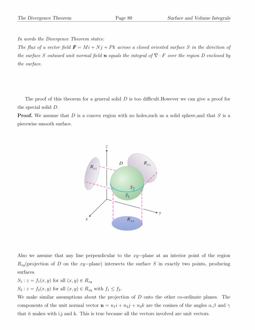
The Divergence Theorem Page 80 Surface and Volume Integrals
In words the Divergence Theorem states:
The flux of a vector field F = Mi + Nj + Pk across a closed oriented surface S in the direction of
the surface S outward unit normal field n equals the integral of ∇ · F over the region D enclosed by
the surface.
The proof of this theorem for a general solid D is too difficult.However we can give a proof for
the special solid D.
Proof. We assume that D is a convex region with no holes,such as a solid sphere,and that S is a
piecewise smooth surface.
Also we assume that any line perpendicular to the xy−plane at an interior point of the region
Rxy(projection of D on the xy−plane) intersects the surface S in exactly two points, producing
surfaces.
S1 : z = f1(x, y) for all (x, y) ∈ Rxy
S2 : z = f2(x, y) for all (x, y) ∈ Rxy with f1 ≤ f2.
We make similar assumptions about the projection of D onto the other co-ordinate planes. The
components of the unit normal vector n = n1i + n2j + n3k are the cosines of the angles α,β and γ
that n makes with i,j and k. This is true because all the vectors involved are unit vectors.
80

Surface and Volume Integrals Page 81 The Divergence Theorem
We have n1 = n · i = |n|i| cosα = cosα, n2 = n · j = cos β and n3 = n · k = cos γ. Thus
n = (cosα)i+ (cos β)j + (cos γ)k and F · n = M cosα +N cos β + P cos γ. In component from, the
Divergence theorem states that
∫∫S
(M cosα+N cos β+P cos γ)dσ =
∫∫∫D
(∂M
∂x+∂N
∂y+∂P
∂z)dxdydz
. We prove the theorem by proving the three following equalities∫∫S
M cosαdσ =
∫∫∫D
∂M
∂xdxdydz.. . . [2]∫∫
S
N cos βdσ =
∫∫∫D
∂N
∂ydxdydz.. . . [3]∫∫
S
P cos γdσ =
∫∫∫D
∂P
∂zdxdydz.. . . [4]
We prove equation[4] by converting the surface integral on the left to a double integral over the
projection Rxy of D on the xy−plane.
81

The Divergence Theorem Page 82 Surface and Volume Integrals
The surface S consists of an upper part S2 whose equation is Z = f2(x, y) and a lower part S1 whose
equation is Z = f1(x, y). On S2, the outer normal n has a positive k-component and cos γdσ = dxdy
because dσ =dA
cos γ=dxdy
cos γ.On S1, the outer normal n has a negative k-component and cos γdσ =
−dxdy
Therefore
∫∫S
P cos γdσ =
∫∫S2
P cos γdσ +
∫∫S1
P cos γdσ
=
∫∫Rxy
P (x, y, f2(x, y))dxdy −∫∫
Rxy
P (x, y, f1(x, y))dxdy
=
∫∫Rxy
[P (x, y, f2(x, y))dxdy − P (x, y, f1(x, y))]dxdy
=
∫∫Rxy
[
∫ f2(x,y)
f1(x,y)
∂p
∂zdz]dxdy =
∫∫∫D
∂p
∂zdzdxdy
This proves equation [4].
The proof for [2] and [3] follow the same pattern of just permute x, y, z;M,N,P ; α, β, γ in order,
and get those results from equation [4].
The divergence Theorem for other regions:-
The Divergence Theorem can be extended to regions that can be partitioned into a finite number
of simple regions of the type just discussed and to regions that can be defined as limits of simpler
regions in certain ways. Suppose that D is the region between two concentric spheres and that F
has continuously differentiable components throughout D and on the bounding surfaces. Split D by
an equatorial plane and apply the Divergence theorem to each half separately. The bottom half D1
is shown in figure.
82
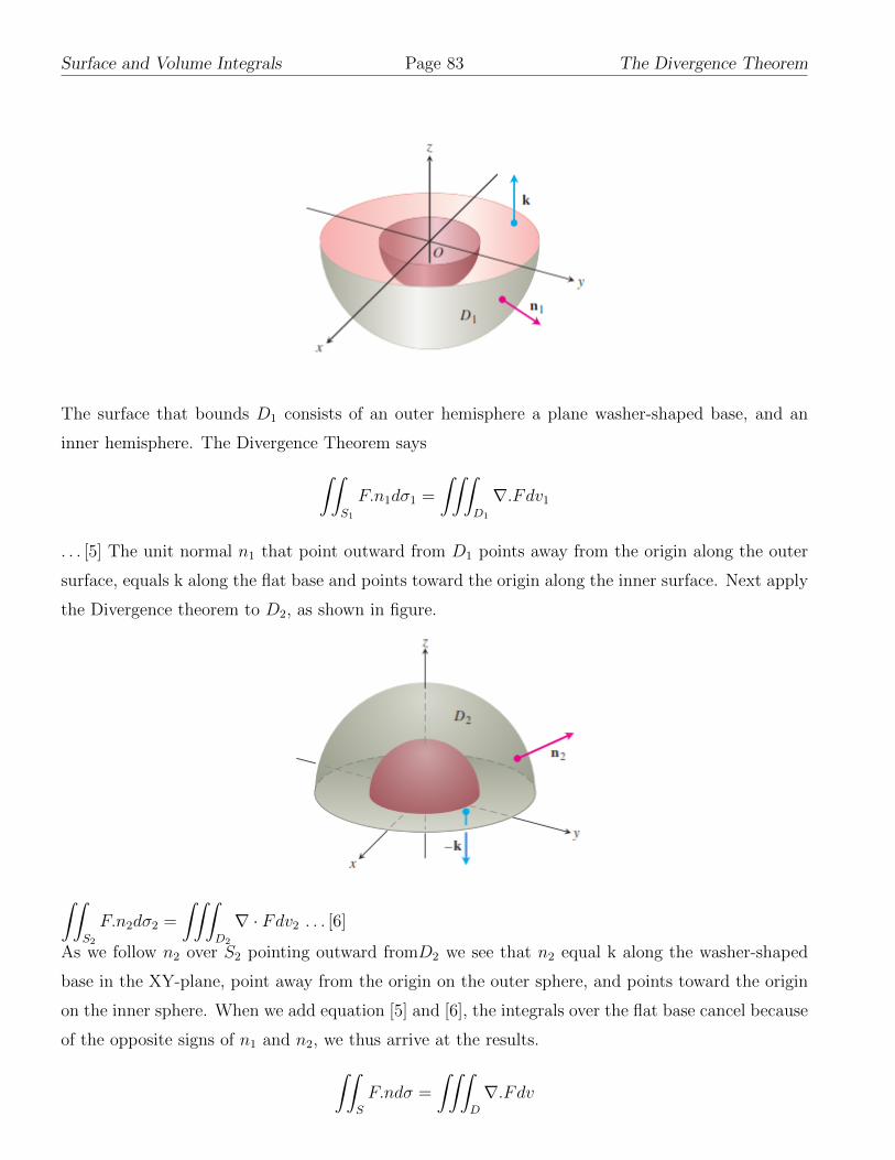
Surface and Volume Integrals Page 83 The Divergence Theorem
The surface that bounds D1 consists of an outer hemisphere a plane washer-shaped base, and an
inner hemisphere. The Divergence Theorem says∫∫S1
F.n1dσ1 =
∫∫∫D1
∇.Fdv1
. . . [5] The unit normal n1 that point outward from D1 points away from the origin along the outer
surface, equals k along the flat base and points toward the origin along the inner surface. Next apply
the Divergence theorem to D2, as shown in figure.
∫∫S2
F.n2dσ2 =
∫∫∫D2
∇ · Fdv2 . . . [6]
As we follow n2 over S2 pointing outward fromD2 we see that n2 equal k along the washer-shaped
base in the XY-plane, point away from the origin on the outer sphere, and points toward the origin
on the inner sphere. When we add equation [5] and [6], the integrals over the flat base cancel because
of the opposite signs of n1 and n2, we thus arrive at the results.∫∫S
F.ndσ =
∫∫∫D
∇.Fdv
83
The Divergence Theorem Page 84 Surface and Volume Integrals
, where D is the region between the spheres S the boundary of D consisting of two spheres, and n
the unit normal to S directed outward from D.
Example 3.22. Find
∫∫S
F.nds where F = xi− yj + (z2 − 1)k and S is the cylinder formed by
the surface z = 0, z = 1, x2 + y2 = 4
Solution. Here F = xi− yj + (z2 − 1)k ∴ DivF =∂
∂x(x) +
∂
∂y(−y) +
∂
∂z(z2 − 1)
= 1− 1 + 2z = 2z
By Gauss’s divergence theorem
∫∫S
F.nds =
∫∫∫V
divFdV
=
∫ 2
−2
∫ √4−x2
−√
4−x2
∫ z=1
z=0
dxdydz =
∫ 2
−2
∫ √4−x2
−√
4−x2
[z2]1
0dxdy
=
∫ 2
−2
∫ √4−x2
−√
4−x2dxdy
= 2
∫ 2
−2
√4− x2dx
= 4
[1
2x√
4− x2 +4
2sin−1x
2
]2
−2
= 4
[4
2.π
2
]= 4π.
Example 3.23. Show that
∫∫S
(axi+ byj + czk) · nds =4
3π (a+ b+ c) where S is the surface of
the sphere x2 + y2 + z2 = 1.
Solution. :Here F = axi+ byj + czk
∴ divF =∂
∂x(ax) +
∂
∂y(by) +
∂
∂z(cz)
= a+ b+ c.
∴ By Gauss’s Divergence Theorem∫∫S
(axi+ byj + czk) · nds
=
∫∫∫V
divFdV =
∫∫∫V
(a+ b+ c)dV
= (a+ b+ c)
∫∫∫V
dV = (a+ b+ c)V
=4
3(a+ b+ c)π as V =
4
3π, being the volume of the sphere of unit radius.
84

Surface and Volume Integrals Page 85 The Divergence Theorem
Example 3.24. Apply Gauss’s divergence theorem to evaluate
∫∫S
[(x3 − yz
)dydz − 2x2ydzdx+ zdxdy
]over the surface of a cube bounded by co-ordinate planes and the planes x = y = z = a
Solution. :Gauss’s Divergence theorem in cartesian co-ordinates states that
∫∫S
(F1dydz + F2dzdx+ F3dxdy)
=
∫∫∫V
(∂F1
∂x+∂F2
∂y+∂F3
∂z
)dxdydz
Here F1 = x3 − yz, F2 = −2x2y, F3 = z then∂F1
∂x= 3x2,
∂F2
∂y= 2x2,
∂F3
∂z= 1
Hence using the above theorem, we have
∫∫S
[(x3 − yz
)dydz − 2x2ydzdx+ zdxdy
]=
∫ a
0
∫ a
0
∫ a
0
(3x2 − 2x2 + 1)dxdydz
=
∫ a
0
∫ a
0
∫ a
0
(x2 + 1)dxdydz
=
∫ a
0
∫ a
0
[x3
3+ x
]a0
dydz
=1
3a5 + a3.
Example 3.25. Verify divergence theorem for F = (x2 − yz) i+ (y2 − zx) j + (z2 − xy) k ,taken
over the rectangular parallelopiped 0 ≤ x ≤ a,
0 ≤ y ≤ b,0 ≤ z ≤ c.
Solution. : We have divF = ∇ · F=
∂
∂x(x2 − yz) +
∂
∂y(y2 − zx) +
∂
∂z(z2 − xy)
= 2 (x+ y + z) By gauss’s Divergence theorem
∫∫S
F · nds =
∫∫∫V
∇ · FdV
=
∫ a
x=0
∫ b
y=0
∫ c
z=0
2 (x+ y + z) dxdydz
=
∫ a
x=0
∫ b
y=0
[xz + yz +
z2
2
]cz=0
dxdy
= 2
∫ a
x=0
∫ b
y=0
(xc+ yc+
c2
2
)dxdy
= 2
∫ a
x=0
[xyc+
y2
2c+
c2
2y
]by=0
dx
= 2
∫ a
x=0
(xbc+
b2
2c+
c2
2b
)dx
= 2
[x2
2bc+
b2
2cx+
c2
2bx
]a0
= a2bc+b2ca+c2ba = abc (a+ b+ c) Verification:[fig 3.4.6]To calculate directly the value of
∫∫S
F ·nds
85

The Divergence Theorem Page 86 Surface and Volume Integrals
over the six faces of the rectangular parallelopiped over the face DEFG, equation of the plane is
x = a,dx = 0 and n = i ∴ over the face DEFG =
∫∫∫DEFG
F · nds
=
∫ c
z=0
∫ b
y=0
[(a2 − yz
)i+(y2 − za
)j +
(z2 − ay
)k]idydz
=
∫ c
z=0
∫ b
y=0
(a2 − z
)dydz (since j · i = 0 = k · j)∫ c
z=0
[a2y − zy2
2
]b0
dz∫ c
z=0
[a2b− zb2
2
]dz
=
[a2bz − z2b2
4
]c0
= a2bc− c2b2
4Similarly over the face ABCO,n = −i, x = 0 =
∫∫∫ABCO
F · nds
=
∫ c
z=0
∫ b
y=0
[(0− yz) i+ (· · · ) j + (· · · ) k] (−i) dydz
=
∫ c
z=0
∫ b
y=0
yzdydz =
∫ c
0
y2
2zdz
=
∫ c
0
b2
2zdz =
b2c2
4Over the face ABEF,n = j, y = b
∴ =
∫∫∫ABEF
F · nds
=
∫ c
z=0
∫ a
x=0
[(x2 − bz
)i+(b2 − xz
)j +
(z2 − xb
)k]
(j) dxdz
=
∫ c
z=0
∫ a
x=0
(b2 − xz
)dxdz =
∫ c
0
[b2x− x2
2z
]a0
dz
=
∫ c
0
(b2a− a2z
2
)dz
= b2ac− a2c2
4Over the face OGDC,n = −j, y = 0
∴ =
∫∫∫OGDC
F · nds
=
∫ c
z=0
∫ a
x=0
xzdxdz
=c2a2
4Over the face BCDE,n = k, Z = C
∴ =
∫∫∫BCDE
F · nds
=
∫ b
y=0
∫ a
x=0
(c2 − xy
)dxdy
= c2ab− a2b2
4Over the face AFGO,n = −k, Z = 0
86

Surface and Volume Integrals Page 87 The Divergence Theorem
∴ =
∫∫∫ARGO
F · nds
=
∫ b
y=0
∫ a
x=0
(−xy) dxdy
=a2b2
4
Hence over all the six faces of the cube.
∫∫S
F ·nds =
(a2bc− c2b2
4
)+b2c2
4+
(b2ac− a2c2
4
)+c2a2
4
+
(c2ab− a2b2
4
)+a2b2
4= abc (a+ b+ c)
Hence the theorem is verfied.
Example 3.26. Apply Gauss’s divergence theorem to show that
∫∫S
r ·nds = 3V , where V is the
volume of the space enclosed by the surface S.
Solution.
∫∫S
r · nds =
∫∫S
(xi+ yj + zk) · nds
=
∫∫∫V
div (xi+ yj + zk) dV (since Gauss divergence theorem)
=
∫∫∫V
divrdV =
∫∫∫V
3dV = 3V
Example 3.27. Evaluate
∫∫S
(xi+ yj + z2k
)· nds where S is the closed surface bounded by the
cone x2 + y2 = z2 and the plane z = 1.
Solution. divF =∂
∂x(x) +
∂
∂y(y) +
∂
∂z(z2)
= 1 + 1 + 2z = 2 (1 + z)
∴ By Gauss’s divergence theorem∫∫S
(xi+ yj + z2k
)· nds =
∫∫∫V
div(xi+ yj + z2k
)dV
=
∫ 1
x=−1
∫ √1−x2
y=−√
1−x2
∫ 1
z=0
2 (1 + z) dxdydz
=
∫ 1
x=−1
∫ √1−x2
y=−√
1−x23dxdy
= 6
∫ 1
x=−1
√1− x2dx
= 12[1
2x√
1− x2 +1
2sin−1 1]10
87

Exercise Page 88 Surface and Volume Integrals
= 12.1
2· π
2= 3π.
Problem Set IV
(1) If S is any closed surface enclosing a volume V and F = xi+ 2yj + 3zk, prove that
∫∫S
F ·nds = 6V
(2) Evaluate
∫∫S
(x3dydz + x2ydzdx+ x2z
)dxdy, where S is the closed surface consisting of
the cylinder, x2 + y2 = a2 and the circular discs z = 0and z = b
(3) Verify the divergence theorem for F = 4xi− 2y2i + z2k, taken over the region bounded by
the surface x2 + y2 = 4,z = 0, z = 3.
(4) Verify the Guauss’s divergence theorem for the field F = xi + yj + zk over the sphere
x2 + y2 + z2 = a2.
(5) Evaluate
∫∫S
F · nds, where F = 4xzi − y2j + 4zk and S is the surface bounded by 2x +
2y + z, x = 0, y = 0, z = 0.
(6) Verify the divergence theorem for the function F = 4xz−y2j+yzk voer a unit cube bounded
by x = 0, x = 1, y = 0, y = 1, z = 0, z = 1.
(7) Prove that
∫∫∫V
dV
r2=
∫∫S
V · nr2
dS.
5. Exercise
(1) Find the centroid of the portion of the sphere x2 + y2 + z2 = a2 that lies in the first octant.
(2) Find the center of mass and moment of inertia and radius of gyaration about the Z-axis of
a thin shell of constant density δ cut from the cone x2 + y2 − z2 = 0 by the planes z = 1
and z = 2.
(3) Use a parametrizatin to find the flux
∫∫bfS
F.ndσ if F = z2i + xj − 3zk outward through
the surface cut from the parabolic cylinder z = 4− y2 by the planes x = 0, x = 1 and z = 0.
(4) Use a parametrization to find the flux
∫∫S
F.ndσ if F = zk across the portion of the sphere
x+2 +y2 + z2 = a2 in the first octant in the direction away from the origin.
(5) Evaluate
∫∫S
(∇× F ).ndσ for F = (2x− y + z)i+ (x+ y − z2)j + (3x− 2y + 4z)k over the
surface of the cylinder x2 + y2 = 4 bounded by the plane z = 9 and open end z = 0.
(6) Use a parametrization to find the flux of F = yzi+ xj− z2k outward through the parabolic
cylinder y = x2, 0 ≤ x ≤ 1, 0 ≤ z ≤ 4
(7) Calculate Flux ofF where F = xi+ yj + 2zk over the surface x2 + y2 + z2 = a2.
(8) Evaluate
∫∫S
√(a2x2 + b2y2 + c2z2)dS over the ellipsoid ax2 + by2 + cz2 = 1.
88

Surface and Volume Integrals Page 89 Exercise
(9) Evaluate
∫∫S
F ·ndS where F = (y − x) i+ (z − y) j + (y − x) k, over the cube bounded by
the plane x± 1, y ± 1, z ± 1
(10) using the divergence theorem to calculate outward flux of F across the boundary of the
region D
(a) F = yi + xyj − zk, D: The region inside the solid cylinder x2 + y2 ≤ 4 between the
plane z = 0 and the paraboloid z = x2 + y2
(b) F = x2i− 2xyj + 3zk, D: The region cut from the first octant by the sphere
x2 + y2 + z2 = 4.
89

Answers Page 90 Surface and Volume Integrals
6. Answers
6.1. Problem Set I. (1)62π
3(2) 4 (3)
abc
4(ab+ ac+ bc) (4) 9a3 (5) 81 (6)
3
2(7) 18 (8)
πa3
2.
6.2. Problem Set II.
(1) r(r, θ) = (r cos θ)i + (r sin θ)j +√
9− r2k, 0 ≤ r ≤ 3√
2
2, 0 ≤ θ ≤ 2π. Also r(φ, θ) =
(3 sinφ cos θ)i+ (3 sinφ sin θ)j + (3 cosφ)k, 0 ≤ φ ≤ π
4, 0 ≤ θ ≤ 2π.
(2) r(r, v) = ui+ (3cosv)j + (3sinv)k, 0 ≤ u ≤ 3, 0 ≤ v ≤ 2π.
(3) r(r, v) = 4cos2vi + (u)j + (4cosvsinv)k, 0 ≤ u ≤ 3, −π2≤ v
π
2. or r(u, v) = (2 + 2cosu)i +
uj + (2sinv)K, 0 ≤ u ≤ 3, 0 ≤ v ≤ 2π.
(4)
∫ 2π
0
∫ 1
0
√5
2drdθ =
π√
5
2
(5)
∫ 2π
0
∫ 3
1
r√
5drdθ = 8π√
5.
(6)
∫ 2π
0
∫ π
π/4
2 sinφdφdθ = (4 + 2√
2)π.
(7)
∫∫S
xdσ =
∫ 3
0
∫ 2
0
u√
4u2 + 1dudv =17√
17− 1
4.
(8)
∫∫S
x2dσ =
∫ 2π
0
∫ π
0
sin3 φ cos2 θdφdθ =4π
3.
6.3. Problem Set III. 1. a. 4π ,b. −5/6 ,c. 0
2. a. 12π, b. −π/4
6.4. Problem Set IV. (1) 6V (2)5
4πa4b (3) common value= 84π (4) 4πa3 (5)
−81
4(6) Common
value =3
2
6.5. Exercise. (1) (a
2,a
2,a
2) (2) (x, y, z) = (0, 0,
14
9), Iz =
15π√
2
2δ, Rz =
√10
2(3) −32 (4)
πa3
6
(5) 8π (6) 2 (7)16πa3
3(8)
4π√abc
(9) −16 (10) (a) −8π (b) 3π
90