Scalable Traffic Quality and System EfficiencyIndicators Towards Overall Telecommunication

System’s QoE Management

Stoyan Poryazov1(✉) , Emiliya Saranova1,2 , and Ivan Ganchev1,3,4

1 Institute of Mathematics and Informatics, Bulgarian Academy of Sciences,Sofia, Bulgaria

stoyan@math.bas.bg, emiliya@cc.bas.bg2 University of Telecommunications and Post, Sofia, Bulgaria

3 University of Limerick, Limerick, Irelandivan.ganchev@ul.ie

4 University of Plovdiv “Paisii Hilendarski”, Plovdiv, Bulgaria

Abstract. Conceptual and analytical models of an overall telecommunicationsystem are utilized in this chapter for the definition of scalable indicators towardsQuality of Service (QoS) monitoring, prediction, and management. The telecom‐munication system is considered on different levels – service phase, service stage,network, and overall system. The network itself is presented in seven service stages– A-user, A-terminal, Dialing, Switching, B-terminal Seizure, B-terminal, and B-user, each having its own characteristics and specifics. Traffic quality indicators areproposed on each level. Two network cost/quality ratios are proposed – mean andinstantaneous – along with illustrative numerical predictions of the latter, whichcould be useful for dynamic pricing policy execution, depending on the networkload. All defined indicators could be considered as sources for Quality of Experi‐ence (QoE) prediction.

Keywords: Overall telecommunication system · Performance modelDynamic quality of service (QoS) · Telecommunication subservicesDifferentiated QoS subservice indicator · QoS prediction · Human factors of QoSInstantaneous Cost/Quality Ratio · Quality of Experience (QoE)

1 Introduction

Starting from 2010, e.g. [1], a new attitude towards the Quality of Service (QoS) hasbecome dominant, namely to consider QoS and Quality of Experience (QoE) as goods,and the usage of Experience Level Agreement (ELA) [2] has started to be discussed.The importance of the teletraffic models, particularly of the overall QoS indicators, forQoE assessment is emphasized by Fiedler [3]. Until now, however, the usage ofperformance models of overall telecommunication systems was not very popular. Thischapter utilizes the models, elaborated in the Chapter “Conceptual and AnalyticalModels for Predicting the Quality of Service of Overall Telecommunication Systems”of this book, for the definition of scalable QoS indicators towards overall

© The Author(s) 2018I. Ganchev et al. (Eds.): Autonomous Control for a Reliable Internet of Services, LNCS 10768, pp. 81–103, 2018.https://doi.org/10.1007/978-3-319-90415-3_4

telecommunication system’s QoS monitoring, prediction, and management. Some indi‐cators reflect predominantly the users’ experience. All defined indicators depend onhuman (users’) characteristics and technical characteristics, and may be considered assources for QoE prediction.

For this, in Sect. 2, traffic characterization of a service in a real device (service phase)is first elaborated. Definitions of served-, carried-, parasitic-, ousted-, and offered carriedtraffic are proposed, based on the ITU-T definitions, and eight service phase trafficquality indicators are proposed.

In Sect. 3, the service stage concept is developed and corresponding traffic qualityindicators are defined.

In Sect. 4, telecommunication system and network efficiency indicators are proposedas follows: eight indicators – on the service stage level, five indicators – on the networklevel, and three indicators – on the overall system level. The relationship between indi‐cators on the service stage-, network-, and system level are described. A comparisonwith classical network efficiency indicators is made. The applicability of the approachand results obtained for defining other indicators, as well as for numerical prediction ofindicators’ values, is shown.

In Sect. 5, two network cost/quality ratios are proposed – mean and instantaneous –and illustrative numerical predictions of the latter are presented, which may be usefulfor dynamic pricing policy execution, depending on the network load.

In the Conclusion, possible directions for future research are briefly discussed.

2 Service Phase Concept and Traffic Quality Indicators

The conceptual model utilized in this chapter is described in detail in the Chapter“Conceptual and Analytical Models for Predicting the Quality of Service of OverallTelecommunication Systems” of this book. It consists of five levels: (1) overall tele‐communication system and its environment; (2) overall telecommunication network;(3) service stages; (4) service phases; and (5) basic virtual devices. In the followingsubsections, the concepts of ‘service phase’ and ‘service stage’ are elaborated.

2.1 Service Phase

Based on the ITU-T definition of a service, provided in [4] (Term 2.14), i.e. “A set offunctions offered to a user by an organization constitutes a service”, we propose thefollowing definition of a service phase.

Definition 1: The Service Phase is a service presentation containing:

• One of the functions, realizing the service, which is considered indivisible;• All modeled reasons for ending/finishing this function, i.e. the causal structure of the

function;• Hypothetic characteristics, related to the causal structure of the function (a well-

known example of a hypothetic characteristic is the offered traffic concept).

82 S. Poryazov et al.

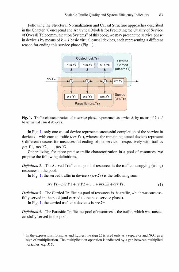
Following the Structural Normalization and Causal Structure approaches describedin the Chapter “Conceptual and Analytical Models for Predicting the Quality of Serviceof Overall Telecommunication Systems” of this book, we may present the service phasein device s by means of k + 1 basic virtual causal devices, each representing a differentreason for ending this service phase (Fig. 1).

OfferedCarried

(ofr.crr.Ys)

srv.Fs

ous.Yk

Served(srv.Ys)

2

ous.Y2ous.Y1

crr.Ys1 k

prs.Yk

Parasitic (prs.Ys)

Ousted (ost.Ys)

prs.Y2prs.Y1

Fig. 1. Traffic characterization of a service phase, represented as device S, by means of k + 1basic virtual causal devices.

In Fig. 1, only one causal device represents successful completion of the service indevice s – with carried traffic (crr.Ys1), whereas the remaining causal devices representk different reasons for unsuccessful ending of the service – respectively with trafficsprs.Y1, prs.Y2, … , prs.Yk.

Generalizing, for more precise traffic characterization in a pool of resources, wepropose the following definitions.

Definition 2: The Served Traffic in a pool of resources is the traffic, occupying (using)resources in the pool.

In Fig. 1, the served traffic in device s (srv.Ys) is the following sum:

srv.Ys= prs.Y1+ rs.Y2+ … + prs.Yk+ crr.Ys . (1)

Definition 3: The Carried Traffic in a pool of resources is the traffic, which was success‐fully served in the pool (and carried to the next service phase).

In Fig. 1, the carried traffic in device s is crr.Ys.

Definition 4: The Parasitic Traffic in a pool of resources is the traffic, which was unsuc‐cessfully served in the pool.

1 In the expressions, formulas and figures, the sign (.) is used only as a separator and NOT as asign of multiplication. The multiplication operation is indicated by a gap between multipliedvariables, e.g. X Y.

Scalable Traffic Quality and System Efficiency Indicators 83

In Fig. 1, each of traffics prs.Y1, prs.Y2, … , prs.Yk is a parasitic one. Parasitictraffic occupies real resources but not for an effective service execution.

In Definitions 2 and 3, the served- and carried traffic are different terms, despite theITU-T definition of the carried traffic as “The traffic served by a pool of resources” ([5],Term 5.5). We believe that this distinction leads to a better and more detailed traffic-and QoS characterization.

Definition 5: The Ousted Traffic is the traffic that would be carried, if there is no unsuc‐cessful service ending in the pool of resources.

In Fig. 1, each parasitic traffic prs.Y1, prs.Y2, … , prs.Yk ousts a correspondingtraffic that would be carried, if there is no unsuccessful service ending of the corre‐sponding type: ous.Y1, ous.Y2, … , ous.Yk. The flow intensity to a parasitic device andthe corresponding ousted device is the same by definition, i.e.:

ous.Fi = prs.Fi, for i= [1, k], (2)

but the service times are different.The hypothetic service time for every ousted device (ous.Ti) equals the carried

service time (crr.Ts):

ous.Ti = crr.Ts, for i= [1, k] . (3)

The ousted traffic is a hypothetic one with the following intensity:

ous.Yi = prs.Fi crr.Ts, for i= [1, k] . (4)

2.2 Causal Generalization

In the Chapter “Conceptual and Analytical Models for Predicting the Quality of Serviceof Overall Telecommunication Systems” of this book, the causal presentation and causalaggregation are discussed. The causal aggregation is understood as an aggregation ofall cases in the model, corresponding to different reasons for service ending (referred toas unsuccessful cases further in this chapter).

Here a causal generalization is proposed, as an aggregation of all unsuccessful cases(prs.Ys). Besides this, an aggregation of all cases of ousted traffic (ous.Ys) could be used:

prs.Ys=

k∑

i=1

prs.Yi; (5)

ous.Ys=

k∑

i=1

ous.Yi. (6)

By Definition 2, the served traffic is a sum of the parasitic and carried traffic (c.f.Fig. 1):

84 S. Poryazov et al.

srv.Ys= prs.Ys+ crr.Ys; (7)

srv.Fs= prs.Fs+ crr.Fs . (8)

If the system is considered as being in a stationary state, by using the Little’s formula[6] we have: prs.Ys = prs.Fs prs.Ts and crr.Ys= crr.Fs crr.Ts . Hence:

srv.Ys= srv.Fs srv.Ts = prs.Fs prs.Ts + crr.Fs crr.Ts . (9)

Formulas (7), (8), and (9) illustrate the advantage of the traffic qualifiers – the nota‐tion is invariant to the number of cases considered in a service phase.

2.3 Offered Carried Traffic

Definition 6: The Offered Carried Traffic (ofr.crr.Ys) in a pool s of resources is the sumof the carried traffic (crr.Ys) and ousted traffic (ous.Ys) in the pool:

ofr.crr.Ys = ous.Ys + crr.Ys. (10)

From (10), (6), (4), (8), prs.Fs =k∑

i=1prs.Fi and crr.Ys = crr.Fs crr.Ts, the following

formula could be obtained:

ofr.crr.Ys = srv.Fs crr.Ts.

Definition 6 is analogous to the ITU-T definition of an Equivalent Offered Traffic [7]but considers the traffic related to the carried call attempts, whereas the ITU-T definitionconsiders the traffic that would be served.

2.4 Traffic Quality Indicators

Indicator 1: Offered Carried Traffic Efficiency – the ratio of the carried traffic, in aservice phase, to the offered carried traffic:

I1 =crr.Ys

ofr.crr.Ys= 1 −

ous.Ys

ofr.crr.Ys. (11)

Indicator 2: Causal Ousted Importance – the ratio of the ousted traffic due toreason i (ous.Yi) to the offered carried traffic of a service phase (ofr.crr.Ys):

I2(i) =ous.Yi

ofr.crr.Ys. (12)

This indicator allows the estimation of missed benefits due to reason i and thereforethe necessity of countermeasures against this reason.

Indicator 3: Ousted Traffic Importance – the sum of all causal ousted importanceindicators of a service phase. From Fig. 1, and Formulas (6) and (11), it is:

Scalable Traffic Quality and System Efficiency Indicators 85

I3 =

k∑

i=1

I2(i) =

k∑

i=1

ous.Yi

ofr.crr.Ys=

ous.Ys

ofr.crr.Ys= 1 −

crr.Ys

ofr.crr.Ys. (13)

Indicator 4: Service Efficiency – the ratio of the carried traffic to the served traffic:

I4 =crr.Ys

srv.Ys= 1 −

prs.Ys

srv.Ys. (14)

Indicator 5: Causal Parasitic Importance – the ratio of the parasitic traffic due toreason i (prs.Yi) to the served traffic of a service phase (srv.Ys):

I5(i) =prs.Yi

srv.Ys. (15)

This indicator allows the estimation of an ineffective service due to a reason andtherefore the necessity of countermeasures against this reason.

Indicator 6: Parasitic Traffic Importance – the sum of all causal parasitic impor‐tance indicators of a service phase. From Fig. 1, and Formulas (5) and (14), it is:

I6 =

k∑

i=1

I5(i) =

k∑

i=1

prs.Yi

srv.Ys=

prs.Ys

srv.Ys= 1 −

crr.Ys

srv.Ys. (16)

Indicator 7: Ousted/Parasitic Traffic Ratio – this is the ratio of the ousted trafficto the parasitic traffic:

I7 =ous.Ys

prs.Ys. (17)

This indicator estimates the aggregated, by all reasons, ratio of missed benefits tothe ineffective service in a service phase.

Indicator 8: Causal Ousted/Parasitic Traffic Ratio – this is the ratio of the oustedtraffic, due to reason i, to the parasitic traffic due to the same reason. From Definition 5and Formula (2):

I8(i) =ous.Yi

prs.Yi=

ous.Ti

prs.Ti. (18)

This indicator gives another important estimation of a reason for ineffective servicein a service phase.

3 Service Stage Concept and Traffic Quality Indicators

Definition 7: The Service Stage is a service presentation containing:

• One service phase, realizing one function of the service;

86 S. Poryazov et al.

• All auxiliary service phases that directly support this function realization but are notpart of the realized function itself.

Examples of auxiliary service phases are the entry, exit, buffer, and queue virtualdevices. The performance of the auxiliary devices depends directly on the service phase,realizing a function of the service.

The service stage concept allows the division of the overall telecommunicationservice into subservices and therefore makes easier the system modeling process.

3.1 Service Stage

For simplicity in this subsection, the simplest possible service stage, consisting of onlytwo service phases, is considered (Fig. 2). For more complex service stages with morephases, please refer to the Chapter “Conceptual and Analytical Models for Predictingthe Quality of Service of Overall Telecommunication Systems” of this book.

srv.Fs

blc.Ys

ofr.Fg

Blocked(blc.Ys)

Served(srv.Ye)

ous.Ys

Served(srv.Ys)prs.Ys

crr.Ys

ofr.crr.Ys

ous.Ye

crr.Ye

prs.Ye

ofr.crr.Ye

EntranceDevice

ServiceDevice

crr.Fg

prs.Fg

Stage g

Fig. 2. A service stage g, consisting of Entrance and Service phases.

The service stage g, in Fig. 2. consists of Entrance and Service phases (representedby corresponding virtual devices). The Entrance device (e) may check the service request(call) attempt for having the relevant admission rights, whereas the Service device (s)checks for service availability or existence of free service resources, etc. Let ofr.Fg isthe flow intensity of the service request attempts offered to this stage, crr.Fg – the inten‐sity of the outgoing carried flow, prs.Fg – the flow intensity of the parasitic servedrequests, and prs.Fe – the intensity of the parasitic call attempts flow. Then from Fig. 2we have:

Scalable Traffic Quality and System Efficiency Indicators 87

prs.Fe = ofr.Fg prs.Pe, (19)

where prs.Pe is the probability of directing the service request attempts to the general‐ized parasitic service in device e. By analogy:

prs.Fs = ofr.Fg (1 − prs.Pe) prs.Ps. (20)

The total parasitic flow in service stage g is:

prs.Fg = prs.Fe + prs.Fs. (21)

The carried traffic (crr.Yg) in service stage g is a sum of the carried traffic in devicese and s:

crr.Yg = crr.Ye + crr.Ys = crr.Fe crr.Te + crr.Fs crr.Ts, (22)

where:

crr.Fe = ofr.Fg (1 − prs.Pe); (23)

crr.Fs = ofr.Fg (1 − prs.Pe) (1 − prs.Ps). (24)

The total carried traffic in service stage g is:

crr.Yg = ofr.Fg (1 − prs.Pe) ( crr.Te + (1 − prs.Ps) crrTs). (25)

The estimation of the carried traffic in a service stage could be problematic due tothe fact that some of the carried service requests attempts in the first device (e) are notcarried to the next device (s), i.e. they become parasitic service requests with probabilityprs.Ps (c.f. Fig. 2).

Based on the ITU-T definition of ‘effective traffic’ [5], i.e. as “The traffic corre‐sponding only to the conversational portion of effective call attempts”, we propose herethe Effective Carried Traffic concept.

Definition 8: The Effective Carried Traffic in a service stage is the traffic correspondingto the service request attempts leaving the stage with a fully successful (carried) service.

In Fig. 2, the effective carried traffic (eff.crr.Yg) of service stage g is:

eff .crr.Yg = eff .crr.Fg eff .crr.Tg, (26)

where:

eff .crr.Fg = crr.Fs = ofr.Fg (1 − prs.Pe)(1 − prs.Ps); (27)

eff .crr.Tg = crr.Te + crr.Ts. (28)

From (26), (27), and (28), we obtain:

eff .crr.Yg = ofr.Fg (1 − prs.Pe)(1 − prs.Ps)(crr.Te + crr.Ts). (29)

88 S. Poryazov et al.

Note the difference between (25) and (29), i.e. in general, in a service stage, theeffective carried traffic is less than the carried traffic.

The Offered Traffic is a fundamental teletraffic engineering concept. We use theITU-T definition of the Equivalent Offered Traffic [7], i.e. “Offered traffic, to a pool ofresources, is the sum of carried and blocked traffic of this pool”.

The blocked traffic corresponds to the blocked attempts, as per Definition 2.8 in [5]:“Blocked call attempt: A call attempt that is rejected owing to a lack of resources in thenetwork”. This definition, however, is too narrow to be applied directly to blockedservice request attempts as it does not include most of the reasons for rejection, includingaccess control, service unavailability, called terminal unavailability or busyness, andmany others. Thus we propose the following extension of it.

Definition 9: The Blocked Service Request Attempt is a service request attempt withrejected service, in the intended pool of resources, due to any reason.

Blocked traffic is a service stage concept because it considers blocking of servicerequests before entering the service phase, or in other words, blocking that occurs inanother virtual device before the corresponding service device.

In Fig. 2, blocking occurs in the Entrance device. The blocked traffic (blc.Ys) corre‐sponds to the service request attempts offered to service stage g (ofr.Fg), but notbelonging to the served attempts (srv.Fs). From Fig. 2 and the Little’s theorem, weobtain:

blc.Ys = blc.Fs blc.Ts. (30)

The service request attempts that are not carried in phase e, and hence are rejectedto the next service phase, are considered parasitic in phase e. For the intensity of theblocked attempts, the following equality holds:

blc.Fs = prs.Fe = ous.Fe = ofr.Fg prs.Pe. (31)

The offered traffic is a hypothetic one “that would be served” if it is not blocked, andtherefore:

blc.Ts = srv.Ts (32)

From (30), (31), and (32), we obtain the following formula:

blc.Ys = ofr.Fg prs.Pe srv.Ts, (33)

which is valid for the generalized reason for service request attempts rejection in servicephase e (i.e. in the Entrance device).

From the definition of the equivalent offered traffic, Fig. 2, and Formulas (23), (33),and srv.Fs = crr.Fe, the traffic offered to the service device s is:

ofr.Ys = blc.Ys + srv.Ys = ofr.Fg srv.Ts. (34)

Scalable Traffic Quality and System Efficiency Indicators 89

3.2 Traffic Quality Indicators

Many of the service-stage traffic quality indicators may be reformulated as service-stageperformance indicators as done below.

Indicator 9: Carried Effectiveness of a Service Stage – the ratio of the effectivecarried traffic to the carried traffic:

I9 =eff .crr.Y

crr.Y. (35)

For instance, from (25) and (29), the Carried Effectiveness of service stage g inFig. 2 is:

eff .crr.Yg

crr.Yg=

(1 − prs.Ps)(crr.Te + crr.Ts)

crr.Te + (1 − prs.Ps) crr.Ts. (36)

4 Telecommunication System and Network Efficiency Indicators

4.1 Telecommunication System QoS Concept

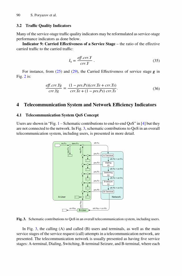
Users are shown in “Fig. 1 – Schematic contributions to end-to-end QoS” in [4] but theyare not connected to the network. In Fig. 3, schematic contributions to QoS in an overalltelecommunication system, including users, is presented in more detail.

Fig. 3. Schematic contributions to QoS in an overall telecommunication system, including users.

In Fig. 3, the calling (A) and called (B) users and terminals, as well as the mainservice stages of the service request (call) attempts in a telecommunication network, arepresented. The telecommunication network is usually presented as having five servicestages: A-terminal, Dialing, Switching, B-terminal Seizure, and B-terminal, where each

90 S. Poryazov et al.

service stage has its own characteristics. However, there are two other stages – A-userand B-user –, with their own specifics.

In Fig. 3, the possible paths of service request (call2) attempts are the following:

1. int.Fa: The calling users (A-users) generate intent call attempts, with intensityint.Fa, represented as a Generate device in the A-User block. Call intent is “Thedesire to establish a connection to a user”. “This would normally be manifested bya call demand. However, demands may be suppressed or delayed by the callinguser’s expectation of poor Quality of Service performance at a particulartime” [5].

2. sup.Fa: The intensity of suppressed intent call attempts. Suppressed traffic is “Thetraffic that is withheld by users who anticipate a poor quality of service (QoS)performance” [5]. “At present, suitable algorithms for estimating suppressed traffichave not been defined” [7].

3. dem.Fa: The intensity of demand call attempts. Call demand is: “A call intent thatresults in a first call attempt” [5].

4. rep.Fa: The intensity of repeated call attempts. Repeated call attempt is: “Any ofthe call attempts subsequent to a first call attempt related to a given call demand.NOTE – Repeated call attempts may be manual, i.e. generated by humans, or auto‐matic, i.e. generated by machines” [7].

5. ofr.Fa: The intensity of all call attempts (demand and repeated) trying to occupyA-terminals. A-terminals are considered as the first service stage (c.f. Sect. 3) inthe telecommunication network. From Fig. 3:

ofr.Fa = dem.Fa + rep.Fa. (37)

6. prs.Fa: The intensity of all parasitic (unsuccessfully served, c.f. Sect. 2) callattempts in A-terminals.We are modeling the system in a stationary state and for each considered servicestage the intensity of the offered call attempts equals the sum of the outgoing para‐sitic and carried flows, e.g. ofr.Fa = prs.Fa + crr.Fa.For each service stage, part of the parasitic attempts are terminated by the A-user(c.f. devices of type ‘terminator’ in Fig. 3) and the rest join the repeated attempt’sflow (rep.Fa).

7. ofr.Fd = crr.Fa: The intensity of carried (in A-terminals) call attempts (crr.Fa) isequal to the intensity of the offered call attempts (ofr.Fd) to the Dialing stage in thenetwork.

8. prs.Fd: The intensity of all parasitic (unsuccessfully served, c.f. Sect. 2) callattempts in the Dialing stage.

9. ofr.Fs = prs.Fs + crr.Fs: The intensity of the offered-, parasitic-, and carriedflows of call attempts of the Switching stage.

2 Throughout the rest of this chapter, the term ‘call’ should be interpreted in a broader meaningof a ‘service request’.

Scalable Traffic Quality and System Efficiency Indicators 91

10. ofr.Fz = prs.Fz + crr.Fz: The intensity of the offered-, parasitic-, and carriedflows of call attempts of the ‘B-terminal seizure’ stage. The intended B-terminalmay be busy or unavailable and this will cause blocking of call attempts.

11. ofr.Fb = prs.Fb + crr.Fb: The intensity of the offered-, parasitic-, and carriedflows of call attempts of the B-terminal stage.

12. ofr.Fbu = prs.Fbu + crr.Fbu: The intensity of the offered-, parasitic-, andcarried flows of call attempts of the B-user stage. The B-user may be absent, busy,tired, etc.

4.2 Efficiency Indicators

The efficiency indicators, proposed in this chapter, are considered on five levels: (1)service phase; (2) service stage; (3) part of network; (4) overall network; and (5) overalltelecommunication system.

4.2.1 Proposed Efficiency Indicators on Service Stage LevelIn each service stage, a basic performance indicator is the ratio between intensities ofthe carried flow and offered flow of call attempts. An exception is the A-User stagebecause there are two sub-stages in it – Ai (considering the intent call attempts) and Ad(considering the demand call attempts).

Indicator 10: Efficiency indicator Qai on the Ai sub-stage:

I10 = Qai =dem.Fa

int.Fa(38)

Indicator 11: Efficiency indicator Qad on the Ad sub-stage.Let Pr is the aggregated probability of repetition of the offered (to the A-terminals)

call attempts:

Pr =rep.Fa

ofr.Fa. (39)

From (37) and (39), the following formula could be obtained for the efficiency indi‐cator Qad:

I11 = (1 − Pr) =dem.Fa

ofr.Fa=

dem.Fa

dem.Fa + rep.Fa=

1𝛽= Qad, (40)

where β is defined in [7] as:

𝛽 =All call attempts

First call attempts. (41)

In (40), Qad is de-facto the probability corresponding to the ratio of the primary(demand) call attempts’ intensity to the offered attempts’ intensity. It may be consideredas an aggregated overall network performance indicator (as per the initial attempt in [8]).

92 S. Poryazov et al.

Indicator 12: Efficiency indicator Qa on the A-terminal stage:

I12 = Qa =crr.Fa

ofr.Fa. (42)

Indicator 13: Efficiency indicator Qd on the Dialing stage:

I13 = Qd =crr.Fd

ofr.Fd. (43)

Indicator 14: Efficiency indicator Qs on the Switching stage:

I14 = Qs =crr.Fs

ofr.Fs. (44)

Indicator 15: Efficiency indicator Qz on the ‘B-terminal Seizure’ stage:

I15 = Qz =crr.Fz

ofr.Fz. (45)

Indicator 16: Efficiency indicator Qb on the B-terminal stage:

I16 =Qb=crr.Fb

ofr.Fb. (46)

Indicator 17: Efficiency indicator Qbu on the B-user stage:

I17 =Qbu=crr.Fbu

ofr.Fbu. (47)

4.2.2 Proposed Efficiency Indicators on Network LevelNetwork efficiency indicators estimate QoS characteristics of portions of the networkcomprising more than one service stages, or the overall network. In this subsection, asusually, the indicated network portion begins with the starting points of the network andends in another network point of interest. All network efficiency indicators are fractionswith denominators offered to the A-terminals’ flow intensity ofr.Fa.

The classic network efficiency indicators are the following three, e.g. as defined in[9]:

1. “Answer Seizure Ratio (ASR) = (number of seizures that result in an answersignal)/(the total number of seizures)” … “Measurement of ASR may be made on aroute or on a destination code basis” … “A destination can be a mobile network, acountry, a city, a service, etc.” [9].

2. “Answer Bid Ratio (ABR) = (number of bids that result in an answer signal)/(totalnumber of bids); ABR is similar to ASR except that it includes bids that do not resultin a seizure” [9].

Scalable Traffic Quality and System Efficiency Indicators 93

3. “Network Effectiveness Ratio (NER): NER is designed to express the ability ofnetworks to deliver calls to the far-end terminal. NER expresses the relationshipbetween the number of seizures and the sum of the number of seizures resulting ineither an answer message, or a user busy, or a ring no answer, or in the case of ISDNa terminal rejection/unavailability. Unlike ASR, NER excludes the effects ofcustomer behavior and terminal behavior” [9].

These classic efficiency indicators reflect network providers’ attitude but don’tconsider the possibilities for initiated but unsuccessful communication as well as theinfluence of repeated attempts.

Below we propose new network efficiency indicators, all having as an index the firstletter of the last service stage considered.

Indicator 18: Network efficiency indicator Ea on the A-terminal stage, c.f. also(42):

I18 = Ea =crr.Fa

ofr.Fa= Qa = I12. (48)

Indicator 19: Network efficiency indicator Ed on the Dialing stage, c.f. also (43):

I19 = Ed =crr.Fd

ofr.Fa= Qa Qd = I12 I13. (49)

Indicator 20: By taking into account that crr.Fd = ofr.Fs, c.f. Fig. 3 and (44), thenetwork efficiency indicator Es on the Switching stage is:

I20 = Es =crr.Fs

ofr.Fa= Qa Qd Qs = I14 I19 . (50)

Indicator 21: By taking into account that crr.Fs = ofr.Fz, c.f. Fig. 3 and (45), thenetwork efficiency indicator Ez on the ‘B-terminal seizure’ stage is:

I21 = Ez =crr.Fz

ofr.Fa= Qa Qd Qs Qz = I15 I20 . (51)

Indicator 22: By taking into account that crr.Fz = ofr.Fb, c.f. Fig. 3 and (46), thenetwork efficiency indicator Eb on the B-terminal stage is:

I22 = Eb =crr.Fb

ofr.Fa= Qa Qd Qs Qz Qb = I16 I21 . (52)

This indicator corresponds to the cases of B-user answers, but does not consider thesuccessfulness of the communication.

4.2.3 Proposed Efficiency Indicators on Overall System LevelIndicator 23: By taking into account that crr.Fb = ofr.Fbu, c.f. Fig. 3 and (47), thesystem efficiency indicator Ebu on the B-user stage is:

94 S. Poryazov et al.

I23 = Ebu =crr.Fbu

ofr.Fa= Qa Qd Qs Qz Qb Qbu = I17 I22 . (53)

This indicator corresponds to the cases of fully successful communication, from theusers’ point of view, regarding all call attempts offered to the network.

Indicator 24: System efficiency indicator Eu on the Ad sub-stage, c.f. also (40):

I24 = Eu = Qad Ebu = Qad Qa Qd Qs Qz Qb Qbu = I11 I23. (54)

This indicator corresponds to the cases of fully successful communication, from theA-users’ point of view, regarding demand call attempts. It shows what part of the first(demand) attempts is fully successful. It may be called ‘Demand Efficiency’. It is a user-oriented indicator, compounding explicitly repeated attempts, connection and commu‐nication parameters.

Indicator 25: System efficiency indicator Ei on the Ai sub-stage, c.f. also (38):

I25 = Ei = Qai Eu = Qai Qad Qa Qd Qs Qz Qb Qbu = I10 I24. (55)

This indicator corresponds to the cases of fully successful communication, from theA-users’ point of view, regarding intent call attempts. It shows what part of the intentattempts is fully successful. It is very difficult to measure Ei directly because suppressedattempts (forming the demands w.r.t. point 2 in Subsect. 4.1) can’t reach the networkand therefore can’t be measured there.

4.3 Approach Applicability and Results

Most of the proposed indicators are flow-oriented as they take into account the flowintensities. Flow-oriented indicators are in the core of time- and traffic-oriented indica‐tors. In this subsection, numerical results for some of the proposed flow indicators andother time- and traffic-oriented indicators, built on their basis, are presented. An analyt‐ical model of the overall telecommunication system, corresponding to Fig. 3, is used.Methods of building such models are described in the Chapter “Conceptual and Analyt‐ical Models for Predicting the Quality of Service of Overall TelecommunicationSystems” of this book.

The numerical results are presented for the entire theoretical network-traffic-loadinterval, i.e. the terminal traffic of all A- and B-terminals (Yab) is ranging from 0% to100% of the number Nab of all active terminals in the network. The input parametersare the same, excluding the capacity of the network (the number of the equivalentconnection lines), given as a percentage of all terminals in the system. Differences inthe network capacity cause different blocking probabilities due to resource insufficiency.Three cases have been considered:

• Case 1: Without repeated service request attempts and without blocking;• Case 2: With repeated service request attempts but without blocking;• Case 3: With repeated service request attempts and with blocking.

Scalable Traffic Quality and System Efficiency Indicators 95

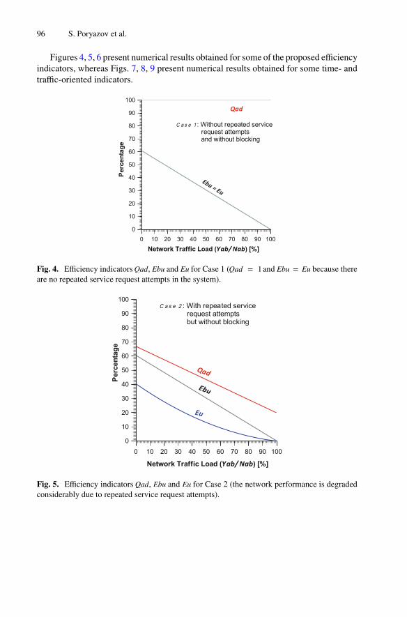
Figures 4, 5, 6 present numerical results obtained for some of the proposed efficiencyindicators, whereas Figs. 7, 8, 9 present numerical results obtained for some time- andtraffic-oriented indicators.

Fig. 4. Efficiency indicators Qad, Ebu and Eu for Case 1 (Qad = 1 and Ebu = Eu because thereare no repeated service request attempts in the system).

Fig. 5. Efficiency indicators Qad, Ebu and Eu for Case 2 (the network performance is degradedconsiderably due to repeated service request attempts).

96 S. Poryazov et al.

Fig. 6. Efficiency indicators Qad, Ebu and Eu for Case 3 (the network performance degradessharply due to blocking).

Fig. 7. Time and traffic AB-efficiency for Case 1 ((Ebu Tcc)∕Tab = (Eu Tcc)∕Tab, because thereare no repeated service request attempts).

Scalable Traffic Quality and System Efficiency Indicators 97

Fig. 8. Time and traffic AB-efficiency for Case 2 ((Eu Tcc) ∕Tab is sensitive to repeated servicerequest attempts in contrast to (Ebu Tcc) ∕Tab, which is not).

Fig. 9. Time and traffic AB-efficiency for Case 3 (the indicator paid Traffic ∕Yab is not sensibleenough in the network-load interval without blocking).

5 Network Cost/Quality Ratios

We consider the overall telecommunication system model, presented in Fig. 3, with thefollowing assumptions:

98 S. Poryazov et al.

Assumption 1: The observation time interval Δt is limited;Assumption 2: The full system costs (SC) in the time interval Δt are known;Assumption 3: The cost/quality ratio depends on the paid volume of traffic (paid.V) inthis time interval and the QoS indicator (Q);Assumption 4: The full system costs (SC) don’t depend considerably on the servedtraffic volume in the time interval Δt;Assumption 5: The QoS indicator (Q) is dimensionless with values from the interval(0,1] and is proportional to the quality (Q = 1 means ‘the best quality’).

5.1 Mean Cost/Quality Ratio

Based on these assumptions and the definition of the traffic volume, i.e. “The trafficvolume in a given time interval is the time integral of the traffic intensity over this timeinterval” [5], the ‘Cost per Unit’ quantity is:

Cost per Unit =Full System′s Costs [Euro]

Paid Traffic Volume [Erlang × Δt]. (56)

By dividing this to the QoS indicator (Q), we obtain the following:

Cost per Unit

Quality=

Full System′s Costs [Euro]

Q paid.V [Erlang × Δt]=

SC

Q paid.V. (57)

The definition of the paid traffic may depend on the telecommunication serviceprovider. The estimation of the paid traffic volume is a routine operation (c.f. ITU-TRecommendations Series D: General Tariff Principles).

The definition of the QoS indicator (Q) may differ from users’ perspective (i.e. as ageneralized QoE parameter) to the telecommunication service provider’s perspective.In general, the best is to include the Q definition in the Service Level Agreement (SLA).In any case, the value of the QoS indicator (Q) in (57) is the mean value in the timeinterval considered.

The mean cost/quality ratio (57) is suitable for relatively long intervals – days,months, years.

5.2 Instantaneous Cost/Quality Ratio

We consider the traffic intensity (Y) as per the ITU-T definition, i.e. “The instantaneoustraffic in a pool of resources is the number of busy resources at a given instant of time”[5]. From assumptions made and (57), the following formula could be obtained:

Cost per Unit

Quality=

Full System′s Costs [Euro]

Δt [Time] paid.Y [Erlang] Q=

SC

Δt Q paid.Y. (58)

The paid traffic intensity (paid.Y) is an instantaneous quantity but the ratio ‘Cost perUnit/Quality’ (58) depends on the time interval duration. We define the ‘System’s Costs

Scalable Traffic Quality and System Efficiency Indicators 99

Intensity’ (SCI) parameter, independent of the time interval duration (but dependent ofthe interval position in the service provider’s life time), as per the following formula:

System′s Costs Intensity (SCI) =Full System′s Costs [Euro]

Δt [Time]=

SC

Δt. (59)

The System’s Costs Intensity (SCI) parameter allows defining a new useful param‐eter – the Normalized Cost/Quality Ratio (NCQR):

Normalized Cost∕Quality Ratio (NCQR) =1

Q paid.Y [Erlang]. (60)

The Normalized Cost/Quality Ratio (NCQR) is independent of the absolute system’scosts amount. It is normalized, because it is the cost/quality ratio per 1 Euro cost.

From (57), (58), and (59), we obtain:

Cost per Unit

Quality=

Full System′s Costs [Euro]

Δt [Time]

1Q paid.Y [Erlang]

=

= SCI NCQR

(61)

The proposed quantities SCI and NCQR allow the estimation of the cost/quality ratiofor every suitable (paid) time interval with a relatively short duration, e.g. seconds,minutes, hours.

The paid traffic intensity depends on the network traffic load. In any case, the instan‐taneous values of the QoS indicator (Q) depend on many factors, including the networkload.

The expressions (57) and (58) are similar (the mean value of the instantaneous indi‐cator, in Δt, gives the value of the Mean Cost/Quality Ratio indicator in Δt), but themethods for their estimation and usage are different.

The Instantaneous Cost/Quality Ratio may be useful for dynamic pricing policies,depending on the network load. Related works on this subject were not found in theliterature.

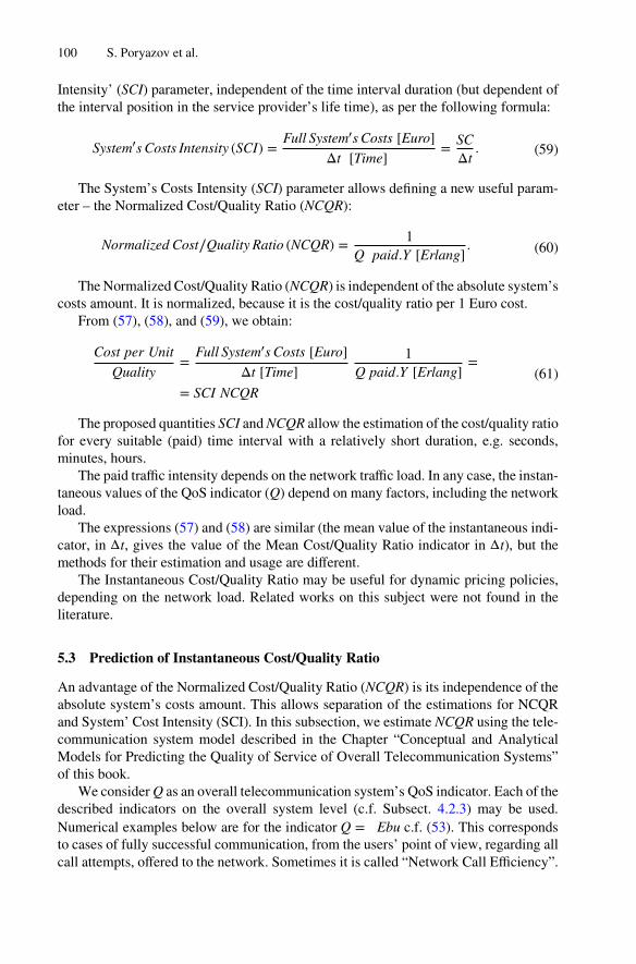
5.3 Prediction of Instantaneous Cost/Quality Ratio

An advantage of the Normalized Cost/Quality Ratio (NCQR) is its independence of theabsolute system’s costs amount. This allows separation of the estimations for NCQRand System’ Cost Intensity (SCI). In this subsection, we estimate NCQR using the tele‐communication system model described in the Chapter “Conceptual and AnalyticalModels for Predicting the Quality of Service of Overall Telecommunication Systems”of this book.

We consider Q as an overall telecommunication system’s QoS indicator. Each of thedescribed indicators on the overall system level (c.f. Subsect. 4.2.3) may be used.Numerical examples below are for the indicator Q = Ebu c.f. (53). This correspondsto cases of fully successful communication, from the users’ point of view, regarding allcall attempts, offered to the network. Sometimes it is called “Network Call Efficiency”.

100 S. Poryazov et al.

As a paid traffic, the successful communication (carried) traffic is used:

NCQR =1

Ebu paid.Y. (62)

The values of input parameters of human behavior and technical system, to themodel, in the presented output numerical results are typical for voice-oriented networks.

Figures 10 and 11 present numerical results for the entire theoretical network trafficload interval, i.e. the terminal traffic of all A- and B-terminals (Yab) is within the rangeof 0% to 100% of the number Nab of all active terminals in the system. The inputparameters are the same, excluding the capacity of the network (the number of equivalentconnection lines), given as a percentage of all terminals in the system. Differences inthe network capacity cause different blocking probabilities due to resource insufficiency.Two cases have been considered:

• Case 1: The network capacity equals 10% of all terminals presented in the system;• Case 2: The network capacity equals 25% of all terminals presented in the system.

Paid Network Traf f ic

0 10 20 30 40 50 60 70 80 90 100

0

10

20

30

40

50

60

70

80

Normalized C

ost /Qu

alityRatio

Network Traffic Load [%]

Call Eff iciency

NetworkCallE

fficiency(Ebu)[%]

Normalized

Cost/

QualityRatio

(NCQR)

[%]

Network capacity =10% of Terminals

Network

Fig. 10. Numerical prediction of the Normalized Cost/Quality Ratio (NCQR), Network CallEfficiency (Ebu), and Paid Traffic Intensity in an overall telecommunication system with QoSguarantees (Case 1: Network capacity = 10% of terminals).

Scalable Traffic Quality and System Efficiency Indicators 101

PaidNetw

orkTraf

f ic

0 10 20 30 40 50 60 70 80 90 100

0

10

20

30

40

50

60

70

80

Normalized

Cost /

QualityRatio

Network Traffic Load [%]

Network Call Efficiency

NetworkCallE

fficiency(Ebu

)[%]

Normalized

Cost/

QualityRati o

(NCQR)

[%] Network capacity =

25% of Terminals

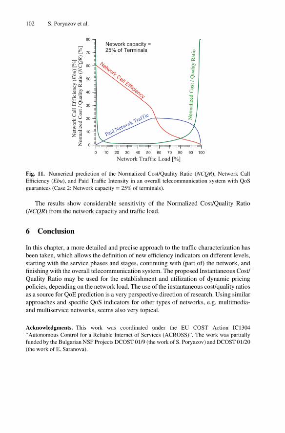
Fig. 11. Numerical prediction of the Normalized Cost/Quality Ratio (NCQR), Network CallEfficiency (Ebu), and Paid Traffic Intensity in an overall telecommunication system with QoSguarantees (Case 2: Network capacity = 25% of terminals).

The results show considerable sensitivity of the Normalized Cost/Quality Ratio(NCQR) from the network capacity and traffic load.

6 Conclusion

In this chapter, a more detailed and precise approach to the traffic characterization hasbeen taken, which allows the definition of new efficiency indicators on different levels,starting with the service phases and stages, continuing with (part of) the network, andfinishing with the overall telecommunication system. The proposed Instantaneous Cost/Quality Ratio may be used for the establishment and utilization of dynamic pricingpolicies, depending on the network load. The use of the instantaneous cost/quality ratiosas a source for QoE prediction is a very perspective direction of research. Using similarapproaches and specific QoS indicators for other types of networks, e.g. multimedia-and multiservice networks, seems also very topical.

Acknowledgments. This work was coordinated under the EU COST Action IC1304“Autonomous Control for a Reliable Internet of Services (ACROSS)”. The work was partiallyfunded by the Bulgarian NSF Projects DCOST 01/9 (the work of S. Poryazov) and DCOST 01/20(the work of E. Saranova).

102 S. Poryazov et al.

References

1. Reichl, P.: From charging for quality of service to charging for quality of experience. Ann.Telecommun. 65(3–4), 189–199 (2010)

2. Varela, M., Zwickl, P., Reichl, P., Xie, M., Schulzrinne, H.: From service level agreements(SLA) to experience level agreements (ELA): the challenges of selling QoE to the user. In:Proceedings of IEEE ICC QoE-FI, London, June 2015. ISSN: 2164-7038, https://doi.org/10.1109/iccw.2015.7247432

3. Fiedler, M.: Teletraffic models for quality of experience assessment. Tutorial at 23rdInternational Teletraffic Congress (ITC 23), San Francisco, CA, September 2011. http://iteletrafic.org/_Resources/Persistent/9269df1c3dca0bf58ee715c3b9afabbc71d4fb26/fiedler11.pdf. Accessed 20 July 2017

4. ITU-T Recommendation E.800 (09/08): Definitions of terms related to quality of service5. ITU-T Recommendation E.600 (03/93): Terms and definitions of traffic engineering6. Little, J.D.C.: A Proof of the Queueing Formula L = λW. Oper. Res. 9, 383–387 (1961)7. ITU-T Recommendation E.501(05/97): Estimation of Traffic Offered in The Network8. Poryazov, S., Saranova, E.: User-oriented, overall traffic and time efficiency indicators in

telecommunications. In: TELFOR 2016 International IEEE Conference #39555, Belgrade,Serbia, 22–23 November 2016, IEEE Catalog Number: CFP1698P-CDR. IEEE (2016). ISBN:978-1-5090-4086-5/16, INSPEC Accession Number: 16603129, https://doi.org/10.1109/telfor.2016.7818729

9. ITU-T Rec. E.425 (03/2002): Network management – Internal automatic observations

Open Access This chapter is licensed under the terms of the Creative Commons Attribution 4.0International License (http://creativecommons.org/licenses/by/4.0/), which permits use, sharing,adaptation, distribution and reproduction in any medium or format, as long as you give appropriatecredit to the original author(s) and the source, provide a link to the Creative Commons licenseand indicate if changes were made.

The images or other third party material in this chapter are included in the chapter’s CreativeCommons license, unless indicated otherwise in a credit line to the material. If material is notincluded in the chapter’s Creative Commons license and your intended use is not permitted bystatutory regulation or exceeds the permitted use, you will need to obtain permission directly fromthe copyright holder.

Scalable Traffic Quality and System Efficiency Indicators 103