MARINE ECOLOGY PROGRESS SERIESMar Ecol Prog Ser

Vol. 666: 57–72, 2021https://doi.org/10.3354/meps13683

Published May 20

1. INTRODUCTION

Saline and brackish marshes are vegetated ecosys-tems with specialized species that are adapted to livewithin the intertidal zone. These marshes provide

myriad ecosystem services, such as fisheries habitat(Barbier et al. 2011), protection of coasts from storms(Doughty et al. 2017), and carbon storage (Chmura etal. 2003, Ouyang & Lee 2013, Howard et al. 2017).The wetlands are vulnerable to direct degradation

© L.S.B., M.L., J.R., M.W., The Smithsonian, and (outside the USA)the US Governemnt 2021. Open Access under Creative Commonsby Attribution Licence. Use, distribution and reproduction are un -restricted. Authors and original publication must be credited.

Publisher: Inter-Research · www.int-res.com

*Corresponding author: holmquistj@si.edu

ABSTRACT: Elevation is a major driver of plant ecology and sediment dynamics in tidal wetlands,so accurate and precise spatial data are essential for assessing wetland vulnerability to sea-levelrise and making forecasts. We performed survey-grade elevation and vegetation surveys of theGlobal Change Research Wetland, a brackish microtidal wetland in the Chesapeake Bay estuary,Maryland (USA), to both intercompare unbiased digital elevation model (DEM) creation techniquesand to describe niche partitioning of several common tidal wetland plant species. We identified atradeoff between scalability and performance in creating unbiased DEMs, with more data-intensive methods such as kriging performing better than 3 more scalable methods involving post-processing of light detection and ranging (LiDAR)-based DEMs. The LiDAR Elevation Correctionwith Normalized Difference Vegetation Index (LEAN) method provided a compromise betweenscalability and performance, although it underpredicted variability in elevation. In areas where na-tive plants dominated, the sedge Schoenoplectus americanus occupied more frequently flooded ar-eas (median: 0.22, 95% range: 0.09 to 0.31 m relative to North America Vertical Datum of 1988[NAVD88]) and the grass Spartina patens, less frequently flooded (0.27, 0.1 to 0.35 m NAVD88).Non-native Phragmites australis dominated at lower elevations more than the native graminoids,but had a wide flooding tolerance, encompassing both their ranges (0.19, −0.05 to 0.36 m NAVD88).The native shrub Iva frutescens also dominated at lower elevations (0.20, 0.04 to 0.30 m NAVD88),despite being previously described as a high marsh species. These analyses not only provide valu-able context for the temporally rich but spatially restricted data collected at a single well-studiedsite, but also provide broad insight into mapping techniques and species zonation.

KEY WORDS: Brackish marsh · GCReW · Digital elevation model · Iva frutescens · LiDAR · Phragmites australis

OPENPEN ACCESSCCESS

Scalability and performance tradeoffs in quantifying relationships between elevation

and tidal wetland plant communities

James R. Holmquist1,*, Lisa Schile-Beers2, Kevin Buffington3, Meng Lu4, Thomas J. Mozdzer5, Jefferson Riera6, Donald E. Weller1, Meghan Williams1,

J. Patrick Megonigal1

1Smithsonian Environmental Research Center, Edgewater, MD 21403, USA2Silvestrum Climate Associates, LLC, San Francisco, CA 94102, USA

3US Geological Survey, Western Ecological Research Center, Vallejo, CA 93644, USA4Yunnan University, Kunming, PR China

5Bryn Mawr College, Bryn Mawr, PA 19010, USA6Johns Hopkins University, Baltimore, MD 21218, USA

Mar Ecol Prog Ser 666: 57–72, 202158

(Brophy et al. 2019), and their resilience or vulnera-bility to sea-level rise (SLR) is uncertain, althoughthey have some capacity to accrete in equilibriumwith SLR (Kirwan & Megonigal 2013). Vulnerabilityor resilience depends on a system’s capacity to cap-ture suspended sediment (Morris et al. 2002), theability of its plants to form soil mass by belowgroundroot addition (Nyman et al. 2006), and the spaceavailable for upslope transgression (Kirwan et al.2016).

Models used for forecasting marsh elevation’s dy -na mic response to SLR all require accurate ele -vation as an initial condition. These models includethe Marsh Equilibrium Model (MEM; Morris &Bowden 1986, Morris et al. 2002, 2016, Morris2006), MEM variations that include more detailedspatial analyses (Schile et al. 2014), Hydro-MEM(Alizad et al. 2016, 2018, Bacopoulos et al. 2019),Wetland Accretion Rate Model for Ecosystem Resil-ience (WARMER; Swanson et al. 2014, Thorne etal. 2018), models by Kirwan and Mudd (Kirwan &Mudd 2012), and the SLR Affecting Marshes Model(SLAMM; Park et al. 1989). Commonly used point-based models such as the MEM, WARMER, andKirwan-Mudd models also require information onplant tolerance to flooding, for which relative posi-tion in the tidal range is used as a proxy (Janouseket al. 2019). Small relative elevation changes canaffect phenomena such as vegetation zonationalong gradients as much as a few centimeters (Cas -tillo et al. 2000). Information to parameterize thesemodels comes from plants grown under controlledconditions at varying tidal elevations, so-calledmarsh organ experiments (Kirwan & Guntensper-gen 2015, Langley et al. 2013, Mozdzer et al. 2016),as well as high resolution GPS surveys of elevationand biomass (Schile et al. 2014) or plant presenceand absence (Thorne et al. 2018).

Monitoring multiple effects of global change ontidal wetland processes, including tidal elevation,has been a major focus of the Global Change Re -search Wetland (GCReW), located in KirkpatrickMarsh in the Chesapeake Bay estuary, Maryland(MD), USA. Various wetland grasses (C4), sedges(C3), and the invasive Phragmites australis (Cav.)Trin. ex Steud have been the subject of studiesinvestigating the physiological tolerances andniches of species using experimental, marsh organ-style, floo ding treatments at GCReW (Langley etal. 2013, Mozdzer et al. 2016). GCReW has notyet had an extensive elevation survey (Nelson etal. 2017), which limits the ability to verify thatthe modern elevations represented in the marsh

organ experiments are representative of the land-scape.

The most scalable techniques for producing digi-tal elevation models (DEMs) use light detectionand ranging (LiDAR); however, LiDAR data areprone to bias in tidal wetlands because laserpulses often do not fully penetrate low, dense veg-etation or standing dead biomass and because wetsoil can absorb some light, leading to obfuscatedreturns after post- processing (Hladik et al. 2013,Medeiros et al. 2015, Buffington et al. 2016). Thesebiases yield modeled elevations that are higherthan those measured using ground-based techniques.Elevation errors are particularly problematic incoastal wetland systems since subtle vari ations inelevation result in different plant communities andfunctions (Alizad et al. 2020).

There are methods for generating unbiased wet-land DEMs which range in complexity from simpleadjustments based on height to data-intensive statis-tical correction models. For a national scale assess-ment, Holmquist et al. (2018) corrected the elevationbias by subtracting a single average offset estimatedfrom a literature review, for a contiguous USA-wideprobabilistic area estimate of coastal lands. This sin-gle offset approach did not account for spatial varia-tion in the bias term, so national-scale products couldbe enhanced with more localized analysis. Some stu -dies correct elevation zones using maps of vegetationcommunity distribution (Hladik et al. 2013, Schile etal. 2014). Buffington et al. (2016) applied a multivari-ate linear regression to correct bias in tidal wetlandsusing the LiDAR elevation estimate and the Normal-ized Difference of Vegetation Index (NDVI), a meas-ure of vegetation greenness mapped from NationalAgriculture Imagery Program (NAIP) imagery. Thismethod is called the LiDAR Elevation Adjustmentusing NDVI (LEAN) algorithm. Other studies haveavoided LiDAR altogether, instead spatially interpo-lating a 3-dimensional surface among point-basedsurveys (Thorne et al. 2013, 2018). While such sur-veys are essential for sea-level resiliency assess-ments, more extensive field-based collection of ele-vation data is costly and damages sensitive sites, sothere is a need for techniques that can be appliedacross larger areas with a minimal number of calibra-tion points.

Furthermore, despite the intensive, long-termexperiments at GCReW, no previous study has docu-mented the natural history of important vegetation−elevation relationships at the site. Previous studieshave focused on 3 major communities that domi-nated the site when experiments were first started in

Holmquist et al.: Tidal elevation and wetland communities

1987. Schoenoplectus americanus (Pers.) Volkart exSchinz & R. Keller (formerly Scirpus olneyi) occupiesmore frequently inundated portions of the marsh anda C4 grass mix of Distichlis spicata (L.) Greene, andSpartina patens (Aiton) Muhl. dominates less fre-quently inundated portions of the marsh. Marshorgan experiments at GCReW have been able to con-strain a minimum and maximum elevation tolerancefor S. americanus, but have not constrained theupper growing limit for C4 grasses (Langley et al.2013). This lack of a documented upper limit forhigh-marsh grasses is not unique to GCReW; it hasalso been observed for marshes on the opposite shoreof Chesapeake Bay along Blackwater Bay, MD (Kir-wan & Guntenspergen 2015). An invasive lineage ofthe common reed P. australis dominates major areasof the site. This species has been present in the mid-Atlantic since before 1910 and has expanded greatlysince the 1960s (Rice et al. 2000, Saltonstall 2002),expanding its area at GCReW 22-fold since 1972(McCormick et al. 2010). Documenting the relation-ships between elevation and P. australis dominancecould provide insight into its status as an invasivespecies, as well as provide information on how it mayaffect marshes in the future. Finally, there are farmore than 3 species present at the marsh. For exam-ple, the native shrub Iva frutescens L. has not beenintegrated into any global change experiments de -spite being a dominant component of common vege-tation communities at GCReW (Byrd et al. 2018).

Given that there are multiple methods for creatingunbiased DEMs with differing levels of data require-ments, and that the extensive experimental data atGCReW need site-wide elevation to add context toand provide comparison for marsh organ studies, ourgoals were 3-fold. First, to survey elevation and rela-tive plant cover of the entire marsh complex at 20 ×20 m resolution and to document the distribution ofelevation relative to tidal datums from a single year.Second, to use these elevation data to generate 4 dif-ferent unbiased DEMs utilizing different techniques,then assess their accuracies and precisions andquantify the tradeoffs between performance andscalability. We hypothesized that there would be atradeoff between scalability and performance, withmore labor-intensive methods providing better per-formance. Third, to quantify wetland plant presenceand relative dominance in terms of observed eleva-tion/inundation niches for different plant species. Wehypothesized that dominant plant communities parti-tion elevation niches, with S. americanus being loca -ted in more frequently flooded areas and C4 grasseslocated in less frequently flooded areas.

2. MATERIALS AND METHODS

2.1. Site description

GCReW is located at the Smithsonian Environ-mental Research Center in Edgewater, MD, USA.The site is one of the most studied tidal wetlandsin the world and is the source of many impactfulinsights on relationships among plant traits, micro-bial activity, and soil biogeochemical responses toglobal change factor interactions. GCReW occupiesabout half of a larger 22 ha marsh complex knownlocally as Kirkpatrick Marsh (Fig. 1). The site hasbeen commonly referred to as a high marsh (Lang-ley et al. 2013, Lu et al. 2019), but this status as ahigh marsh has not been explicitly quantified rela-tive to tidal flooding across the whole site. The siteis brackish throughout the year but has seasonaland interannual variance in salinity due to fresh-water input from precipitation. The system is mi -crotidal, with a greater diurnal tidal range of0.44 m, as measured at a nearby tide gauge inAnna polis, MD (NOAA 2020a) over the last datumperiod (1983− 2001). In the Chesapeake Bay, rela-tive SLR was 3.67 ± 0.20 mm yr−1 from 1928−2019(NOAA 2020b). A portion of this is eustatic SLR,and a portion is attributable to subsidence, 1.3−1.5mm yr−1 in the region according to GPS (Karegaret al. 2016). The climate zone is classified as tem-perate with no dry season and hot summers.

2.2. Tidal datum transformations

We summarized elevation data relative to tidaldatums that were calculated from the nearby Anna -polis tidal gauge located 13 km from GCReW. Wecalculated a suite of tidal datums for 2016 from com-plete, verified, 6 min tide gauge data. We used the‘ftide’ function in the R package ‘tideharmonics’(Stephenson 2016) to calculate a set of 60 harmonicconstituents. We then predicted tides at the same6 min resolution as the data using nearest neighboranalysis to isolate high and low tides, then differenti-ated higher high tides from lower high tides, andlower low tides from higher low tides. We used a 52tide moving window and reclassified the highesthigh tide as spring higher high water and the lowestpredicted tide of the lunar period as the lower lowspring tide.

We calculated mean sea level (MSL), highest ob -served tide (HOT), and lowest observed tide (LOT)by calculating the mean, minimum, and maximum of

59

Mar Ecol Prog Ser 666: 57–72, 2021

the observed data set. We calculated mean highwater (MHW), mean higher high water (MHHW),mean higher high water spring tides (MHHWS),mean low water (MLW), mean lower low water(MLLW), and mean lower low water spring tides(MLLWS) by taking the average water levels of theclassified predicted water levels. We quantified thehighest and lowest astronomical tide (HAT and LAT)from the minimum and maximum of the predictedwater levels.

2.3. Improvements to geodetic control network

We strengthened the geodetic control networkproperty-wide by performing 4 long occupations offixed monuments with JAVAD company total stationGPS units, one of which was used as the base sta-tion for the current study. Two of these occupationswere done on geodetic markers on the north side ofthe Rhode River on monuments installed by theNational Geodetic Survey and the SmithsonianInstitution. For the 2 survey-grade monuments onthe north side of the Rhode River, GPS units were

mounted on a 2 m tripod on a 0.25 m adapter with a0.025 m attachment.

In wetlands, soil elevation is prone to dynamicchanges because of sediment consolidation, expan-sion of the rooting zone by root growth, and contrac-tion of the rooting zone by soil organic matter decom-position. Therefore, geodetic monuments need to beattached to rods driven several meters into theground, hitting bedrock (Cahoon et al. 2002). AtGCReW, we occupied 2 such deep-rod monuments,one near a tidal creek near a flume and marsh organexperiments, and the other closer to the upland inter-face near the sediment elevation table (SET) used tomonitor net-elevation change in an experimentalplot (Langley et al. 2009). For the flume location, thetotal station GPS unit was mounted on a 1.5 m tripodwith a 0.25 m adapter and a 0.025 m attachment. Theequipment was centered on the monument on apointed tip and was leveled using a bubble levelbuilt into the tripod. At one SET (referred to as SET#17 in the supplemental data release; Holmquist etal. 2021), the unit was mounted on a 2 m survey-grade pole and a 0.025 m attachment. Instead ofbeing centered on a monument point, it was screwed

60

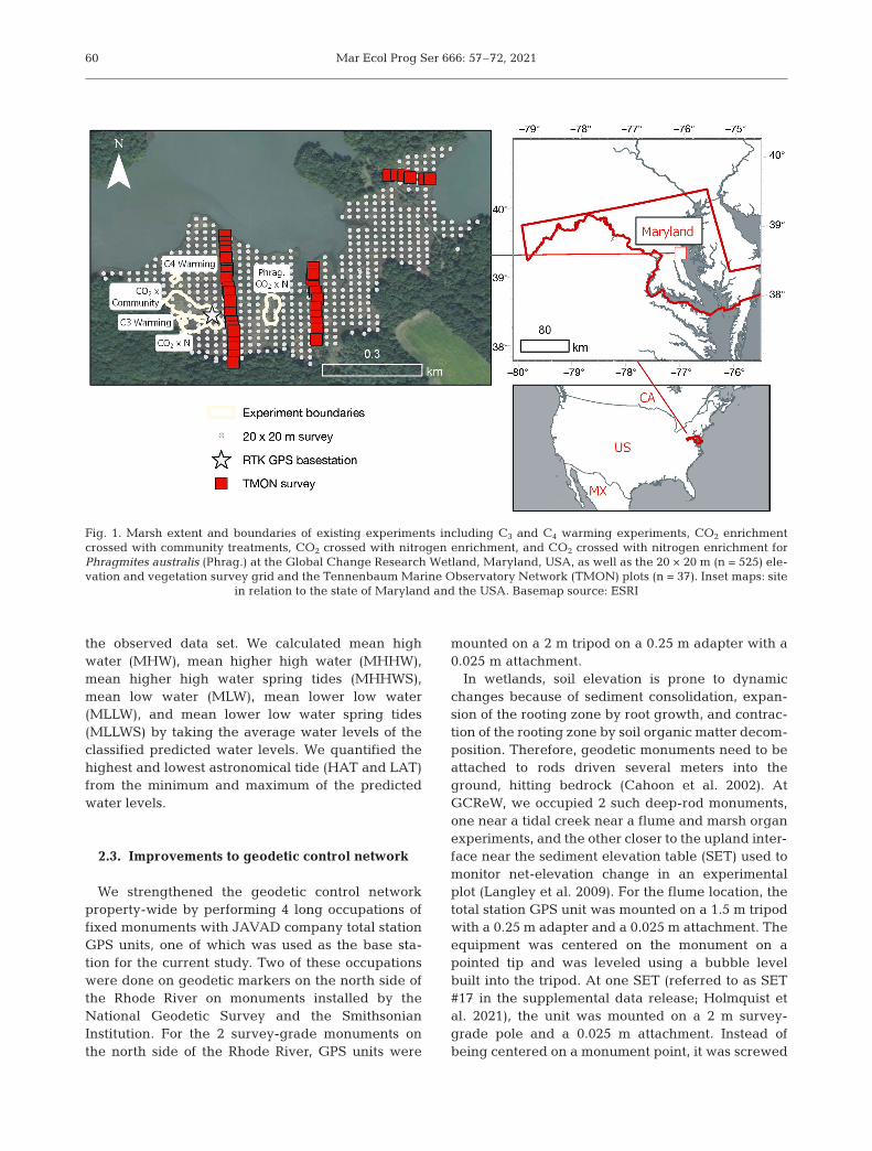
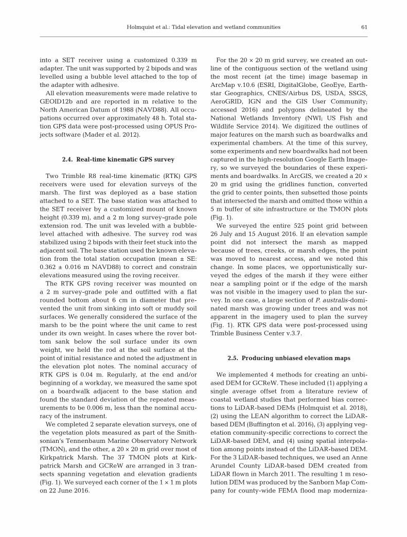
Fig. 1. Marsh extent and boundaries of existing experiments including C3 and C4 warming experiments, CO2 enrichmentcrossed with community treatments, CO2 crossed with nitrogen enrichment, and CO2 crossed with nitrogen enrichment forPhragmites australis (Phrag.) at the Global Change Research Wetland, Maryland, USA, as well as the 20 × 20 m (n = 525) ele-vation and vegetation survey grid and the Tennenbaum Marine Observatory Network (TMON) plots (n = 37). Inset maps: site

in relation to the state of Maryland and the USA. Basemap source: ESRI

Holmquist et al.: Tidal elevation and wetland communities

into a SET receiver using a customized 0.339 madapter. The unit was supported by 2 bipods and waslevelled using a bubble level attached to the top ofthe adapter with adhesive.

All elevation measurements were made relative toGEOID12b and are reported in m relative to theNorth American Datum of 1988 (NAVD88). All occu-pations occurred over approximately 48 h. Total sta-tion GPS data were post-processed using OPUS Pro-jects software (Mader et al. 2012).

2.4. Real-time kinematic GPS survey

Two Trimble R8 real-time kinematic (RTK) GPSreceivers were used for elevation surveys of themarsh. The first was deployed as a base stationattached to a SET. The base station was attached tothe SET receiver by a customized mount of knownheight (0.339 m), and a 2 m long survey-grade poleextension rod. The unit was leveled with a bubble-level attached with adhesive. The survey rod wasstabilized using 2 bipods with their feet stuck into theadjacent soil. The base station used the known eleva-tion from the total station occupation (mean ± SE:0.362 ± 0.016 m NAVD88) to correct and constrainelevations measured using the roving receiver.

The RTK GPS roving receiver was mounted ona 2 m survey-grade pole and outfitted with a flatrounded bottom about 6 cm in diameter that pre-vented the unit from sinking into soft or muddy soilsurfaces. We generally considered the surface of themarsh to be the point where the unit came to restunder its own weight. In cases where the rover bot-tom sank below the soil surface under its ownweight, we held the rod at the soil surface at thepoint of initial resistance and noted the adjustment inthe elevation plot notes. The nominal accuracy ofRTK GPS is 0.04 m. Regularly, at the end and/orbeginning of a workday, we measured the same spoton a boardwalk adjacent to the base station andfound the standard deviation of the repeated meas-urements to be 0.006 m, less than the nominal accu-racy of the instrument.

We completed 2 separate elevation surveys, one ofthe vegetation plots measured as part of the Smith-sonian’s Tennenbaum Marine Observatory Network(TMON), and the other, a 20 × 20 m grid over most ofKirkpatrick Marsh. The 37 TMON plots at Kirk-patrick Marsh and GCReW are arranged in 3 tran-sects spanning vegetation and elevation gradients(Fig. 1). We surveyed each corner of the 1 × 1 m plotson 22 June 2016.

For the 20 × 20 m grid survey, we created an out-line of the contiguous section of the wetland usingthe most recent (at the time) image basemap inArcMap v.10.6 (ESRI, DigitalGlobe, GeoEye, Earth-star Geographics, CNES/Airbus DS, USDA, SSGS,AeroGRID, IGN and the GIS User Community;accessed 2016) and polygons delineated by theNational Wetlands Inventory (NWI; US Fish andWildlife Service 2014). We digitized the outlines ofmajor features on the marsh such as boardwalks andexperimental chambers. At the time of this survey,some experiments and new boardwalks had not beencaptured in the high-resolution Google Earth Ima ge -ry, so we surveyed the boundaries of these experi-ments and boardwalks. In ArcGIS, we created a 20 ×20 m grid using the gridlines function, convertedthe grid to center points, then subsetted those pointsthat intersected the marsh and omitted those within a5 m buffer of site infrastructure or the TMON plots(Fig. 1).

We surveyed the entire 525 point grid between26 July and 15 August 2016. If an elevation samplepoint did not intersect the marsh as mappedbecause of trees, creeks, or marsh edges, the pointwas moved to nearest access, and we noted thischange. In some places, we opportunistically sur-veyed the edges of the marsh if they were eithernear a sampling point or if the edge of the marshwas not visible in the imagery used to plan the sur-vey. In one case, a large section of P. australis-domi-nated marsh was growing under trees and was notapparent in the imagery used to plan the survey(Fig. 1). RTK GPS data were post-processed usingTrimble Business Center v.3.7.

2.5. Producing unbiased elevation maps

We implemented 4 methods for creating an unbi-ased DEM for GCReW. These included (1) applying asingle average offset from a literature review ofcoastal wetland studies that performed bias correc-tions to LiDAR-based DEMs (Holmquist et al. 2018),(2) using the LEAN algorithm to correct the LiDAR-based DEM (Buffington et al. 2016), (3) applying veg-etation community-specific corrections to correct theLiDAR-based DEM, and (4) using spatial interpola-tion among points instead of the LiDAR-based DEM.For the 3 LiDAR-based techniques, we used an AnneArundel County LiDAR-based DEM created fromLiDAR flown in March 2011. The resulting 1 m reso-lution DEM was produced by the Sanborn Map Com-pany for county-wide FEMA flood map moderniza-

61

Mar Ecol Prog Ser 666: 57–72, 2021

tion. The LiDAR flight and our RTK GPS survey were4 yr apart, but we assumed that any accretion or sub-sidence over that time would be within the nominalerror of the RTK GPS.

We used the LEAN technique to correct the verti-cal bias in LiDAR-based DEMs due to dense vegeta-tion coverage (Buffington et al. 2016). LEAN usesground measurements of elevation, typically fromRTK GPS, to calculate the vertical bias in LiDAR datasets. Initial LiDAR elevation and the NDVI ( = [NIR −Red] / [NIR + Red]; red wavelength = 608−662 nm,near infrared [NIR] wavelengths = 833−887 nm) fromNAIP were used in a multivariate linear regressionmodel to estimate the bias. NDVI was assumed to bea metric of vegetation height and density. We usedall RTK GPS marsh elevation points from the 20 mgrid survey to calibrate LEAN. The 4 band NAIPimagery used to calculate NDVI was acquired24 July 2015. To estimate model skill, we used a 10-fold cross validation procedure in which the modelwas iteratively fit with 90% of the elevation data andtested against the 10% hold out.

We used a digitized map of GCReW vegetationzones to test applying cover-based elevation bias corrections. The map we used consists of the 6major vegetation cover types: an Iva frutescens-dominated community, I. frutescens and Phrag-mites australis mixed community, a Schoenoplectusamericanus and Spartina patens mixed community,a P. australis- dominated community, a S. ameri-canus-dominated community, and a S. patens-dominated community. Community boundarieswere delineated by trained personnel using high-resolution 2010 summer image ry in Google Earth.Polygons were assigned one of 6 vegetation typesusing the interactive supervised classification toolin ArcGIS which uses the maximum likelihoodmethod, trained using 26 total ground-based ref-erence points that were collected in 2014. Thismap, created for a separate unpublished project,and the associated data release (Lu & Williams2021) compares the vegetation communities in2010 to those delineated from an image taken in1973 (Jenkens 1973).

We used ANOVA to test if there were significantdifferences between measured and uncorrectedmapped LiDAR-based elevation from the 20 m gridsurvey, using the mapped vegetation community inthe 2010 map as an independent variable and LiDARoffset as the dependent variable. If the relationshipwas significant, then we could create a new DEM bysubtracting those vegetation offsets from the mappedsurface.

We performed empirical Bayesian kriging usingArcGIS Pro v.2.4 applied to all marsh surface datafrom the 20 m grid survey. We mapped both themedian prediction and standard error of the krigedsurface using a power semivariogram and a 100 max-imum point standard circular neighborhood with aradius of 272 m.

2.6. Intercomparing unbiased elevation mapping strategies

We compared the 4 techniques by validating eachof the 4 maps with the TMON elevation plot meas-urements, which were independent of all vegetationheight correction strategies. We calculated the biasas mean error and precision as unbiased root meansquare error (RMSE’). We normalized both of thesemetrics (shown by *) to the standard deviation of thereference data set (σr). We also calculated the totalRMSE, the sum of squares of mean error and RMSE’.Normalized total RMSE (RMSE*) provides a con -venient performance threshold. When a strategy’sRMSE* is less than 1, it performs better than simplyapplying the average from the reference data set(Jolliff et al. 2009). We then ranked the 4 strategiesbased on our interpretation of their scalability, mean-ing the feasibility of applying the strategy to differentsites with a larger extent.

2.7. Vegetation survey

In conjunction with the grid-based elevation sur-vey, we also recorded plant community presence,absence, and relative abundance. At each elevationplot, we estimated ordinal Braun-Blanquet scores formajor vegetation community types (Braun-Blanquet1932, Snedden & Steyer 2013). The area of the esti-mation was approximately a 1 m circumference cir-cle around the center of the elevation point estimatedas the length of the extended arm of the technicianrecording elevation and vegetation. Braun-Blanquetscores ranged from 0−5, with 0 indicating traceamounts of cover (<1% of the aerial view of the plot);1 = 1−5%; 2 = 5−25%; 3 = 25−50%; 4 = 50−75%; and5 = 75−100%. The major communities we recordedincluded S. americanus, the C4 mix of Distichlis spi-cata and S. patens, the shrub I. frutescens, and theinvasive reed P. australis. We recorded minor plantspecies as well. To enhance consistency, the sametechnician recorded all elevation and vegetationmeasurements.

62

Holmquist et al.: Tidal elevation and wetland communities

2.8. Data analyses and statistics

Data were analyzed in R v.3.5.3 (R Core Team2019). We performed dataframe manipulations using‘dplyr’ (Wickham et al. 2019) and ‘lubridate’ (Grole-mund & Wickham 2011). Moving window time-seriesanalysis was performed using ‘zoo’ (Zeileis & Gro -then dieck 2005). Graphs were made using ‘ggplot’(Wickham 2016) and ‘gridExtra’ (Auguie 2017). Mapswere created using ‘ggmap’ (Kahle & Wickham 2013)in R, except for Fig. 1 which was made using ArcGISPro.

3. RESULTS

3.1. Tidal datums for 2016

The full suite of tidal datums calculated for 2016from the Annapolis tide gauge are listed in Table 1.The MSL was 0.092 m. Other tidal datums wereas follows: MHW = 0.194 m NAVD88, MHHW =0.278 m, and MHHWS = 0.340 m. Observed waterlevels ranged from −0.847 to 0.861 m.

3.2. Elevation distribution of the GCReW

Summary statistics of the elevation distributionmeasured in the 20 m grid survey are presented inTable 2. The elevation gradient surveyed at GCReWranged from −0.247 to 0.444 m. Mean (±SD) eleva-tion was 0.209 ± 0.092 m. The distribution of eleva-

63

Datum Elevation (m)(NAVD88)

Highest observed tide 0.861Highest astronomical tide 0.500Mean higher high water spring 0.340Mean higher high water 0.278Mean high water 0.194Mean sea level 0.092Mean low water −0.007Mean lower low water −0.088Mean lower low water spring −0.096Lowest astronomical tide −0.336Lowest observed tide −0.847

Table 1. Tidal datums at the 2016 Annapolis tide gauge (NAVD88, North American Vertical Datum of 1988)

Analysis Cover n Mean SD Min. 2.5% 25% Median 75% 97.5% Max.

Total elevation NA 523 0.209 0.092 −0.247 −0.028 0.160 0.221 0.274 0.351 0.444Presence SCAM 308 0.219 0.075 −0.191 0.066 0.174 0.231 0.274 0.325 0.363Presence C4 293 0.234 0.075 −0.191 0.08 0.195 0.247 0.286 0.337 0.444Presence IVFR 230 0.203 0.082 −0.051 0.020 0.151 0.214 0.265 0.326 0.353Presence PHAU 224 0.195 0.092 −0.119 −0.025 0.149 0.200 0.254 0.358 0.444Presence SPCY 61 0.188 0.113 −0.078 −0.040 0.116 0.191 0.262 0.366 0.406Presence KOVI 57 0.217 0.070 0.081 0.092 0.169 0.219 0.261 0.346 0.376Presence TYLA 29 0.221 0.069 0.081 0.103 0.173 0.220 0.274 0.339 0.352Presence SOSE 14 0.268 0.064 0.092 0.132 0.231 0.292 0.304 0.333 0.340Presence SPAL 11 0.166 0.105 −0.032 0.001 0.114 0.146 0.224 0.328 0.329Presence AMAR 9 0.175 0.132 −0.104 −0.064 0.146 0.168 0.304 0.316 0.318Presence HIMO 7 0.221 0.153 −0.104 −0.058 0.217 0.232 0.327 0.332 0.333Dominance C4 160 0.255 0.066 −0.032 0.10 0.231 0.270 0.301 0.353 0.363Dominance PHAU 153 0.182 0.096 −0.119 −0.053 0.131 0.191 0.235 0.362 0.444Dominance IVFR 126 0.192 0.074 −0.040 0.036 0.144 0.199 0.244 0.306 0.325Dominance SCAM 119 0.214 0.070 −0.191 0.087 0.184 0.222 0.260 0.305 0.336Dominance SPCY 19 0.206 0.13 −0.040 −0.038 0.140 0.205 0.320 0.393 0.406Dominance TYLA 15 0.242 0.064 0.113 0.129 0.210 0.245 0.282 0.346 0.352Dominance KOVI 9 0.208 0.076 0.093 0.099 0.155 0.204 0.278 0.308 0.315Dominance SPAL 4 0.136 0.055 0.098 0.098 0.103 0.114 0.148 0.209 0.216

Table 2. Summary statistics of elevation distribution measured for total elevation, vegetation type presences, and vegetationtype dominance. Study site is the Global Change Research Wetland and Kirkpatrick Marsh in Edgewater, Maryland, USA(38° 52’ 29’’ N, 76° 32’ 48’’ W). Ground survey data was collected between 26 July and 15 August 2016. Statistics include thenumber of observations (n), and the 2.5, 25, 75, and 97.5% quantiles. Cover types include Schoenoplectus americanus(SCAM), C4 grasses Spartina patens and Distichlis spicata, Iva frutescens (IVFR), Phragmites australis (PHAU), Spartina cyno-suroides (SPCY), Kosteletzkya virginica (KOVI), Typha latifolia (TYLA), Solidago sempervirens (SOSE), Spartina alterniflora(SPAL), Amaranthus cannabinus (AMAR), and Hibiscus moscheutos (HIMO). Statistics were summarized for all plots wherespecies were present (Presence), and all plots where the species was the dominant, or co-dominant cover type (Dominance)

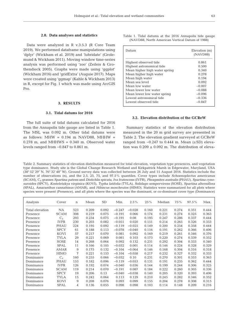
tion centered around its median (0.221 m NAVD88),which skewed higher than its mean (Fig. 2). Overall,the distribution had a positive skew with a long tailon the lower end of the elevation gradient.

We classified the elevation survey points accordingto regularity of tidal flooding at different levels. Wefound that 37.1% of the marsh was below the MHWline (Fig. 2), receiving semidiurnal tides. We classi-fied the majority of the marsh concentrated betweenthe MHHW and MHW water lines (40.5%) as beinginundated once per day. About one-fifth (19.7%) ofthe marsh was between the MHHWS and MHHWlines, being inundated once daily to twice a month.The remaining 2.7% was classified as above theMHHWS line.

3.3. Digital elevation mapping

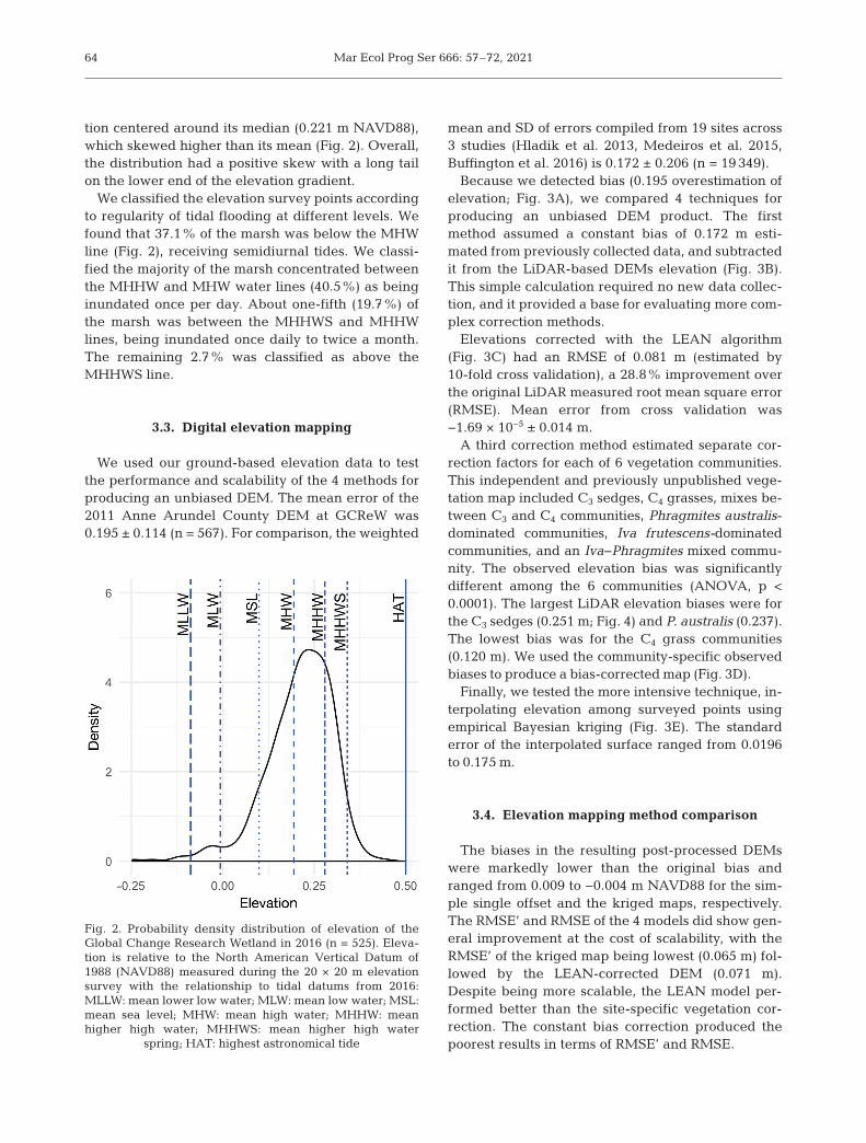
We used our ground-based elevation data to testthe performance and scalability of the 4 methods forproducing an unbiased DEM. The mean error of the2011 Anne Arundel County DEM at GCReW was0.195 ± 0.114 (n = 567). For comparison, the weighted

mean and SD of errors compiled from 19 sites across3 studies (Hladik et al. 2013, Medeiros et al. 2015,Buffington et al. 2016) is 0.172 ± 0.206 (n = 19 349).

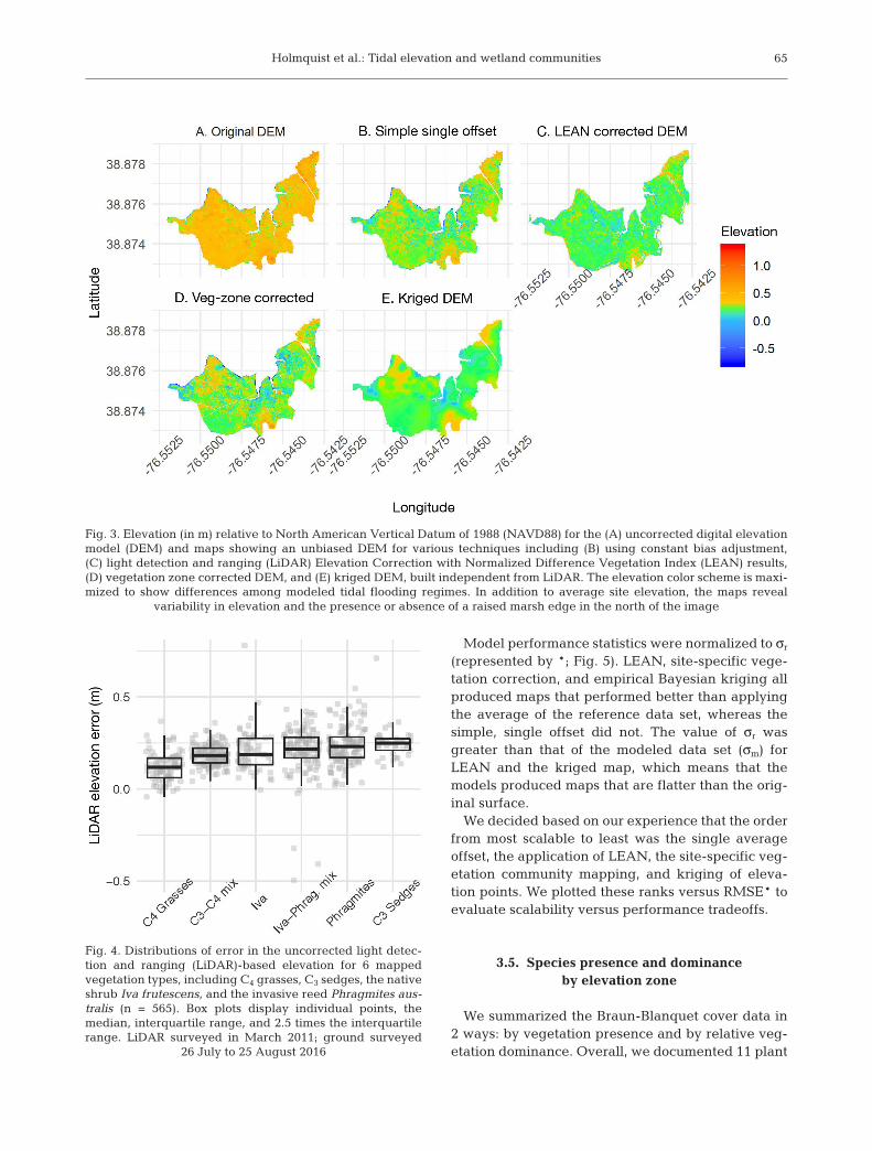
Because we detected bias (0.195 overestimation ofelevation; Fig. 3A), we compared 4 techniques forproducing an unbiased DEM product. The firstmethod assumed a constant bias of 0.172 m esti-mated from previously collected data, and subtractedit from the LiDAR-based DEMs elevation (Fig. 3B).This simple calculation required no new data collec-tion, and it provided a base for evaluating more com-plex correction methods.

Elevations corrected with the LEAN algorithm(Fig. 3C) had an RMSE of 0.081 m (estimated by10-fold cross validation), a 28.8% improvement overthe original LiDAR measured root mean square error(RMSE). Mean error from cross validation was−1.69 × 10−5 ± 0.014 m.

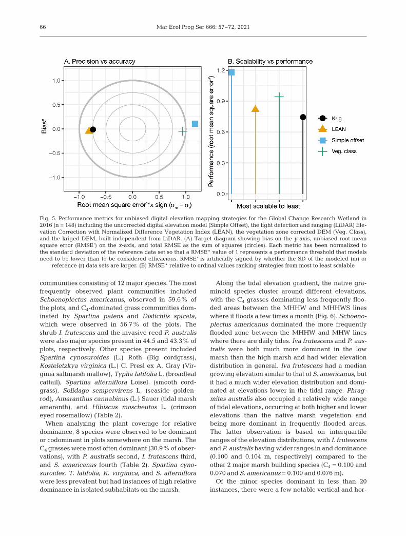
A third correction method estimated separate cor-rection factors for each of 6 vegetation communities.This independent and previously unpublished vege-tation map included C3 sedges, C4 grasses, mixes be -tween C3 and C4 communities, Phragmites australis-dominated communities, Iva frutescens-dominatedcommunities, and an Iva−Phragmites mixed commu-nity. The observed elevation bias was significantlydifferent among the 6 communities (ANOVA, p <0.0001). The largest LiDAR elevation biases were forthe C3 sedges (0.251 m; Fig. 4) and P. australis (0.237).The lowest bias was for the C4 grass communities(0.120 m). We used the community-specific observedbiases to produce a bias-corrected map (Fig. 3D).

Finally, we tested the more intensive technique, in-terpolating elevation among surveyed points usingempirical Bayesian kriging (Fig. 3E). The standard error of the interpolated surface ranged from 0.0196to 0.175 m.

3.4. Elevation mapping method comparison

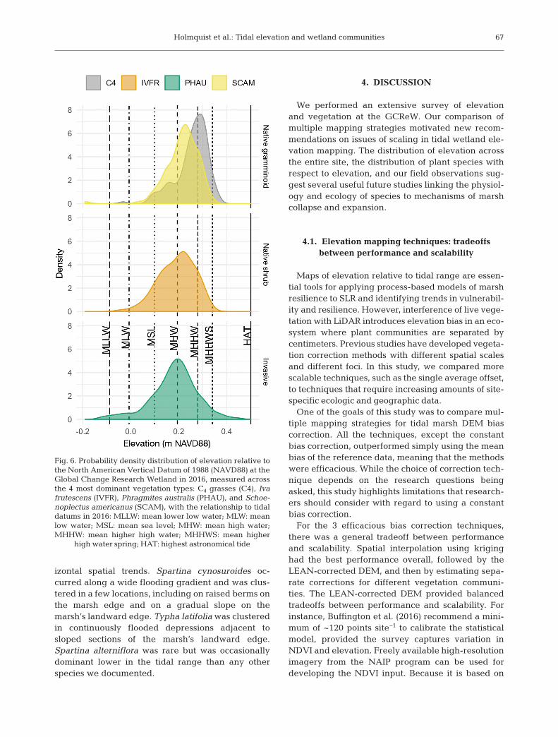
The biases in the resulting post-processed DEMswere markedly lower than the original bias andranged from 0.009 to −0.004 m NAVD88 for the sim-ple single offset and the kriged maps, respectively.The RMSE’ and RMSE of the 4 models did show gen-eral improvement at the cost of scalability, with theRMSE’ of the kriged map being lowest (0.065 m) fol-lowed by the LEAN-corrected DEM (0.071 m).Despite being more scalable, the LEAN model per-formed better than the site-specific vegetation cor-rection. The constant bias correction produced thepoorest results in terms of RMSE’ and RMSE.

Mar Ecol Prog Ser 666: 57–72, 202164

Fig. 2. Probability density distribution of elevation of theGlobal Change Research Wetland in 2016 (n = 525). Eleva-tion is relative to the North American Vertical Datum of1988 (NAVD88) measured during the 20 × 20 m elevationsurvey with the relationship to tidal datums from 2016:MLLW: mean lower low water; MLW: mean low water; MSL:mean sea level; MHW: mean high water; MHHW: meanhigher high water; MHHWS: mean higher high water

spring; HAT: highest astronomical tide

Holmquist et al.: Tidal elevation and wetland communities

Model performance statistics were normalized to σr

(represented by *; Fig. 5). LEAN, site-specific vege-tation correction, and empirical Bayesian kriging allproduced maps that performed better than applyingthe average of the reference data set, whereas thesimple, single offset did not. The value of σr wasgreater than that of the modeled data set (σm) forLEAN and the kriged map, which means that themodels produced maps that are flatter than the orig-inal surface.

We decided based on our experience that the orderfrom most scalable to least was the single averageoffset, the application of LEAN, the site-specific veg-etation community mapping, and kriging of eleva-tion points. We plotted these ranks versus RMSE* toevaluate scalability versus performance tradeoffs.

3.5. Species presence and dominance by elevation zone

We summarized the Braun-Blanquet cover data in2 ways: by vegetation presence and by relative veg-etation dominance. Overall, we documented 11 plant

65

Fig. 3. Elevation (in m) relative to North American Vertical Datum of 1988 (NAVD88) for the (A) uncorrected digital elevationmodel (DEM) and maps showing an unbiased DEM for various techniques including (B) using constant bias adjustment,(C) light detection and ranging (LiDAR) Elevation Correction with Normalized Difference Vegetation Index (LEAN) results,(D) vegetation zone corrected DEM, and (E) kriged DEM, built independent from LiDAR. The elevation color scheme is maxi -mized to show differences among modeled tidal flooding regimes. In addition to average site elevation, the maps reveal

variability in elevation and the presence or absence of a raised marsh edge in the north of the image

Fig. 4. Distributions of error in the uncorrected light detec-tion and ranging (LiDAR)-based elevation for 6 mappedvegetation types, including C4 grasses, C3 sedges, the nativeshrub Iva frutescens, and the invasive reed Phragmites aus-tralis (n = 565). Box plots display individual points, themedian, interquartile range, and 2.5 times the interquartilerange. LiDAR surveyed in March 2011; ground surveyed

26 July to 25 August 2016

communities consisting of 12 major species. The mostfrequently observed plant communities includedSchoenoplectus americanus, observed in 59.6% ofthe plots, and C4-dominated grass communities dom-inated by Spartina patens and Distichlis spicata,which were observed in 56.7% of the plots. Theshrub I. frutescens and the invasive reed P. australiswere also major species present in 44.5 and 43.3% ofplots, respectively. Other species present includedSpartina cynosuroides (L.) Roth (Big cordgrass),Kosteletzkya virginica (L.) C. Presl ex A. Gray (Vir-ginia saltmarsh mallow), Typha latifolia L. (broadleafcattail), Spartina alterniflora Loisel. (smooth cord-grass), Solidago sempervirens L. (seaside golden-rod), Amaranthus cannabinus (L.) Sauer (tidal marshamaranth), and Hibiscus moscheutos L. (crimsoneyed rosemallow) (Table 2).

When analyzing the plant coverage for relativedominance, 8 species were observed to be dominantor codominant in plots somewhere on the marsh. TheC4 grasses were most often dominant (30.9% of obser-vations), with P. australis second, I. frutescens third,and S. americanus fourth (Table 2). Spartina cyno-suroides, T. latifolia, K. virginica, and S. alterniflorawere less prevalent but had instances of high relativedominance in isolated subhabitats on the marsh.

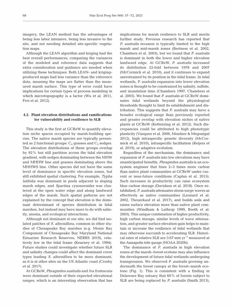
Along the tidal elevation gradient, the native gra -minoid species cluster around different elevations,with the C4 grasses dominating less frequently floo -ded areas between the MHHW and MHHWS lineswhere it floods a few times a month (Fig. 6). Schoeno-plectus americanus dominated the more frequentlyfloo ded zone between the MHHW and MHW lineswhere there are daily tides. Iva frutescens and P. aus-tralis were both much more dominant in the lowmarsh than the high marsh and had wider elevationdistribution in general. Iva frutescens had a mediangrowing elevation similar to that of S. americanus, butit had a much wider elevation distribution and domi-nated at elevations lower in the tidal range. Phrag-mites australis also occupied a relatively wide rangeof tidal elevations, occurring at both higher and lowerelevations than the native marsh vege tation andbeing more dominant in frequently flooded areas.The latter observation is based on interquartileranges of the elevation distributions, with I. fru tes censand P. australis having wider ranges in and dominance(0.100 and 0.104 m, respectively) compared to theother 2 major marsh building species (C4 = 0.100 and0.070 and S. americanus = 0.100 and 0.076 m).

Of the minor species dominant in less than 20instances, there were a few notable vertical and hor-

Mar Ecol Prog Ser 666: 57–72, 202166

Fig. 5. Performance metrics for unbiased digital elevation mapping strategies for the Global Change Research Wetland in2016 (n = 148) including the uncorrected digital elevation model (Simple Offset), the light detection and ranging (LiDAR) Ele-vation Correction with Normalized Difference Vegetation Index (LEAN), the vegetation zone corrected DEM (Veg. Class),and the kriged DEM, built independent from LiDAR. (A) Target diagram showing bias on the y-axis, unbiased root meansquare error (RMSE’) on the x-axis, and total RMSE as the sum of squares (circles). Each metric has been normalized tothe standard deviation of the reference data set so that a RMSE* value of 1 represents a performance threshold that modelsneed to be lower than to be considered efficacious. RMSE’ is artificially signed by whether the SD of the modeled (m) or

reference (r) data sets are larger. (B) RMSE* relative to ordinal values ranking strategies from most to least scalable

Holmquist et al.: Tidal elevation and wetland communities

izontal spatial trends. Spartina cynosuroides oc -curred along a wide flooding gradient and was clus-tered in a few locations, including on raised berms onthe marsh edge and on a gradual slope on themarsh’s landward edge. Typha latifolia was clusteredin continuously floo d ed depressions adjacent tosloped sections of the marsh’s landward edge.Spartina alterniflora was rare but was occasionallydominant lower in the tidal range than any other species we documented.

4. DISCUSSION

We performed an extensive survey of elevationand vegetation at the GCReW. Our comparison ofmultiple mapping strategies motivated new recom-mendations on issues of scaling in tidal wetland ele-vation mapping. The distribution of elevation acrossthe entire site, the distribution of plant species withrespect to elevation, and our field observations sug-gest several useful future studies linking the physiol-ogy and ecology of species to mechanisms of marshcollapse and expansion.

4.1. Elevation mapping techniques: tradeoffsbetween performance and scalability

Maps of elevation relative to tidal range are essen-tial tools for applying process-based models of marshresilience to SLR and identifying trends in vulnerabil-ity and resilience. However, interference of live vege-tation with LiDAR introduces elevation bias in an eco-system where plant communities are separated bycentimeters. Previous studies have developed vegeta-tion correction methods with different spatial scalesand different foci. In this study, we compared morescalable techniques, such as the single average offset,to techniques that require in crea s ing amounts of site-specific ecologic and geographic data.

One of the goals of this study was to compare mul-tiple mapping strategies for tidal marsh DEM biascorrection. All the techniques, except the constantbias correction, outperformed simply using the meanbias of the reference data, meaning that the methodswere efficacious. While the choice of correction tech-nique depends on the research questions beingasked, this study highlights limitations that resear ch -ers should consider with regard to using a constantbias correction.

For the 3 efficacious bias correction techniques,there was a general tradeoff between performanceand scalability. Spatial interpolation using kriginghad the best performance overall, followed by theLEAN-corrected DEM, and then by estimating sepa-rate corrections for different vegetation communi-ties. The LEAN-corrected DEM provided balancedtradeoffs between performance and scalability. Forinstance, Buffington et al. (2016) recommend a mini-mum of ~120 points site−1 to calibrate the statisticalmodel, provided the survey captures variation inNDVI and elevation. Freely available high-resolutionimagery from the NAIP program can be used fordeveloping the NDVI input. Because it is based on

67

Fig. 6. Probability density distribution of elevation relative tothe North American Vertical Datum of 1988 (NAVD88) at theGlobal Change Research Wetland in 2016, measured acrossthe 4 most dominant vegetation types: C4 grasses (C4), Ivafrutescens (IVFR), Phragmites australis (PHAU), and Schoe -noplectus americanus (SCAM), with the relationship to tidaldatums in 2016: MLLW: mean lower low water; MLW: meanlow water; MSL: mean sea level; MHW: mean high water;MHHW: mean higher high water; MHHWS: mean higher

high water spring; HAT: highest astronomical tide

Mar Ecol Prog Ser 666: 57–72, 2021

imagery, the LEAN method has the advantages ofbeing less labor intensive, being less invasive to thesite, and not needing detailed site-specific vegeta-tion maps.

Although the LEAN algorithm and kriging had thebest overall performances, comparing the variancesof the modeled and reference data suggests thatextra consideration and guidance are needed whenutilizing these techniques. Both LEAN- and kriging-produced maps had less variance than the referencedata, meaning the maps are flatter than the meas-ured marsh surface. This type of error could haveimplications for certain types of process modeling inwhich microtopography is a factor (Wu et al. 2011,Frei et al. 2012).

4.2. Plant elevation distributions and ramificationsfor vulnerability and resilience to SLR

This study is the first at GCReW to quantify eleva-tion niche spaces occupied by marsh-building spe-cies. The native marsh species are typically presen -ted as 2 functional groups: C4 grasses and C3 sedges.The elevation distributions of these groups overlapby 92% but still partition across the tidal elevationgradient, with sedges dominating between the MHWand MHHW line and grasses dominating above theMHHWS line. Other species did not have the samelevel of dominance in specific elevation zones, butstill exhibited spatial clustering. For example, Typhalatifolia was dominant in pools adjacent to slopingmarsh edges, and Spartina cynosuroides was clus-tered at the open water edge and along landwardedges of the marsh. Such spatial patterns are notexplained by the concept that elevation is the domi-nant determinant of species distribution in tidalmarshes, but instead may have more to do with salin-ity, anoxia, and ecological interactions.

Although not dominant at our site, we did find iso-lated patches of S. alterniflora, common in other stu -dies of Chesapeake Bay marshes (e.g. Monie BayComponent of Chesapeake Bay Maryland NationalEstuarine Research Reserves; NERRS 2019), rela-tively low in the tidal frame (Kearney et al. 1994).Future studies could investigate whether future SLRand salinity changes could affect the dominant covertypes leading S. alterniflora to be more dominant,as it is at other sites on the US Atlantic coast (Crosbyet al. 2017).

At GCReW, Phragmites australis and Iva frutescenswere dominant outside of their expected elevationalranges, which is an interesting observation that has

implications for marsh resilience to SLR and meritsfurther study. Previous research has reported thatP. australis invasion is typically limited to the highmarsh and mid-marsh zones (Bertness et al. 2002,Chambers et al. 2003), but we found that P. australisis dominant in both the lower and higher elevationlandward edge. At GCReW, P. australis increasedits distribution 22-fold between 1978 and 2007(McCormick et al. 2010), and it continues to expandunrestrained by its position in the tidal frame. In tidalwetlands, P. australis expansion into lower elevationzones is thought to be constrained by salinity, sulfide,and inundation time (Chambers 1997, Chambers etal. 2003). We found that P. australis at GCReW domi-nates tidal wetlands beyond the physiologicalthresholds thought to limit its establishment and dis-tribution. This suggests that P. australis may have abroader ecological range than previously reportedand greater overlap with elevation niches of nativeplants at GCReW (Kettenring et al. 2012). Such dis-crepancies could be attributed to high phenotypicplasticity (Vasquez et al. 2006, Mozdzer & Megonigal2012), high intraspecific genetic diversity (McCor -mick et al. 2010), intraspecific facilitation (Reijers etal. 2019), or adaptive evolution.

Regardless of the mechanism, the dominance andexpansion of P. australis into low elevations may haveunanticipated benefits. Phragmites australis is an eco-system engineer that fixes 2−3 times more carbonthan native plant communities at GCReW under cur-rent or near-future conditions (Caplan et al. 2015).Such increases in productivity can raise ecosystemblue carbon storage (Davidson et al. 2018). Once es-tablished, P. australis attenuates storm surge waves aseffectively as native communities (Leonard et al.2002, Theuerkauf et al. 2017), and builds soils andraises surface elevation more than native plant com-munities (Windham & Lathrop 1999, Rooth et al.2003). This unique combination of higher productivity,high carbon storage, similar levels of wave attenua-tion, and greater surface elevation gain helps to main-tain or increase the resilience of tidal wetlands thatmay otherwise succumb to accelerating SLR. Histori-cal rates of relative SLR are 3.67 mm yr−1 measured atthe Annapolis tide gauge (NOAA 2020b).

The dominance of P. australis in high elevationzones at the marsh−forest ecotone may also influencethe development of future tidal wetlands undergoingtransgression. We observed P. australis growing un -derneath the forest canopy at the forest−marsh eco-tone (Fig. 1). This is consistent with a finding inDelaware Bay estuary that 60% of forests subject toSLR are being replaced by P. australis (Smith 2013),

68

Holmquist et al.: Tidal elevation and wetland communities 69

and with reports of it invading newly forming tidalwetlands under ghost forests (Kirwan & Gedan2019). Future research should consider the ramifica-tions of P. australis encroachment on adjacent up -lands for efforts to conserve native plants and animalhabitat.

We found I. frutescens lower in the marsh systemthan previously reported. Iva frutescens has beencharacterized as a high marsh plant dominating thelandward edge above the S. patens zone on the USAtlantic Coast, with reduced photosynthesis even inthe absence of competitors when transplanted tothe low marsh (Bertness et al. 1992). In Louisiana,I. frutescens has been observed occupying more fre-quently flooded regions than in Rhode Island, havingoverrun S. alterniflora in created marshes (Owens etal. 2007). GCReW also shows a peak of I. frutescensdominance above MHW, but a substantial portion ofI. frutescens distribution is below the MHW line(Fig. 6). These locations tend to be adjacent to tidalcreeks, where I. frutescens either co-occurs with P.australis or Schoenoplectus americanus or has littleto no understory. Future studies should investigatewhy I. frutescens grows lower in GCReW’s tidalrange and determine if this observation is unique toGCReW. We have 3 hypotheses. First, I. frutescensmay have more phenotypic plasticity or genotypicvariation than previously recognized. Second, I. fru -tescens could truly be a high marsh plant, but sec-tions of the marsh could be collapsing due to a com-bination of SLR and muskrat herbivory destroyingthe understory plant community. The shape of theI. fru tescens elevation distribution (Fig. 6) has a peakin the high marsh between the MHHW and MHHWSlines and between the peaks of the 2 native gra -minoids, but it also has a fat tail skewing towards thelow marsh and subtidal elevation zones. We wouldexpect to see this type of a skewed distribution ifunderstory loss in some sections led to subsidencefrom loss of aerenchymous tissue and increasedorganic matter decay (Chambers et al. 2019). Third,there is growing evidence on the effects of facilita-tion and positive interactions in tidal marshes (Zhang& Shao 2013, He et al. 2013). Given that both Phrag-mites and I. frutescens are found outside their pre-dicted niches, it is possible that positive interactionsbetween these 2 species are expanding their ranges.Future studies could investigate how I. frutescensand its understory are responding to SLR and her-bivory, how soil integrity interacts with changes inplant community composition (Wigand et al. 2018),and how soil integrity relates to susceptibility to loss.To forecast marsh collapse events and the extent of

upland wetland transgressions (Kirwan & Gedan2019, Gedan & Fernández-Pascual 2019), we need todevelop a mechanistic understanding of how plantand plant−animal interactions change the distribu-tions of plant communities and the feedbacks amongbiogeochemical processes that govern elevationchange. Gathering this data will require new moni-toring and experiments across the full elevationrange of the marsh.

5. CONCLUSIONS

This study is the first extensive vegetation and ele-vation survey of the Kirkpatrick Marsh, which con-tains the GCReW, one of the most intensively studiedwetlands in the world. In the literature, the site is typ-ically discussed as a high marsh. Our study supportsthis designation because the surveyed elevation ofthe majority of marsh area fell between the MHWand MHHWS tidal datum. However, there is also asubstantial portion of the marsh that is at low eleva-tion and a skewed distribution towards zones thatflood twice daily or are constantly inundated. Weused the vegetation and elevation data we collectedto compare 4 DEM strategies. We found 3 methodswith promising results for performance and scala -bility, with the LEAN method providing a balance be-tween scalability and performance. However, thebetter-performing strategies produced maps thatwere flatter than the survey data. We observed a di-verse array of plant communities. The distributions ofthe most frequent communities were strongly partitioned along elevation gradients. The C3 sedgecommunity more frequently occupied parts of themarsh that flood daily while the C4 grass communityoccupied parts that flood a few times per month. Wedocumented a wide inundation range for the reedPhragmites australis, which may promote its successas an invasive species. Future research should furtherdocument and model interactions between floodingand plant distribution at the margins of the marsh andnear adjacent forests on the landward side of themarsh. We particularly recommend more extensivemonitoring of P. australis along the marsh−forest eco-tone and more study of elevation and soil integritywhere Iva frutescens occurs in frequently flooded areas. To conclude, this analysis adds value to paststudies at the GCReW, will help plan future experi-ments for this site or other similar sites, and providesdata on plant community distribution across elevationgradients to support cross-site synthesis and integra-tion of monitoring data and/or model results.

Mar Ecol Prog Ser 666: 57–72, 2021

Acknowledgements. Funding was primarily provided by theNASA Carbon Monitoring System (CMS; NNH14AY67I)and the Smithsonian Institution. The NSF-funded CoastalCarbon Research Coordination Network supported J.R.H.while writing this manuscript (DEB-1655622). We thankGalen Scott and Phillipe Hensel for contributing equipmentand expertise to the total station GPS surveys. We thankJames Lynch for contributing equipment and expertise tothe RTK GPS survey. We also thank Michael Hannam, BrianLamb, Sarah Freda, and Jason Swartz for their assistancewith the field work. Finally, we thank the 2 anonymousreviewers and Nichols Enwright for their constructive com-ments which improved the manuscript. Any use of trade,firm, or product names is for descriptive purposes only anddoes not imply endorsement by the US Government.

Data availability. The total station GPS, RTK GPS, and plantcover data are available via a Smithsonian FigShare DataRelease (Holmquist et al. 2021a). The vegetation maps usedto generate one of the DEMs are available via a separateSmithsonian FigShare Data release (Lu and Williams 2021).Digital Elevation Models are available via the Oak RidgeNational Labs Distributed Active Archive Center (DAAC)for Biogeochemical Dynamics (Holmquist et al. 2021b).

LITERATURE CITED

Alizad K, Hagen SC, Morris JT, Bacopoulos P, Bilskie MV,Weishampel JF, Medeiros SC (2016) A coupled, two-dimensional hydrodynamic-marsh model with biologicalfeedback. Ecol Model 327: 29−43

Alizad K, Hagen SC, Medeiros SC, Bilskie MV, Morris JT,Balthis L, Buckel CA (2018) Dynamic responses andimplications to coastal wetlands and the surroundingregions under sea level rise. PLOS ONE 13: e0205176

Alizad K, Medeiros SC, Foster-Martinez MR, Hagen SC(2020) Model sensitivity to topographic uncertainty inmeso- and microtidal marshes. IEEE J Sel Top ApplEarth Obs Remote Sens 13: 807−814

Auguie B (2017) gridextra: miscellaneous functions for ‘grid’graphics. Version 2.3. https://CRAN.R-project.org/pack-age=gridExtra

Bacopoulos P, Tritinger AS, Dix NG (2019) Sea-level riseimpact on salt marsh sustainability and migration for asubtropical estuary: GTMNERR (Guana Tolomato Ma -tanzas National Estuarine Research Reserve). EnvironModel Assess 24: 163−184

Barbier EB, Hacker SD, Kennedy C, Koch EW, Stier AC, Sil-liman BR (2011) The value of estuarine and coastal eco-system services. Ecol Monogr 81: 169−193

Bertness MD, Wikler K, Chatkupt T (1992) Flood toleranceand the distribution of Iva frutescens across New Eng-land salt marshes. Oecologia 91: 171−178

Bertness MD, Ewanchuk PJ, Silliman BR (2002) Anthro-pogenic modification of New England salt marsh land-scapes. Proc Natl Acad Sci USA 99: 1395−1398

Braun-Blanquet J (1932) Plant sociology: the study of plantcommunities. Authorized English translation of Pflan -zen soziologie. McGraw-Hill, New York, NY

Brophy LS, Greene CM, Hare VC, Holycross B and others(2019) Insights into estuary habitat loss in the westernUnited States using a new method for mapping maxi-mum extent of tidal wetlands. PLOS ONE 14: e0218558

Buffington KJ, Dugger BD, Thorne KM, Takekawa JY (2016)Statistical correction of lidar-derived digital elevationmodels with multispectral airborne imagery in tidalmarshes. Remote Sens Environ 186: 616−625

Byrd KB, Ballanti L, Thomas N, Nguyen D, Holmquist JR,Simard M, Windham-Myers L (2018) A remote sensing-based model of tidal marsh aboveground carbon stocksfor the conterminous United States. ISPRS J PhotogrammRemote Sens 139: 255−271

Cahoon DR, Lynch JC, Perez BC, Segura B and others (2002)High-precision measurements of wetland sediment ele-vation: II. The rod surface elevation table. J SedimentRes 72: 734−739

Caplan JS, Hager RN, Megonigal JP, Mozdzer TJ (2015)Global change accelerates carbon assimilation by a wet-land ecosystem engineer. Environ Res Lett 10: 115006

Castillo JM, Fernández-Baco L, Castellanos EM, Luque CJ,Figueroa ME, Davy AJ (2000) Lower limits of Spartinadensiflora and S. maritima in a Mediterranean salt marshdetermined by different ecophysiological tolerances.J Ecol 88: 801−812

Chambers RM (1997) Porewater chemistry associated withPhragmites and Spartina in a Connecticut tidal marsh.Wetlands 17: 360−367

Chambers RM, Osgood DT, Bart DJ, Montalto F (2003)Phragmites australis invasion and expansion in tidal wet-lands: interactions among salinity, sulfide, and hydrol-ogy. Estuaries 26: 398−406

Chambers LG, Steinmuller HE, Breithaupt JL (2019) Towarda mechanistic understanding of ‘peat collapse’ and itspotential contribution to coastal wetland loss. Ecology100: e02720

Chmura GL, Anisfeld SC, Cahoon DR, Lynch JC (2003)Global carbon sequestration in tidal, saline wetland soils.Global Biogeochem Cycles 17: 1111

Crosby SC, Angermeyer A, Adler JM, Bertness MD, DeeganLA, Sibinga N, Leslie HM (2017) Spartina alterniflorabiomass allocation and temperature: implications for saltmarsh persistence with sea-level rise. Estuaries Coasts40: 213−223

Davidson IC, Cott GM, Devaney JL, Simkanin C (2018) Dif-ferential effects of biological invasions on coastal bluecarbon: a global review and meta-analysis. Glob ChangeBiol 24: 5218−5230

Doughty CL, Cavanaugh KC, Hall CR, Feller IC, ChapmanSK (2017) Impacts of mangrove encroachment and mos-quito impoundment management on coastal protectionservices. Hydrobiologia 803: 105−120

Frei S, Knorr KH, Peiffer S, Fleckenstein JH (2012) Surfacemicro-topography causes hot spots of biogeochemicalactivity in wetland systems: a virtual modeling experi-ment. J Geophys Res Biogeosci 117: G00N12

Gedan KB, Fernández-Pascual E (2019) Salt marsh migra-tion into salinized agricultural fields: a novel assembly ofplant communities. J Veg Sci 30: 1007−1016

Grolemund G, Wickham H (2011) Dates and times madeeasy with lubridate. J Stat Softw 40: 1−25

He Q, Bertness MD, Altieri AH (2013) Global shifts towardspositive species interactions with increasing environ-mental stress. Ecol Lett 16: 695−706

Hladik C, Schalles J, Alber M (2013) Salt marsh elevationand habitat mapping using hyperspectral and LiDARdata. Remote Sens Environ 139: 318−330

Holmquist JR, Windham-Myers L, Bernal B, Byrd KB andothers (2018) Uncertainty in United States coastal wet-

70

Holmquist et al.: Tidal elevation and wetland communities

land greenhouse gas inventorying. Environ Res Lett 13: 115005

Holmquist J, Riera J, Shile-Beers L, Megonigal P (2021a) Elevation and vegetation data for the Global ChangeResearch Wetland, summer 2016. https://doi.org/10.25573/ serc.9589337.v1

Holmquist JR, Riera J, Megonigal JP, Shile-Beers L, Buffing -ton KJ, Weller DE (2021b) Digital elevation models forthe Global Change Research Wetland, Maryland, USA,2016. https://doi.org/10.3334/ORNLDAAC/1793

Howard J, Sutton-Grier A, Herr D, Kleypas J and others(2017) Clarifying the role of coastal and marine systemsin climate mitigation. Front Ecol Environ 15: 42−50

Janousek CN, Thorne KM, Takekawa JY (2019) Verticalzonation and niche breadth of tidal marsh plantsalong the northeast Pacific coast. Estuaries Coasts 42: 85−98

Jenkens DW (1973) Collection and analysis of remotelysensed data from the Rhode River Estuary Watershed.NASA Contractor Report 62097. https:// ntrs. nasa. gov/citations/ 19740004053

Jolliff JK, Kindle JC, Shulman I, Penta B, Friedrichs MAM,Helber R, Arnone RA (2009) Summary diagrams for cou-pled hydrodynamic-ecosystem model skill assessment.J Mar Syst 76: 64−82

Kahle D, Wickham H (2013) ggmap: spatial visualizationwith ggplot2. R J 5: 144−161

Karegar MA, Dixon TH, Engelhart SE (2016) Subsidencealong the Atlantic coast of North America: insights fromGPS and late Holocene relative sea level data. GeophysRes Lett 43: 3126−3133

Kearney MS, Stevenson JC, Ward LG (1994) Spatial andtemporal changes in marsh vertical accretion rates atMonie Bay: implications for sea-level rise. J Coast Res 10: 1010−1020

Kettenring KM, de Blois S, Hauber DP (2012) Moving froma regional to a continental perspective of Phragmitesaustralis invasion in North America. AoB Plants 2012: pls040

Kirwan ML, Gedan KB (2019) Sea-level driven land conver-sion and the formation of ghost forests. Nat Clim Chang9: 450−457

Kirwan ML, Guntenspergen GR (2015) Response of plantproductivity to experimental flooding in a stable and asubmerging marsh. Ecosystems 18: 903−913

Kirwan ML, Megonigal JP (2013) Tidal wetland stability inthe face of human impacts and sea-level rise. Nature 504: 53−60

Kirwan ML, Mudd SM (2012) Response of salt-marsh carbonaccumulation to climate change. Nature 489: 550−553

Kirwan ML, Temmerman S, Skeehan EE, GuntenspergenGR, Fagherazzi S (2016) Overestimation of marsh vulner-ability to sea level rise. Nat Clim Chang 6: 253−260

Langley JA, McKee KL, Cahoon DR, Cherry JA, MegonigalJP (2009) Elevated CO2 stimulates marsh elevation gain,counterbalancing sea-level rise. Proc Natl Acad Sci USA106: 6182−6186

Langley JA, Mozdzer TJ, Shepard KA, Hagerty SB, Megoni-gal JP (2013) Tidal marsh plant responses to elevatedCO2, nitrogen fertilization, and sea level rise. GlobChange Biol 19: 1495−1503

Leonard LA, Wren PA, Beavers RL (2002) Flow dynamicsand sedimentation in Spartina alterniflora and Phrag-mites australis marshes of the Chesapeake Bay. Wet-lands 22: 415−424

Lu M, Williams M (2021) Global Change Research Wetlandvegetation composition 1972 and 2010. https://doi.org/10. 25573/serc.12006321.v1

Lu M, Herbert ER, Langley JA, Kirwan ML, Megonigal JP(2019) Nitrogen status regulates morphological adapta-tion of marsh plants to elevated CO2. Nat Clim Chang 9: 764−768

Mader G, Schenewerk M, Weston N, Evjen J, Tadepalli K,Neti J (2012) Interactive web-based GPS network pro-cessing and adjustment using NGS’OPUS-projects. In: Proceedings of the FIg working week, Rome, 6−10 May2012. International Federation of Surveyors, Copen-hagen

McCormick MK, Kettenring KM, Baron HM, Whigham DF(2010) Extent and reproductive mechanisms of Phrag-mites australis spread in brackish wetlands in Chesa-peake Bay, Maryland (USA). Wetlands 30: 67−74

Medeiros S, Hagen S, Weishampel J, Angelo J (2015)Adjusting LiDAR-derived digital terrain models in coas -tal marshes based on estimated aboveground biomassdensity. Remote Sens 7: 3507−3525

Morris JT (2006) Competition among marsh macrophytes bymeans of geomorphological displacement in the inter-tidal zone. Estuar Coast Shelf Sci 69: 395−402

Morris JT, Bowden WB (1986) A mechanistic, numericalmodel of sedimentation, mineralization, and decomposi-tion for marsh sediments. Soil Sci Soc Am J 50: 96−105

Morris JT, Sundareshwar PV, Nietch CT, Kjerfve B, CahoonDR (2002) Responses of coastal wetlands to rising sealevel. Ecology 83: 2869−2877

Morris JT, Barber DC, Callaway JC, Chambers R and others(2016) Contributions of organic and inorganic matter tosediment volume and accretion in tidal wetlands atsteady state. Earths Future 4: 110−121

Mozdzer TJ, Megonigal JP (2012) Jack-and-master traitresponses to elevated CO2 and N: a comparison of nativeand introduced Phragmites australis. PLOS ONE 7: e42794

Mozdzer TJ, Langley JA, Mueller P, Megonigal JP (2016)Deep rooting and global change facilitate spread of inva-sive grass. Biol Invasions 18: 2619−2631

Nelson NG, Muñoz-Carpena R, Neale PJ, Tzortziou M,Megonigal JP (2017) Temporal variability in the impor-tance of hydrologic, biotic, and climatic descriptors ofdissolved oxygen dynamics in a shallow tidal-marshcreek. Water Resour Res 53: 7103−7120

NERRS (National Estuarine Research Reserve System) (2019)System-wide monitoring program. http:// nerrscdmo. org/(accessed 28 September 2018)

NOAA (2020a) Tides and currents: datums https: //tidesandcurrents.noaa.gov/datums.html?datum=MLLW&units=1&epoch=0&id=8575512&name=Annapolis&state=MD(accessed 7 August 2020)

NOAA (2020b) Tides and currents: sea level trends https: //tidesandcurrents.noaa.gov/sltrends/sltrends_station.shtml?id=8575512 (accessed 7 August 2020)

Nyman JA, Walters RJ, Delaune RD, Patrick WH (2006)Marsh vertical accretion via vegetative growth. EstuarCoast Shelf Sci 69: 370−380

Ouyang X, Lee SY (2013) Carbon accumulation rates in saltmarsh sediments suggest high carbon storage capacity.Biogeosciences Discuss 10: 19155−19188

Owens AB, Proffitt CE, Grace JB (2007) Prescribed fire andcutting as tools for reducing woody plant succession in acreated salt marsh. Wetlands Ecol Manage 15: 405−416

71

Mar Ecol Prog Ser 666: 57–72, 202172

Park RA, Trehan MS, Mausel PW, Howe RC (1989) Theeffects of sea level rise on US coastal wetlands. In: SmithJB, Tirpak DA (eds) The potential effects of global cli-mate change on the United States: Appendix B — sealevel rise. US Environmental Protection Agency, Wash-ington, DC, p 1−55

R Core Team (2019) R: a language and environment for statistical computing. R Foundation for Statistical Com-puting, Vienna

Reijers VC, Akker M, Cruijsen PMJM, Lamers LPM, HeideT (2019) Intraspecific facilitation explains the persistenceof Phragmites australis in modified coastal wetlands.Ecosphere 10: 633

Rice D, Rooth J, Stevenson JC (2000) Colonization andexpansion of Phragmites australis in upper ChesapeakeBay tidal marshes. Wetlands 20: 280

Rooth JE, Stevenson JC, Cornwell JC (2003) Increased sed-iment accretion rates following invasion by Phragmitesaustralis: the role of litter. Estuaries 26: 475−483

Saltonstall K (2002) Cryptic invasion by a non-native geno-type of the common reed, Phragmites australis, intoNorth America. Proc Natl Acad Sci USA 99: 2445−2449

Schile LM, Callaway JC, Morris JT, Stralberg D, Parker VT,Kelly M (2014) Modeling tidal marsh distribution with sea-level rise: evaluating the role of vegetation, sediment, andupland habitat in marsh resiliency. PLOS ONE 9: e88760

Smith JAM (2013) The role of Phragmites australis in medi-ating inland salt marsh migration in a Mid-Atlantic estu-ary. PLOS ONE 8: e65091

Snedden GA, Steyer GD (2013) Predictive occurrence mod-els for coastal wetland plant communities: delineatinghydrologic response surfaces with multinomial logisticregression. Estuar Coast Shelf Sci 118: 11−23

Stephenson AG (2016) Harmonic analysis of tides usingtideharmonics. Version 0.1-1. https://cran.r-project. org/web/ packages/ Tide Harmonics/ index.html

Swanson KM, Drexler JZ, Schoellhamer DH, Thorne KMand others (2014) Wetland accretion rate model of eco-system resilience (WARMER) and its application to habi-tat sustainability for endangered species in the San Fran-cisco Estuary. Estuaries Coasts 37: 476−492

Theuerkauf SJ, Puckett BJ, Theuerkauf KW, Theuerkauf EJ,Eggleston DB (2017) Density-dependent role of an inva-sive marsh grass, Phragmites australis, on ecosystemservice provision. PLOS ONE 12: e0173007

Thorne K, Buffington K, Swanson K, Takekawa J (2013)Storm surges and climate change implications for tidalmarshes: insight from the San Francisco Bay Estuary,California, USA. Int J Clim Chang Impacts Resp 4: 169−190

Thorne K, MacDonald G, Guntenspergen G, Ambrose R andothers (2018) US Pacific coastal wetland resilience andvulnerability to sea-level rise. Sci Adv 4: eaao3270

US Fish and Wildlife Service (2014) National WetlandsInventory. https: //www.fws.gov/wetlands/

Vasquez EA, Glenn EP, Guntenspergen GR, Brown JJ, Nel-son SG (2006) Salt tolerance and osmotic adjustment ofSpartina alterniflora (Poaceae) and the invasive M hap-lotype of Phragmites australis (Poaceae) along a salinitygradient. Am J Bot 93: 1784−1790

Wickham H (2016) ggplot2: elegant graphics for data ana -lysis. Version 3.3.3. https://ggplot2.tidyverse.org

Wickham H, François R, Henry L, Müller K (2019) dplyr: agrammar of data manipulation. Version 0.8.3. https://CRAN. R-project. org/ package = dplyr

Wigand C, Watson EB, Martin R, Johnson DS and others(2018) Discontinuities in soil strength contribute to desta-bilization of nutrient-enriched creeks. Ecosphere 9: e02329

Windham L, Lathrop RG (1999) Effects of Phragmites aus-tralis (common reed) invasion on aboveground biomassand soil properties in brackish tidal marsh of the MullicaRiver, New Jersey. Estuaries 22: 927−935

Wu J, Roulet NT, Moore TR, Lafleur P, Humphreys E (2011)Dealing with microtopography of an ombrotrophic bogfor simulating ecosystem-level CO2 exchanges. EcolModel 222: 1038−1047

Zeileis A, Grothendieck G (2005) zoo: S3 infrastructure forregular and irregular time series. J Stat Softw 14: 1−27

Zhang L, Shao H (2013) Direct plant−plant facilitation incoastal wetlands: a review. Estuar Coast Shelf Sci 119: 1−6

Editorial responsibility: Jana Davis, Annapolis, Maryland, USA

Reviewed by: 2 anonymous referees

Submitted: April 14, 2020Accepted: March 1, 2021Proofs received from author(s): May 4, 2021